Prescribed Robustness in Optimal Power Flow

Abstract

For a timely decarbonization of our economy, power systems need to accommodate increasing numbers of clean but stochastic resources. This requires new operational methods that internalize this stochasticity to ensure safety and efficiency. This paper proposes a novel approach to compute adaptive safety intervals for each stochastic resource that internalize power flow physics and optimize the expected cost of system operations, making them “prescriptive”. The resulting intervals are interpretable and can be used in a tractable robust optimal power flow problem as uncertainty sets. We use stochastic gradient descent with differentiable optimization layers to compute a mapping that obtains these intervals from a given vector of context parameters that captures the expected system state. We demonstrate and discuss the proposed approach on two case studies.

I Introduction

The ongoing deployment of clean but stochastic energy resources challenges established power system operations by threatening their ability to ensure system security and economic efficiency. To tackle this, numerous effective stochastic optimizations methods have been proposed, covering, for example, system scheduling and control [1, 2, 3] or electricity markets and the unit commitment process [4, 5], and inertia provision [6, 7]. However, the adoption of [1, 2, 3, 4, 5, 6, 7] and similar proposals is obstructed by the necessity to significantly alter established operations, an expensive and risky process for system operators. Moreover, stochastic approaches to power system operations typically optimize reserve allocations and control policies implicitly based on probabilistic models and risk parameters defined by the system operator. This complicates a transparent communication towards power system stakeholders (e.g., owners of generation assets, electricity market participants who are interested in anticipating price formation and scheduling procedures). To overcome these barriers and further facilitate the adoption of clean energy technology, actionable methods for power system operation and planning that smartly internalize resource stochasticity while remaining interpretable and largely compatible with established processes are required.

Motivated by this requirement, this paper proposes a data-driven approach inspired by [8] to compute uncertainty sets for stochastic resources that (i) robustify generation and reserve allocation, (ii) internalize system physics, and (iii) minimize risk-adjusted cost while avoiding the need for a stochastic decision-making process. Deviating from [8], we introduce an additional prescription step that allows to adjust the uncertainty sets based on the problem context.

I-A General problem formulation

Consider power system operations as a two-stage optimization problem with uncertain parameters $\bm{\xi}$, e.g., real-time nodal demand or renewable energy injection. Given a current parametrization of the system $\bm{\zeta}$ (e.g., net-demand forecast, generator availability), the first stage computes a resource allocation $\bm{x}$ (e.g., generation schedules, reserve allocations). The second stage then decides on recourse actions $\bm{y}$ depending on the first-stage allocation $\bm{x}^{*}$ and the realization of $\bm{\xi}$. In current industry practice, the two stages are solved deterministically and independently using fixed security parameters $\bm{\theta}$ (e.g., reserve requirements) in the first stage:

$$\text{1st stage:}\quad\hskip 18.00005pt\mathcal{P}(\bm{\zeta},\bm{\theta}) =\min_{\bm{x}\in\mathscr{X}(\bm{\zeta},\bm{\theta})}\mathcal{C}^{\rm F}(\bm{x},\bm{\zeta},\bm{\theta})$$ (1)

$$\text{2nd stage:}\quad\mathcal{Q}(\bm{x}^{*},\bm{\zeta},\bm{\xi}) =\min_{\bm{y}\in\mathscr{Y}(\bm{x}^{*},\bm{\zeta},\bm{\xi})}\mathcal{C}^{\rm S}(\bm{x}^{*},\bm{\zeta},\bm{\xi})$$ (2)

While this process is computationally efficient and transparent, it ignores any probabilistic information that my be available from models or historic observations of $\bm{\xi}$.

As an alternative to replacing this deterministic two-step procedure with probabilistic optimization (see discussion above), this paper proposes an adaptive computation of parameters $\bm{\theta}$ that internalizes information on the stochasticity of $\bm{\xi}$ and is aware of $\bm{\zeta}$. We highlight that vector $\bm{\zeta}$ can be considered richer than just containing problem parameters, but may also contain additional covariates of $\bm{\xi}$ (e.g., weather information, forecasts). We therefore call $\bm{\zeta}$ context parameters. Given $\bm{\zeta}$, the optimal choice of $\bm{\theta}$ in the first stage is

$$\bm{\theta}^{*}(\bm{\zeta})\in\operatorname*{arg\,min}_{\bm{\theta}}\mathbb{E}_{(\bm{\xi}\mid\bm{\zeta})}\big{[}\mathcal{P}(\bm{\zeta},\bm{\theta})+\mathcal{Q}(\bm{x}^{*},\bm{\zeta},\bm{\xi})\big{]},$$ (3)

Following [9], we call $\bm{\theta}^{*}$ prescriptive in the context of $\bm{\zeta}$, as it provides a parametrization that minimizes the conditional expectation over $\bm{\xi}$. To avoid re-solving 3 every time (which might be hard or impossible), the objective of this paper is to obtain a mapping $\mathcal{M}$ that computes $\bm{\theta}^{*}$ from $\bm{\zeta}$, i.e.:

$$\min_{\mathcal{M}}\mathbb{E}_{(\bm{\zeta,\bm{\xi}})}\big{[}\mathcal{P}(\bm{\zeta},\mathcal{M}(\bm{\zeta}))+\mathcal{Q}(\bm{x^{*}},\bm{\zeta},\bm{\xi})].$$ (4)

Solving problem 4 is hard in general and its tractability depends on the definition of the operational problem $\mathcal{P}$, $\mathcal{Q}$ and the mapping $\mathcal{M}$. This paper studies the following approach:

• For $\mathcal{P}$ and $\mathcal{Q}$ we focus on an optimal power flow (OPF) problem where the first stage computes a reserve allocation and a second-stage control policy that ensures system safety for predefined uncertainty regions given by $\bm{\theta}$. This approach follows the idea of robust optimization, but we can avoid overly conservative solutions by properly tuning $\bm{\theta}$. Section II explains the model in detail.

• For $\mathcal{M}$ we focus on an interpretable linear model $\mathcal{M}_{\bm{w}}(\bm{\zeta})=\bm{M}\bm{\zeta}+\bm{m}$ parametrized by $\bm{w}=(\bm{M},\bm{m})$ similar to the approach in [10]. We will refer to $\bm{w}$ as weights throughout this paper to avoid confusion with parameters $\bm{\zeta}$ and $\bm{\theta}$.

• The resulting problem is a bi-level program that we solve using stochastic gradient descent with differentiable optimization layers. We discuss this in Section III.

I-B Related literature

Robust optimization for OPF has been studied alongside numerous proposals for general stochastic OPF. Mainly introduced by the seminal work in [5], robust OPF can provide security with manageable computational complexity and transparent communication of the considered uncertain region for each resource. More recent variants include data-driven approaches [11] and tractable extensions to AC-OPF [12, 2]. However, how to define good uncertainty sets that avoid overly conservative results remains tricky [13].

Adoption barriers for stochastic optimization in power systems have been previously highlighted in [14, 15] and options for approximating their performance with no or little alteration of current industry practice have been explored in [16, 14, 15, 17, 10]. While [16, 15] study more flexible reserve products and reserve requirements informed by an auxiliary stochastic program, respectively, [14, 17, 10] propose methods that prescribe intentionally biased input parameters (forecasts) to the first stage problem. This approach fits our formulations in 3 and 4. In [14] the authors solve a bi-level program for each instance of the first stage to obtain a (prescriptive) alternative wind power forecast. Building on this idea, [10] computes a mapping from the original to a prescribed net-demand forecast. To this end, the authors include the first stage optimality conditions in the second stage to compute the map using in a single stochastic program. Pursuing the similar objective of obtaining optimally biased forecasts that reflect the asymmetric power system cost structure (generation excess can typically be handled more cheaply than shortage), [17] propose a bi-level program with a scaleable solution heuristic.

Models (e.g., for forecasting) that minimize the loss of a downstream optimization task have gained general popularity as end-to-end learning [18] or smart predict-and-optimize [19]. Many exciting results in this direction have been unlocked by differentiable optimization frameworks, e.g., [20], that enable efficient iterative model training procedures that internalize optimization layers. For example, [21] train a demand forecast model that minimizes the expected cost of generation excess and shortage, [7] train a generative network to obtain adversarial forecast scenarios to improve reserve allocation, [22] create a wind power forecast model that minimizes wind spillage, and [23] tune their wind power prediction model to minimize forecast errors in resulting electricity prices.

II Operation model

We consider a short-term generator dispatch problem with balancing control (e.g., automatic generator control) with uncertain injections from stochastic wind generators. We model these uncertain injections as a $D$-dimensional vector $\bm{u}(\bm{\xi})=\bm{u}+\bm{\xi}$, where $\bm{u}$ is a (deterministic) forecast and $\bm{\xi}$ is a vector of random forecast errors. Power imbalance caused by forecast errors $\bm{\xi}$ are corrected by controllable generators. The generator output is a $G$-dimensional vector $\bm{p}(\bm{\xi})=\bm{p}-\bm{A}\bm{\xi}$. By ensuring $\bm{A}^{\mkern-1.0mu\mathsf{T}}\bm{1}_{G}=\bm{1}_{D}$, where $\bm{1}_{D}$ is a $D$-dimensional vector of ones, all forecast errors are balanced.

II-A Robust optimal power flow with fixed recourse

To immunize the system against uncertain injections $\bm{u}(\bm{\xi})$, $\bm{p}(\bm{\xi})$ and the resulting uncertain power flows, the system operator defines an uncertainty set $\mathscr{U}$ that captures all outcomes of $\bm{\xi}$ for which all system constrains should hold. Given a parametrization $\bm{\zeta}$ (forecast $\bm{u}$ and demand vector $\bm{d}$) the system operator then solves the following robust OPF problem to decide on the generator dispatch $\bm{p}$ and reserves $\bm{r^{+}}$, $\bm{r^{-}}$:

$$\min\quad (\bm{c}^{\rm E})^{\mkern-1.0mu\mathsf{T}}\bm{p}+(\bm{c}^{\rm R})^{\mkern-1.0mu\mathsf{T}}(\bm{r}^{+}+\bm{r}^{-})$$ (5a)

s.t. $$\bm{1}_{G}^{\mkern-1.0mu\mathsf{T}}\bm{p}=\bm{1}_{V}^{\mkern-1.0mu\mathsf{T}}\bm{d}-\bm{1}_{D}^{\mkern-1.0mu\mathsf{T}}\bm{u}$$ (5b)

$$\bm{A}^{\mkern-1.0mu\mathsf{T}}\bm{1}_{G}=\bm{1}_{D}$$ (5c)

$$\bm{p}+\bm{r}^{+}\leq\bm{p}^{\rm max}$$ (5d)

$$\bm{p}-\bm{r}^{-}\geq\bm{p}^{\rm min}$$ (5e)

$$\bm{B}^{\rm G}\bm{p}+\bm{B}^{\rm W}\bm{u}-\bm{B}^{\rm B}\bm{d}=\bm{f}^{\rm max}-\bm{f}^{\rm RAM+}$$ (5f)

$$-(\bm{B}^{\rm G}\bm{p}+\bm{B}^{\rm W}\bm{u}-\bm{B}^{\rm B}\bm{d})=\bm{f}^{\rm max}-\bm{f}^{\rm RAM-}$$ (5g)

$$-\bm{A}\bm{\xi}\leq\bm{r}^{+} \forall\bm{\xi}\in\mathscr{U}$$ (5h)

$$\bm{A}\bm{\xi}\leq\bm{r}^{-} \forall\bm{\xi}\in\mathscr{U}$$ (5i)

$$(\bm{B}^{\rm W}-\bm{B}^{\rm G}\bm{A})\bm{\xi}\leq\bm{f}^{\rm RAM+}\! \forall\bm{\xi}\in\mathscr{U}$$ (5j)

$$-(\bm{B}^{\rm W}-\bm{B}^{\rm G}\bm{A})\bm{\xi}\leq\bm{f}^{\rm RAM-}\! \forall\bm{\xi}\in\mathscr{U}$$ (5k)

The objective 5a minimizes system cost given energy cost and reserve provision cost vectors $\bm{c}^{\rm E}$ and $\bm{c}^{\rm R}$. Energy balance 5b ensures that the total generator injections equals the total system demand $\bm{d}$ and $\bm{u}$. Similarly, 5c ensures that all forecast errors are balanced. Constraints 5d and 5e enforce the technical production limits of each controllable generator. Constraints 5f and 5g map the power injections and withdrawals of each resource and load to a resulting power flow using suitable linear maps [24], e.g., obtained from the DC power flow approximation. Vectors $\bm{f}^{\rm RAM+}$ and $\bm{f}^{\rm RAM-}$ are the remaining available margins for each power transmission line, i.e., the difference between the power flow caused by the forecast injections and the upper and lower line limits. Constraints 5i, 5h, 5k and 5j enforce robust constraints on the system response to uncertain forecast errors $\bm{\xi}$. Constraints 5i and 5h ensure that generator balancing responses do not exceed the available reserves and 5k and 5j ensure that the resulting power flow changes do not exceed the remaining available margins on each power line for any $\bm{\xi}\in\mathscr{U}$.

Problem 5 can be re-written in a more concise form. We collect all decision variables in a vector $\bm{x}$, cost vectors $\bm{c}^{\rm E}$, $\bm{c}^{\rm R}$ in a vector $\bm{c}$, denote the feasible space defined by constraints 5c, 5b, 5d, 5e, 5f and 5g as $\mathscr{F}(\bm{\zeta})$ and write:

$$\min_{\bm{x}\in\mathscr{F}(\bm{\zeta})}\ \bm{c}^{\mkern-1.0mu\mathsf{T}}\bm{x}$$ (6a)

s.t. $$\max_{k=1,...,K}[\bm{a}_{k}^{\mkern-1.0mu\mathsf{T}}\bm{\xi}+b_{k}]\leq 0,\quad\forall\bm{\xi}\in\mathscr{U}$$ (6b)

where $\bm{a}_{k}$ and $b_{k}$ are, respectively, the $k$-th row and $k$-th entry of the $K\times D$ matrix and $K\times 1$ vector

$$\begin{bmatrix}-\bm{A}\\ \bm{A}\\ (\bm{B}^{\rm\bm{W}}-\bm{B}^{\rm G}\bm{A})\\ -(\bm{B}^{\rm W}-\bm{B}^{\rm G}\bm{A})\end{bmatrix}\text{ and }\begin{bmatrix}-\bm{r}^{+}\\ -\bm{r}^{-}\\ -\bm{f}^{\rm RAM+}\\ -\bm{f}^{\rm RAM-}\end{bmatrix}.$$

Note that 6b is an exact reformulation of 5i, 5h, 5k and 5j as the maximum of $K$ affine functions.

II-B Uncertainty set formulation

Model 5 cannot be solved directly but requires a definition of $\mathscr{U}$ alongside a tractable reformulation of constraints 5i, 5h, 5k and 5j. This paper focuses on box uncertainty sets, as they provide a clear safety region for each uncertain resource. Other formulations are possible [25]. Box uncertainty sets ensure that constraints are feasible for a security interval along each dimension of the uncertain vector $\bm{\xi}$. We can define such a set as $\mathscr{U}^{\rm box}(\bm{\theta})=\{\xi_{j}|\xi_{j}\in[\mu_{j}-\sigma_{j},\mu_{j}+\sigma_{j}],\ j=1,...,D\}$ parametrized by $\bm{\theta}=(\bm{\mu},\bm{\sigma})$ with $\bm{\mu}=[\mu_{1},...,\mu_{D}]$ and $\bm{\sigma}=[\sigma_{1},...,\sigma_{D}]$. Parameter $\bm{\mu}$ is the center of the security interval and can be interpreted as a forecast error bias. Parameter $\bm{\sigma}$ defines the width of the interval. Using $\mathscr{U}=\mathscr{U}^{\rm box}$ and introducing auxiliary variable $\bm{t}_{k}$, 6b becomes

$$\bm{a}_{k}^{\mkern-1.0mu\mathsf{T}}\bm{\mu}+\bm{t}_{k}^{\mkern-1.0mu\mathsf{T}}\bm{\sigma}\leq b_{k},\ \bm{t}_{k}\geq|\bm{a}_{k}|,\quad\forall k=1,..,K.$$ (7)

See also [26] for an in-depth discussion on robust counterparts of constraints with the form of 6b.

II-C Real-time cost and security

The choice of uncertainty set parameters $\bm{\theta}$ implies a trade-off between security in real-time and cost in the first-stage decision. For example, choosing $\bm{\theta}$ such that $\mathscr{U}$ is large and covers all potential outcomes of $\bm{\xi}$ will lead to high security in real-time but also to high first-stage cost. A good choice of $\bm{\theta}$ will balance this trade-off by minimizing the combined first- and second-stage cost as defined in 3. We consider two relevant approaches to quantify security of the robust problem from Section II-A in real-time.

II-C1 Cost of exceedance

We can define the real-time cost as cost of exceedance by imposing a penalty for insufficient reserves $\bm{r}^{+}$, $\bm{r}^{-}$, $\bm{f}^{\rm RAM+}$, $\bm{f}^{\rm RAM-}$. Using the notation from 6, we compute this cost as

$$\mathcal{C}^{\rm S}(\bm{x},\bm{\xi})=\sum_{k=1}^{K}c_{k}^{\rm viol}\big{[}\bm{a}_{k}^{\mkern-1.0mu\mathsf{T}}\bm{\xi}+b_{k}\big{]}^{+},$$ (8)

where $[\cdot]^{+}=\max\{\cdot,0\}$ and $c_{k}^{\rm viol}$ is the cost for exceeding the reserve given by $b_{k}$. Cost $c_{k}^{\rm viol}$ could, for example, reflect the cost of procuring emergency resources or load shedding.

II-C2 Probability of exceedance

Instead of minimizing cost of exceedance, the system operator may be interested in a probabilistic guarantee that real-time operations do not exceed reserves, i.e.:

$$\mathbb{P}\Big{[}\max_{k=1,...,K}[\bm{a}_{k}^{\mkern-1.0mu\mathsf{T}}\bm{\xi}+b_{k}]<0\Big{]}\geq 1-\gamma.$$ (9)

Here, $(1-\gamma)$ defines the target probability of no constraint exceeding its limits and $\gamma$ is a small risk factor.

III Solution Approach

We now show an iterative method inspired by the results in [8] to obtain the desired mapping $\mathcal{M}_{\bm{w}}(\bm{\zeta})=\bm{M}\bm{\zeta}+\bm{m}$ that returns uncertainty set parameters $\bm{\theta}$, which, in turn, optimally parametrize the first-stage uncertainty set with respect to the cost and probability of exceedance discussed in Section II-C.

III-A Cost of exceedance

The problem to compute the optimal choice of weights $\bm{w}=(\bm{M},\bm{m})$ that minimize the combined expected first- and second-stage cost is the bi-level problem:

$$\min_{\bm{w}}\quad \mathbb{E}_{(\bm{\zeta},\bm{\xi})}\big{[}\bm{c}^{\mkern-1.0mu\mathsf{T}}\bm{x}^{*}+\mathcal{C}^{\rm S}(\bm{x}^{*},\bm{\xi})\big{]}$$ (10a)

s.t. $$\bm{\theta}=\mathcal{M}_{\bm{w}}(\bm{\zeta})$$ (10b)

$$\bm{x}^{*}(\bm{\zeta},\bm{\theta})\!\in\!\left\{\begin{array}[]{l}\!\!\operatorname*{arg\,min}_{\bm{x}\in\mathscr{F}(\bm{\zeta})}\ \!\bm{c}^{\mkern-1.0mu\mathsf{T}}\bm{x}\\[5.59721pt] \!\!\text{s.t.}\ \max_{k}[\bm{a}_{k}^{\mkern-1.0mu\mathsf{T}}\bm{\xi}+b_{k}]\!\leq\!0,\ \forall\bm{\xi}\!\in\!\mathscr{U}(\bm{\theta}).\end{array}\right.$$ (10e)

We solve 10 using a stochastic gradient descent approach with $v^{\rm max}$ outer steps (epochs) indexed by $v$ and $z^{\rm max}$ inner steps (“mini-batches” [27]) indexed by $z$. For each step $z$ we assume to have access to an individual context parameter sample $\bm{\zeta}^{z}$ (e.g., obtained from historic observations or a sample generation mechanism) and a set of $N_{z}$ samples $\mathscr{X}^{z}=\{\bm{\xi}_{i}^{z}\}_{i=1}^{N_{z}}$ of $\bm{\xi}$ (again, either obtained from historical observations or a sample generation mechanism). We note that $\mathscr{X}^{z}$ may be conditional to $\bm{\zeta}^{z}$. See, for example, [28] who also provide an approach to sample $\mathscr{X}^{z}$ for a given wind power forecast $\bm{u}^{z}$ (which is part of the parametrization $\bm{\zeta}^{z}$). We provide additional discussion on the relationship between $\bm{\zeta}^{z}$ and $\mathscr{X}^{z}$ in the case study below. We define $\bm{x}^{z}=\bm{x}^{*}(\bm{\zeta}^{z},\bm{\theta}^{z})$ as the solution to the inner problem 10e. The loss function $L(\bm{w}^{z};\bm{\zeta}^{z},\bm{\xi}^{z})$ corresponds to the problem objective in 10e and we compute it as the empirical mean given $\mathscr{X}^{z}$:

$$L^{\rm C}\!(\bm{w}^{z}\!;\bm{\zeta}^{z}\!,\mathscr{X}^{z}\!)\!=\!\bm{c}^{\mkern-1.0mu\mathsf{T}}\bm{x}^{z}\!+\!\frac{1}{N_{z}}\!\sum_{i=1}^{N_{z}}\sum_{k=1}^{K}\!c_{k}\big{[}(\bm{a}_{k}^{z})^{\mkern-1.0mu\mathsf{T}}\bm{\xi}_{i}^{z}\!+\!b_{k}^{z}\big{]}^{+}.$$ (11)

Recall from 6b that $\bm{a}_{k}$ and $b_{k}$ are decision variables and a part of $\bm{x}$. Following [8] we estimate the derivative of $L(\bm{w}^{z};\bm{\zeta}^{z},\bm{\xi}^{z})$ using a subgradient $G^{\rm C}(\bm{w}^{z};\bm{\zeta}^{z},\mathscr{X}^{z})$ computed over samples of $\bm{\zeta}$ and $\bm{\xi}$. Notably, the computation of $G^{\rm C}(\bm{w}^{z};\bm{\zeta}^{z},\mathscr{X}^{z})$ requires computing gradient $\nabla_{\bm{\theta}}\bm{x}^{*}(\bm{\zeta},\bm{\theta})$, i.e., the derivative of the decision variables of the inner problem over the uncertainty set parameters. We discuss an efficient approach to obtain this gradient in Section III-C below. Choosing initial weights $(\bm{M}^{\rm init},\bm{m}^{\rm init})$ and a learning rate $\rho$ the resulting solution steps are itemized in Algorithm 1.

Algorithm 1 Stochastic gradient descent to solve 10

1:given $\bm{w}^{0}=(\bm{M}^{\rm init},\bm{m}^{\rm init})$, learning rate $\rho$

2:for $v=1,...,v^{\rm max}$ do $\triangleright$ outer epoch

3:     for $z=1,...,z^{\rm max}$ do $\triangleright$ inner mini-batch

4:         $\bm{\zeta}^{z}\leftarrow$ sample context parameter

5:         $\mathscr{X}^{z}\leftarrow$ sample forecast errors conditional to $\bm{\zeta}^{z}$

6:         $\bm{\theta}^{z}\leftarrow\mathcal{M}_{\bm{w}^{v-1}}(\bm{\zeta}^{z})$ $\triangleright$ prescribe parameters

7:         $\bm{x}^{z}\leftarrow$ solve inner problem 10e

8:         $\bm{g}^{z}\leftarrow G^{\rm C}(\bm{w}^{v-1};\bm{\zeta}^{z},\mathscr{X}^{z})$      

9:     $\bm{g}^{v}\leftarrow\frac{1}{z^{\rm max}}\sum_{z=1}^{z^{\rm max}}\bm{g}^{z}$ $\triangleright$ update gradient

10:     $\bm{w}^{v}\leftarrow\bm{w}^{v-1}\!-\!\rho\bm{g}^{v}$ $\triangleright$ update variables

11:return $\bm{w}^{v^{\rm max}}$

III-B Probability of exceedance

The problem to compute the optimal choice of weights $\bm{w}$ that ensure real-time operations do not exceed their limits with a probability of at least $(1-\gamma)$ is the bi-level problem:

$$\min_{\bm{w}}\quad \mathbb{E}_{(\bm{\zeta},\bm{\xi})}\big{[}\bm{c}^{\mkern-1.0mu\mathsf{T}}\bm{x}^{*}\big{]}$$ (12a)

s.t. $$\mathbb{P}\Big{[}\max_{k=1,...,K}[(\bm{a}_{k}^{*})^{\mkern-1.0mu\mathsf{T}}\bm{\xi}+b_{k}^{*}]<0\Big{]}\geq 1-\gamma$$ (12b)

$$\big{[}\text{$\bm{\theta}$ and $\bm{x}^{*}(\bm{\zeta,\bm{\theta}})$ as in \lx@cref{creftypeplural~refnum}{eq:coe_prescription} and~\lx@cref{refnum}{eq:coe_inner}}\big{]}.$$ (12c)

Constraint 12b is generally non-convex and complicates the solution of 12. To create a tractable problem, we reformulate 12b using conditional value-at-risk [8, 29]:

$$\mathbb{P}\big{[}\max_{k=1,...,K}[\bm{a}_{k}^{\mkern-1.0mu\mathsf{T}}\bm{\xi}+b_{k}\leq 0\big{]}\geq 1-\gamma$$ (13)

$$\Leftrightarrow \operatorname{VaR}_{\gamma}\big{(}\max_{k=1,...,K}[\bm{a}_{k}^{\mkern-1.0mu\mathsf{T}}\bm{\xi}+b_{k}]\big{)}\leq 0$$

$$\Leftarrow \operatorname{CVaR}_{\gamma}\big{(}\max_{k=1,...,K}[\bm{a}_{k}^{\mkern-1.0mu\mathsf{T}}\bm{\xi}+b_{k}]\big{)}\leq 0$$

where $\operatorname{VaR}_{\gamma}$ and $\operatorname{CVaR}_{\gamma}$ are the value-at-risk and conditional value-at-risk at risk level $\gamma$. Reformulation 13 utilizes the fact that limiting CVaR implies a limit on VaR [30]. CVaR further allows the convex reformulation [30]

$$\operatorname{CVaR}_{\gamma}=\inf_{\tau}\Big{\{}\mathbb{E}\Big{[}\frac{1}{\gamma}\big{[}\max_{k=1,...,K}[\bm{a}_{k}^{\mkern-1.0mu\mathsf{T}}\bm{\xi}+b_{k}]-\tau\big{]}^{+}+\tau\Big{]}\Big{\}},$$ (14)

which we use to define

$$h(\bm{x}^{*},\tau,\bm{\xi})=\frac{1}{\gamma}\big{[}\max_{k=1,...,K}[\bm{a}_{k}^{\mkern-1.0mu\mathsf{T}}\bm{\xi}+b_{k}]-\tau\big{]}^{+}+\tau,$$ (15)

and to reformulate 12 as [8]:

$$\min_{\bm{w},\tau}\quad \mathbb{E}_{(\bm{\zeta},\bm{\xi})}\big{[}\bm{c}^{\mkern-1.0mu\mathsf{T}}\bm{x}^{*}\big{]}$$ (16a)

s.t. $$\mathbb{E}_{(\bm{\zeta},\bm{\xi})}\big{[}h(\bm{x}^{*},\tau,\bm{\xi})\big{]}=0$$ (16b)

$$\big{[}\text{$\bm{\theta}$ and $\bm{x}^{*}(\bm{\zeta,\bm{\theta}})$ as in \lx@cref{creftypeplural~refnum}{eq:coe_prescription} and~\lx@cref{refnum}{eq:coe_inner}}\big{]}.$$ (16c)

We note that 16 has an additional auxiliary variable $\tau$ related to the CVaR reformulation 14. Also, following the logic in [8], we note that 16b is an equality constraint, because zero is the optimal CVaR target given 13 and the convexity of 14.

Similar to he procedure outlined in [8, 31] we can now solve the equality-constrained problem 16 by introducing Lagrangian multiplier $\lambda$ and defining the loss function

$$L^{\rm P}((\bm{w}\!,\tau);\lambda\!,\bm{\zeta}\!,\bm{\xi})\!=\!\mathbb{E}_{(\bm{\zeta},\bm{\xi})}\big{[}\bm{c}^{\mkern-1.0mu\mathsf{T}}\bm{x}^{*}\big{]}\!+\!\lambda\mathbb{E}_{(\bm{\zeta},\bm{\xi})}\big{[}h(\bm{x}^{*}\!,\tau\!,\bm{\xi})\big{]}.$$ (17)

Using the notation introduced in Section III-A above, we compute 17 in each step $z$ as

$$L^{\rm P}((\bm{w}^{z},\tau^{z});\lambda^{z},\bm{\zeta}^{z},\mathscr{X}^{z})=$$ (18)

$$\quad\bm{c}^{\mkern-1.0mu\mathsf{T}}\bm{x}^{z}\!+\!\lambda^{z}\underbrace{\frac{1}{N_{z}}\sum_{i=1}^{N_{z}}\!\!\Big{(}\frac{1}{\gamma}\big{[}\max_{k=1,...,K}[(\bm{a}_{k}^{z})^{\mkern-1.0mu\mathsf{T}}\bm{\xi}_{i}^{z}\!+\!b_{k}^{z}]\!-\!\tau^{z}\big{]}^{+}\!\!+\!\tau^{z}\Big{)}}_{H((\bm{w}^{z},\tau^{z});\bm{\zeta}^{z},\mathscr{X}^{z})}.$$

Denoting $G^{\rm P}((\bm{w}^{z},\tau^{z});\lambda^{z},\bm{\zeta}^{z},\mathscr{X}^{z})$ as the gradient of 18, $\tau^{\rm init}$, $\lambda^{\rm init}$ as initial values for $\tau$, $\lambda$, and $\kappa$ as the step size for $\lambda$ the resulting solution steps are itemized in Algorithm 2.

Algorithm 2 Stochastic gradient descent to solve 12

1:given $\bm{w}^{0}=(\bm{M}^{\rm init},\bm{m}^{\rm init})$, $\tau^{0}=\tau^{\rm init}$, $\lambda^{0}=\lambda^{\rm init}$, $\rho$, $\kappa$

2:for $v=1,...,v^{\rm max}$ do $\triangleright$ outer epoch

3:     for $z=1,...,z^{\rm max}$ do $\triangleright$ inner mini-batch

4:         $\bm{\zeta}^{z}\leftarrow$ sample context parameter

5:         $\mathscr{X}^{z}\leftarrow$ sample forecast errors conditional to $\bm{\zeta}^{z}$

6:         $\bm{\theta}^{z}\leftarrow\mathcal{M}_{\bm{w}^{v-1}}(\bm{\zeta}^{z})$ $\triangleright$ prescribe parameters

7:         $\bm{x}^{z}\leftarrow$ solve inner problem 10e

8:         $\bm{g}^{z}\leftarrow G^{\rm C}((\bm{w}^{v-1},\tau^{v-1});\lambda^{v-1},\bm{\zeta}^{z},\mathscr{X}^{z})$

9:         $H^{v}\leftarrow H((\bm{w}^{z},\tau^{z}),\bm{\zeta}^{z},\mathscr{X}^{z})$ $\triangleright$ See 18      

10:     $\bm{g}^{v}\leftarrow\frac{1}{z^{\rm max}}\sum_{z=1}^{z^{\rm max}}\bm{g}^{z}$ $\triangleright$ update gradient

11:     $(\bm{w}^{v},\tau^{v})\leftarrow(\bm{w}^{v-1},\tau^{v-1})\!-\!\rho\bm{g}^{v}$ $\triangleright$ update variables

12:     $H^{v}=\frac{1}{z^{\rm max}}\sum_{z=1}^{z^{\rm max}}H^{z}$ $\triangleright$ compute current CVaR

13:     $\lambda^{v}\leftarrow\lambda^{v-1}+\kappa H^{v}$ $\triangleright$ update Lagrangian multiplier

14:return $(\bm{w}^{v^{\rm max}},\tau^{v^{\rm max}})$

III-C Implementation

We implement Algorithms 1 and 2 in Python using state-of-the-art machine learning packages (PyTorch) and results from [20] (package Cvxpylayers) that allow numerical differentiation through the inner optimization 10e. The computation steps are illustrated in Fig. 1. The differentiable optimization layer obtains the required gradient $\nabla_{\bm{\theta}}\bm{x}^{*}(\bm{\zeta},\bm{\theta})$ by differentiating through the Karush-Kuhn-Tucker conditions of the inner problem at optimality. This is performed efficiently by utilizing the implicit function theorem and by solving an inner quadratic program to obtain the required matrix inversion [32].

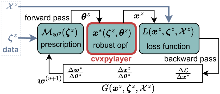
Figure 1: Computation pipeline for the steps itemized in Algorithms 1 and 2. The differentiable optimization layer using cvxpylayers [20], allows the computation of subgradient $G=\nabla_{\bm{w}}L$ with a single backwards pass.

We add the following implementation remarks:

1. Formulation 5 limits the decision variables $\bm{A}$ to the interval $[0,1]$. This leads to $\bm{A}$ taking small values compared to the other decision variables causing conditioning problems in the Cvxpylayers solver ECOS [33]. Introducing a scaling factor for $\bm{A}$ solves this problem consistently.

2. The inner problem has to be always feasible. To ensure this, we add a slack variable to 5b to allow the curtailment of wind power $\bm{u}$ if needed, and a slack variable to 6b to account for the case that the required uncertainty set can not be met with the available reserves. Both sets of slack variables are penalized in the problem objective and conditioned using a scaling factor as in IR1.

3. Formulation 5 is a linear problem and as such may not generally be differentiable with respect to its parameters [34]. This can be avoided by introducing a regularization $\pi\left\lVert\bm{x}\right\rVert_{2}^{2}$ with regularization factor $\pi$ to the objective of the problem. We note that in contrast to [34], our problem is linear with continuous variables and adding a regularization term with a small $\pi$ did not significantly impact our results.

Lastly, we note that we implement $\mathcal{M}_{\bm{w}}$ as two linear models $\mathcal{M}^{\bm{\mu}}=\bm{M}^{\mu}\bm{\zeta}+\bm{m}^{\mu}$ and $\mathcal{M}^{\bm{\sigma}}=\bm{M}^{\sigma}\bm{\zeta}+\bm{m}^{\sigma}$.

IV Numerical Experiments

IV-A Illustrative 5-bus case

We first illustrate the suggested approach using synthetic data on the small-scale “case5” data set from MATPOWER [35]. The system topology with two configurations of wind generators is shown in Fig. 2. Its parameters follow [29] with $\bm{f}^{\rm max}=(3.2,1.52,1.76,0.8,0.8,1.92)$ p.u., $\bm{c}^{\rm E}=(14,15,30,40,10)$$\nicefrac{{\$}}{{MW}}$, and $\bm{c}^{\rm R}=(80,80,15,30,80)$$\nicefrac{{\$}}{{MW}}$.

For training and testing the proposed approach we create a collection of $N=2000$ samples of $\bm{\zeta}=(\bm{d},\bm{u})$ with corresponding samples of $\bm{\xi}$ as follows. First, we define the nominal demand as $\bm{d}_{0}=(0.0,3.0,3.0,4.0,0.0)$ p.u. and the nominal wind forecast as $\bm{u}_{0}=(1.0,1.5)$ p.u.. We then create $N$ samples of $\bm{d}$ by uniformly drawing from the set $\{\bm{d}\in\mathbb{R}\mid 0.5\bm{d}_{0}\leq\bm{d}\leq 1.1\bm{d}_{0}\}$ and $N$ samples of $\bm{u}$ by uniformly drawing from the set $\{\bm{u}\in\mathbb{R}\mid 0.5\bm{u}_{0}\leq\bm{u}\leq 1.1\bm{u}_{0}\}$. Next, for each available sample of $\bm{\zeta}=(\bm{d},\bm{u})$ we draw a sample of forecast errors $\bm{\xi}$ from a multivariate normal distribution with a uniform correlation coefficient of $\phi=0.5$ between all wind farms. Following the observations in [28], we model the forecast error standard deviation to be conditional to the forecast and the forecast error mean to be zero. The resulting normal distribution is given as:

$$\bm{\xi}\,|\,\bm{u}\!\sim\!\mathcal{N}(\bm{0},\bm{\Sigma}_{\bm{u}}),\ \bm{\Sigma}_{\bm{u}}\!=\!\!\begin{bmatrix}(0.15u_{1})^{2}&0.15^{2}\phi u_{1}u_{2})\\ 0.15^{2}\phi u_{1}u_{2})&(0.15u_{2})^{2}\end{bmatrix}\!.$$ (19)

Finally, we set the maximum wind farm capacity to $\bm{u}^{\rm max}=(2.0,3.0)\,\mathrm{p.u.}$ and truncate all generated samples of $\bm{\xi}\,|\,\bm{u}$ such that $\bm{\xi}\geq-\bm{u}$ and $\bm{\xi}\leq\bm{u}^{\rm max}-\bm{u}$. The resulting collection of samples of $\bm{\zeta}$ with a single sample of $\bm{\xi}$ corresponds to what would be available in practice. We use 1500 of these generated samples for training and 500 for testing.

We define the following 5 cases that we use to demonstrate the proposed prescribed robust sets:

• Full: Reference case for which the security interval of each wind farm covers the entire empirical forecast error support.

• 90 Perc: Reference case for which the security interval of each wind farm is fixed between the 10 % and 90 % percentile of the forecast error training data.

• Single: Learning a single fixed uncertainty set without prescription, i.e., $\mathcal{M}^{\mu}=\bm{m}^{\mu}$ and $\mathcal{M}^{\sigma}=\bm{m}^{\sigma}$.

• P-All: Learning $\bm{w}$ using all available forecast errors. As a result, the training is ignorant to the error distribution being conditional to $\bm{u}$.

• P-Cond: Learning $\bm{w}$ assuming access to samples from the true conditional distribution. In each step $z$, given $\bm{u}^{z}$, we generated 200 new samples of $\bm{\zeta}$ using 19.

• P-Bins: Learning $\bm{w}$ with each set of forecast error samples $\mathscr{X}^{z}$ obtained by separating the available training samples of $\bm{u}$ into 10 bins of equal width, as in [28], collecting the forecast error of each bin, and assigning each sample $\bm{u}^{z}$ the set of forecast error samples corresponding to its bin.

We set $v^{\rm max}=100$, although we typically observed satisfying convergence within 40 iterations. We used a mini-batch size of $z^{\rm max}=20$ and a learning rate of $\tau=10^{-6}$. Finally, we set $\bm{w}^{\rm init}$ such that all entries of $\bm{M}^{\mu}$, $\bm{M}^{\sigma}$, and $\bm{m}^{\mu}$ are zero and the entries $\bm{m}^{\sigma}$ correspond to two times the empirical standard deviation of the training data. All experiments are implemented in Python (see also Section III-C) and available online [36]. We used a standard PC workstation with 16 GB memory and an Intel i5 processor.

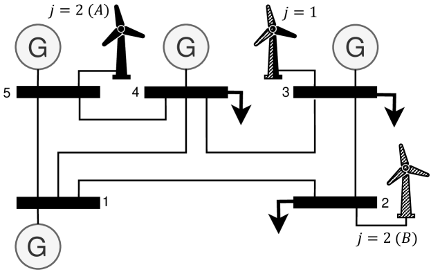
Figure 2: Schematic of the 5 bus test system in configuration A (wind farms at buses 3 and 5) and B (wind farms at buses 2 and 3).

IV-A1 Cost-based box uncertainty set

We first train $\mathcal{M}_{\bm{w}}$ to optimize the expected cost of constraint exceedance (see Section III-A). We set $c_{k}^{\rm viol}=20k\,\mathrm{\nicefrac{{\$}}{{MW}}},\ \forall k$, which corresponds to the lower end of the value of lost load estimated by New York ISO [37]. The average computation time for each epoch across all cases was around 0.25 s, including sampling, solving the inner optimization problems, computing the loss function, and obtaining the gradients.

Fig. 3 shows the out-of-sample (OOS) average cost for the studied cases. The fully robust approach (Full) is overly conservative, which we can infer from the fact that the lowest cost on this case are around the 25-percentile of all other cases. Also, it is often infeasible, leading to higher cost from infeasibility penalties (see Section III-C IR2). The fixed 90 Perc. case is less conservative and mostly avoids infeasibility, but is outperformed by the other cases. The Single uncertainty set improves average cost relative to 90 Perc, but the set remains too small, as it tries to avoid infeasibility penalties. Introducing the prescription step overcomes this problem. The prescriptive cases P-All, P-Cond, and P-Bins further improve upon Single by 12.2 %, 12.7 %, and 10.5 %, respectively. Case P-Cond with access to the true conditional distribution slightly outperforms Single. Case P-Bins performs worse than P-Single, which we attribute to the loss of correlation information in the binning of the forecast errors. Re-running the experiment without correlation ($\phi=0$) confirms this. Now, P-All, P-Cond, and P-Bins result in average OOS cost of 14,899 $, 14,851 $, and 14,981 $, with P-Bins now outperforming P-All and only being slightly worse than the ideal P-Cond.

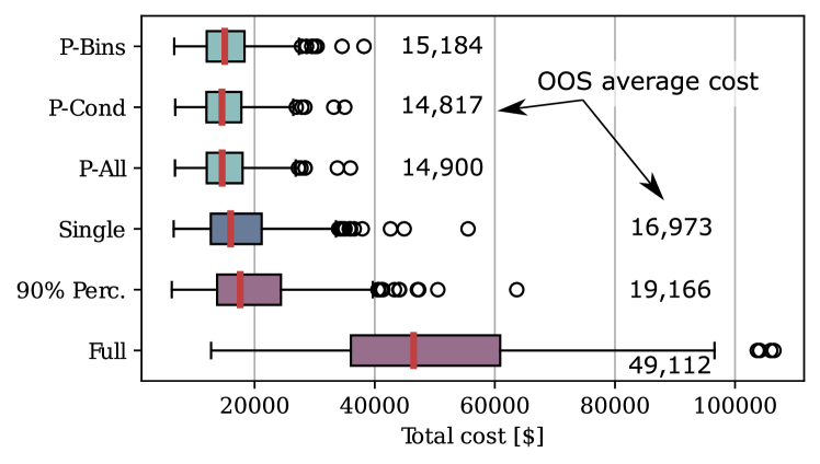
Figure 3: Out-of-sample (OOS) results for 5-bus system in configuration A. Optimized for expected cost of exceedance. The boxes extend from the first quartile to the third quartile. Red line shows the median. The whiskers extend from the box to the farthest data point within 1.5 times the inter-quartile range from the box.

Fig. 4 shows how a change of the system topology impacts the prescribed uncertainty set, highlighting the relevance of making the training problem-aware. By moving wind farm $j=2$ from bus 5 (configuration A) to bus 2 (configuration B), it can no longer rely on the direct balancing from the generator at bus 5. As a result, transmission lines are now more likely to exceed their remaining available margins in real time which leads to larger required safety intervals for both wind farms.

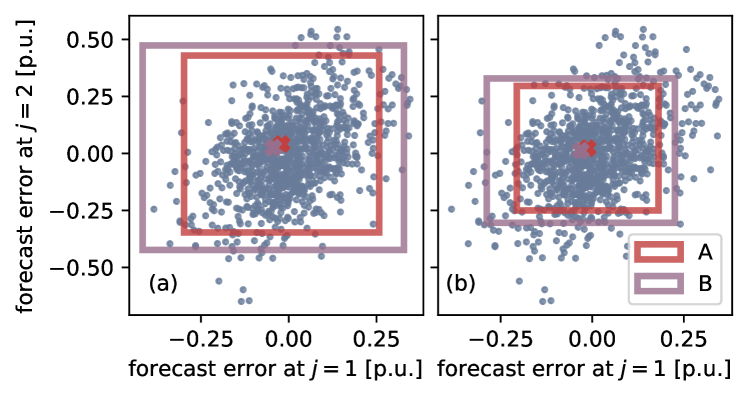
Figure 4: Prescribed sets from case P-All (optimized for cost of exceedance) for (a) $\bm{\zeta}=(\bm{d}_{0},\bm{u}_{0})$ and (b) $\bm{\zeta}=0.7(\bm{d}_{0},\bm{u}_{0})$, each for the two network configurations shown in Fig. 2.

IV-A2 Constraint-based box uncertainty set

We now train $\mathcal{M}_{\bm{w}}$ such that the probability of constraint exceedance remains below 99 %, i.e., $\gamma=0.01$, as described in Section III-B. For this experiment we increase the learning rate to $\phi=10^{-5}$ and set $\lambda^{\rm init}=100$ and $\kappa=0.1$. The time per iteration increased slightly to around 0.67 s per epoch, which we can mainly attribute to the more complex loss function. For Single the CVaR at convergence is 0.96 with an in-training probability of exceedance of 3.1% and a testing probability of exceedance of 13%. As discussed in Section IV-A1 above, this unsatisfying result can be explained with the algorithm avoiding infeasible uncertainty sets resulting in a set that is too small for many parametrizations (see Fig. 5). For P-All, on the other hand, the CVaR at convergence is 0.06 and we achieve an in-training probability of exceedance of 1% and a testing probability of exceedance of 1.8%. We note that the exact match of the in-training probability of exceedance with the target is a coincidence. The actual target of a CVaR equal to zero would lead to a smaller in-training probability of exceedance. However, the algorithm converges above this target as it again tries to avoid to create infeasible sets. Fig. 5 shows the resulting uncertainty sets for Single and P-All and highlights the improved ability of the set in the latter case to adapt to the current system state.

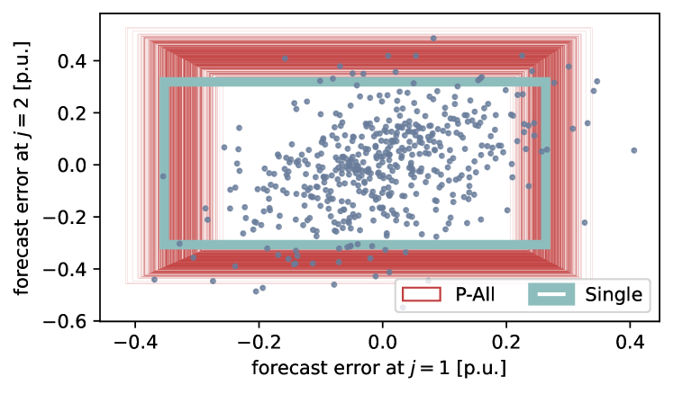
Figure 5: Uncertainty sets for cases P-All and P-Single optimized for probability of exceedance. For P-All all prescriptions resulting from the test samples of $\bm{\zeta}$ are shown. (System configuration A.)

IV-B RTS 96-bus case

We now test the suggested approach on more realistic data using the system provided by the Reliability Test System Grid Modernization Lab Consortium (RTS-GLMC [38]). This update of the RTS-96 test system has 73 buses, 120 transmission lines, 73 conventional generators, 4 wind farms, and 76 other resources (hydro, PV). In our experiment we focus on the 4 wind farms as uncertain resources and treat hydro and PV injections as fixed negative demand, i.e. as part of $\bm{d}$. The RTS-GLMC data set includes data for one year. To have a richer data set for the wind farms, we use the coordinates provided in the RTS-GLMC data set to map the 4 wind farms to the closest data points available in the extensive NREL WIND Toolkit [39]. We scale this data to fit the wind farms in the RTS-GLMC data set and obtain 7 years of wind power injections and realistic forecast errors. We select the data from 2012 to replace the wind data from the RTS-GLMC data set, as the yearly wind structure matches original data most closely (measured in terms of average deviation of hourly total wind injections). From the resulting 8760 available samples net-demand and wind-injection samples of the respective day-ahead data sets, we select 1500 for training and 500 for testing. We use all forecast errors for training as in P-All above and focus on the analysis of the cost of exceedance-based training.

We select the same meta-parameters as for the 5-bus case, but reduce the mini-batch size to $z^{\rm max}=10$. Training requires an average of 28 s per epoch and we observe convergence after around 30 iterations. We note that around half of the time per iteration is spend on computing the gradient. This is expected because both larger parameter matrices $\bm{M}^{\sigma}$, $\bm{M}^{\mu}$ and inner optimization overproportionally increase the size of the computational graph from which the gradient is computed. However, because $\mathcal{M}_{\bm{w}}$ has to be trained only once offline, training time and resources are not a critical limiting factor.

In this case, the reference 90 Perc. leads to a expected out of sample cost of 3,671,312 $ while the P-All trained prescribed sets achieve a significant improvement of 1,249,725 $. (We performed an additional grid search to find a better percentile-based uncertainty set. The best result was attained for the 78-percentile with 3,088,187 $). Fig. 6 shows the OOS forecast errors alongside the collection of prescribed security intervals for the 4 wind farms in the system. We observe that the uncertainty sets are biased towards negative forecast errors. This can largely explained by the fact that the model chooses to curtail wind if the forecast is very high, which (i) leads to an insensitivity to upwards forecast errors and (ii) amplifies the fact that larger negative forecast errors are more likely at high wind power forecasts. This result highlights the advantage of internalizing the problem cost structure into the training.

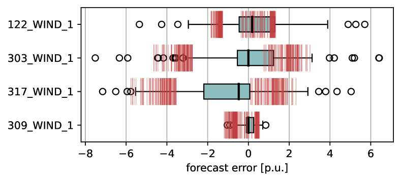
Figure 6: OOS results for the RTS 96 bus case using the P-All training. Box plots show the distribution of the OOS forecast errors and red lines show the various security intervals obtained from the trained mapping. See Fig. 3 for box plot explanation.

V Conclusion

Motivated by the need for actionable methods to deal with stochastic resources in power systems, this paper has demonstrated an approach to compute uncertainty sets for robust optimal power flow that (i) are prescriptive, i.e., minimize the expected cost system cost, and (ii) are adaptive, i.e., are prescribed individually for each expected system state given by a vector of context parameters. Our approach to obtain these sets was inspired by [8] but additionally achieves property (ii).

The problem in 4 opens a wide range of future research [40]. For the approach studied in this paper we are pursuing the following avenues for further research. (i) Including richer context vectors. For example, in our data for the RTS96 case study, we observed a clear dependency of the forecast error distribution on the wind direction. Making the problem more context aware and better estimate conditional error distributions from real data should reveal impactful relations between system security and observable parameters, but is a non-trivial task [40]. (ii) AC power flow. Using a higher fidelity operational model, e.g., along the lines of [2], promises improved applicability in practice and improved system security. (iii) Non-fixed recourse. Relaxing the second stage with a decision-making problem (or a tractable proxy, e.g., a trained neural network), should allow for a broader set of applications of the method. (iv) Improving scalability by utilizing ongoing improvements in differentiable optimization, e.g., [41].

References

- [1] L. Roald and G. Andersson, “Chance-constrained ac optimal power flow,” IEEE Trans. Power Sys., vol. 33, no. 3, pp. 2906–2918, 2017.
- [2] D. Lee et al., “Robust ac optimal power flow with robust convex restriction,” IEEE Trans. Power Sys., vol. 36, no. 6, 2021.
- [3] D. Bienstock et al., “Chance-constrained optimal power flow,” SIAM Review, vol. 56, no. 3, 2014.
- [4] J. Kazempour et al., “A stochastic market design with revenue adequacy and cost recovery by scenario: Benefits and costs,” IEEE Trans. Power Sys., vol. 33, no. 4, pp. 3531–3545, 2018.
- [5] D. Bertsimas et al., “Adaptive robust optimization for the security constrained unit commitment problem,” IEEE Trans. Power Sys., vol. 28, no. 1, pp. 52–63, 2012.
- [6] M. Paturet et al., “Stochastic unit commitment in low-inertia grids,” IEEE Trans. Power Sys., vol. 35, no. 5, pp. 3448–3458, 2020.
- [7] Z. Liang et al., “Inertia pricing in stochastic electricity markets,” IEEE Trans. Power Sys., vol. 38, no. 3, 2022.
- [8] I. Wang et al., “Learning for robust optimization,” arXiv:2305.19225, 2023.
- [9] D. Bertsimas and N. Kallus, “From predictive to prescriptive analytics,” Manag. Sci., vol. 66, no. 3, pp. 1025–1044, 2020.
- [10] J. M. Morales et al., “Prescribing net demand for two-stage electricity generation scheduling,” Oper. Res. Perspect., vol. 10, p. 100268, 2023.
- [11] D. Bertsimas et al., “Data-driven robust optimization,” Math. Program., vol. 167, pp. 235–292, 2018.
- [12] R. Louca and E. Bitar, “Robust ac optimal power flow,” IEEE Trans. Power Sys., vol. 34, no. 3, pp. 1669–1681, 2018.
- [13] F. Golestaneh et al., “Polyhedral predictive regions for power system applications,” IEEE Trans. Power Sys., vol. 34, no. 1, 2018.
- [14] J. M. Morales et al., “Electricity market clearing with improved scheduling of stochastic production,” Eur. J. Oper. Res., vol. 235, no. 3, 2014.
- [15] V. Dvorkin et al., “Setting reserve requirements to approximate the efficiency of the stochastic dispatch,” IEEE Trans. Power Sys., vol. 34, no. 2, pp. 1524–1536, 2018.
- [16] B. Wang and B. F. Hobbs, “Flexiramp market design for real-time operations: Can it approach the stochastic optimization ideal?” in Proceeding of the 2013 IEEE PES Gen. Meeting. IEEE, 2013.
- [17] J. D. Garcia et al., “Application-driven learning: A closed-loop prediction and optimization approach applied to dynamic reserves and demand forecasting,” arXiv:2102.13273, 2021.
- [18] J. Kotary et al., “End-to-end constrained optimization learning: A survey,” arXiv:2103.16378, 2021.
- [19] A. N. Elmachtoub and P. Grigas, “Smart “predict, then optimize”,” Manag. Sci., vol. 68, no. 1, pp. 9–26, 2022.
- [20] A. Agrawal et al., “Differentiable convex optimization layers,” Advances in neural information processing systems, vol. 32, 2019.
- [21] P. Donti et al., “Task-based end-to-end model learning in stochastic optimization,” Adv. Neural Inf. Process., vol. 30, 2017.
- [22] D. Wahdany et al., “More than accuracy: end-to-end wind power forecasting that optimises the energy system,” Electr. Power Syst. Res., vol. 221, p. 109384, 2023.
- [23] V. Dvorkin and F. Fioretto, “Price-aware deep learning for electricity markets,” arXiv:2308.01436, 2023.
- [24] S. Bolognani and F. Dörfler, “Fast power system analysis via implicit linearization of the power flow manifold,” in Proceedings of the 53rd Annual Allerton Conference. IEEE, 2015, pp. 402–409.
- [25] D. Bertsimas et al., “Theory and applications of robust optimization,” SIAM review, vol. 53, no. 3, pp. 464–501, 2011.
- [26] B. L. Gorissen and D. Den Hertog, “Robust counterparts of inequalities containing sums of maxima of linear functions,” Eur. J. Oper. Res., vol. 227, no. 1, pp. 30–43, 2013.
- [27] R. M. Gower et al., “Sgd: General analysis and improved rates,” in Int. Conf. on Machine Learning. PMLR, 2019, pp. 5200–5209.
- [28] Y. Dvorkin et al., “Uncertainty sets for wind power generation,” IEEE Trans. Power Sys., vol. 31, no. 4, pp. 3326–3327, 2015.
- [29] R. Mieth et al., “Data valuation from data-driven optimization,” arXiv:2305.01775, 2023.
- [30] R. T. Rockafellar et al., “Optimization of conditional value-at-risk,” Journal of Risk, vol. 2, pp. 21–42, 2000.
- [31] L. Zhang et al., “Solving stochastic optimization with expectation constraints efficiently by a stochastic augmented lagrangian-type algorithm,” INFORMS Journal on Computing, vol. 34, no. 6, pp. 2989–3006, 2022.
- [32] A. Agrawal et al., “Differentiating through a cone program,” arXiv:1904.09043, 2019.
- [33] A. Domahidi et al., “ECOS: An SOCP solver for embedded systems,” in Proceeding of the European Control Conference, 2013, pp. 3071–3076.
- [34] B. Wilder et al., “Melding the data-decisions pipeline: Decision-focused learning for combinatorial optimization,” in Proceedings of the AAAI Conference on Artificial Intelligence, vol. 33, no. 01, 2019.
- [35] MATPOWER. (2014) CASE5 Power flow data. [Online]. Available: https://matpower.org/docs/ref/matpower5.0/case5.html
- [36] R. Mieth. (2023) Prescribed Robust DC-OPF Code Supplement. [Online]. Available: https://github.com/mieth-robert/p-robust_dcopf
- [37] NYISO, “Ancillary services shortage pricing,” NYISO, Tech. Rep., 2019.
- [38] Reliability Test System - Grid Modernization Lab Consortium. [Online]. Available: github.com/GridMod/RTS-GMLC
- [39] C. Draxl et al., “Overview and meteorological validation of the wind integration national dataset toolkit,” National Renewable Energy Lab. (NREL), Golden, CO (United States), Tech. Rep., 2015.
- [40] U. Sadana et al., “A survey of contextual optimization methods for decision making under uncertainty,” arXiv:2306.10374, 2023.
- [41] J. Kotary et al., “Folded optimization for end-to-end model-based learning,” arXiv:2301.12047, 2023.