Comment
- WoV
- Window of Visibility
- MC
- Monte Carlo
- EMA
- exponential moving average
- pRelMSE
- perceptual relative mean squared error
Perceptual error optimization for Monte Carlo animation rendering
Abstract.
Independently estimating pixel values in Monte Carlo rendering results in a perceptually sub-optimal white-noise distribution of error in image space. Recent works have shown that perceptual fidelity can be improved significantly by distributing pixel error as blue noise instead. Most such works have focused on static images, ignoring the temporal perceptual effects of animation display. We extend prior formulations to simultaneously consider the spatial and temporal domains, and perform an analysis to motivate a perceptually better spatio-temporal error distribution. We then propose a practical error optimization algorithm for spatio-temporal rendering and demonstrate its effectiveness in various configurations.
1. Introduction
Monte Carlo rendering numerically estimates light-transport integrals via random sampling which causes visible noise in the resulting image. Much work has focused on combating this noise by reducing the error in each pixel individually, e.g., via blue-noise or low-discrepancy sampling [Singh et al., 2019]. Applying such a pattern independently within each pixel improves the convergence rate towards a noise-free result. However, the resulting white-noise distribution of error over the image is visually sub-optimal.
It is well understood in digital half-toning literature that the human visual system (HVS) is less sensitive to image error that has high-frequency, i.e., blue-noise, distribution. Georgiev and Fajardo [2016] achieved such distribution in Monte Carlo rendering by carefully optimizing a global sample pattern across image pixels. This pattern yields higher perceptual fidelity by making the pixel estimates as different from each other as possible. This improvement occurs because the HVS applies a low-pass filter to the image [Chizhov et al., 2022], and the negative pixel correlation effectively stratifies the input to the low-pass convolution.
Following the work of Georgiev and Fajardo [2016], several practical methods have been devised to achieve high-quality blue-noise distribution for static-image rendering [Heitz and Belcour, 2019; Belcour and Heitz, 2021; Ahmed and Wonka, 2020]. These are mostly heuristically derived. An exception is the method of Salaün et al. [2022] which leverages the perceptual framework of Chizhov et al. [2022] to compute a small sample set, tiled over the rendered image.
Reusing the same blue-noise sample set across the frames of an animation would maintain good blue-noise distribution, but the noise pattern would remain static over the image. This so-called shower-door effect [Kass and Pesare, 2011] degrades visual quality and disrupts the perception of motion. To address this problem, Wolfe et al. [2022] made a first attempt at obtaining an error distribution for animation rendering that is blue-noise in both image space and time. Lacking firm perceptual grounding, they extend existing blue-noise-mask algorithms to optimize separately across screen-space and time, which leads to visually suboptimal results.
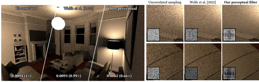
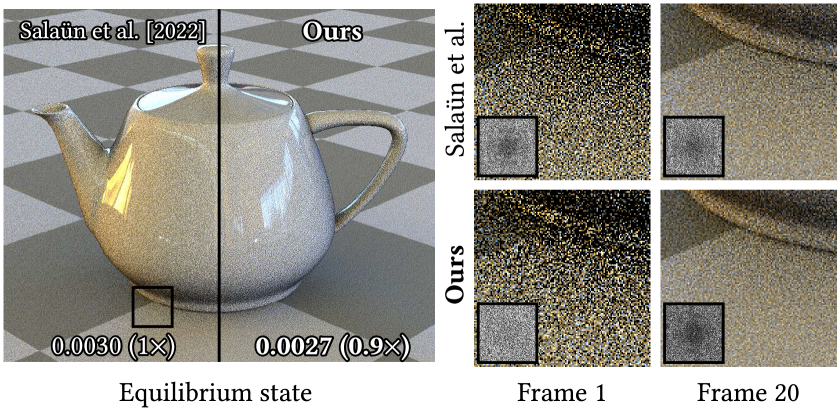
In this paper, we combine the image-space model of Chizhov et al. [2022] with a temporal perception model [Mantiuk et al., 2021] to quantify perceptual error in animation rendering and motivate the need for its high-frequency distribution in both space and time. We also incorporate explicit temporal filtering such as temporal anti-aliasing (TAA). Based on this spatio-temporal model, we adapt the optimization method of Salaün et al. [2022] to obtain scene-independent, precomputed sample sets. The resulting sample sets allow for low-sample animation rendering with higher perceptual fidelity than prior state of the art, thanks to the blue-noise distribution of error in both space and time. Figure 1 shows one frame of an animation rendered with our optimization algorithm.
2. Related work
Our goal is to optimize Monte Carlo rendering error across pixels as blue noise, in both image space and time. The survey of Singh et al. [2019] discusses methods for achieving blue noise on one integration domain (e.g., within a single pixel).
Blue-noise error distribution
Blue-noise distributions of image error appear frequently in dithering or stippling applications [Ulichney, 1988]. The reason for their use is the lower sensitivity of the HVS to high-frequency noise (“blue noise”), resulting in a less perceptible error. High-frequency noise distribution corresponds to negative correlation between pixel values in a neighbourhood. For Monte Carlo rendering, Georgiev and Fajardo [2016] proposed a first practical approach that optimizes a blue-noise sample mask via simulated annealing. Their approach is limited to low-dimensional integration with few samples. Heitz et al. [2019] addressed these limitations by optimizing the scrambling keys of a Sobol sequence [Sobol’, 1967]. Belcour and Heitz [2021] extended this optimization to a rank-1 lattice sampler. The method of Ahmed and Wonka [2020] scrambles an image-space Sobol sequence according to a z-code ordering of pixels to achieve an approximate blue-noise distribution. Salaün et al. [2022] employed sliced optimal transport [Paulin et al., 2020] to obtain a sample set optimized according to the perceptual model of Chizhov et al. [2022]. Recently, Wolfe et al. [2022] proposed extensions to the void-and-cluster [Ulichney, 1988] and Georgiev and Fajardo’s [2016] algorithms to generate blue-noise sample masks for animation rendering. All the aforementioned methods are a priori, i.e., they compute scene-agnostic sample patterns. Such precomputation is beneficial for practical application, though superior quality can be achieved by tailoring the distribution to the specific image being rendered. This can be done through a posteriori adaptation of sample distributions, once the pixels have been sampled [Heitz and Belcour, 2019; Chizhov et al., 2022]. We extend the image-space model of Chizhov et al. [2022] to the temporal domain and apply the a priori optimization approach of Salaün et al. [2022] to acquire a sample pattern for each animation frame.
Perceptual modeling and rendering
The contrast sensitivity function (CSF) is an important characteristic of the HVS that determines the threshold contrast that is perceivable in spatio-temporal signals. A vast majority of CSF measurements focus on spatial patterns [Daly, 1993; Barten, 1999; Wuerger et al., 2020], and the resulting CSFs are modeled by a family of band-pass filters whose parameters change with luminance, color, and retinal eccentricity. Spatio-temporal CSFs have also been derived [Kelly, 1979; Daly, 1998; Robson, 1966; Mantiuk et al., 2022], where temporal sensitivity [de Lange, 1958] can be explained by sustained and transient temporal channels dedicated to processing slowly and quickly changing signals [Burbeck and Kelly, 1980; Hammett and Smith, 1992; Mantiuk et al., 2021]. The so-called window of visibility [Watson, 2013; Watson and Ahumada, 2016; Watson et al., 1986] is an example of such spatio-temporal CSF modeling. The window of visibility approach accounts for spatio-temporal signal processing and sampling that are inherent to any imaging pipeline. In rendering applications, such spatio-temporal CSFs have been used to focus expensive computation on the most visible regions only [Myszkowski et al., 1999; Yee et al., 2001]. In this work, we reduce perceived rendering error by employing a spatio-temporal CSF to optimize space-time sampling patterns.
Temporal anti-aliasing
Temporal anti-aliasing (TAA) combines pixels across multiple frames to reduce noise [Shinya, 1993; Schied et al., 2017, 2018]. Such temporal filtering is simple and cheap, though ghosting artifacts arise if the scene changes too rapidly. These can be reduced via the use of motion vectors or other means of temporal reprojection [Hanika et al., 2021]. Our method can optimize the perceived screen-space error distribution of a TAA-filtered animation.
Bounding integration error
Quasi-Monte Carlo (QMC) integration methods use deterministic sample sequences. These sequences are carefully designed to minimize discrepancy which is a quality metric used to bound integration error [Ermakov and Leora, 2019]. Recent work [Paulin et al., 2020] has shown an analogous error bound based on the Wasserstein distance instead [Kantorovich and Rubinstein, 1958; Villani, 2008]. This bound has been extended by Salaün et al. [2022] to perceptual error in single-image rendering. We further extend their bound to our spatio-temporal setting.
| Notation | Description |
|---|---|
| , | Sample set for frame , sample set for entire frame sequence |
| , | Raw render result at frame , sequence of all raw results |
| , | Displayed image at frame , sequence of all displayed images |
| , | Ground-truth image at frame , sequence of all ground truths |
| , | Perceptual-error image at frame , perceptual-error sequence |
| , | Spatial perceptual kernel, temporal perceptual kernel |
| Explicit temporal accumulation (TAA) kernel | |
| Sample distribution (typically uniform) |
3. Spatio-temporal perceptual model
Our method builds on the perceptual model of Chizhov et al. [2022], which we extend to include the temporal model of Mantiuk et al. [2021] as well as explicit filtering via temporal anti-aliasing (TAA).
Notation
Given a sequence of rendered images, we aim to minimize their perceived error compared to the sequence of corresponding references . Each image is a function of the sample pattern that is used to render the th frame of an animation. We concisely express the sequence of rendered images as a function of the sequence of sample patterns. Table 1 lists the most commonly used symbols throughout the paper.
Spatial perceptual error
We follow Chizhov et al. [2022] and model spatial perceptual response as a convolution. Hence the perceived error of the th frame viewed individually,
| (1) |
can be quantified by comparing the perceived image to the perceived reference . Here, is an image-space Gaussian kernel that approximates the human visual system’s (HVS) point spread function (PSF) [Chizhov et al., 2022]. The error image then measures the error for each pixel in the th frame.
Spatio-temporal perceptual error
The human visual system (HVS) does not perceive each animation frame in isolation. Rather, it has been observed that temporal perception can be also modelled as a low-pass filter [Mantiuk et al., 2021; Burbeck and Kelly, 1980; Hammett and Smith, 1992]. We incorporate temporal filtering with a kernel into the spatial model (1):
| (2) |
Since both reference and rendered images are subject to temporal perception, the convolution with this kernel is applied to both. Here, denotes the sequence of per-frame error images. In our experiments, we employ the kernel proposed by Mantiuk et al. [2021]. It is a sum of two components, a sustained kernel and a transient kernel, plotted in the inline figure. The sustained kernel encodes
![[Uncaptioned image]](/html/2310.02955/assets/x2.png)
Temporal anti-aliasing
TAA methods [Yang et al., 2020] compute pixel values as the weighted average of the current and previous frames. Such explicit filtering can be included in our model by expressing the image displayed at each frame as a convolution of the raw rendering results at all (past) frames: . Substituting into Eq. 2, the error-image sequence becomes
| (3) |
In our experiments, we use an exponential moving average (EMA) kernel , with weights , for , where is a smoothing parameter (we use ). Note here that the perceptual kernels and are applied to both the image estimates and the reference image, but the TAA kernel is applied only to the raw image estimates.
Optimization objective
Our objective is then to find the sample sequence that minimizes the norm of the error-image sequence (3):
In our optimization algorithm, presented in the following section, we use the norm, i.e., we find the sample sequence that minimizes the sum of absolute values of all error-image pixels over all frames.
Discussion
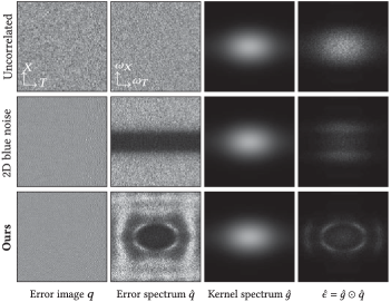
We illustrate the impact of spatio-temporal kernel filtering in Fig. 2, which provides a visual representation of the error image for three different methods, i.e., sample sequences (rows). The first column shows temporal slices of the raw error, i.e., , and the second column shows the power spectra of the discrete Fourier transform (DFT) of those raw-error slices. The last column shows the DFT spectra of the convolution of the error images with our spatio-temporal perceptual kernel (plotted in the second last column). Assuming that the viewing conditions and frame rate correspond to the kernels and , our spatio-temporal kernel approximates the window of visibility [Watson et al., 1986]. This window is defined in the frequency domain and its size is determined by the cut-off spatio-temporal frequencies. Signal outside the window is considered invisible (imperceptible). By optimizing the sample sequence to solve Eq. 4, we not only reduce the magnitude of the spectrum, but also push the energy outside the window of visibility as much as possible. This reduces the residual perceived error for all visible spatio-temporal frequencies.
In summary, in this section we have presented a perception-driven model (3) to assess the spatio-temporal quality of a sample sequence. We model human perception by a series of convolutions, and (optionally) include explicit temporal filtering (TAA). In our main results we use this objective for a priori sample optimization, as discussed in the next section. Figure 5 shows that a posteriori optimization can benefit from this formulation, too.
Similarly to prior work on spatial-only error optimization [Heitz et al., 2019; Heitz and Belcour, 2019; Chizhov et al., 2022], we assume integrated (radiance) function to be locally smooth (Lipschitz continuous) in space and time. This smoothness assumption is essential for achieving a desirable outcome in the optimization process. The spatio-temporal CSF [Kelly, 1979; Daly, 1998; Mantiuk et al., 2022] further supports our assumption since the HVS is mostly sensitive towards low- to mid-frequency signals. In practice, this implies that the sampling quality is less relevant in regions where the smoothness assumption is not met.
4. A priori optimization
Our optimization problem (4) is similar in structure to that of Chizhov et al. [2022] who consider single-image optimization. This problem can be tackled in a priori or a posteriori manner (see Section 2). We focus on a priori optimization due to its higher practical value of computing a sample set once that can be used on any scene. To that end, we extend the method of Salaün et al. [2022] to our spatio-temporal setting.
A priori methods assume that the ground-truth image is constant [Georgiev and Fajardo, 2016; Heitz and Belcour, 2019; Belcour and Heitz, 2021]. We extend this assumption to the temporal domain. Convolving with the TAA kernel thus becomes a no-op that allows us to simplify our objective function (3): we combine all kernels into a single spatio-temporal kernel :
| (5) |
In the a priori setting, both the raw sequence and reference sequence are unknown, preventing the exact minimization of the error (5). Instead, we aim to minimize an upper bound of that error.
Perceptual-error bound
Under our perceptual model, the value of the th pixel in the th frame of the perceived raw sequence is an average of the responses of all samples, weighted by the kernel centered at . Salaün et al. [2022, Appendix D] derived a bound for the absolute error of weighted integral estimates, based on filtered optimal transport. In our case their bound reads
| (6) |
The bound assumes a smooth rendering function, i.e., the incident radiance on the continuous image plane, with Lipschitz constant . It is an integral over Wasserstein distances between the optimized sample distribution and the target (uniform) distribution ; these distributions are filtered to only include the mass at locations where the kernel value exceeds the threshold [Salaün et al., 2022]:
| (7) |
We use the 2-Wasserstein distance which is defined as
| (8) |
Here is the set of all possible transport plans between the two distributions [Bonnotte, 2013]. Since the regular Wasserstein distance is difficult to compute, we further bound it via its sliced variant which involves only easy-to-compute 1D Wasserstein distances [Pitié et al., 2005]:
| (9) |
where and are the projection of the sample set and the uniform density along the 1D line . We provide more details on the Wasserstein error bound in Section 1 of the supplemental document.
To bound the 1-norm of our objective function (5), we sum the error bounds Eq. 6 of all pixels in all frames :
Gradient-descent optimization
We minimize Eq. 10 via stochastic gradient descent, using Monte Carlo integration to estimate the involved integrals. We found that the Adam optimizer works best for our case, due to the sparse support of the kernels and the rather high noise of the gradient estimates. Details on the gradient computation can be found in supplemental Section 2.
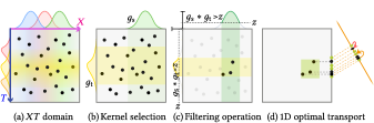
The process is illustrated in Fig. 3. At each optimization step, we first randomly select a kernel (Fig. 3b). We then sample a filtering threshold which yields a sample subset (Fig. 3c). Finally, a random slice is sampled to estimate the gradient of the sliced Wasserstein distance (Fig. 3d). This process is repeated multiple times to reduce the variance. The resulting multi-sample gradient estimate is then used to perform one gradient-descent update step. Algorithm 1 summarizes these optimization steps.
5. Results
We evaluate the rendering performance of our method by computing ray-traced direct illumination with PBRTv3 [Pharr et al., 2016]. We compare the results to the previous approach of Wolfe et al. [2022], independent per-frame spatial-only blue noise [Salaün et al., 2022], and the baseline of independent, white-noise sampling. Animations were rendered at 60Hz. Rendering is done using 1 sample per pixel unless stated otherwise.
We compute fixed-resolution spatio-temporal sample tiles, by toroidally wrapping the kernels during the optimization to ensure that they can be seamlessly tiled in space and time during rendering. If a spatial or temporal kernel has theoretically infinite support, we truncate it at the point where its values become negligible. We observe that a tile needs to be at least an order of magnitude larger than the truncated kernel to avoid tiling artifacts (supplemental, Fig. 1). In our experiments, the kernel size is 77 pixels and 8 frames wide (i.e., 778 pixels). We found that a tile size of 12812830 pixels achieves the best trade-off between optimization cost and tiling artifacts. We use the same tile size for all methods.
We computed the blue-noise tiles of Wolfe et al. [2022] using their public code. We slightly increased their spatial Gaussian kernel to a standard deviation of 2.1 (from 1.9), to match the spatial kernel used for all other methods. We used the public code of Salaün et al. [2022] to generate 30 independently optimized 2D blue-noise sample sets.
To mimic temporal perception in a static image, the renderings presented in the following are temporally pre-filtered with the kernel of Mantiuk et al. [2021] (see Section 3). The visual quality of the results is best appreciated by referring to the supplemental video and HTML viewer.
For quantitative comparison, we compute the perceptual relative mean squared error (pRelMSE), , at the th frame. That is, we filter the rendered image and the reference according to our model (3) and compute the relative MSE of the result for the desired frame (th frame, unless stated otherwise).
We apply our method to animation rendering with and without temporal anti-aliasing (TAA). For our method we optimize on sample set for each variant, tailored to the filter. Table 2 summarizes our quantitative results across a diverse set of test scenes. It shows the pRelMSE of our method and previous works [Salaün et al., 2022; Wolfe et al., 2022] relative to uncorrelated (i.e., white-noise) spatio-temporal sampling. Across all scenes, our method consistently achieves better results, both with and without TAA.
| Scene | Salaün et al. [2022] | Wolfe et al. [2022] | Ours | |||
|---|---|---|---|---|---|---|
| TAA | no TAA | TAA | no TAA | TAA | no TAA | |
| Chopper | 0.61 | 0.62 | 0.69 (0.66) | 0.72 (0.69) | 0.48 | 0.55 |
| Teapot | 0.65 | 0.63 | 0.80 (0.63) | 0.78 (0.65) | 0.56 | 0.58 |
| Modern Hall | 0.90 | 0.85 | 0.98 (0.95) | 0.94 (0.91) | 0.87 | 0.83 |
| Living room | 0.87 | 0.82 | 0.89 (0.86) | 0.86 (0.82) | 0.84 | 0.80 |
| Dragon | 0.54 | 0.52 | 0.66 (0.62) | 0.67 (0.63) | 0.48 | 0.51 |
| Veach MIS | 0.87 | 0.83 | 0.99 (0.97) | 0.92 (0.90) | 0.72 | 0.69 |
Direct viewing
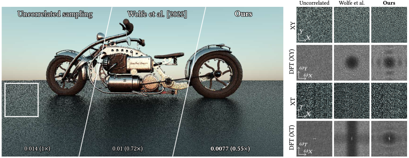
Figures 1 and 6 show results for animations without TAA using 1 sample per pixel. To aid interpretation of the results, the figures display the discrete Fourier transform (DFT) of different zoom-ins. Especially on the temporal slice in the bottom right of Fig. 1, these show clearly where the improvements of our method stem from: While the previous approach of Wolfe et al. [2022] explicitly optimizes for 2D blue noise in image space and 1D blue noise along the temporal domain, our method optimizes samples for an exact kernel, dictated by a perception model. Consequently, the frequency distribution of the error with our method better matches the filter, resulting in a lower perceived error.
Our algorithm can be used to optimize sample sets for any number of samples per pixel. Figure 7 shows an example using four samples. Compared to previous work, our approach achieves a better blue-noise distribution also at higher sample counts.
Temporal anti-aliasing
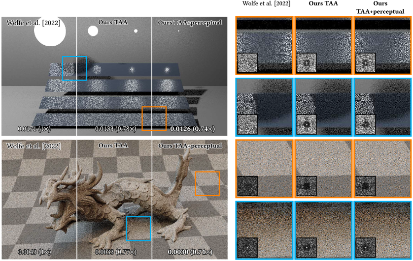
The behavior with explicit TAA filtering is similar to that under direct viewing. Again, our method is consistently better than uncorrelated sampling, previous work [Wolfe et al., 2022], and independent 2D blue noise [Salaün et al., 2022] across all test scenes (Table 2). Figure 9 shows the TAA (and perception) filtered frames of two scenes. For our method, we compare two different optimization objectives: our full model and a simplified version where we left out the perception filter and only optimized for TAA. Optimizing only for TAA still outperforms previous work, but yields 5-10% higher perceived error than utilizing the full model. This supports our hypothesis that optimizing for a more accurate kernel yields best results.
6. Discussion
Impact of kernel shape
Our method differs from that of Wolfe et al. [2022] in two main aspects: the model and the optimization process. The approach of Wolfe et al. [2022] does not directly translate to a kernel in our optimization framework, since they separate the spatial and temporal dimensions. Therefore, to better understand how much of our improvements are due to the model, and how much due to the optimization itself, we performed an ablation where we optimized sample sets for kernels different from the one used for final filtering.
Table 3 summarizes the results. We report the error values for three different kernels: a symmetric Gaussian (standard deviation 2.1), the TAA kernel, and the full TAA and temporal perception kernel [Mantiuk et al., 2021]. As expected, the best result is achieved when optimizing for the full model. Since the TAA and Gaussian kernels have similar shape, their results only differ by a few percent. These results indicate that, while matching the overall shape of the final kernel is important, exact match is not critical.
Note that all models in Table 3 yield lower error than the approach of Wolfe et al. [2022]. This indicates that their separation into spatial and temporal components, while helpful for convergence in their optimizer, hampers the attainable quality.
| Scene | Gaussian | TAA | Perception + TAA |
|---|---|---|---|
| Chopper | 0.75 | 0.75 | 0.70 |
| Teapot | 0.78 | 0.76 | 0.70 |
| Modern Hall | 0.92 | 0.90 | 0.89 |
| Living room | 0.97 | 0.96 | 0.95 |
| Dragon | 0.79 | 0.77 | 0.72 |
| Veach MIS | 0.77 | 0.78 | 0.74 |
Performance on the first frames
Our optimization assumes that a sufficient number of past frames are available to apply the full temporal kernel. This is not the case early in an animation, as shown in Fig. 4. The figure compares our result with spatial-only blue noise [Salaün et al., 2022] under environment-map illumination with TAA filtering. In the first frame, spatial-only optimization yields higher quality, since no temporal filtering can yet occur. In subsequent frames, our method performs better. This is also visible in the DFT spectra (insets) where our method has fewer low-frequency error components, i.e., a better blue-noise distribution.
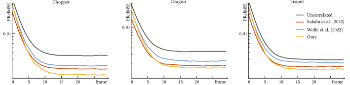
We extend this analysis by comparing the evolution of perceptual error with the number of frames. Figure 8 shows this evolution on the Chopper, Dragon and Teapot scenes. The methods compared are uncorrelated sampling, Salaün et al. [2022], Wolfe et al. [2022] and ours. The results show that at the start of each curve, when few frames are accumulated, spatial-only optimization performs best. This confirms the results presented above. However, as the frames accumulate and the equilibrium state is reached, our method obtains the lowest perceptual error.
A posteriori optimization
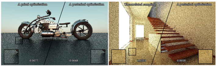
A priori optimization is inherently limited in the achievable quality because the optimized sample set must generalize to arbitrary scenes and importance-sampling transformations. A posteriori optimization can achieve better results, but a truly practical method has yet to be found. To explore the quality achievable by an a posteriori approach using our objective, we extended the method of Chizhov et al. [2022] to the temporal domain, using our model. Specifically, we employ their “vertical” optimization which selects one out of 15 candidate samples for each pixel, to solve Eq. 4. We compare the result to our a priori optimization for the same kernel on the Chopper scene in Fig. 5. Here, a posteriori optimization yields an notable improvement of 60%. These results indicate that further research on (practical) a posteriori methods is worthwhile and can benefit from our formulation.
Optimization cost
Our sample sets need only be computed once per filter kernel, number of integration dimensions, sample count, and frame rate. Nevertheless, when multiple variations of these parameters are desired, computation cost may become a concern. Our CPU implementation takes about 1–2 days to optimize one sample set using 10k SGD steps with a mini-batch size of 4k. The theoretical bottleneck is the computation of the 1D optimal transport, which relies on an sorting operation per gradient-descent iteration. In practice, computation speed is significantly affected by accessing sample subsets that are scattered in memory. Furthermore, the use of a small subset of samples with non-zero gradients per step necessitates the use of large batch sizes, resulting in higher computation costs. Despite these challenges, parallelism can be harnessed within the algorithm: across different projections of the mini-batch on the CPU, also for sorting on the GPU. We believe that, with further performance improvements, e.g., using a pre-optimized set as initialization, computation time can be reduced to at most a few hours per sample set.
Limitations
The signal-constancy assumptions made by a priori perceptual error optimization hold only locally and approximately. In regions of large signal variation, e.g., thin shadow penumbrae (spatially) or fast-moving objects (temporally), perceptual error increases. Temporal variations could be addressed via the use of motion vectors, which we leave for future work.
A significant limitation of a priori optimization methods lies in their applicability to more complex rendering algorithms, such as path tracing. This is due to the increased sampling dimensionality and the variation of the rendering function with longer paths. A priori optimization is not sensitive to dimensionality and can tailor the sampling to the rendered image.
The capacity of the error distribution to influence perceptual quality is also contingent upon the noise level present in the scene. When the noise level is low, the impact of the error distribution on perceptual quality diminishes.
Future work
In this work we use a basic spatio-temporal CSF model [Chizhov et al., 2022; Mantiuk et al., 2021], but our framework (Section 3) supports arbitrary filters. Exploring more advanced CSF models [Mantiuk et al., 2022] that account for display luminance (e.g., darker displays increase the HVS tolerance for contrast errors and flickering, while saving energy) and foveation (sparser sampling with increasing retinal eccentricity) could be a way to further improve visual quality. A hold-type blur of moving objects that arises in the HVS as a function of display persistence and refresh rate [Jindal et al., 2021] can also lead to increasing the HVS tolerance to rendering error. One could specifically optimize sampling by considering content-dependent visual masking [Mantiuk et al., 2021], e.g., by precomputing a texture-specific sample set.
Another promising future direction would be to find a practical approach for a posteriori optimization of sample patterns. Ideally, such a method would work in real-time applications and complex light-transport algorithms.
The relationship between sample optimization and denoising is another interesting topic. As noted by Heitz and Belcour [2019] and Chizhov et al. [2022], high-frequency error distributions can afford higher fidelity when denoising via low-pass filtering; existing denoisers may need adjustment or retraining to optimally handle such input. We believe that our high-frequency spatio-temporal distribution paves the way for devising improved, correlation-aware interactive denoising methods.
7. Conclusion
We have introduced a general model and a practical method for spatio-temporal sample optimization for Monte Carlo animation rendering. Our method accounts for both perceptual and explicit temporal filtering. To achieve practicality, we extend an existing a priori optimization method to support our spatio-temporal model. As a result, we can precompute scene-agnostic sample sets that yield considerable improvements over previous work in terms of perceived noise quality.
Acknowledgements
This project has received funding from the European Union’s Horizon 2020 research and innovation program under Marie Skłodowska-Curie grant agreement №956585. We thank the anonymous reviewers for their feedback, and the authors of the following scenes: julioras3d (Chopper), NewSee2l035 (Modern Hall), Benedikt Bitterli (Utah Teapot), Wig42 (Living Room), and Jay Hardy (White Room).
References
- [1]
- Ahmed and Wonka [2020] Abdalla GM Ahmed and Peter Wonka. 2020. Screen-space blue-noise diffusion of Monte Carlo sampling error via hierarchical ordering of pixels. ACM Transactions on Graphics (TOG) 39, 6 (2020), 1–15.
- Barten [1999] Peter G.J. Barten. 1999. Contrast sensitivity of the human eye and its effects on image quality. SPIE – The International Society for Optical Engineering. https://doi.org/10.1117/3.353254
- Belcour and Heitz [2021] Laurent Belcour and Eric Heitz. 2021. Lessons Learned and Improvements When Building Screen-Space Samplers with Blue-Noise Error Distribution. In ACM SIGGRAPH 2021 Talks (Virtual Event, USA) (SIGGRAPH ’21). Association for Computing Machinery, New York, NY, USA, Article 9, 2 pages. https://doi.org/10.1145/3450623.3464645
- Bonnotte [2013] Nicolas Bonnotte. 2013. Unidimensional and evolution methods for optimal transportation. Ph. D. Dissertation. Paris 11.
- Burbeck and Kelly [1980] Christina A. Burbeck and D. H. Kelly. 1980. Spatiotemporal characteristics of visual mechanisms: excitatory-inhibitory model. J. Opt. Soc. Am. 70, 9 (Sep 1980), 1121–1126. https://doi.org/10.1364/JOSA.70.001121
- Chizhov et al. [2022] Vassillen Chizhov, Iliyan Georgiev, Karol Myszkowski, and Gurprit Singh. 2022. Perceptual error optimization for Monte Carlo rendering. ACM Trans. Graph. 41, 3 (2022). https://doi.org/10.1145/3504002
- Daly [1993] S. Daly. 1993. The Visible Differences Predictor: An Algorithm for the Assessment of Image Fidelity. In Digital Image and Human Vision. 179–206.
- Daly [1998] S. Daly. 1998. Engineering observations from spatiovelocity and spatiotemporal visual models. In Human Vision and Electronic Imaging III. SPIE Vol. 3299, 180–191.
- de Lange [1958] H. de Lange. 1958. Research into the Dynamic Nature of the Human Fovea→Cortex Systems with Intermittent and Modulated Light. I. Attenuation Characteristics with White and Colored Light. J. Opt. Soc. Am. 48, 11 (1958), 777–784.
- Ermakov and Leora [2019] Sergey Ermakov and Svetlana Leora. 2019. Monte Carlo Methods and the Koksma-Hlawka Inequality. Mathematics 7, 8 (2019). https://doi.org/10.3390/math7080725
- Georgiev and Fajardo [2016] Iliyan Georgiev and Marcos Fajardo. 2016. Blue-noise dithered sampling. In ACM SIGGRAPH 2016 Talks. 1–1.
- Hammett and Smith [1992] S.T. Hammett and A.T. Smith. 1992. Two temporal channels or three? A re-evaluation. Vision Research 32, 2 (1992), 285–291. https://doi.org/10.1016/0042-6989(92)90139-A
- Hanika et al. [2021] Johannes Hanika, Lorenzo Tessari, and Carsten Dachsbacher. 2021. Fast Temporal Reprojection without Motion Vectors. Journal of Computer Graphics Techniques Vol 10, 3 (2021).
- Heitz and Belcour [2019] Eric Heitz and Laurent Belcour. 2019. Distributing monte carlo errors as a blue noise in screen space by permuting pixel seeds between frames. In Computer Graphics Forum, Vol. 38. Wiley Online Library, 149–158.
- Heitz et al. [2019] Eric Heitz, Laurent Belcour, Victor Ostromoukhov, David Coeurjolly, and Jean-Claude Iehl. 2019. A low-discrepancy sampler that distributes monte carlo errors as a blue noise in screen space. In ACM SIGGRAPH 2019 Talks. 1–2.
- Jindal et al. [2021] Akshay Jindal, Krzysztof Wolski, Karol Myszkowski, and Rafał K. Mantiuk. 2021. Perceptual Model for Adaptive Local Shading and Refresh Rate. ACM Trans. Graph. 40, 6, Article 281 (2021).
- Kantorovich and Rubinstein [1958] Leonid V. Kantorovich and Gennady S. Rubinstein. 1958. On a space of completely additive functions. Vestnik Leningrad Univ 13 7 (1958), 52–59.
- Kass and Pesare [2011] Michael Kass and Davide Pesare. 2011. Coherent noise for non-photorealistic rendering. ACM Transactions on Graphics (TOG) 30, 4 (2011), 1–6.
- Kelly [1979] D.H. Kelly. 1979. Motion and Vision 2. Stabilized Spatio-Temporal Threshold Surface. Journal of the Optical Society of America 69, 10 (1979), 1340–1349.
- Mantiuk et al. [2022] Rafał K. Mantiuk, Maliha Ashraf, and Alexandre Chapiro. 2022. StelaCSF: A Unified Model of Contrast Sensitivity as the Function of Spatio-Temporal Frequency, Eccentricity, Luminance and Area. ACM Trans. Graph. 41, 4, Article 145 (2022).
- Mantiuk et al. [2021] Rafał K Mantiuk, Gyorgy Denes, Alexandre Chapiro, Anton Kaplanyan, Gizem Rufo, Romain Bachy, Trisha Lian, and Anjul Patney. 2021. FovVideoVDP: A visible difference predictor for wide field-of-view video. ACM Transactions on Graphics (TOG) 40, 4 (2021), 1–19.
- Myszkowski et al. [1999] K. Myszkowski, P. Rokita, and T. Tawara. 1999. Perceptually-Informed Accelerated Rendering of High Quality Walkthrough Sequences. In Proc. EGSR. 5–18.
- Paulin et al. [2020] Lois Paulin, Nicolas Bonneel, David Coeurjolly, Jean-Claude Iehl, Antoine Webanck, Mathieu Desbrun, and Victor Ostromoukhov. 2020. Sliced optimal transport sampling. ACM Trans. Graph. 39, 4 (2020), 99.
- Pharr et al. [2016] Matt Pharr, Wenzel Jakob, and Greg Humphreys. 2016. Physically based rendering: From theory to implementation. Morgan Kaufmann.
- Pitié et al. [2005] François Pitié, Anil C. Kokaram, and Rozenn Dahyot. 2005. N-Dimensional Probablility Density Function Transfer and its Application to Colour Transfer. In 10th IEEE International Conference on Computer Vision. IEEE Computer Society. https://doi.org/10.1109/ICCV.2005.166
- Robson [1966] John Robson. 1966. Spatial and Temporal Contrast-Sensitivity Functions of the Visual System. Journal of The Optical Society of America 56 (08 1966). https://doi.org/10.1364/JOSA.56.001141
- Salaün et al. [2022] Corentin Salaün, Iliyan Georgiev, Hans-Peter Seidel, and Gurprit Singh. 2022. Scalable Multi-Class Sampling via Filtered Sliced Optimal Transport. ACM Trans. Graph. 41, 6, Article 261 (nov 2022), 14 pages. https://doi.org/10.1145/3550454.3555484
- Schied et al. [2017] Christoph Schied, Anton Kaplanyan, Chris Wyman, Anjul Patney, Chakravarty R Alla Chaitanya, John Burgess, Shiqiu Liu, Carsten Dachsbacher, Aaron Lefohn, and Marco Salvi. 2017. Spatiotemporal variance-guided filtering: real-time reconstruction for path-traced global illumination. In Proceedings of High Performance Graphics. 1–12.
- Schied et al. [2018] Christoph Schied, Christoph Peters, and Carsten Dachsbacher. 2018. Gradient estimation for real-time adaptive temporal filtering. Proceedings of the ACM on Computer Graphics and Interactive Techniques 1, 2 (2018), 1–16.
- Shinya [1993] Mikio Shinya. 1993. Spatial Anti-Aliasing for Animation Sequences with Spatio-Temporal Filtering. In Proc. SIGGRAPH 93. 289–296.
- Singh et al. [2019] Gurprit Singh, Cengiz Öztireli, Abdalla G.M. Ahmed, David Coeurjolly, Kartic Subr, Oliver Deussen, Victor Ostromoukhov, Ravi Ramamoorthi, and Wojciech Jarosz. 2019. Analysis of Sample Correlations for Monte Carlo Rendering. Computer Graphics Forum 38, 2 (2019), 473–491. https://doi.org/10.1111/cgf.13653 arXiv:https://onlinelibrary.wiley.com/doi/pdf/10.1111/cgf.13653
- Sobol’ [1967] I.M Sobol’. 1967. On the distribution of points in a cube and the approximate evaluation of integrals. U. S. S. R. Comput. Math. and Math. Phys. 7, 4 (1967), 86–112. https://doi.org/10.1016/0041-5553(67)90144-9
- Ulichney [1988] R.A. Ulichney. 1988. Dithering with blue noise. Proc. IEEE 76, 1 (1988), 56–79. https://doi.org/10.1109/5.3288
- Villani [2008] C. Villani. 2008. Optimal Transport: Old and New. Springer Berlin Heidelberg. https://books.google.fr/books?id=hV8o5R7_5tkC
- Watson [2013] Andrew B Watson. 2013. High frame rates and human vision: A view through the window of visibility. SMPTE Motion Imaging Journal 122, 2 (2013), 18–32.
- Watson and Ahumada [2016] Andrew B Watson and Albert J Ahumada. 2016. The pyramid of visibility. Electronic Imaging 2016, 16 (2016), 1–6.
- Watson et al. [1986] Andrew B. Watson, Albert J. Ahumada, and Joyce E. Farrell. 1986. Window of visibility: a psychophysical theory of fidelity in time-sampled visual motion displays. J. Opt. Soc. Am. A 3, 3 (1986), 300–307.
- Wolfe et al. [2022] Alan Wolfe, Nathan Morrical, Tomas Akenine-Möller, and Ravi Ramamoorthi. 2022. Spatiotemporal Blue Noise Masks. In Eurographics Symposium on Rendering. https://doi.org/10.2312/sr.20221161
- Wuerger et al. [2020] Sophie Wuerger, Maliha Ashraf, Minjung Kim, Jasna Martinovic, María Pérez-Ortiz, and Rafał K. Mantiuk. 2020. Spatio-chromatic contrast sensitivity under mesopic and photopic light levels. Journal of Vision 20, 4 (04 2020), 23–23. https://doi.org/10.1167/jov.20.4.23
- Yang et al. [2020] Lei Yang, Shiqiu Liu, and Marco Salvi. 2020. A Survey of Temporal Antialiasing Techniques. Computer Graphics Forum 39, 2 (2020), 607–621. https://doi.org/10.1111/cgf.14018 arXiv:https://onlinelibrary.wiley.com/doi/pdf/10.1111/cgf.14018
- Yee et al. [2001] Hector Yee, Sumanita Pattanaik, and Donald P. Greenberg. 2001. Spatiotemporal Sensitivity and Visual Attention for Efficient Rendering of Dynamic Environments. ACM Trans. Graph. 20, 1 (2001), 39–65.