f(R) Gravity in an Ellipsoidal Universe

Abstract

We propose a new model of cosmology based on an anisotropic background and a specific $f(R)$ theory of gravity. It is shown that field equations of $f(R)$ gravity in a Bianchi type I background give rise to a modified Friedmann equation. This model contains two important parameters: $\gamma$ and $\delta$. We, thus, simply call our model $\gamma\delta$CDM. It is distinguished in two important aspects from the $\Lambda$CDM model: firstly, the contribution of different energy densities to the Hubble parameter are weighted with different weights, and then, dependence of energy densities to redshift is modified as well. This unorthodox relation of energy content to Hubble parameter brings forth a new way of interpreting the cosmological history. This solution does not allow the existence of a cosmological constant component, however, a dark energy contribution with dependence on redshift is possible. We tested observational relevance of the new solution by best fitting to different data sets. We found that our model could accommodate the idea of cosmological coupling of black holes.

I Introduction

Advances in cosmology in both observational and theoretical fronts in the last decades were immense and these theoretical and the observational advancements supported each other to build the highly successful “standard model” of cosmology, so called $\Lambda$CDM model. Under the assumptions of isotropy and homogeneity of matter distribution in the Universe, and the validity of Einstein’s theory of gravity at all classical scales, the $\Lambda$CDM model brings theoretical explanation to observations in both the late and the early universe. Scientific explanation, however, is never complete and scientific progress accelerates after inconsistencies in the paradigm itself start to appear and new ideas are begin to be explored in order to resolve those inconsistencies.

In cosmology, first of all, there is an important inconsistency between numerically fitted value of the Hubble constant to the late and the early universe data. The discrepancy is on the order of $5\sigma$ Abdalla:2022yfr ; Shah:2021onj ; Freedman:2021ahq and it has been called a “crisis” Verde:2019ivm . Whereas Hubble constant is calculated from the Cosmic Microwave Background (CMB) data with a theoretical input Planck:2018vyg , it is been fitted to the late universe observational data independent of any cosmological model Riess:2021jrx ; Pesce:2020xfe ; Freedman:2019jwv ; Wong:2019kwg ; Birrer:2018vtm ; Dominguez:2019jqc ; LIGOScientific:2017adf ; Moresco:2017hwt . Since these discrepancy is not resolved in $\Lambda$CDM model yet Abdalla:2022yfr ; Shah:2021onj ; DiValentino:2021izs ; Perivolaropoulos:2021jda ; Schoneberg:2021qvd ; Knox:2019rjx , it is plausible to seek alternative theoretical explanations to the observational data. One avenue of research has been to change the third assumption of the standard cosmology, namely that the theory of gravitation could be different than the Einstein’s theory on scales larger than at least the scale of the Solar System.

One of the simplest modifications of the Einstein’s theory of gravity is the $f(R)$ theory of gravity (see reviews Sotiriou:2008rp ; DeFelice:2010aj ; Nojiri:2010wj ; Nojiri:2017ncd and references therein). Action of this theory includes an arbitrary function of the scalar curvature R and in that aspect it is different than the Einstein-Hilbert action, which depends on the scalar curvature itself. There are many works on the cosmological implications of $f(R)$ gravity since Starobinsky’s seminal paper Starobinsky:1979ty ; Starobinsky:1980te ; Vilenkin:1985md . In the present work we are going to present a new solution to the field equations of $f(R)$ gravity in the anisotropic Bianchi type I background geometry Collins:1973lda . The fact that we work in an anisotropic background is motivated by the “anomalies” Buchert:2015wwr ; Schwarz:2015cma in the observational data both in the early and the late universe. An anisotropic universe under the influence of Einstein gravity with a positive cosmological constant tends to isotropize asymptotically Starobinsky:1962 ; Wald:1983ky . In the case of $f(R)$ gravity, however, it is possible to have anisotropically expanding cosmological solutions Barrow:2005qv . This is the reason we aim to find a theoretical explanation to the anomalies and inconsistencies in the current cosmological model with an anisotropic background solution in the $f(R)$ theory of gravity.

CMB data explicitly includes anomalies that hint the existence of a global anisotropy. These were persistently observed by the COBE COBE:1992syq ; Kogut:1996us , WMAP Bennett:2010jb ; deOliveira-Costa:2003utu ; WMAP:2003ivt ; WMAP:2003zzr ; WMAP:2003elm and Planck experiments Planck:2015igc ; Planck:2019kim . Among these anomalies the most well known is the lack of power in the quadrupole moment in the CMB power spectrum Planck:2018vyg ; Buchert:2015wwr ; Schwarz:2015cma ; Campanelli:2006vb ; Cea:2022mtf ; Campanelli:2007qn ; Cea:2019gnu . Other than that the quadrupole and octupole moments are observed to be aligned with each other and the motion of the solar system, even though they are expected to be independent of each other Copi:2013jna ; Land:2005ad ; Schwarz:2004gk . Additionally there is an observed power asymmetry between northern and southern hemispheres of our chosen celestial sphere Planck:2019evm ; Mukherjee:2015mma ; Javanmardi:2016whx ; Axelsson:2013mva ; Eriksen:2007pc , and there exists so called cold spots on the microwave sky Vielva:2003et ; Cruz:2006sv . Each of these anomalies in data might have different reasons and might require different physical solutions. However they might also be collectively pointing out the existence of a preferred direction in space Schwarz:2015cma ; Cea:2022mtf ; Luongo:2021nqh ; Krishnan:2021jmh ; Rodrigues:2007ny ; Bridges:2007ne ; Migkas:2020fza . There are further hints of anisotropy in the Pantheon supernova data from the late Universe Pan-STARRS1:2017jku ; Mohayaee:2021jzi ; Zhao:2019azy ; Amirhashchi:2018nxl ; Colin:2019opb ; Colin:2010ds . Such an anisotropic background geometry might be captured by Bianchi type metrics, simplest of which is the Bianchi type I metric Campanelli:2006vb ; Cea:2022mtf ; Campanelli:2007qn ; Cea:2019gnu ; Akarsu:2019pwn ; Akarsu:2020pka ; Akarsu:2021max ; Tedesco:2018dbn ; Amirhashchi:2018bic ; Hossienkhani:2014zoa ; Nojiri:2022idp . We will not treat $f(R)$ gravity field equations in the anisotropic Bianchi type I background geometry as effective Einstein equations Capozziello:2005mj ; Nojiri:2006ri ; Capozziello:2006dj ; Faraoni:2018qdr . Thus the solution will relate the Hubble parameter to the energy content of the universe very differently compared to the standard general relativistic formalism. Our solution contains two important parameters: $\gamma$ and $\delta$. We, thus, simply call our model $\gamma\delta$CDM.

One of the important aspects of the new solution is that the contribution of different energy densities to the Hubble parameter are weighted with different weights. Other than that, dependence of energy densities to redshift is also modified. This unorthodox relation of the energy content to the Hubble parameter brings forth a new way of interpreting the cosmological history. Our solution does not allow existence of a cosmological constant component, however a dark energy contribution with dynamical dependence on redshift is possible. We test the observational relevance of the $\gamma\delta$CDM model by best fitting to different data sets, such as the Pantheon type Ia supernovae data Pan-STARRS1:2017jku , the cosmic chronometers (CC) Hubble data Jimenez:2001gg ; Favale:2023lnp and the Baryon Acoustic Oscillations (BAO) data Akarsu:2019pwn of the late universe, and the CMB data Planck:2018vyg of the early universe.

The important difference between the $\gamma\delta$CDM model and the $\Lambda$CDM model manifests itself in the best fit value of the dark energy density, $\Omega_{e0}$. From the data fit analysis with the above data sets we find that the best fit value for the dark energy density, $\Omega_{e0}$, is just a few percent of the universe’s total energy. We note that such a low value for the density of dark energy could be explained with the cosmological coupling of black holes Croker:2021duf ; Farrah:2023opk ; Croker:2020plg . We find that the best fit value of $(3-k)$, where $k$ is called cosmological coupling constant, inferred by comparing supermassive black holes in five samples of elliptical galaxies at $z>0.7$ to those in contemporary elliptical galaxies Farrah:2023opk is well within the 1$\sigma$ regions of the $\gamma$ parameter for all combinations of the data sets. This whole line of argument has a theoretical basis put forward long time ago by Gliner Gliner:1966 , who argues that the state of collapsed matter in a black hole interior can be considered as a source of dark energy with negative pressure and $p+\rho\geqslant 0$.

This paper is organized as follows: in the next section we will present the action and the field equations of the $f(R)$ gravity. Afterwards, we will write the field equations in terms of the Hubble and the shear anisotropy parameters in the Bianchi type I background. Then, under the assumption that the matter content can be approximated by a perfect fluid, the shear anisotropy parameter will be shown to obey a Gauss-Codazzi type equation. After obtaining redshift dependence of shear anisotropy parameter, subsequent solution of the field equations will provide us a new solution of the Hubble parameter in terms of the energy content of the universe. In section III we are going to present the data sets with which we will test our solution and summarize the data fitting method that is used. In section IV we will present and discuss the relevance of the results of the data fit analysis. Lastly in section V we will summarize our work and comment on our results.

II Theory

II.1 f(R) theory of gravity

The action of $f(R)$ gravity depends on an arbitrary function of the scalar curvature $R$. In such a theory total action can be written as

$$S=-\int d^{4}x\sqrt{-g}\left(\frac{1}{2\kappa}f(R)+\mathcal{L}_{m}\right)$$ (1)

where $\mathcal{L}_{m}$ denotes the Lagrangian density for matter fields and $\kappa=8\pi G$ is the Einstein’s constant in the natural units (c=1).

The field equations of $f(R)$ gravity can be obtained by varying the action with respect to the metric. They are given by

$$f_{R}R_{\mu\nu}-\frac{1}{2}fg_{\mu\nu}+\left(g_{\mu\nu}\Box-\nabla_{\mu}\nabla_{\nu}\right)f_{R}=\kappa T_{\mu\nu}$$ (2)

where $T_{\mu\nu}=-\frac{2}{\sqrt{-g}}\frac{\delta\mathcal{S}_{m}}{\delta g_{\mu\nu}}$ is the energy-momentum tensor, and $f_{R}=\frac{\partial f}{\partial R}$.

II.2 Ellipsoidal Universe

On the hypothesis that the quadruple anomaly in CMB data could be due to existence of a preferred direction in space, we adopt an ellipsoidal model of the Universe as in Campanelli:2006vb ; Campanelli:2007qn ; Cea:2019gnu . This model is described by a Bianchi type I metric, which is simply given by

$$ds^{2}=-dt^{2}+A(t)^{2}dx^{2}+B(t)^{2}(dy^{2}+dz^{2})\,,$$ (3)

where directional scale parameters $A(t)$ and $B(t)$ are different from each other. Directional Hubble parameters are defined as $H_{x}=\dot{A}/A$ and $H_{y}=H_{z}=\dot{B}/B$. Physical volume is given by $V(t)=A\cdot B^{2}$ and we define an average scale parameter $a(t)$ by the relation $V(t)=a(t)^{3}$.

We then define two new parameters in terms of the directional Hubble parameters as

$$H(t)=\frac{1}{3}(\frac{\dot{A}}{A}+2\frac{\dot{B}}{B})\quad\mathrm{and}\quad S(t)=\frac{\dot{A}}{A}-\frac{\dot{B}}{B}\,.$$ (4)

Here $H(t)$ is the average Hubble parameter and we call $S(t)$ the shear anisotropy parameter. $S^{2}(t)$ is related to so called shear scalar $\sigma^{2}(t)$ that quantifies the anisotropic expansion Leach2006 by $S^{2}(t)=3\sigma^{2}(t)$. Scalar curvature of Bianchi type I spacetime (3) is given by

$$R=12H^{2}+6\dot{H}+\frac{2}{3}S^{2}\,.$$ (5)

We further express the Hubble parameter in terms of the average scale parameter $a(t)$ as $H(t)=\dot{a}/a$, which is the usual relation.

Instead of expresssing the field equations in terms of the metric functions $A(t)$ and $B(t)$ we are going to utilize the Hubble and the anisotropy parameters. In terms of $H(t)$ and $S(t)$ the field equations are

$$\mathrm{(00)} : f_{R}\left(3H^{2}+3\dot{H}+\frac{2S^{2}}{3}\right)-\frac{1}{2}f-3f_{RR}H\dot{R}=-\kappa\rho\,,$$ (6)

$$\mathrm{(11)} : f_{R}\left(3H^{2}+2HS+\dot{H}+\frac{2\dot{S}}{3}\right)-\frac{1}{2}f-f_{RR}\left[(2H-\frac{2}{3}S)\dot{R}+\ddot{R}\right]-f_{RRR}\dot{R}^{2}=\kappa p\,,$$ (7)

$$\mathrm{(22)} : f_{R}\left(3H^{2}-HS+\dot{H}-\frac{\dot{S}}{3}\right)-\frac{1}{2}f-f_{RR}\left[(2H+\frac{1}{3}S)\dot{R}+\ddot{R}\right]-f_{RRR}\dot{R}^{2}=\kappa p\,,$$ (8)

where we approximated the matter content as a perfect fluid. This means that there are no anisotropic pressure components and therefore the left hand sides of $(11)$ and $(22)$ field equation components should be the same. In these equations we have $f_{RR}=\frac{\partial^{2}f}{\partial R^{2}}$ and $f_{RRR}=\frac{\partial^{3}f}{\partial R^{3}}$. $(33)$ component of the field equations is the same as the $(22)$ component, thus it is not written.

Combining the equations (7) and (8) we obtain

$$0=f_{R}S\left(3\frac{\dot{a}}{a}+\frac{\dot{S}}{S}\right)+f_{RR}S\dot{R}\,,$$ (9)

which is equivalent to the trace free Gauss-Codazzi equation Leach2006 ; Banik2016 given by

$$\frac{\dot{S}}{S}=-\left[3\frac{\dot{a}}{a}+\frac{\dot{f}_{R}}{f_{R}}\right]$$ (10)

Assuming that the shear anisotropy parameter has the time dependence such as

$$\dot{S}=-\varepsilon HS$$ (11)

one can easily solve equation (10) and determine $f_{R}=\frac{\partial f}{\partial R}$ and $S(t)$ as a function of the scale parameter $a(t)$ as

$$f_{R}=\frac{\varphi}{a^{3-\varepsilon}}\quad and\quad S=\frac{s_{0}}{a^{\varepsilon}}\,,$$ (12)

where $\varphi$ and $s_{0}$ are the integration constants.

Under the condition (9) the field equations become

$$\kappa\rho = -f_{R}\left(3H^{2}+3\dot{H}+\frac{2S^{2}}{3}\right)+\frac{1}{2}f+3H\dot{f}_{R}\,,$$ (13)

$$\kappa p = f_{R}\left(3H^{2}+\dot{H}\right)-\frac{1}{2}f-2H\dot{f}_{R}-\ddot{f}_{R}\,.$$ (14)

II.3 Solution to the field equations

According to the analysis done in Leach2006 and Maartens:1994pb the contribution of shear to the Hubble parameter would be expected to be different than the case in general relativity. In $f(R)$ theory, the contribution of shear to the Hubble parameter comes due to $2S^{2}/3$ term in (13). In general relativity shear dissipates as $S^{2}\propto a^{-6}$. In contrast, for example, in the $f(R)=R+\alpha R^{2}$ theory shear is expected to be dissipated more slowly compared to general relativity Maartens:1994pb . Thus we expect parameter $\varepsilon$ of (11) to be less than three so that $S^{2}$ dissipates slower than its general relativistic analogue. So we choose that

$$\varepsilon=3-\delta\quad\mathrm{with}\quad 0<\delta<1$$ (15)

This chosen range of $\delta$ is consistent with the dynamical systems analysis and equation (60) of Leach2006 .

We assume that the Hubble parameter has a polynomial dependence on the scale parameter $a$ as

$$H^{2}=\sum_{\lambda}\frac{h_{\lambda}}{a^{\lambda}}\,,$$ (16)

where $\lambda\in\mathbb{R}$ are to be determined from the field equations (13 & 14).

We can now solve the function $f(R)$ in terms of the average scale parameter $a$ by using the relations (12) and the form of the scalar curvature R (5) in terms of $a$. We find $f(a)$ to have the form

$$f(a)=\varphi\sum_{\lambda}\frac{\lambda(12-3\lambda)}{\lambda+\delta}\frac{h_{\lambda}}{a^{\lambda+\delta}}+\varphi\frac{4(3-\delta)}{3(6-\delta)}\frac{s_{0}^{2}}{a^{6-\delta}}-2\Lambda,$$ (17)

where $2\Lambda$ is an integration constant.

We further assume that there are the usual relativistic and non-relativistic perfect fluid components of the energy density and pressure. Non-relativistic component is the dust (m) with vanishing pressure. Relativistic component is composed of a positive pressure radiation (r) component and a negative pressure dark energy (e) component. We find that the field equations (13 & 14) do not allow a cosmological constant to be a part of $f(R)$ theory, but dark energy component could have equation of state parameter $\omega=\gamma/3-1$ with $0<\gamma\leq 2$. Thus the total energy density and pressure of perfect fluids are given by

$$\rho=\frac{\rho_{e0}}{a^{\gamma}}+\frac{\rho_{m0}}{a^{3}}+\frac{\rho_{r0}}{a^{4}}\quad\mathrm{and}\quad p=(\frac{\gamma}{3}-1)\frac{\rho_{e0}}{a^{\gamma}}+\frac{1}{3}\frac{\rho_{r0}}{a^{4}}\,,$$ (18)

where $\rho_{e0},\rho_{m0}$ and $\rho_{r0}$ are the present day dark energy, non-relativistic matter (dust) and relativistic matter (radiation) densities, respectively.

Substituting relations (12, 17 & 18) into the field equations we are able to determine possible $\lambda\in\mathbb{R}$ values and solve the Hubble parameter in terms of the perfect fluid densities as

$$3H^{2}=\frac{\kappa\rho_{e}}{\varphi b_{\gamma}}\frac{1}{a^{\gamma-\delta}}+\frac{\kappa\rho_{m}}{\varphi b_{3}}\frac{1}{a^{3-\delta}}+\frac{\kappa\rho_{r}}{\varphi b_{4}}\frac{1}{a^{4-\delta}}+\frac{1}{3}\frac{s_{0}^{2}}{1-\delta}\frac{1}{a^{6-2\delta}}\,,$$ (19)

where coefficients $b_{n}$ ($n=\gamma,3,4$) are given by

$$b_{n}=-\left(1+\delta-\frac{1}{2n}(n-\delta)(4+\delta)\right)\,.$$ (20)

Coefficient $b_{0}$ is divergent unless $\delta=0$, which is the case of general relativity. Therefore we cannot include a cosmological constant term into this model, and thus we take integration constant in the relation (17) to be vanishing.

To compare theoretical form of the Hubble parameter with the observational data we express $H^{2}$ in terms of dimensionless density parameters as

$$H^{2}=\frac{H_{0}^{2}}{\varphi}\left[\frac{\Omega_{e0}}{b_{\gamma}}\frac{1}{a^{\gamma-\delta}}+\frac{\Omega_{m0}}{b_{3}}\frac{1}{a^{3-\delta}}+\frac{\Omega_{r0}}{b_{4}}\frac{1}{a^{4-\delta}}+\frac{\Omega_{s0}}{1-\delta}\frac{1}{a^{6-2\delta}}\right]\quad\mathrm{with}\quad\Omega_{s0}=\frac{\varphi s_{0}^{2}}{9H_{0}^{2}}\,.$$ (21)

where $\Omega_{s0}$ gives the present day contribution of anisotropic shear to the Hubble parameter and $H_{0}$ is the Hubble constant at the present time. Other dimensionless present day density parameters ($\Omega_{e0}$ for dark energy, $\Omega_{m0}$ for dust and $\Omega_{r0}$ for radiation) are defined by dividing respective densities with the critical density $\rho_{c}=3H_{0}^{2}/8\pi G$.

The general relativistic limit is obtained as $\delta\rightarrow 0$ and $\varphi\rightarrow 1$. In that case we find that $b_{\gamma}=b_{3}=b_{4}=1$ and that $\Omega_{e0}+\Omega_{m0}+\Omega_{r0}+\Omega_{s0}=1$ as it should be for a flat universe described by general relativity and Friedmann equations. We also note that in the same limit shear dissipates with the sixth power of the average scale parameter ($a^{-6}$) as is expected in the general relativistic case.

For the sake of simplicity we will not have $\varphi$ as a free parameter and take $\varphi=1$ also in the general $f(R)$ case when we compare our solution with the cosmological data. A non-vanishing $\delta$ parameter makes all the important difference between these theory and the general relativity. Value of $\delta$ parameter determines both the contribution of different perfect fluid components to the expansion of the Universe and also how these components are dissipates as the Universe expands. Coefficients $b_{n}$ for $n=\gamma,3,4$ depend on the value of $\delta$ and they weight the contributions of different $\Omega_{i}$ to the Hubble parameter. Depending on the value of $\delta$ the contribution of one component may get enhanced as the contribution of another component is diminished.

Another important effect of non-zero value of $\delta$ is that even though perfect fluid components diminish with expansion depending on their physical nature, their contributions to the expansion diminishes differently. For example dust (non-relativistic matter) component diminishes with $a^{3}$, but its contribution to the expansion diminishes slower with $a^{3-\delta}$. The same also is true for the other perfect fluid components. Their contributions to the Hubble parameter diminishes slower than their actual physical dynamics requires.

Faster dependence on the scale parameter was observed in solutions to the field equations of Brans-Dicke theory with non-zero Brans-Dicke parameter $\omega_{BD}$ in the case of a flat isotropic universe in Boisseau:2010pd and a flat anisotropic universe in Akarsu:2019pvi . As is well known, Brans-Dicke theory with a kinetic term for the auxiliary scalar field is not equivalent to any f(R) theory Velasquez:2018euw . Thus, the theories of gravity studied in those works are completely different from the theory we study here. Both of these works have exact solutions if the perfect fluid is only composed of non-relativistic pressureless fluid, i.e., dust, and also both of them cannot include the radiation component in the exact analytical solution and can only include “effective” dark energy. Thus, these models Boisseau:2010pd ; Akarsu:2019pvi are some unrealistic solutions in the Brans-Dicke framework. Additionally, in these works, the dust component’s contribution to the Hubble parameter diminishes faster than its actual physical dynamics requires. This is in complete contrast with what we have here in the f(R) theory framework.

This way, the theory has an enhanced ability to adjust itself to fit with different data sets from completely different cosmological eras. It is obvious that existence of the parameters $\delta$ and $\gamma$ cause the essential difference of this model with the $\Lambda$CDM or related anisotropic $\Lambda$CDM models Akarsu:2019pwn ; Akarsu:2021max . Therefore we call this model simply as $\gamma\delta$CDM model. In the rest of this paper we are going to summarize the data analysis and check the expectations of the $\gamma\delta$CDM model (21) with various cosmological data sets.

III Data and Methodology

III.1 Data

To constrain our parameters in the theoretical model with the observations we use the latest and most relevant data sets. The following four data sets are distinct both in the physical origin and the observational methodology:

1. CC Hubble data: The latest compilation of data obtained through the cosmic chronometers method Jimenez:2001gg comprise 32 data points which are given in Table 1 (see references therein) with low redshift ($0.07<z<1.97$). These redshift values are the same in Favale:2023lnp ; however, the values of H(z) are taken from those calculated by the BC03 model for the redshifts, which are mentioned in Moresco:2012 ; Moresco:2015 ; Moresco:2016 .

   For the data points taken from Moresco:2012 ; Moresco:2015 ; Moresco:2016 there are contributions to the model covariance matrix due to the uncertainties due to star formation history, the IMF, the stellar library, and the stellar population synthesis model. Detailed information and the way we follow the calculation of the covariance matrix is the same as in Moresco:2020 . The rest of the data points in Table 1 are uncorrelated with the data taken from Moresco:2012 ; Moresco:2015 ; Moresco:2016 , and, therefore, we include them diagonally in the covariance matrix.

   The chi-squared function for the 32 H(z) measurements, denoted by $\chi^{2}_{CC}$, is defined as

   $$\chi^{2}_{CC}=M^{T}Cov^{-1}M,$$ (22)

   where M represents the residual between model prediction $H^{th}(z_{i})$ and observational data $H^{obs}(z_{i})$ as

   $$M=H^{obs}(z_{i})-H^{th}(z_{i})\ .$$ (23)

   $z_{i}$	$H^{obs}(z_{i})\pm\sigma(z_{i})$	References
   0.07	69 $\pm$ 19.6	Zhang:2014 Zhang et al. (2014)
   0.09	69 $\pm$ 12	Jimenez:2003 Jimenez et al. (2003)
   0.12	68.6 $\pm$ 26.2	Zhang:2014 Zhang et al. (2014)
   0.17	83 $\pm$ 8	Simon:2005 Simon et al. (2005)
   0.1791	74.91 $\pm$ 3.8	Moresco:2012 Moresco et al. (2012)
   0.1993	74.96 $\pm$ 4.9	Moresco:2012 Moresco et al. (2012)
   0.2	72.9 $\pm$ 29.6	Zhang:2014 Zhang et al. (2014)
   0.27	77 $\pm$ 14	Simon:2005 Simon et al. (2005)
   0.28	88.8 $\pm$ 36.6	Zhang:2014 Zhang et al. (2014)
   0.3519	82.78 $\pm$ 13.94	Moresco:2012 Moresco et al. (2012)
   0.3802	83 $\pm$ 13.54	Moresco:2016 Moresco et al. (2016)
   0.4	95 $\pm$ 17	Simon:2005 Simon et al. (2005)
   0.4004	76.97 $\pm$ 10.18	Moresco:2016 Moresco et al. (2016)
   0.4247	87.08 $\pm$ 11.24	Moresco:2016 Moresco et al. (2016)
   0.4497	92.78 $\pm$ 12.9	Moresco:2016 Moresco et al. (2016)
   0.47	89 $\pm$ 49.6	Ratsimbazafy:2017 Ratsimbazafy et al. (2017)
   0.4783	80.91 $\pm$ 9.044	Moresco:2016 Moresco et al. (2016)
   0.48	97 $\pm$ 62	Stern:2010 Stern et al. (2010)
   0.5929	103.8 $\pm$ 12.49	Moresco:2012 Moresco et al. (2012)
   0.6797	91.6 $\pm$ 7.96	Moresco:2012 Moresco et al. (2012)
   0.75	98.8 $\pm$ 33.6	Borghi:2022 Borghi et al. (2022)
   0.7812	104.5 $\pm$ 12.19	Moresco:2012 Moresco et al. (2012)
   0.8754	125.1 $\pm$ 16.7	Moresco:2012 Moresco et al. (2012)
   0.88	90 $\pm$ 40	Stern:2010 Stern et al. (2010)
   0.9	117 $\pm$ 23	Simon:2005 Simon et al. (2005)
   1.037	153.7 $\pm$ 19.67	Moresco:2012 Moresco et al. (2012)
   1.3	168 $\pm$17	Simon:2005 Simon et al. (2005)
   1.363	160 $\pm$ 33.58	Moresco:2015 Moresco (2015)
   1.43	177 $\pm$ 18	Simon:2005 Simon et al. (2005)
   1.53	140 $\pm$ 14	Simon:2005 Simon et al. (2005)
   1.75	202 $\pm$ 40	Simon:2005 Simon et al. (2005)
   1.965	186.5 $\pm$ 50.43	Moresco:2015 Moresco (2015)

   Table 1: Cosmic Chronometers Hubble Data. $H^{obs}(z_{i})\pm\sigma(z_{i})$ is in $km/s/Mpc$.

2. CMB data: The first peak of the CMB spectrum, denoted by $l_{\ast}$, is called the angular scale of the sound horizon at the last scattering surface and is given by

   $$l_{\ast}=\pi\frac{D_{M}(z_{\ast})}{r_{\ast}}\ ,\quad\mathrm{with}\quad D_{M}(z_{\ast})=c\int_{0}^{z_{\ast}}\frac{dz}{H(z)}$$ (24)

   as the comoving angular diameter distance to the last scattering surface and $r_{\ast}$ is the size of the comoving sound horizon. Both are calculated at the last scattering surface with redshift $z_{\ast}=1089.9$ Planck:2018vyg .

   According to both the Planck 2015 and 2018 CMB data Planck:2015 ; Planck:2018vyg , $l_{\ast}=301.63$ is observed with uncertainty $\sigma_{l_{\ast}}=0.15$. The chi-squared function of CMB that can be written in the light of this information is

   $$\chi^{2}_{CMB}=\frac{(l_{\ast}^{obs}-l_{\ast}^{th})^{2}}{\sigma_{l_{\ast}}^{2}}$$ (25)

3. BAO data: We use BAO measurements by 6dFGS, MGS, BOSS LOWZ, SDSS(R), BOSS CMASS and WiggleZ surveys as summarized in table 3 of Akarsu:2019pwn comprising 8 data points with low redshift ($0.106<z<0.73$). Even though these are observations form the late universe, they carry information from the redshift at the baryon drag epoch ($z_{d}=1059.6$). Below we only state differences in our analysis compared to Akarsu:2019pwn .

   The baryon acoustic oscillations are density fluctuations of the visible baryonic matter. The BAO measurements constrain the ratio of the comoving size of the sound horizon to the dilation scale:

   $$d^{th}(z)=\frac{r_{d}}{D_{v}(z)}\ .$$ (26)

   In this ratio, $r_{d}=r_{s}(z_{d})$ is the comoving size of the sound horizon at the drag redshift, $z_{d}=1059.6$:

   $$r_{s}(z_{d})=\int_{z_{d}}^{\infty}\frac{c_{s}}{H(z)}dz\ ,$$ (27)

   where $c_{s}=\frac{c}{\sqrt{3(1+R/(1+z))}}$ is the sound speed in the photon-baryon fluid and $R/(1+z)=3\rho_{b0}/(4\rho_{r0})$ is the ratio of baryon to photon momentum density Eisenstein:1997 ; Wang:Yun . Given the observed average temperature of the CMB, $T_{CMB}=2.728K$, the value of $R$ is given by $R=31500\Omega_{b}h^{2}(T_{CMB}/2.7K)^{-4}$ with $\Omega_{b}h^{2}=0.02226$ Planck:2015 .

   The dilation scale, $D_{v}(z)$, is a combination of the radial dilation and the transverse dilation, given by Eisenstein:1997 ; SDSS:2005xqv

   $$D_{v}(z)=\left[D_{M}(z)^{2}\frac{cz}{H(z)}\right]^{\frac{1}{3}}$$ (28)

   where $D_{M}(z)$ is the comoving angular diameter distance at redshift z.

   The total chi-squared function for BAO measurements is given in terms of two separate contributions:

   $$\chi_{BAO}^{2}=\chi_{W}^{2}+\chi_{NW}^{2}$$ (29)

   First one is the chi-squared function for the WiggleZ dark energy survey, calculated utilizing a covariance matrix and the second chi-squared function is for the other five surveys as explained in Akarsu:2019pwn .

4. SnIa data: The data we use to test our cosmological model are taken from Pan-STARRS1:2017jku . The magnitude data samples of Type Ia Supernovae (SnIa) consist of PS1, SDSS, SNLS, Low-z, and Hubble Space Telescope (HST) data samples ranging $0.01<z<2.3$. There are a total of 1048 SnIa measurements and are called ”Pantheon samples.” All these data can be found in the web site Scolnic:data and github repositories of Scolnic:pant .

   We use the magnitude data of SnIa to constrain our cosmological model parameters. Observations of SnIa measure the apparent magnitude of supernovae which we call as $m$. We follow the reference Conley:2011 and use the same theoretical model to describe the apparent magnitude of SnIa. The model is given in terms of the distance modulus called $\mu$ as follows:

   $$m=\mu+M,$$ (30)

   where $M$ is the absolute magnitude of SnIa. We take this model as simplified version of Conley:2011 ; Betoule:2014 with vanishing color-luminosity and stretch-luminosity parameters.

   The chi-squared function for the Patheon data is given by

   $$\chi^{2}=\Delta m^{T}C^{-1}\Delta m\ ,$$ (31)

   where $\Delta m=m_{B}-m$ and $C$ is the covariance matrix taken from Pan-STARRS1:2017jku . $m_{B}$ is the measured values of apparent B-band magnitude of SnIa.

   The absolute magnitude $M$ depends on the dynamics of SnIa. Since it is a parameter that is independent of the cosmological model and measured uncertainties of individual SnIa, we removed it out of the statistical analysis by using the methods described in Conley:2011 . After removing absolute magnitude $M$, we use the chi-squared function as given in appendix C of Conley:2011 to constrain the parameters in our cosmological model with the Pantheon SnIa data.

III.2 Methodology

In this work we use the Bayesian inference method for parameter estimation and model comparison Padilla:2019 ; Hogg:2010 . Bayes theorem is a consequence of the probability axioms. If $x_{1}$ and $x_{2}$ are two mutually exclusive events, the probability of both events occurring is equal to the product of the probability of $x_{1}$ and the probability of $x_{2}$ given that $x_{1}$ has already happened:

$$P(x_{1}\cap x_{2})=P(x_{1})P(x_{2}|x_{1})$$ (32)

This is also true other way around and gives us,

$$P(x_{1}|x_{2})=\frac{P(x_{2}|x_{1})P(x_{1})}{P(x_{2})}.$$ (33)

The equation above can be converted for a given model $\mathcal{M}$, the data $I$ and the parameters $\theta$ in Bayesian inference as

$$P(\theta|\mathcal{I},\mathcal{M})=\frac{P(\mathcal{I}|\theta,\mathcal{M})P(\theta|\mathcal{M})}{P(\mathcal{I}|\mathcal{M})}\ ,$$ (34)

where $P(\theta|\mathcal{I},\mathcal{M})$ is called the posterior probability of a given model $\mathcal{M}$. $P(\mathcal{I}|\theta,M)=\mathcal{L}(\mathcal{I}|\theta,\mathcal{M})$, which is known as the likelihood function of the model, is given by

$$\mathcal{L}(\mathcal{I}|\theta,\mathcal{M})\propto\exp{\left[-\frac{1}{2}\chi^{2}(\mathcal{I}|\theta,\mathcal{M})\right]}$$ (35)

where $\chi^{2}(\mathcal{I}|\theta,\mathcal{M})$ is the chi-squared function. Thus, the minimum value of the chi-squared function gives the maximum likelihood.

We derive posterior probability distributions and the maximum likelihood function with the nested sampling Monte Carlo algorithm MLFriends Buchner:2014 ; Buchner:2017 using the UltraNest package Buchner:2021 . Nested sampling is a Monte Carlo algorithm that computes an integral over the model parameters. In this work, we tried to constrain model parameters and compare the model to the $\Lambda$CDM model by using the UltraNest.

We calculate the joint chi-squared function of all the data sets as

$$\chi^{2}(\mathcal{I}|\theta,\mathcal{M})=\chi^{2}_{CC}+\chi^{2}_{CMB}+\chi^{2}_{BAO}+\chi^{2}_{SnIa}$$ (36)

Then the likelihood function is multivariate joint Gaussian likelihood given by (35).

The free parameters of our cosmological model are $H_{0},\ \Omega_{m0},\ \Omega_{s0},\ \gamma$ and $\delta$ (21). For $\Omega_{r0}$ we used the value $\Omega_{r0}=h^{-2}.2.469.10^{-5}(1+\frac{7}{8}(\frac{4}{11})^{4/3}N_{eff})$ where $N_{eff}=3.046$ as given in Mukhanov:2005sc determined by the value of CMB temperature and the Stefan-Boltzmann law. We fixed $\Omega_{e0}$ in terms of other parameters at $a(t_{0})=a_{0}=1$ and constrained the remaining five cosmological parameters through the data analysis.

Priors are chosen so as to scan the parameter space throughly and determine the best fit value of the parameters. The uniform prior distributions are chosen for the parameters $H_{0}$ and $\Omega_{m0}$, given by $0.5\leqslant H_{0}\leqslant 0.85$ and $0.0\leqslant\Omega_{m0}\leqslant 1.0$, respectively. For $\Omega_{s0}$ we choose logarithmic prior distribution given by $-16\leqslant\log_{10}\Omega_{s0}\leqslant 0.0$ due to its expected very low value. For the analysis summarized in Table 2 logarithmic prior distribution is chosen for $\gamma$ with $0.001\leqslant\gamma\leqslant 3.0$ and uniform prior distribution is chosen for $\delta$ with $0.0\leqslant\delta\leqslant 0.772$. The corresponding likelihood and contour plots are given in Fig. 1. All plots are produced by GetDist, which is commonly used to analyze Monte Carlo samples Lewis:2019xzd .

In section II we emphasized that in this model the dark energy component cannot be a cosmological constant and thus the parameter $\gamma$ cannot be zero (21). Due to this fact, the lower bound of the prior distribution for $\gamma$ could not be zero, but could be arbitrarily close to zero. Since lower bound could be arbitrarily small, but not zero, we use logarithmic prior distribution for the parameter $\gamma$. We have checked various choices for the lower bound of the prior distribution for $\gamma$ and we find that the median value and the minimum chi-squared function for those fits do not change significantly. In the next section we report the results for minimum $\gamma$ chosen to be $0.001$. The lower bound of the prior distribution for $\delta$ is chosen zero, since this value corresponds to the case of general relativistic solution. The upper bound is chosen to be $\frac{1}{2}(\sqrt{73}-7)\approx 0.772$ because for larger values of $\delta$ the coefficient $b_{3}$ (20) becomes negative, which will render the contribution of the matter density to the expansion of the universe to be negative, which, needless to say, is unphysical.

IV Results and Discussion

We present the constraints with 68% CL on the free ($H_{0},\ \Omega_{m0},\ \Omega_{s0},\ \gamma$ and $\delta$) and some derived parameters ($\Omega_{e0},\Omega_{e0}/b_{\gamma}$ and $\Omega_{m0}/b_{3}$) of the $\gamma\delta$CDM model for different data set combinations in Table 2, and 1D and 2D posterior distributions, with 1$\sigma$ and 2$\sigma$ marginalized confidence regions, for the free parameters in Fig. 1. For comparison we also provide marginalized constraints for the parameters of the $\Lambda$CDM standard model (for which $\delta,\ \gamma$ and $\Omega_{s0}$ all vanish) in Table 2.

Table 2: Constraints, with 68% CL and (best fit) value, on the free ($H_{0},\ \Omega_{m0},\ \Omega_{s0},\ \gamma$ and $\delta$) and some derived parameters ($\Omega_{e0},\Omega_{e0}/b_{\gamma}$ and $\Omega_{m0}/b_{3}$) of the $\gamma\delta$CDM model for different data set combinations. For comparison we also provide constraints on the parameters of the $\Lambda$CDM model (for which $\delta,\ \gamma$ and $\Omega_{s0}$ all vanish) in blue. Minimum values of the chi-squared functions for both models are also presented.

Data set	CC	CC+CMB	CC+CMB+BAO	CC+CMB+BAO+SnIa
Model	$\gamma\delta$CDM	$\gamma\delta$CDM	$\gamma\delta$CDM	$\gamma\delta$CDM
	$\Lambda$CDM	$\Lambda$CDM	$\Lambda$CDM	$\Lambda$CDM
$\mathbf{H_{0}}$	$66.43^{+4.39}_{-4.46}$ (69.37)	$65.48^{+3.76}_{-2.47}$ (69.38)	$68.80^{+2.93}_{-2.60}$ (69.35)	$70.19^{+2.06}_{-2.60}$ (70.46)
	$68.88^{+4.03}_{-4.25}$ (69.43)	$67.81^{+4.00}_{-3.90}$ (68.66)	$70.36^{+0.57}_{-0.58}$ (70.38)	$70.32^{+0.56}_{-0.57}$ (70.34)
$\mathbf{\Omega_{m0}}$	$0.2636^{+0.0813}_{-0.0993}$ (0.3099)	$0.2863^{+0.0894}_{-0.1130}$ (0.3077)	$0.2900^{+0.0183}_{-0.0127}$ (0.2934)	$0.2836^{+0.0109}_{-0.0088}$ (0.2873)
	$0.3171^{+0.0680}_{-0.0543}$ (0.3087)	$0.3092^{+0.0659}_{-0.0532}$ (0.2967)	$0.2738^{+0.0074}_{-0.0071}$ (0.2735)	$0.2743^{+0.0075}_{-0.0072}$ (0.2740)
$\mathbf{\Omega_{s0}}$	$54.97$ ($3.575$) $\cdot 10^{-11}$	$4.535$ ($9.441$) $\cdot 10^{-14}$	$2.642$ ($14.93$) $\cdot 10^{-14}$	1.660 (11.77) $\cdot 10^{-14}$
$\mathbf{\gamma}$	$0.8099^{+0.8647}_{-0.5833}$ (0.01545)	$0.6456^{+0.8649}_{-0.5284}$ (0.04605)	$0.1927^{+0.3548}_{-0.1391}$ (0.2159)	$0.07842^{+0.1061}_{-0.0555}$ (0.05223)
$\mathbf{\delta}$	$0.1194^{+0.1899}_{-0.0953}$ (0.007133)	$0.0170^{+0.0370}_{-0.0135}$ (0.02152)	$0.0121^{+0.0317}_{-0.0086}$ (0.02709)	$0.0105^{+0.0200}_{-0.0079}$ (0.02486)
$\mathbf{\Omega_{e0}}$	0.4411 (0.04919)	0.6644 (0.03393)	0.6127 (0.5115)	0.5177 (0.02092)
$\mathbf{\Omega_{e0}/b_{\gamma}}$	0.6928 (0.6887)	0.7078 (0.6843)	0.7057 (0.6969)	0.7128 (0.7040)
$\mathbf{\Omega_{m0}/b_{3}}$	0.3071 (0.3112)	0.2921 (0.3156)	0.2942 (0.3030)	0.2871 (0.2959)
min $\mathbf{\chi}^{2}$	$14.50$	$14.51$	$20.04$	$172.44$
	$14.50$	$14.96$	$21.02$	$173.22$

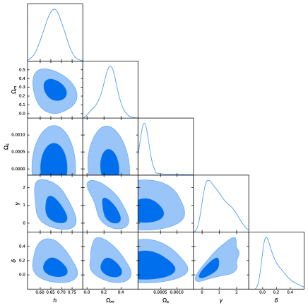
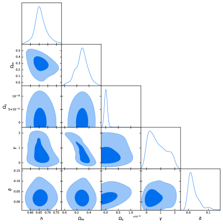
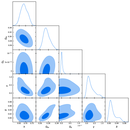
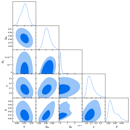
Figure 1: The 1D and 2D posterior distributions with 1$\sigma$ and 2$\sigma$ marginalized confidence regions of model parameters from CC (top-left), CC+CMB (top-right), CC+CMB+BAO (bottom-left), and CC+CMB+BAO+SnIa (bottom-right) data combinations. The Hubble constant $H_{\rm 0}=100\cdot h$ is in units of km/s/Mpc.

As we examine Fig. 1 we note that the posterior distributions for the $\gamma$ and $\delta$ parameters are not Gaussian. Therefore, the mean and the median values for these parameters are quite different than the best fit values (maximum likelihood) as can be observed in Table 2. Other free parameters ($H_{0}$ and $\Omega_{m0}$) do have Gaussian distributions and thus their median values are very close to the best fit values. When we examine the minimum values for the chi-squared functions we observe that in the case of maximum likelihood $\gamma\delta$CDM model is not significantly favored over the $\Lambda$CDM model. One of the important differences of the $\gamma\delta$CDM model from the $\Lambda$CDM can be seen in the difference between the best fitted values of the matter density, $\Omega_{m}$, in the case of $\Lambda$CDM model and the effective matter density, $\Omega_{m0}/b_{3}$, in the case of $\gamma\delta$CDM model. Best fitted values of the effective matter density, $\Omega_{m0}/b_{3}$, are more consistent across the data sets compared to the $\Omega_{m}$ values in $\Lambda$CDM. Likewise, the effective dark energy density, $\Omega_{e0}/b_{\gamma}$, has consistent values across the data sets. We emphasize the important distinction between the dark energy density, $\Omega_{e0}$, and its effect on the expansion of the universe through the term, $\Omega_{e0}/b_{\gamma}$ as given in (21). Unlike in the case of the matter density and the effective matter density, which have approximate values with each other, the dark energy density and the effective dark energy density could be quite different. This difference is especially pronounced in the best fit values of these quantities. Except the data set CC+CMB+BAO, the best fit values of the dark energy density ($\Omega_{e0}$) are found quite low, on the order of a few percent, very much different than the values inferred for the effective dark energy density ($\Omega_{e0}/b_{\gamma}$), which are approximate to the values found for $\Omega_{e0}$ in the $\Lambda$CDM model. Thus this model empowers small amount of dark energy to have big impact on the expansion of the universe. One other interesting point worth emphasizing is the following: the effective densities for the dark energy and the matter, $\Omega_{e0}/b_{\gamma}$ and $\Omega_{m0}/b_{3}$ respectively, have best fit values very close to the best fit values for dark energy and matter densities in $\Lambda$CDM model. Thus even though the true densities could be quite different between the models, their effect on the expansion of the universe is almost the same in the $\gamma\delta$CDM and the $\Lambda$CDM models.

Accepting that the dark energy density, $\Omega_{e0}$, is just a few percent of the universe’s energy bucket, is there an explanation for the origin of such a low value for the density of dark energy? Interestingly, some recent works on the cosmological coupling of black holes Croker:2021duf ; Farrah:2023opk might provide an explanation. Hypothesis of these works is that a black hole’s mass is coupled to cosmological expansion and thus it changes with redshift as

$$M(z)=\Big{(}\frac{1+z_{i}}{1+z}\Big{)}^{k}M(z_{i})\qquad z\leqslant z_{i}\ ,$$ (37)

where $k$ is called cosmological coupling strength and black hole becomes cosmologically coupled at redshift $z_{i}$. It is also claimed in Croker:2020plg that spatial distribution of these black holes as point sources becomes uniform on scales $\lesssim 200$ Mpc. Thus, as the universe expands the density of such a “continuum fluid” will decrease with a rate of $(1+z)^{3}$ Croker:2020plg . Together with the black hole mass growth as given above in (37) the contribution of this continuum fluid to the expansion of the universe will depend on the redshift with the power law $(1+z)^{(3-k)}$. The power $(3-k)$ is equivalent to $\gamma$ in our work (see equation (18)). The best fit value of $(3-k)$, inferred by comparing supermassive black holes in five samples of elliptical galaxies at $z>0.7$ to those in contemporary elliptical galaxies Farrah:2023opk is well within the 1$\sigma$ regions of the $\gamma$ parameter for all combinations of data sets. Thus, our work is in agreement with the claims made in Croker:2021duf ; Farrah:2023opk and Croker:2020plg . This whole line of argument is also in agreement with the theoretical considerations put forward long time ago by Gliner Gliner:1966 . Gliner argues that the gravitational collapse of a star do not end up in a singularity, but the force of gravitational contraction renders the pressure of matter to be negative, which effectively acts to contract the distribution of matter. Thus, the state of collapsed matter in a black hole interior can be considered as a source of dark energy.

V Conclusions

In this work, we investigated the cosmology of an ellipsoidal universe in the framework of $f(R)$ theory of gravity. Although we observe a homogeneous and isotropic universe at scales larger than roughly 100 $Mpc$, there are indications that this was possibly not always the case during the history of the universe. These are the observations that indicate possible anisotropy in the distribution of matter and the geometry of the universe as summarized in the introduction. In the standard cosmological paradigm there are also so called “tensions” of the results from observations of early and late epochs of the universe. The most famous of these are the tensions in the value of the Hubble constant $H_{0}$ and the value of the growth parameter $S_{8}$ (see excellent reviews on cosmological tensions, such as Abdalla:2022yfr ; Shah:2021onj ; Freedman:2021ahq ; Verde:2019ivm ; DiValentino:2021izs ; Perivolaropoulos:2021jda ; Schoneberg:2021qvd ; Knox:2019rjx ). There are many proposals in the literature to resolve these tensions, and the alternative gravity approach is one of them. In the present work we investigated the effect of perhaps the simplest extension of general relativity, namely $f(R)$ gravity on the evolution of the universe. There are many works that examines the evolution of various types of ellipsoidal universes in the general relativistic context, e.g., see Campanelli:2006vb ; Cea:2022mtf ; Campanelli:2007qn ; Cea:2019gnu ; Akarsu:2019pwn ; Akarsu:2020pka ; Akarsu:2021max ; Tedesco:2018dbn ; Amirhashchi:2018bic ; Hossienkhani:2014zoa .

Our work is distinguished from other works on $f(R)$ gravity cosmology in the sense that we do not obtain the Friedmann equation in its general relativistic form. In the alternative gravity cosmologies, the usual approach is to treat the extra terms, which are additional to the general relativistic ones in the field equations, as an effective energy-momentum tensor and this way to obtain so called “curvature” contributions to the various energy densities. Here our approach is quite different. The Friedmann equation is not in the general relativistic form. The consequence of this modified form of the Friedmann equation (21) is enormous. The energy densities do not contribute the expansion of the universe as in the ordinary Friedmann equation. Depending of the value of the $\delta$ parameter (15) the contribution of various energy densities to the Hubble parameter are enhanced or diminished. Existence of the anisotropic stress $\Omega_{s0}$ requires to have the $\delta$ parameter Leach2006 in the theory. Then not just the contribution of various energy densities to the modified Friedmann equation are weighted by the coefficients $b_{n}$ (20), but also their scale factor or redshift dependence shifts (21) by $a^{\delta}=(1+z)^{-\delta}$ compared to the standard formalism Mukhanov:2005sc . Other than these changes we find that this solution of the field equations do not allow a cosmological constant term as part of the $f(R)$ function. Nevertheless, one can consider the possibility of a dark energy term with redshift dependence $(1+z)^{\gamma}$, with $0<\gamma<2$ that originates from the matter Lagrangian. Together with the shift $(1+z)^{-\delta}$, the dark energy term in the modified Friedmann equation depends on the redshift by $(1+z)^{\gamma-\delta}$ (21).

We tested observational relevance of the new solution by best fitting to different data sets, such as the Pantheon type Ia supernovae (SnIa) data Pan-STARRS1:2017jku , the cosmic chronometers (CC) Hubble data Jimenez:2001gg ; Favale:2023lnp and the Baryon Acoustic Oscillations (BAO) data Akarsu:2019pwn of the late universe, and the CMB data Planck:2018vyg of the early universe. We presented constraints, median values with 68% CL and (best fit) value, on the free ($H_{0},\ \Omega_{m0},\ \Omega_{s0},\ \gamma$ and $\delta$) and some derived parameters ($\Omega_{e0},\Omega_{e0}/b_{\gamma}$ and $\Omega_{m0}/b_{3}$) of the $\gamma\delta$CDM model for different data set combinations as CC, CC+CMB, CC+CMB+BAO and CC+CMB+BAO+SnIa. We found that, in the $\gamma\delta$CDM model, the best fit values of the Hubble constant, $H_{0}$, the effective matter density, $\Omega_{m0}/b_{3}$, and the effective dark energy density $\Omega_{e0}/b_{\gamma}$ are in agreement with the best fit values, obtained in the $\Lambda$CDM model, of the Hubble constant, $H_{0}$, the matter density, $\Omega_{m0}$, and the dark energy density $\Omega_{e0}$, respectively.

The important difference between the $\gamma\delta$CDM model and the $\Lambda$CDM model manifests itself in the best fit value of the dark energy density, $\Omega_{e0}$, which, as explained, could be very different than the effective dark energy density, $\Omega_{e0}/b_{\gamma}$. We have observed that the best fit values for the dark energy density, $\Omega_{e0}$, are just a few percent of the universe’s total energy. We noted that such a low value for the density of dark energy could be explained with the cosmological coupling of black holes Croker:2021duf ; Farrah:2023opk . Hypothesis of these works is that a black hole’s mass is coupled to cosmological expansion and its dependence on the scale factor is proportional to $a^{k}$, where $k$ is called cosmological coupling strength. As shown further in Croker:2020plg the spatial distribution of these black holes as point sources becomes uniform on scales $\lesssim 200$ Mpc. Thus, as the universe expands the density of such a “continuum fluid” will decrease with a rate of $(1+z)^{3}$ Croker:2020plg . Together with the black hole mass growth, the contribution of this continuum fluid to the expansion of the universe will depend on the scale factor with the power law $a^{\gamma}$, where $\gamma=3-k$. The best fit value of $(3-k)$, inferred by comparing supermassive black holes in five samples of elliptical galaxies at $z>0.7$ to those in contemporary elliptical galaxies Farrah:2023opk is well within the 1$\sigma$ regions of the $\gamma$ parameter for all combinations of the data sets. Thus, our work is in agreement with the claims made in Croker:2021duf ; Farrah:2023opk and Croker:2020plg . This whole line of argument has a theoretical basis put forward long time ago by Gliner Gliner:1966 , who argues that the state of collapsed matter in a black hole interior can be considered as a source of dark energy with with negative pressure and $p+\rho\geqslant 0$.

There are many further cosmological tests to perform in order to check viability of our model. Firstly we would like to test our model with further data sets Brout:2022vxf ; Nunes:2020hzy ; eBOSS:2020yzd ; deCarvalho:2021azj . With data sets we used in this work we obtained consistent best fit values for the Hubble constant across the data sets (see Table 2). This should be confirmed with data fit analysis with further data sets in order to claim that there is no tension in the value of the Hubble constant in our model. There is another important tension in the $\Lambda$CDM model, which is the tension in the value of the growth parameter $S_{8}$ Abdalla:2022yfr ; Perivolaropoulos:2021jda ; DiValentino:2020vvd ; Nunes:2021ipq . We plan to analyze the value of the growth parameter in a future publication and check whether the tension can be resolved in our model. There are also tensions related with the ages of very old objects, such as quasars Jain:2005gu , very old elliptic galaxies Vagnozzi:2021tjv , and the very early galaxies recently observed by the James Webb Space Telescope Naidu:2022wia ; Castellano:2022wia ; Menci:2022wia ; Labbe:2023wia . We plan to calculate the ages of those very old objects in the universe from the redshift information and check whether our model better fits the age data than the $\Lambda$CDM model and better explain the properties of the very early galaxies.

References

- (1) E. Abdalla, G. Franco Abellán, A. Aboubrahim, A. Agnello, O. Akarsu, Y. Akrami, G. Alestas, D. Aloni, L. Amendola and L. A. Anchordoqui, et al. “Cosmology intertwined: A review of the particle physics, astrophysics, and cosmology associated with the cosmological tensions and anomalies,” JHEAp 34, 49-211 (2022) doi:10.1016/j.jheap.2022.04.002 [arXiv:2203.06142 [astro-ph.CO]].
- (2) P. Shah, P. Lemos and O. Lahav, “A buyer’s guide to the Hubble constant,” Astron. Astrophys. Rev. 29, no.1, 9 (2021) doi:10.1007/s00159-021-00137-4 [arXiv:2109.01161 [astro-ph.CO]].
- (3) W. L. Freedman, “Measurements of the Hubble Constant: Tensions in Perspective,” Astrophys. J. 919, no.1, 16 (2021) doi:10.3847/1538-4357/ac0e95 [arXiv:2106.15656 [astro-ph.CO]].
- (4) L. Verde, T. Treu and A. G. Riess, “Tensions between the Early and the Late Universe,” Nature Astron. 3, 891 doi:10.1038/s41550-019-0902-0 [arXiv:1907.10625 [astro-ph.CO]].
- (5) N. Aghanim et al. [Planck], “Planck 2018 results. VI. Cosmological parameters,” Astron. Astrophys. 641, A6 (2020) [erratum: Astron. Astrophys. 652, C4 (2021)] doi:10.1051/0004-6361/201833910 [arXiv:1807.06209 [astro-ph.CO]].
- (6) A. G. Riess, W. Yuan, L. M. Macri, D. Scolnic, D. Brout, S. Casertano, D. O. Jones, Y. Murakami, L. Breuval and T. G. Brink, et al. “A Comprehensive Measurement of the Local Value of the Hubble Constant with 1 km s-1 Mpc-1 Uncertainty from the Hubble Space Telescope and the SH0ES Team,” Astrophys. J. Lett. 934, no.1, L7 (2022) doi:10.3847/2041-8213/ac5c5b [arXiv:2112.04510 [astro-ph.CO]].
- (7) D. W. Pesce, J. A. Braatz, M. J. Reid, A. G. Riess, D. Scolnic, J. J. Condon, F. Gao, C. Henkel, C. M. V. Impellizzeri and C. Y. Kuo, et al. “The Megamaser Cosmology Project. XIII. Combined Hubble constant constraints,” Astrophys. J. Lett. 891, no.1, L1 (2020) doi:10.3847/2041-8213/ab75f0 [arXiv:2001.09213 [astro-ph.CO]].
- (8) W. L. Freedman, B. F. Madore, D. Hatt, T. J. Hoyt, I. S. Jang, R. L. Beaton, C. R. Burns, M. G. Lee, A. J. Monson and J. R. Neeley, et al. “The Carnegie-Chicago Hubble Program. VIII. An Independent Determination of the Hubble Constant Based on the Tip of the Red Giant Branch,” Astrophys. J. 882, 34 (2019) doi:10.3847/1538-4357/ab2f73 [arXiv:1907.05922 [astro-ph.CO]].
- (9) K. C. Wong, S. H. Suyu, G. C. F. Chen, C. E. Rusu, M. Millon, D. Sluse, V. Bonvin, C. D. Fassnacht, S. Taubenberger and M. W. Auger, et al. “H0LiCOW – XIII. A 2.4 per cent measurement of H0 from lensed quasars: 5.3 tension between early- and late-Universe probes,” Mon. Not. Roy. Astron. Soc. 498, no.1, 1420-1439 (2020) doi:10.1093/mnras/stz3094 [arXiv:1907.04869 [astro-ph.CO]].
- (10) S. Birrer, T. Treu, C. E. Rusu, V. Bonvin, C. D. Fassnacht, J. H. H. Chan, A. Agnello, A. J. Shajib, G. C. F. Chen and M. Auger, et al. “H0LiCOW - IX. Cosmographic analysis of the doubly imaged quasar SDSS 1206+4332 and a new measurement of the Hubble constant,” Mon. Not. Roy. Astron. Soc. 484, 4726 (2019) doi:10.1093/mnras/stz200 [arXiv:1809.01274 [astro-ph.CO]].
- (11) A. Domínguez, R. Wojtak, J. Finke, M. Ajello, K. Helgason, F. Prada, A. Desai, V. Paliya, L. Marcotulli and D. Hartmann, “A new measurement of the Hubble constant and matter content of the Universe using extragalactic background light -ray attenuation,” doi:10.3847/1538-4357/ab4a0e [arXiv:1903.12097 [astro-ph.CO]].
- (12) B. P. Abbott et al. [LIGO Scientific, Virgo, 1M2H, Dark Energy Camera GW-E, DES, DLT40, Las Cumbres Observatory, VINROUGE and MASTER], “A gravitational-wave standard siren measurement of the Hubble constant,” Nature 551, no.7678, 85-88 (2017) doi:10.1038/nature24471 [arXiv:1710.05835 [astro-ph.CO]].
- (13) M. Moresco and F. Marulli, “Cosmological constraints from a joint analysis of cosmic growth and expansion,” Mon. Not. Roy. Astron. Soc. 471, no.1, L82-L86 (2017) doi:10.1093/mnrasl/slx112 [arXiv:1705.07903 [astro-ph.CO]].
- (14) E. Di Valentino, O. Mena, S. Pan, L. Visinelli, W. Yang, A. Melchiorri, D. F. Mota, A. G. Riess and J. Silk, “In the realm of the Hubble tension—a review of solutions,” Class. Quant. Grav. 38, no.15, 153001 (2021) doi:10.1088/1361-6382/ac086d [arXiv:2103.01183 [astro-ph.CO]].
- (15) L. Perivolaropoulos and F. Skara, “Challenges for CDM: An update,” New Astron. Rev. 95, 101659 (2022) doi:10.1016/j.newar.2022.101659 [arXiv:2105.05208 [astro-ph.CO]].
- (16) N. Schöneberg, G. Franco Abellán, A. Pérez Sánchez, S. J. Witte, V. Poulin and J. Lesgourgues, “The H0 Olympics: A fair ranking of proposed models,” Phys. Rept. 984, 1-55 (2022) doi:10.1016/j.physrep.2022.07.001 [arXiv:2107.10291 [astro-ph.CO]].
- (17) L. Knox and M. Millea, “Hubble constant hunter’s guide,” Phys. Rev. D 101, no.4, 043533 (2020) doi:10.1103/PhysRevD.101.043533 [arXiv:1908.03663 [astro-ph.CO]].
- (18) T. P. Sotiriou and V. Faraoni, “f(R) Theories Of Gravity,” Rev. Mod. Phys. 82, 451-497 (2010) doi:10.1103/RevModPhys.82.451 [arXiv:0805.1726 [gr-qc]].
- (19) A. De Felice and S. Tsujikawa, “f(R) theories,” Living Rev. Rel. 13, 3 (2010) doi:10.12942/lrr-2010-3 [arXiv:1002.4928 [gr-qc]].
- (20) S. Nojiri and S. D. Odintsov, “Unified cosmic history in modified gravity: from F(R) theory to Lorentz non-invariant models,” Phys. Rept. 505, 59-144 (2011) doi:10.1016/j.physrep.2011.04.001 [arXiv:1011.0544 [gr-qc]].
- (21) S. Nojiri, S. D. Odintsov and V. K. Oikonomou, “Modified Gravity Theories on a Nutshell: Inflation, Bounce and Late-time Evolution,” Phys. Rept. 692, 1-104 (2017) doi:10.1016/j.physrep.2017.06.001 [arXiv:1705.11098 [gr-qc]].
- (22) A. A. Starobinsky, “Spectrum of relict gravitational radiation and the early state of the universe,” JETP Lett. 30, 682-685 (1979).
- (23) A. A. Starobinsky, “A New Type of Isotropic Cosmological Models Without Singularity,” Phys. Lett. B 91, 99-102 (1980) doi:10.1016/0370-2693(80)90670-X
- (24) A. Vilenkin, “Classical and Quantum Cosmology of the Starobinsky Inflationary Model,” Phys. Rev. D 32, 2511 (1985) doi:10.1103/PhysRevD.32.2511
- (25) C. B. Collins and S. W. Hawking, “The rotation and distortion of the Universe,” Mon. Not. Roy. Astron. Soc. 162, 307-320 (1973)
- (26) T. Buchert, A. A. Coley, H. Kleinert, B. F. Roukema and D. L. Wiltshire, “Observational Challenges for the Standard FLRW Model,” Int. J. Mod. Phys. D 25, no.03, 1630007 (2016) doi:10.1142/S021827181630007X [arXiv:1512.03313 [astro-ph.CO]].
- (27) D. J. Schwarz, C. J. Copi, D. Huterer and G. D. Starkman, “CMB Anomalies after Planck,” Class. Quant. Grav. 33, no.18, 184001 (2016) doi:10.1088/0264-9381/33/18/184001 [arXiv:1510.07929 [astro-ph.CO]].
- (28) A. A. Starobinsky, “Isotropization of arbitrary cosmological expansion given an effective cosmological constant,” JETP Lett. 37, 86 (1983).
- (29) R. M. Wald, “Asymptotic behavior of homogeneous cosmological models in the presence of a positive cosmological constant,” Phys. Rev. D 28, 2118-2120 (1983) doi:10.1103/PhysRevD.28.2118
- (30) J. D. Barrow and S. Hervik, “Anisotropically inflating universes,” Phys. Rev. D 73, 023007 (2006) doi:10.1103/PhysRevD.73.023007 [arXiv:gr-qc/0511127 [gr-qc]].
- (31) G. F. Smoot et al. [COBE], “Structure in the COBE differential microwave radiometer first year maps,” Astrophys. J. Lett. 396, L1-L5 (1992) doi:10.1086/186504
- (32) A. Kogut, G. Hinshaw, A. J. Banday, C. L. Bennett, K. Gorski, G. F. Smoot and E. L. Wright, “Microwave emission at high Galactic latitudes,” Astrophys. J. Lett. 464, L5-L9 (1996) doi:10.1086/310072 [arXiv:astro-ph/9601060 [astro-ph]].
- (33) C. L. Bennett, R. S. Hill, G. Hinshaw, D. Larson, K. M. Smith, J. Dunkley, B. Gold, M. Halpern, N. Jarosik and A. Kogut, et al. “Seven-Year Wilkinson Microwave Anisotropy Probe (WMAP) Observations: Are There Cosmic Microwave Background Anomalies?,” Astrophys. J. Suppl. 192, 17 (2011) doi:10.1088/0067-0049/192/2/17 [arXiv:1001.4758 [astro-ph.CO]].
- (34) A. de Oliveira-Costa, M. Tegmark, M. Zaldarriaga and A. Hamilton, “The Significance of the largest scale CMB fluctuations in WMAP,” Phys. Rev. D 69, 063516 (2004) doi:10.1103/PhysRevD.69.063516 [arXiv:astro-ph/0307282 [astro-ph]].
- (35) C. L. Bennett et al. [WMAP], “First year Wilkinson Microwave Anisotropy Probe (WMAP) observations: Preliminary maps and basic results,” Astrophys. J. Suppl. 148, 1-27 (2003) doi:10.1086/377253 [arXiv:astro-ph/0302207 [astro-ph]].
- (36) G. Hinshaw et al. [WMAP], “First year Wilkinson Microwave Anisotropy Probe (WMAP) observations: The Angular power spectrum,” Astrophys. J. Suppl. 148, 135 (2003) doi:10.1086/377225 [arXiv:astro-ph/0302217 [astro-ph]].
- (37) D. N. Spergel et al. [WMAP], “First year Wilkinson Microwave Anisotropy Probe (WMAP) observations: Determination of cosmological parameters,” Astrophys. J. Suppl. 148, 175-194 (2003) doi:10.1086/377226 [arXiv:astro-ph/0302209 [astro-ph]].
- (38) P. A. R. Ade et al. [Planck], “Planck 2015 results. XVI. Isotropy and statistics of the CMB,” Astron. Astrophys. 594, A16 (2016) doi:10.1051/0004-6361/201526681 [arXiv:1506.07135 [astro-ph.CO]].
- (39) Y. Akrami et al. [Planck], “Planck 2018 results. IX. Constraints on primordial non-Gaussianity,” Astron. Astrophys. 641, A9 (2020) doi:10.1051/0004-6361/201935891 [arXiv:1905.05697 [astro-ph.CO]].
- (40) L. Campanelli, P. Cea and L. Tedesco, “Ellipsoidal Universe Can Solve The CMB Quadrupole Problem,” Phys. Rev. Lett. 97, 131302 (2006) [erratum: Phys. Rev. Lett. 97, 209903 (2006)] doi:10.1103/PhysRevLett.97.131302 [arXiv:astro-ph/0606266 [astro-ph]].
- (41) P. Cea, “The Ellipsoidal Universe and the Hubble tension,” [arXiv:2201.04548 [astro-ph.CO]].
- (42) L. Campanelli, P. Cea and L. Tedesco, “Cosmic Microwave Background Quadrupole and Ellipsoidal Universe,” Phys. Rev. D 76, 063007 (2007) doi:10.1103/PhysRevD.76.063007 [arXiv:0706.3802 [astro-ph]].
- (43) P. Cea, “Confronting the Ellipsoidal Universe to the Planck 2018 Data,” Eur. Phys. J. Plus 135, no.2, 150 (2020) doi:10.1140/epjp/s13360-020-00166-5 [arXiv:1909.05111 [astro-ph.CO]].
- (44) C. J. Copi, D. Huterer, D. J. Schwarz and G. D. Starkman, “Large-scale alignments from WMAP and Planck,” Mon. Not. Roy. Astron. Soc. 449, no.4, 3458-3470 (2015) doi:10.1093/mnras/stv501 [arXiv:1311.4562 [astro-ph.CO]].
- (45) K. Land and J. Magueijo, “The Axis of evil,” Phys. Rev. Lett. 95, 071301 (2005) doi:10.1103/PhysRevLett.95.071301 [arXiv:astro-ph/0502237 [astro-ph]].
- (46) D. J. Schwarz, G. D. Starkman, D. Huterer and C. J. Copi, “Is the low-l microwave background cosmic?,” Phys. Rev. Lett. 93, 221301 (2004) doi:10.1103/PhysRevLett.93.221301 [arXiv:astro-ph/0403353 [astro-ph]].
- (47) Y. Akrami et al. [Planck], “Planck 2018 results. VII. Isotropy and Statistics of the CMB,” Astron. Astrophys. 641, A7 (2020) doi:10.1051/0004-6361/201935201 [arXiv:1906.02552 [astro-ph.CO]].
- (48) S. Mukherjee, P. K. Aluri, S. Das, S. Shaikh and T. Souradeep, “Direction dependence of cosmological parameters due to cosmic hemispherical asymmetry,” JCAP 06, 042 (2016) doi:10.1088/1475-7516/2016/06/042 [arXiv:1510.00154 [astro-ph.CO]].
- (49) B. Javanmardi and P. Kroupa, “Anisotropy in the all-sky distribution of galaxy morphological types,” Astron. Astrophys. 597, A120 (2017) doi:10.1051/0004-6361/201629408 [arXiv:1609.06719 [astro-ph.GA]].
- (50) M. Axelsson, Y. Fantaye, F. K. Hansen, A. J. Banday, H. K. Eriksen and K. M. Gorski, “Directional dependence of CDM cosmological parameters,” Astrophys. J. Lett. 773, L3 (2013) doi:10.1088/2041-8205/773/1/L3 [arXiv:1303.5371 [astro-ph.CO]].
- (51) H. K. Eriksen, A. J. Banday, K. M. Gorski, F. K. Hansen and P. B. Lilje, “Hemispherical power asymmetry in the three-year Wilkinson Microwave Anisotropy Probe sky maps,” Astrophys. J. Lett. 660, L81-L84 (2007) doi:10.1086/518091 [arXiv:astro-ph/0701089 [astro-ph]].
- (52) P. Vielva, E. Martinez-Gonzalez, R. B. Barreiro, J. L. Sanz and L. Cayon, “Detection of non-Gaussianity in the WMAP 1 - year data using spherical wavelets,” Astrophys. J. 609, 22-34 (2004) doi:10.1086/421007 [arXiv:astro-ph/0310273 [astro-ph]].
- (53) M. Cruz, M. Tucci, E. Martinez-Gonzalez and P. Vielva, “The non-gaussian cold spot in wmap: significance, morphology and foreground contribution,” Mon. Not. Roy. Astron. Soc. 369, 57-67 (2006) doi:10.1111/j.1365-2966.2006.10312.x [arXiv:astro-ph/0601427 [astro-ph]].
- (54) O. Luongo, M. Muccino, E. Ó. Colgáin, M. M. Sheikh-Jabbari and L. Yin, “Larger H0 values in the CMB dipole direction,” Phys. Rev. D 105, no.10, 103510 (2022) doi:10.1103/PhysRevD.105.103510 [arXiv:2108.13228 [astro-ph.CO]].
- (55) C. Krishnan, R. Mohayaee, E. Ó. Colgáin, M. M. Sheikh-Jabbari and L. Yin, “Hints of FLRW breakdown from supernovae,” Phys. Rev. D 105, no.6, 063514 (2022) doi:10.1103/PhysRevD.105.063514 [arXiv:2106.02532 [astro-ph.CO]].
- (56) D. C. Rodrigues, “Anisotropic Cosmological Constant and the CMB Quadrupole Anomaly,” Phys. Rev. D 77, 023534 (2008) doi:10.1103/PhysRevD.77.023534 [arXiv:0708.1168 [astro-ph]].
- (57) M. Bridges, J. D. McEwen, M. Cruz, M. P. Hobson, A. N. Lasenby, P. Vielva and E. Martinez-Gonzalez, “Bianchi VII_h models and the cold spot texture,” Mon. Not. Roy. Astron. Soc. 390, 1372 (2008) doi:10.1111/j.1365-2966.2008.13835.x [arXiv:0712.1789 [astro-ph]].
- (58) K. Migkas, G. Schellenberger, T. H. Reiprich, F. Pacaud, M. E. Ramos-Ceja and L. Lovisari, “Probing cosmic isotropy with a new X-ray galaxy cluster sample through the scaling relation,” Astron. Astrophys. 636, A15 (2020) doi:10.1051/0004-6361/201936602 [arXiv:2004.03305 [astro-ph.CO]].
- (59) D. M. Scolnic et al. [Pan-STARRS1], “The Complete Light-curve Sample of Spectroscopically Confirmed SNe Ia from Pan-STARRS1 and Cosmological Constraints from the Combined Pantheon Sample,” Astrophys. J. 859, no.2, 101 (2018) doi:10.3847/1538-4357/aab9bb [arXiv:1710.00845 [astro-ph.CO]].
- (60) R. Mohayaee, M. Rameez and S. Sarkar, “Do supernovae indicate an accelerating universe?,” Eur. Phys. J. ST 230, no.9, 2067-2076 (2021) doi:10.1140/epjs/s11734-021-00199-6 [arXiv:2106.03119 [astro-ph.CO]].
- (61) D. Zhao, Y. Zhou and Z. Chang, “Anisotropy of the Universe via the Pantheon supernovae sample revisited,” Mon. Not. Roy. Astron. Soc. 486, no.4, 5679-5689 (2019) doi:10.1093/mnras/stz1259 [arXiv:1903.12401 [astro-ph.CO]].
- (62) H. Amirhashchi and S. Amirhashchi, “Constraining Bianchi Type I Universe With Type Ia Supernova and H(z) Data,” Phys. Dark Univ. 29, 100557 (2020) doi:10.1016/j.dark.2020.100557 [arXiv:1802.04251 [astro-ph.CO]].
- (63) J. Colin, R. Mohayaee, M. Rameez and S. Sarkar, “Evidence for anisotropy of cosmic acceleration,” Astron. Astrophys. 631, L13 (2019) doi:10.1051/0004-6361/201936373 [arXiv:1808.04597 [astro-ph.CO]].
- (64) J. Colin, R. Mohayaee, S. Sarkar and A. Shafieloo, “Probing the anisotropic local universe and beyond with SNe Ia data,” Mon. Not. Roy. Astron. Soc. 414, 264-271 (2011) doi:10.1111/j.1365-2966.2011.18402.x [arXiv:1011.6292 [astro-ph.CO]].
- (65) Ö. Akarsu, S. Kumar, S. Sharma and L. Tedesco, “Constraints on a Bianchi type I spacetime extension of the standard CDM model,” Phys. Rev. D 100, no.2, 023532 (2019) doi:10.1103/PhysRevD.100.023532 [arXiv:1905.06949 [astro-ph.CO]].
- (66) Ö. Akarsu, N. Katırcı, A. A. Sen and J. A. Vazquez, “Scalar field emulator via anisotropically deformed vacuum energy: Application to dark energy,” [arXiv:2004.14863 [gr-qc]].
- (67) Ö. Akarsu, E. Di Valentino, S. Kumar, M. Ozyigit and S. Sharma, “Testing spatial curvature and anisotropic expansion on top of the CDM model,” Phys. Dark Univ. 39, 101162 (2023) doi:10.1016/j.dark.2022.101162 [arXiv:2112.07807 [astro-ph.CO]].
- (68) L. Tedesco, “Ellipsoidal Expansion of the Universe, Cosmic Shear, Acceleration and Jerk Parameter,” Eur. Phys. J. Plus 133, no.5, 188 (2018) doi:10.1140/epjp/i2018-12034-x [arXiv:1804.11203 [gr-qc]].
- (69) H. Amirhashchi and S. Amirhashchi, “Current Constraints on Anisotropic and Isotropic Dark Energy Models,” Phys. Rev. D 99, no.2, 023516 (2019) doi:10.1103/PhysRevD.99.023516 [arXiv:1803.08447 [astro-ph.CO]].
- (70) H. Hossienkhani and A. Pasqua, “Thermal relic abundance and anisotropy due to modified gravity,” Astrophys. Space Sci. 349, 39-47 (2014) doi:10.1007/s10509-013-1645-5
- (71) S. Nojiri, S. D. Odintsov, V. K. Oikonomou and A. Constantini, “Formalizing anisotropic inflation in modified gravity,” Nucl. Phys. B 985, 116011 (2022) doi:10.1016/j.nuclphysb.2022.116011 [arXiv:2210.16383 [gr-qc]].
- (72) S. Capozziello, S. Nojiri and S. D. Odintsov, “Dark energy: The Equation of state description versus scalar-tensor or modified gravity,” Phys. Lett. B 634, 93-100 (2006) doi:10.1016/j.physletb.2006.01.065 [arXiv:hep-th/0512118 [hep-th]].
- (73) S. Nojiri and S. D. Odintsov, “Introduction to modified gravity and gravitational alternative for dark energy,” eConf C0602061, 06 (2006) doi:10.1142/S0219887807001928 [arXiv:hep-th/0601213 [hep-th]].
- (74) S. Capozziello, S. Nojiri, S. D. Odintsov and A. Troisi, “Cosmological viability of f(R)-gravity as an ideal fluid and its compatibility with a matter dominated phase,” Phys. Lett. B 639, 135-143 (2006) doi:10.1016/j.physletb.2006.06.034 [arXiv:astro-ph/0604431 [astro-ph]].
- (75) V. Faraoni and J. Coté, “Imperfect fluid description of modified gravities,” Phys. Rev. D 98, no.8, 084019 (2018) doi:10.1103/PhysRevD.98.084019 [arXiv:1808.02427 [gr-qc]].
- (76) R. Jimenez and A. Loeb, “Constraining cosmological parameters based on relative galaxy ages,” Astrophys. J. 573, 37-42 (2002) doi:10.1086/340549 [arXiv:astro-ph/0106145 [astro-ph]].
- (77) A. Favale, A. Gómez-Valent and M. Migliaccio, “Cosmic chronometers to calibrate the ladders and measure the curvature of the Universe. A model-independent study,” [arXiv:2301.09591 [astro-ph.CO]].
- (78) K. S. Croker, M. J. Zevin, D. Farrah, K. A. Nishimura and G. Tarle, “Cosmologically Coupled Compact Objects: A Single-parameter Model for LIGO–Virgo Mass and Redshift Distributions,” Astrophys. J. Lett. 921, no.2, L22 (2021) doi:10.3847/2041-8213/ac2fad [arXiv:2109.08146 [gr-qc]].
- (79) D. Farrah, K. S. Croker, G. Tarlé, V. Faraoni, S. Petty, J. Afonso, N. Fernandez, K. A. Nishimura, C. Pearson and L. Wang, et al. “Observational Evidence for Cosmological Coupling of Black Holes and its Implications for an Astrophysical Source of Dark Energy,” Astrophys. J. Lett. 944, no.2, L31 (2023) doi:10.3847/2041-8213/acb704 [arXiv:2302.07878 [astro-ph.CO]].
- (80) K. S. Croker, J. Runburg and D. Farrah, “Implications of Symmetry and Pressure in Friedmann Cosmology. III. Point Sources of Dark Energy that Tend toward Uniformity,” Astrophys. J. 900, no.1, 57 (2020) doi:10.3847/1538-4357/abad2f
- (81) E. B. Gliner, “Algebraic Properties of the Energy-Momentum Tensor and Vacuum-like States of Matter,” Sov.Phys.JETP 22 (1966) 378.
- (82) J. A. Leach, S. Carloni and P. K. S. Dunsby, “Shear dynamics in Bianchi I cosmologies with R**n-gravity,” Class. Quant. Grav. 23, 4915-4937 (2006) doi:10.1088/0264-9381/23/15/011 [arXiv:gr-qc/0603012 [gr-qc]].
- (83) D. K. Banik, S. K. Banik and K. Bhuyan, “Dynamics of Bianchi I cosmologies in f(R) gravity in the Palatini formalism,” Indian J. Phys. 91, no.1, 109-119 (2017) doi:10.1007/s12648-016-0898-6
- (84) R. Maartens and D. R. Taylor, “Fluid dynamics in higher order gravity,” Gen. Rel. Grav. 26, 599-613 (1994) doi:10.1007/BF02108001
- (85) B. Boisseau, “Exact cosmological solution of a Scalar-Tensor Gravity theory compatible with the model,” Phys. Rev. D 83, 043521 (2011) doi:10.1103/PhysRevD.83.043521 [arXiv:1011.2915 [astro-ph.CO]].
- (86) Ö. Akarsu, N. Katırcı, N. Özdemir and J. A. Vázquez, “Anisotropic massive Brans-Dicke gravity extension of the standard CDM model,” Eur. Phys. J. C 80, no.1, 32 (2020) doi:10.1140/epjc/s10052-019-7580-z [arXiv:1903.06679 [gr-qc]].
- (87) J. Velásquez and L. Castañeda, “Equivalence between Scalar-Tensor theories and -gravity: from the action to cosmological perturbations,” J. Phys. Comm. 4, no.5, 055007 (2020) doi:10.1088/2399-6528/ab902f [arXiv:1808.05615 [gr-qc]].
- (88) C. Zhang, H. Zhang, S. Yuan, S. Liu, T.J. Zhang and Y.C. Sun, “Four new observational H(z) data from luminous red galaxies in the Sloan Digital Sky Survey data release seven,” Research in Astronomy and Astrophysics, Volume 14, Issue 10, article id. 1221-1233 (2014) doi:10.1088/1674-4527/14/10/002 [arXiv:1207.4541v3 [astro-ph.CO]].
- (89) R. Jimenez, L. Verde, T. Treu and D. Stern, “Constraints on the Equation of State of Dark Energy and the Hubble Constant from Stellar Ages and the Cosmic Microwave Background,” The Astrophy. Journal, 593, Issue 2, pp. 622-629 (2003) doi:10.1086/376595 [arXiv:astro-ph/0302560v1 [astro-ph]].
- (90) J. Simon, L. Verde and R. Jimenez, “Constraints on the redshift dependence of the dark energy potential,” Phys. Rev. D, 71, Issue 12, id. 123001 (2005) doi:10.1103/PhysRevD.71.123001 [arXiv:astro-ph/0412269 [astro-ph]].
- (91) M. Moresco et al., “Improved constraints on the expansion rate of the Universe up to from the spectroscopic evolution of cosmic chronometers,” JCAP, Issue 08, article id. 006 (2012) doi:10.1088/1475-7516/2012/08/006 [arXiv:1201.3609 [astro-ph.CO]].
- (92) M. Moresco et al., “A 6% measurement of the Hubble parameter at : direct evidence of the epoch of cosmic re-acceleration,” JCAP, Issue 05, article id. 014 (2016) doi:10.1088/1475-7516/2016/05/014 [arXiv:1601.01701 [astro-ph.CO]].
- (93) A.L. Ratsimbazafy et al., “Age-dating luminous red galaxies observed with the Southern African Large Telescope,” Mon. Not. Roy. Astron. Soc., 467, Issue 3, p.3239-3254 (2017) doi:10.1093/mnras/stx301 [arXiv:1702.00418 [astro-ph.CO]].
- (94) D. Stern, R. Jimenez, L. Verde, M. Kamionkowski and S.A. Standford, “Cosmic chronometers: constraining the equation of state of dark energy. I: H(z) measurements,” JCAP, Issue 02, id. 008 (2010) doi:10.1088/1475-7516/2010/02/008 [arXiv:0907.3149 [astro-ph.CO]].
- (95) N. Borghi, M. Moresco and A. Cimatti, “Toward a Better Understanding of Cosmic Chronometers: A New Measurement of H(z) at z 0.7,” Astrophys. J. Lett. 928, no.1, L4 (2022) doi:10.3847/2041-8213/ac3fb2 [arXiv:2110.04304 [astro-ph.CO]].
- (96) M. Moresco, “Raising the bar: new constraints on the Hubble parameter with cosmic chronometers at ,” Mon. Not. Roy. Astron. Soc. 450, p. L16-L20 (2015) doi:10.1093/mnrasl/slv037 [arXiv:astro-ph/0302560v1 [astro-ph.CO]].
- (97) M. Moresco, R. Jimenez, L. Verde, A. Cimatti and L. Pozzetti, “Setting the Stage for Cosmic Chronometers. II. Impact of Stellar Population Synthesis Models Systematics and Full Covariance Matrix,” The Astrophy. Journal, 898, Issue 1, id.82 (2020) doi:10.3847/1538-4357/ab9eb0 [arXiv:2003.07362v2 [astro-ph.GA]].
- (98) Planck Collaboration et al., “Planck 2015 results. XIII. Cosmological parameters,” Astron. and Astrophy., 594, id.A13, 63 pp. (2015) doi:10.1051/0004-6361/201525830 [arXiv:1502.01589 [astro-ph.CO]].
- (99) D. J. Eisenstein and W. Hu, “Baryonic Features in the Matter Transfer Function,” Astrophys. J. 496, 605 (1998) doi:10.1086/305424 [arXiv:astro-ph/9709112 ].
- (100) Y. Wang and P. Mukherjee, “Observational Constraints on Dark Energy and Cosmic Curvature,” Phys. Rev. D, 76, Issue 10, id. 103533 (2007) doi:10.1103/PhysRevD.76.103533 [arXiv:astro-ph/0703780].
- (101) D. J. Eisenstein et al. [SDSS], “Detection of the Baryon Acoustic Peak in the Large-Scale Correlation Function of SDSS Luminous Red Galaxies,” Astrophys. J. 633, 560-574 (2005) doi:10.1086/466512 [arXiv:astro-ph/0501171 [astro-ph]].
- (102) https://archive.stsci.edu/doi/resolve/resolve.html?doi=10.17909/T95Q4X
- (103) https://github.com/dscolnic/Pantheon
- (104) A. Conley et al. [SNLS], “Supernova Constraints and Systematic Uncertainties from the First 3 Years of the Supernova Legacy Survey,” Astrophys. J. Suppl. 192, 1 (2011) doi:10.1088/0067-0049/192/1/1 [arXiv:1104.1443 [astro-ph.CO]].
- (105) M. Betoule et al. [SDSS], “Improved cosmological constraints from a joint analysis of the SDSS-II and SNLS supernova samples,” Astron. Astrophys. 568, A22 (2014) doi:10.1051/0004-6361/201423413 [arXiv:1401.4064 [astro-ph.CO]].
- (106) D. W. Hogg, J. Bovy and D. Lang, “Data analysis recipes: Fitting a model to data,” [arXiv:1008.4686 [astro-ph.IM]].
- (107) L.E. Padilla, L.O. Tellez, L.A. Escamilla and J.A. Vazquez, “Cosmological parameter inference with Bayesian statistics,” Universe 2021, 7(7), 213 doi: 10.3390/universe7070213 [arXiv:1903.11127 [astro-ph.CO]].
- (108) J. Buchner, “A statistical test for Nested Sampling algorithms,” Statistics and Computing,26, Issue 1-2, pp. 383-392 (2014), doi:10.1007/s11222-014-9512-y [arXiv:1407.5459 [stat.CO]].
- (109) J. Buchner, “Collaborative Nested Sampling: Big Data versus Complex Physical Models,” Public. of the Astron. Soci. of the Pacific, 131, Issue 1004, pp. 108005 (2019), doi:10.1088/1538-3873/aae7fc [arXiv:1707.04476 [stat.CO]].
- (110) J. Buchner, “UltraNest - a robust, general purpose Bayesian inference engine,” Journal of Open Source Software, 6, issue 60, id. 3001 (2021), doi:10.21105/joss.03001 [arXiv:2101.09604 [stat.CO]].
- (111) V. Mukhanov, “Physical Foundations of Cosmology,” Cambridge University Press, 2005, ISBN 978-0-521-56398-7 doi:10.1017/CBO9780511790553
- (112) A. Lewis, “GetDist: a Python package for analysing Monte Carlo samples,” [arXiv:1910.13970 [astro-ph.IM]].
- (113) D. Brout, D. Scolnic, B. Popovic, A. G. Riess, J. Zuntz, R. Kessler, A. Carr, T. M. Davis, S. Hinton and D. Jones, et al. “The Pantheon+ Analysis: Cosmological Constraints,” Astrophys. J. 938, no.2, 110 (2022) doi:10.3847/1538-4357/ac8e04 [arXiv:2202.04077 [astro-ph.CO]].
- (114) R. C. Nunes, S. K. Yadav, J. F. Jesus and A. Bernui, “Cosmological parameter analyses using transversal BAO data,” Mon. Not. Roy. Astron. Soc. 497, no.2, 2133-2141 (2020) doi:10.1093/mnras/staa2036 [arXiv:2002.09293 [astro-ph.CO]].
- (115) S. Alam et al. [eBOSS], “Completed SDSS-IV extended Baryon Oscillation Spectroscopic Survey: Cosmological implications from two decades of spectroscopic surveys at the Apache Point Observatory,” Phys. Rev. D 103, no.8, 083533 (2021) doi:10.1103/PhysRevD.103.083533 [arXiv:2007.08991 [astro-ph.CO]].
- (116) E. de Carvalho, A. Bernui, F. Avila, C. P. Novaes and J. P. Nogueira-Cavalcante, “BAO angular scale at zeff = 0.11 with the SDSS blue galaxies,” Astron. Astrophys. 649, A20 (2021) doi:10.1051/0004-6361/202039936 [arXiv:2103.14121 [astro-ph.CO]].
- (117) E. Di Valentino, L. A. Anchordoqui, Ö. Akarsu, Y. Ali-Haimoud, L. Amendola, N. Arendse, M. Asgari, M. Ballardini, S. Basilakos and E. Battistelli, et al. “Cosmology Intertwined III: and ,” Astropart. Phys. 131, 102604 (2021) doi:10.1016/j.astropartphys.2021.102604 [arXiv:2008.11285 [astro-ph.CO]].
- (118) R. C. Nunes and S. Vagnozzi, “Arbitrating the S8 discrepancy with growth rate measurements from redshift-space distortions,” Mon. Not. Roy. Astron. Soc. 505, no.4, 5427-5437 (2021) doi:10.1093/mnras/stab1613 [arXiv:2106.01208 [astro-ph.CO]].
- (119) D. Jain and A. Dev, “Age of high redshift objects - a litmus test for the dark energy models,” Phys. Lett. B 633, 436-440 (2006) doi:10.1016/j.physletb.2005.12.007 [arXiv:astro-ph/0509212 [astro-ph]].
- (120) S. Vagnozzi, F. Pacucci and A. Loeb, “Implications for the Hubble tension from the ages of the oldest astrophysical objects,” JHEAp 36, 27-35 (2022) doi:10.1016/j.jheap.2022.07.004 [arXiv:2105.10421 [astro-ph.CO]].
- (121) R. P. Naidu, P. A. Oesch, P. van Dokkum, E. J. Nelson, K. A. Suess et al., “Two Remarkably Luminous Galaxy Candidates at z 10-12 Revealed by JWST,” Astrophys. J. Lett. 940, L14 (2022) doi:10.3847/2041-8213/ac9b22 arXiv:2207.09434 [astro-ph.GA].
- (122) M. Castellano, A. Fontana, T. Treu, P. Santini, E. Merlin, et al., “Early Results from GLASS-JWST. III. Galaxy Candidates at z 9-15,” Astrophys. J. Lett. 938, L15 (2022) doi:10.3847/2041-8213/ac94d0 arXiv:2207.09436 [astro-ph.GA].
- (123) N. Menci, M. Castellano, P. Santini, E. Merlin, A. Fontana and F. Shankar, “High-redshift Galaxies from Early JWST Observations: Constraints on Dark Energy Models,” Astrophys. J. Lett. 938, no.1, L5 (2022) doi:10.3847/2041-8213/ac96e9 [arXiv:2208.11471 [astro-ph.CO]].
- (124) I. Labbé, P. van Dokkum, E. Nelson, et al., “A population of red candidate massive galaxies 600 Myr after the Big Bang,” Nature 616, 266 (2023) doi:10.1038/s41586-023-05786-2 [arXiv:2207.12446 [astro-ph.GA]].