Spline-based neural network interatomic potentials: blending classical and machine learning models

Abstract

While machine learning (ML) interatomic potentials (IPs) are able to achieve accuracies nearing the level of noise inherent in the first-principles data to which they are trained, it remains to be shown if their increased complexities are strictly necessary for constructing high-quality IPs. In this work, we introduce a new MLIP framework which blends the simplicity of spline-based MEAM (s-MEAM) potentials with the flexibility of a neural network (NN) architecture. The proposed framework, which we call the spline-based neural network potential (s-NNP), is a simplified version of the traditional NNP that can be used to describe complex datasets in a computationally efficient manner. We demonstrate how this framework can be used to probe the boundary between classical and ML IPs, highlighting the benefits of key architectural changes. Furthermore, we show that using spline filters for encoding atomic environments results in a readily interpreted embedding layer which can be coupled with modifications to the NN to incorporate expected physical behaviors and improve overall interpretability. Finally, we test the flexibility of the spline filters, observing that they can be shared across multiple chemical systems in order to provide a convenient reference point from which to begin performing cross-system analyses.

Keywords interatomic potential  $\cdot$ splines  $\cdot$ machine learning  $\cdot$ interpretability

1 Introduction and Background

In the fields of computational materials science and chemistry, machine learning interatomic potentials (MLIPs) are rapidly becoming an essential tool for running high-fidelity atomic-scale simulations. Notably, major breakthroughs in the field have typically been marked by the development of new methods for encoding the atomic environments into machine-readable descriptors, or using architectures from other fields of machine learning to improve regression from descriptors into energies and atomic forces. The seminal work using atom-centered symmetry functions (ACSFs) Behler and Parrinello [2007] as the encoder, followed by “smoooth overlap of atomic position” (SOAP) descriptors Bartók et al. [2010], and, most recently, equivariant message-passing networks Batzner et al. [2022] being milestones of particular importance in the field. In parallel with these improvements to the encoding functions of MLIPs has been the development of new regression tools, favored either for the simplicity gained through the use of linear combinations of basis functions (e.g., Thompson et al. [2015], Shapeev [2016], Drautz [2019]) or the accuracy gained by increasing the effective cutoff radius of the model using message-passing neural networks (e.g., Gilmer et al. [2017], Schütt et al. [2018], Batatia et al. [2022a]). While countless other models have been proposed using combinations or variations of different methods (an incomplete list: Mueller et al. [2020], Manzhos and Carrington [2021], Christensen et al. [2020], Musaelian et al. [2022], Gasteiger et al. [2021], Haghighatlari et al. [2021], Lubbers et al. [2018], Hu et al. [2021], Batatia et al. [2022b]), the key insights remain the same: interatomic potentials can be greatly improved by leveraging architectures and optimization strategies drawn from other machine learning and deep learning applications.

Despite the success of these MLIPs, there has been a persistent need in the community for the continued development of low-cost classical IPs, particularly for use with large-scale simulations Sosso et al. [2016], Ravelo et al. [2013], Diemand et al. [2013], Phillips et al. [2020], Zepeda-Ruiz et al. [2017]. Some of the major benefits that classical IPs Jones [1924], Daw and Baskes [1984], Buckingham [1938], Tersoff [1986], Brenner et al. [2002], Shan et al. [2010], van Duin et al. [2001], Baskes [1992] have over MLIPs are their low computational costs, strong foundations in known physics, and a history of scientific research analyzing their behaviors and theoretical limitations. Although improvements are being made to the speeds of MLIPs, the stark differences between classical and ML IPs in terms of size, design, and overall complexity make it difficult to leverage the well-established tools and knowledge from classical models in order to further improve their ML counterparts.

In this work, we develop a new IP model whose hyper-parameters can be tuned to transition smoothly between low-cost, low-complexity classical models and full MLIPs. By basing the proposed model off of a classical spline-based MEAM potential, then extending it using a basic ML architecture, we enable direct comparisons to well-established classical forms as well as modern ML models. These results help to bridge the gap between the two classes of models and highlight methods for improving speeds, interpretabily, and transferability of MLIPs.

1.1 s-MEAM

The model developed in this paper builds heavily upon the spline-based MEAM potential Lenosky et al. [2000] (“s-MEAM”), which we describe here in order to provide sufficient background to understand the new model architecture proposed in this work. The s-MEAM potential is a spline-based version of the popular analytical MEAM potential Baskes [1992] that was intended to provide additional flexibility to the model while maintaining the same overall functional form. In the s-MEAM formalism, the energy $E_{i}$ of a given atom $i$ is written as:

$$E =\sum_{i}E_{i}=\sum_{i}\bigg{[}U_{c_{i}}(n_{i})+\sum_{j<i}\phi_{c_{j}}(r_{ij})\bigg{]}$$ (1)

$$n_{i} =\sum_{j\neq i}\rho_{c_{j}}(r_{ij})$$

$$\phantom{{}=1}+\sum_{\begin{subarray}{c}j<k,\\ j,k\neq i\end{subarray}}f_{c_{j}}(r_{ij})f_{c_{k}}(r_{ik})g_{c_{j}c_{k}}\!\left[\cos{(\theta_{jik})}\right].$$

In Eqn. 1 the energy of the $i$-th atom, $E_{i}$, is composed of a pair term ($\phi$) and an embedding energy contribution ($U$) for a given “electron density” $n_{i}$, where all five functions ($\phi$, $U$, $\rho$, $f$, and $g$) are represented using cubic Hermite splines. The pair term is calculated by summing over pair distances $r_{ij}=|\vec{r}_{j}-\vec{r}_{i}|$ between each atom $i$ and its neighbors $j$ (with $r_{ij}$ less than a chosen cutoff distance, $r_{c}$). The electron density $n_{i}$ is further decomposed into 2-body ($\rho$) and 3-body (products of $f$ and $g$) contributions. The 2-body term is similar to the summation over $\phi$, while the 3-body term is computed by summing over the product of three spline functions that take $r_{ij}$, $r_{ik}$, and $cos(\theta_{jik})$ as inputs, where $\theta_{jik}$ is the bond angle formed by atoms $i$, $j$, and $k$ with $i$ at the center. The subscripts on the functions indicate that separate splines are used for evaluation depending on the chemistries $c_{i}$, $c_{j}$, and $c_{k}$ of atoms $i$, $j$, and $k$ (e.g., $g_{AA}$ for A-A bonds, $g_{AB}$ for A-B bonds, etc.).

In order to facilitate comparisons between s-MEAM and the model that will be proposed in this work, we will first define two new functions

$$G^{\alpha}_{3,i}( r_{ij},r_{ik},\cos{\theta_{jik}})=$$ (2)

$$\sum_{\begin{subarray}{c}j<k\\ j,k\neq i\end{subarray}}f^{\alpha}_{c_{j}}(r_{ij})f^{\alpha}_{c_{k}}(r_{ik})g^{\alpha}_{c_{jk}}\left(\cos{(\theta_{jik})}\right)$$

$$G^{\beta}_{2,i}( r_{ij})=\sum_{j\neq i}\rho_{c_{j}}^{\beta}(r_{ij}),$$

then re-write Eqn. 1 as

$$\begin{aligned} E&=\sum_{i}\bigg{[}U_{c_{i}}(n_{i})+\frac{1}{2}G^{0}_{2,i}\bigg{]}\\ n_{i}&=\sum_{\beta=1}^{N_{2}}G^{\beta}_{2,i}+\sum_{\alpha=1}^{N_{3}}G^{\alpha}_{3,i}\\ \end{aligned},$$ (3)

where $N_{2}=1$ and $N_{3}=1$. We will henceforth refer to $G^{\alpha}_{3,i}$ and $G^{\beta}_{2,i}$ as 3-body and 2-body “spline filters” respectively, in acknowledgement of the fact that they can be thought of as filters that characterize the local environment around atom $i$ in order to produce a scalar atomic environment descriptor $n_{i}$. In Eqn. 3 we have introduced summations over the superscripts $\alpha$ and $\beta$ which currently only take on a single value of 1, but will be used later to denote different filters.

1.2 NNP

Shown to be universal function approximators Hornik et al. [1989], neural networks (NNs) are provably more flexible than classical IPs which use explicit analytical forms. Because of this, a sufficiently large NN would be expected to be able to accurately reproduce an arbitrary potential energy surface, assuming that it properly accounted for long-range interactions, was provided with enough fitting data, and did not suffer from limitations due to trainability. The original Behler-Parrinello NNP Behler and Parrinello [2007] was one of the first successful applications of NNs towards practical systems, where the atomic energy of atom $i$ is written as

$$E =\sum_{i}N_{c_{i}}(\vec{D}_{i})$$ (4)

$$\vec{D_{i}} =\langle D^{1}_{3,i},\ldots,D^{N_{3}}_{3,i},D_{2,i}^{1},\ldots,D_{2,i}^{N_{2}}\rangle.$$

In Eqn. 4, $N_{c_{i}}$ is a neural network, $c_{i}$ is the element type of atom $i$, and $\vec{D}_{i}$ is the atom-centered symmetry function (ACSF) descriptor Behler and Parrinello [2007] of atom $i$. The ACSF local environment descriptor is comprised of radial symmetry functions

$$D_{2,i}^{\beta}(r_{ij})=\sum_{j\neq i}e^{-\eta^{\beta}(r_{ij}-R_{s}^{\beta})^{2}}v_{c}(r_{ij}),$$ (5)

parameterized by $\eta^{\beta}$ for changing the width of the Gaussian distribution, and $R_{s}^{\beta}$ to shift the distribution. A smooth cutoff function $v_{c}(r_{ij})$ is used with the form:

$$v_{c}(r_{ij})=\bigg{\{}\begin{array}[]{lr}0.5\times\big{[}\cos{\frac{\pi r_{ij}}{r_{c}}}+1\big{]},&\text{if }r_{ij}\leq r_{c}\\ 0,&\text{if }r_{ij}>r_{c}.\end{array}$$ (6)

Angular contributions are accounted for using the angular symmetry functions

$$D_{3,i}^{\alpha} (r_{ij},r_{ik},r_{jk},\theta_{jik})=$$ (7)

$$2^{1-{\zeta^{\alpha}}}\sum_{j,k\neq i}(1+\lambda^{\alpha}\cos\theta_{jik})^{\zeta^{\alpha}}$$

$$\times e^{-\eta^{\alpha}(r^{2}_{ij}+r^{2}_{ik}+r^{2}_{jk})}v_{c}(r_{ij})v_{c}(r_{ik})v_{c}(r_{jk}).$$

Multiple radial and angular symmetry functions are constructed by making $N_{2}$ choices for $\eta^{\beta}$ and $R_{s}^{\beta}$, and $N_{3}$ choices for $\zeta^{\alpha}$, $\lambda^{\alpha}$ $(=\pm 1)$, and $\eta^{\alpha}$. The evaluations of all of these symmetry functions are then concatenated together into a single vector $\vec{D}_{i}$ which is passed through a feed-forward neural network.

Obvious parallels can be drawn between the NNP form in Eqn. 4 and the re-written form of s-MEAM shown in Eqn. 3. What differentiates NNP from s-MEAM, however, are the details regarding the construction of the local descriptors, and the form of the embedding function. Where s-MEAM uses trainable spline filters for both the descriptor and the embedding function, NNP uses ACSFs and an NN respectively. Although an NN would have an increased fitting capacity over the $U_{c_{i}}$ splines used in Eqn. 3, there are many similarities between the ACSF descriptors and the spline filters described in Eqn. 2. For example, the 2-body components of an ACSF descriptor, which are constructed by evaluating $D_{2,i}^{\beta}$ with multiple radial shifts $R_{s}^{\beta}$ for each neighboring atom $j$, can be viewed as basis functions used for interpolating the desired range of atomic distances. This is conceptually related to how the basis functions of cubic Hermite splines allow $G_{2,i}^{\beta}$ to interpolate over its domain as well. A similar argument can be made relating the angular components of ACSFs to the 3-body filters $G_{3,i}^{\alpha}$, where Eqn. 2 and Eqn. 5 both multiply functions of pair distances ($f^{\alpha}_{c_{k}}(r_{ij})$ and $f^{\alpha}_{c_{k}}(r_{ik})$) by a function of the triplet angle ($g^{\alpha}_{c_{jk}}(\cos{(\theta_{jik})})$). The ANI model Smith et al. [2017], which will be used in this work for comparison to the model which we developed, is nearly identical to the NNP form described above, with the modifications that only a single $\eta^{\beta}$ is used, and Eqn. 7 is altered to introduce both radial ($R_{s}^{\alpha}$) and angular ($\theta_{s}^{\alpha}$) shifts:

$$D_{3,i}^{\alpha} (r_{ij},r_{ik},\theta_{jik})=$$ (8)

$$2^{1-{\zeta^{\alpha}}}\sum_{j,k\neq i}[1+\cos(\theta_{jik}-\theta_{s}^{\alpha})]^{\zeta^{\alpha}}$$

$$\times e^{-\eta^{\alpha}(\frac{r_{ij}+r_{ik}}{2}-R_{s}^{\alpha})}v_{c}(r_{ij})v_{c}(r_{ik}).$$

2 Methods

2.1 s-NNP

Figure 1: A diagram of the s-NNP model architecture. The spline knots parameterize individual 2-body ($f^{\alpha}_{c_{j}}$, $f^{\alpha}_{c_{k}}$, and $\rho_{c_{j}}^{\beta}$) or 3-body ($g^{\alpha}_{c_{jk}}$) splines, which take as input the pair distances $r_{ij}$, $r_{ik}$ or triplet angles $\theta_{jik}$ for all neighboring atoms $j$ and $k$ within a cutoff around each atom $i$. The outputs of the splines are then summed (after multiplying $f^{\alpha}_{c_{j}}$, $f^{\alpha}_{c_{k}}$, and $g^{\alpha}_{c_{jk}}$ together as described in Eqn. 2) over all pairs or triplets. $N_{3}$ 3-body and $N_{2}$ 2-body filters are used (each parameterized by their own sets of knots, and indexed based upon the chemistries $c_{j}$, $c_{k}$, and $c_{jk}$ of each interaction), and the outputs are concatenated into a single vector which is propagated through a feed-forward neural network. All radial splines are pinned to have a value of zero at their cutoff distance. Unless otherwise specified, the s-NNP uses a CELU activation layer after every linear layer in the network except for the output layer.

The main contribution of this work is the development of a spline-based neural network potential, outlined in Fig. 1, which we call the “s-NNP” (short for “spline-NNP”). The s-NNP framework is intended to extend the fitting capacity of the s-MEAM class of potentials while maintaining the high interpretability and speed provided by the use of splines. s-NNP can be thought of as an s-MEAM potential with two critical changes: first, $N_{3}$ and $N_{2}$ in Eqn. 3, the numbers of $G^{\alpha}_{3,i}$ and $G^{\beta}_{2,i}$ spline filters, are taken to be hyper-parameters of the model; and second, the “embedding” spline $U_{i}$ in an s-MEAM model is replaced by a fully-connected neural network. By including additional spline filters, the s-NNP is able to describe the local environment around an atom with increasingly fine resolution (since each spline can be thought of as a basis function for interpolating the atomic energies). The introduction of a neural network allows the model to achieve much more complex mappings into atomic energies than would be possible with the cubic splines $U_{c_{i}}$. In the s-NNP formalism, the energy $E_{i}$ of a given atom $i$ is then written as

$$E =\sum_{i}N(\vec{G_{i}}),$$ (9)

$$\vec{G_{i}} =\langle G^{1}_{3,i},\ldots,G^{N_{3}}_{3,i},G_{2,i}^{1},\ldots,G_{2,i}^{N_{2}}\rangle.$$

where $N$ is a neural network, and $\vec{G_{i}}$ is a vector of length $(N_{3}+N_{2})$. Notice that each component of $\vec{G_{i}}$ is computed by evaluating a different 3- or 2-body spline filter for the local environment of atom $i$. The parameters of an s-NNP that are trained during fitting are the positions of the knots of the $f^{\alpha}$, $g^{\alpha}$, and $\rho^{\,\beta}$ splines from Eqn. 2, as well as the weights and biases in the neural network $N$. The hyper-parameters of the model are $N_{3}$, $N_{2}$, the number of knots in each spline, the number of layers in $N$, and the number of hidden nodes in each of those layers.

One benefit of the s-NNP framework is that it is closely related to both classical and machine learning interatomic potentials (see Section 4.2 for more discussion), making it possible to easily probe the performance gap between the two. For example, many classical potentials (LJ Jones [1924], EAM Daw and Baskes [1984], MEAM Baskes [1992], Stillinger-Weber Stillinger and Weber [1985], Tersoff Tersoff [1986], and Buckingham Buckingham [1938]) could be reformulated as s-NNP potentials with very few filters ($N_{3}\in[0,1]$, $N_{2}\in[1,2]$) and custom embedding functions instead of a neural network (though given the universal approximation theorem, these embedding functions could be represented using an NN as well). Because of this, we can easily construct spline-based “classical” models by adjusting $N_{3}$ and $N_{2}$, but not including a neural network, then compare them directly to MLIPs by subsequently attaching networks with varying depths and widths. See Section 3 in the Results for details of such a study.

2.2 Interpretability improvements

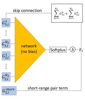
Figure 2: Modifications to the s-NNP form described in Fig. 1 for improving interpretability. The four modifications are: 1) adding skip connections; 2) removing the internal network bias, and adding an external bias, $b$; 3) wrapping the network outputs in a Softplus activation function; and 4) introducing a single short-range pair term using a 2-body filter. The short-range pair term is only allowed to be non-zero up to a cutoff of 2.5 Å.

A central tenet of constructing interpretable models is designing the model architecture in a way that helps isolate the contributions of specific parameter sets to the final model predictions. With this in mind, we therefore propose the five modifications described in Fig. 2. Although the modifications proposed here are only discussed in the context of s-NNP, they can also be applied to many other existing MLIP frameworks.

When applying all of the modifications described in Fig. 2, the full form of s-NNP is written as:

$$E=\sum_{i}E_{i} =\sum_{i}\bigg{[}E_{\text{lin},i}+E_{\text{net},i}\bigg{]}$$ (10)

$$E_{\text{lin},i} =E_{\text{sc},i}+G^{\text{short}}_{2,i}+b$$

$$E_{\text{sc},i} =\sum_{n=1}^{N_{3}}G^{n}_{3,i}+\sum_{n=1}^{N_{2}}G^{n}_{2,i}$$

$$E_{\text{net},i} =\sigma\big{[}N_{\text{no-bias}}(\vec{G}_{i})\big{]},$$

where $E_{\text{sc},i}$ as a “skip connection” term (as used in other DL fields He et al. [2015]), $G^{\text{short}}_{2,i}$ is a short-range 2-body filter, $b$ is a trainable isolated atom energy, $\sigma$ is the Softplus activation function $\sigma(x)=\log{(1+e^{x})}$, and $N_{\text{no-bias}}$ is a neural network with no bias terms on any of its layers. Note that $E_{\text{lin},i}$ encompasses all of the terms which are linearly dependent upon the spline filters, and $E_{\text{net},i}$ captures the non-linear dependence. While a more in-depth discussion of the effects of each of these modifications can be found in Section 4.1, the practical result of Eqn. 10 is that the spline filter visualizations like those shown in Fig. 3 can be intuitively understood. For example, negative regions of the filters will usually correspond to negative $E_{i}$, and positive regions of the filters will always correspond to positive $E_{i}$. While Eqn. 10 still suffers from some drawbacks, predominantly associated with the non-linear effects of $N_{\text{no-bias}}(\vec{G}_{i})$, we believe that it strikes a good balance between the accuracy achieved through a NN architecture, and the interpretability characteristic of classical potentials.

2.3 Benchmarking dataset: Al

In order to test our framework, in Section 3.1 we fit s-NNP models to the aluminum dataset from Smith et al. Smith et al. [2021], which serves as a good benchmarking dataset due to its size and configurational complexity. This dataset was built using an active learning technique for generating interatomic potential training data Smith et al. [2018]. It has also been shown to contain extremely diverse atomic environments, such that the ANI model Smith et al. [2019] which was originally trained to the dataset was tested for use in shock simulations. After removing duplicate calculations (identical atomic positions and computed energies/forces, generated at different active learning steps), and one outlier configuration with particularly high forces, the final dataset consisted of 5,751 unique configurations (744,356 atoms total) with their corresponding DFT-computed energies and forces. A 90:10 train-test split was performed to partition the dataset into training/testing data. This data can be obtained from the original source ani .

2.4 Additional datasets: Cu, Ge, Mo

As a test of the flexibility of the spline filters, in Section 3.3 we trained an s-NNP model simultaneously to the Al dataset described in Section 2.3 and the Cu, Ge, and Mo datasets from Zuo et al. Zuo et al. [2020]. Each dataset from Zuo et al. [2020] was manually constructed and contains the ground state structure for the given element, strained supercells, slab structures, ab initio molecular dynamics (AIMD) sampling of supercells at different temperatures (300 K and $0.5\times$, $0.9\times$, $1.5\times$, and $2.0\times$ the melting point), and AIMD sampling of supercells with single vacancies at 300 K and $2.0\times$ the melting point. On average, each training dataset includes approximately 250 structures for a total of 27,416 atoms (Cu), 14,072 atoms (Ge), and 10,087 atoms (Mo). A detailed summary of the contents of the datasets can be found in Zuo et al. [2020]. This data can be obtained from the original source mle .

In order to attempt to balance the combined dataset, we took a random subset comprised of 20% of the Al dataset in addition to the full Cu, Ge, and Mo datasets, resulting in a total training set size of 1271 Al configurations, 262 Cu, 228 Ge, and 194 Mo. Another logical choice for constructing the multi-element training set would be to further downsample the Al dataset to better balance the relative concentrations of each element type. However, we observed that doing so resulted in worse property predictions for Al, presumably due to the large number of high-energy configurations in the original Al dataset making random sampling of low-energy configurations relevant to the properties of interest unlikely. In all cases, the atomic energies of each element type were shifted by the average energy of that type before training.

3 Results

3.1 Benchmarking tests

Table 1: Fitting results comparing linear s-NNP models, “$(N_{2},N_{3})$ linear”, s-NNP models with neural networks, “$(N_{2},N_{3})$ $l=$*”, s-NNP with interpretability improvements “$(1,8)$ $l=5$, int. *”, and the ANI model from Smith et al. [2021], “ANI”. The $(N_{2},N_{3})$ notation for the spline layers indicates that $N_{2}$ 2-body and $N_{3}$ 3-body spline filters were used. Network architectures are denoted as a tuple of integers (“Network” column) specifying the number of nodes in each hidden layer of the model. Although the training/testing errors decrease significantly when adding additional splines to the linear models, their performance appears to begin to saturate with the “(1,8) linear” model. Model performance only begins to be competitive with the ANI results upon the inclusion of a neural network with sufficient depth, which allows for non-linear combinations of spline outputs. While the “(1,8) $l=5$, int. skip” model only adds the use of skip connections, the “(1,8) $l=5$, int. all” and “(1,8) $l=5$, int. wide” use all of the interpretability improvements discussed in Section 2.2 and Section 4.1. Note that this means that the single 2-body filter specified using the “(1,8)” notation is the short-range pair term described in Fig. 2, and that there are therefore no 2-body filters being passed through the network. Testing errors for the “ANI” model were taken directly from Smith et al. [2021], which did not report training errors. Note that the ANI model uses ensemble-averaging over 8 networks, which they report yields energy and force errors that are “20% and 40% smaller, respectively, compared to a single ANI model”.

Model name	$(N_{2},N_{3})$	Network	Parameters	$E_{\text{RMSE}}$		$F_{\text{RMSE}}$
			(splines, network)	(meV/atom)		(eV/Å)
				Train	Test	Train	Test
$(1,1)$ linear	$(1,1)$	-	(66, 0)	74	78	0.76	0.82
$(1,2)$ linear	$(1,2)$	-	(110, 0)	56	56	0.54	0.58
$(1,4)$ linear	$(1,4)$	-	(198, 0)	40	41	0.46	0.49
$(2,4)$ linear	$(2,4)$	-	(220, 0)	38	36	0.46	0.50
$(1,8)$ linear	$(1,8)$	-	(374, 0)	32	34	0.42	0.46
$(1,2)$ $l=3$	$(1,2)$	$(3,2,1)$	(110, 23)	44	44	0.33	0.35
$(1,4)$ $l=5$	$(1,4)$	$(5,4,3,2,1)$	(198, 80)	10	11	0.22	0.23
$(2,4)$ $l=4$	$(2,4)$	$(6,3,2,1)$	(220, 74)	22	21	0.21	0.21
$(2,4)$ $l=5$	$(2,4)$	$(6,4,3,2,1)$	(220, 96)	8.7	9.0	0.19	0.20
$(2,4)$ $l=6$	$(2,4)$	$(6,5,4,3,2,1)$	(220, 127)	10	12	0.24	0.25
$(1,8)$ $l=5$	$(1,8)$	$(9,8,4,2,1)$	(374, 219)	7.5	6.5	0.13	0.13
$(1,8)$ $l=5$, int. skip	$(1,8)$	$(9,8,4,2,1)$	(374, 219)	5.5	4.6	0.15	0.15
$(1,8)$ $l=5$, int. all	$(1,8)$	$(9,8,4,2,1)$	(374, 219)	5.5	5.9	0.12	0.12
$(1,8)$ $l=5$, int. wide	$(1,8)$	$(128,64,32,16,1)$	(374, 11,793)	5.9	5.1	0.13	0.14
ANI Smith et al. [2021]	-	$(96,96,64,1)$	(-, 15,585)	-	1.9	-	0.06

Using the s-NNP framework, we fit a collection of models to the Al dataset to probe the effects of increasing model capacity in two distinct ways: first by increasing the number of spline filters, and second by increasing the size of the network used for mapping filter outputs to energies. Table 1 outlines the architectures and accuracies of the trained models, grouped by key architectural changes and sorted by total number of parameters. The trained s-NNP models can be conceptually broken down into three main groups, each highlighting the effects of specific architectural changes: 1) “$(N_{2},N_{3})$ linear” models, increasing the number of splines when no neural network is used; 2) “$(N_{2},N_{3})$ $l=$*” models, increasing the number of splines and network size; and 3) introducing the interpretability improvements described in Section 2.2.

The results in Table 1 show multiple avenues for systematically improving the performance of an s-NNP model, though each method appears to experience a saturation point beyond which the model suffers from diminishing returns as complexity increases. Using the “$(1,1)$ linear” model as a baseline, we see that increasing $N_{3}$ from 1 to 8 can monotonically decrease both the energy and the force errors. Increasing $N_{2}$ has no significant effect on the accuracy of the linear models, which is consistent with the notion that a linear combination of cubic Hermite splines can be represented using a single spline.

The introduction of a neural network enables the model to better utilize the additional spline filters, leading to significant improvement of the “$(1,2)$ $l=3$” model over any of the linear models. Increasing the number of spline filters, and subsequently increasing the network width and depth to maintain a “funnel-like” structure (decreasing layer width with increasing depth) can also lead to steady improvements. However, with increasing model size we began to see a commensurate increase in training difficulty, often resulting in larger models with higher errors than what might be expected based on the performance of their smaller counterparts (e.g., “(2,4) $l=6$” compared to “(2,4) $l=5$”, or “(1,8) $l=5$, int. wide” compared to “(1,8) $l=5$, int. all”). Notably, the interpretability improvements from Section 2.2 did not hurt model performance, demonstrating that accuracy and interpretability are not strictly opposing attributes of a model. Based on the results shown in Table 1, we will use the “(1,8) $l=5$, int. all” for all experiments and analyses in the remainder of this paper.

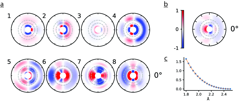
Figure 3: Visualizations of spline filters of the “(1,8) final” model from Table 1 for atomic distances in the range [2.5Å, 7Å]. a) Plots of the individual $G^{\alpha}_{3,i}$ filters, where integer labels above each plot indicate the index $\alpha$. b) The average of all $G^{\alpha}_{3,i}$ 3-body filters. c) The short-range pair term, as described in Section 2.2. Note that the radial splines $f_{c_{j}}^{\alpha}$, $f_{c_{k}}^{\alpha}$, and $\rho_{c_{j}}^{\beta}$ use linear extrapolation for distances outside of the domain defined by their knots. Dashed grey lines in the polar plots correspond to the first and second nearest-neighbor distances (2.86 Å and 4.05 Å respectively) for FCC Al at room temperature Nakashima [2020]. Each point in the polar plots is computed by fixing atom $i$ at the origin, fixing atom $j$ at the given $(r,\theta)$, fixing atom $k$ along the $\theta=0$ axis, then integrating $G^{\alpha}_{3}$ over $r_{k}\in[1.5,7.0]$. Note that there is a forced symmetry in the polar plots since the $g^{\alpha}_{c_{jk}}$ splines in Eqn. 2 take $\cos{(\theta)}$ as input. All polar plots use the same color scale, where values are clipped to fall within a chosen range to optimize for visibility while avoiding information loss. Values for $r<1.5$ Å, which was the smallest distance sampled in the Al dataset as shown in Fig. B1, are omitted to ensure that high signals at small atomic distances would not wash out the rest of the colors in the plots. Though all plots in this figure are technically in units of eV, this would not be true if skip connections were not used.

3.2 Model visualization

A major advantage of s-NNP over many other MLIPs, especially when coupled with the modifications from Section 2.2, is that the spline filters $G_{3,i}^{\alpha}$ and $G_{2,i}^{\beta}$ lend themselves to easy visualization. This can be valuable for helping model developers and users to better understand how their model is interacting with the data or influencing simulation results. The polar plots in Fig. 3a, corresponding to the “(1,8) $l=5$, int. all” model, represent the total activation of the 3-body filters induced by placing an atom at a given $(r,\theta)$. These visualizations make it easy to recognize aspects of the local environments around an atom that are learned during training to have lower energy. For example, the averaged filter shown in Fig. 3b has an attractive behavior of the model for bond angles $60\degree\leq\theta_{jik}\leq 90\degree$ in addition to repulsion for angles larger than approximately $120\degree$. Many of the individual filters in Fig. 3a also show characteristic features at various bond angles, especially for bond lengths near the first and second nearest neighbor distances in FCC aluminum. Fig. 3c shows the short-range pair term, which was learned to have a strongly repulsive contribution, as would be expected based on the Pauli exclusion principle.

It’s worth mentioning that similar plots to the ones shown in Fig. 3 could also be generated for other NNP-like models, for example by visualizing each of the components of the vector output of the first hidden layer in an ANI model. However, most other neural network-based architectures would have significantly more filters to visualize given the size of their hidden layers. For example, the ANI model in Table 1 has 96 nodes in its first hidden layer, thus making it more difficult to interpret the results. Furthermore, since ANI (and most other models) does not use skip connections summing the hidden layer directly into the output, any resultant visualization will not necessarily be in units of energy, meaning it may undergo significant non-linear transformations as it passes through the network.

3.3 Flexibility tests

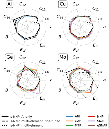
Figure 4: Property predictions of the lattice constant ($a$), cubic elastic constants ($C_{ij}$), bulk modulus ($B$), and vacancy formation and migration energies ($E_{vf}$ and $E_{m}$) for s-NNP models compared to existing MLIPs. s-NNP results are from this work, ANI results from Smith et al. [2021], and all others from Zuo et al. [2020]. All properties have been normalized with respect to the DFT-predicted values. Note that Smith et al. [2021] did not compute $E_{m}$ for ANI. The “(1,8) $l=5$, int. all” model (solid black line), which was trained only to Al, predicts all seven properties well, with the exception of $C_{44}$, which has a relatively small magnitude compared to the other elastic constants. The performance of the multi-element s-NNP model (dashed black lines) is within the range of the other single-element MLIPs, though s-NNP’s predictions for Ge are somewhat distorted. The “fine-tuned” s-NNP model was manually adjusted after training was completed in order improve the property predictions, as described in Section 3.3.

The high interpretablility of the s-NNP spline filters, as discussed in Section 3.2, is particularly valuable when the filters can be applied to different chemical systems in order to enable cross-system comparisons. For example, if multiple s-NNP models using the same spline filters were trained to different chemical systems, then the networks of each model could be analyzed in order to understand how differences in chemistries result in different sensitivities to the local environment embeddings defined by the spline filters. The multi-element model trained to the datasets described in Section 2.4 uses the same spline filters for all of the data, but separate NNs for each element type. The network architecture maintained a funnel-like structure of $(12,8,4,2,1)$. It also used four additional 3-body filters in order to increase its fitting capacity, for a total of one short-range pair filter and 12 3-body filters, though without the use of skip connections or the Softplus activation function. In the case of the multi-element model, the use of skip connections would imply a “background” energy that is consistent across all four element types and is augmented by the network contributions for each element. While this assumption sounds plausible in theory, we found that in practice a model using skip connections resulted in poorer property predictions than one which did not. This decreased performance when using skip connections can likely be attributed to the larger concentration of Al data dominating the fitting and causing the filters to learn a background energy that is influenced by the high-energy Al configurations and therefore not transferable to the lower energy Cu/Ge/Mo data. We believe that further research into constructing balanced training datasets could help address this issue, though it may also be possible that a larger number of splines is required for describing this more diverse dataset. Another alternative, which was not explored here, would be to only use skip connections for a subset of the spline filters in order to give the model the ability to learn a transferable background energy without enforcing the full constraint of skip connections for all filters.

The property predictions of the multi-element model plotted in Fig. 4 show that a model using shared filters for multiple datasets can learn to make reasonable property predictions for all four elements studied in this work. While the initial predictions for most of the elements were relatively good, the cubic elastic constants and bulk modulus for Mo were noticeably under-predicted, and the vacancy migration energy was far too large to be considered acceptable (dotted line in Fig. 4). Due to the relatively few number of spline filters used, and their high degree of interpretablity, we were able to fine-tune the model by zeroing out the network weights of hand-chosen filters in order to remove their contribution to the Mo energy predictions. For example, the contributions of each spline filter can be visualized individually in order to isolate the influence of each filter on the properties of interest (see Fig. C2). Following this approach, we were able to improve the Mo predictions to bring them within an acceptable range without altering the predictions for the other three elements (dashed lines in Fig. 4). However, we note that the original training errors of the model (before fine-tuning) as shown in Fig. C4 were comparable to those of the NNIPs from Zuo et al. [2020], suggesting that the property predictions of the multi-element s-NNP model may have been able to have been improved by re-balancing the dataset. Similar to what was described in Section 2.4, a possible explanation for this is that the Mo dataset did not fully constrain the portions of the spline filters relevant to computing the properties of interest, and their shapes were therefore dictated by the Al dataset, leading to corrupted Mo property predictions. Further research into methods for preventing this type of “cross-pollution” of information would be valuable for constructing more flexible and generalizable models.

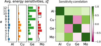
Figure 5: Analysis of sensitivities $s^{\alpha}_{E}$ (Eqn. 11) of the predicted energies with respect to the 3-body spline filters, $G^{\alpha}_{3}$, for each elemental model. We compute the sensitivity by calculating the derivative of the predicted energy with respect to the spline filter outputs, normalized by the DFT reference value, then summing over all atoms in the training set. Note that these sensitivities are computed with respect to the total energy $E$, which includes the network contributions. The left panel plots the raw values, while the right panel shows the correlation between the sensitivities of each element. The empty bars for Mo correspond to the filters which were removed from the Mo energy predictions during fine-tuning as described in Section 3.3. The corresponding spline filters are visualized in Fig. C1.

In order to gain additional insights into the differences in energetics between the Al, Cu, Ge, and Mo systems, we compute the sensitivities of the energies predicted by the multi-element model with respect to each of the 3-body spline filters. The sensitivity of the total energy, $E$, for all configurations $N$ with respect to a given 3-body spline filter $G^{\alpha}_{3}$ can be computed as:

$$s^{\,\alpha}_{E}=\sum_{i=1}^{N}|\partial E_{\text{s-NNP}}/\partial G_{3,i}^{\alpha}|/E_{\text{DFT}},$$ (11)

which can be easily computed via back-propagation.

Calculation and comparison of these sensitivities for each dataset, as shown in Fig. 5, highlight the learned similarities and differences between the four elemental datasets. Examination of the correlation between the sensitivities (right panel of Fig. 5) shows that the Cu and Mo datasets have similar filter sensitivities, while Ge is the only element to have a negative correlation with any of the other elements. The Al dataset appears to be uniformly similar to all three remaining elements, reflecting the fact that most of the geometric configurations of the Cu/Ge/Mo datasets are well-sampled by the Al dataset (see Fig. C3). We hypothesize that the negative correlation of the Ge sensitivities is due to an attempt by the model to encode the large cluster of outlying Ge points in the UMAP visualizations shown in Fig. C3.

4 Discussion

4.1 Understanding model behavior

The main purpose behind the modifications proposed in Fig. 2 and Section 2.2 is to simplify the process of understanding the behavior of s-NNP models. This not only improves the usefulness of visualizations like those shown in Fig. 3 and Fig. C1, but can also aid in debugging model predictions in practice. In this section, we will discuss each modification from Section 2.2 in greater detail in order to highlight how they improve the interpretability of the model.

The first of these modifications is the use of skip connections, which result in strong theoretical changes that can not only lead to improved trainability as seen in Table 1 and other deep learning applications Li et al. [2017], but also greatly increase the interpretability of the model. Modifying $\vec{G}_{i}$ to have units of energy seemingly contrasts with the notion of the atomic “density”, $n_{i}$, from Eqn. 1 and the local environment descriptor, $\vec{D}_{i}$, from Eqn. 4, both of which are considered to be intermediate representations which will only become energies once they have been transformed by a regression function ($U_{c_{i}}$ or $N_{c_{i}}$ respectively). However, we emphasize that these three quantities ($n_{i}$, $\vec{D}_{i}$, and $\vec{G}_{i}$) remain closely related even when $\vec{G}_{i}$ is in units of energy while the others are not. Although local environment descriptors are usually seen as quantifying the geometry within a local neighborhood, there is no reason that the environment descriptor may not itself also be an energy. An energy-based descriptor could then be thought of as a type of energy partitioning scheme, where in the case of s-NNP with skip connections the atomic energies contribute both linearly to the total energy (through the skip connection) and non-linearly (through the network). In fact, in our previous work Vita and Trinkle [2021] we observed that $U_{c_{i}}$ was often learned to be a nearly linear function, meaning that it essentially served the purpose of a simple unit conversion for $n_{i}$. This linearity is essential to model interpretability, and is the main motivator for the use of skip connections in s-NNP, as it is a step towards simplifying the process of understanding how the spline filters contribute to the total energy.

Nevertheless, care must still be taken when interpreting the filter visualizations when the other modifications discussed in Section 2.2 are not also employed. For example, skip connections alone do not guarantee that a negative filter value means $E_{i}$ will also be negative, since the network contribution $N(\vec{G}_{i})$ may outweigh the skip connection term. Similarly, adjusting the filter outputs (e.g., by tuning the knot positions) may have unexpected results due to the non-linear behavior of the network. These issues are also present with all non energy-based descriptors like $n_{i}$ and $\vec{D}_{i}$, but can be further improved upon using the remaining techniques discussed in this section.

In order to further facilitate straightforward interpretation of spline visualizations, we also choose to pin the knots of the radial splines to be 0 at the cutoff distance $r_{c}$, and we remove bias terms from the layers of the NN. As a result of this, both $N(\vec{G}_{i})$ and $E_{\text{sc},i}$ will smoothly decay to 0 at the cutoff distance, thus incorporating the desired behavior which is enforced in the Behler-Parrinello NNP using the cutoff function $v_{c}$ in Eqn. 6. In order to account for the fact that some datasets may have non-zero energy at the cutoff distance, an external bias term, $b$ is added so that the atomic energy converges to $b$ at $r_{c}$. In this sense, $b$ corresponds to the learned energy of the isolated atom. We note that this external bias term is preferable to using internal network bias or un-pinning the radial splines because it ensures that $N(\vec{G}_{i})$ and $E_{\text{sc},i}$ behave similarly as $r_{ij}$ approaches $r_{c}$.

Wrapping the network output $N_{\text{no-bias}}(\vec{G}_{i})$ in the Softplus activation function guarantees that the NN contributions to the total energy are strictly non-negative. This ensures that any attractive behavior of the model arises solely from the spline filters through the skip connection term, $E_{\text{sc},i}$, thus helping to isolate certain model behaviors to specific parameter sets. It is important to note, however, that the Softplus activation should only be used in conjunction with skip connections in order to ensure that the model can predict negative energies.

A common challenge for many MLIPs is ensuring a repulsive behavior at small values of $r_{ij}$. This difficulty is not reflected in classical potentials, however, as classical models often include explicit repulsive terms. While a data-driven solution to this problem is possible, by explicitly adding short-range dimers into the training dataset, many MLIP developers choose instead to adjust the form of their IP. One such method used in the literature is to augment the model by introducing an auxiliary potential designed to capture the repulsive behavior of a pair potential. For example, in Milardovich et al. [2023] a “composite potential” was constructed by first fitting a repulsive “auxiliary potential” to DFT data, then fitting a “main potential” to the residuals of the pair potential using a Gaussian Approximation Potential Bartók et al. [2010]. We incorporate a similar idea by including a short-range 2-body filter, $G_{2,i}$, which is summed directly into the total energy without ever passing through the NN. Note that this is different from the skip connections, which are summed directly into the energy and passed through the NN. Having a spline filter which only contributes linearly to the total energy means that it is free of any of the interpretability issues described for the spline filters which are used as input to the NN. While this short-range pair term does not necessarily guarantee a repulsive behavior at small distances, we observe empirically that it is often learned during training to have a strongly repulsive shape. A similar technique is used by the SNAP interatomic potential Wood and Thompson [2018], where the repulsive ZBL pair potential is added to the potential form as a “reference potential”.

4.2 s-NNP’s relation to other models

The s-NNP architecture shown in Fig. 1 can be further understood by drawing relationships between itself and other models from the literature, particularly the UF3 model Xie et al. [2021] and the original Behler-Parrinello NNP Behler and Parrinello [2007]. s-NNP can be compared to UF3 and NNP by analyzing the differences between the two key components of each model: the embedding function for encoding local atomic environments into a descriptor, and the regression function for mapping the descriptor into an energy. Although it can be difficult to clearly distinguish between the embedding/regression portions of most MLIPs due to the inability to definitively establish the roles of all parameters in a deep model, we will attempt to break each model down in intuitive ways to facilitate comparison. One can view the vector $\vec{G}_{i}$ from Eqn. 9 as a descriptor generated by an embedding function defined by the spline filters $G^{\alpha}_{3,i}$ and $G^{\beta}_{2,i}$. This embedding technique is most similar to the UF3 method, which also decomposes the energy into two-body and three-body terms described by spline basis functions. Though there are some differences in the exact details of the UF3 and s-NNP spline functions, for example UF3’s use of tricubic B-splines instead of the 1D cubic Hermite splines of s-NNP, the general principle is the same. While s-NNP’s embedding function is most similar to that of UF3, its regression function is identical to that of the Behler-Parrinello NNP Behler and Parrinello [2007]. Therefore, in order to help analyze the performance of s-NNP with respect to other models in the literature, it is suitable to think of s-NNP as a combination of a UF3-like embedding function with an NNP regressor. Or, equivalently, as an NNP using a spline-based embedding function instead of atom-centered symmetry functions Behler and Parrinello [2007]. However, neither UF3 nor NNP utilize all of the interpretability improvements discussed in Section 2.2.

The recently-proposed EAM-R model Nitol et al. [2023] is the most closely related model to s-NNP in the literature, as it also incorporates components of both a classical model (EAM) and an MLIP (an NNP). EAM-R is a composite potential (using the terminology described in Section 4.1) where the auxiliary potential is an EAM model, and the main potential is an RANN (an NNP with descriptors inspired by the analytical MEAM equations Baskes [1992]). Similar to this work, the developers of EAM-R observed that combining a classical model with an MLIP resulted in both improved stability relative to an MLIP and improved accuracy to a classical potential alone. Despite s-NNP’s similarity to EAM-R, s-NNP has some key differences, namely the use of spline filters (instead of analytical MEAM-inspired descriptors) and some of the interpretability improvements discussed in Section 2.2. In particular, the spline filters may be expected to be more flexible than the RANN descriptors (similar to how s-MEAM is more flexible than analytical MEAM) for a given computational cost, and benefit from the ability to enforce smoothness and convergence through curvature penalties and knot pinning. Furthermore, s-NNP’s use of skip connections and the removal of the internal network bias greatly improve the interpretablily of the model, as discussed in Section 2.2. Although EAM-R does not include these modifications, it is an excellent example of an MLIP which could easily incorporate these same interpretability improvements.

4.3 Computational costs

The computational cost of s-NNP is dominated by the evaluation of $\vec{G}_{i}$, and is particularly dependant upon the choice of $N_{3}$. In fact, basic profiling tests revealed that the filter evaluations accounted for approximately 95% of the total CPU and GPU time. This behavior can be understood heuristically by the fact that Eqn. 2 involves approximately $\mathcal{O}(N_{n}^{2})$ spline evaluations for each filter where $N_{n}$ is the average number of neighbors within the cutoff distance (due to the summation over triplets of atoms), as opposed to the relatively few matrix multiplications associated with the evaluation of the neural network. In general, the computational cost of inference with an s-NNP potential will scale sub-linearly with $N_{3}$ (some speedup can be achieved by performing batched spline evaluations for the filters in Eqn. 2). An important practical implication of this is that in order to improve the accuracy of a given s-NNP model (and other NNP-based MLIPs as well), it is much more computationally efficient to increase the size of the network rather than the size of the embedding function. On the other hand, increasing $N_{3}$ may lead to larger increases in accuracy (up to a point) than what is achievable by only increasing the network size

Given the performances of the s-NNP models in Table 1 and the timing comparisons observed in our previous work between s-MEAM and a NNP Vita and Trinkle [2021], it may be expected that an s-NNP could be constructed that achieves identical errors to ANI while maintaining a higher speed. The “(1,8) $l=5$, int. all” model is already nearing this threshold, especially taking into account that the values for ANI reported in Table 1 use ensemble-averages over 8 models, as reported by the original authors Smith et al. [2021], which they say can make the energy and force errors “20% and 40% smaller, respectively” and may account for the differences in performance as compared to “(1,8) $l=5$, int. all”.

5 Conclusion

In this work we developed a novel framework using spline-based filters coupled with a neural network regressor in order to blend the strengths of both classical and ML IPs. We use this framework to probe the gap between these two classes of models, observing performance limits of linear (“classical”) models that can be overcome using even small neural networks. We then show that this improved performance can be maintained while incorporating architectural changes which improve the interpretability of the model, such as the use of skip connections, an external bias term, a Softplus activation function, and a short-range pair term. Finally, we demonstrate that the information-rich filter layer can be used as a reference point for performing cross-system analyses, and correlate well enough with model behavior to enable manual tuning to improve property predictions. Future studies applying the visualization techniques shown here to practical applications, and exploring methods of isolating contributions of specific elements to subsets of the model parameters would be valuable for continuing to refine the interpretability improvements explored in this work. Furthermore, efforts building upon this work could continue to improve the s-NNP design by incorporating equivariance or a message-passing network, which may lead to better performance and improved scaling of model size with number of elements.

6 Code and Data Availability

The code used for training s-NNP models can be found at https://github.com/TrinkleGroup/snnp. All datasets can be obtained from their original sources.

7 Acknowledgements

This research was supported by the National Science Foundation through awards NSF/NRT-1922758 and NSF/HDR-1940303. Computational resources were provided on the HAL computing cluster Kindratenko et al. [2020] by the National Center for Supercomputing Applications.

Appendix A Training details

All s-NNP models in this work were trained using the code provided at https://github.com/TrinkleGroup/snnp on a single GPU from the HAL computing cluster Kindratenko et al. [2020]. The energy and force terms in the loss function were given weights of 10 and 1 respectively. L2 regularization was applied to the network parameters with a weight of 0.01. The AMSGrad variant of the Adam optimizer was used, with an initial learning rate of 0.001 and a MultiStepLR scheduler. Inner and outer cutoff radii of 2.5 and 7.0 were used, as specified in the main text.

Appendix B Distributions of $r_{ij}$ and $\theta_{jik}$

Fig. B1 shows that the Al dataset well samples the range of $r_{ij}$ and $\cos{\theta_{jik}}$ values present in the Cu, Ge, and Mo datasets. Notably, the Al dataset has a much more uniform sampling of both of these values, likely due to both its large size and more diverse sampling technique (active learning). These results suggest that the Al dataset may help to constrain regions of the 2-body and 3-body splines that are under-sampled by the other three datasets. The inner cutoff radius of 2.5 $\AA$ (below which the short-range pair term becomes non-zero) was chosen to be slightly larger than the smallest atomic distances sampled by the datasets in order to ensure that the inner knots of the splines would be well constrained by the data.

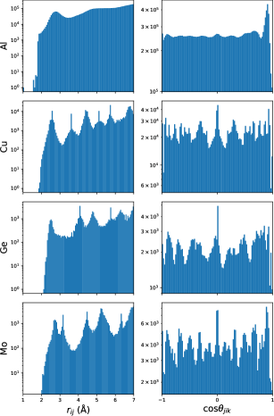
Figure B1: Histograms of $r_{ij}$ and $\cos{\theta_{jik}}$ values sampled from the Al, Cu, Ge, and Mo datasets used in this work.

Appendix C Multi-element model

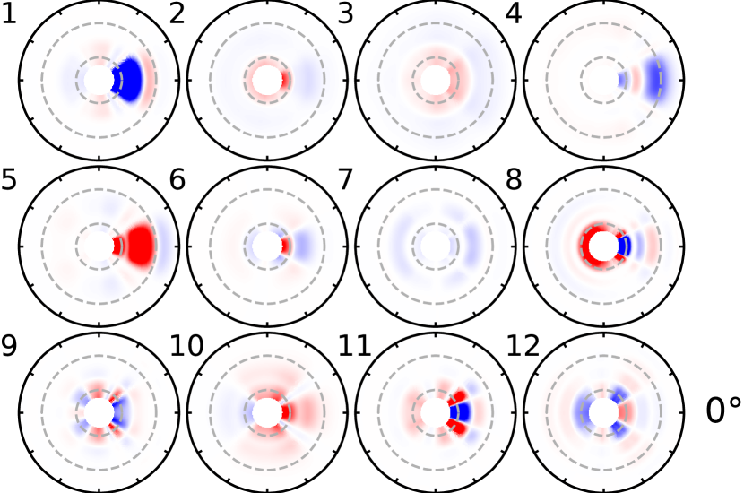
Figure C1: Polar plot visualizations of the 3-body spline filters for the multi-element s-NNP. Grey dashed lines mark 2Å and 5Å for reference.

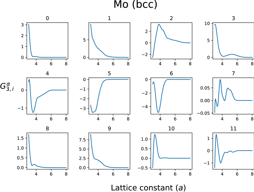
Figure C2: Spline filter activations, $G_{3,i}^{\alpha}$, for the multi-element model from Section 3.3 on the $E$ vs. $a$ curve for BCC Mo. Filter numbers 1 and 9 were removed from the Mo property predictions during the fine-tuning process by zeroing out the corresponding network weights as described in Section 3.3.

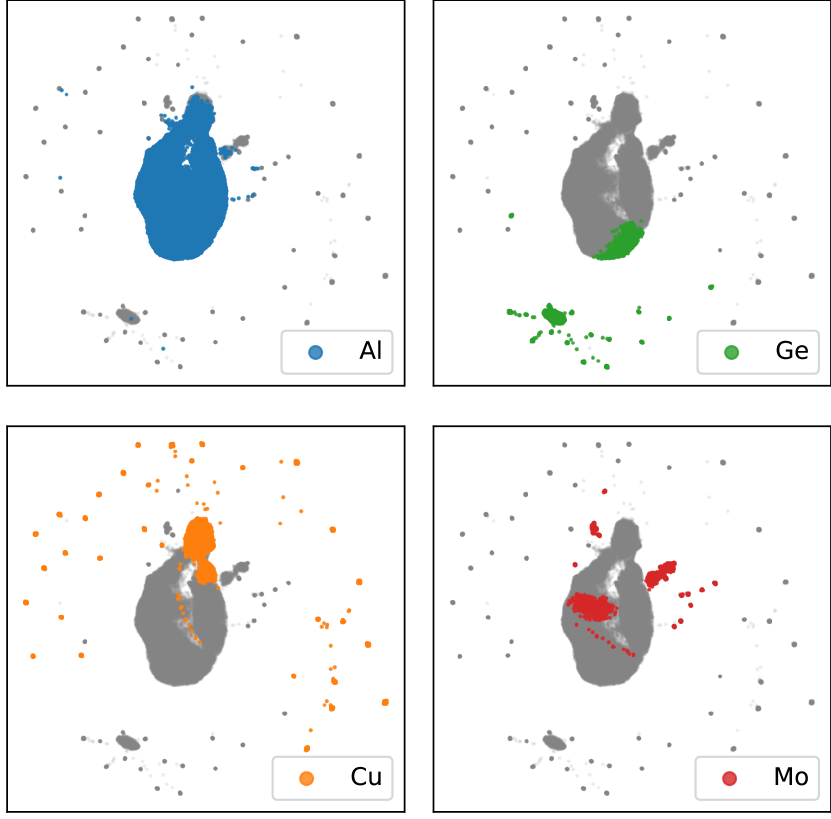
Figure C3: UMAP plots of the vectors $\vec{G_{i}}$ generated by applying the spline filters from the multi-element s-NNP model from Section 3.3, colored by element type.

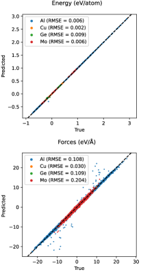
Figure C4: Parity plots for energy and force predictions of the multi-element model described in Section 3.3 before manual fine-tuning of the model. The computed RMSE values match the expected errors for NN-based MLIPs on the Cu/Ge/Mo dataset based on the results from Zuo et al. [2020], though the s-NNP model here uses a larger cutoff distance. Note that the RMSE value for Al should not be compared directly to those in Table 1, since the results here use only the 20% of the Al dataset as described in Section 2.4.

Fig. C1 shows the spline filter visualizations corresponding to the 12 splines used by the multi-element model. As described in Section 3.3, the multi-element model does not use skip connections, which means that the filters in Fig. C1 are not necessarily in units of energy and may be drastically transformed before being mapped into the output of the model. Although this greatly reduces the utility of the spline visualizations, the filters can still be understood in the context of the model sensitivities reported in Fig. 5. It can be seen that filters 1 and 9 (which were removed during the manual fine-tuning process) both have negative activations for short bond lengths and bond angles less than $30\degree$. The filters can be further analyzed by plotting their activations over a range of lattice constants, as shown in Fig. C2, which reveals that filters 1 and 9 both yield strongly repulsive contributions for small lattice constants. The removal of these filters for the Mo predictions drastically lowered the predicted $E_{m}$, which is consistent with our intuition that removal of filters 1 and 9 should result in a softer potential.

Fig. C3 supports the expectation from Section B that the Al dataset encompasses a majority of the data from the Cu/Ge/Mo datasets. As can be seen from Fig. C3, this statement appears to be generally true, with the exceptions of some small outlying clusters of Cu and Ge points. The small isolated clusters surrounding the main manifold correspond to the strained configurations from the Cu/Ge/Mo datasets, while the larger outlying cluster of Ge points correspond to a subset of the Ge configurations which were sampled by low- and high-temperature MD simulations.

Fig. C4 provides a breakdown of the errors of the multi-element model (prior to fine-tuning) for each elemental datasets. The apparent contradiction between the low RMSE values (compared to those from Zuo et al. [2020]) shown in Fig. C4 and the unacceptably high errors in property predictions for Mo reported in Fig. 4 suggests that the configurations in the Mo dataset were not sufficiently representative of the properties of interest. While it is possible that the property predictions of the multi-element s-NNP may have been able to be improved if even lower Mo RMSE values could have been obtained, the fact that many models with similar errors (Zuo et al. [2020] and Vita and Trinkle [2021]) had good property predictions suggests some kind of deficiency in the dataset which would require further analysis in order understand fully.

References

- Behler and Parrinello [2007] Jörg Behler and Michele Parrinello. Generalized neural-network representation of high-dimensional potential-energy surfaces. Physical Review Letters, 98(14), April 2007. doi: 10.1103/physrevlett.98.146401.
- Bartók et al. [2010] Albert P. Bartók, Mike C. Payne, Risi Kondor, and Gábor Csányi. Gaussian approximation potentials: The accuracy of quantum mechanics, without the electrons. Phys. Rev. Lett., 104:136403, Apr 2010. doi: 10.1103/PhysRevLett.104.136403.
- Batzner et al. [2022] Simon Batzner, Albert Musaelian, Lixin Sun, Mario Geiger, Jonathan P. Mailoa, Mordechai Kornbluth, Nicola Molinari, Tess E. Smidt, and Boris Kozinsky. E(3)-equivariant graph neural networks for data-efficient and accurate interatomic potentials. Nature Communications, 13(1):2453, 2022. ISSN 2041-1723. doi: 10.1038/s41467-022-29939-5. URL https://www.nature.com/articles/s41467-022-29939-5.
- Thompson et al. [2015] A.P. Thompson, L.P. Swiler, C.R. Trott, S.M. Foiles, and G.J. Tucker. Spectral neighbor analysis method for automated generation of quantum-accurate interatomic potentials. Journal of Computational Physics, 285:316–330, March 2015. doi: 10.1016/j.jcp.2014.12.018.
- Shapeev [2016] Alexander V. Shapeev. Moment tensor potentials: A class of systematically improvable interatomic potentials. Multiscale Modeling & Simulation, 14(3):1153–1173, January 2016. doi: 10.1137/15m1054183.
- Drautz [2019] Ralf Drautz. Atomic cluster expansion for accurate and transferable interatomic potentials. Physical Review B, 99(1), January 2019. doi: 10.1103/physrevb.99.014104. URL https://doi.org/10.1103/physrevb.99.014104.
- Gilmer et al. [2017] Justin Gilmer, Samuel S. Schoenholz, Patrick F. Riley, Oriol Vinyals, and George E. Dahl. Neural Message Passing for Quantum Chemistry. arXiv:1704.01212, 2017. URL http://arxiv.org/abs/1704.01212.
- Schütt et al. [2018] K. T. Schütt, H. E. Sauceda, P.-J. Kindermans, A. Tkatchenko, and K.-R. Müller. SchNet – A deep learning architecture for molecules and materials. The Journal of Chemical Physics, 148(24):241722, 2018. ISSN 0021-9606. doi: 10.1063/1.5019779. URL http://aip.scitation.org/doi/10.1063/1.5019779.
- Batatia et al. [2022a] Ilyes Batatia, Simon Batzner, Dávid Péter Kovács, Albert Musaelian, Gregor N. C. Simm, Ralf Drautz, Christoph Ortner, Boris Kozinsky, and Gábor Csányi. The Design Space of E(3)-Equivariant Atom-Centered Interatomic Potentials. arXiv, may 2022a. URL http://arxiv.org/abs/2205.06643.
- Mueller et al. [2020] Tim Mueller, Alberto Hernandez, and Chuhong Wang. Machine learning for interatomic potential models. The Journal of Chemical Physics, 152(5):050902, 2020. ISSN 0021-9606. doi: 10.1063/1.5126336. URL http://aip.scitation.org/doi/10.1063/1.5126336.
- Manzhos and Carrington [2021] Sergei Manzhos and Tucker Carrington. Neural Network Potential Energy Surfaces for Small Molecules and Reactions. Chemical Reviews, 121(16):10187–10217, 2021. ISSN 0009-2665. doi: 10.1021/acs.chemrev.0c00665. URL https://doi.org/10.1021/acs.chemrev.0c00665https://pubs.acs.org/doi/10.1021/acs.chemrev.0c00665.
- Christensen et al. [2020] Anders S. Christensen, Lars A. Bratholm, Felix A. Faber, and O. Anatole von Lilienfeld. FCHL revisited: Faster and more accurate quantum machine learning. The Journal of Chemical Physics, 152(4):044107, 2020. ISSN 0021-9606. doi: 10.1063/1.5126701. URL http://aip.scitation.org/doi/10.1063/1.5126701.
- Musaelian et al. [2022] Albert Musaelian, Simon Batzner, Anders Johansson, Lixin Sun, Cameron J. Owen, Mordechai Kornbluth, and Boris Kozinsky. Learning Local Equivariant Representations for Large-Scale Atomistic Dynamics. arXiv:2204.05249, 2022. URL http://arxiv.org/abs/2204.05249.
- Gasteiger et al. [2021] Johannes Gasteiger, Florian Becker, and Stephan Günnemann. GemNet: Universal Directional Graph Neural Networks for Molecules. arXiv:2106.08903, 2021. URL http://arxiv.org/abs/2106.08903.
- Haghighatlari et al. [2021] Mojtaba Haghighatlari, Jie Li, Xingyi Guan, Oufan Zhang, Akshaya Das, Christopher J. Stein, Farnaz Heidar-Zadeh, Meili Liu, Martin Head-Gordon, Luke Bertels, Hongxia Hao, Itai Leven, and Teresa Head-Gordon. NewtonNet: A Newtonian message passing network for deep learning of interatomic potentials and forces. arXiv:2108.02913, 2021. URL http://arxiv.org/abs/2108.02913.
- Lubbers et al. [2018] Nicholas Lubbers, Justin S. Smith, and Kipton Barros. Hierarchical modeling of molecular energies using a deep neural network. The Journal of Chemical Physics, 148(24):241715, 2018. ISSN 0021-9606. doi: 10.1063/1.5011181. URL http://aip.scitation.org/doi/10.1063/1.5011181.
- Hu et al. [2021] Weihua Hu, Muhammed Shuaibi, Abhishek Das, Siddharth Goyal, Anuroop Sriram, Jure Leskovec, Devi Parikh, and C Lawrence Zitnick. ForceNet: A graph neural network for large-scale quantum calculations. arXiv:2103.01436, 2021.
- Batatia et al. [2022b] Ilyes Batatia, Simon Batzner, Dávid Péter Kovács, Albert Musaelian, Gregor N. C. Simm, Ralf Drautz, Christoph Ortner, Boris Kozinsky, and Gábor Csányi. The Design Space of E(3)-Equivariant Atom-Centered Interatomic Potentials. arXiv:2205.06643, 2022b. URL http://arxiv.org/abs/2205.06643.
- Sosso et al. [2016] Gabriele C. Sosso, Ji Chen, Stephen J. Cox, Martin Fitzner, Philipp Pedevilla, Andrea Zen, and Angelos Michaelides. Crystal nucleation in liquids: Open questions and future challenges in molecular dynamics simulations. Chemical Reviews, 116(12):7078–7116, May 2016. doi: 10.1021/acs.chemrev.5b00744. URL https://doi.org/10.1021/acs.chemrev.5b00744.
- Ravelo et al. [2013] R. Ravelo, T. C. Germann, O. Guerrero, Q. An, and B. L. Holian. Shock-induced plasticity in tantalum single crystals: Interatomic potentials and large-scale molecular-dynamics simulations. Physical Review B, 88(13), October 2013. doi: 10.1103/physrevb.88.134101. URL https://doi.org/10.1103/physrevb.88.134101.
- Diemand et al. [2013] Jürg Diemand, Raymond Angélil, Kyoko K. Tanaka, and Hidekazu Tanaka. Large scale molecular dynamics simulations of homogeneous nucleation. The Journal of Chemical Physics, 139(7):074309, August 2013. doi: 10.1063/1.4818639. URL https://doi.org/10.1063/1.4818639.
- Phillips et al. [2020] James C. Phillips, David J. Hardy, Julio D. C. Maia, John E. Stone, João V. Ribeiro, Rafael C. Bernardi, Ronak Buch, Giacomo Fiorin, Jérôme Hénin, Wei Jiang, Ryan McGreevy, Marcelo C. R. Melo, Brian K. Radak, Robert D. Skeel, Abhishek Singharoy, Yi Wang, Benoît Roux, Aleksei Aksimentiev, Zaida Luthey-Schulten, Laxmikant V. Kalé, Klaus Schulten, Christophe Chipot, and Emad Tajkhorshid. Scalable molecular dynamics on CPU and GPU architectures with NAMD. The Journal of Chemical Physics, 153(4):044130, July 2020. doi: 10.1063/5.0014475. URL https://doi.org/10.1063/5.0014475.
- Zepeda-Ruiz et al. [2017] Luis A. Zepeda-Ruiz, Alexander Stukowski, Tomas Oppelstrup, and Vasily V. Bulatov. Probing the limits of metal plasticity with molecular dynamics simulations. Nature, 550(7677):492–495, September 2017. doi: 10.1038/nature23472. URL https://doi.org/10.1038/nature23472.
- Jones [1924] J. E. Jones. On the determination of molecular fields. —II. from the equation of state of a gas. Proceedings of the Royal Society of London. Series A, Containing Papers of a Mathematical and Physical Character, 106(738):463–477, October 1924. doi: 10.1098/rspa.1924.0082.
- Daw and Baskes [1984] Murray S. Daw and M. I. Baskes. Embedded-atom method: Derivation and application to impurities, surfaces, and other defects in metals. Physical Review B, 29(12):6443–6453, June 1984. doi: 10.1103/physrevb.29.6443.
- Buckingham [1938] R. A. Buckingham. The classical equation of state of gaseous helium, neon and argon. Proceedings of the Royal Society of London. Series A. Mathematical and Physical Sciences, 168(933):264–283, October 1938. doi: 10.1098/rspa.1938.0173.
- Tersoff [1986] J. Tersoff. New empirical model for the structural properties of silicon. Physical Review Letters, 56(6):632–635, February 1986. doi: 10.1103/physrevlett.56.632.
- Brenner et al. [2002] Donald W Brenner, Olga A Shenderova, Judith A Harrison, Steven J Stuart, Boris Ni, and Susan B Sinnott. A second-generation reactive empirical bond order (REBO) potential energy expression for hydrocarbons. Journal of Physics: Condensed Matter, 14(4):783–802, January 2002. doi: 10.1088/0953-8984/14/4/312.
- Shan et al. [2010] Tzu-Ray Shan, Bryce D. Devine, Travis W. Kemper, Susan B. Sinnott, and Simon R. Phillpot. Charge-optimized many-body potential for the hafnium/hafnium oxide system. Physical Review B, 81(12), March 2010. doi: 10.1103/physrevb.81.125328.
- van Duin et al. [2001] Adri C. T. van Duin, Siddharth Dasgupta, Francois Lorant, and William A. Goddard. ReaxFF: a reactive force field for hydrocarbons. The Journal of Physical Chemistry A, 105(41):9396–9409, October 2001. doi: 10.1021/jp004368u. URL https://doi.org/10.1021/jp004368u.
- Baskes [1992] M. I. Baskes. Modified embedded-atom potentials for cubic materials and impurities. Physical Review B, 46(5):2727–2742, August 1992. doi: 10.1103/physrevb.46.2727.
- Lenosky et al. [2000] T. J. Lenosky, B. Sadigh, E. Alonso, V. V. Bulatov, T. D. de la Rubia, J. Kim, A. F. Voter, and J. D. Kress. Highly optimized empirical potential model of silicon. Modelling and Simulation in Materials Science and Engineering, 8(6):825–841, October 2000. doi: 10.1088/0965-0393/8/6/305.
- Hornik et al. [1989] Kurt Hornik, Maxwell Stinchcombe, and Halbert White. Multilayer feedforward networks are universal approximators. Neural Networks, 2(5):359–366, January 1989. doi: 10.1016/0893-6080(89)90020-8. URL https://doi.org/10.1016/0893-6080(89)90020-8.
- Smith et al. [2017] J. S. Smith, O. Isayev, and A. E. Roitberg. ANI-1: an extensible neural network potential with DFT accuracy at force field computational cost. Chemical Science, 8(4):3192–3203, 2017. doi: 10.1039/c6sc05720a. URL https://doi.org/10.1039/c6sc05720a.
- Stillinger and Weber [1985] Frank H. Stillinger and Thomas A. Weber. Computer simulation of local order in condensed phases of silicon. Physical Review B, 31(8):5262–5271, April 1985. doi: 10.1103/physrevb.31.5262.
- He et al. [2015] Kaiming He, Xiangyu Zhang, Shaoqing Ren, and Jian Sun. Deep residual learning for image recognition, 2015. URL https://arxiv.org/abs/1512.03385.
- Smith et al. [2021] Justin S. Smith, Benjamin Nebgen, Nithin Mathew, Jie Chen, Nicholas Lubbers, Leonid Burakovsky, Sergei Tretiak, Hai Ah Nam, Timothy Germann, Saryu Fensin, and Kipton Barros. Automated discovery of a robust interatomic potential for aluminum. Nature Communications, 12(1), February 2021. doi: 10.1038/s41467-021-21376-0. URL https://doi.org/10.1038/s41467-021-21376-0.
- Smith et al. [2018] Justin S. Smith, Ben Nebgen, Nicholas Lubbers, Olexandr Isayev, and Adrian E. Roitberg. Less is more: Sampling chemical space with active learning. The Journal of Chemical Physics, 148(24):241733, June 2018. doi: 10.1063/1.5023802. URL https://doi.org/10.1063/1.5023802.
- Smith et al. [2019] Justin S. Smith, Benjamin T. Nebgen, Roman Zubatyuk, Nicholas Lubbers, Christian Devereux, Kipton Barros, Sergei Tretiak, Olexandr Isayev, and Adrian E. Roitberg. Approaching coupled cluster accuracy with a general-purpose neural network potential through transfer learning. Nature Communications, 10(1), July 2019. doi: 10.1038/s41467-019-10827-4. URL https://doi.org/10.1038/s41467-019-10827-4.
- [40] atomistic-ml/ani-al repository. https://github.com/atomistic-ml/ani-al. Accessed: 2010-09-30.
- Zuo et al. [2020] Yunxing Zuo, Chi Chen, Xiangguo Li, Zhi Deng, Yiming Chen, Jörg Behler, Gábor Csányi, Alexander V. Shapeev, Aidan P. Thompson, Mitchell A. Wood, and Shyue Ping Ong. Performance and cost assessment of machine learning interatomic potentials. The Journal of Physical Chemistry A, 124(4):731–745, January 2020. doi: 10.1021/acs.jpca.9b08723. URL https://doi.org/10.1021/acs.jpca.9b08723.
- [42] materialsvirtuallab/mlearn repository. https://github.com/materialsvirtuallab/mlearn. Accessed: 2010-09-30.
- Nakashima [2020] Philip N. H. Nakashima. The crystallography of aluminum and its alloys. 2020. doi: 10.48550/ARXIV.2002.01562. URL https://arxiv.org/abs/2002.01562.
- Li et al. [2017] Hao Li, Zheng Xu, Gavin Taylor, Christoph Studer, and Tom Goldstein. Visualizing the loss landscape of neural nets, 2017. URL https://arxiv.org/abs/1712.09913.
- Vita and Trinkle [2021] Joshua A. Vita and Dallas R. Trinkle. Exploring the necessary complexity of interatomic potentials. Computational Materials Science, 200:110752, December 2021. doi: 10.1016/j.commatsci.2021.110752. URL https://doi.org/10.1016/j.commatsci.2021.110752.
- Milardovich et al. [2023] Diego Milardovich, Dominic Waldhoer, Markus Jech, Al-Moatasem Bellah El-Sayed, and Tibor Grasser. Building robust machine learning force fields by composite gaussian approximation potentials. Solid-State Electronics, 200:108529, February 2023. doi: 10.1016/j.sse.2022.108529. URL https://doi.org/10.1016/j.sse.2022.108529.
- Wood and Thompson [2018] Mitchell A. Wood and Aidan P. Thompson. Extending the accuracy of the SNAP interatomic potential form. The Journal of Chemical Physics, 148(24), March 2018. doi: 10.1063/1.5017641. URL https://doi.org/10.1063/1.5017641.
- Xie et al. [2021] Stephen R. Xie, Matthias Rupp, and Richard G. Hennig. Ultra-fast interpretable machine-learning potentials, 2021. URL https://arxiv.org/abs/2110.00624.
- Nitol et al. [2023] Mashroor S. Nitol, Khanh Dang, Saryu J. Fensin, Michael I. Baskes, Doyl E. Dickel, and Christopher D. Barrett. Hybrid interatomic potential for sn. Physical Review Materials, 7(4), April 2023. doi: 10.1103/physrevmaterials.7.043601. URL https://doi.org/10.1103/physrevmaterials.7.043601.
- Kindratenko et al. [2020] Volodymyr Kindratenko, Dawei Mu, Yan Zhan, John Maloney, Sayed Hadi Hashemi, Benjamin Rabe, Ke Xu, Roy Campbell, Jian Peng, and William Gropp. HAL: Computer system for scalable deep learning. In Practice and Experience in Advanced Research Computing. ACM, July 2020. doi: 10.1145/3311790.3396649. URL https://doi.org/10.1145/3311790.3396649.