Efficient Vectorized Backpropagation Algorithms for Training Feedforward Networks Composed of Quadratic Neurons

Abstract

Higher order artificial neurons whose outputs are computed by applying an activation function to a higher order multinomial function of the inputs have been considered in the past, but did not gain acceptance due to the extra parameters and computational cost. However, higher order neurons have significantly greater learning capabilities since the decision boundaries of higher order neurons can be complex surfaces instead of just hyperplanes. The boundary of a single quadratic neuron can be a general hyper-quadric surface allowing it to learn many nonlinearly separable datasets. Since quadratic forms can be represented by symmetric matrices, only $\frac{n(n+1)}{2}$ additional parameters are needed instead of $n^{2}$. A quadratic Logistic regression model is first presented. Solutions to the XOR problem with a single quadratic neuron are considered. The complete vectorized equations for both forward and backward propagation in feedforward networks composed of quadratic neurons are derived. A reduced parameter quadratic neural network model with just $n$ additional parameters per neuron that provides a compromise between learning ability and computational cost is presented. Comparison on benchmark classification datasets are used to demonstrate that a final layer of quadratic neurons enables networks to achieve higher accuracy with significantly fewer hidden layer neurons. In particular this paper shows that any dataset composed of $\mathcal{C}$ bounded clusters can be separated with only a single layer of $\mathcal{C}$ quadratic neurons.

I Introduction

The most common model of an artificial neuron is one in which the output of the neuron is computed by applying an affine function to the input. In particular the output or activation $a$ is computed using $a=g(\mathbf{w}^{T}\mathbf{x}+b)$, where $g$ is the nonlinear activation function. The decision boundary of such a neuron is the set: $B=\{\mathbf{x}\in\mathbb{R}^{n}:\mathbf{w}^{T}\mathbf{x}+b=0\}$. This set $B$ is a hyperplane and hence can separate only linearly separable datasets. Thus each neuron in a traditional Artificial Neural Network (ANN) can only perform linear classification. In particular, single neurons cannot learn the XOR Boolean function. However, special pyramidal neurons capable of learning the XOR function have been recently discovered in the human neocortex which is responsible for higher order thinking [1], [2], [3] . This motivates the exploration of more complex artificial neuron models that can also individually learn the XOR function like biological neurons and potentially improve overall performance at the cost of limited increase in complexity.

The natural extension of the standard neuron model with hyperplane decision boundaries is to consider neurons that have quadric surfaces as decision boundaries. The output of a 2nd order or quadratic neuron $a$ is computed using $a=g(\mathbf{x}^{T}\mathbf{Q}\mathbf{x}+\mathbf{w}^{T}\mathbf{x}+b)$, where $\mathbf{Q}$ is a symmetric matrix. Since $\mathbf{Q}$ is a symmetric matrix, only $\frac{n(n+1)}{2}$ additional parameters are needed instead of $n^{2}$. In the past such higher order neurons have been considered but did not gain popularity due to the need for significantly more parameters, computational cost, lack of specialized ANN training hardware and efficient vectorized training algorithms. Although Backpropagation has been used to train Quadratic Neural Networks (QNNs) in the past, efficient vectorized forward and backpropagation equations have not been presented till now. In this paper, we derive the complete vectorized equations for forward and backpropagation in QNNs and show that QNNs can be trained efficiently. In particular it is shown that the computationally costly part of the calculations can be cached during forward propagation and reused during backpropagation. A reduced parameter QNN model that used only $n$ parameters instead of $\frac{n(n+1)}{2}$ additional parameters per neuron is also presented and the backpropagation algorithm in vectorized form is derived for this new model and shown to be computationally efficient.

In summary, the major contributions of this paper are the following:

1. Vectorized parameter update equations for a new quadratic logistic regression model is presented.

2. A highly vectorized computationally efficient Backpropagation algorithm for training QNNs is presented.

3. A reduced parameter QNN model and vectorized training algorithm is presented.

4. Comparison on benchmarks are used to demonstrate that QNNs require significantly fewer hidden neurons to achieve the same accuracy as standard ANNs.

QNNs are yet to gain widespread acceptance, so the literature on QNNs is limited. In the following we present a survey of major contributions to QNN research.

I-A Literature survey

Higher order neural networks were investigated for their increased flexibility since the 1970s [4] [5] [6], but failed to gain popularity due to the unavailability of high performance computing hardware, large datasets and efficient algorithms. Giles et al. explored learning behaviour and overfitting in HONs [7]. The greater suitability of QNNs compared to standard ANNs for hardware VLSI implementations was described in [8]. Alternatives to the BP algorithm for training QNNs was investigated in [9]. Despite the lack of popularity of QNNs due to their perceived computational complexity, many successful applications of QNNs have been reported. [10] reports on the superiority of QNNs over conventional ANNs for classification of gaussian mixture data in the recent past. An exploration of the possible advantages of QNNs is presented in [11]. Improvement in the accuracy of Convolutional Neural Networks (CNNs) with quadratic neurons on image classification tasks was reported in [12] [13]. The unique features of Higher order neural networks are described in [17]. Applications of higher order recurrent neural networks for nonlinear control and system identification is explored in [18], [19] and [20].

We begin our exploration of QNNs by considering logistic regression with a single quadratic neuron in some detail next to understand possible advantages and limitations in a simple setting.

II Quadratic Logistic Regression

In the following, vectorized Stochastic Gradient Descent (SGD) update equations for logistic regression with a single quadratic neuron are presented. In the standard logistic regression model that uses a single sigmoidal neuron, the goal is to learn a hyperplane that separates the classes. The quadratic logistic regression model proposed in this paper generalizes the standard logistic regression model by learning a hyper-quadric surface ($\mathbf{x}^{T}\mathbf{Q}\mathbf{x}+\mathbf{w}^{T}\mathbf{x}+b=0$) that separates the dataset. The variables associated with a quadratic logistic regression model are:

$$\text{Target or class label }y \in \{0,1\}$$

$$\text{Input vector }\mathbf{x} \in \mathbb{R}^{d}$$

$$\text{Output }\hat{y} \in (0,1)$$

Weight vector w $$\in \mathbb{R}^{d}$$

$$\text{Bias parameter }b \in \mathbb{R}$$

$$\text{Symmetric parameter matrix }\mathbf{Q} \in \mathbb{R}^{d\times d}$$

The output is calculated by applying the logistic sigmoid activation function to a general quadratic function of the inputs as follows:

$$\hat{y}=a = g(\mathbf{x}^{T}\mathbf{Q}\mathbf{x}+\mathbf{w}^{T}\mathbf{x}+b)$$

$$= \sigma(\mathbf{x}^{T}\mathbf{Q}\mathbf{x}+\mathbf{w}^{T}\mathbf{x}+b)$$

$$= \sigma(z)$$

$$\sigma(z)=\frac{1}{1+e^{-z}}$$ (2)

It is well known that the derivative of the sigmoid can be expressed in terms of the output.

$$\sigma^{\prime}(z) = \sigma(z)(1-\sigma(z))$$ (3)

The loss function for the binary classification task is:

$$l(y,\hat{y})=-[y\ln{\hat{y}}+(1-y)\ln{(1-\hat{y})}]$$ (4)

To perform parameter updates using SGD, the following partial derivates are needed: $\frac{\partial l}{\partial b}$, $\frac{\partial l}{\partial w_{i}}$, $\frac{\partial l}{\partial q_{ij}}$. These partial derivatives can be computed using the ”Chain Rule” from calculus (5).

$$\begin{split}\frac{\partial l}{\partial b}&=\frac{\partial l}{\partial\hat{y}}.\frac{\partial\hat{y}}{\partial z}.\frac{\partial z}{\partial b}\\ \frac{\partial l}{\partial w_{i}}&=\frac{\partial l}{\partial\hat{y}}.\frac{\partial\hat{y}}{\partial z}.\frac{\partial z}{\partial w_{i}}\\ \frac{\partial l}{\partial q_{ij}}&=\frac{\partial l}{\partial\hat{y}}.\frac{\partial\hat{y}}{\partial z}.\frac{\partial z}{\partial q_{ij}}\end{split}$$ (5)

The derivatives needed to compute $\frac{\partial l}{\partial b}$ in (5) are computed in (6):

$$\begin{split}\frac{\partial l}{\partial\hat{y}}&=\frac{\hat{y}-y}{\hat{y}(1-\hat{y})}\\ \frac{\partial\hat{y}}{\partial z}&=\hat{y}(1-\hat{y})\\ \frac{\partial z}{\partial b}&=1\end{split}$$ (6)

Finally, $\frac{\partial l}{\partial b}$ can be obtained from (5) and (6):

$$\begin{split}\frac{\partial l}{\partial\hat{y}}\cdot\frac{\partial\hat{y}}{\partial z}&=\hat{y}-y\\ \implies\frac{\partial l}{\partial b}&=(\hat{y}-y)\end{split}$$ (7)

The standard SGD parameter update rule for any parameter $\Theta$ is:

$$\Theta\leftarrow\Theta-\eta\frac{\partial l}{\partial\Theta}$$ (8)

From (7) and (8), the SGD update rule for parameter $b$ is:

$$b\leftarrow b-\eta\frac{\partial l}{\partial b}=b+\eta(y-\hat{y})$$ (9)

From (II) we note that:

$$\frac{\partial z}{\partial w_{i}}=x_{i}$$ (10)

The SGD update for $w_{i}$ is now obtained from (5), (7), (8) and (10):

$$w_{i} \leftarrow w_{i}-\eta\frac{\partial l}{\partial w_{i}}$$

$$w_{i} \leftarrow w_{i}+\eta(y-\hat{y})x_{i}$$ (11)

The above weight update equations can be expressed in vectorized notation (12).

$$\textbf{w}\leftarrow\textbf{w}-\eta(y-\hat{y})\textbf{x}$$ (12)

Next we derive the SGD update rule for $q_{ij}$. From (II) we note that:

$$\frac{\partial z}{\partial q_{ij}}=\frac{\partial}{\partial q_{ij}}(\textbf{x}^{T}\mathbf{Q}\mathbf{x}+\mathbf{w}^{T}\mathbf{x}+b)$$ (13)

Since $\mathbf{w}^{T}\mathbf{x}+b$ does not depend on $q_{ij}$:

$$\frac{\partial z}{\partial q_{ij}} = \frac{\partial}{\partial q_{ij}}(\mathbf{x}^{T}\mathbf{Q}\mathbf{x})$$ (14)

$$= \frac{\partial}{\partial q_{ij}}\left(\sum_{l=1}^{d}\sum_{m=1}^{d}q_{lm}x_{l}x_{m}\right)$$ (15)

(15) can be simplified to obtain (16) below:

$$\frac{\partial z}{\partial q_{ij}}=\left\{\begin{tabular}[]{lcr}$\frac{\partial}{\partial q_{ij}}(q_{ij}x_{i}x_{j}+q_{ji}x_{j}x_{i})$&if&$i\neq j$\\ $\frac{\partial}{\partial q_{ii}}(q_{ii}x_{i}^{2})$&if&$i=j$\end{tabular}\right.$$ (16)

(16) can be further simplified to yield (17) below.

$$\frac{\partial z}{\partial q_{ij}}=\left\{\begin{tabular}[]{lr}$2x_{i}x_{j}$&if $i\neq j$\\ $x_{i}^{2}$&if $i=j$\end{tabular}\right.$$ (17)

These partial derivatives can be collected together for notational convenience and computational efficiency using the concept of derivative with respect to a matrix. Given a function $f:\mathbb{R}^{m\times n}\rightarrow\mathbb{R}$, $\frac{\partial f}{\partial A}$ is defined using $\frac{\partial f}{\partial A}\coloneqq\left[\frac{\partial f}{\partial A_{ij}}\right]$. Thus $\frac{\partial(\mathbf{x}^{T}\mathbf{Q}\mathbf{x})}{\partial\mathbf{Q}}$ is the matrix given in (18) below.

$$\frac{\partial(\mathbf{x}^{T}\mathbf{Q}\mathbf{x})}{\partial\mathbf{Q}} \triangleq \begin{bmatrix}x_{1}^{2}&2x_{1}x_{2}&\cdots&2x_{1}x_{d}\\ 2x_{2}x_{1}&x_{2}^{2}&\cdots&2x_{2}x_{d}\\ \vdots&\vdots&\ddots&\vdots\\ 2x_{d}x_{1}&2x_{d}x_{2}&\cdots&x_{d}^{2}\end{bmatrix}$$ (18)

$$\triangleq \mathbf{M}(\mathbf{x})$$ (19)

The SGD update for $q_{ij}$ is:

$$q_{ij}\leftarrow q_{ij}-\eta\frac{\partial l}{\partial q_{ij}}$$ (20)

From (7) and (17) and (20)

$$q_{ij} \leftarrow q_{ij}-\eta(\hat{y}-y)\frac{\partial z}{\partial q_{ij}}$$

$$q_{ij} \leftarrow \left\{\begin{tabular}[]{lcr}$q_{ij}+\eta(y-\hat{y})2x_{i}x_{j}$&if&$i\neq j$\\ $q_{ij}+\eta(y-\hat{y})x_{i}^{2}$&if&$i=j$\end{tabular}\right.$$ (23)

The above update equations (23) for $q_{ij}$ can be compactly expressed in vectorized form using (18) and (18) to obtain (24).

$$\mathbf{Q}\leftarrow\mathbf{Q}+\eta(y-\hat{y})\mathbf{M}(\mathbf{x})$$ (24)

Equations (9), (12) and (24) are the vectorized parameter update equations for training a quadratic logistic regression model. Next we show that a single quadratic neuron can learn the XOR function.

II-A Single neuron solutions to the XOR problem

The XOR problem is the task of learning the XOR dataset shown below in (25). For mathematical convenience the boolean variables 0 and 1 are encoded as -1 and 1 respectively (bipolar encoding).

$$D=\left\{\left(\begin{bmatrix}-1\\ -1\end{bmatrix},-1\right),\left(\begin{bmatrix}1\\ -1\end{bmatrix},1\right),\left(\begin{bmatrix}-1\\ 1\end{bmatrix},1\right),\left(\begin{bmatrix}1\\ 1\end{bmatrix},-1\right)\right\}$$ (25)

Using (9), (12) and (24), a single quadratic neuron can be trained to learn the XOR function. From Fig. 1 it is clear that a single quadratic neuron can learn complex quadric surfaces (conic sections in 2D) to separate nonlinearly separable datasets. Fig. 1 (a) shows one solution to the XOR problem where the XOR dataset is separated with a hyperbolic decision boundary. Fig. 1 (b) shows another solution to the XOR problem where the XOR dataset is separated with an elliptic decision boundary. The elliptic decision boundary was obtained by initializing $\mathbf{Q}$ with the positive definite identity matrix and the hyperbolic decision boundary was obtained when the $\mathbf{Q}$ matrix was initialized with a random matrix.

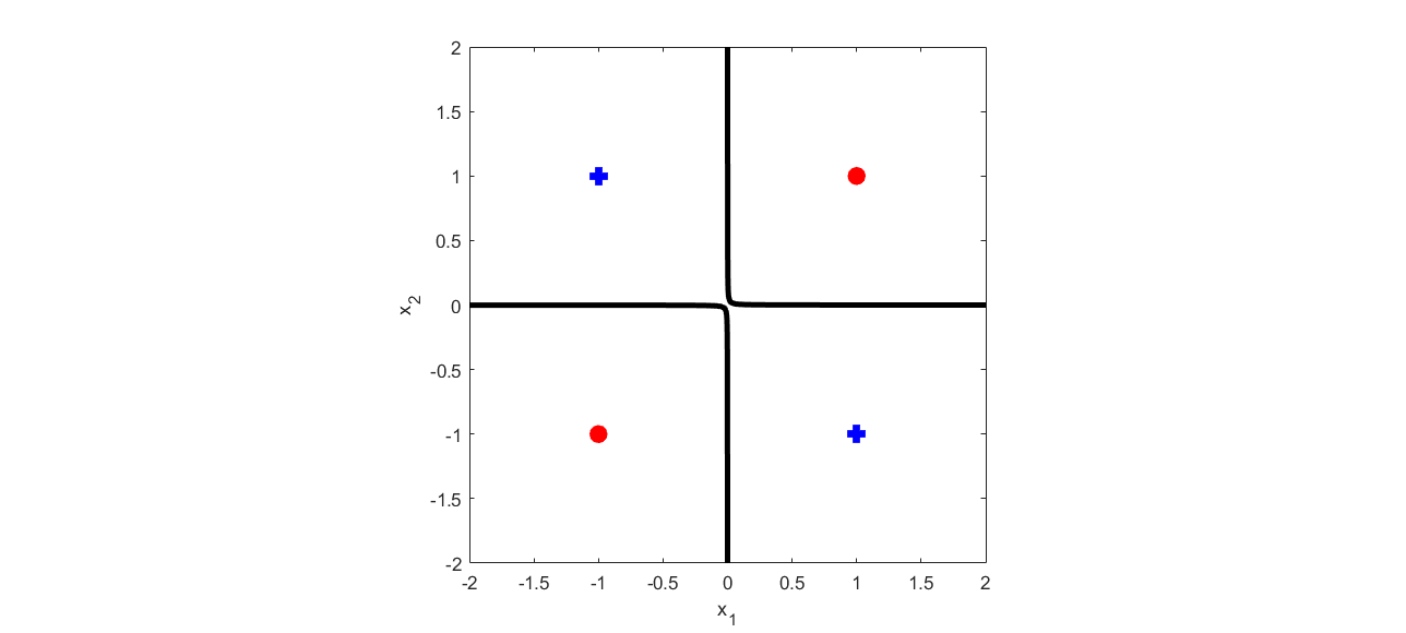
((a))

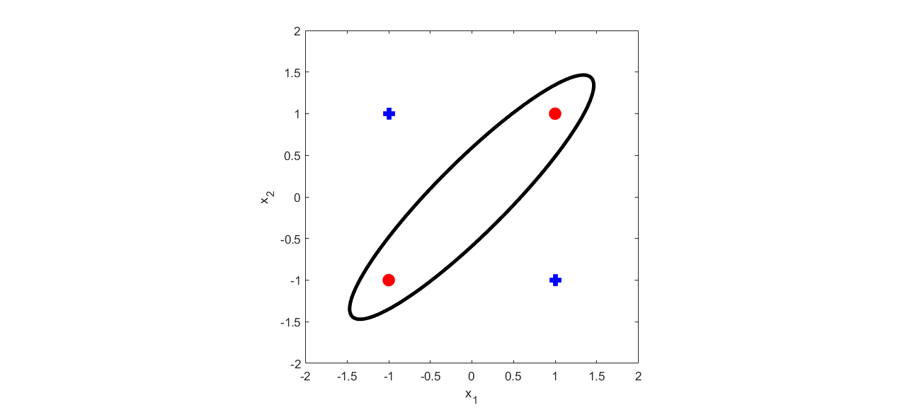
((b))

Figure 1: A single quadratic neuron is able to separate the XOR dataset with a hyperbola or an ellipse. Two possible solutions are shown. (a) When $\mathbf{Q}$ is initalized with a random matrix, a hyperbolic decision boundary was obtained. (b) When $\mathbf{Q}$ is initalized with the Identity matrix, an ellipsoidal decision boundary was obtained.

In the following we consider general feedforward networks consisting of multiple layers of quadratic neurons and derive the vectorized BP algorithm update equations.

III Backpropagation in feedforward artificial neural networks with quadratic neurons

The following notation is used to represent a QNN model.

$$z_{k}^{l} = k l^{th}$$ Total input to the -th neuron in the layer

$$w^{l}_{ki} = i^{th}$$ Weight parameter connecting the neuron in the

$$(l-1)^{th} k^{th} l^{th}$$ layer to the neuron in the layer

$$a^{l}_{k} = k^{th} l^{th}$$ Output of the neuron in the layer

$$a_{k}^{l} = g_{l}(z^{l}_{k});\mbox{ where $g_{l}$ is the activation function used}$$

in the $$l^{th}$$ layer

The quadratically weighted input to the $k$-th neuron in the $l^{th}$ layer is:

$$z^{l}_{k} = b^{l}_{k}+\sum_{i=1}^{n_{l}-1}w^{l}_{ki}a^{l-1}_{i}+\sum_{m=1}^{n_{l}-1}\sum_{n=1}^{n_{l}-1}q_{mn}^{lk}a^{l-1}_{m}a^{l-1}_{n}$$ (26)

$$= b^{l}_{k}+W^{l}_{k:}\mathbf{a}^{l-1}+(\mathbf{a}^{l-1})^{T}Q^{lk}\mathbf{a}^{l-1}$$ (27)

Where $b^{l}_{k}$ are the bias parameters of the $k^{th}$ neuron in the $l^{th}$ layer, $W^{l}_{k:}$ is the $k^{th}$ row vector of $W^{l}$ ($l^{th}$ layer weight matrix) and $\mathbf{a}^{l-1}$ is the vector of outputs from the $(l-1)^{th}$ layer.

Equation (27) can be concisely expressed in vectorized form (29).

$$\mathbf{z}^{l} = \mathbf{b}^{l}+\mathbf{W}^{l}\mathbf{a}^{l-1}$$ (28)

$$+ \begin{bmatrix}(\mathbf{a^{l-1})}^{T}&0&\cdots&0\\ 0&(\mathbf{a^{l-1})}^{T}&\cdots&0\\ \vdots&\vdots&\ddots&\vdots\\ 0&0&\cdots&(\mathbf{a^{l-1})}^{T}\end{bmatrix}\begin{bmatrix}Q^{l1}\\ Q^{l2}\\ \vdots\\ Q^{ln_{l}}\end{bmatrix}\mathbf{a}^{l-1}$$

$$= \mathbf{b}^{l}+\mathbf{W}^{l}\mathbf{a}^{l-1}+\mathbf{A}^{l-1}\mathbf{Q}^{l}\mathbf{a}^{l-1}$$

$$= \mathbf{b}^{l}+(\mathbf{W}^{l}+\mathbf{A}^{l-1}\mathbf{Q}^{l})\mathbf{a}^{l-1}$$ (29)

Where $Q^{lk}=[q_{mn}^{lk}]$ is the matrix of parameters associated with the quadratic term for the $k^{th}$ neuron in the $l^{th}$ layer. The individual $Q^{lk}$ matrices in the $l^{th}$ layer are collected in a single block matrix $\mathbf{Q}^{l}$ for convenience.

Based on the above, the equations for forward propagation in a QNN are summarized in (30).

$$\begin{split}\mathbf{z}^{l}&=\mathbf{b}^{l}+(\mathbf{W}^{l}+\mathbf{A}^{l-1}\mathbf{Q}^{l})\mathbf{a}^{l-1}\\ \mathbf{a}^{l}&=g_{l}(\mathbf{z}^{l})\mbox{ where }l=1,2,3,\cdots,L\end{split}$$ (30)

For generality and simplicity, the non-mutually exclusive multi-label classification task is considered. Cross-entropy (31) is the standard loss function for multi-label classification tasks and we use the same.

$$\mathcal{L}(\mathbf{y},\mathbf{\hat{y}})=-\sum_{p=1}^{n_{L}}\left[y_{p}\ln{\hat{y}_{p}}+(1-y_{p})\ln{(1-\hat{y}_{p})}\right]$$ (31)

The free parameters in the above QNN model are $b^{l}_{k}$, $w_{kj}^{l}$ and $q_{mn}^{lk}$ and which is represented by $\Theta$.

Using the Chain Rule:

$$\frac{\partial\mathcal{L}}{\partial\Theta}=\frac{\partial\mathcal{L}}{\partial z^{l}_{k}}.\frac{\partial z^{l}_{k}}{\partial\Theta}=\delta^{l}_{k}\frac{\partial z^{l}_{k}}{\partial\Theta}.$$ (32)

Since

$$\frac{\partial z^{l}_{k}}{\partial b^{l}_{k}}=1\implies\frac{\partial L}{\partial b^{l}_{k}}=\delta^{l}_{k}$$ (33)

(33) is written in vectorized form below.

$$\frac{\partial\mathcal{L}}{\partial\mathbf{b}^{l}}=\bm{\delta}^{l}$$ (34)

Applying the chain rule again results in (35) and (36):

$$\frac{\partial\mathcal{L}}{\partial w^{l}_{kj}}=\delta^{l}_{k}a^{l-1}_{j}$$ (35)

$$\frac{\partial z^{l}_{k}}{\partial w^{l}_{kj}}=a^{l-1}_{j}$$ (36)

The above results can be expressed in vectorized form (37).

$$\frac{\partial\mathcal{L}}{\partial\mathbf{W}^{l}} = \left[\frac{\partial\mathcal{L}}{\partial w^{l}_{pq}}\right]=[\delta^{l}_{p}a^{l-1}_{q}]$$ (37)

$$= \bm{\delta}^{l}(\mathbf{a}^{l-1})^{T}=\bm{\delta}^{l}\otimes\mathbf{a}^{l-1}$$

The update for $\mathbf{Q}$ can be derived starting from (32).

$$\frac{\partial\mathcal{L}}{\partial q^{lk}_{rs}}=\delta^{l}_{k}\frac{\partial z^{l}_{k}}{\partial q^{lk}_{rs}}$$ (38)

where,

$$\frac{\partial z^{l}_{k}}{\partial q_{rs}^{lk}} = \frac{\partial}{\partial q^{lk}_{rs}}\left[\sum_{m=1}^{n_{l}}\sum_{n=1}^{n_{l}}q^{lk}_{mn}a_{m}^{l-1}a_{n}^{l-1}\right]$$ (39)

$$= \left\{\begin{tabular}[]{lcr}$2a^{l-1}_{r}a^{l-1}_{s}$&if&$r\neq s$\\ $(a_{r}^{l-1})^{2}$&if&$r=s$\end{tabular}\right.$$ (42)

$$\triangleq [m^{lk}_{rs}]$$ (43)

The above equation can be recast as:

$$\frac{\partial\mathcal{L}}{\partial Q^{lk}}=\delta^{l}_{k}M^{lk}$$ (44)

$$M^{lk} \triangleq [m^{lk}_{rs}]$$ (45)

$$= \begin{bmatrix}(a^{l-1}_{1})^{2}&2a_{1}^{l-1}a_{2}^{l-1}&\cdots&2a_{1}^{l-1}a_{n_{l}}^{l-1}\\ 2a^{l-1}_{2}a^{l-1}_{1}&(a_{2}^{l-1})^{2}&\cdots&2a^{l-1}_{2}a^{l-1}_{n_{l}}\\ \vdots&\vdots&\ddots&\vdots\\ 2a^{l-1}_{n_{l}}a^{l-1}_{1}&2a^{l-1}_{n_{l}}a^{l-1}_{2}&\cdots&(a^{l-1}_{n_{l}})^{2}\end{bmatrix}$$ (46)

Now, we consider backpropagating the error to compute $\delta^{l-1}$ from $\delta^{l}$.

$$\delta^{l-1}_{t} = \frac{\partial\mathcal{L}}{\partial z_{t}^{l-1}}$$ (47)

$$= \sum_{k=1}^{n_{l}}\frac{\partial\mathcal{L}}{\partial z^{l}_{k}}.\frac{\partial z^{l}_{k}}{\partial a^{l-1}_{t}}.\frac{\partial a^{l-1}_{t}}{\partial z^{l-1}_{t}}$$ (48)

$$= \sum_{k=1}^{n_{l}}\delta^{l}_{k}\frac{\partial z^{l}_{k}}{\partial a^{l-1}_{t}}g_{l-1}^{\prime}(z^{l-1}_{t})$$ (49)

Since,

$$z^{l}_{k}=b^{l}_{k}+\sum_{i=1}^{n_{l}}w^{l}_{ki}a^{l-1}_{i}+\sum_{m=1}^{n_{l}}\sum_{n=1}^{n_{l}}q^{lk}_{mn}a^{l-1}_{m}a^{l-1}_{n}$$ (50)

$$\frac{\partial z^{l}_{k}}{\partial a^{l-1}_{t}}=w^{l}_{kt}+2\sum_{p}^{n_{l}}q^{lk}_{tp}a^{l-1}_{p}$$ (51)

Substituting (51) in (49), we get:

$$\delta^{l-1}_{t} = \sum_{k=1}^{n_{l}}\delta_{k}^{l}w^{l}_{kt}+2\sum_{p=1}^{n_{l}}(q^{lk}_{tp}a^{l-1}_{p})g_{l-1}^{\prime}(z^{l-1}_{t})$$

$$= g_{l-1}^{\prime}(z^{l-1}_{t})\left[\sum_{k=1}^{n_{l}}\delta^{l}_{k}W^{l}_{kt}+2\sum_{k=1}^{n_{l}}\sum_{p=1}^{n_{l}}\delta^{l}_{k}q_{tp}^{lk}a^{l-1}_{p}\right]$$

$$= g_{l-1}^{\prime}(z^{l-1}_{t})\left[\sum_{k=1}^{n_{l}}(W^{l}_{tk})^{T}\delta_{k}^{l}+2\sum_{k=1}^{n_{l}}\delta_{k}^{l}\sum_{p=1}^{n_{l}}q^{lk}_{tp}a^{l-1}_{p}\right]$$

(LABEL:delta) is presented in vectorized form in (53).

$$\bm{\delta}^{l-1}=g_{l-1}^{\prime}(\mathbf{z}^{l-1})\odot\left[(\mathbf{W}^{l})^{T}\bm{\delta}^{l}+2\sum_{k=1}^{n_{l}}\delta_{k}^{l}Q^{lk}\mathbf{a}^{l-1}\right]$$ (53)

Now, the second term inside the square brackets of (53) is,

$$\sum_{k=1}^{n_{l}}\delta_{k}^{l}(Q^{lk}\mathbf{a}^{l-1})=\begin{bmatrix}Q^{l1}\mathbf{a}^{l-1}&Q^{l2}\mathbf{a}^{l-1}&\cdots&Q^{ln_{l}}\mathbf{a}^{l-1}\end{bmatrix}\bm{\delta}^{l}$$ (54)

Similar to (29):

$$\begin{bmatrix}(\mathbf{a}^{l-1})^{T}Q^{l1}\mathbf{a}^{l-1}\\ (\mathbf{a}^{l-1})^{T}Q^{l2}\mathbf{a}^{l-1}\\ \vdots\\ (\mathbf{a}^{l-1})^{T}Q^{ln_{l}}\mathbf{a}^{l-1}\end{bmatrix}=\mathbf{A}^{l-1}\mathbf{Q}^{l}\mathbf{a}^{l-1}$$ (55)

From (55), we note the following:

$$\mathbf{A}^{l-1}\mathbf{Q}^{l} = \begin{bmatrix}(\mathbf{a}^{l-1})^{T}&0&\cdots&0\\ 0&(\mathbf{a}^{l-1})^{T}&\cdots&0\\ \vdots&\vdots&\ddots&\vdots\\ 0&0&\cdots&(\mathbf{a}^{l-1})^{T}\end{bmatrix}\begin{bmatrix}Q^{l1}\\ Q^{l2}\\ \vdots\\ Q^{ln_{l}}\end{bmatrix}$$ (56)

$$= \begin{bmatrix}(\mathbf{a}^{l-1})^{T}Q^{l1}\\ (\mathbf{a}^{l-1})^{T}Q^{l2}\\ \vdots\\ (\mathbf{a}^{l-1})^{T}Q^{ln_{l}}\end{bmatrix}$$

The transpose of (56) is computed in (57)

$$(\mathbf{A}^{l-1}\mathbf{Q}^{l})^{T} = (\mathbf{Q}^{l})^{T}(\mathbf{A}^{l-1})^{T}$$

$$= \begin{bmatrix}Q^{l1}\\ Q^{l2}\\ \vdots\\ Q^{ln_{l}}\end{bmatrix}^{T}\begin{bmatrix}\mathbf{a}^{l-1}&0&\cdots&0\\ 0&\mathbf{a}^{l-1}&\cdots&0\\ \vdots&\vdots&\ddots&0\\ 0&0&0&\mathbf{a}^{l-1}\end{bmatrix}$$

$$(\mathbf{A}^{l-1}\mathbf{Q}^{l})^{T}=\begin{bmatrix}Q^{l1}\mathbf{a}^{l-1}&Q^{l2}\mathbf{a}^{l-1}&\cdots&Q^{ln_{l}}\mathbf{a}^{l-1}\end{bmatrix}$$ (57)

From (53), (54) and (57), we obtain the vectorized backpropagation update for $\bm{\delta}^{l-1}$ (LABEL:delta_BP).

$$\bm{\delta}^{l-1}=g_{l-1}^{\prime}(\mathbf{z}^{l-1})\odot[(\mathbf{W}^{l})^{T}\bm{\delta}^{l}+2(\mathbf{A}^{l-1}\mathbf{Q}^{l})^{T}\bm{\delta}^{l}]$$

$$\bm{\delta}^{l-1} = g_{l-1}^{\prime}(\mathbf{z}^{l-1})\odot[(\mathbf{W}^{l})^{T}+2(\mathbf{A}^{l-1}\mathbf{Q}^{l})^{T}]\bm{\delta}^{l}$$

(LABEL:delta_BP) for backpropagating $\bm{\delta}^{l}$ clearly reveals the symmetry between forward and backpropagation. The matrix $\mathbf{A}^{l-1}\mathbf{Q}^{l}$ which is the most computationally costly part in forward propagation (30) appears again in transposed form in backpropagation (LABEL:delta_BP). Thus the large matrix $\mathbf{A}^{l-1}\mathbf{Q}^{l}$ can be cached during forward propagation and reused during backpropagation making the this BP algorithm for QNNs computationally efficient.

Letting $\mathbf{V}^{l}=\mathbf{A}^{l-1}\mathbf{Q}^{l}$, the expression for back propagation can be rewritten as in (59).

$$\bm{\delta}^{l-1}=g_{l-1}^{\prime}(\mathbf{z}^{l-1})\odot[(\mathbf{W}^{l})^{T}+2(\mathbf{V}^{l})^{T}]\bm{\delta}^{l}$$ (59)

To start backpropagation, $\bm{\delta}^{l}$ for the last layer namely $\bm{\delta}^{L}$ must first be computed.

For the last layer:

$$a^{L}_{i} = \hat{y}_{i}$$

$$\hat{y}_{i} = \sigma(z^{L}_{i}),\because a_{i}^{L}=\sigma(z^{L}_{i})$$

$$\therefore\frac{\partial\hat{y}_{I}}{\partial z^{L}_{i}} = \hat{y}_{i}(1-\hat{y}_{i})$$

For the last layer, the Chain Rule yields,

$$\delta^{L}_{i} = \frac{\partial\mathcal{L}}{\partial z^{L}_{i}}$$

$$= \frac{\partial\mathcal{L}}{\partial a^{L}_{i}}.\frac{\partial a^{L}_{i}}{\partial z^{L}_{i}}$$

$$= \frac{\partial\mathcal{L}}{\partial\hat{y}_{i}}.\frac{\partial\hat{y}_{i}}{\partial z^{L}_{i}}\because a^{L}_{i}=\hat{y}_{i}$$ (61)

$$= -\left[\frac{y_{i}}{\hat{y}_{i}}-\frac{(1-y_{i})}{(1-\hat{y}_{i})}\right]\hat{y}_{i}(1-\hat{y}_{i})$$ (62)

$$= \hat{y}_{i}-y_{i}$$ (63)

(63) can be written elegantly in vectorized form (64).

$$\bm{\delta}^{L}=\mathbf{\hat{y}}-\mathbf{y}$$ (64)

In Algorithm 1 and Algorithm 2: $\mathbb{D}=\Set{(\mathbf{x}^{i},\mathbf{y}^{i})}{i=1\dots N}$ is the training dataset. Based on the above equations, the training algorithm for QNNs is presented in Algorithm 1.

Algorithm 1 QNN Training Algorithm

  TRAIN_QNN$(\mathbb{D})$

  Initialize: $\eta,\Set{\mathbf{Q}^{l},\mathbf{W}^{l},\mathbf{b}^{l}}{l=1,2,\dots,L}$

   Iterate till convergence

      % Forward Propagation

        $\mathbf{a}^{1}\leftarrow\mathbf{x}^{i}$

        for $l=1,2,...,L$

            $\mathbf{z}^{l}\leftarrow\mathbf{b}^{l}+(\mathbf{W}^{l}+\mathbf{A}^{l-1}\mathbf{Q}^{l})\mathbf{a}^{l-1}$   % Cache for BP

            $\mathbf{a}^{l}\leftarrow g(\mathbf{z}^{l})$ % Cache for BP

            $\mathbf{V}^{l}\leftarrow\mathbf{A}^{l-1}\mathbf{Q}^{l}$ % Cache for BP

        endfor

        $\mathbf{\hat{y}}\leftarrow\mathbf{a}^{L}$

        $\bm{\delta}^{L}\leftarrow\mathbf{\hat{y}}-\mathbf{y}^{i}$

      % Backward Propagation

        for $l=L,L-1,\dots,2$

            $\bm{\delta}^{l-1}=g_{l-1}^{\prime}(\mathbf{z}^{l-1})\odot[(\mathbf{W}^{l})^{T}+2(\mathbf{V}^{l})^{T}]\bm{\delta}^{l}$

        endfor

        for $l=1,2,\dots,L$

            $\mathbf{b}^{l}\leftarrow\mathbf{b}^{l}-\eta\bm{\delta}^{l}$

            $\mathbf{W}^{l}\leftarrow\mathbf{W}^{l}-\eta\bm{\delta}^{l}\otimes\mathbf{a}^{l-1}$

            $\mathbf{Q}^{l}\leftarrow\mathbf{Q}^{l}-\eta\bm{\delta}^{l}\mathbf{M}(\mathbf{a}^{l-1})$

        endfor

            $i\leftarrow i+1$

   return $\Set{\mathbf{Q}^{l},\mathbf{W}^{l},\mathbf{b}^{l}}{l=1,2,\dots,L}$

Next a reduced parameter QNN model that provides a compromise between model complexity and representation power is proposed.

IV Reduced Parameter Quadratic Neural Networks (RPQNN)

One possible approach for reducing the number of parameters in the standard quadratic neuron model is to consider only quadratic functions that are product of the affine functions. In this model each neuron with $n$ inputs has only $2n$ additional parameters instead of $\frac{n(n+1)}{2}$. In the following a new Reduced Parameter Quadratic Neural Networks (RPQNN) model is proposed.

The output of layer $l$ in the RPQNN is calculated as follows:

$$z_{i}^{l} = (W_{i:}\mathbf{a}^{l-1}+b_{i}^{l})(U^{l}_{i:}\mathbf{a}^{l-1}+c_{i}^{l})$$ (65)

$$\mathbf{z}^{l} = (\mathbf{W}^{l}\mathbf{a}^{l-1}+\mathbf{b}^{l})\odot(\mathbf{U}^{l}\mathbf{a}^{l-1}+\mathbf{c}^{l})$$ (66)

$$\mathbf{a}^{l} = g_{l}(\mathbf{z}^{l})$$ (67)

Algorithm 2 RPQNN Training Algorithm

  TRAIN_RPQNN($\mathbb{D}$)

  Initialize: $\eta,\Set{\mathbf{W}^{l},\mathbf{U}^{l},\mathbf{b}^{l},\mathbf{c}^{l}}{l=1,2,\dots,L}$

   Iterate till convergence

      % Forward Propagation

      $\mathbf{a}^{1}\leftarrow\mathbf{x}^{i}$

        for $l=1,2,...,L$

            $\mathbf{v}_{1}^{l}\leftarrow(\mathbf{W}^{l}\mathbf{a}^{l-1}+\mathbf{b}^{l})$   % Cache for BP

            $\mathbf{v}_{2}^{l}\leftarrow(\mathbf{U}^{l}\mathbf{a}^{l-1}+\mathbf{c}^{l})$   % Cache for BP

            $\mathbf{z}^{l}\leftarrow\mathbf{v}^{l}_{1}\odot\mathbf{v}^{l}_{2}$   % Cache for BP

            $\mathbf{a}^{l}\leftarrow g(\mathbf{z}^{l})$   % Cache for BP

        endfor

        $\mathbf{\hat{y}}\leftarrow\mathbf{a}^{L}$

        $\bm{\delta}^{L}\leftarrow\mathbf{\hat{y}}-\mathbf{y}^{i}$

      % Backward Propagation

        for $l=L,L-1,\dots,2$

            $\bm{\delta}^{l-1}\leftarrow g^{\prime}_{l-1}(\mathbf{z}^{l-1})\odot[(\mathbf{U}^{l})^{T}(\bm{\delta}^{l}\odot\mathbf{v}_{1}^{l})+(\mathbf{W}^{l})^{T}(\bm{\delta}^{l}\odot\mathbf{v}_{2}^{l})]$

        endfor

        for $l=1,2,\dots,L$

            $\mathbf{b}^{l}\leftarrow\mathbf{b}^{l}-\eta\bm{\delta}^{l}\odot\mathbf{v}^{l}_{1}$

            $\mathbf{c}^{l}\leftarrow\mathbf{c}^{l}-\eta\bm{\delta}^{l}\odot\mathbf{v}^{l}_{2}$

            $\mathbf{W}^{l}\leftarrow\mathbf{W}^{l}-\eta(\bm{\delta}^{l}\odot\mathbf{v}_{2}^{l})\otimes\mathbf{a}^{l-1}$

            $\mathbf{U}^{l}\leftarrow\mathbf{U}^{l}-\eta(\bm{\delta}^{l}\odot\mathbf{v}_{1}^{l})\otimes\mathbf{a}^{l-1}$

        endfor

      $i\leftarrow i+1$

   return $\Set{\mathbf{W}^{l},\mathbf{U}^{l},\mathbf{b}^{l},\mathbf{c}^{l}}{l=1,2,\dots,L}$

The parameters $\Theta$ are $w_{ij}^{l}$, $b^{l}_{i}$, $u^{l}_{ij}$ and $c^{l}_{i}$.

Using the Chain Rule (68) :

$$\frac{\partial\mathcal{L}}{\partial w^{l}_{ij}}=\frac{\partial\mathcal{L}}{\partial z^{l}_{i}}\frac{\partial z^{l}_{i}}{\partial w_{ij}^{l}}=\delta^{l}_{i}\frac{\partial z^{l}_{i}}{\partial w^{l}_{ij}}$$ (68)

$$\frac{\partial z^{l}_{i}}{\partial w^{l}_{ij}}=(U^{l}_{i:}\mathbf{a}^{l-1}+c_{i}^{l})a_{j}^{l-1}$$ (69)

$$\frac{\partial\mathcal{L}}{\partial w^{l}_{ij}}=\delta^{l}_{i}(U_{i:}^{l}\mathbf{a}^{l-1}+c_{i}^{l})a_{j}^{l-1}$$ (70)

Using the concept of matrix derivatives, the above weight update equations (70) can be vectorized and presented concisely as follows (71):

$$\frac{\partial\mathcal{L}}{\partial\mathbf{W}^{l}}=[\bm{\delta}^{l}\odot(\mathbf{c}^{l}+\mathbf{U}^{l}\mathbf{a}^{l-1})]\otimes\mathbf{a}^{l-1}$$ (71)

By symmetry, we obtain the gradient with respect to $\mathbf{U}$ (72):

$$\frac{\partial\mathcal{L}}{\partial\mathbf{U}^{l}}=[\bm{\delta}^{l}\odot(\mathbf{b}^{l}+\mathbf{W}^{l}\mathbf{a}^{l-1})]\otimes\mathbf{a}^{l-1}$$ (72)

Next the gradient of $\mathbf{b}$ which can be calculated as shown below (73)

$$\frac{\partial\mathcal{L}}{\partial b^{l}_{i}}=\frac{\partial\mathcal{L}}{\partial z^{l}_{i}}\frac{\partial z^{l}_{i}}{\partial b^{l}_{i}}=\delta^{l}_{i}(c^{l}_{i}+U_{i:}\mathbf{a}^{l-1})$$ (73)

(73) can be vectorized to yield (74)

$$\frac{\partial\mathcal{L}}{\partial\mathbf{b}^{l}}=\bm{\delta}^{l}\odot(\mathbf{c}^{l}+\mathbf{U}^{l}\mathbf{a}^{l-1})$$ (74)

By symmetry with (74), the grdient of $\mathbf{c}$ is (75)

$$\frac{\partial\mathcal{L}}{\partial\mathbf{c}^{l}}=\bm{\delta}^{l}\odot(\mathbf{b}^{l}+\mathbf{W}^{l}\mathbf{a}^{l-1})$$ (75)

Next we consider the equation for backpropagating $\bm{\delta}^{l}$. Using the multivariable Chain Rule:

$$\delta^{l-1}_{i} = \frac{\partial L}{\partial z_{i}^{l-1}}$$ (76)

$$= \sum_{k}^{n_{l}}\frac{\partial L}{\partial z_{k}^{l}}\frac{\partial z_{k}^{l}}{\partial a^{l-1}_{i}}\frac{\partial a^{l-1}_{i}}{\partial z^{l-1}_{i}}$$

(76) can be simplified to obtain (77).

$$\delta^{l-1}_{i}=g_{l-1}^{\prime}(z_{i}^{l-1})\sum_{k=1}^{n_{l}}\delta_{k}^{l}\frac{\partial z^{l}_{k}}{\partial a^{l-1}_{i}}$$ (77)

Now, $\frac{\partial z^{l}_{k}}{\partial a^{l-1}_{i}}$ in (77) can be calculated as follows:

$$\frac{\partial z_{k}^{l}}{\partial a_{i}^{l-1}} = \frac{\partial}{\partial a_{i}^{l-1}}\left[(b_{k}^{l}+W_{k:}^{l}\mathbf{a}^{l-1})(c_{k}^{l}+U_{k:}^{l}\mathbf{a}^{l-1})\right]$$

$$= \frac{\partial}{\partial a_{i}^{l-1}}\left[b_{k}^{l}(U_{k:}^{l}\mathbf{a}^{l-1})+c_{k}^{l}(W_{k:}\mathbf{a}^{l-1})\right.$$

$$+ \left.(W_{k:}^{l}\mathbf{a}^{l-1})(U^{l}_{k:}\mathbf{a}^{l-1})\right]$$

$$\frac{\partial z_{k}^{l}}{\partial a_{i}^{l-1}} = b^{l}_{k}u^{l}_{ki}+c_{k}^{l}w_{ki}^{l}+w_{ki}^{l}(U_{k:}^{l}\mathbf{a}^{l-1})$$ (78)

$$+ u_{ki}^{l}(W_{k:}^{l}\mathbf{a}^{l-1})$$

Substituting (78) in (77) we get:

$$\delta_{i}^{l-1} = g_{l-1}^{\prime}(z_{i}^{l-1})\sum_{k=1}^{n_{l}}\left[\delta_{k}^{l}b_{k}^{l}u_{ki}^{l}+\delta_{k}^{l}c_{k}^{l}w_{ki}^{l}\right.$$ (79)

$$+ \delta_{k}^{l}w_{ki}^{l}(U_{k:}^{l}\mathbf{a}^{l-1})+\delta_{k}^{l}u_{ki}^{l}(W_{k:}^{l}\mathbf{a}^{l-1})]$$

(79) can be vectorized and expressed in compact and computationally efficient form (80).

$$\bm{\delta}^{l-1} = g_{l-1}^{\prime}(\mathbf{z}^{l-1})$$

$$\odot \left[(\mathbf{U}^{l})^{T}(\bm{\delta}^{l}\odot\mathbf{b}^{l})\right.$$

$$+ (\mathbf{W}^{l})^{T}(\bm{\delta}^{l}\odot\mathbf{c}^{l})$$

$$+ (\mathbf{W}^{l})^{T}(\bm{\delta}^{l}\odot\mathbf{U}^{l}\mathbf{a}^{l-1})$$

$$+ \left.(\mathbf{U}^{l})^{T}(\bm{\delta}^{l}\odot\mathbf{W}^{l}\mathbf{a}^{l-1})\right]$$

$$= g^{\prime}(\mathbf{z}^{l-1})\odot\left[(\mathbf{U}^{l})^{T}\left[\bm{\delta}^{l}\odot\mathbf{b}^{l}+\bm{\delta}^{l}\odot\mathbf{W}^{l}\mathbf{a}^{l-1}\right]\right.$$

$$\hskip 11.38092pt+(\mathbf{W}^{l})^{T}\left.\left[\bm{\delta}^{l}\odot\mathbf{c}^{l}+\bm{\delta}^{l}\odot\mathbf{U}^{l}\mathbf{a}^{l-1}\right]\right]$$

$$= g^{\prime}(\mathbf{z}^{l-1})\odot\left[(\mathbf{U}^{l})^{T}\left[\bm{\delta}^{l}\odot(\mathbf{W}^{l}\mathbf{a}^{l-1}+\mathbf{b}^{l})\right]\right.$$

$$\hskip 11.38092pt+(\mathbf{W}^{l})^{T}\left.\left[\bm{\delta}^{l}\odot(\mathbf{U}^{l}\mathbf{a}^{l-1}+\mathbf{c}^{l})\right]\right.$$

$$\bm{\delta}^{l-1} = g^{\prime}_{l-1}(\mathbf{z}^{l-1})\odot\left\{(\mathbf{U}^{l})^{T}\left[\bm{\delta}^{l}\odot(\mathbf{W}^{l}\mathbf{a}^{l-1}+\mathbf{b}^{l})\right]\right.$$ (80)

$$\hskip 39.83368pt+(\mathbf{W}^{l})^{T}\left.\left[\bm{\delta}^{l}\odot(\mathbf{U}^{l}\mathbf{a}^{l-1}+\mathbf{c}^{l})\right]\right\}$$

The quantities $\mathbf{W}^{l}\mathbf{a}^{l-1}+\mathbf{b}^{l}$ and $\mathbf{U}^{l}\mathbf{a}^{l-1}+\mathbf{c}^{l}$ can be cached during Forward Propagation and reused during Backpropagation making this model computationally efficient. Based on the above equations, the training algorithm for RQNNS is presented in Algorithm 2.

V Results and Discussion

In this section, we compare the performance of QNNs and standard ANNs on the following 3 benchmark classification datasets:

1. Nonlinear Cluster dataset

2. MNIST dataset

3. Diabetes dataset

The final classification test-accuracy is a random variable due to the random weight and bias initialization at the start of training. Due to the random parameter initialization, gradient descent starts at a different point in the parameters space and reaches possibly different local minimum every time the model ins trained. So, in the following, the average accuracy over 25 independent training sessions starting from initial random weights and biases is considered to average out the variation in test-accuracy due to the random initialization.

V-A Performance on a Nonlinear Cluster dataset

Fig. 2 shows a 6-cluster linearly non-separable dataset. The clusters were generated using 2D Gaussian random variables with mean and covariance matrix given in Table I. The Nonlinear Cluster dataset consists of 6 classes and a training dataset consisting of 2000 training pairs per class. The test dataset consists of 3000 training pairs with 500 pairs for each of the 6 classses. A single layer QNN consisting of 6 quadratic neurons was trained using (9), (12) and (24) for 10000 epochs with a learning rate of 0.0001 Nonlinear Cluster dataset. With the above settings, the test-accuracy was observed to be $99.97\%$. Fig. 2 shows the different classes and the decision boundaries of the 6 neurons in the single layer QNN in different colors. This dataset demonstrates that single layer QNNs can learn complex nonlinear quadric boundaries that a standard single layer ANN cannot learn. The decision boundaries of the QNN in this 2-dimensional example are ellipses and hyperbolas. In n-dimension the decision boundaries of the QNN will be general quadric surfaces of the form ($\mathbf{x}^{T}\mathbf{Q}\mathbf{x}+\mathbf{w}^{T}\mathbf{x}+b=0$). An hyper-ellipsoidal decision boundary can always be found such that $\mathbf{x}^{T}\mathbf{Q}\mathbf{x}+\mathbf{w}^{T}\mathbf{x}+b>0$ for inputs belonging to a bounded cluster and $\mathbf{x}^{T}\mathbf{Q}\mathbf{x}+\mathbf{w}^{T}\mathbf{x}+b<0$ for inputs not belonging to the cluster. Since the boundary of a quadratic neuron can be an arbitrary hyper-ellipsoid it is clear that any bounded $C$ clusters dataset requires only a single layer QNN with $C$ neurons. This problem clearly demonstrates that single layer QNNs can solve problems that can only be solved using standard ANNs with hidden layers.

TABLE I: Nonlinear Cluster dataset

Color	Red	Black	Magenta	Green	Cyan	Blue
Mean	(-16,0)	(-8,0)	(0,0)	(0,10)	(-8,10)	(-16,10)
Covariance	$\begin{bmatrix}1&-0.3\\ -0.3&1\end{bmatrix}$	$\begin{bmatrix}1&0\\ 0&1\end{bmatrix}$	$\begin{bmatrix}1&0.3\\ 0.3&1\end{bmatrix}$	$\begin{bmatrix}1&-0.3\\ -0.3&1\end{bmatrix}$	$\begin{bmatrix}1&0\\ 0&1\end{bmatrix}$	$\begin{bmatrix}1&0.3\\ 0.3&1\end{bmatrix}$

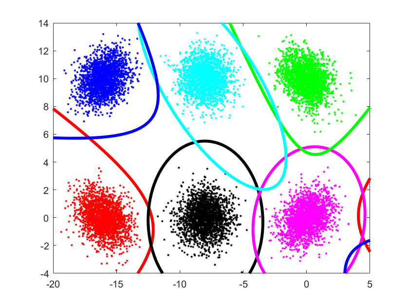
Figure 2: A dataset that is not linearly separable and consisting of 6 scatters. Different classes and the associated decision boundary of a single layer 6 neuron QNN that was successfully able to learn this dataset.

V-B Performance on MNIST

In the following, the performance of QNN, RPQNN and standard ANN models is compared on the widely used MNIST benchmark dataset [15]. MNIST provides a training set of 60,000 labeled 28 by 28 pixel images of the 10 handwritten digits (0 to 9) and test-dataset of 10,000 images. A simple 2 layer feedforward ANN model was considered. All models had 784 inputs (flattened 28 by 28 pixel images), a single hidden layer composed of logistic sigmoidal neurons and a 10 neuron output layer. For the ANN model, the output layer consisted of 10 logistic sigmoidal neurons and for the QNN and RPQNN models the output layer consisted of a 10 sigmoidal neuron QNN and RPQNN layer respectively. The different models were trained with the SGD algorithm and a learning rate of 0.01 was used. Table II shows the accuracy achieved with different number of hidden layer neurons by the ANN and QNN models. Table II clearly indicates that the QNN achieves notably higher accuracy on MNIST. In particular it is impressive that the QNN achieves an accuracy exceeding 80% with just 5 hidden neurons and an accuracy exceeding 90% with just 10 hidden neurons. Table II compares the performance of the ANN, QNN and RPQNN models on the MNIST benchmark. Table II presents the mean, standard deviation, the best and worst accuracy for 25 independent trials. The results presented in Table II clearly demonstrate the superior performance of QNNs and RPQNNs even with reduced number of identical hidden layer neurons. In particular it is interesting to note that the QNN models achieve an accuracy exceeding 81% with just 5 hidden neurons. The above results indicate that QNNs and RPQNNs perform significantly better when the number of hidden layer neurons is low. When the number of hidden layer neurons is increased beyond a certain number, the features become linearly separable and complex quadric surfaces are no longer needed to separate the classes.

TABLE II: Comparison of ANN, QNN and RPQNN models on MNIST

Max	Hidden	ANN		QNN		RPQNN
Epochs	Neurons	$\mu\pm\sigma$	Best/Worst	$\mu\pm\sigma$	Best/Worst	$\mu\pm\sigma$	Best/Worst
1	5	74.86 $\pm$ 3.56	79.79/66.71	81.11 $\pm$ 3.78	86.09/69.24	81.13 $\pm$ 3.49	87.55/74.17
	10	88.69 $\pm$ 0.74	89.84/86.67	90.03 $\pm$ 0.91	91.49/87.05	89.02 $\pm$ 1.03	91.24/86.58
	15	90.39 $\pm$ 0.34	91.02/89.55	92.19 $\pm$ 0.63	93.11/90.58	90.72 $\pm$ 0.98	92.10/88.32
	20	90.79 $\pm$ 0.39	91.42/89.82	93.11 $\pm$ 0.55	93.92/91.46	91.47 $\pm$ 0.84	92.82/89.34
	25	91.03 $\pm$ 0.36	91.56/90.06	93.46 $\pm$ 0.78	94.32/90.93	92.22 $\pm$ 0.47	93.02/91.04
	30	91.26 $\pm$ 0.39	91.85/90.42	93.74 $\pm$ 0.50	94.50/92.55	92.52 $\pm$ 0.65	93.44/91.22
4	5	84.81 $\pm$ 1.35	86.87/80.85	85.87 $\pm$ 1.04	87.66/83.76	85.78 $\pm$ 1.53	88.13/80.56
	10	90.88 $\pm$ 0.61	91.93/89.41	92.12 $\pm$ 0.78	93.41/90.39	91.31 $\pm$ 0.67	92.30/89.74
	15	92.62 $\pm$ 0.40	93.54/91.77	94.26 $\pm$ 0.44	95.23/93.12	93.31 $\pm$ 0.41	94.15/92.48
	20	93.57 $\pm$ 0.31	94.17/93.00	95.30 $\pm$ 0.37	95.76/93.92	93.94 $\pm$ 0.54	94.85/92.56
	25	94.06 $\pm$ 0.26	94.50/93.59	95.77 $\pm$ 0.32	96.21/94.87	94.65 $\pm$ 0.41	95.21/93.54
	30	94.59 $\pm$ 0.29	95.01/93.68	96.24 $\pm$ 0.38	96.84/95.31	95.18 $\pm$ 0.51	95.81/93.66
20	5	87.21 $\pm$ 1.13	89.06/84.12	87.07 $\pm$ 0.93	88.82/85.32	87.50 $\pm$ 1.25	89.39/82.86
	10	87.21 $\pm$ 1.13	89.06/84.12	87.07 $\pm$ 0.93	88.82/85.32	87.50 $\pm$ 1.25	89.39/82.86
	15	93.51 $\pm$ 0.39	94.15/92.64	94.84 $\pm$ 0.54	95.44/92.61	94.00 $\pm$ 0.40	94.66/93.17
	20	94.78 $\pm$ 0.28	95.25/94.16	95.92 $\pm$ 0.22	96.29/95.46	95.00 $\pm$ 0.28	95.60/94.41
	25	95.43 $\pm$ 0.20	95.72/95.05	96.50 $\pm$ 0.31	96.98/95.75	95.73 $\pm$ 0.26	96.17/95.19
	30	95.97 $\pm$ 0.18	96.31/95.55	96.97 $\pm$ 0.23	97.38/96.52	96.11 $\pm$ 0.31	96.61/95.56
200	5	87.12 $\pm$ 0.96	88.94/85.17	87.43 $\pm$ 0.96	89.14/85.56	87.26 $\pm$ 0.88	88.89/86.04
	10	92.07 $\pm$ 0.35	92.74/91.41	92.88 $\pm$ 0.43	93.77/91.97	92.37 $\pm$ 0.50	93.63/91.37
	15	93.84 $\pm$ 0.37	94.61/93.25	94.64 $\pm$ 0.32	95.05/93.43	93.93 $\pm$ 0.29	94.53/93.22
	20	94.70 $\pm$ 0.18	95.16/94.37	95.53 $\pm$ 0.19	95.93/95.11	94.83 $\pm$ 0.26	95.31/94.26
	25	95.33 $\pm$ 0.19	95.58/94.99	96.25 $\pm$ 0.18	96.49/95.87	95.35 $\pm$ 0.22	96.05/95.56
	30	95.76 $\pm$ 0.22	96.12/95.30	96.89 $\pm$ 0.17	97.15/96.53	95.74 $\pm$ 0.25	96.12/95.08

V-C Performance on Diabetes dataset

In the following, we compare the performance of QNN and standard ANN models on a structured (tabular) dataset. Unstructured datasets like MNIST have inputs with homogeneous features such as images where all the input features are pixel values from 0 to 255. Structured datasets are more challenging because the input features in structured data are heterogeneous arising from different sources and measured in disparate units. The Diabetes dataset [16] is a challenging benchmark involving tabular data. The Diabetes dataset contains tabular type data with 21 input features and 3 target classes corresponding to no-diabetes, pre-diabetes and diabetes. The 21 input features in this dataset are a mix of categorical and non-categorical variables. There are a total of 253680 instances in the Diabetes dataset and 80% of the instances were used for training and the remaining 20% of the instances were used for testing. The performance of three models, an ANN model, QNN and a RPQNN model were compared. A simple 2 layer feedforward ANN model was considered. All models had 21 inputs, a single hidden layer composed of logistic sigmoidal neurons and an output layer consisting of 3 neurons. For the ANN model the output layer consisted of 3 logistic sigmoidal neurons and for the QNN and RPQNN models, the output layer consisted of 3 quadratic neurons. The different models were trained with the SGD algorithm and a learning rate of 0.01 was used. It is clear from Table III that both QNN and RPQNN models outperform the standard ANN model on the challenging Diabetes benchmark.

TABLE III: Comparison of ANN, QNN and RPQNN models on the Diabetes dataset

Max	Hidden	ANN		QNN		RPQNN
Epochs	Neurons	$\mu\pm\sigma$	Best/Worst	$\mu\pm\sigma$	Best/Worst	$\mu\pm\sigma$	Best/Worst
1	5	84.61 $\pm$ 0.06	84.75/84.50	84.58 $\pm$ 0.07	84.70/84.44	84.59 $\pm$ 0.08	84.72/84.43
	10	84.63 $\pm$ 0.05	84.76/84.56	84.64 $\pm$ 0.07	84.76/84.49	84.62 $\pm$ 0.06	84.73/84.50
	15	84.62 $\pm$ 0.06	84.81/84.48	84.68 $\pm$ 0.05	84.76/84.57	84.62 $\pm$ 0.07	84.81/84.41
	20	84.60 $\pm$ 0.05	84.71/83.51	84.69 $\pm$ 0.05	84.77/84.56	84.81$\pm$ 0.10	84.93/84.59
	25	84.60 $\pm$ 0.06	84.72/84.51	84.70 $\pm$ 0.05	84.84/84.56	84.64 $\pm$ 0.07	84.76/84.49
	30	84.58 $\pm$ 0.06	84.70/84.43	84.70 $\pm$ 0.05	84.41/84.56	84.59 $\pm$ 0.08	84.70/84.39
4	5	84.64 $\pm$ 0.06	84.76/84.53	84.66 $\pm$ 0.04	84.75/84.57	84.67 $\pm$ 0.04	84.73/84.59
	10	84.70 $\pm$ 0.05	84.82/84.62	84.72 $\pm$ 0.04	84.77/84.65	84.70 $\pm$ 0.04	84.76/84.57
	15	84.69 $\pm$ 0.05	84.76/84.56	84.73 $\pm$ 0.03	84.78/84.67	84.73 $\pm$ 0.03	84.78/84.65
	20	84.67 $\pm$ 0.05	84.77/84.55	84.75 $\pm$ 0.03	84.80/84.67	84.74 $\pm$ 0.04	84.82/84.67
	25	84.66 $\pm$ 0.05	84.76/84.57	84.74 $\pm$ 0.04	84.81/84.65	84.73 $\pm$ 0.06	84.83/84.65
	30	84.65 $\pm$ 0.05	84.73/84.50	84.75 $\pm$ 0.03	84.82/84.70	84.73 $\pm$ 0.05	84.81/84.62
20	5	84.66 $\pm$ 0.06	84.78/84.50	84.69 $\pm$ 0.03	84.75/84.61	84.67 $\pm$ 0.06	84.77/84.50
	10	84.74 $\pm$ 0.05	84.84/84.62	84.76 $\pm$ 0.05	84.86/84.67	84.73 $\pm$ 0.06	84.84/84.64
	15	84.71 $\pm$ 0.04	84.78/84.64	84.78 $\pm$ 0.04	84.84/84.70	84.75 $\pm$ 0.04	84.83/84.68
	20	84.72 $\pm$ 0.07	84.91/84.60	84.77 $\pm$ 0.05	84.86/84.65	84.75 $\pm$ 0.04	84.83/84.66
	25	84.71 $\pm$ 0.05	84.77/84.59	84.79 $\pm$ 0.03	84.84/84.72	84.78 $\pm$ 0.05	84.87/84.67
	30	84.67 $\pm$ 0.05	84.75/84.56	84.77 $\pm$ 0.04	84.86/84.71	84.86 $\pm$ 0.04	84.84/84.65
200	5	84.67 $\pm$ 0.04	84.76/84.59	84.70 $\pm$ 0.04	84.76/84.56	84.69 $\pm$ 0.06	84.77/84.58
	10	84.75 $\pm$ 0.04	84.82/84.69	84.77 $\pm$ 0.05	84.89/84.69	84.80 $\pm$ 0.05	84.87/84.65
	15	84.74 $\pm$ 0.05	84.86/84.64	84.77 $\pm$ 0.05	84.84/84.68	84.81 $\pm$ 0.05	84.91/84.72
	20	84.71 $\pm$ 0.07	84.85/84.53	84.75 $\pm$ 0.06	84.92/84.65	84.79 $\pm$ 0.04	84.86/84.70
	25	84.69 $\pm$ 0.06	84.79/84.55	84.75 $\pm$ 0.04	84.82/84.69	84.76 $\pm$ 0.07	84.86/84.57
	30	84.66 $\pm$ 0.05	84.74/84.57	84.69 $\pm$ 0.06	84.78/84.57	84.74 $\pm$ 0.05	84.83/84.61

In summary, since each quadratic neuron in a QNN can have a quadric surface as its decision boundary instead of simple hyperplanes, we expect even single layer QNNs to have the representative power of larger ANNs with multiple hidden layers. In particular a single 3-input quadratic neuron can have any one of 17 different quadrics [14] as its decision boundary. For an n-input quadratic neuron (where n is large), the decision boundary can be one of a very large number of possible hyper-quadric surfaces. Many datasets that are not linearly separable can be separated by hyper-quadrics, allowing QNNs to learn many classification tasks without any hidden layers or with reduced number of hidden layer neurons. Fig. 2 shows a complex dataset with 6 classes that are not linearly separable. A single layer of 6 quadratic neurons was able to successfully learn this dataset. The decision boundaries of the individual neurons are also shown in Fig. 2. It is clear from Section V-A than any dataset composed of $C$ clusters requires only a single layer QNN with $C$ neurons. In particular, this is because any bounded cluster can always be separated from other bounded clusters in the dataset using hyper ellipsoids or hyperbolas.

VI Conclusion

This paper explored the advantages of using quadratic neurons in feedforward neural networks. Quadratic neurons are sparse in terms of parameters compared to other higher order neurons because every quadratic form can be represented by a symmetric matrix. Efficient vectorized update equations for a new Quadratic Regression model was presented and single quadratic neurons were shown to possess the ability to learn the XOR function like recently discovered human neocortical pyramidal neurons involved in higher order functions [1]. Efficient vectorized update equations for forward and backpropagation in networks composed of quadratic neurons was presented for the first time in this paper. The BP algorithm for QNNs in matrix form clearly revealed the symmetry between forward and backpropagation (matrices occur as transposes). This paper showed that any dataset consisting only of bounded clusters can be classified by a single layer QNN efficiently. Further the number of quadratic neurons needed to classify a dataset consisting of $C$ bounded clusters is exactly $C$. In a typical ANN, the initial layers perform feature extraction and the later fully connected layers transform the extracted features to make them linearly separable at the final Softmax layer. However since quadratic neurons can separate their inputs with general quadric surfaces instead of simple hyperplanes, fewer neurons are need in the hidden layers when the final layer consists of quadratic neurons. In particular an accuracy exceeding 90 percent was achieved on the MNIST dataset with just a single hidden layer of 10 sigmoidal neurons. QNNs were observed to achieve significantly higher accuracy than conventional ANNs on the MNIST dataset. Results indicate that a final layer of quadratic sigmoidal neurons can significantly reduce the number of hidden layer neurons in ANNs. A reduced parameter QNN called RPQNN architecture was proposed and shown to be computationally efficient. In particular it is shown that the results of computationally expensive matrix operations in forward propagation can be cached and reused during backpropagation. Rapid progress in the development of efficient parallel hardware for training neural networks will enable increasingly deep QNNs to be trained. Future research will explore the possible advantages of using QNNs instead of standard fully connected ANNs for the final layers in CNNs, LSTMs and Transformer models.

References

- [1] Gidon A, Zolnik TA, Fidzinski P, Bolduan F, Papoutsi A, Poirazi P, Holtkamp M, Vida I, Larkum ME. Dendritic action potentials and computation in human layer 2/3 cortical neurons. Science. 2020 Jan 3;367(6473):83-87. doi: 10.1126/science.aax6239. PMID: 31896716.
- [2] Noel, Matthew Mithra, et al. ”Biologically inspired oscillating activation functions can bridge the performance gap between biological and artificial neurons.” arXiv preprint arXiv:2111.04020, 2021.
- [3] Noel, Mathew Mithra, Advait Trivedi, and Praneet Dutta. ”Growing cosine unit: A novel oscillatory activation function that can speedup training and reduce parameters in convolutional neural networks.” arXiv preprint arXiv:2108.12943, 2021.
- [4] A.G. Ivakhnenko, Polynomial theory of complex systems, IEEE transactions on Systems, Man, and Cybernetics, Vol.1, No.4, pp.364–378. 1971.
- [5] C. Lee Giles and Tom Maxwell, ”Learning, invariance, and generalization in high-order neural networks,” Appl. Opt. 26, 4972-4978, 1987.
- [6] M. D. Alder and Y. Attikiouzel, ”Automatic extraction of strokes by quadratic neural nets,” [Proceedings 1992] IJCNN International Joint Conference on Neural Networks, Baltimore, MD, USA, 1992, pp. 559-564 vol.1, doi: 10.1109/IJCNN.1992.287153.
- [7] C. L. Giles and T. Maxwell, Learning, invariance, and generalization in high-order neural networks, Vol. 26, pp.4972–4978, 1987.
- [8] S. M. Fakhraie and K. C. Smith, ”Generalized artificial neural networks (GANN),” Proceedings of Canadian Conference on Electrical and Computer Engineering, Vancouver, BC, Canada, 1993, pp. 469-472 vol.1, doi: 10.1109/CCECE.1993.332192.
- [9] G. S. Lim, M. Alder and P. Hadingham, ”Adaptive quadratic neural nets,” [Proceedings] 1991 IEEE International Joint Conference on Neural Networks, Singapore, 1991, pp. 1943-1948 vol.3, doi: 10.1109/IJCNN.1991.170660.
- [10] Qi, Tianrui, Wang, Ge Superiority of quadratic over conventional neural networks for classification of gaussian mixture data, Visual Computing for Industry, Biomedicine, and Art , Vol. 5, No. 1, p. 23, 2022.
- [11] Fan, F, Cong, W, Wang, G. A new type of neurons for machine learning. Int J Numer Meth Biomed Engng. 2018; 34:e2920. https://doi.org/10.1002/cnm.2920
- [12] P. Mantini and S. K. Shah, ”CQNN: Convolutional Quadratic Neural Networks,” 2020 25th International Conference on Pattern Recognition (ICPR), Milan, Italy, 2021, pp. 9819-9826, doi: 10.1109/ICPR48806.2021.9413207.
- [13] Fan, Fenglei, et al. ”Quadratic neural networks for CT metal artifact reduction.” Developments in X-Ray Tomography XII. Vol. 11113. SPIE, 2019.
- [14] Beyer, W. H. CRC Standard Mathematical Tables, 28th ed. Boca Raton, FL: CRC Press, pp. 210-211, 1987.
- [15] LeCun, Y.; Cortes, C.; Burges, C.J.C. The MNIST Database of Handwritten Digits. 2012. Available online: http://yann.lecun.com/exdb/mnist/.
- [16] Sobuj, M. I. S, et al. Diabetes Health Indicators Dataset 2014. Available online: https://www.kaggle.com/datasets/alexteboul/diabetes-health-indicators-dataset
- [17] S. Xu, ”Features of Higher Order Neural Network with adaptive neurons,” The 2nd International Conference on Software Engineering and Data Mining, Chengdu, China, 2010, pp. 484-488.
- [18] Alanis, Alma Y. / Sanchez, Edgar N. / Loukianov, Alexander G. / Hernandez, Esteban A. Discrete-time recurrent high order neural networks for nonlinear identification 2010, Journal of the Franklin Institute , Vol. 347, No. 7, p. 1253-1265.
- [19] E. B. Kosmatopoulos, M. M. Polycarpou, M A. Christodoulou, and Petros A. Ioannou, Higher-order neural network structures for identification of dynamical systems, IEEE Transactions on Neural Networks, Vol. 6. No. 2. Pp. 422 – 431, 1995.
- [20] I. Bukovsky, N. Homma, L. Smetana, R. Rodriguez, M. Mironovova and S. Vrana, Quadratic neural unit is a good compromise between linear models and neural networks in industrial applications, Proceedings 9th IEEE International Conference of on Cognitive Informatics, 2010. DOI: 978-1-4244-8040-1/10/