Some bidding games converging to their unique pure equilibrium
Abstract.
We introduce a class of Bayesian bidding games for which we prove that the set of pure Nash equilibria is a (non-empty) sublattice and we give a sufficient condition for uniqueness that is often verified in the context of markets with inelastic demand. We propose a dynamic that converges to the extrema of the equilibrium set and derive a scheme to compute the extreme Nash equilibria.
Key words and phrases:
Auctions, Bayesian games, Bertrand’s price Competition, Best Reply Dynamics, Bidding games, Electricity markets, Lattices, Monotone comparative statics, Pure Nash equilibria.2000 Mathematics Subject Classification:
Primary 91B261. Introduction
The interaction between firms (or individuals) competing on price to maximize their profits in an imperfect information environment constitutes a Bayesian game. Very often most of the private information concerns the production costs of the firms. Such situations occur for instance in procurement auctions, commodity markets and oligopolies. It is then natural to ask about the Nash equilibria of such kind of games. Do we have a guaranty of existence? Is the equilibrium unique? Do we have an algorithm to compute it? Those are generically hard questions when the classical results of game theory are not applicable. In this work we identify a class of games for which some of those questions can be answered using tools from lattice theory.
An essential observation is that a bid increase by one firm is very often an incitation for all other firms to increase their bids. The exploitation of such monotonic behaviors, summarized in the notion of strategic complementarity, is central in the study of many pricing games (and more generally in Bayesian games) and explains the intensive use of lattice theory in a literature that has many interesting results of pure Nash equilibria existence. Those existence results, depending on the fixed point theorem over which they are constructed, differ by the underlying assumptions and the additional information they provide on the equilibria set.
What follows builds on a rich literature. We now briefly review some of its major achievements.
Optimization on lattices. The development of this work was strongly inspired by a book from Topkis [33] in which the author surveys some fundamental results of monotone comparative statics, in particular [32, 24, 30, 9]. Monotone comparative statics concerns setting where a parametrized collection of optimal decisions are monotone in the parameter.
Bayesian games and equilibrium existence. The class we introduce belongs to the large class of Bayesian games, and more specifically has some strategic complementarity properties.
In [35] Vives proves the existence of a pure Nash equilibrium for Bayesian games with general action and type spaces with a Tarsky fixed-point theorem on lattice. More precisely, the equilibrium set is a non-empty complete lattice. Payoffs need to be supermodular.
In [2], Athey shows the existence of a monotone pure strategy equilibrium for finite Bayesian games satisfying a single-crossing condition. Actions and types should be one dimensional. The demonstration relies on Kakutani’s fixed-point theorem. Athey generalizes the result to a continuum action set when the payoffs are continuous.
In [21], McAdams extends Athey results to a multidimensional setting. Like in [2] the extension to continuum action sets is obtained by taking the limit of finite approximations equilibria. McAdams, like Athey, uses a single-crossing condition, combined with a quasisupermodularity condition, and then applies the Glicksberg’s fixed point theorem.
In [27], Reny and Zamir show that first price, one unit auctions with affiliated types and interdependent values have a pure equilibrium. They combine a result by [25] with Athey [2] approach of limit of finite action grids.
Vives surveys in [36] the use of monotone comparative static tools for games with complementarities. He points out some interesting properties of games with strategic complementaries that are still valid in our framework: general strategic spaces, existence of pure Nash equilibria, specific structure of the set of equilibria, existence of a Best reply dynamics algorithm to compute the extremal equilibria. In the seventh section of the article, he discusses some aspects specific to Bayesian games.
In [34], Van Zandt and Vives give a constructive proof of the existence of a pure Nash equilibrium for Bayesian games satisfying a strategic complementarity condition. The action and type sets can be infinite dimensional. The payoffs need to be supermodular and satisfy some increasing difference property. In addition, they show that one can compute such equilibria by best-reply iteration. We propose a different approach that turns out to work on the toy example we provide even for instances that violate the increasing difference property assumption.
In [26] Philip J. Reny generalizes the results of Athey [2] and McAdams [21] on the existence of monotone pure strategy equilibria in generic Bayesian games. While Athey and McAdams proofs rely on the convexity of the best reply sets, Reny uses a fixed point theorem that relies on the notion of contractibility. He shows that the result applies when the payoff function is weakly quasi supermodular and satisfies a weak single crossing condition, and concludes that his result is strictly more general than [2] and [21]. In particular, the result can be applied when type and action sets are infinite dimensional. The payoff functions need to be continuous in the actions.
Equilibrium computation, best reply dynamics and fictitious
play.
Many approaches to compute an equilibrium consist in mimicking the
behaviors of the players when the game is
repeated sequentially. As time goes on, each player takes a decision
based on the previous iterations of the game.
Basically, an approach is characterized by
the memory of the players (do they remember a joint probability of actions,
marginals…) and the way they choose the next
action.
The two historical approaches are the Cournot’s tâtonnements and Brown’s fictitious play [6]. In the standard Cournot’s
tâtonnements (or Best Reply dynamics), actions
are taken as best replies against the last actions of the other
players.
In fictitious play, actions are taken as best replies against
the average of the other players past
actions.
There are no general results of fictitious play [28] convergence for games
with complementarities. Yet one may consult
[5, 4, 22, 23].
Vives discusses in [36]
the tâtonnements in a context very close to ours.
The convergence is derived from some monotonicity properties but
as he points out, convergence cannot be ensured for an arbitrary
starting point.
Observe that most of these results are related to matrix games.
We propose an alternative approach to fictitious play and Best Reply
dynamics for a class of Bayesian games to which the electricity
market introduced in [16] belongs.
Auctions, public good games and Cournot equilibrium
Existence, uniqueness and computation of equilibrium are very important in games that model economic situation such as Cournot competition [13], public good games [3] and auctions [19, 18, 10, 20, 14, 11].
Our setting is quite close to first price auctions (in fact, the running example provided thereafter becomes a first price auction when the parameter goes to zero). However, it is notable that most results on first price auctions exploit the fact the first order condition on the optimal bid takes the form of a differential equation, which is something we do not have in the present paper.
Concave games
Following the seminal work by Rosen [29], there is a very important stream of literature that relies on concavity arguments [1, 29, 15, 12, 8].
As illustrated by the nature of the assumptions we require, our results are in essence different from this stream of literature.
For instance, our existence result does not rely on any smoothness assumptions.
The uniqueness result is for continuum of types — such result could not be recovered by simply discretizing the type set and then taking the limit—.
The fact that the dynamic lives in a lattice allows us to work directly with continuum of types.
Also, the example provided in this article does not satisfy the coercivity assumption required in [12], nor does it satisfy the second ”convexity” assumption of [15].
Contributions.
We identify a natural class of games that model sellers competing on price to increase their market share and maximize their profit. The main primitive of such game is the demand function associated to each seller. Such demand function can be, for instance, the result of an optimization problem solved by some hypothetical buyers.
We use the specific structure of the set of equilibria (nonempty complete lattice) to derive a uniqueness sufficient condition.
The condition can be interpreted as an oligopolistic price competition with inelastic demand.
We also derive a numerical scheme to compute the extrema of the equilibrium set.
This scheme proved more robust than best reply iterations on the example that motivated this study.
Our approach underlies
the geometry of the equilibrium set for this kind of games, and the specific shape of gradient flow dynamic (monotonic iterate), which allowed us to design a scheme that maintain the monotony of the best replies, even when the hypothesises were not fully satisfied.
By contrast to other authors who used discrete approaches to extend their result to Bayesian games [7] our perspective allows us to work directly on games with a continuum of types.
In the next section, we introduce the game and present our main
results.
We illustrate those results on an example in §3.
§4, §5 and §6 are dedicated to the
proofs of the three main results: the existence of a Nash equilibrium,
the uniqueness of the equilibrium and
a convergence of a tâtonnement dynamics to the equilibrium.
2. Game presentation and main results
2.1. Definitions
Definition 1 (Least Upper Bound () and Greatest Lower Bound () , see [33]).
Let be a partially ordered set, . We say that is the least upper bound of when . We say that is the greatest lower bound of when . For , we denote by and the greatest lower bound and the least upper bound of the pair .
Definition 2 (Lattice, Sublattice, Complete Lattice, see [33]).
A partially ordered set is a lattice iff it contains a least upper bound and a greatest lower bound for each pair of its elements. A subset is a sublattice if it contains a least upper bound and a greatest lower bound for each pair of its elements. A lattice in which each nonempty subset has a greatest lower bound and a least upper bound is complete.
We will use the notion of increasing function in lattice, which differs from the usual definition. Observe that one may also encounter the term isotone in the literature.
Definition 3 (Increasing).
We say that a function from two ordered sets is increasing if for all , .
2.2. Game Presentation
2.2.1. Notations
The game consists in a set of players , . For each player, there is a set of types and a set of bids (or action) . Types and bides are included in a compact interval (where ) such that . The strategies are applications from to . For each player, we denote by his strategy set. For any , the demand response is a function from the bid set to , where . We generically denote by the elements of the strategy set , the elements of (because it can be interpreted as a production cost and we want to avoid any confusion with the time variable), and the bids, elements of . We use the standard notation of game theory to refer to all but player . Last but not least, is a probability density of support .
For a strategy profile , the expected ex-ante payoff of player of type bidding , is
with the payoff defined for by
In this expression, can be interpreted as the quantity is asked to provide for a marginal price profile when the other players bid the marginal prices . So the integrand is the profit of this player if he has a marginal production cost . The kernel corresponds to the market (or auctioneer) response to the bids. We assume the Kernel to be continuous. In what follows we assume Lebesgue measurable with respect to for all .
Definition 4 (Best Reply ).
We denote by the Best Reply set-valued mapping from to the subsets of such that for any ,
Definition 5 (Pure Nash Equilibrium).
A strategy profile is a Pure Nash Equilibrium if for any , and
We use the partial order on defined by
We denote by the induced product order on .
Assumption 1 (Kernel Monotonicity).
For any , is increasing in and decreasing in .
The Kernel Monotonicity assumption corresponds to the fact that the bidding occurs in a competitive setting, and the demand tends to go to the cheapest bidder.
Assumption 2 (Strict Increasing Differences).
For any , , set . Then satisfies the Strict Increasing Differences Property:
2.3. Main results
Theorem 1 (Existence of a Pure Nash Equilibrium).
The set of pure Nash equilibra is a nonempty complete lattice.
Theorem 2 (Uniqueness Sufficient Condition).
If
-
•
for any , ,
(2.1) -
•
for any equilibrium strategy profile, , and such that
(2.2) -
•
for any equilibrium strategy profile, , and are continuous
-
•
for any equilibrium strategy profile for all ,
then the set of pure Nash equilibria is a singleton.
The first item means that if every player multiplies his bid by the same constant, then the resulting allocation does not change. This should be satisfied with inelastic demand.
Theorem 3 (Converging dynamic).
Assume:
-
•
is and is uniformly Lipschitz for all .
-
•
is included in , where is the smallest equilibrium’s strategy profile.
-
•
For any , is concave in .
Then the solution to the system of differential equations
converges to the smallest equilibrium strategy profile as goes to .
3. Application
Consider a simple geographical electricity market with two nodes (Node 1 and Node 2). The nodes are connected by a line through which electricity can be sent. There is a known (inelastic) demand at each node. We assume marginal prices to be constant, within a compact . We consider that there is one producer at each node, namely and . An independent operator has to allocate the production to meet the demand at each node and minimize the total cost paid to the producers. When a quantity of electricity is sent through the line, is lost in the process (Joule effect). The players of the Bayesian game are the two producers, who want to maximize their expected profit (we say expected because they do not know the other player production cost). Solving the independent operator problem, we get
where
Therefore Assumption 1 is satisfied. Observe that the increasing difference property is not satisfied everywhere.
In the following, we assume that . Therefore the corner solutions are not to be considered and . Moreover, we assume . Then the payoff writes . Therefore
Therefore the strict increasing differences condition 2 is satisfied. So Theorem 1 applies.
Observe that
Therefore is strictly concave with respect to its first variable, and by integration, so is . Therefore by Berge’s theorem, the best reply is continuous in . To show that (• ‣ 2), we first observe that in full information, symmetric setting, if the cost is for both players, then the best reply is . We combine this observation with the monotonicity of the best reply with respect to the type and the opponent strategy to conclude that any optimal bid should satisfy
Therefore condition (• ‣ 2) is satisfied for large enough and Theorem 2 applies.
We have already checked that all condition to apply Theorem 3 were satisfied.
4. Existence of a Nash Equilibrium
4.1. General Preliminary Results
Definition 6 (Strict Single crossing property, see [33]).
Let , and be partially ordered set, let be a function of a subset of into , then satisfies the strict single crossing property in on if for all and in and , in with , and being a subset of , implies .
Lemma 4.
The application satisfies the Strict Single Crossing Property.
Proof.
Let and such that . By increasing differences, for any , we have
so multiplying by , and integrating, we get
where the first inequality comes from the hypothesis. ∎
Definition 7 (Quasisupermodularity, see [33]).
Let be a lattice, a partially ordered set and a function from to , then we say that is quasisupermodular if for all and from , implies and implies .
Lemma 5 (Quasi Supermodularity).
For any , , , is quasisupermodular.
Proof.
Trivial since we are in a monodimensional setting. ∎
4.2. Existence
We will need the following result:
Theorem 6 (Increasing Optimal Strategies (see [33]) page 83).
Suppose that is a lattice, is a partially ordered set, is a subset of for each in , is increasing in on , is quasisupermodular in on for each in , and satisfies the strict single crossing property in on . If and are in , , is in and is in , then . Hence if one picks any in for each in with argmax non empty, then is increasing in on .
Definition 8 (Induced Set ordering).
Let be a lattice, and two non empty subsets of . We say that iff for any , and .
Lemma 7.
For any , for any , such that , for any
In particular, is increasing in the induced set ordering on . In addition, for any , is a complete sublattice.
Proof.
By continuity and compactness, for any , is nonempty. Since is quasisupermodular (Lemma 5) and satisfies the strict single crossing property (Lemma 4), by Theorem 6,(7) is satisfied for any . So any selection of is increasing in . Therefore is increasing in the induced set ordering. Since is continous in (by continuity of the integrand) and supermodular in (since is monodimensionnal), by corollary 2.7.1 of [33], is a complete sublatice of , therefore is a complete sublatice of . ∎
Theorem 8 (Tarsky fixed point [31], see [33] Theorem 2.5.1).
Suppose that is a non empty complete lattice, is an increasing correspondence (in the induced set ordering) from to the set of the non empty complete sublattices of . Then the set of fixed point of is a nonempty complete sublattice.
Proof of Theorem 1.
On the example: multinodal case. Observe that the reasoning could be extended to a multinodal, non symmetric setting. One needs to use the strict increasing difference property with respect to the neighboring nodes.
5. Uniqueness Sufficient Condition
Proof of Theorem 2.
Assume that the equilibria set is not a singleton. Then since it is a complete lattice, there exists a biggest and a smallest equilibria in the set. We denote by and the strategy profiles of those equilibria. The ratio
is bounded by and therefore admits a supremum . By compactness of and continuity of the extremal equilibrium strategies (hypothesis), there exist and such that
For any strategy profile we denote by the strategy profile defined by
for any and .
By (• ‣ 2) belongs to . Now observe that for , ,
where we applied the definition of BR, the scaling relation (2.1) and a change of variable. Now combining the last computation with (2.2), we have
The inequality should be understood in the sense that any element of the LHS set is smaller than the RHS. Combining the definition of an equilibrium, Lemma 7 on the monotonicity of the best replies, and the last relation, we get
which is not coherent with the definition of . We conclude that the equilibrium is unique. ∎
6. A dynamic that converges to the smallest Nash Equilibrium
6.1. Proof of theorem 3
Proof.
First we need to show that (3) has a solution. Let and the set of measurable functions from to . On we consider the operator such that, for any , and for any
Observe that for small enough, is stable by , which is a contracting operator, and, moreover, associated with the is a closed subset of a Banach space. Therefore we can apply Picard fixed point theorem and denote by the associated fixed point. Iterating the reasoning we can prolong the flow as long as it stays strictly below . Using the single crossing property of (which is conserved by integration from ), the fact that is concave and that the dynamic cancels at any equilibrium point, we see that increases and stays below . Therefore the flow is defined for all , is bounded and increasing and therefore converges as goes to to a stationary point. Using the concavity of , we deduce that the stationary point is an equilibrium, therefore the flow converges to . ∎
6.2. Remarks
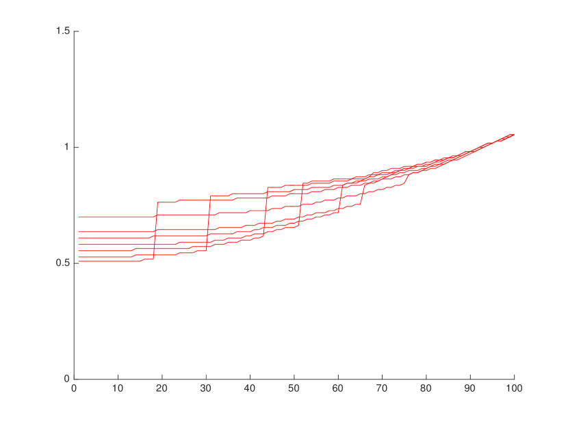
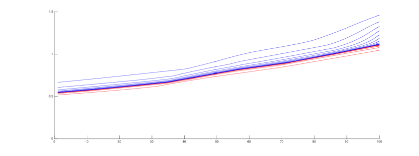
Observe that we could build the same kind of scheme to compute . We introduce this scheme because it showed better converging properties on our example than the Best Reply iterations.
We display in figure 1 and 2 a numerical experiment with the Best Reply iterations and the continuous time dynamic. Even when the hypotheses of Theorem 3 are not satisfied, the scheme displayed good converging properties. Our intuition is that it maintains the monotonic structure of the problem even when Tarksy’s fixed-point theorem hypotheses are not satisfied.
7. Conclusion and possible extension
We have identified a class of Bayesian games for which we showed that there exists a unique pure Nash equilibrium to which a simple dynamic converges. Numerical experiments seem to indicate that those results could be reinvestigated with weaker assumptions. Further works include the extension to general bidding functions (for instance, by replacing the constant marginal rate with a piece-wise linear one [17]).
References
- [1] Kenneth J. Arrow and Leonid Hurwicz, Stability of the gradient process in n-person games, Journal of the Society for Industrial and Applied Mathematics 8 (1960), no. 2, 280–294.
- [2] Susan Athey, Single crossing properties and the existence of pure strategy equilibria in games of incomplete information, Econometrica 69 (2001), no. 4, 861–889.
- [3] Péter Bayer, György Kozics, and Nóra Gabriella Szőke, Best-response dynamics in directed network games, arXiv preprint arXiv:2101.03863 (2021).
- [4] Ulrich Berger, Learning in games with strategic complementarities revisited, Journal of Economic Theory 143 (2008), no. 1, 292–301.
- [5] Ulrich Berger et al., The convergence of fictitious play in games with strategic complementarities: A comment, MPRA Paper (2009), no. 20241.
- [6] George W Brown, Some notes on computation of games solutions, Tech. report, DTIC Document, 1949.
- [7] Maria Carmela Ceparano and Federico Quartieri, Nash equilibrium uniqueness in nice games with isotone best replies, Journal of Mathematical Economics 70 (2017), 154–165.
- [8] Larry A Chenault, On the uniqueness of nash equilibria, Economics Letters 20 (1986), no. 3, 203–205.
- [9] Aaron S Edlin and Chris Shannon, Strict monotonicity in comparative statics, Journal of Economic Theory 81 (1998), no. 1, 201–219.
- [10] Gadi Fibich and Arieh Gavious, Asymmetric first-price auctions—a perturbation approach, Mathematics of operations research 28 (2003), no. 4, 836–852.
- [11] Gadi Fibich and Nir Gavish, Numerical simulations of asymmetric first-price auctions, Games and Economic Behavior 73 (2011), 479–495.
- [12] Daniel Gabay, On the uniqueness and stability of nash-equilibria in noncooperative games, Applied Stochastic Control in Economatrics and Management Science (1980).
- [13] Gerard Gaudet and Stephen W Salant, Uniqueness of cournot equilibrium: new results from old methods, The Review of Economic Studies 58 (1991), no. 2, 399–404.
- [14] Wayne Roy Gayle and Jean Francois Richard, Numerical solutions of asymmetric, first-price, independent private values auctions, Computational Economics 32 (2008), 245–278.
- [15] J. Goodman, Note on existence and uniqueness of equilibrium points for concave n-person games, Econometrica 48 (1965), 251–251.
- [16] Benjamin Heymann and Alejandro Jofré, Cost-minimizing regulations for a wholesale electricity market, (2015).
- [17] by same author, Mechanism design and allocation algorithms for network markets with piece-wise linear costs and externalities, working paper or preprint, December 2016.
- [18] Bernard Lebrun, First price auctions in the asymmetric n bidder case, International Economic Review 40 (1999), no. 1, 125–142.
- [19] Robert C Marshall, Michael J Meurer, Jean-Francois Richard, and Walter Stromquist, Numerical analysis of asymmetric first price auctions, Games and Economic behavior 7 (1994), no. 2, 193–220.
- [20] Eric Maskin, John Riley, et al., Uniqueness of equilibrium in sealed high-bid auctions, Games and Economic Behavior 45 (2003), no. 2, 395–409.
- [21] David McAdams, Isotone equilibrium in games of incomplete information, Econometrica 71 (2003), no. 4, 1191–1214.
- [22] Paul Milgrom and John Roberts, Rationalizability, learning, and equilibrium in games with strategic complementarities, Econometrica: Journal of the Econometric Society (1990), 1255–1277.
- [23] by same author, Adaptive and sophisticated learning in normal form games, Games and economic Behavior 3 (1991), no. 1, 82–100.
- [24] by same author, Comparing equilibria, The American Economic Review (1994), 441–459.
- [25] Paul R Milgrom and Robert J Weber, A theory of auctions and competitive bidding, Econometrica: Journal of the Econometric Society (1982), 1089–1122.
- [26] Philip J Reny, On the existence of monotone pure-strategy equilibria in bayesian games, Econometrica 79 (2011), no. 2, 499–553.
- [27] Philip J Reny and Shmuel Zamir, On the existence of pure strategy monotone equilibria in asymmetric first-price auctions, Econometrica 72 (2004), no. 4, 1105–1125.
- [28] Julia Robinson, An iterative method of solving a game, Annals of Mathematics 54 (1951), no. 2, 296–301.
- [29] J Ben Rosen, Existence and uniqueness of equilibrium points for concave n-person games, Econometrica: Journal of the Econometric Society (1965), 520–534.
- [30] Chris Shannon, Weak and strong monotone comparative statics, Economic Theory 5 (1995), no. 2, 209–227.
- [31] Alfred Tarski et al., A lattice-theoretical fixpoint theorem and its applications., Pacific journal of Mathematics 5 (1955), no. 2, 285–309.
- [32] Donald M Topkis, Minimizing a submodular function on a lattice, Operations research 26 (1978), no. 2, 305–321.
- [33] by same author, Supermodularity and complementarity, Princeton university press, 1998.
- [34] Timothy Van Zandt and Xavier Vives, Monotone equilibria in bayesian games of strategic complementarities, Journal of Economic Theory 134 (2007), no. 1, 339–360.
- [35] Xavier Vives, Nash equilibrium with strategic complementarities, Journal of Mathematical Economics 19 (1990), no. 3, 305–321.
- [36] by same author, Complementarities and games: New developments, Journal of Economic Literature 43 (2005), no. 2, 437–479.