Semiparametric Bernstein-von Mises for a Parameter in the Heat Equation

Abstract

We consider a Bayesian approach for the recovery of the thermal diffusivity for the heat equation when the initial temperature map of the system is unknown. This is a semiparametric inverse problem as the diffusivity is a one-dimensional parameter while the initial condition is infinite-dimensional. We assume that we have access to noisy observations of the system at the initial time $0$ and a final time $T$. We put a Gaussian process prior on the initial condition, and prove a Bernstein-von Mises (BvM) theorem for the marginal posterior of the thermal diffusivity provided that the prior regularity satisfies a restriction determined by the smoothness of the initial condition. We also investigate the behaviour of the marginal posterior for different prior regularities numerically, indicating that the BvM result is not valid if the prior regularity does not satisfy the restriction.

1 Introduction

In nonparametric statistical inverse problems the goal is to recover a function $f$ from a noisy observation of a transformed version $K\!f$ of the function, where $K$ is some known operator, typically with unbounded inverse. Many methods have been proposed and studied for this problem, including frequentist regularization methods and nonparametric Bayes approaches. The focus in the theoretical literature is mostly on the setting that the operator $K$ is known and the function $f$ is the unknown object of interest that needs to be recovered from the data. In several important applications however, the operator $K=K_{\theta}$ depends on an unknown, Euclidean parameter $\theta$, and it is that parameter which is actually the main object of interest.

An example from biology occurs in the paper [9], which deals with the modelling of biochemical interaction networks. In that case $K=K_{\theta}$ is the solution operator of a linear ordinary differential equation describing the time evolution of gene expression levels. The function $f$ describes how the activity of a so-called transcription factor changes over time and the parameter vector $\theta$ describes important aspects of the chemical reaction that is modelled, like the basal transcription rate and the rate of decay of mRNA. Another setting in which problems of this type arise naturally is in cosmology. In general relativity for instance, Einstein’s equations describe how the large-scale structure of the universe evolves from small energy density fluctuations in the early universe. These equations are partial differential equations that depend on a number of important cosmological constants that cosmologists want to learn. Given the early state $f$ of the universe, general relativity gives “forward” predictions $K_{\theta}f$ of certain observable quantities. By comparing these predictions with (noisy) observations, inference can be made about the parameters $\theta$. In such applications the operator $K_{\theta}$ is typically an operator giving an appropriate solution to Einstein’s equations. A particular example of this approach occurs in weak lensing, which is the state-of-the-art method used in recent and future cosmological surveys, see for instance [8]. In that case the parameter vector $\theta$ of interest includes important constants like the matter density of the universe and the matter inhomogeneity.

The natural Bayesian approach to this type of statistical inverse problems with parameter-dependent operators, often followed in practice, starts with endowing the pair $(\theta,f)$ with a prior distribution. The particular data generating mechanism gives rise to a likelihood and together the prior and the likelihood yield a posterior distribution for the unknown pair $(\theta,f)$. The marginal posterior for $\theta$ can then be used to make inference about $\theta$. This paper is motivated by the fact that this type of Bayesian methodology is commonly used in inverse problems with parameter-dependent operators, yet there are no readily applicable theoretical results giving insight into their fundamental performance.

To obtain some first insight we study these matters in this paper in the context of a semiparametric inverse problem that is interesting yet relatively tractable mathematically. We consider the one-dimensional heat equation which describes the evolution of the temperature in a thin metal rod as a function of position and time. The dynamics of the system up to a final time $T>0$ are governed by the partial differential equation

$${\frac{\partial}{\partial t}}u(x,t)=\theta\frac{\partial^{2}}{\partial x^{2}}u(x,t),\text{ \text{ }}u(x,0)=f(x),\text{ \text{ }}u(0,t)=u(1,t)=0,$$ (1)

where $u$ defined on $[0,1]\times[0,T]$ is the temperature function and $f\in L^{2}[0,1]$ represents the initial condition of the temperature in the system, which is assumed to satisfy the same boundary conditions $f(0)=f(1)=0$. The parameter $\theta>0$ is the thermal diffusivity constant of the metal and is our main object of interest.

If $\theta$ is known, then inferring the initial function $f$ from noisy observations of the function $u(\cdot,T)$ at the final time $T$ is a well-known statistical inverse problem, see for instance [1], [4, 5], [11], [14], [15], [16], [18]. It is a severely ill-posed problem, since the solution operator that maps $f$ to $u(\cdot,T)$ takes functions in $L^{2}[0,1]$ to super smooth functions. Indeed, if we denote by $f_{k}$ the coefficients of $f$ with respect to the sine basis functions $e_{k}(x)=\sqrt{2}\sin(k\pi x)$, then the solution of (1) can be expressed as

$$u(x,t)=\sqrt{2}\sum_{k=1}^{\infty}f_{k}e^{-\theta\pi^{2}tk^{2}}\sin(k\pi x).$$ (2)

As a consequence, the optimal, minimax rate for estimators that recover $f$ from a noisy observation of $u(0,T)$ is known to be of the order $(\log n)^{-\beta/2}$ (with respect to $L^{2}$-loss), where $\beta$ is the (Sobolev) regularity of $f$ and $n$ is the signal-to-noise ratio, or sample size. Various frequentist and Bayesian methods achieve this rate, see for instance [15, 16, 11, 1, 14].

In this paper our interest is not in recovering the initial temperature distribution $f$ however, but rather in learning the diffusivity parameter $\theta$ from data, while still assuming that $f$ is unknown as well. Just observing the solution of the equation at final time $T$ is then not sufficient to identify the parameter $\theta$, as can be seen from (2). Instead we assume that we have noisy observations of the system (1) at times $0$ and $T$. More precisely, if we denote by $K_{\theta}:L^{2}[0,1]\to L^{2}[0,1]$ the solution operator

$$K_{\theta}f=\sum_{k=1}^{\infty}\langle f,e_{k}\rangle e^{-\theta\pi^{2}Tk^{2}}e_{k},$$ (3)

we assume that we have observations $X^{(1)}=(X^{(1)}_{t}:t\in[0,1])$ and
$X^{(2)}=(X^{(2)}_{t}:t\in[0,1])$ satisfying

$$dX^{(1)}_{t} =f(t)\,dt+\frac{1}{\sqrt{n}}\,dW^{(1)}_{t},$$ (4)

$$dX^{(2)}_{t} =K_{\theta}f(t)\,dt+\frac{1}{\sqrt{n}}\,dW^{(2)}_{t},$$ (5)

where $W^{(1)}$ and $W^{(2)}$ are independent Brownian motions and $n$ is the signal-to-noise ratio (Expanding in the basis $e_{k}$ shows that this is equivalent to observing noisy versions of the coefficients of $f$ and $u(\cdot,T)$ relative to the basis $e_{k}$). We take a Bayesian approach and endow the pair $(\theta,f)$ with a prior distribution by putting a Gaussian process prior on $f$ and an independent prior with a positive, continuous Lebesgue density on $\theta$. We present results that describe the behaviour of the marginal posterior for the parameter $\theta$ of interest as $n\to\infty$.

Our main result is Theorem 2.1, a semiparametric Bernstein-von Mises (BvM) theorem for the marginal posterior of $\theta$ when putting a Gaussian process prior on $f$. It gives conditions under which the marginal posterior behaves asymptotically like a normal distribution centered at an efficient estimator of $\theta$, with a variance equal to the inverse of the efficient Fisher information. Such a result guarantees in particular validity of uncertainty quantification, in the sense that that credible intervals for the parameter $\theta$ obtained from the marginal posterior are also asymptotic frequentist confidence intervals in that case, see for instance [2]. As the examples provided in Section 3 show, the essential condition for BvM to hold is that the regularity of the prior on $f$ is not much greater than the regularity of the true underlying $f$. We complement this in Section 4 with numerical experiments. These confirm our theoretical results and indicate that if the prior on $f$ is too smooth relative to the underlying truth then the posterior is biased, leading to unreliable inference about the parameter $\theta$.

We restrict our analysis to the particular problem (1)–(5) in this first paper on this topic, but there are certainly more general underlying mechanisms and hence potential for generalization and extension. Investigation of our proofs shows that part of the arguments would go through for other operators $K_{\theta}$ as well without many changes. On the other hand, the dependence of $K_{\theta}$ on $\theta$ plays a crucial role and results like Lemma 5.1 ahead will have to be derived separately for each particular operator $K_{\theta}$. For other examples this may be much more challenging.

We present the semiparametric setting and our main Theorem 2.1 in Section 2 and give examples of Gaussian process priors for which it can be applied in Section 3. In Section 4, we experimentally assess the result of the theorem by providing a Metropolis Hastings algorithm for sampling from an approximation of the marginal posterior for $\theta$. The proof of Theorem 2.1 is given in Section 5.

1.1 Notation

On the interval $[0,1]$, the space of square integrable functions is denoted by $L^{2}[0,1]$ and the space of Hölder continuous functions of order $\alpha$ by $C^{\alpha}[0,1]$. For functions $f,g\in L^{2}[0,1]$, $\|f\|^{2}:=\int_{0}^{1}f(x)^{2}\text{d}x$ is the $L^{2}$ norm of $f$ and $\langle f,g\rangle=\int_{0}^{1}f(x)g(x)\text{d}x$ is the $L^{2}$ inner product of $f$ and $g$. Note that when writing $\|A\|$ for an operator $A$, no confusion is possible and we naturally mean the operator norm of $A$. For two numbers $a$ and $b$, we denote by $a\wedge b$ the minimum of $a$ and $b$. Similarly $a\vee b$ denotes the maximum of $a$ and $b$. For two sequences $a_{n}$ and $b_{n}$, we mean by $a_{n}\asymp b_{n}$ that $|a_{n}/b_{n}|$ is bounded away from zero and infinity as $n\to\infty$. By $a_{n}\lesssim b_{n}$, we mean that $a_{n}/b_{n}$ is bounded. For two probability measures $P$ and $Q$ defined on the same probability space $(\Omega,\mathcal{F}),\|P-Q\|_{\text{TV}}$ is the total variational distance between $P$ and $Q$ defined by $\|P-Q\|_{\text{TV}}:=2\sup_{F\in\mathcal{F}}|P(A)-Q(A)|$. Finally, for a metric space $(A,d)$ and $\varepsilon>0$ we denote by $N(\varepsilon,A,d)$ the minimum number of balls of radius $\varepsilon$ needed to cover $A$.

2 General result

We assume that the pair $(\theta,f)$ belongs to $\Theta\times L^{2}[0,1]$, where $\Theta=(a,b)$ for some $0<a<b<\infty$. We endow the unknown pair with a prior $\Pi$ of the form $\Pi=\pi_{\theta}\times\pi_{f}$, where $\pi_{\theta}$ has a continuous Lebesgue density that is bounded away from $0$ and $\infty$ on $\Theta$ and $\pi_{f}$ is a centered Gaussian process prior on $L^{2}[0,1]$, that is, the law of a centered Gaussian process with sample paths that belong to $L^{2}[0,1]$. Girsanov’s theorem (see for instance [13]) gives an expression for the likelihood,

$$\log\frac{dP_{\theta,f}}{dP_{0}}=n\int_{0}^{1}f(t)\,dX^{(1)}_{t}+n\int_{0}^{1}K_{\theta}f(t)\,dX^{(2)}_{t}-\frac{n}{2}\|f\|^{2}-\frac{n}{2}\|K_{\theta}f\|^{2},$$

where $P_{\theta,f}$ is the law of the pair $(X^{(1)},X^{(2)})$ defined by (4)–(5) and the dominating measure $P_{0}$ is the law of $n^{-1/2}(W^{(1)},W^{(2)})$. Combined with the prior this results in a posterior distribution $\Pi(\cdot\,|\,X)$ for the pair $(\theta,f)$. Here we denote by $X=(X^{(1)},X^{(2)})$ all available data. We are in particular interested in the marginal posterior $B\mapsto\Pi(\theta\in B\,|\,X)$ of the thermal diffusivity parameter.

Since we have a real-valued parameter $\theta$ of interest and an infinite-dimensional nuisance parameter $f$, the behaviour of this marginal posterior is determined by the semiparametric structure of the model. In many texts semiparametric concepts are mainly treated in the context of i.i.d. models, see for instance [20], but of course they can be extended to non-i.i.d. models, including the one we study in this paper. The paper [17] considers a quite general setting for instance. In Section 5 ahead we show that our model fits into the semiparametric framework of [2].

To describe our semiparametric Bernstein-von Mises theorem with as little technicalities as possible, we first recall that if $f$ is known (so that we only have to consider the observations $X^{(2)}$), the model is called differentiable in quadratic mean at $\theta$ if there exists a $g_{\theta}$ such that

$$\frac{K_{\theta+h}f-K_{\theta}f}{h}\to g_{\theta}$$

in $L^{2}[0,1]$ as $h\to 0$, and that we then have local asymptotic normality (LAN) (see [12]). We note that this is the case in our model with $g_{\theta}=\dot{K}_{\theta}f$ if we define $\dot{K}_{\theta}:L^{2}[0,1]\to L^{2}[0,1]$ by

$$\dot{K}_{\theta}f=-\pi^{2}T\sum_{k=1}^{\infty}\langle f,e_{k}\rangle k^{2}e^{-\theta\pi^{2}Tk^{2}}e_{k}.$$ (6)

The notation is meant to indicate that $\dot{K}_{\theta}$ is simply the derivative of $K_{\theta}$ with respect to $\theta$. The Fisher information at $\theta$ in the model with known $f$ is then given by $I_{\theta}=\|\dot{K}_{\theta}f\|^{2}$.

To understand what happens in the semiparametric case that $f$ is unknown, consider a one-dimensional submodel of the form $t\mapsto(\theta+t/\sqrt{n},f+tg/\sqrt{n})$, for $g\in L^{2}[0,1]$. Then realizing that

$$\frac{K_{\theta+ah}(f+hg)-K_{\theta}f}{h}\to a\dot{K}_{\theta}f+K_{\theta}g$$

in $L^{2}[0,1]$ as $h\to 0$ we see using Girsanov’s theorem that for the submodel we have the LAN expansion

$$\begin{split}\log\frac{dP_{\theta+t/\sqrt{n},f+tg/\sqrt{n}}}{dP_{\theta,f}}&=t\int g\,dW^{(1)}+t\int(\dot{K}_{\theta}f+K_{\theta}g)\,dW^{(2)}\\ &\quad-\frac{1}{2}t^{2}\|g\|^{2}-\frac{1}{2}t^{2}\|\dot{K}_{\theta}f+K_{\theta}g\|^{2}+o_{P_{\theta,f}}(1)\end{split}$$ (7)

as $n\to\infty$, with $W^{(1)}$ and $W^{(2)}$ independent $P_{\theta,f}$-Brownian motions. Hence, the Fisher information in the submodel at $t=0$ is given by $\|g\|^{2}+\|\dot{K}_{\theta}f+K_{\theta}g\|^{2}$. Using the fact that $K_{\theta}$ is self-adjoint it is not hard to see that this is minimal for $g=-\gamma$, where

$$\gamma=\gamma_{\theta,f}=(I+K^{2}_{\theta})^{-1}K_{\theta}\dot{K}_{\theta}f.$$

We therefore call $\gamma$ the least favourable direction in our model. The Fisher information at $t=0$ in the least favourable submodel is given by

$$\tilde{I}_{\theta,f}=\|\dot{K}_{\theta}f\|^{2}-\langle K_{\theta}\dot{K}_{\theta}f,(I+K^{2}_{\theta})^{-1}K_{\theta}\dot{K}_{\theta}f\rangle.$$

The latter quantity is then the efficient Fisher information at $(\theta,f)$. Note that it is strictly positive and strictly smaller than the parametric Fisher information if $f\not=0$, so there is loss of information due to the fact that $f$ is unknown.

Our main general result asserts that the semiparametric BvM theorem holds for the marginal posterior distribution of the parameter $\theta$ if $\pi_{f}$ is a “good enough” Gaussian prior on the function $f$. Here “good enough” means that if $\pi_{f}$ is used as a prior to make inference about $f$ in the model (4), then the corresponding posterior contracts around the true $f_{0}$ (with respect to the $L^{2}$-norm) at a rate $\varepsilon_{n}$ that is of smaller order than $n^{-1/4}$. We recall that the rate $\varepsilon_{n}$ is determined by the so-called the concentration function $\varphi_{f_{0}}$ associated to the centered Gaussian prior $\pi_{f}$ on $L^{2}[0,1]$, which is defined by

$$\varphi_{f_{0}}(\varepsilon)=\inf_{h\in\mathbb{H}:\|h-f_{0}\|\leq\varepsilon}\|h\|^{2}_{\mathbb{H}}-\log\pi_{f}(f:\|f\|\leq\varepsilon),$$

where $\mathbb{H}$ is the reproducing kernel Hilbert space (RKHS) of $\pi_{f}$ (see [21]). If $f_{0}$ is the true function in the model (4) and $\varepsilon_{n}$ is a sequence of positive numbers such that $n\varepsilon^{2}_{n}\to\infty$ and the concentration inequality $\varphi_{f_{0}}(\varepsilon_{n})\leq n\varepsilon^{2}_{n}$ holds, then the posterior corresponding to the prior $\pi_{f}$ contracts around $f_{0}$ with respect to the $L^{2}$-norm at the rate $\varepsilon_{n}$ (see Theorem 3.4 of [22]).

The theorem below says that semiparametric Bernstein-von Mises holds for the marginal posterior of $\theta$ if the concentration inequality $\varphi_{f_{0}}(\varepsilon_{n})\leq n\varepsilon^{2}_{n}$ holds for a rate $\varepsilon_{n}$ that is of smaller order than $n^{-1/4}$ and, in addition, the least favourable direction $\gamma_{\theta_{0},f_{0}}$ can be approximated by elements of the RKHS of $\pi_{f}$ in the same way as the true function $f_{0}$. The latter condition is expressed by imposing that the concentration inequality holds for $\gamma_{\theta_{0},f_{0}}$ as well, that is, we also have $\varphi_{\gamma_{\theta_{0},f_{0}}}(\varepsilon_{n})\leq n\varepsilon^{2}_{n}$. In principle the statement of the theorem can be extended to allow for approximation of $\gamma_{\theta_{0},f_{0}}$ at a slower rate $\rho_{n}$, adding the condition that $\sqrt{n}\varepsilon_{n}\rho_{n}\to 0$. However, as we will discuss in the next section, the mapping properties of the solution operator $K_{\theta_{0}}$ imply that $\gamma_{\theta_{0},f_{0}}$ is very smooth, and in particular smoother than the true function $f_{0}$. This means that the condition on the least favourable direction as phrased in the theorem is automatically fulfilled for many Gaussian process priors with a rich enough RKHS. In fact, we will see that for many priors we have that $\gamma_{\theta_{0},f_{0}}$ actually belongs to the RKHS itself, so that the condition is trivially satisfied. What remains is the condition $n\varepsilon_{n}^{4}\to 0$, which typically gives a restriction on the relation between the regularity of the true $f_{0}$ and the regularity of the prior $\pi_{f}$, as we will illustrate in the examples in Section 3.

Recall that by $\|\cdot\|_{\text{TV}}$ we denote the total variation distance between probability measures. We denote the true parameter pair by $(\theta_{0},f_{0})$.

Theorem 2.1.

Let $f_{0}\not=0$ and suppose there exists a sequence $\varepsilon_{n}\downarrow 0$ such that $n\varepsilon^{2}_{n}\gtrsim\log n$ and $n\varepsilon^{4}_{n}\to 0$ and we have the concentration inequalities $\varphi_{f_{0}}(\varepsilon_{n})\leq n\varepsilon^{2}_{n}$ and $\varphi_{\gamma_{\theta_{0},f_{0}}}(\varepsilon_{n})\leq n\varepsilon^{2}_{n}$. Then

$$\Big{\|}\Pi(\theta\in\cdot\,|\,X)-N\Big{(}\theta_{0}+\frac{1}{\sqrt{n}}\Delta_{\theta_{0},f_{0}},\frac{1}{n}\tilde{I}^{-1}_{\theta_{0},f_{0}}\Big{)}\Big{\|}_{\text{TV}}\to 0$$

in $P_{\theta_{0},f_{0}}$-probability as $n\to\infty$, where $\Delta_{\theta_{0},f_{0}}\sim N(0,\tilde{I}^{-1}_{\theta_{0},f_{0}})$.

The proof of the theorem is given in Section 5. In the next section we first investigate what the result looks like for a number of concrete Gaussian process priors $\pi_{f}$.

3 Results for specific Gaussian process priors

In this section we consider various natural and commonly used choices of Gaussian process priors $\pi_{f}$. These priors all have a hyperparameter than can be viewed as describing a form of “smoothness”, or “regularity” of the prior. We investigate in particular for which combinations of prior regularity and regularity of the true function $f_{0}$ we have that the Bernstein-von Mises result of Theorem 2.1 holds.

To verify the condition involving the least favourable direction we note that by the explicit expressions for the operators $K_{\theta}$ and $\dot{K}_{\theta}$ it is given by

$$\gamma_{\theta_{0},f_{0}}=-\pi^{2}T\sum_{k=1}^{\infty}\frac{k^{2}\langle f_{0},e_{k}\rangle e^{-2\theta_{0}\pi^{2}Tk^{2}}}{1+e^{-2\theta_{0}\pi^{2}Tk^{2}}}e_{k}.$$

The fact that the coefficients of $\gamma_{\theta_{0},f_{0}}$ with respect to the sine basis functions $e_{k}$ are decreasing exponentially fast implies that the function is very smooth in various senses. It is for instance infinitely often continuously differentiable. As a result $\gamma_{\theta_{0},f_{0}}$ belongs to the RKHS of many Gaussian process priors that are natural choices for $\pi_{f}$ in the present setting.

Example 3.1 (Series prior).

Since the operator $K_{\theta}$ diagonalizes on the sine basis $e_{k}$, it is natural to consider a prior on $f$ with a covariance that diagonalizes on this basis as well. In this example we therefore consider the prior $\pi_{f}$ defined as the distribution of the random series

$$W=\sum_{k=1}^{\infty}\sigma_{k}Z_{k}e_{k},$$

where the $e_{k}$ are the sine basis functions introduced above, the $Z_{k}$ are independent standard normal variables and $\sigma_{k}$ is a sequence of standard deviations that satisfies $\sum\sigma^{2}_{k}<\infty$, ensuring that the random series defines a random element in $L^{2}[0,1]$. We will in particular consider the choice $\sigma_{k}\asymp k^{-1/2-\alpha}$ for $\alpha>0$. This yields a prior on $f$ which (almost) has regularity $\alpha$ in Sobolev-type sense with respect to the sine basis. Indeed, for all $s<\alpha$ we have that $\sum k^{2s}\langle W,e_{k}\rangle^{2}<\infty$ almost surely. We assume that $f_{0}$ has regularity $\beta$ in the same sense, that is, $\|f_{0}\|^{2}_{\beta}=\sum k^{2\beta}\langle f_{0},e_{k}\rangle^{2}<\infty$. (We note that since we consider the sine basis here, this notion of regularity is closely related to, but not exactly the same as the usual Sobolev regularity.)

Let $\mathbb{H}$ be the reproducing kernel Hilbert space of the process $W$. According to Theorem 4.2 of [21] it is given by

$$\mathbb{H}=\Big{\{}h=\sum c_{k}e_{k}:\|h\|^{2}_{\mathbb{H}}=\sum\frac{c^{2}_{k}}{\sigma^{2}_{k}}<\infty\Big{\}}.$$

By Corollary 4.3 of [7] we have that $-\log\pi_{f}(\|f\|\leq\varepsilon)\lesssim\varepsilon^{-1/\alpha}$. For $K\geq 1$, consider $h=\sum_{k\leq K}\langle f_{0},e_{k}\rangle e_{k}\in\mathbb{H}$. We have $\|h-f_{0}\|\leq K^{-\beta}\|f_{0}\|_{\beta}$ and $\|h\|^{2}_{\mathbb{H}}=\sum_{k\leq K}\langle f_{0},e_{k}\rangle^{2}/\sigma^{2}_{k}\lesssim(1\vee K^{1+2(\alpha-\beta)})\|f_{0}\|^{2}_{\beta}$. Given $\varepsilon>0$ we take $K\asymp(\|f_{0}\|_{\beta}/\varepsilon)^{1/\beta}$ to find that

$$\varphi_{f_{0}}(\varepsilon)\lesssim(\varepsilon^{-\frac{1+2(\alpha-\beta)}{\beta}}\vee 1)+\varepsilon^{-\frac{1}{\alpha}}.$$

It follows that for $\varepsilon_{n}=cn^{-\alpha\wedge\beta/(1+2\alpha)}$, with $c>0$ large enough, we have the inequality $\varphi_{f_{0}}(\varepsilon_{n})\leq n\varepsilon^{2}_{n}$.

We clearly have $n\varepsilon^{2}_{n}\gtrsim\log n$ and the condition $n\varepsilon^{4}_{n}\to 0$ translates into the requirement that $1/2<\alpha<2\beta-1/2$. The fact that the coefficients of $\gamma_{\theta_{0},f_{0}}$ with respect to the sine basis decay exponentially fast implies that $\gamma_{\theta_{0},f_{0}}\in\mathbb{H}$, irrespective of the values of $\alpha$ and $\beta$. Hence, the condition on $\gamma_{\theta_{0},f_{0}}$ is trivially satisfied. We conclude that the Bernstein-von Mises result holds in this case if $1/2<\alpha<2\beta-1/2$.

The next examples show that it is in fact not necessary to use a prior on $f$ that is compatible with the operator $K_{\theta}$ as in the preceding case. Commonly used Gaussian process priors work just as well and give similar results. Only the appropriate type of regularity to describe the result is slightly different in each case.

Example 3.2 (Integrated Brownian motion).

Define the $k$-fold integration operators $I_{0+}^{k}$ by $I_{0+}^{0}f=f$ and $I^{k}_{0+}f(t)=\int_{0}^{t}I^{k-1}_{0+}f(s)\,ds$ for $k\in\mathbb{N}$. Now fix $k\in\mathbb{N}_{0}$ and let $\pi_{f}$ be the law of the centered Gaussian process

$$W_{t}=\sum_{i=0}^{k}t^{i}Z_{i}+I_{0+}^{k}B(t),\qquad t\in[0,1],$$

where $Z_{0},\ldots,Z_{k}$ are independent standard normal variables and $B$ is a standard Brownian motion independent of the $Z_{i}$. (The independent polynomial is added to the $k$-fold integrated Brownian motion because the process itself and its $k$ derivatives would otherwise all vanish at $0$, which is undesirable.) The well-known properties of Brownian motion imply that the process $W$ (almost) has regularity $\alpha=k+1/2$, in the sense that its sample paths almost surely belong to $C^{s}[0,1]$ for every $s<\alpha$. We assume that $f_{0}\in C^{\beta}[0,1]$ for $\beta>0$.

It is known that in this situation the concentration inequality $\varphi_{f_{0}}(\varepsilon)\leq n\varepsilon^{2}_{n}$ holds again for $\varepsilon_{n}=cn^{-\alpha\wedge\beta/(1+2\alpha)}$, with $c>0$ large enough, see Section 11.4.1 of [10]. The RKHS of $W$ is the (usual) $L^{2}$-Sobolev space of regularity $\alpha+1/2=k+1$, consisting of the functions on $[0,1]$ that are $k$ times differentiable, and with $k$th derivative $f^{(k)}$ that is absolutely continuous with derivative $f^{(k+1)}$ in $L^{2}[0,1]$ (see Lemma 11.29 of [10]). Hence, since $\gamma_{\theta_{0},f_{0}}$ is infinitely often continuously differentiable it belongs to this RKHS and the condition on $\gamma_{\theta_{0},f_{0}}$ is trivially satisfied again. We conclude that also in this case we have that the Bernstein-von Mises result holds if $1/2<\alpha<2\beta-1/2$.

It is straightforward to extend this example from multiply integrated Brownian motion to the more general Riemann-Liouville process, which also covers fractional integrals of Brownian motion. See Section 11.4.2 of [10].

Example 3.3 (Matérn process).

In this example we let $\pi_{f}$ be the law of a (one-dimensional) Matérn process with parameter $\alpha>0$. This is a centered, stationary Gaussian process $W$ with spectral measure $\mu_{\alpha}(d\lambda)=(1+\lambda^{2})^{-1/2-\alpha}d\lambda$, that is,

$$\mathbb{E}W_{s}W_{t}=\int_{\mathbb{R}}\frac{e^{i\lambda(t-s)}}{(1+\lambda^{2})^{1/2+\alpha}}\,d\lambda.$$

(The stationary Ornstein-Uhlenbeck process is a particular example, corresponding to $\alpha=1/2$.) It can be shown that the sample paths of the Matérn process almost surely belong to $C^{s}[0,1]$ for all $s<\alpha$. We assume that for $\beta>0$ we have $f_{0}\in C^{\beta}[0,1]\cap H^{\beta}[0,1]$, where $H^{\beta}[0,1]$ is the Sobolev space defined as the space of restrictions to $[0,1]$ of functions $f\in L^{2}(\mathbb{R})$ with Fourier transform $\hat{f}$ that satisfies $\int(1+\lambda^{2})^{\beta}|\hat{f}(\lambda)|^{2}\,d\lambda<\infty$.

By Lemmas 11.36 and 11.37 of [10] we have $\varphi_{f_{0}}(\varepsilon_{n})\leq n\varepsilon^{2}_{n}$ for $\varepsilon_{n}=cn^{-\alpha\wedge\beta/(1+2\alpha)}$, with $c>0$ large enough. The RKHS of $W$ is the space of (restrictions to $[0,1]$ of) real parts of functions $h$ that can be written as $h(t)=\int e^{i\lambda t}\psi(\lambda)\mu_{\alpha}(d\lambda)$ for some $\psi\in L^{2}(\mu_{\alpha})$, see Lemma 11.35 of [10]. The smoothness on $[0,1]$ implies that $\gamma_{\theta_{0},f_{0}}$ can be extended to a compactly supported $C^{\infty}$-function on the whole line. The Fourier transform $\hat{\gamma}_{\theta_{0},f_{0}}$ of this extension then has the property that $|\lambda|^{p}|\hat{\gamma}_{\theta_{0},f_{0}}(\lambda)|\to 0$ for every $p>0$ as $|\lambda|\to\infty$. By Fourier inversion the extended function can be written as

$$\gamma_{\theta_{0},f_{0}}(t)=\int e^{i\lambda t}\hat{\gamma}_{\theta_{0},f_{0}}(\lambda)\,d\lambda=\int e^{i\lambda t}\psi(\lambda)\mu_{\alpha}(d\lambda),$$

where $\psi(\lambda)=(1+\lambda^{2})^{1/2+\alpha}\hat{\gamma}_{\theta_{0},f_{0}}(\lambda)$. By the observation just made about the tails of $\hat{\gamma}_{\theta_{0},f_{0}}$ we have that $\psi\in L^{2}(\mu_{\alpha})$, hence $\gamma_{\theta_{0},f_{0}}$ belongs to the RKHS of $W$. So as in the preceding examples we have that the condition on $\gamma_{\theta_{0},f_{0}}$ is trivially satisfied and the Bernstein-von Mises result holds if $1/2<\alpha<2\beta-1/2$.

The least favourable direction generally does not belong to the RKHS of the squared exponential process. It can can be suitably approximated by elements of the RKHS of this prior however, so the Bernstein-von Mises result also holds if the (rescaled) squared exponential is used as prior on $f$. We note that in this example the prior depends on the signal-to-noise ratio $n$ through the length scale of the Gaussian process. Although it is not made explicit in the statement of Theorem 2.1, inspection of the proofs shows that it remains valid for $n$-dependent priors.

Example 3.4 (Squared exponential process).

Let $\pi_{f}$ be the law of the squared exponential process $W$ with length scale $l=l_{n,\alpha}=n^{-1/(1+2\alpha)}$ for $\alpha>0$, so

$$\mathbb{E}W_{s}W_{t}=e^{-(t-s)^{2}/l^{2}}.$$

The sample paths of the squared exponential process are analytic functions, but still in view of the results of [19] it makes sense to think of the rescaled process $W$ as “essentially” having regularity $\alpha$. We assume that $f_{0}\in C^{\beta}[0,1]$ for $\beta>0$.

By Lemma 2.2 and Theorem 2.4 of [19] the inequality $\varphi_{f_{0}}(\varepsilon_{n})\leq n\varepsilon^{2}_{n}$ holds in this case for $\varepsilon_{n}=cn^{-\alpha\wedge\beta/(1+2\alpha)}\log n$, with $c>0$ large enough. Note that also in this case we have $n\varepsilon_{n}^{4}\to 0$ if and only if $1/2<\alpha<2\beta-1/2$, the extra logarithmic factor in the rate $\varepsilon_{n}$ has no influence on this condition.

The spectral measure of the stationary process $W$ is given by $\mu(d\lambda)=\mu_{n,\alpha}(d\lambda)=l(2\sqrt{\pi})^{-1}e^{-l^{2}\lambda^{2}/4}\,d\lambda$ and as in the preceding example the RKHS $\mathbb{H}$ of $W$ is the space of (restrictions to $[0,1]$ of) real parts of functions $h$ that can be written as $h(t)=\int e^{i\lambda t}\psi(\lambda)\mu(d\lambda)$ for some $\psi\in L^{2}(\mu)$, and the RKHS norm of such an element of $\mathbb{H}$ is given by $\|h\|_{\mathbb{H}}=\|\psi\|_{L^{2}(\mu)}$ (see Lemma 11.35 of [10]). In the preceding example we noted that $\gamma_{\theta_{0},f_{0}}$ extends to a compactly support $C^{\infty}$-function on $\mathbb{R}$ that can be written as $\gamma_{\theta_{0},f_{0}}(t)=\int e^{i\lambda t}\hat{\gamma}_{\theta_{0},f_{0}}(\lambda)\,d\lambda$, where the Fourier transform $\hat{\gamma}_{\theta_{0},f_{0}}(\lambda)$ has tails that decay faster than any polynomial. Now for $K>0$, let

$$h(t)=\int_{-K}^{K}e^{i\lambda t}\hat{\gamma}_{\theta_{0},f_{0}}(\lambda)\,d\lambda.$$

Then for every $p>0$ we have $\|h-\gamma_{\theta_{0},f_{0}}\|^{2}\lesssim\int 1_{|\lambda|>K}|\lambda|^{-1-2p}\,d\lambda\lesssim K^{-2p}$. Moreover we have $h(t)=\int e^{i\lambda t}\psi(\lambda)\mu(d\lambda)$, where

$$\psi(\lambda)=\frac{2\sqrt{\pi}}{l}1_{|\lambda|\leq K}e^{\frac{l^{2}\lambda^{2}}{4}}\hat{\gamma}_{\theta_{0},f_{0}}(\lambda).$$

It follows that $\|h\|^{2}_{\mathbb{H}}=\|\psi\|^{2}_{L^{2}(\mu)}\lesssim l^{-1}e^{\frac{l^{2}K^{2}}{4}}$. Taking and $K=1/l$ and $p>\alpha\wedge\beta$ we obtain

$$\inf_{h\in\mathbb{H}:\|h-\gamma_{\theta_{0},f_{0}}\|\leq\varepsilon_{n}}\|h\|^{2}_{\mathbb{H}}\lesssim n^{1/(1+2\alpha)}\leq n\varepsilon^{2}_{n}$$

and hence, after enlarging the constant $c$ if necessary, $\varphi_{\gamma_{\theta_{0},f_{0}}}(\varepsilon_{n})\leq n\varepsilon^{2}_{n}$. So also with this prior $\pi_{f}$ the Bernstein-von Mises result holds if $1/2<\alpha<2\beta-1/2$.

In fact by the results of [19] this example generalizes to any process $W_{t/l}$, where $W$ is a centered stationary Gaussian process with a spectral measure $\mu$ that satisfies $\int e^{\delta|\lambda|}\,\mu(d\lambda)<\infty$ for some $\delta>0$.

So we see that many common choices of Gaussian process priors for $\pi_{f}$ lead to the Bernstein-von Mises result for the marginal posterior of $\theta$. Although the precise appropriate notion of smoothness differs from case to case, the condition is every time that the regularity $\alpha$ of the prior and the regularity $\beta$ of the true $f_{0}$ should satisfy the constraints $1/2<\alpha<2\beta-1/2$. In other words it is not necessary that the prior $\pi_{f}$ is tuned optimally, leading to an optimal contraction rate for the marginal posterior of $f$. It is fine if the prior is undersmoothing, and a limited degree of oversmoothing is allowed as well. This phenomenon has been observed before in several other instances of the semiparametric Bernstein-von Mises theorem, see for instance [2], [6], [3].

4 Posterior simulations

In this section, we present the results of our simulations to illustrate the application of Theorem 2.1. We begin by reformulating the model to use the series representation for the prior, which is more convenient for sampling using Monte-Carlo Markov Chain (MCMC) methods. We select a ground truth $(\theta_{0},f_{0})$ and implement a Metropolis-Hastings (MH) algorithm to sample from the marginal posterior distribution of $\theta$. We repeat this process for different prior regularities $\alpha$ and examine the resulting marginal posterior distribution of $\theta$. We also provide trace plots to assess the convergence of our algorithm.

For a given pair of parameters, the signal-in-white noise model we consider is equivalent to observing the following samples for all $k\in\mathbb{N}$:

$$X^{(1)}_{k}=f_{k}+\frac{1}{\sqrt{n}}\zeta^{1}_{k},$$

$$X^{(2)}_{k}=e^{-ck^{2}\theta}f_{k}+\frac{1}{\sqrt{n}}\zeta^{2}_{k},$$

where the $\zeta^{1}_{k}$ and $\zeta^{2}_{k}$ are i.i.d. standard Gaussians. In practice, we compute an approximation of the posterior by considering only the first $m$ observations. This yields the following expression for the approximate likelihood:

$$\ell(\theta,f\mid X)=\dfrac{n^{K}}{\sqrt{2\pi}^{2K}}\prod_{k\leq m}\exp\left(-\dfrac{n}{2}(X^{(1)}_{k}-f_{k})^{2}-\dfrac{n}{2}(X^{(2)}_{k}-e^{-ck^{2}\theta}f_{k})^{2}\right).$$ (8)

We put a uniform prior on $\theta$ and consider the prior series representation of the GP prior on $f$ already mentioned in Example 3.1.

$$\pi^{\sigma}_{f}\sim\sum_{k=1}^{\infty}\sigma_{k}\nu_{k}e_{k},$$

where the $\nu_{k}$ are i.i.d $N(0,1)$ random variables and where $\sigma_{k}=(k+1)^{-1/2-\alpha}$ where $\alpha>0$ is the chosen regularity of the prior. It follows that the prior is distributed as follows

$$(\theta,f_{1},\cdots,f_{m})\sim U(\Theta)\times\prod_{k=1}^{m}N\left(0,(k+1)^{-1-2\alpha}\right).$$

Furthermore, by integrating $\Pi(\theta,f)\ell(\theta,f|X)$ with respect to to the $f_{k}$’s, we obtain that the marginal posterior for $\theta,\Pi(\theta\mid X)$ is proportional to the following quantity:

$$\prod_{k\leq m}(n+ne^{-ck^{2}\theta}+(k+1)^{2\alpha+1})^{-1/2}\exp\left(\dfrac{(nX^{(1)}_{k}+nX^{(2)}_{k}e^{-ck^{2}\theta})^{2}}{2(n+ne^{-ck^{2}\theta}+(k+1)^{2\alpha+1})}\right).$$ (9)

Our MH algorithm will use (9) as a target distribution. For the proposal step, we sample from a normal distribution centered at the previous proposal value with standard deviation $\sigma_{\theta}$. The details of our sampling procedure are described in Algorithm 1.

Data: Observed data $\mathbf{X^{(1)},X^{(2)}}$, signal-to-noise ratio $\mathbf{n}$, regularity $\boldsymbol{\alpha}$, initial value $\boldsymbol{\theta^{(1)}}$, number of iterations $\mathbf{T}$, std.deviation for proposal distribution $\boldsymbol{\sigma_{\theta}}$.

Result: Samples from the posterior distribution.

for $t=2$ to $\mathbf{T}$ do

      

      Sample $\theta^{*}$ from $N(\theta^{(t-1)},\boldsymbol{\sigma_{\theta}}^{2})$

      Compute the acceptance ratio $A(\theta^{*},\theta^{(t-1)})=\frac{\Pi(\theta^{*}|\mathbf{X^{(1)}},\mathbf{X^{(2)}})}{\Pi(\theta^{(t-1)}|\mathbf{X^{(1)}},\mathbf{X^{(2)}})}$ using (9)

      Sample $u$ from the uniform distribution over $(0,1)$

      if $u<A(\theta^{*},\theta^{(t-1)})$ then

             $\theta^{(t)}=\theta^{*}$

       end if

      else

             $\theta^{(t)}=\theta^{(t-1)}$

       end if

      

end for

Algorithm 1 Metropolis-Hastings Algorithm

We fix $T=1$, let $\theta_{0}=0.01$ and consider the function $f_{0}$ defined as follows:

$$f_{0}(x)=\sum_{k=1}^{\infty}k^{-2}e_{k}(x).$$

We have that $f$ is Sobolev smooth of order $\beta=3/2$. Our BvM theorem is guaranteed for $0.5<\alpha<2.5$. We fix $m=100$ and generate data vectors $X^{(1)}$ and $X^{(2)}$ with signal-to-noise ratio $n=10^{5}$. We run Algorithm 1 for $10^{5}$ iterations with a burn in period of 1000. For a correctly chosen $\alpha$ in the zone ($\alpha=1$), we run Algorithm 1 on different datasets and observe that the marginal posterior of $\theta$ indeed seems to satisfy the BvM (Figure 1). We also plot the resulting marginal posterior distributions for $\theta$ for different values of $\alpha$ outside of the zone prescribed by the BvM theorem in Figure 2, that is for $\alpha>2\beta-1/2$. As anticipated, we observe the appearance of a bias which becomes larger when $\alpha$ increases. This process was repeated with different datasets to confirm the observations.

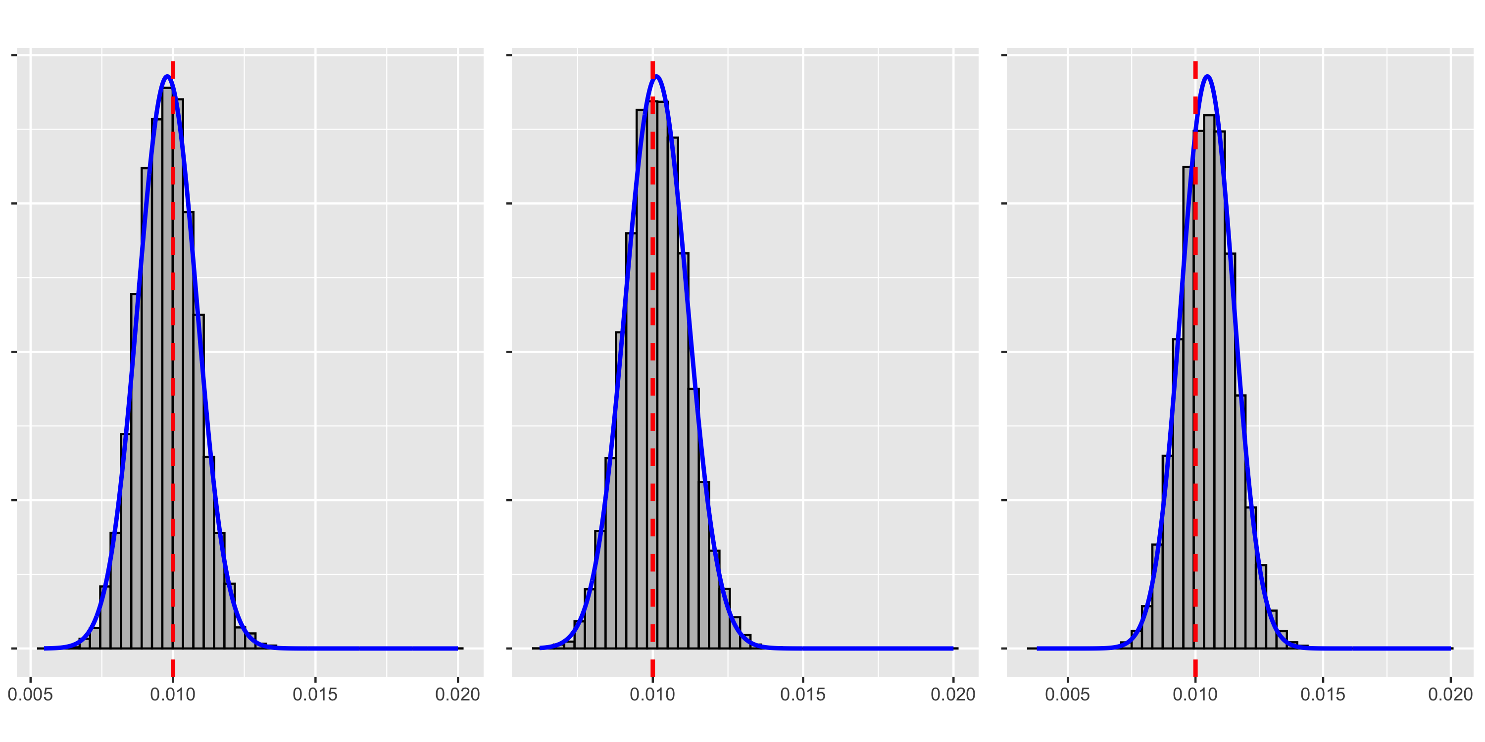
Figure 1: Approximations of the marginal posterior of $\theta$ obtained when running algorithm 1 on three different datasets with $\alpha=1$. The red line marks the true value of $\theta$ while the blue curve is the theoretical limiting distribution in Theorem 2.1. That is, a normal distribution centered at an efficient estimator (here the posterior mean) with variance the efficient Fisher information.

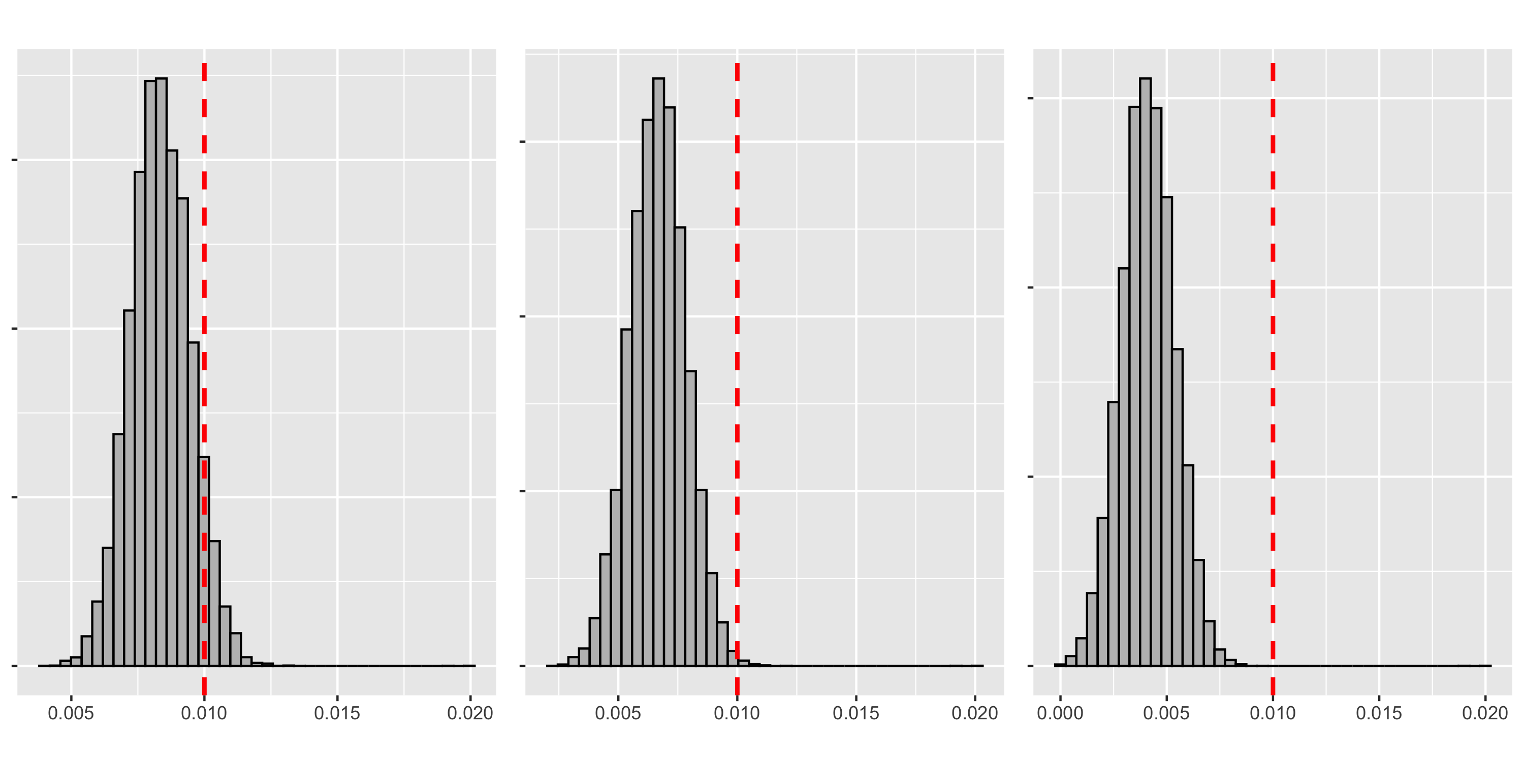
Figure 2: Approximations of the marginal posterior of $\theta$ for priors with regularity $\alpha$ equal to (from left to right) 2.6, 3.0 and 3.4. All three values of $\alpha$ are outside the BvM zone predicted by Theorem 2.1 The approximations are realized for the same dataset.

Overall, the presented figures validate the predictions of our semiparametric BvM. They also exhibit the positive relationship between the prior regularity $\alpha$ and the magnitude of a bias in the marginal posterior distributions which can be observed for $\alpha$ outside the BvM zone.

To verify the convergence of our sampling algorithm, we present two of the trace plots of the chains of $\theta$ obtained during the sampling process for different values of $\alpha$ and on different datasets. These trace plots showcase no particular behavior, and no burn in period seems to really be required to obtain convergence. This contributes to the evidence that our algorithm is indeed converging and sampling from the posterior distribution.

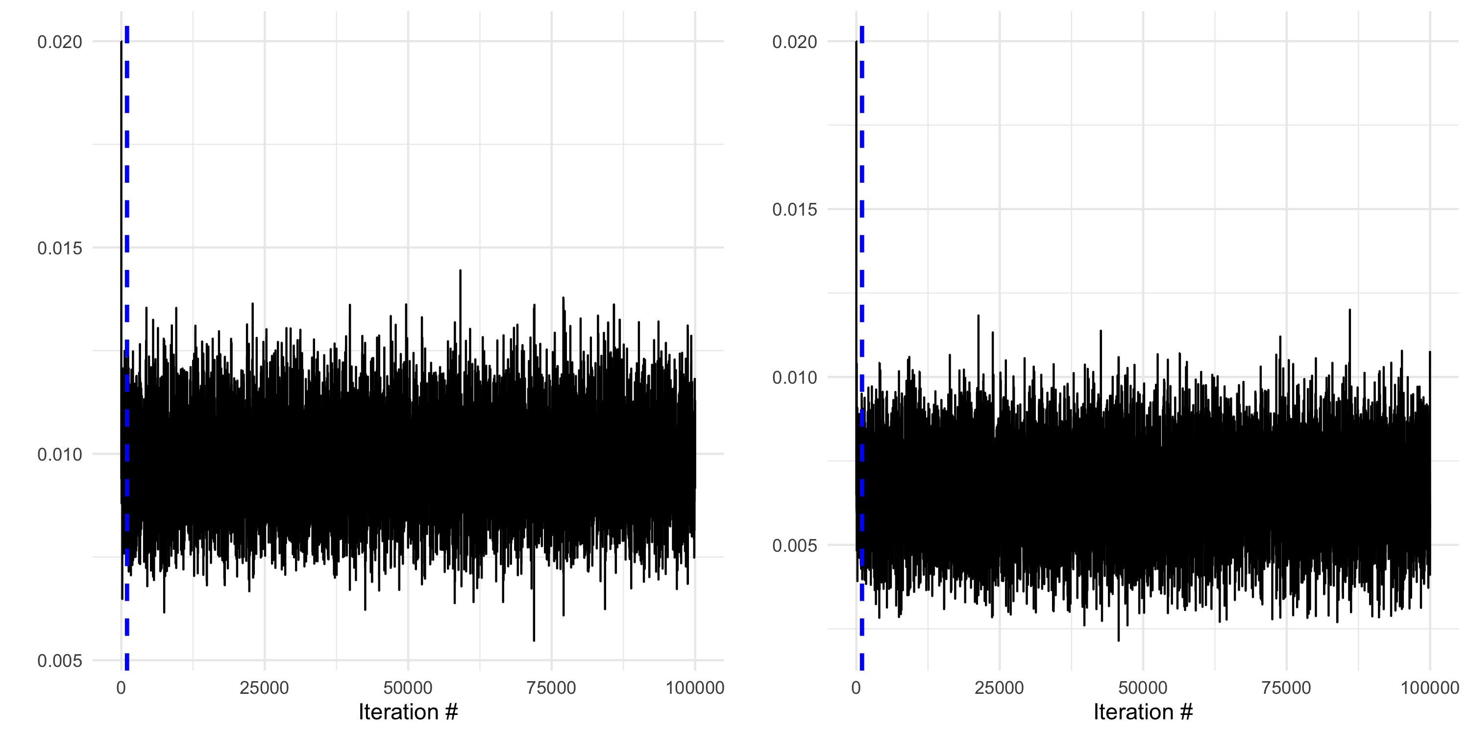
Figure 3: Trace plots of $\theta$ for two MH algorithm runs. The blue lines mark the burn in period selected.

5 Proof of Theorem 2.1

The proof relies on application of Theorem 2 of [2]. To set the stage we endow $L=\mathbb{R}\times L^{2}[0,1]$ with the inner product

$$\langle(a_{1},g_{1}),(a_{1},g_{2})\rangle_{L}=\langle g_{1},g_{2}\rangle+\langle K_{\theta_{0}}g_{1}+a_{1}\dot{K}_{\theta_{0}}f_{0},K_{\theta_{0}}g_{2}+a_{2}\dot{K}_{\theta_{0}}f_{0}\rangle,$$

with corresponding norm given by $\|a,g\|^{2}_{L}=\langle(a,g),(a,g)\rangle_{L}$. The LAN expansion (7) then reads

$$\log\frac{dP_{\theta_{0}+a/\sqrt{n},f+g/\sqrt{n}}}{dP_{\theta_{0},f_{0}}}=W(a,g)-\frac{1}{2}\|a,g\|^{2}_{L}+o_{P_{\theta_{0},f_{0}}}(1),$$

where

$$W(a,g)=\int g\,dW^{(1)}+\int(a\dot{K}_{\theta_{0}}f_{0}+K_{\theta_{0}}g)\,dW^{(2)},$$

with $W^{(1)}$ and $W^{(2)}$ independent $P_{\theta_{0},f_{0}}$-Brownian motions. Note that $W$ is the isonormal process on the Hilbert space $L$. Also observe that for the least favourable direction $\gamma=\gamma_{\theta_{0},f_{0}}$ it holds that $(0,\gamma)\in L$ is the orthogonal projection in $L$ of the point $(1,0)$ on the subspace $\{0\}\times L^{2}[0,1]$. Moreover, we have $\|1,0\|^{2}_{L}=\|\dot{K}_{\theta_{0}}f_{0}\|^{2}=I_{\theta_{0},f_{0}}$ and $\|0,\gamma\|^{2}_{L}=\langle K_{\theta_{0}}\dot{K}_{\theta_{0}}f_{0},(I+K^{2}_{\theta_{0}})^{-1}K_{\theta_{0}}\dot{K}_{\theta_{0}}f_{0}\rangle$, so that $\tilde{I}_{\theta_{0},f_{0}}=\|1,0\|^{2}_{L}-\|0,\gamma\|^{2}_{L}=\|1,-\gamma\|^{2}_{L}$. (Note that any $(a,g)\in L$ can be written as $(a,g)=a(1,-\gamma)+(0,g+a\gamma)$, where the terms are orthogonal in $L$. In particular, by Pythagoras, $\|a,g\|^{2}_{L}=a^{2}\tilde{I}_{\theta_{0},f_{0}}+\|0,g+a\gamma\|^{2}_{L}$.)

Let

$$R_{n}(\theta,f)=\log\frac{dP_{\theta,f}}{dP_{\theta_{0},f_{0}}}-\Big{(}\sqrt{n}W(\theta-\theta_{0},f-f_{0})-\frac{n}{2}\|\theta-\theta_{0},f-f_{0}\|^{2}_{L}\Big{)}$$

be the remainder in the LAN expansion. By Theorem 2 of [2] it suffices to show that there exist $\rho_{n}\to 0$, and $\gamma_{n}\in\mathbb{H}$ satisfying $\|\gamma_{n}-\gamma\|\to 0$ and $\|\gamma_{n}\|_{\mathbb{H}}^{2}\leq 2n\rho^{2}_{n}$, and $\varepsilon_{n}\to 0$ and $\mathcal{F}_{n}\subset L^{2}[0,1]$ such that with $\mathcal{F}_{n}(\theta)=\mathcal{F}_{n}+(\theta-\theta_{0})\gamma_{n}$, the following conditions are satisfied:

1. Posterior contraction: for some $c>0$ we have $\log\pi_{f}(\|f-f_{0}\|\leq c\varepsilon_{n})\lesssim n\varepsilon^{2}_{n}$ and

   $$\Pi((\theta,f)\in\Theta\times\mathcal{F}_{n}:\|\theta-\theta_{0},f-f_{0}\|_{L}\leq\varepsilon_{n}\,|\,X) \to 1,$$ (10)

   $$\inf_{|\theta-\theta_{0}|{\tilde{I}^{1/2}_{\theta_{0},f_{0}}}\leq\varepsilon_{n}}\Pi^{\theta=\theta_{0}}(f\in\mathcal{F}_{n}(\theta):\|0,f-f_{0}\|_{L}\leq\varepsilon_{n}/2\,|\,X) \to 1$$ (11)

   in $P_{\theta_{0},f_{0}}$-probability, where $\Pi^{\theta=\theta_{0}}$ is the posterior in the model in which $\theta=\theta_{0}$ is fixed.

2. Uniform LAN:

   $$\sup_{(\theta,f)\in\Theta\times\mathcal{F}_{n}\atop\|(\theta,f)-(\theta_{0},f_{0})\|_{L}\leq 2\varepsilon_{n}}\frac{R_{n}(\theta,f)-R_{n}(\theta_{0},f-(\theta-\theta_{0})\gamma_{n})}{1+n(\theta-\theta_{0})^{2}}\to 0$$

   in $P_{\theta_{0},f_{0}}$-probability.

3. Approximation of the least favourable direction: $\sqrt{n}\varepsilon_{n}\rho_{n}\to 0$.

The assumption $\varphi_{\gamma_{\theta_{0},f_{0}}}(\varepsilon_{n})\leq n\varepsilon^{2}_{n}$ implies that there exist $\gamma_{n}\in\mathbb{H}$ such that $\|\gamma_{n}-\gamma_{\theta_{0},f_{0}}\|\leq\varepsilon_{n}$ and $\|\gamma_{n}\|^{2}_{\mathbb{H}}\leq n\varepsilon^{2}_{n}$. We see that with this sequence $\gamma_{n}$ and $\rho_{n}=\|\gamma_{n}\|_{\mathbb{H}}/\sqrt{2n}$ we have $\rho_{n}\lesssim\varepsilon_{n}$ and $\sqrt{n}\varepsilon_{n}\rho_{n}\lesssim\sqrt{n}\varepsilon_{n}^{2}$, hence since $n\varepsilon^{4}_{n}\to 0$ condition (iii) above is satisfied. In the sections ahead we will prove that the posterior contraction and uniform LAN conditions (ii) and (iii) are satisfied for this sequence $\gamma_{n}$ as well.

The following lemma provides bounds for various norms and distances that we encounter in the proof. For $\eta\geq 0$ we denote the Sobolev-type space of regularity $\eta$ with respect to the sine basis by $S^{\eta}[0,1]$. This is the space of functions $f$ for which $\|f\|^{2}_{S^{\eta}}=\sum k^{2\eta}\langle f,e_{k}\rangle^{2}<\infty$. The operator norm of a bounded linear operator $T:L^{2}[0,1]\to S^{\eta}[0,1]$ is denoted by $\|T\|_{L^{2}\to S^{\eta}}=\sup_{\|f\|\leq 1}\|Tf\|_{S^{\eta}}$.

Lemma 5.1.

For all $f_{1},f_{2}\in\mathcal{F}$ and $\theta_{1},\theta_{2},\theta\in\Theta$ and $\eta\geq 0$ we have

1. $\|K_{\theta}\|\leq 1$, $\|\dot{K}_{\theta}\|\leq\frac{1}{2\theta}$,

2. $$\|{K_{\theta}-K_{\theta_{0}}}\|_{L^{2}\to S^{\eta}}\leq\frac{|\theta-\theta_{0}|}{\pi^{\eta}T^{\eta/2}}\Big{(}\frac{2+\eta}{2e(\theta_{0}\wedge\theta)}\Big{)}^{\frac{2+\eta}{2}},$$

3. $$\|K_{\theta}-K_{\theta_{0}}-(\theta-\theta_{0})\dot{K}_{\theta_{0}}\|_{L^{2}\to S^{\eta}}\leq\frac{(\theta-\theta_{0})^{2}}{2\pi^{\eta}T^{\eta/2}}\Big{(}\frac{4+\eta}{2e\theta_{0}}\Big{)}^{\frac{4+\eta}{2}},$$

4. $\|K_{\theta_{1}}f_{1}-K_{\theta_{2}}f_{2}\|\leq\|f_{1}-f_{2}\|+\frac{\pi}{2}\sqrt{\frac{T}{\theta_{1}\wedge\theta_{2}}}|\theta_{1}-\theta_{2}|(\|f_{1}\|\wedge\|f_{2}\|),$

5. $\|(K_{\theta}-K_{\theta_{0}})f_{0}\|\geq Te^{-(\theta\vee\theta_{0})\pi^{2}Tk^{2}}|\langle f_{0},e_{k}\rangle|\,|\theta-\theta_{0}|$ for all $k\geq 1$.

Proof.

(i). Follows from the explicit expressions for the operators and the inequality $\sup_{x\geq 0}x^{2}e^{-x}=4e^{-2}\leq 1$. (ii). We have

$$\|(K_{\theta} -K_{\theta_{0}})f\|^{2}_{S^{\eta}}$$

$$=\sum k^{2\eta}\langle f,e_{k}\rangle^{2}(e^{-\theta\pi^{2}Tk^{2}}-e^{-\theta_{0}\pi^{2}Tk^{2}})^{2}$$

$$\leq\sum k^{2\eta}\langle f,e_{k}\rangle^{2}e^{-2(\theta_{0}\wedge\theta)\pi^{2}Tk^{2}}((\theta-\theta_{0})\pi^{2}Tk^{2})^{2}$$

$$=\frac{(\theta-\theta_{0})^{2}}{2^{2+\eta}(\theta_{0}\wedge\theta)^{2+\eta}\pi^{2\eta}T^{\eta}}\sum\langle f,e_{k}\rangle^{2}e^{-2(\theta_{0}\wedge\theta)\pi^{2}Tk^{2}}(2(\theta_{0}\wedge\theta)\pi^{2}Tk^{2})^{2+\eta}.$$

Now use the fact that $\sup_{x\geq 0}e^{-x}x^{2+\eta}=e^{-(2+\eta)}(2+\eta)^{2+\eta}$. (iii). We have

$$\|(K_{\theta}-K_{\theta_{0}}-(\theta-\theta_{0})\dot{K}_{\theta_{0}})f\|^{2}_{S^{\eta}} =\sum k^{2\eta}\langle f,e_{k}\rangle^{2}e^{-2\theta_{0}\pi^{2}Tk^{2}}h^{2}((\theta-\theta_{0})\pi^{2}Tk^{2}),$$

where $h(x)=e^{-x}-1+x$. The proof is completed as the proof of (ii), using that $|h(x)|\leq x^{2}/2$ for $x\geq 0$ and $\sup_{x\geq 0}e^{-x}x^{4+\eta}=e^{-(4+\eta)}(4+\eta)^{4+\eta}$. (iv). By the triangle inequality and (i) we have $\|K_{\theta_{1}}f_{1}-K_{\theta_{2}}f_{2}\|\leq\|f_{1}-f_{2}\|+\|(K_{\theta_{1}}-K_{\theta_{2}})f_{2}\|$. By (3) and the inequalities $|e^{-x}-e^{-y}|\leq|x-y|e^{-x\wedge y}$ and $\sup_{x\geq 0}xe^{-x}=e^{-1}\leq 1/2$,

$$\|(K_{\theta_{1}}-K_{\theta_{2}})f_{2}\|^{2}\leq\frac{\pi^{2}T}{4(\theta_{1}\wedge\theta_{2})}(\theta_{1}-\theta_{2})^{2}\|f_{2}\|^{2}.$$

Since the same can be done with the roles of $f_{1}$ and $f_{2}$ reversed, we arrive at the desired inequality. (v). For every $k\geq 1$ we obviously have

$$\|(K_{\theta}-K_{\theta_{0}})f_{0}\|^{2} =\sum(e^{-\theta\pi^{2}Tj^{2}}-e^{-\theta_{0}\pi^{2}Tj^{2}})^{2}\langle f_{0},e_{j}\rangle^{2}$$

$$\geq(e^{-\theta\pi^{2}Tk^{2}}-e^{-\theta_{0}\pi^{2}Tk^{2}})^{2}\langle f_{0},e_{k}\rangle^{2}.$$

The inequality then follows from the elementary fact that $|e^{-x}-e^{-y}|\geq|x-y|e^{-x\vee y}$. ∎

5.1 Posterior contraction condition

In this section we consider conditions (10)–(11).

Items (i) and (v) of Lemma 5.1 and the triangle inequality imply that if $f_{0}\not=0$, there exists a constant $C>0$ such that

$$\|\theta-\theta_{0},f-f_{0}\|_{L}\leq Cd((\theta,f),(\theta_{0},f_{0})),$$

where the metric $d$ is defined by $d^{2}((\theta_{1},f_{1}),(\theta_{2},f_{2}))=\|f_{1}-f_{2}\|^{2}+\|K_{\theta_{1}}f_{1}-K_{\theta_{2}}f_{2}\|^{2}$. A straightforward adaptation of Theorem 8.31 of [10] then implies that (10) holds for a constant times $\varepsilon_{n}$ if for some $c_{0},c_{1},c_{2}>0$ we have

$$-\log\Pi((\theta,f):d((\theta,f),(\theta_{0},f_{0}))\leq c_{0}\varepsilon_{n}) \leq c_{1}n\varepsilon^{2}_{n}$$ (12)

$$\log N(\varepsilon_{n},\Theta\times\mathcal{F}_{n},d) \leq c_{2}n\varepsilon^{2}_{n},$$ (13)

$$\Pi((\theta,f)\not\in\Theta\times\mathcal{F}_{n}) \leq e^{-65c_{1}n\varepsilon^{2}_{n}}.$$ (14)

By part (iv) of Lemma 5.1 and the fact that $\Theta$ is bounded away from $0$ we have $d((\theta,f),(\theta_{0},f_{0}))\lesssim\|f-f_{0}\|+|\theta-\theta_{0}|$. Since the prior density for $\theta$ is bounded away from $0$, a sufficient condition for (12) is therefore that

$$-\log\pi_{f}(\|f-f_{0}\|\leq 2\varepsilon_{n})\lesssim n\varepsilon^{2}_{n}.$$

It is well known that this is equivalent to the concentration inequality $\varphi_{f_{0}}(\varepsilon_{n})\leq n\varepsilon^{2}_{n}$, see Lemma 5.3 of [21]. For the sieves $\mathcal{F}_{n}$ we take

$$\mathcal{F}_{n}=\varepsilon_{n}L^{2}_{1}+M\sqrt{n}\varepsilon_{n}\mathbb{H}_{1}$$

for appropriate $M>0$, where $\mathbb{H}_{1}$ and $L^{2}_{1}$ are the unit balls of the RKHS $\mathbb{H}$ and $L^{2}[0,1]$, respectively. Theorem 3.1 of [22] implies that (14) is fulfilled if $M$ is chosen large enough. It remains to check the entropy condition (13). Since $\mathbb{H}$ is continuously embedded in $L^{2}[0,1]$, we have that $\mathcal{F}_{n}\subset c^{\prime}M\sqrt{n}\varepsilon_{n}L^{2}_{1}$ for some $c^{\prime}>0$. Hence, by Lemma 5.1.(iv), we have

$$d((\theta_{1},f_{1}),(\theta_{2},f_{2}))\lesssim\|f_{1}-f_{2}\|+\sqrt{n}\varepsilon_{n}|\theta-\theta_{0}|$$

for all $\theta_{1},\theta_{2}\in\Theta$ and $f_{1},f_{2}\in\mathcal{F}_{n}$. It follows that

$$\log N(\varepsilon_{n},\Theta\times\mathcal{F}_{n},d)\lesssim\log N(\varepsilon_{n},\Theta,\sqrt{n}\varepsilon_{n}|\cdot|)+\log N(\varepsilon_{n},\mathcal{F}_{n},\|\cdot\|).$$

The first term is of order $\log n$ and the second one is bounded by a constant times $n\varepsilon^{2}_{n}$ by Theorem 3.1 of [22]. Hence, the assumption that $n\varepsilon^{2}_{n}\gtrsim\log n$ implies that the left-hand side of the display is bounded by a constant times $n\varepsilon^{2}_{n}$. We conclude that (12)–(14) are indeed fulfilled with $\mathcal{F}_{n}$ as above, so that condition (10) is satisfied.

The proof that (11) is satisfied is very similar, but now we need to bound the entropy of $\mathcal{F}_{n}(\theta)=\mathcal{F}_{n}+(\theta-\theta_{0})\gamma_{n}$ and the remaining mass $\pi_{f}(f\not\in\mathcal{F}_{n}(\theta))$, uniformly in $\theta$. For the entropy we note that if $\{f_{i}\}$ is an $\varepsilon$-net for $\mathcal{F}_{n}$ and $\{\theta_{j}\}$ is an $\delta$-net for $\Theta$, then $\{f_{i}+(\theta_{j}-\theta_{0})\gamma_{n}\}$ is an $(\varepsilon+\delta\|\gamma_{n}\|)$-net for $\mathcal{F}_{n}(\theta)$. Hence, by setting $\delta=\varepsilon/\|\gamma_{n}\|$ we get

$$\log N(2\varepsilon,\mathcal{F}_{n}(\theta),\|\cdot\|)\leq\log N(\varepsilon,\mathcal{F}_{n},\|\cdot\|)+\log\frac{\text{diam}(\Theta)\|\gamma_{n}\|}{\varepsilon}.$$

Since we have $\gamma_{n}\to\gamma$ and $n\varepsilon^{2}_{n}\gtrsim\log n$, it follows that $\log N(2\varepsilon_{n},\mathcal{F}_{n}(\theta),\|\cdot\|)\lesssim n\varepsilon^{2}_{n}$. Finally, for the remaining mass, we note that we can write $\mathcal{F}_{n}(\theta)=(\varepsilon_{n}L^{2}_{1}+(\theta-\theta_{0})\gamma_{n})+M\sqrt{n}\varepsilon_{n}\mathbb{H}_{1}$. Hence by the Borell-Sudakov-Tsirelson inequality,

$$\pi_{f}(f\not\in\mathcal{F}_{n}(\theta))\leq 1-\Phi(\Phi^{-1}(\pi_{f}(\|f-(\theta-\theta_{0})\gamma_{n}\|\leq\varepsilon_{n}))+M\sqrt{n}\varepsilon_{n}).$$

By Lemma 5.2 of [21],

$$\pi_{f}(\|f-(\theta-\theta_{0})\gamma_{n}\|\leq\varepsilon_{n})\geq e^{-\frac{1}{2}\|(\theta-\theta_{0})\gamma_{n}\|^{2}_{\mathbb{H}}}\pi_{f}(\|f\|\leq\varepsilon_{n})\geq e^{-K\text{diam}^{2}(\Theta)n\varepsilon^{2}_{n}}$$

for some $K>0$. Since $\Phi^{-1}(x)\sim-\sqrt{2\log(1/x)}$ for $x\to 0$, it follows that for given $C>0$, it holds that $\pi_{f}(f\not\in\mathcal{F}_{n}(\theta))\leq e^{-Cn\varepsilon^{2}_{n}}$, provided $M$ is chosen large enough. The proof that condition (11) holds is now easily completed.

5.2 Uniform LAN condition

Straightforward algebra gives

$$R_{n}(\theta,f) =\sqrt{n}\int(K_{\theta}-K_{\theta_{0}})(f-f_{0})\,dW^{(2)}$$

$$\quad+\sqrt{n}\int\Big{(}(K_{\theta}-K_{\theta_{0}})f_{0}-(\theta-\theta_{0})\dot{K}_{\theta_{0}}f_{0}\Big{)}\,dW^{(2)}$$

$$\quad-\frac{n}{2}\Big{\|}(K_{\theta}-K_{\theta_{0}})(f-f_{0})+\Big{(}(K_{\theta}-K_{\theta_{0}})f_{0}-(\theta-\theta_{0})\dot{K}_{\theta_{0}}f_{0}\Big{)}\Big{\|}^{2}$$

$$\quad-n\langle(K_{\theta}-K_{\theta_{0}})f_{0}-(\theta-\theta_{0})\dot{K}_{\theta_{0}}f_{0},K_{\theta_{0}}(f-f_{0})+(\theta-\theta_{0})\dot{K}_{\theta_{0}}f_{0}\rangle$$

$$\quad-n\langle(K_{\theta}-K_{\theta_{0}})(f-f_{0}),(\theta-\theta_{0})\dot{K}_{\theta_{0}}f_{0}\rangle$$

$$\quad-n\langle(K_{\theta}-K_{\theta_{0}})(f-f_{0}),K_{\theta_{0}}(f-f_{0})\rangle.$$

In particular we have $R(\theta_{0},f)=0$ for all $f$, so to verify the uniform LAN condition we need to show that $R_{n}(\theta,f)=o(1+n(\theta-\theta_{0})^{2})$, uniformly over the set $V_{n}=\{(\theta,f)\in\Theta\times\mathcal{F}_{n}:\|\theta-\theta_{0},f-f_{0}\|_{L}\leq 2\varepsilon_{n}\}$. Note that for $(\theta,f)\in V_{n}$ we have $\|f-f_{0}\|\lesssim\varepsilon_{n}$ and $|\theta-\theta_{0}|\lesssim\varepsilon_{n}$ and $\|f\|\lesssim 1+\varepsilon_{n}\lesssim 1$. We also repeatedly use the simple fact that $|x|\leq 1+x^{2}$, which implies that $\sqrt{n}/(1+n(\theta-\theta_{0})^{2})\leq 1/|\theta-\theta_{0}|$ and $\sqrt{n}|\theta-\theta_{0}|\leq 1+n(\theta-\theta_{0})^{2}$.

To deal with the first stochastic term, let

$$\mathcal{G}=\Big{\{}(\theta-\theta_{0})^{-1}(K_{\theta}-K_{\theta_{0}})(f-f_{0}):(\theta,f)\in V_{n}\Big{\}}.$$

We have $0\in\mathcal{G}$ and by Lemma 5.1.(ii) (applied with $\eta=0$) the $L^{2}$-diameter of $\mathcal{G}$ is bounded by a constant times $\varepsilon_{n}$. Part (ii) of Lemma 5.1 also shows that for every $\eta>0$, the set $\mathcal{G}$ belongs to a ball $B^{\eta}_{R\varepsilon_{n}}$ of radius $R\varepsilon_{n}$ in the Sobolev-type space $S^{\eta}[0,1]$ for some $R>0$. By Dudley’s theorem it follows that

$$\mathbb{E}\sup_{g\in\mathcal{G}}\Big{|}\int g\,dW^{(2)}\Big{|} \leq\mathbb{E}\sup_{g_{1},g_{2},\in\mathcal{G}\atop\|g_{1}-g_{2}\|\leq c\varepsilon_{n}}\Big{|}\int(g_{1}-g_{2})\,dW^{(2)}\Big{|}$$

$$\lesssim\int_{0}^{c\varepsilon_{n}}\sqrt{\log N(\varepsilon,B^{\eta}_{R\varepsilon_{n}},\|\cdot\|)}\,d\varepsilon$$

$$\lesssim\int_{0}^{c\varepsilon_{n}}\Big{(}\frac{\varepsilon_{n}R}{\varepsilon}\Big{)}^{1/(2\eta)}\,d\varepsilon=\varepsilon_{n}\int_{0}^{c}\Big{(}\frac{R}{x}\Big{)}^{1/(2\eta)}\,dx.$$

For $\eta>1/2$ the last integral is finite. Hence, we have

$$\sup_{\theta,f\in V_{n}}\frac{\sqrt{n}}{1+n(\theta-\theta_{0})^{2}}\Big{|}\int(K_{\theta}-K_{\theta_{0}})(f-f_{0})\,dW^{(2)}\Big{|}\leq\sup_{g\in\mathcal{G}}\Big{|}\int g\,dW^{(2)}\Big{|}\to 0$$

in probability.

For the second stochastic integral, consider

$$\mathcal{G}^{\prime}=\{(\theta-\theta_{0})^{-1}((K_{\theta}-K_{\theta_{0}})f_{0}-(\theta-\theta_{0})\dot{K}_{\theta_{0}}f_{0}):(\theta,f_{0})\in V_{n}\}.$$

By Lemma 5.1.(iii) (applied with $\eta=0$) we have $0\in\mathcal{G}^{\prime}$ and the $L^{2}$-diameter of $\mathcal{G}^{\prime}$ is bounded by a constant times $\varepsilon_{n}$. Part (iii) of Lemma 5.1 also implies that for every $\eta>0$, the set $\mathcal{G}$ belongs to a ball $B^{\eta}_{R\varepsilon_{n}}$ of radius $R\varepsilon_{n}$ in the Sobolev-type space $S^{\eta}[0,1]$ for some $R>0$. The uniform bound for the second stochastic integral is then obtained using Dudley’s theorem again.

It remains to consider the deterministic terms in the remainder. Using parts (ii) and (iii) of Lemma 5.1 (applied with $\eta=0$) and Cauchy-Schwarz it is straightforward to verify that the first three deterministic terms are $o(1+n(\theta-\theta_{0})^{2})$, uniformly over $V_{n}$. By Cauchy-Schwarz and part (ii) of Lemma 5.1 the last deterministic term is bounded by a constant times $n|\theta-\theta_{0}|\varepsilon_{n}^{2}=\sqrt{n}|\theta-\theta_{0}|\sqrt{n}\varepsilon_{n}^{2}$. This is $o(\sqrt{n}|\theta-\theta_{0}|)=o(1+n(\theta-\theta_{0})^{2})$ under the assumption that $\sqrt{n}\varepsilon^{2}_{n}\to 0$.

[Acknowledgments]

The authors would like to thank Frank van der Meulen and Aad van der Vaart for their helpful assistance and comments.

References

[1]{barticle}[author]
\bauthor\bsnmBissantz, \bfnmNicolai\binitsN. and \bauthor\bsnmHolzmann, \bfnmHajo\binitsH.
(\byear2008).
\btitleStatistical inference for inverse problems.
\bjournalInverse Problems
\bvolume24
\bpages034009, 17.
\bdoi10.1088/0266-5611/24/3/034009
\bmrnumber2421946
\endbibitem
[2]{barticle}[author]
\bauthor\bsnmCastillo, \bfnmIsmaël\binitsI.
(\byear2012).
\btitleA semiparametric Bernstein–von Mises theorem for Gaussian process
priors.
\bjournalProbability Theory and Related Fields
\bvolume152
\bpages53–99.
\endbibitem
[3]{barticle}[author]
\bauthor\bsnmCastillo, \bfnmIsmaël\binitsI. and \bauthor\bsnmRousseau, \bfnmJudith\binitsJ.
(\byear2015).
\btitleA Bernstein–von Mises theorem for smooth functionals in
semiparametric models.
\bjournalAnn. Statist.
\bvolume43
\bpages2353–2383.
\bdoi10.1214/15-AOS1336
\bmrnumber3405597
\endbibitem
[5]{bincollection}[author]
\bauthor\bsnmCavalier, \bfnmLaurent\binitsL.
(\byear2011).
\btitleInverse problems in statistics.
In \bbooktitleInverse problems and high-dimensional estimation.
\bseriesLect. Notes Stat. Proc.
\bvolume203
\bpages3–96.
\bpublisherSpringer, Heidelberg.
\bdoi10.1007/978-3-642-19989-9_1
\bmrnumber2868199
\endbibitem
[6]{barticle}[author]
\bauthor\bparticlede \bsnmJonge, \bfnmRené\binitsR. and \bauthor\bparticlevan \bsnmZanten, \bfnmHarry\binitsH.
(\byear2013).
\btitleSemiparametric Bernstein–von Mises for the error standard
deviation.
\bjournalElectron. J. Stat.
\bvolume7
\bpages217–243.
\bdoi10.1214/13-EJS768
\bmrnumber3020419
\endbibitem
[7]{bincollection}[author]
\bauthor\bsnmDunker, \bfnmT\binitsT.,
\bauthor\bsnmLifshits, \bfnmMA\binitsM. and \bauthor\bsnmLinde, \bfnmW\binitsW.
(\byear1998).
\btitleSmall deviation probabilities of sums of independent random variables.
In \bbooktitleHigh dimensional probability
\bpages59–74.
\bpublisherSpringer.
\endbibitem
[8]{barticle}[author]
\bauthor\bparticleet \bsnmal., \bfnmC. Chang\binitsC. C.
(\byear2019).
\btitleA unified analysis of four cosmic shear surveys.
\bjournalMonthly Notices of the Royal Astronomical Society
\bvolume482
\bpages3696-3717.
\endbibitem
[9]{barticle}[author]
\bauthor\bsnmGao, \bfnmP.\binitsP.,
\bauthor\bsnmHonkela, \bfnmA.\binitsA.,
\bauthor\bsnmRattray, \bfnmM.\binitsM. and \bauthor\bsnmLawrence, \bfnmN. D.\binitsN. D.
(\byear2008).
\btitleGaussian process modelling of latent chemical species: applications to
inferring transcription factor activities.
\bjournalBioinformatics
\bvolume24
\bpagesi70–i75.
\endbibitem
[10]{bbook}[author]
\bauthor\bsnmGhosal, \bfnmSubhashis\binitsS. and \bauthor\bparticleVan der \bsnmVaart, \bfnmAad\binitsA.
(\byear2017).
\btitleFundamentals of nonparametric Bayesian inference
\bvolume44.
\bpublisherCambridge University Press.
\endbibitem
[11]{barticle}[author]
\bauthor\bsnmGolubev, \bfnmG. K.\binitsG. K. and \bauthor\bsnmKhas’minskiĭ, \bfnmR. Z.\binitsR. Z.
(\byear1999).
\btitleA statistical approach to some inverse problems for partial
differential equations.
\bjournalProblemy Peredachi Informatsii
\bvolume35
\bpages51–66.
\bmrnumber1728907
\endbibitem
[12]{bbook}[author]
\bauthor\bsnmIbragimov, \bfnmIldar Abdulovich\binitsI. A. and \bauthor\bsnmHasminskii, \bfnmRafail Zalmanovich\binitsR. Z.
(\byear1981).
\btitleStatistical estimation: asymptotic theory.
\bpublisherSpringer.
\endbibitem
[13]{bbook}[author]
\bauthor\bsnmKaratzas, \bfnmIoannis\binitsI. and \bauthor\bsnmShreve, \bfnmSteven E.\binitsS. E.
(\byear1991).
\btitleBrownian motion and stochastic calculus,
\beditionsecond ed.
\bseriesGraduate Texts in Mathematics
\bvolume113.
\bpublisherSpringer-Verlag, New York.
\bdoi10.1007/978-1-4612-0949-2
\bmrnumber1121940
\endbibitem
[14]{barticle}[author]
\bauthor\bsnmKnapik, \bfnmB. T.\binitsB. T.,
\bauthor\bparticlevan der \bsnmVaart, \bfnmA. W.\binitsA. W. and \bauthor\bparticlevan \bsnmZanten, \bfnmJ. H.\binitsJ. H.
(\byear2013).
\btitleBayesian recovery of the initial condition for the heat equation.
\bjournalComm. Statist. Theory Methods
\bvolume42
\bpages1294–1313.
\bdoi10.1080/03610926.2012.681417
\bmrnumber3031282
\endbibitem
[15]{barticle}[author]
\bauthor\bsnmMair, \bfnmB. A.\binitsB. A.
(\byear1994).
\btitleTikhonov regularization for finitely and infinitely smoothing
operators.
\bjournalSIAM J. Math. Anal.
\bvolume25
\bpages135–147.
\bdoi10.1137/S0036141092238060
\bmrnumber1257145
\endbibitem
[16]{barticle}[author]
\bauthor\bsnmMair, \bfnmBernard A.\binitsB. A. and \bauthor\bsnmRuymgaart, \bfnmFrits H.\binitsF. H.
(\byear1996).
\btitleStatistical inverse estimation in Hilbert scales.
\bjournalSIAM J. Appl. Math.
\bvolume56
\bpages1424–1444.
\bdoi10.1137/S0036139994264476
\bmrnumber1409127
\endbibitem
[17]{bincollection}[author]
\bauthor\bsnmMcNeney, \bfnmBrad\binitsB. and \bauthor\bsnmWellner, \bfnmJon A.\binitsJ. A.
(\byear2000).
\btitleApplication of convolution theorems in semiparametric models with
non-i.i.d. data.
\bvolume91
\bpages441–480.
\bnotePrague Workshop on Perspectives in Modern Statistical Inference:
Parametrics, Semi-parametrics, Non-parametrics (1998).
\bdoi10.1016/S0378-3758(00)00193-2
\bmrnumber1814795
\endbibitem
[18]{barticle}[author]
\bauthor\bsnmStuart, \bfnmA. M.\binitsA. M.
(\byear2010).
\btitleInverse problems: a Bayesian perspective.
\bjournalActa Numer.
\bvolume19
\bpages451–559.
\bdoi10.1017/S0962492910000061
\bmrnumber2652785
\endbibitem
[19]{barticle}[author]
\bauthor\bparticlevan der \bsnmVaart, \bfnmAad\binitsA. and \bauthor\bparticlevan \bsnmZanten, \bfnmHarry\binitsH.
(\byear2007).
\btitleBayesian inference with rescaled Gaussian process priors.
\bjournalElectron. J. Stat.
\bvolume1
\bpages433–448.
\bdoi10.1214/07-EJS098
\bmrnumber2357712
\endbibitem
[20]{bbook}[author]
\bauthor\bparticlevan der \bsnmVaart, \bfnmA. W.\binitsA. W.
(\byear1998).
\btitleAsymptotic statistics.
\bseriesCambridge Series in Statistical and Probabilistic Mathematics
\bvolume3.
\bpublisherCambridge University Press, Cambridge.
\bdoi10.1017/CBO9780511802256
\bmrnumber1652247
\endbibitem
[21]{barticle}[author]
\bauthor\bparticlevan der \bsnmVaart, \bfnmA. W.\binitsA. W. and \bauthor\bparticlevan \bsnmZanten, \bfnmJ. H.\binitsJ. H.
(\byear2008).
\btitleReproducing kernel Hilbert spaces of Gaussian priors.
\bjournalPushing the Limits of Contemporary Statistics: Contributions in Honor
of Jayanta K. Ghosh
\bpages200–222.
\bdoi10.1214/074921708000000156
\endbibitem
[22]{barticle}[author]
\bauthor\bparticlevan der \bsnmVaart, \bfnmA. W.\binitsA. W. and \bauthor\bparticlevan \bsnmZanten, \bfnmJ. H.\binitsJ. H.
(\byear2008).
\btitleRates of contraction of posterior distributions based on Gaussian
process priors.
\endbibitem