Learning Probability Distributions of
Day-Ahead Electricity Prices

Abstract

We propose a novel machine learning approach to probabilistic forecasting of hourly day-ahead electricity prices. In contrast to recent advances in data-rich probabilistic forecasting that approximate the distributions with some features such as moments, our method is non-parametric and selects the best distribution from all possible empirical distributions learned from the data. The model we propose is a multiple output neural network with a monotonicity adjusting penalty. Such a distributional neural network can learn complex patterns in electricity prices from data-rich environments and it outperforms state-of-the-art benchmarks.

Keywords: Distributional forecasting, deep learning, probabilistic, electricity, energy time series

JEL: C45, C53, E17, E37

1  Introduction

“We will make electricity so cheap that only the rich will burn candles."

- Thomas A.Edison, 1880

Electricity is essential to modern life. Because its prices are inherently difficult to predict due to its complex, non-linear nature driven by the dynamics of supply and demand, incorporating uncertainty about future price movements is key to decision making in energy companies. While researchers have primarily focused on point forecasts over a long period of time, with weather-dependent renewable energy sources, turbulent times leading to increased imbalances between production and consumption, and higher price volatility (Maciejowska, 2020), research focusing on probabilistic price forecasting has recently gained importance (Nowotarski and Weron, 2018; Petropoulos et al., 2022). Probabilistic forecasting is rapidly becoming essential for producers, retailers and traders who need to assess uncertainty and improve optimal strategies for short-term operations, derivative pricing, value-at-risk, hedging and trading (Bunn et al., 2016).

Hand in hand with this surge in probabilistic electricity forecasting, researchers eager to use large numbers of series to understand fluctuations in electricity prices are collecting data unimaginable a few decades ago. With the explosion in the volume, velocity and variety of data, the need to unlock the information hidden in big data has become a key issue not only in energy economics (Diebold, 2021). Challenged by the proliferation of parameters and the strong criticism of arbitrarily chosen restrictions in both reduced and structured models in recent decades, economists wishing to explore the potentially rich information content of new datasets have recently turned their hopes to machine learning (Mullainathan and Spiess, 2017). A key idea of (machine) learning, which can be thought of as the inference of plausible models to explain observed data, has recently attracted a number of researchers who document how learning patterns from data can be useful (Mullainathan and Spiess, 2017; Sirignano et al., 2016; Gu et al., 2020; Heaton et al., 2017; Tobek and Hronec, 2020; Bianchi et al., 2020; Israel et al., 2020; Iworiso and Vrontos, 2020; Feng et al., 2018; Coulombe et al., 2020). A burgeoning literature and a growing number of applications in energy economics focus mostly on cross-sectional data and, ultimately, point forecasts. While machines can use such models to make predictions about future data, shifting the focus from point forecasting to probabilistic forecasting using big data is an essential next step.

The contribution of this paper is that we propose a novel machine learning approach to probabilistic forecasting of hourly day-ahead electricity prices. Our approach provides data-rich forecasts that are not constrained by distributional or other model assumptions, hence fully allows the exploration of non-Gaussian, heavy-tailed and asymmetric data. Our distributional neural network significantly outperforms state-of-the-art methods. Finally, we provide an efficient computational package.

Why should we believe that machine learning can improve probabilistic forecasting? Classical time series econometrics (Box et al., 2015; Hyndman et al., 2008) focuses mainly on predetermined autocorrelation or seasonality structures in data that are parameterised. With large amounts of time series available to researchers, these methods quickly become infeasible and unable to explore more complex data structures. Bearing in mind the famous adage that “all models are wrong…, but some of them are useful.” (Box et al., 1987), modern machine learning methods can easily overcome these problems. As a powerful tool for approximating complex and unknown data structures (Kuan and White, 1994), these methods can be useful in a range of application problems where data contain a rich information structure that cannot be satisfactorily described by a simplifying model. Overcoming the long-standing problem of computational intensity of such data-driven approach with advances in computer science adds to the temptation to use these methods to address new problems such as distribution prediction.

The use of machine learning methods is also emerging in the literature on hourly electricity price forecasting. Lago et al. (2021); Lehna et al. (2022); Zhang et al. (2022) use a hybrid recurrent network for point forecasts. Nowotarski and Weron (2018) reviews recent advances in probabilistic forecasting, while Mashlakov et al. (2021) uses probabilistic forecasting with auto-regressive recurrent networks (DeepAR) developed by Amazon Research Germany (Salinas et al., 2020). Marcjasz et al. (2020) also uses non-linear autoregressive networks with exogenous variables, Klein et al. (2023) constructs deep recurrent networks. Mashlakov et al. (2021) assesses the performance of deep learning models for multivariate probabilistic forecasting, and Marcjasz et al. (2023) uses a deep neural network with output from the normal and Johnson’s SU distributions.

All these approaches rely on restrictive models and assumptions, particularly, the literature usually proposes to learn only some features of the distribution, such as moments. In contrast, our approach selects the best distribution from all possible empirical distributions learned from the data.

In this paper, we propose a deep learning method that overcomes these problems and provides information-rich uncertainty forecasts of electricity prices. Specifically, we propose a distributional neural network to provide probabilistic forecasts that reflect the time-series dynamics of large amounts of available information relevant to future prices. Such data-driven probabilistic forecasts aim to improve the current state of the art in forecasting and communicating uncertainty.

In the empirical exercise, we build a distributional network to forecast German hourly day-ahead electricity prices using the 221 characteristics, including lagged prices, total load, external variables such as EU allowance prices, fuel prices, in particular coal, gas and oil. Such data-rich uncertainty forecasts, which do not rely on distributional assumptions or model choice, are the first of their kind. To benchmark our framework, we use the naive model and the two quantile regression-based linear models with autoregressive and exogenous variables: quantile regression averaging and quantile regression committee machine Nowotarski and Weron (2015); Marcjasz et al. (2020) estimated with lasso estimated autoregression. Our model significantly outperforms the benchmarks.

2  Probabilistic forecasting via distributional neural network

Consider hourly day-ahead electricity time series $y_{t,h}$ collected over $t=1\ldots,T$ days and $h=1,\ldots,24$ hours. The main objective is to approximate as closely as possible the conditional cumulative distribution function $F(y_{t,h}|\mathcal{I}_{t-1})$ and use it for a $1$-step-ahead probabilistic forecast made at time $t-1$ with information $\mathcal{I}_{t-1}$ containing past values of $y_{t,h}$ and possibly past values of other exogenous observable variables $x_{t}$.

The main goal is then to approximate a collection of conditional probabilities corresponding to the empirical quantiles, such as

$$\Big{\{}F(q_{h}^{\alpha_{1}}),\ldots,F(q_{h}^{\alpha_{p}})\Big{\}}=\Big{\{}\Pr\Big{(}y_{t,h}\leq q_{h}^{\alpha_{1}}|\mathcal{I}_{t-1}\Big{)},\ldots,\Pr\Big{(}y_{t,h}\leq q_{h}^{\alpha_{p}}|\mathcal{I}_{t-1}\Big{)}\Big{\}}$$

for the collection of thresholds $1,\ldots,p$. A convenient way to estimate such quantities is distribution regression. Foresi and Peracchi (1995) noted that several binary regressions serve as good partial descriptions of the conditional distribution. To estimate the conditional distribution, one can simply consider a distributional regression model with a (monotonically increasing) link function, such as logit, probit, linear, log-log functions. In contrast to estimating separate models for separate thresholds, Chernozhukov et al. (2013) considered a continuum of binary regressions and argued that it provides a coherent and flexible model for the entire conditional distribution as well as a useful alternative to Koenker and Bassett Jr (1978)’s quantile regression. Alternatively, Anatolyev and Baruník (2019) suggest binding the coefficients of predictors in an ordered logit model via smooth dependence on corresponding probability levels. While this approach is able to predict the entire distribution, keeping $0<F_{j}<1$ and $0<F_{1}(.)<F_{2}(.)<\dots F_{p}(.)<1$, it still depends on a strong parameterisation suited to a specific problem of the time series considered, making it an unfeasible approach for a larger number of variables.

2.1  Distributional neural network

Such probabilistic predictions are highly dependent on the model parameterisation and quickly become infeasible with increasing number of covariates. This motivates us to reformulate distributional regression into a more general and flexible distributional neural network. The functional form of the new network is driven by the data, and we can relax assumptions about the distribution of the data, the parametric model as well as the stationarity of the data. The proposed distributional neural network, as a feed-forward network, is a hierarchical chain of layers representing high-dimensional and/or non-linear input variables with the aim of predicting the target output variable. Importantly, we approximate the conditional distribution function with multiple outputs of the network as a set of joint probabilities.

As a first step, we replace a known link function with an unknown general function $\mathfrak{g}$, which is approximated by a neural network. Next, we consider a set of probabilities corresponding to $0<\alpha_{1}<\alpha_{2}<\ldots<\alpha_{p}<1$ being $p$ regularly spaced levels that characterise the conditional distribution function using a set of predictors $\boldsymbol{z}_{t}$ to be specified later, and model them jointly as

$$\Big{\{}\Pr\Big{(}y_{t,h}\leq q_{h}^{\alpha_{1}}|\boldsymbol{z}_{t-1}\Big{)},\ldots,\Pr\Big{(}y_{t,h}\leq q_{h}^{\alpha_{p}}|\boldsymbol{z}_{t-1}\Big{)}\Big{\}}=\mathfrak{g}_{W,b,h}(\boldsymbol{z}_{t-1}),$$ (1)

where $\mathfrak{g}_{W,b,h}$ is a multiple output neural network with $L$ hidden layers that we name as distributional neural network:

$$\mathfrak{g}_{W,b,h}(\boldsymbol{z}_{t-1})=g^{(L)}_{W^{(L)},b^{(L)}}\circ\ldots\circ g^{(1)}_{W^{(1)},b^{(1)}}\left(\boldsymbol{z}_{t-1}\right),$$ (2)

where $W=\left(W^{(1)},\ldots,W^{(L)}\right)$ and $b=\left(b^{(1)},\ldots,b^{(L)}\right)$ are weight matrices and bias vector. Any weight matrix $W^{(\ell)}\in\mathbb{R}^{m\times n}$ contain $m$ neurons as $n$ column vectors $W^{(\ell)}=[w_{\cdot,1}^{(\ell)},\ldots,w_{\cdot,n}^{(\ell)}]$, and $b^{(\ell)}$ are thresholds or activation levels.

It is important to note that, in contrast to the literature, we consider a multi-output (deep) neural network to characterise the collection of probabilities. Before discussing the estimation details that allow us to preserve the monotonicity of the probabilities, we illustrate the framework. Figure  1 illustrates how $l\in{1,...,L}$ hidden layers transform input data into a chain using a collection of non-linear activation functions $g^{(1)},\ldots,g^{(L)}$. A commonly used activation function, $g^{(\ell)}_{W^{(\ell)},b^{(\ell)}}$, is used as the

$$g^{(\ell)}_{W^{(\ell)},b^{(\ell)}}:=g_{\ell}\left(W^{(\ell)}\boldsymbol{z}_{t-1}+b^{(\ell)}\right)=g_{\ell}\left(\sum_{i=1}^{m}W^{(\ell)}_{i}\boldsymbol{z}_{t-1}+b_{i}^{(\ell)}\right)$$

are a sigmoid $g_{\ell}(u)=\sigma(u)=1/(1+\exp(-u))$, rectified linear units $g_{\ell}(u)=\max\{u,0\}$, or $g_{\ell}(u)=\tanh(u)$. In case $\mathfrak{g}_{W,b,h}(u)$ is non-linear, neural network complexity grows with increasing number of neurons $m$, and with increasing number of hidden layers $L$ and we build a deep neural network. We use activation function $g^{(L)}(\cdot)=\sigma(\cdot)$ to transform outputs to probabilities. Note that for $L=1$, neural network becomes a simple logistic regression.

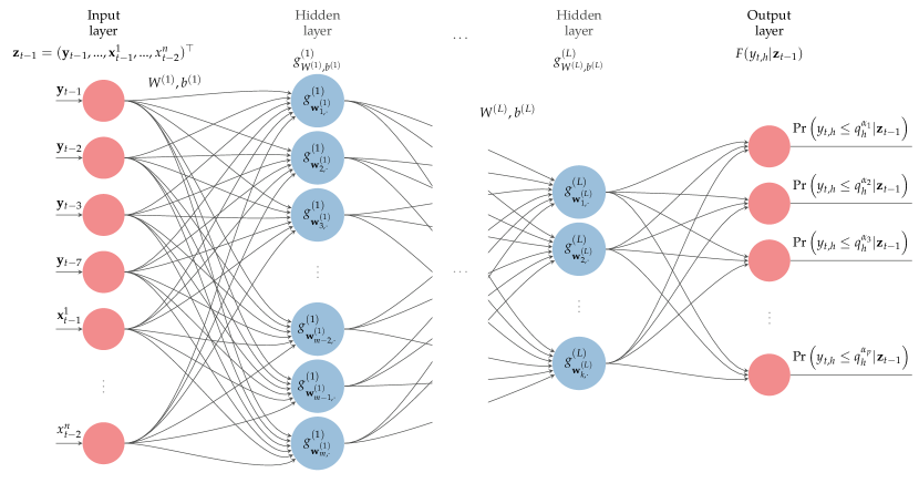
Figure 1: Distributional (Deep) Feed-forward Network.

An illustration of a multiple output (deep) neural network $\mathfrak{g}_{W,b,h}(\boldsymbol{z}_{t-1})$ to model the collection of conditional probabilities $\Big{\{}\Pr\Big{(}y_{t,h}\leq q_{h}^{\alpha_{1}}|\boldsymbol{z}_{t-1}\Big{)},\ldots,\Pr\Big{(}y_{t,h}\leq q_{h}^{\alpha_{p}}|\boldsymbol{z}_{t-1}\Big{)}\Big{\}}$ with set of predictor variables $\boldsymbol{z}_{t}=(\boldsymbol{y}_{t},\boldsymbol{x}_{t}^{1},...,\boldsymbol{x}_{t}^{n})^{\top}$. With large number of hidden layers $L$ the network is deep.

2.2  Loss Function

Since we want to estimate the cumulative distribution function (CDF), which is a non-decreasing function bounded on $[0,1]$, we need to design an objective function that minimises the differences between the target and the estimated distribution, as well as imposing a non-decreasing property on the output. As the problem is essentially a more complex classification problem, logistic regression, we use a binary cross-entropy loss function. In addition, we introduce a penalty to the multiple output classification problem to order the predicted probabilities.

The loss function is then composed of two parts: traditional binary cross-entropy and a penalty adjusting for monotonicity of predicted output:

$$\mathcal{L} = -\frac{1}{T}\sum_{t}^{T}\underbrace{\frac{1}{p}\sum_{j}^{p}\left(\mathbb{I}\{y_{t,h}\leq q_{h}^{\alpha_{j}}\}\log\left\{\widehat{\mathfrak{g}}_{W,b,h,j}(\boldsymbol{z}_{t-1})\right\}+\left(1-\mathbb{I}\{y_{t,h}\leq q_{h}^{\alpha_{j}}\}\right)\log\left\{1-\widehat{\mathfrak{g}}_{W,b,h,j}(\boldsymbol{z}_{t-1})\right\}\right)}_{\text{\text{binary cross-entropy}}}$$ (3)

$$+\leavevmode\nobreak\ \underbrace{\lambda_{m}\sum_{t}^{T}\sum_{j=1}^{p-1}\left(\widehat{\mathfrak{g}}_{W,b,h,j}(\boldsymbol{z}_{t-1})-\widehat{\mathfrak{g}}_{W,b,h,j+1}(\boldsymbol{z}_{t-1})\right)_{+}}_{\text{\text{monotonicity penalty}}}$$

where $(u)_{+}$ is a rectified linear units function, ReLU, $(u)_{+}=\max\{u,0\}$, which passes through only positive differences between two neighbouring values, $j$ and $j+1$, of CDF, those violating the monotonicity condition, and $\mathbb{I}\{.\}$ is an indicator function. This violation is controlled by the penalty parameter $\lambda_{m}$. Note that in addition to its simplicity, ReLU is used for convenience reasons allowing for general use.

3  Data

We use the spot market price, which is important for day-ahead auctions. In the day-ahead electricity market, the day-ahead forecast is used to formulate bids for 24 hours, which generally means that on day $t-1$ participants submit bids for the 24 hours of the day-ahead. These are executed up to a certain hour (deadline), after which the market clears and participants receive energy allocations at the clearing price. We consider the hourly day-ahead electricity market in Germany. The data cover the period from 7 January 2015 to 31 December 2020.

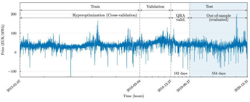
Figure 2: Electricity price data with distinguished and depicted periods for estimation. Train and Validation subsamples show how much of data is used for training the model at both stages, hyper-optimization training and rolling window learning.

To carry out the forecasting exercise of day-ahead electricity prices $y_{t,h}$ with hourly observations, we partition the data, in machine learning jargon, into train, validation, and test sets. As illustrated in Figure 2, we consider the last 736 days, period as the test subsample (out-of-sample, OOS). The days prior to OOS are used as training and estimation, which we split into train and validation parts. The block QRA validation is the first 182 days of OOS partition are used as a calibration window for the quantile regression as calibration window, thus we do not consider this part when we evaluate OOS results of the distributional neural network. This leaves us with last 554 days period between 2019-06-07 and 2020-12-31, which is a sufficient number of days considered for good practice to evaluate techniques in the EPF literature. Test subsample (out-of-sample, OOS) is never available to the learning algorithm while training the model. We further divide the train subsample into training and validation sets, which are used to cross-validation of neural network and to find its parameters selection.

3.1  Data transformation

Prior to the estimation procedure, we transform the data, as is common in the EPF literature, in order to stabilise its variance and make the distribution more symmetrical. Since German electricity prices are allowed to be negative, we cannot use a logarithmic transformation. We adopt the variance-stabilising transformation of Uniejewski et al. (2018) in its simpler form, as also discussed in Narajewski and Ziel (2020). We do the median normalisation of the price, $p_{t,h}$, as $p^{n}_{t,h}=1/b(p_{t,h}-\widehat{a})$, where $\widehat{b}=\text{MAD}(p_{t,h|\mathcal{I}_{t-1}})1/z_{0.75}$, $\widehat{a}=\text{median}(p_{t,h|\mathcal{I}_{t-1}})$, and $1/z_{0.75}=1.4826$ is the 75% quantile of $\mathcal{N}(0,1)$. After this first step, we apply inverse hyperbolic transformation such that $y^{n}_{t,h}=\text{asinh}(p^{n}_{t,h})$ to obtain more variance stable and symmetric price data.

To get the data back to the original scale, we do the transformation in the inverse order such that $\widehat{\mathbb{E}(p_{t,h})}=\widehat{\mathbb{E}(y_{t,h})}\cdot\widehat{b}+\widehat{a}\approx\sinh(\widehat{\mathbb{E}(y_{t,h})})\cdot\widehat{b}+\widehat{a}$, where $\widehat{\mathbb{E}(y_{t,h})})$ is a model forecast for the price (quantiles), sinh is the hyperbolic sin function, and $\widehat{b}$ and $\widehat{a}$ are sample parameters of the transformation, MAD and median, respectively. In Figure 3, we plot histograms of day-ahead price prior and after the transformation showing changes in scale and shape.

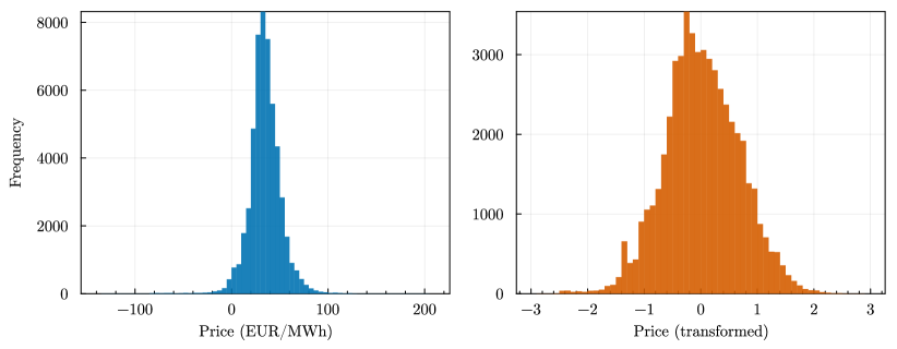
Figure 3: Histogram of original and transformed price data.

3.2  Input variables

Based on the data provided by Marcjasz et al. (2023), a consistent approach is taken for constructing the inputs for all models. The input features correspond to the day-ahead price data at their respective time points, resulting in 24 hour-ahead prices denoted by $\boldsymbol{y}_{t}=[y_{t,1},\dots y_{t,24}]$. The inputs $\boldsymbol{z}_{t-1}$ constitute the information set $\mathcal{I}_{t-1}$, which includes historical price data and other exogenous variables.

However, as neural networks estimate time-dependent variables with intricate and non-linear relationships, it remains necessary to provide time-series lagged inputs, since the data are autocorrelated and seasonal patterns such as daily and weekly are present. Therefore, we begin by incorporating previous day-ahead prices as lags, specifically $\boldsymbol{y}_{t-1}$, $\boldsymbol{y}_{t-2}$, $\boldsymbol{y}_{t-2}$, and $\boldsymbol{y}_{t-7}$. Next, the variable total load is significant in the EPF studies as it’s a targeted variable. We incorporate all hours of the day-ahead forecast for the previous two days, including $\boldsymbol{x}^{1}_{t}$, $\boldsymbol{x}^{1}_{t-1}$, and $\boldsymbol{x}^{1}_{t-7}$. The final variable to be incorporated in the 24-hour size pertains to a day-ahead prediction of renewable energy sources. For this, we include data for the day ahead and the prior day, $\boldsymbol{x}^{2}_{t}$ and $\boldsymbol{x}^{2}_{t-1}$. Other external variables to be included are the closing prices of EU allowances, ${x}^{3}_{t-2}$, and the prices of fuels, in particular coal, gas and oil, ${x}^{4}_{t-2}$, ${x}^{5}_{t-2}$ and ${x}^{6}_{t-2}$. Since we forecast $(t)$ today, these costs reflect the most recent data available, from two days ago, following the standard practice of the day-ahead auction market. Finally, to address the weekly pattern in the data, we incorporate a vector of weekday dummies, ${x}^{7}_{t,weekday}$ for the specific day of the week. Total number of columns in the input matrix is 221 features. We consider inputs $\boldsymbol{z}_{t}=[\boldsymbol{y}_{t-1},\boldsymbol{y}_{t-2},\boldsymbol{y}_{t-3},\boldsymbol{y}_{t-7},\boldsymbol{x}^{1}_{t},\boldsymbol{x}^{1}_{t-1},\boldsymbol{x}^{1}_{t-7},\boldsymbol{x}^{2}_{t},\boldsymbol{x}^{2}_{t-1},{x}^{3}_{t-2},{x}^{4}_{t-2},{x}^{5}_{t-2},{x}^{6}_{t-2},{x}^{7}_{t,weekday}]$ for all models except the naive one.

3.3  Target variable and the information set

To forecast the probability of the day-ahead electricity price being below specific quantile levels, we model it as a set of probabilities based on the conditional price information set, i.e. $\Pr\left(y_{t,h}\leq q_{h}^{\alpha_{j}}|\mathcal{I}_{t-1}\right)$. When forecasting, it is crucial to ensure the information set is set accurately. The previous observations prior to the day on which the forecast is made make up the information set $\mathcal{I}_{t-1}$. In our setup, we consider the data of the training and validation subsamples available to the information set.

The accuracy of the forecast outcomes is largely dependent on the precisely defined empirical quantiles, $q_{h}^{\alpha}$, which correspond to a set of probabilities $\{\alpha\}$. Due to different location, size, and shape that influence hourly price distributions, target variable is on an hourly basis. The predicted variable is a set of hourly indicators related to $p$ equidistant probability levels $\alpha_{j}=\{0.01,\dots,0.99\}$, where $p=31$. As a result, the target variable is

$$\boldsymbol{y}_{t,h,\alpha_{j}}=\mathbb{I}\{y_{t,h}\leq q_{h}^{\alpha_{j}}|\mathcal{I}_{t-1}\},\text{ for }h=1,...,24,\forall\alpha_{j}.$$ (4)

The unconditional quantiles defined by hours allow us to assume that the distribution within the information set is hour specific.

Last, the data for the target variable are subjected to winsorisation, we use a proportion of 0.1% to deal with the extreme minimum and maximum values within the information set. Eq. 4 shows that the cumulative distribution function approximation approach uses unconditional quantiles $q^{\alpha_{j}}$ for the indicator of the target variable. Winsorisation with a small fraction has no effect because the lowest and highest $\alpha$ values are less than 0.1%. The handling of extreme outliers, e.g. negative prices, is beneficial in the post-estimation inverse transformation of $\widehat{F}(y_{t,h})$ into $\widehat{F}^{-1}(\alpha)$, where we follow Fritsch and Carlson (1980).

4  Estimation

We begin by presenting the forecasting setup and outlining our approach of non-parametric distributional neural network procedure. Next, we propose benchmark models, such as the naive model, and then consider two versions of quantile regression based on a linear model with autoregressive and exogenous variables (Nowotarski and Weron, 2018; Serafin et al., 2019; Marcjasz et al., 2023), which are stable benchmarks in the probabilistic electricity price forecasting literature. The bids in the auctions are posted once a day for all hours, we follow the literature (Maciejowska et al., 2016; Liu et al., 2017) and predict the distributions of day-ahead prices for each hour given the same information for all hours.

4.1  Distributional neural network

In line with the saying, “a picture is worth a thousand words”, we present cumulative distribution functions and quantile functions in Figure 4, which encapsulate the idea of how we obtain distributional forecast, from left to right. The left panel illustrates the approximation of CDFs for every day and hour using $p$ equidistant points that correspond to $\alpha_{j}$ probabilities. In the plot on the right, we show the predicted 99 quantiles of day-ahead prices for given hours, obtained by inversion and interpolation. Both figures are based on the unconditional values of the complete data set. Nonetheless, they demonstrate how our results look for a single forecasted day of 24 hours.

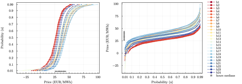
Figure 4: Unconditional cumulative distribution, $F_{h}(y_{y,h})$, and quantile functions by hours (depicted by warm to cold colors), $Q_{h}(\alpha)$, for whole data sample. Left: Illustrates 31 $\alpha$ probability levels used to provide our target variable and similar to these unconditional CDF we train the conditional one. Right: Unconditional quantiles for 99 $\alpha$ probability levels mimic the final result of distributional forecasts.

Our distributional neural network is a multilayer perceptron, it has two (possibly more) hidden layers, with each layer containing different numbers of neurons, which are fine-tuned by hyper-optimization. The DistrNN’s input size is 221 features, which is taken in. We make no assumptions regarding the shape of distributions, as DistrNN directly outputs the vector of probabilities, which are 31 values approximating the CDF. We allow for a different distribution for each hour and as a result, we have twenty-four distributional neural networks to train.

To develop and analyse the model, we utilise the Julia programming language, specifically using the Flux.jl package (Innes et al., 2018) for neural network training. Most neural networks have essential components, such as optimisation algorithms and techniques to prevent over-fitting. We implement AdamW (Loshchilov and Hutter, 2019) as our optimisation algorithm, which includes regularisation techniques. AdamW mimics $L_{2}-norm$ regularisation through its weight decay as learning occurs. Then, we apply dropout regularization method (Srivastava et al., 2014) and batch normalization to the first layer’s weights in the model. The learning rate for stochastic gradient descent (Adam, Kingma and Ba (2014)), denoted as $\eta$, the weight decay regularising parameter, denoted as $\lambda_{W}$, and the proportion parameter for dropout, indicating how many neurons to turn off in each layer, denoted as $\phi$, are subjected to hyper-optimisation.

4.1.1  Training and hyper-optimization tuning

Our forecasting procedure is similar to other forecasting studies that make use of a daily data forward rolling scheme. We use data from a training and validation period consisting of four and a half years (shown in Figure 2) to perform a hyper-optimization search for parameters. To reduce computational costs, the hyper-optimization is conducted before implementing the rolling window scheme. We use k-folds cross validation on randomly shuffled data to increase the possibility of model generalisation rather than data memorisation. The dataset is divided into seven cross-validation sets, with data being separated into a 1:7 train-validation ratio. We must determine the ideal parameters for the distributional neural network for every hour of the day-ahead prices. For hyper-optimization, the algorithm considers 60 parameter combinations in a grid fashion based on the parameter ranges and sets provided in Table 1. The top parameters set is that with the smallest mean of validation losses from cross-validation. We run our neural network for a maximum of 1000 epochs. Additionally, we employ early stopping with a patience of 15 epochs when the validation loss does not show improvement. Furthermore, we utilise batches of 64 data points. The input data for DistrNN are augmented with with noise from $\mathcal{N}(0,0.1)$.

Hyper parameters	Values		Fixed parameters	Value
Learning rate, $\eta$	$Range_{1}(0.0001,0.003)$		Number of HPO combinations	60
Dropout rate, $\phi$	$Range_{2}(0.0,1.0)$		Epochs	1000
$L_{2}$-decay rate, $\lambda_{W}$	$Range_{2}(0.000001,0.01)$		Early stopping patience	15
Hidden neurons in each layer	$Range_{2}(32,384)$		Monotonicity, $\lambda_{m}$	1.5
Mini batch size	$\{64\}$		Number of layers	2
Activation functions	$\{$relu, tanh, sigmoid, softmax$\}$		$\alpha$ levels	31
			CV k-folds	7
			Ensembles	8

Table 1: Parameter values used to train distributional neural network.

The hyper-optimization algorithm searches through the space of hyperparameters and randomly tries a number of parameters sets to train a network. $Range_{1}$ is evenly spaced log range, $Range_{2}$ is evenly spaced linear range.

4.1.2  Forward rolling forecasting (recalibration)

We evaluate the models on the out-of-sample period of 736 days, shown as a test in Figure 2, with focus on the shaded area of the last 554 days. Starting from 12 December 2018, we train DistrNN using a tuned parameter set for each hour of the day in a rolling window fashion. To train DistrNN, we minimise the loss given by the binary cross entropy function (Eq. 3). In this part, we keep four and a half years of data available for training, and the split is with a ratio of 80% for training and 20% for validation subsamples of shuffled data. To reduce the forecast variance, we train the model several times with different initialisation of weights and biases. Taking into account the validation loss, we only consider the first better half of the results, i.e. with an ensemble size of $n=8$ forecasts, we consider the first four, $\{\widehat{F}_{1},\widehat{F}_{2},\dots,\widehat{F}_{n/2}\}$.

The distributional neural network predicts a CDF, $\widehat{F}_{t,h}(\cdot|\mathcal{I}_{t-1})$, which we use to find its inverse, $\widehat{F}^{-1}(y_{t,h})=\widehat{Q}(\alpha)$, which is the quantile function, more precisely a collection of quantiles for a given $\alpha_{j}=\{0.01,\dots,0.99\}$. Before the inversion, we use the monotone cubic interpolation of (Fritsch and Carlson, 1980). On the interval [0,1] we obtain a monotonically increasing CDF on a finite grid of 400 points. We find the inverse function before aggregating the predicted DistrNN CDFs $\widehat{F}^{i}_{t,h}$. Thus, in the case of neural networks, the aggregated ensemble mean is the mean of the predictions. We average the predictions over the quantiles $\bar{Q}(\alpha)=\frac{1}{N_{ens}}\sum_{i}^{N_{ens}}\widehat{F}^{-1}_{i}(y)$, and evaluate $\bar{Q}_{t,h}(\alpha)$ as our result. Note that we consider ensembles over quantiles rather than probabilities, although both quantile and probability averaging of out-of-sample ensembles give similar results in Marcjasz et al. (2023).

We face the inverse problem of quantile crossing: possible violation of monotonicity of the cumulative distribution function. To solve this, we propose a loss function (Eq. 3) that penalises for such occurrences. During learning, the algorithm only retains models with parameters that satisfy the monotonicity condition during learning.

4.2  Naive benchmark

To be consistent with the literature, we use the naive model in this paper. The model, as the name suggests, is a simple way of predicting the next day’s price distribution using the previous day’s or week’s prices. Once the price point forecasts are available, one can bootstrap the price distribution from the errors of a given day between the predicted price and the true price (Nowotarski and Weron, 2015; Ziel and Weron, 2018; Weron, 2014; Marcjasz et al., 2023). The expected price for day $t$ and hour $h$ is

$$\widehat{\mathbb{E}\left({y}_{t,h}\right)}=\begin{cases}{y}_{t-7,h}&\text{for Monday, Saturday, and Sunday, }\\ {y}_{t-1,h}&\text{for Tuesday, Wednesday, Thursday, and Friday.}\end{cases}$$ (5)

Then the errors for one day, $\widehat{\varepsilon}_{t}=y_{t}-\widehat{y}_{t}$, are bootstrapped and added to the predicted prices from Eq. 5 such that

$$\widehat{y}_{t,h}^{i}=\widehat{\mathbb{E}(y_{t,h})}+\widehat{\varepsilon}_{t}^{i},\text{ for }i\in 1,...,M,$$ (6)

which gives the naive distributional forecasts from the sampled prices.

4.3  QRA and QRM benchmarks

For parametric distributional forecasting, we consider two approaches popular in the literature. We use the quantile regression averaging (QRA) introduced at EPF by Nowotarski and Weron (2015) and the quantile regression committee machine (QRM) of Marcjasz et al. (2020). Both quantile regression models require point forecasts of the price to estimate the probabilistic forecasts. It is argued that the Lasso Estimated Auto-Regressive (LEAR) model of Uniejewski et al. (2016) may be the most accurate linear model (Lago et al., 2021) for point forecasting. We consider this prominent state-of-the-art model as a sufficient parametric benchmark model (Mpfumali et al., 2019; Uniejewski et al., 2019; Zhang et al., 2018; Marcjasz et al., 2023).

The LEAR model of Lago et al. (2021) is a linear regression model with numerous parameters, both autoregressive and exogenous, estimated using LASSO regularisation (Tibshirani, 1996). To ensure consistency with the existing literature and reproducibility, we follow the specifications of (Marcjasz et al., 2023; Lago et al., 2021) and use calibration windows of identical length to forecast electricity prices. The LEAR procedure uses a forward rolling window scheme, with each window based on an information set of 56, 84, 1092 and 1456 days. The LEAR model requires the selection of a hyperparameter - the regularisation parameter $\lambda$. It uses a cross-validation scheme with 7-fold search on a grid of 100 values and chooses to use the least angle regression (Efron et al., 2004). This produces four-point OOS forecasts of size 736 days, which are used in the QRA scheme to obtain probabilistic forecasts. The model is estimated independently for each hour $h$, while the information set is the same for each day $t$.

Both QRA and QRM are estimated using quantile regression (Koenker and Bassett Jr, 1978), which is used to predict the conditional $\alpha$-quantile of $y_{t,h})$ with a set of regressors. For QRA, the regressors consist of the intercept and four LEAR price forecasts, $[\boldsymbol{1},\leavevmode\nobreak\ \widehat{\boldsymbol{y}}_{t}^{56},\leavevmode\nobreak\ \widehat{\boldsymbol{y}}_{t}^{84},\leavevmode\nobreak\ \widehat{\boldsymbol{y}}_{t}^{1092},\leavevmode\nobreak\ \widehat{\boldsymbol{y}}_{t}^{1456}]$ to perform quantile averaging. For QRM, we compute the average of the LEAR forecasts (LEAR-Avg), referring to the name of the “committee machine” that is taken as input. The estimation is done by minimising the quantile loss function (Eq. 9) for each $\alpha$ quantile. We estimate 99 quantiles to approximate the future distribution of prices as closely as possible. In the forward rolling scheme, we use the in-sample (calibration) window of 6 months (182 days) to obtain 554 days of out-of-sample results. According to Serafin et al. (2019), the performance of QRM is better than QRA, which is not necessarily true for every valuation metric, e.g. Marcjasz et al. (2023).

4.4  Evaluation criteria

We assess the quality of the probabilistic forecast using two measures. First, the empirical analysis focuses on the reliability and uncertainty of the forecasts, in other words, the prediction intervals. We evaluate forecast intervals of size $(1-\alpha)$ using the unconditional coverage score, or $\alpha$ coverage, which measures whether or not the price occurs within such an interval. The occurrence rate should be close to the nominal value of the interval, i.e. if the prediction interval is $(1-\alpha)=90\%$, the occurrence or coverage should be as close as possible to $90\%$-coverage.

Further, to focus on sharpness of the probabilistic forecasts of all models we follow Gneiting and Raftery (2007) and use the Continuous Rank Probability Score (CRPS) measure

$$CRPS_{t,h}(\widehat{F}_{y_{t,h}},y_{t,h})=\int_{\mathbb{R}}(\widehat{F}_{y_{t,h}}(z)-\mathbb{I}\{y_{t,h}\leq z\})^{2}dz,$$ (7)

where $\mathbb{I}\{y_{t,h}\leq z\}$ is the indicator function. As is common in the EPF literature, we use the discrete approximation of the CRPS as

$$CRPS_{t,h}=\frac{1}{N_{\alpha}}\sum_{\alpha=0.01}^{0.99}QL_{\alpha}(\widehat{q}^{\alpha}_{t,h},y_{t,h}),$$ (8)

where $QL_{\alpha}$ is the $\alpha$ quantile loss function, or pinball loss, which we state as

$$QL_{\alpha}(\widehat{q}^{\alpha}_{t,h},y_{t,h})=(\mathbb{I}\{y_{t,h}\leq\widehat{q}^{\alpha}_{t,h}\}-\alpha)(\widehat{q}^{\alpha}_{t,h}-y_{t,h}),$$ (9)

where $\alpha$ is probability, $\widehat{q}^{\alpha}_{t,h}$ is the quantile prediction obtained from $\widehat{F}_{t,h}$, $y_{t,h}$ is the original time series, and $N_{\alpha}$ is the number of quantile probability levels we approximate the quantile function from CDF. In this way we approximate the CRPS sum of pinball scores over the discrete set of $\alpha=\{0.01,0.02,...,0.99\}$ for all out-of-sample.

To complement the measures of distributional accuracy, we also report standard metrics for assessing median forecasts. Two criteria for median accuracy are mean absolute error and root mean squared error accuracy measures, where the lower the criteria, the better the accuracy, but this does not guarantee the quality of the model. First, mean absolute error (MAE)

$$\mathrm{MAE}=\frac{1}{T}\sum_{t=1}^{T}\frac{1}{H}\sum_{h=1}^{H}|y_{t,h}-\widehat{y}_{t,h}|,$$ (10)

and second, the Root Mean Square Error (RMSE)

$$\mathrm{RMSE}=\sqrt{\frac{1}{T}\sum_{t=1}^{T}\frac{1}{H}\sum_{h=1}^{H}(y_{t,h}-\widehat{y}_{t,h})^{2}},$$ (11)

where $y_{t,h}$ is the electricity price and $\widehat{y}_{t,h}$ is the predicted median price.

To assess the significance of forecast accuracy and performance between models, we use the Diebold-Mariano test (Diebold and Mariano, 1995), the version with adjusted Newey-West variance. With the DM test, we take two approaches to testing. First, we compare the errors of the models on a day-ahead basis, and second, we test the disaggregated accuracy for each of the 24 hours. In our evaluation, we have a loss for model $m$ and hour $h$ denoted as $L_{m}^{t,h}$, i.e. the vector of CRPS loss. In the overall test, we aggregate losses to days where $L_{m}^{t}=\sum_{h=1}^{24}L_{m}^{t,h}$ and measure statistical significance between all pairs between models. We specify the null hypothesis about two models that the difference of the models’ $L_{1}-norm$ is lower-equal to zero as $\mathcal{H}_{0}:\mathbb{E}[\Delta_{m_{1},m_{2}}^{t}]\leq 0$, where formally $\Delta_{m_{1},m_{2}}^{t}=||L_{m_{1}}^{t}||_{1}-||L_{m_{2}}^{t}||_{1}$. Let us consider the disaggregated differences between the accuracy of the models, so that for $h=1,...,24$ with losses $L_{m}^{t,h}$ we test the null hypothesis $\mathcal{H}^{h}_{0}:\mathbb{E}[\Delta_{m_{1},m_{2}}^{t,h}]\leq 0$, where $\Delta_{m_{1},m_{2}}^{t,h}=||L_{m_{1}}^{t,h}||_{1}-||L_{m_{2}}^{t,h}||$. The null hypotheses of both tests are against the alternative that $m_{2}$ is more accurate than $m_{1}$ (Clements et al., 2008; Nowotarski and Weron, 2018).

5  Results

This section presents the results of all methods for German day-ahead prices. It provides results of accuracy and quality measures as well as results of statistical tests. We start with the Figure 5, which shows the example of the probabilistic forecast of electricity prices from our distribution networks together with the actual realised price. We can see that the model provides asymmetric probability forecasts that respond precisely to the data.

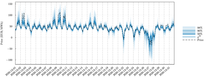
Figure 5: Example of electricity price probabilistic forecasts. Figure plots hourly forecasts for a month of December 2020, predicted by DistrNN.

We provide the hyper-optimisation results that precede the following out-of-sample evaluation in the Appendix A in Figures A2 and A3. The figures show the values of the validation losses of the forward rolling scheme and the corresponding CRPS values of the out-of-sample predictions, and other figures show the values of the hyperparameters selected for the forward rolling scheme specifically for each hour.

5.1  Ouf-of-sample evaluation

Table 2 gives an overview of the results for all models considered, both in point and probabilistic angles. In terms of CRPS loss, the lowest loss value of DistrNN, 1.3669, is about $17\%$ less than the second lowest LEAR-QRA, 1.6497. The accuracy of the LEAR-based quantile regression models, QRA and QRM, is similar. We also observe evidence of better accuracy of DistrNN than LEAR-QRA(QRM) models in the columns of unconditional coverage of prediction intervals. For all three interval sizes, 50%, 90% and 98%, DistrNN reports occurrence rates closest to the nominal values, i.e. the most reliable coverage of prediction intervals. Both LEAR-QRA and LEAR-QRM show larger distances to the nominal value and the occurrence rates are all lower than the nominal $\alpha$s, meaning that the quantile regression methods underestimate the size of the prediction intervals. For DistrNN, this is true for 50% and 90%, although the difference for the latter is less than 1%. The 98%-coverage is matches by DistrNN almost ideally.

We further observe that DistrNN has the lowest MAE and RMSE for point forecasts. Even, the distributional models provide medians, $\widehat{q}^{0.50}$, of probability forecasts, the results are better than the LEAR-Avg optimizing for the mean.

	point			probabilistic
	MAE	RMSE		CRPS		50%-cov	90%-cov	98%-cov
Naive	9.2559	14.2027		3.3409		0.3509	0.6965	0.7915
LEAR-Avg	4.4655	6.7939		-		-	-	-
LEAR-QRM	4.3848	6.7547		1.7048		0.4272	0.8318	0.9348
LEAR-QRA	4.3230	6.6908		1.6497		0.4329	0.8432	0.9577
DistrNN	3.7507	6.3119		1.3669		0.4558	0.8800	0.9792

Table 2: Quantitative results. Point (median) and probabilistic accuracy results. For MAE, RMSE, and CRPS measures lower $\implies$ better, for $\alpha$-coverage measure closer to nominal % coverage $\implies$ better. Colours highlight differences in values from red to green are from the worst to the best.

Figure 6 breaks down the CRPS results from Table 2 into individual quantile losses corresponding to the average of $QL_{\alpha}$ for the OOS period. We see that the DistrNN quantile loss is the lowest for all probability levels. The difference between the losses is negative for all $\alpha$s. This supports that the loss of DistrNN is lower than that of LEAR-QRA.

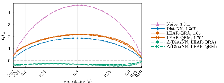
Figure 6: Continuous probability score between models for $\alpha=\{0.01,\dots,0.99\}$ probability levels. Labels in the legend provide the average CRPS of models’ results. Differences between DistrNN and LEAR-QRA(M) are dashed.

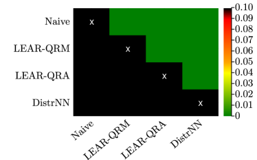
Figure 7: P-values of Diebold-Mariano tests with $\mathcal{H}_{0}:$ Loss of model on y-axis is better than loss of model on x-axis. It depicts p-values for each pair of models. In a cell where the colour is other than black, the model on the x-axis is significantly better than one on the y-axis. When cell is black the p-value is greater than 10%.

In Figure 7 we show the DM test results for the multivariate loss between models. In other words, the overall accuracy between pairs of all models is tested as the sum of the absolute CRPS loss over 24 hours, $L_{m}$, within for the OOS period. The DM test suggests that we reject the null hypothesis that LEAR-QRA is statically better than DistrNN and accept the alternative that DistrNN has significantly better accuracy of probabilistic prediction. In parallel, we do not reject the null that DistrNN has better accuracy than LEAR-QRA. Furthermore, as expected, we see that both LEAR-QRA and DistrNN have statistically better accuracy than the naive predictions.

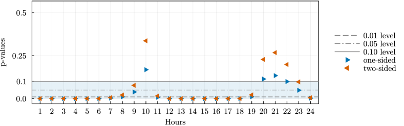
Figure 8: P-values of two Diebold-Mariano tests disaggregated by hours. One-sided test $\mathcal{H}_{0}:$ Loss of LEAR-QRA is better than loss of DistrNN. Two-sided test $\mathcal{H}_{0}:$ Losses of both models are not different.

Finally, in Figure 8 we show the p-values of the Diebold-Mariano test for each hour separately. Above, we have shown that DistrNN provides better accuracy than other models when considering total daily losses. This next result provides an insight into the importance of performance disaggregated by hour. Figure 8 shows that DistrNN has significantly better accuracies than LEAR-QRA for most hours (21 hours) at the 10% probability level, with the three insignificant hours not far from significance. Furthermore, for 16 hours, we reject both one- and two-sided null hypotheses at the 1% significance level.

Note that our CRPS values differ from Marcjasz et al. (2023). To begin with, we do not utilise an ensemble method that combines OOS runs across various hyper-optimization customisations. In contrast, Marcjasz et al. (2023) conducted 4 such runs for both Normal and Johnson’s SU distributions. We obtain single (hyper-optimised) models for the above setup, which exhibit a lower CRPS compared to any of the 8 single hyperparameter set-based models in that study. Since their study confirms that an ensemble of models results in performance gains, we assume that this is also applicable to DistrNN.

The authors use a larger hyperparameter set of 2048 compared to 60 in our setting. The number of searches is also increased by the fact that Marcjasz et al. (2023) manually turn on and off input features, and they also use parameter regularisation in training as dropout and $L_{2}$-norm. In this sense, we use dropout and AdamW learning algorithms to regularise, where the latter mimics $L_{2}$ norm regularisation. In addition, for computational reasons, we limit the number of neurons in the network layers to be between 32 and 384, as opposed to the maximum size of 1024. Comparing the computational cost of the approaches is not straightforward, although the times of both are similar, DistrNN is narrower in this paper and has fewer values in the output layer, it needs to run separately for all 24 hours of a day. Compared to Marcjasz et al. (2023) whose output layer is for one day and all 24 hours using a wider neural network.

Berrisch and Ziel (2023) further improve the results of Marcjasz et al. (2023) with their technique of CRPS learning on already provided OOS results of different models. They provide how to average such results to get a more accurate ensemble average. We do not compete with these results, as the technique can be applied equally well to our DistrNN results.

We do not restrict the reader to taking these results as definitive or to using our approach only as a feed-forward neural network. There may be potential accuracy and performance benefits if the distributional network is recurrent, convolutional, temporal-attentional, and many others. This also opens up space for further analysis, taking into account parsimony and computational cost. Figure A3 in the appendix shows a comparison of the most chosen number of hidden nodes and the most preferred activation function.

5.2  Software and computational time

In recent years, the use of software, particularly in econometrics, has developed rapidly and enormously. We provide a Julia (Bezanson et al., 2012) code that replicates our results and also serves as an example of how to use environments other than languages, such as python or R. The exercise uses the Flux.jl package (Innes et al., 2018) and the results can be replicated using examples at https://github.com/luboshanus/DistrNNEnergy.jl, which may make the process easier for those using Julia to predict (energy) time series.

The complete estimation process of DistrNN, involving the hyper-optimisation search and a forward rolling window scheme across 24 hours, 736 OOS observations, 60 hyperparameter sets, 7 folds, 8 ensembles, using 1000 epochs and 64 mini-batch size, entails the estimation of 10080 (24*60*7) and 141312 (24*736*8) networks. Therefore, obtaining an out-of-sample prediction can take approximately 24 to 48 hours, depending on the number of ensembles (2-8). We distribute the hyper-optimisation and rolling estimation tasks over 60 CPU cores. The complete estimation of LEAR-QRA(QRM) in Julia takes about 15 minutes when distributed over 15 CPU cores.

6  Conclusion

This paper proposes a novel machine learning approach to probabilistic forecasting of hourly day-ahead electricity prices. Compared to the state-of-the-art frameworks in the (probabilistic) electricity price forecasting literature, our model provides more accurate forecasts. This is mainly due to the fact that it does not rely on restrictive model assumptions and allows for non-Gaussian, heavy-tailed data and their non-linear interactions. By relaxing the assumption on the distribution family of the time series, our distributional neural network explores the data fully. We also provide an efficient computational package that can be used by researchers.

Appendix for

“Learning Probability Distributions of Day-Ahead Electricity Prices”

A  Additional tables and figures

A.1  Point forecasts

If taken into accounts means and medians from the models and distribution, we provide results of DM test of mean absolute errors between models. The average of point forecasts of different calibration windows performs best in this case, then it is the DistrNN median, see Figure A1.

Figure A1: P-values of Diebold-Mariano tests for MAE of $\widehat{q}^{0.50}$ or $\bar{y}_{t}$ in $L_{m}$ with $\mathcal{H}_{0}:$ Loss of model on y-axis is better than loss of model on x-axis. Where the colour is other than black, the model on the x-axis is significantly better than one on the y-axis.

A.2  Hyper-optimization results

Here we provide figures documenting training and validation process, as results of all validation losses related to forward rolling training scheme, Figure A2, , and the selection of best parameters sets, see Figure A3.

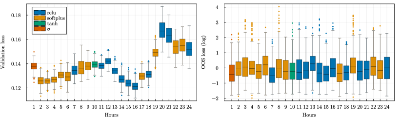
Figure A2: Rolling scheme results of validation losses and out-of-sample losses for 24 hours. Figure (left) shows evolution of validation losses (binary cross-entropy) in comparison to out-of-sample loss (CRPS) values for each hour. The colours show which activation function has been selected by the hyper-optimization for given hour. Every histogram contains 554 (+182 discarded) values $times$ 4 of those considered for ensembles.

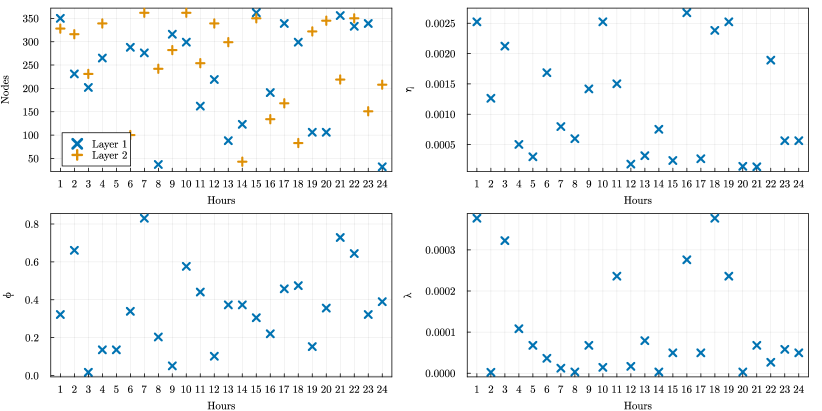
Figure A3: Hyper-optimisation results. The figures show the values of the parameters that make up the best sets used to re-learn/re-calibrate the neural networks for each hour. Together with these parameters, the hyper-optimisation selects the activation function, and the selected ones are shown in colour in the figure A2.

B  CDF interpolation

The Fritsch–Carlson monotonic cubic interpolation (Fritsch and Carlson, 1980) provides a monotonically increasing CDF with range $[0,1]$ when applied to CDF estimates on a finite grid.

Suppose we have CDF $F(y)$ defined at points $(y_{k},F(y_{k}))$ for $k=1,\dots,K,$ where $F(y_{0})=0$ and $F(y_{K})=1$. We presume that $y_{k}<y_{k+1}$ and $F(y_{k})<F(y_{k+1})$ for all $k=0,\dots,K-1,$ which is warranted by continuity of returns and construction of the estimated distribution. First, we compute slopes of the secant lines as $\Delta_{k}=(F(y_{k+1})-F(y_{k})))/(y_{k+1}-y_{k})$ for $k=1,\dots,K-1,$ and then the tangents at every data point as $m_{1}=\Delta_{1}$, $m_{k}=\frac{1}{2}(\Delta_{k-1}+\Delta_{k})$ for $k=2,\dots,K-1$, and $m_{K}=\Delta_{K-1}.$ Let $\alpha_{k}=m_{k}/\Delta_{k}$ and $\beta_{k}=m_{k+1}/\Delta_{k}$ for $k=1,\dots,K-1$. If $\alpha_{k}^{2}+\beta_{k}^{2}>9$ for some $k=1,\dots,K-1,$ then we set $m_{k}=\alpha_{k}\alpha_{k}\Delta_{k}$ and $m_{k+1}=\alpha_{k}\beta_{k}\Delta_{k},$ with $\alpha_{k}=3(\alpha_{k}^{2}+\beta_{k}^{2})^{-1/2}$. Finally, the cubic Hermite spline is applied: for any $y\in[y_{k},y_{k+1}]$ for some $k=0,\dots,K-1,$ we evaluate $F(y)$ as

$$F(y)=(2t^{3}-3t^{2}+1)F(y_{k})+(t^{3}-2t^{2}+t)hy_{k}+(-2t^{3}+3t^{2})F(y_{k+1})+(t^{3}-t^{2})hm_{k+1},$$

where $h=y_{k+1}-y_{k}$ and $t=(y-y_{k})/h.$

References

- Anatolyev and Baruník (2019) Anatolyev, S. and J. Baruník (2019). Forecasting dynamic return distributions based on ordered binary choice. International Journal of Forecasting 35(3), 823–835.
- Berrisch and Ziel (2023) Berrisch, J. and F. Ziel (2023). Multivariate probabilistic crps learning with an application to day-ahead electricity prices. arXiv preprint arXiv:2303.10019.
- Bezanson et al. (2012) Bezanson, J., S. Karpinski, V. B. Shah, and A. Edelman (2012). Julia: A fast dynamic language for technical computing. arXiv preprint arXiv:1209.5145.
- Bianchi et al. (2020) Bianchi, D., M. Büchner, and A. Tamoni (2020). Bond risk premia with machine learning. Review of Financial Studies (forthcoming).
- Box et al. (1987) Box, G. E., N. R. Draper, et al. (1987). Empirical model-building and response surfaces, Volume 424. Wiley New York.
- Box et al. (2015) Box, G. E., G. M. Jenkins, G. C. Reinsel, and G. M. Ljung (2015). Time series analysis: forecasting and control. John Wiley & Sons.
- Bunn et al. (2016) Bunn, D., A. Andresen, D. Chen, and S. Westgaard (2016). Analysis and forecasting of electricty price risks with quantile factor models. The Energy Journal 37(1).
- Chernozhukov et al. (2013) Chernozhukov, V., I. Fernández-Val, and B. Melly (2013). Inference on counterfactual distributions. Econometrica 81(6), 2205–2268.
- Clements et al. (2008) Clements, M. P., A. B. Galvão, and J. H. Kim (2008). Quantile forecasts of daily exchange rate returns from forecasts of realized volatility. Journal of Empirical Finance 15(4), 729–750.
- Coulombe et al. (2020) Coulombe, P. G., M. Leroux, D. Stevanovic, and S. Surprenant (2020). How is machine learning useful for macroeconomic forecasting? arXiv preprint arXiv:2008.12477.
- Diebold (2021) Diebold, F. X. (2021). What’s the big idea? big data and its origins. Significance 19, 36–37.
- Diebold and Mariano (1995) Diebold, F. X. and R. S. Mariano (1995). Comparing predictive accuracy. Journal of Business & Economic Statistics 13(3).
- Efron et al. (2004) Efron, B., T. Hastie, I. Johnstone, and R. Tibshirani (2004). Least angle regression.
- Feng et al. (2018) Feng, G., J. He, and N. G. Polson (2018). Deep learning for predicting asset returns. arXiv preprint arXiv:1804.09314.
- Foresi and Peracchi (1995) Foresi, S. and F. Peracchi (1995). The conditional distribution of excess returns: An empirical analysis. Journal of the American Statistical Association 90(430), 451–466.
- Fritsch and Carlson (1980) Fritsch, F. N. and R. E. Carlson (1980). Monotone piecewise cubic interpolation. SIAM Journal on Numerical Analysis 17(2).
- Gneiting and Raftery (2007) Gneiting, T. and A. E. Raftery (2007). Strictly proper scoring rules, prediction, and estimation. Journal of the American statistical Association 102(477), 359–378.
- Gu et al. (2020) Gu, S., B. Kelly, and D. Xiu (2020). Empirical asset pricing via machine learning. The Review of Financial Studies 33(5), 2223–2273.
- Heaton et al. (2017) Heaton, J. B., N. G. Polson, and J. H. Witte (2017). Deep learning for finance: deep portfolios. Applied Stochastic Models in Business and Industry 33(1), 3–12.
- Hyndman et al. (2008) Hyndman, R., A. B. Koehler, J. K. Ord, and R. D. Snyder (2008). Forecasting with exponential smoothing: the state space approach. Springer Science & Business Media.
- Innes et al. (2018) Innes, M., E. Saba, K. Fischer, D. Gandhi, M. C. Rudilosso, N. M. Joy, T. Karmali, A. Pal, and V. Shah (2018). Fashionable modelling with flux. CoRR abs/1811.01457.
- Israel et al. (2020) Israel, R., B. T. Kelly, and T. J. Moskowitz (2020). Can machines’ learn’finance? Available at SSRN 3624052.
- Iworiso and Vrontos (2020) Iworiso, J. and S. Vrontos (2020). On the directional predictability of equity premium using machine learning techniques. Journal of Forecasting 39(3), 449–469.
- Kingma and Ba (2014) Kingma, D. P. and J. Ba (2014). Adam: A method for stochastic optimization. arXiv preprint arXiv:1412.6980.
- Klein et al. (2023) Klein, N., M. S. Smith, and D. J. Nott (2023). Deep distributional time series models and the probabilistic forecasting of intraday electricity prices. Journal of Applied Econometrics.
- Koenker and Bassett Jr (1978) Koenker, R. and G. Bassett Jr (1978). Regression quantiles. Econometrica: journal of the Econometric Society, 33–50.
- Kuan and White (1994) Kuan, C.-M. and H. White (1994). Artificial neural networks: An econometric perspective. Econometric reviews 13(1), 1–91.
- Lago et al. (2021) Lago, J., G. Marcjasz, B. De Schutter, and R. Weron (2021). Forecasting day-ahead electricity prices: A review of state-of-the-art algorithms, best practices and an open-access benchmark. Applied Energy 293, 116983.
- Lago et al. (2021) Lago, J., G. Marcjasz, B. De Schutter, and R. Weron (2021). Forecasting day-ahead electricity prices: A review of state-of-the-art algorithms, best practices and an open-access benchmark. Applied Energy 293, 116983.
- Lago et al. (2021) Lago, J., G. Marcjasz, B. D. Schutter, and R. Weron (2021, July). EPFTOOLBOX: The first open-access PYTHON library for driving research in electricity price forecasting (EPF). WORMS Software (WORking papers in Management Science Software), Department of Operations Research and Business Intelligence, Wroclaw University of Science and Technology.
- Lehna et al. (2022) Lehna, M., F. Scheller, and H. Herwartz (2022). Forecasting day-ahead electricity prices: A comparison of time series and neural network models taking external regressors into account. Energy Economics 106, 105742.
- Liu et al. (2017) Liu, B., J. Nowotarski, T. Hong, and R. Weron (2017). Probabilistic load forecasting via quantile regression averaging on sister forecasts. IEEE Transactions on Smart Grid 8(2), 730–737.
- Loshchilov and Hutter (2019) Loshchilov, I. and F. Hutter (2019). Decoupled weight decay regularization. arXiv preprint arXiv:1711.05101.
- Maciejowska (2020) Maciejowska, K. (2020). Assessing the impact of renewable energy sources on the electricity price level and variability–a quantile regression approach. Energy Economics 85, 104532.
- Maciejowska et al. (2016) Maciejowska, K., J. Nowotarski, and R. Weron (2016). Probabilistic forecasting of electricity spot prices using factor quantile regression averaging. International Journal of Forecasting 32(3), 957–965.
- Marcjasz et al. (2023) Marcjasz, G., M. Narajewski, R. Weron, and F. Ziel (2023). Distributional neural networks for electricity price forecasting. Energy Economics 125, 106843.
- Marcjasz et al. (2020) Marcjasz, G., B. Uniejewski, and R. Weron (2020). Probabilistic electricity price forecasting with narx networks: Combine point or probabilistic forecasts? International Journal of Forecasting 36(2), 466–479.
- Mashlakov et al. (2021) Mashlakov, A., T. Kuronen, L. Lensu, A. Kaarna, and S. Honkapuro (2021). Assessing the performance of deep learning models for multivariate probabilistic energy forecasting. Applied Energy 285, 116405.
- Mpfumali et al. (2019) Mpfumali, P., C. Sigauke, A. Bere, and S. Mulaudzi (2019). Day ahead hourly global horizontal irradiance forecasting—application to south african data. Energies 12(18).
- Mullainathan and Spiess (2017) Mullainathan, S. and J. Spiess (2017). Machine learning: an applied econometric approach. Journal of Economic Perspectives 31(2), 87–106.
- Narajewski and Ziel (2020) Narajewski, M. and F. Ziel (2020). Econometric modelling and forecasting of intraday electricity prices. Journal of Commodity Markets 19, 100107.
- Nowotarski and Weron (2015) Nowotarski, J. and R. Weron (2015). Computing electricity spot price prediction intervals using quantile regression and forecast averaging. Computational Statistics 30(3), 791–803.
- Nowotarski and Weron (2018) Nowotarski, J. and R. Weron (2018). Recent advances in electricity price forecasting: A review of probabilistic forecasting. Renewable and Sustainable Energy Reviews 81, 1548–1568.
- Petropoulos et al. (2022) Petropoulos, F., D. Apiletti, V. Assimakopoulos, M. Z. Babai, D. K. Barrow, S. B. Taieb, C. Bergmeir, R. J. Bessa, J. Bijak, J. E. Boylan, et al. (2022). Forecasting: theory and practice. International Journal of Forecasting 38(3), 705–871.
- Salinas et al. (2020) Salinas, D., V. Flunkert, J. Gasthaus, and T. Januschowski (2020). Deepar: Probabilistic forecasting with autoregressive recurrent networks. International Journal of Forecasting 36(3), 1181–1191.
- Serafin et al. (2019) Serafin, T., B. Uniejewski, and R. Weron (2019). Averaging predictive distributions across calibration windows for day-ahead electricity price forecasting. Energies 12(13), 2561.
- Sirignano et al. (2016) Sirignano, J., A. Sadhwani, and K. Giesecke (2016). Deep learning for mortgage risk. arXiv preprint arXiv:1607.02470.
- Srivastava et al. (2014) Srivastava, N., G. Hinton, A. Krizhevsky, I. Sutskever, and R. Salakhutdinov (2014). Dropout: a simple way to prevent neural networks from overfitting. The Journal of Machine Learning Research 15(1), 1929–1958.
- Tibshirani (1996) Tibshirani, R. (1996). Regression shrinkage and selection via the lasso. Journal of the Royal Statistical Society Series B: Statistical Methodology 58(1), 267–288.
- Tobek and Hronec (2020) Tobek, O. and M. Hronec (2020). Does it pay to follow anomalies research? machine learning approach with international evidence. Journal of Financial Markets, 100588.
- Uniejewski et al. (2019) Uniejewski, B., G. Marcjasz, and R. Weron (2019). On the importance of the long-term seasonal component in day-ahead electricity price forecasting: Part ii — probabilistic forecasting. Energy Economics 79, 171–182. Energy Markets Dynamics in a Changing Environment.
- Uniejewski et al. (2016) Uniejewski, B., J. Nowotarski, and R. Weron (2016). Automated variable selection and shrinkage for day-ahead electricity price forecasting. Energies 9(8).
- Uniejewski et al. (2018) Uniejewski, B., R. Weron, and F. Ziel (2018). Variance stabilizing transformations for electricity spot price forecasting. IEEE Transactions on Power Systems 33(2), 2219–2229.
- Weron (2014) Weron, R. (2014). Electricity price forecasting: A review of the state-of-the-art with a look into the future. International Journal of Forecasting 30(4), 1030–1081.
- Zhang et al. (2022) Zhang, F., H. Fleyeh, and C. Bales (2022). A hybrid model based on bidirectional long short-term memory neural network and catboost for short-term electricity spot price forecasting. Journal of the Operational Research Society 73(2), 301–325.
- Zhang et al. (2018) Zhang, W., H. Quan, and D. Srinivasan (2018). Parallel and reliable probabilistic load forecasting via quantile regression forest and quantile determination. Energy 160, 810–819.
- Ziel and Weron (2018) Ziel, F. and R. Weron (2018). Day-ahead electricity price forecasting with high-dimensional structures: Univariate vs. multivariate modeling frameworks. Energy Economics 70, 396–420.