Graph-based Simultaneous Localization and Bias Tracking

Abstract

We present a factor graph formulation and particle-based sum-product algorithm for robust localization and tracking in multipath-prone environments. The proposed sequential algorithm jointly estimates the mobile agent’s position together with a time-varying number of multipath components. The MPCs are represented by “delay biases” corresponding to the offset between line-of-sight (LOS) component delay and the respective delays of all detectable MPCs. The delay biases of the MPCs capture the geometric features of the propagation environment with respect to the mobile agent. Therefore, they can provide position-related information contained in the MPCs without explicitly building a map of the environment. We demonstrate that the position-related information enables the algorithm to provide high-accuracy position estimates even in fully obstructed line-of-sight (OLOS) situations. Using simulated and real measurements in different scenarios we demonstrate the proposed algorithm to significantly outperform state-of-the-art multipath-aided tracking algorithms and show that the performance of our algorithm constantly attains the posterior Cramér-Rao lower bound (P-CRLB). Furthermore, we demonstrate the implicit capability of the proposed method to identify unreliable measurements and, thus, to mitigate lost tracks.

I Introduction

Localization of mobile agents using radio signals is still a challenging task in indoor or urban scenarios[1, 2]. Here, the environment is characterized by strong multipath propagation (commonly referred to as “ non-line-of-sight (NLOS) propagation”) and frequent OLOS situations, which can prevent the correct extraction of the information contained in the LOS component (see Fig. 1). There exist many safety and security-critical applications, such as autonomous driving [3], or medical services [4], where robustness of the position estimate is of critical importance.

I-A State-of-the-Art Methods

New localization and tracking approaches within the context of 6G networks take advantage of large measurement apertures as provided by ultra wide band (UWB) systems [5, 6] and the large number of antennas in mmWave systems [7], allowing to resolve the received radio signal into a superposition of a finite number of specular MPCs [5, 8, 9]. These approaches mitigate the effect of multipath propagation [10] aiming to obtain unbiased estimates of the LOS component [9, 5, 11] or even take advantage of MPCs by exploiting inherent position information, turning multipath from impairment to an asset [12, 13, 14]. Prominent examples of such approaches are multipath-based SLAM (MP-SLAM) methods [14, 15, 12, 16] that estimate MPCs and associate them to virtual anchors representing the locations of the mirror images of anchors on reflecting surfaces [17]. The locations of VAs are estimated jointly with the position of the mobile agent. This way, MP-SLAM can provide high-accuracy position estimates, even in OLOS situations [18]. However, it requires specular, resolved MPCs generated by environments consistent with the VA model, i.e., flat surfaces of sufficient extend[17]. This is why the method introduced in [19] performs MP-SLAM considering antenna dispersion and diffuse / non-resolvable MPCs at the cost of increased problem complexity. Similarly, the approximate method introduced in [20, 18] exploits the positional information of MPCs using a low-complexity model featuring a single bias to a stochastically modeled multipath “cluster” to perform robust positioning and tracking. Although MP-SLAM can be straightforwardly extended to three dimensions[21], this significantly increases the complexity of the inference model and, thus, complicates the numerical representation. Furthermore, in scenarios where the number of detectable VAs is low (sparse information), geometric ambiguity can lead to a multimodal state distribution and, thus, cause the algorithm to follow wrong modes [22].

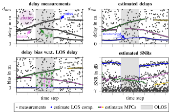
Figure 1: In OLOS situations the LOS path is reconstructed using the position-related information contained in the delay biases of all detected MPCs. The delay biases as well as their SNRs are jointly estimated together with the agent’s state. The estimation problem is complicated by false alarms (clutter), missed detections (miss), object birth (birth), and object death (death).

Machine learning methods avoid model-based representations, relying on data to capture details of the actual environment. Yet, applying deep machine learning to complex inference tasks is not straightforward. Early approaches for learning-aided multipath-based positioning extract specific features from the radio channel, applying model-agnostic supervised regression methods on these features [23, 11]. While these approaches potentially provide high accuracy estimates at low computational demand (after training), they suffer from their dependence on a large representative database and can fail in scenarios that are not sufficiently represented by the training data. This is why recent algorithms use deep learning and auto encoding-based methods, directly operating on the received radio signal [24, 25, 26] and hybrid, physics-informed learning models [27, 24, 28] to reduce the dependence on training data.

Bayesian inference leveraging graphical models provides a powerful and flexible means that has been widely used in applications like multipath-based localization [12, 14, 15, 16, 20], multiobject-tracking [29, 30, 31], and parametric channel tracking [32]. These applications pose common challenges such as uncertainties beyond Gaussian noise (missed detections and clutter), an uncertain origin of measurements, and unknown and time-varying numbers of objects to be localized and tracked. As the measurement models of these applications are non-linear, most methods typically rely on particle-based implementations or linearization [33, 34]. Similarly, the probabilistic data association (PDA) algorithm [29, 35] represents a low-complexity Bayesian method for robust localization and tracking with extension to multiple-sensors PDA [36] and amplitude-information (AIPDA) [37, 15]. All these methods can be categorized as “two-step approaches”, in the sense that they do not operate on the received sampled radio signal, but use extracted measurements provided by a preprocessing step, providing a high level of flexibility and a significant reduction of computational complexity. In contrast, “direct positioning approaches” such as [38, 39] directly exploit the received sampled signal, which can lead to a better detectability of low- signal-to-noise-ratio (SNR) features, yet, they are computationally very demanding.

I-B Contributions

The problem studied in this paper can be summarized as follows.

Estimate the time-varying location of a mobile agent using LOS propagation and NLOS propagation of radio signals.

We propose a particle-based algorithm for robust localization and tracking that estimates the state of a mobile agent by utilizing the position-related information contained in the LOS component as well as in multipath components (MPCs) of multiple sensors (anchors). Similar to other “two-step approaches”, it uses MPC delays and corresponding amplitude measurements provided by a snapshot-based parametric channel estimation and detection algorithm (CEDA). The proposed algorithm performs joint probabilistic data association and sequential estimation [30, 14] of a mobile agent state together with all parameters of a time-varying number of potential bias objects (PBOs), using message passing by means of the sum-product algorithm (SPA) on a factor graph [40]. potential bias objects contain a state representation of “delay biases”, denoting the delay difference between the LOS component and the respective MPCs, as well as a binary variable denoting the existence of the respective MPCs. This model enables the algorithm to utilize the position information contained in the MPCs without building an explicit representation of an environment map [12, 14] in order to support the estimation of the agent state (see Fig. 1). This allows the algorithm to operate reliably in challenging environments, characterized by strong multipath propagation and temporary OLOS situations without using any prior information (no training data are needed). The key contributions of this paper are as follows.

• We introduce a Bayesian model for MPC-aided localization and tracking of the position by sequential inference of a possibly time-varying number of PBOs.

• We present an SPA based on the factor graph representation of the estimation problem where the PBO states are estimated jointly and sequentially, demonstrating that the information contained in PBOs dramatically increases the performance in OLOS situations. Also, we demonstrate the capability of the proposed method to identify unreliable estimates using the existence probability of the PBOs.

• We compare the proposed SPA to other state-of-the-art algorithms for MPC-aided localization and tracking as well as to the P-CRLB [41] using both synthetic and real radio measurements. Specifically, we compare to our robust positioning method from [18], and to the MP-SLAM method presented in [14, 15]. For synthetic measurements, we also compare to the learning-based methods presented in [11] and [28].

This work advances over the preliminary account of our conference publication [42] by (i) presenting a detailed derivation of the proposed SPA and its particle-based implementation, (ii) thoroughly analyzing the geometric relations underlying the proposed model, (iii) presenting a comprehensive numerical analysis of the algorithm performance, (iv) comparing to the MP-SLAM algorithm presented in [14, 15], (v) comparing to the learning-based methods presented in [11] and [28, 25], (vi) validating the performance of the proposed algorithm using real radio measurements and, (vii) demonstrating the implicit capability of the proposed method to identify unreliable measurements.

Notations and Definitions

Column vectors and matrices are denoted by boldface lowercase and uppercase letters. Random variables are displayed in san serif, upright font, e.g., $\mathsfbr{x}$ and $\bm{\mathsfbr{x}}$ and their realizations in serif, italic font, e.g. $x$. $f({x})$ and $p({x})$ denote, respectively, the probability density function (PDF) or probability mass function (PMF) of a continuous or discrete random variable $\mathsfbr{x}$ (these are short notations for $f{x}({x})$ or $p{x}({x})$). $(\cdot)^{\mathrm{T}}$, $(\cdot)^{\ast}$, and $(\cdot)^{\text{H}}$ denote matrix transpose, complex conjugation and Hermitian transpose, respectively. $\lVert\cdot\rVert$ is the Euclidean norm. $|\cdot|$ represents the cardinality of a set. $\mathrm{diag}\{\bm{x}\}$ denotes a diagonal matrix with entries in $\bm{x}$. $\bm{I}_{[\cdot]}$ is an identity matrix of dimension given in the subscript. $[\bm{X}]_{n,n}$ denotes the $n$th diagonal entry of $\bm{X}$. Furthermore, ${1}_{\mathbb{A}}(\bm{x})$ denotes the indicator function that is ${1}_{\mathbb{A}}(\bm{x})=1$ if $\bm{x}\in\mathbb{A}$ and 0 otherwise, for $\mathbb{A}$ being an arbitrary set and $\mathbb{R}^{\text{+}}$ is the set of positive real numbers. We predefine the following PDFs with respect to (w.r.t.) $\mathsfbr{x}$: The truncated Gaussian PDF is

$$f_{\text{TN}}(x;\mu,\sigma,\lambda)=\frac{1}{Q(\frac{\lambda-\mu}{\sigma})\sqrt{2\pi}\sigma}e^{\frac{-(x-\mu)^{2}}{2\,\sigma^{2}}}{1}_{\mathbb{R}^{\text{+}}}(x-\lambda)$$ (1)

with mean $\mu$, standard deviation $\sigma$, truncation threshold $\lambda$ and $Q(\cdot)$ denoting the Q-function [43]. Accordingly, the Gaussian PDF is $f_{\text{N}}(x;\mu,\sigma)=f_{\text{TN}}(x;\mu,\sigma,\text{-}\hskip 0.5pt\infty)$. The truncated Rician PDF is [44, Ch. 1.6.7]

$$f_{\text{TRice}}(x;s,u,\lambda)=\frac{1}{Q_{1}(\frac{u}{s},\frac{\lambda}{s})}\frac{x}{s^{2}}e^{\frac{-(x^{2}+u^{2})}{2\,s^{2}}}I_{0}(\frac{x\,u}{s^{2}}){1}_{\mathbb{R}^{\text{+}}}(x-\lambda)$$ (2)

with non-centrality parameter $u$, scale parameter $s$ and truncation threshold $\lambda$. $I_{0}(\cdot)$ is the 0th-order modified first-kind Bessel function and $Q_{1}(\cdot,\cdot)$ denotes the Marcum Q-function [43]. The truncated Rayleigh PDF is [44, Ch. 1.6.7]

$$f_{\text{TRayl}}(x;s,\lambda)=\frac{x}{s^{2}}\,e^{\frac{-(x^{2}-\lambda^{2})}{2\,s^{2}}}{1}_{\mathbb{R}^{\text{+}}}(x-\lambda)$$ (3)

with scale parameter $s$ and truncation threshold $\lambda$. This formula corresponds to the so-called Swirling I model[44]. Finally, we define the uniform PDF $f_{\mathrm{U}}(x;a,b)=1/(b-a){1}_{[a,b]}(x)$ and the uniform PMF $p_{\mathrm{UD}}(x;\mathcal{X})=1/|\mathcal{X}|{1}_{\mathcal{X}}(x)$.

II Geometrical Relations

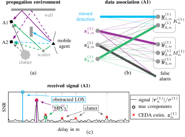
Figure 2: Graphical overview of (a) an exemplary radio propagation environment, (b) joint probabilistic data association using measurements of anchor A1, and (c) the received signal vector of anchor A1.

We consider a mobile agent equipped with a single antenna that moves along an unknown trajectory. At each time $n$, the mobile agent at position ${\bm{p}}_{n}$ transmits a radio signal and each anchor $j\in\{1,\hskip 0.5pt...\hskip 0.5pt,J\}$ equipped with a single antenna at anchor position $\bm{p}_{\text{A}}^{(j)}=[p_{\text{Ax}}^{(j)}\;p_{\text{Ay}}^{(j)}]^{\text{T}}$ acts as a receiver (see Fig. 2a). The Euclidean distance between mobile agent at time $n$ and anchor $j$ (i.e., the LOS path) is given as $\lVert\bm{p}_{n}-\bm{p}_{\text{A}}^{(j)}\rVert$. Specular reflections of radio signals on flat surfaces (planar walls, floor, ceiling,…) can be described by VAs that are mirror images of the anchors [17, 45]. Similarly, point scatters are described by the sum of their distance w.r.t. the agent ${\bm{p}}_{n}$ and their distance w.r.t. the anchor $\bm{p}_{\text{A}}^{(j)}$ [12], where the latter is constant over time $n$. The “distance bias” $b_{l,n}^{(j)}$ corresponding to the $l$-th MPC at time $n$ and for anchor $j$, caused by one of the discussed phenomena, is given as

$$b_{l,n}^{(j)}(\bm{p}_{n})=\lVert\bm{p}_{n}-\bm{p}_{\text{MPC}\hskip 0.5ptl}^{(j)}\rVert-\lVert\bm{p}_{n}-\bm{p}_{\text{A}}^{(j)}\rVert+c_{\text{MPC}\hskip 0.5ptl}^{(j)}$$ (4)

with $\bm{p}_{\text{MPC}\hskip 0.5ptl}^{(j)}$ being the position corresponding to the current VA or point scatter and $c_{\text{MPC}\hskip 0.5ptl}^{(j)}$ being an offset which is constant over time $n$ and equals zero for VAs or $\lVert\bm{p}_{\text{A}}^{(j)}-\bm{p}_{\text{MPC}\hskip 0.5ptl}^{(j)}\rVert$ for point scatters, respectively. In this work we are interested to model the temporal evolution of the distance bias. To this end, we consider the bias difference, denoted as

$$\Delta b_{l,n}^{(j)}(\bm{p}_{n},\bm{p}_{n-1})\triangleq b_{l,n}^{(j)}(\bm{p}_{n})-b_{l,n-1}^{(j)}(\bm{p}_{n-1})\,$$ (5)

which, in general, is a nonlinear function of $\bm{p}_{n}$ and $\bm{p}_{n-1}$. However, if the distance between agent and anchor $\lVert\bm{p}_{n}-\bm{p}_{\text{A}}^{(j)}\rVert$ is large compared to the agent movement $\lVert\bm{p}_{n}-\bm{p}_{n-1}\rVert$, the bias difference is well approximated as

$$\Delta b_{l,n}^{(j)}(\bm{p}_{n},\bm{p}_{n-1})\approx(\bm{p}_{n}-\bm{p}_{n-1})^{\text{T}}(\bm{e}_{\text{MPC}\hskip 0.5ptl,n}^{(j)}-\bm{e}_{\text{A}\hskip 0.5ptn}^{(j)})\,$$ (6)

where $\bm{e}_{\text{MPC}\hskip 0.5ptl,n}^{(j)}\triangleq(\bm{p}_{n}-\bm{p}_{\text{MPC}\hskip 0.5ptl}^{(j)})/\lVert\bm{p}_{n}-\bm{p}_{\text{MPC}\hskip 0.5ptl}^{(j)}\rVert$ and $\bm{e}_{\text{A}\hskip 0.5ptn}^{(j)}\triangleq(\bm{p}_{n}-\bm{p}_{\text{A}}^{(j)})/\lVert\bm{p}_{n}-\bm{p}_{\text{A}}^{(j)}\rVert$ are unit vectors that point from $\bm{p}_{\text{MPC}\hskip 0.5ptl}^{(j)}$ and $\bm{p}_{\text{A}}^{(j)}$, respectively, in the direction of the mobile agent. Note that this implies the the distances $\lVert\bm{p}_{n}-\bm{p}_{\text{MPC}\hskip 0.5ptl}^{(j)}\rVert$ are also large w.r.t. the agent movement. The approximation used in (6) is known in literature as the far field assumption [46, 47] and is geometrically visualized w.r.t. $\bm{p}_{\text{A}\hskip 0.5ptn}^{(j)}$ in Fig. 3 (but equally applies for $\bm{p}_{\text{MPC}\hskip 0.5ptl}^{(j)}$).

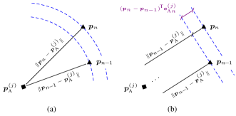
Figure 3: Exact geometry (a) vs. far field assumption (b) w.r.t. $\bm{p}_{\text{A}\hskip 0.5ptn}^{(j)}$.

It is based on the observation that the unit vectors $\bm{e}_{\text{A}\hskip 0.5ptn-1}^{(j)}$ and $\bm{e}_{\text{A}\hskip 0.5ptn}^{(j)}$ or $\bm{e}_{\text{MPC}\hskip 0.5ptl,n-1}^{(j)}$ and $\bm{e}_{\text{MPC}\hskip 0.5ptl,n}^{(j)}$, respectively, are similar. Analyzing (6), we observe that (i) (6) is a linear function w.r.t. the agent positions $\bm{p}_{n}$ and $\bm{p}_{n-1}$, i.e., a locally linear agent movement leads to a locally linear change of the delay bias, (ii) VAs or point scatters, which take a similar angle w.r.t. the agent, i.e., $\bm{e}_{\text{A}\hskip 0.5ptn}^{(j)}\approx\bm{e}_{\text{MPC}\hskip 0.5ptl,n}^{(j)}$, lead to small bias differences $\Delta b_{l,n}^{(j)}(\bm{p}_{n},\bm{p}_{n-1})\approx 0$ even if the agent movement follows a non-linear path (e.g. sudden turns). The proposed method utilizes the above observations by tracking the distance biases $b_{l,n}^{(j)}(\bm{p}_{n})$ to each MPC using a (locally linear) constant velocity model. Thus, the proposed method is exploiting “local” map information.

III Radio Signal Model and Channel Estimation

The received complex baseband signal at the $j$th anchor is sampled $N_{\text{s}}$ times with sampling frequency $f_{\text{s}}=1/T_{\text{s}}$ yielding an observation period of $T=N_{\text{s}}\,T_{\text{s}}$. By stacking the samples, we obtain the discrete-time received signal vector [48, 18]

$$\bm{\mathsfbr{r}}_{n}^{(j)}={\alpha}_{n,1}^{(j)}\bm{s}({\tau}_{n,1}^{(j)})+\sum_{l=2}^{{L}_{n}^{(j)}}{\alpha}_{n,l}^{(j)}\bm{s}({\tau}_{n,l}^{(j)})+\bm{\mathsfbr{n{}}}_{n}^{(j)}$$ (7)

where $\bm{s}(\tau)\triangleq[s(-(N_{\text{s}}-1)\hskip 0.85358ptT_{\text{s}}/2-\tau)\,\,\,\cdots\,\,\,s((N_{\text{s}}-1)\hskip 0.85358ptT_{\text{s}}/2-\tau)]^{\text{T}}\in\mathbb{C}^{N_{\text{s}}\times 1}$ is the discrete-time transmit pulse with delay $\tau$. The first and second terms describe the LOS component and the sum of ${L}_{n}^{(j)}-1$ specular MPCs with their corresponding complex amplitudes ${\alpha}_{n,l}^{(j)}$ and delays ${\tau}_{n,l}^{(j)}$, respectively. The delays are related to respective distances via ${\tau}_{n,l}^{(j)}={d}_{n,l}^{(j)}/\hskip 0.5ptc$ with $c$ being the speed of light. The measurement noise vector $\bm{\mathsfbr{n{}}}_{n}^{(j)}\in\mathbb{C}^{N_{\text{s}}\times 1}$ is a zero-mean, circularly-symmetric complex Gaussian random vector with covariance matrix ${\sigma}^{(j)\hskip 0.5pt2}\bm{I}_{N_{\text{s}}}$ and noise variance is given by ${\sigma}^{(j)\hskip 0.5pt2}={N}_{0}^{(j)}/T_{\text{s}}$. The MPCs arise from reflection by unknown objects, since we assume that no map information is available. The component SNR of each MPC is $\mathrm{SNR}^{(j)}_{n,l}=|{\alpha}^{(j)}_{n,l}|^{2}\lVert\bm{s}({\tau}_{n,l}^{(j)})\rVert^{2}/{\sigma}^{(j)\hskip 0.5pt2}$ and the corresponding normalized amplitude is ${u}^{(j)}_{n,l}\triangleq\mathrm{SNR}^{(j)\hskip 0.5pt\frac{1}{2}}_{n,l}$. We assume time and frequency synchronization between all anchors and the mobile agent. However, our model can be extended to an unsynchronized system similarly as in [12].

III-A Parametric Channel Estimation

By applying a snapshot-based, super-resolution CEDA[49, 50, 48] to the observed discrete signal vector $\bm{r}_{n}^{(j)}$, one obtains, at each time $n$ and anchor $j$, a number of $M_{n}^{(j)}$ measurements denoted by ${\bm{z}^{(j)}_{m,n}}$ with $m\in\{1,\,...\,,M_{n}^{(j)}\}\triangleq\mathcal{M}_{n}^{(j)}$. Each ${\bm{z}^{(j)}_{m,n}}=[{z_{\mathrm{d}}^{(j)}}_{m,n}~{}{z_{\mathrm{u}}^{(j)}}_{m,n}]^{\text{T}}$, representing a potential MPC parameter estimate, contains a distance measurement ${z_{\mathrm{d}}^{(j)}}_{m,n}\in[0,d_{\text{max}}]$ and a normalized amplitude measurement ${z_{\mathrm{u}}^{(j)}}_{m,n}\in[\gamma,\infty)$, where $d_{\text{max}}$ is the maximum possible distance and $\gamma$ is the detection threshold of the CEDA. See Fig. 2c for a graphical example. The CEDA decomposes the discrete signal vector $\bm{r}_{n}^{(j)}$ into individual, decorrelated components according to (7), reducing the number of dimensions (as ${M}_{n}^{(j)}$ is usually much smaller than $N_{\text{s}}$). It thus can be said to compress the information contained in $\bm{r}_{n}^{(j)}$ into $\bm{z}^{(j)}_{n}=[{\bm{z}^{(j)\text{T}}_{1,n}}...\,{\bm{z}^{(j)\text{T}}_{M_{n}^{(j)},n}}]^{\text{T}}$. The stacked vector $\bm{z}_{n}=[\bm{z}^{(1)\,\text{T}}_{n}...\,\bm{z}^{(J)\,\text{T}}_{n}]^{\text{T}}$ is used by the proposed algorithm as a noisy measurement.

IV System Model

IV-A Agent State and PBO States

The current state of the mobile agent is described by the state vector $\bm{\mathsfbr{x}}_{n}=[\bm{\mathsfbr{p}}_{n}^{\text{T}}\;\bm{\mathsfbr{v}}_{n}^{\text{T}}]^{\text{T}}$ containing the position $\bm{\mathsfbr{p}}_{n}=[\mathsfbr{p}_{\text{x}\hskip 0.5ptn}\;\mathsfbr{p}_{\text{y}\hskip 0.5ptn}]^{\text{T}}$ and velocity $\bm{\mathsfbr{v}}_{n}=[\mathsfbr{v}_{\text{x}\hskip 0.5ptn}\;\mathsfbr{v}_{\text{y}\hskip 0.5ptn}]^{\text{T}}$.

Following [14, 51, 30], we account for the time-varying and unknown number of MPCs by introducing PBOs indexed by $k\in\{1,\dots,K_{n}^{(j)}\}\triangleq\mathcal{K}_{n}^{(j)}$. Thereby, we explicitly distinguish between the LOS component at $k=1$ and MPCs $k\in\{2,\,...\,,K_{n}^{(j)}\}$. The number of PBOs $K_{n}^{(j)}$ corresponds to the maximum number of components that have produced measurements at anchor $j$ so far [30]. Augmented PBO states are denoted as $\bm{\mathsfbr{y}}^{(j)}_{k,n}\triangleq[\bm{\spsi}^{(j)\hskip 0.5pt\mathrm{T}}_{k,n}\hskip 2.84526pt\mathsfbr{r}^{(j)}_{k,n}]^{\mathrm{T}}$, where the PBO state $\bm{\spsi}^{(j)}_{k,n}\triangleq[\bm{\mathsfbr{x}}_{\text{b}\hskip 0.5ptk,n}^{(j)}\hskip 2.84526pt\mathsfbr{u}_{k,n}^{(j)}]^{\mathrm{T}}$ with $\bm{\mathsfbr{x}}_{\text{b}\hskip 0.5ptk,n}^{(j)}\triangleq[\mathsfbr{b}_{k,n}^{(j)}\hskip 2.84526pt\mathsfbr{v}_{\text{b}\hskip 0.5ptk,n}^{(j)}]$ consists of a bias $\mathsfbr{b}_{k,n}^{(j)}$, a respective distance bias velocity $\mathsfbr{v}_{\text{b}\hskip 0.5ptk,n}^{(j)}$ and a normalized amplitude $\mathsfbr{u}_{k,n}^{(j)}$. The existence / non-existence of PBO $k$ is modeled by a binary random variable $\mathsfbr{r}^{(j)}_{k,n}\in\{0,1\}$ in the sense that a PBO exists if and only if $r^{(j)}_{k,n}=1$. Although the LOS existence $\mathsfbr{r}^{(j)}_{1,n}$ is random, the distance bias is known and fixed to zero, i.e., $b_{1,n}^{(j)}\equiv 0,\hskip 2.84526ptv_{\text{b}\hskip 0.5pt1,n}^{(j)}\equiv 0$. Formally, PBO $k$ is also considered for $r_{k,n}^{(j)}=0$, i.e., when it is non-existent. The states $\bm{\spsi}_{k,n}^{(j)}$ of non-existent PBOs are obviously irrelevant and have no influence on the PBO detection and state estimation. Therefore, all PDFs defined for PBO states, $f(\bm{y}_{k,n}^{(j)})=f(\bm{\psi}_{k,n}^{(j)},r_{k,n}^{(j)})$, are of the form $f(\bm{\psi}_{k,n}^{(j)},r_{k,n}^{(j)}=0)=f_{k,n}^{(j)}f_{\mathrm{d}}(\bm{\psi}_{k,n}^{(j)})$, where $f_{\mathrm{d}}(\bm{\psi}_{k,n}^{(j)})$ is an arbitrary “dummy PDF” and $f_{k,n}^{(j)}\in[0,1]$ is a constant representing the probability of non-existence [30, 51, 14].

IV-B Measurement Model

At each time $n$ and for each anchor $j$, the CEDA provides the currently observed measurement vector $\bm{z}_{n}^{(j)}$, with fixed ${M}^{(j)}_{n}$, according to Sec. III-A. Before the measurements are observed, they are random and represented by the vector ${\bm{\mathsfbr{z}}^{(j)}_{m,n}}=[{\mathsfbr{z}_{\mathrm{d}}^{(j)}}_{m,n}~{}{\mathsfbr{z}_{\mathrm{u}}^{(j)}}_{m,n}]^{\text{T}}$. In line with Sec. III-A we define the nested random vectors $\bm{\mathsfbr{z}}^{(j)}_{n}=[{\bm{\mathsfbr{z}}^{(j)\text{T}}_{1,n}}\,...\,{\bm{\mathsfbr{z}}^{(j)\text{T}}_{\mathsfbr{M}_{n}^{(j)},n}}]^{\text{T}}$ and $\bm{\mathsfbr{z}}_{n}=[\bm{\mathsfbr{z}}^{(1)\,\text{T}}_{n}...\,\bm{\mathsfbr{z}}^{(J)\,\text{T}}_{n}]^{\text{T}}$. The number of measurements $\mathsfbr{M}^{(j)}_{n}$ is also a random variable. The vector containing all numbers of measurements is defined as $\bm{\mathsfbr{M}}_{n}=[\mathsfbr{M}_{n}^{(1)}\,...\,\mathsfbr{M}_{n}^{(J)}]^{\text{T}}$.

If ${\mathsfbr{z}^{(j)}_{m,n}}$ is generated by a PBO $k$, i.e., by the LOS component or an MPC, we assume that the single-measurement likelihood function (LHF) $f(\bm{z}_{m,n}^{(j)}|\bm{x}_{n},\bm{\psi}_{k,n}^{(j)})$ is conditionally independent across ${\mathsfbr{z}_{\mathrm{d}}^{(j)}}_{m,n}$, and ${\mathsfbr{z}_{\mathrm{u}}^{(j)}}_{m,n}$. Thus, it factorizes as

$$f(\bm{z}_{m,n}^{(j)}|\bm{x}_{n},\bm{\psi}_{k,n}^{(j)})=f({z_{\mathrm{d}}^{(j)}}_{m,n}|{b}^{(j)}_{k,n},\bm{p}_{n},u_{k,n}^{(j)})\,f({z_{\mathrm{u}}^{(j)}}_{m,n}|u_{k,n}^{(j)}).$$

The LHF of the distance measurement ${\mathsfbr{z}_{\mathrm{d}}^{(j)}}_{m,n}$ is given by

$$f({z_{\mathrm{d}}^{(j)}}_{m,n}|{b}^{(j)}_{k,n},\bm{p}_{n},u_{k,n}^{(j)})=f_{\text{N}}\big{(}{z_{\mathrm{d}}^{(j)}}_{m,n};\,d({b}^{(j)}_{k,n},\bm{p}_{n}),\,\sigma_{\text{d}}^{2}(u^{(j)}_{k,n})\big{)}\hskip 0.85358pt.$$ (8)

Its mean value is described by a distance function, which is assumed to be geometrically related to the agent position via

$$d(\mathsfbr{b}^{(j)}_{k,n},\bm{\mathsfbr{p}}_{n})=\lVert\bm{\mathsfbr{p}}_{n}-\bm{p}_{\text{A}}^{(j)}\rVert+\mathsfbr{b}_{k,n}^{(j)}$$ (9)

where $\mathsfbr{b}_{k,n}^{(j)}$ represents the distance bias of MPC $k$ from the LOS component distance according to Sec. II. The variance is determined from the Fisher information, given by $\sigma_{\text{d}}^{2}(u_{k,n}^{(j)})=c^{2}/(8\,\pi^{2}\,\beta_{\text{bw}}^{2}\,u_{k,n}^{(j)\hskip 0.5pt2})$ with $\beta_{\text{bw}}$ being the root mean squared bandwidth (see [1, 8] for details) .

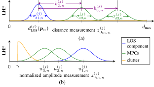
Figure 4: Visualization of (a) the joint distance LHF and (b) the joint amplitude LHF. The LOS distance is $d^{(j)}_{\text{LOS}}(\bm{p}_{n})=\lVert\bm{p}_{n}-\bm{p}_{\text{A}}^{(j)}\rVert$ and $\sigma_{\text{d}\hskip 0.5pt{k,n}}^{(j)}=\sigma_{\text{d}}(u^{(j)}_{k,n})$.

The LHF of the normalized amplitude measurement ${\mathsfbr{z}_{\mathrm{u}}^{(j)}}_{m,n}$ is obtained as

$$f({z_{\mathrm{u}}^{(j)}}_{m,n}|u^{(j)}_{k,n})\triangleq f_{\text{TRice}}\big{(}{z_{\mathrm{u}}^{(j)}}_{m,n};\sigma_{\mathrm{u}}(u^{(j)}_{k,n}),u^{(j)}_{k,n},\gamma\big{)}$$ (10)

with non-centrality parameter corresponding to the normalized amplitude $\mathsfbr{u}^{(j)}_{k,n}$ and $\gamma$ being the detection threshold of the CEDA. Again, the scale parameter is determined from the Fisher information given as $\sigma_{\mathrm{u}}^{2}(\mathsfbr{u}^{(j)}_{k,n})=1/2+\mathsfbr{u}^{(j)\hskip 0.5pt2}_{k,n}\,/(4N_{\text{s}})$ (see [32] for a detailed derivation). Note that this expression reduces to $1/2$ if the additive white Gaussian noise (AWGN) noise variance $\sigma^{(j)\hskip 0.5pt2}$ is assumed to be known or $N_{\text{s}}$ grows indefinitely. The probability of detection resulting from (10) is given by the Marcum Q-function, i.e., $p_{\text{d}}(\mathsfbr{u}_{k,n}^{(j)})\triangleq Q_{1}\big{(}{\mathsfbr{u}^{(j)}_{k,n}}/{\sigma_{\mathrm{u}}(\mathsfbr{u}^{(j)}_{k,n})},{\gamma}/{\sigma_{\mathrm{u}}(\mathsfbr{u}^{(j)}_{k,n})}\big{)}$ [43, 32].

False alarm measurements are assumed to be statistically independent of PBO states and are modeled by a Poisson point process with mean ${{\mu}_{\mathrm{fa}}}$ and PDF $f_{\mathrm{fa}}(\bm{z}_{m,n}^{(j)})$, which is assumed to factorize as $f_{\mathrm{fa}}(\bm{z}_{m,n}^{(j)})={f_{\mathrm{fa}}}({z_{\mathrm{d}}}_{m,n}^{(j)}){f_{\mathrm{fa}}}({z_{\mathrm{u}}}_{m,n}^{(j)})$. The clutter LHF of the distance measurement is uniformly distributed, i.e., ${f_{\mathrm{fa}}}({z_{\mathrm{d}}}_{m,n}^{(j)})=f_{\mathrm{U}}({z_{\mathrm{d}}}_{m,n}^{(j)},0,d_{\text{max}})$. The clutter LHF of the normalized amplitude is given by

$$f_{\mathrm{fa}}({z_{\mathrm{u}}^{(j)}}_{m,n})\triangleq f_{\text{TRayl}}({z_{\mathrm{u}}^{(j)}}_{m,n}\,;\sqrt{1/2}\,,\gamma)$$ (11)

with the scale parameter given as $\sqrt{1/2}$ and detection threshold $\gamma$. See Fig. 4 for a graphical representation of the joint likelihood function. We approximate the mean number of false alarms as $\mu_{\text{fa}}=N_{\text{s}}\,e^{-\gamma^{2}}$, where the right-hand side expression corresponds to the false alarm probability $p_{\text{fa}}(u)=\int f_{\text{TRayl}}(u\,;\sqrt{1/2}\,,\gamma)\,\mathrm{d}u=e^{-\gamma^{2}}$ according to (11).

IV-C State-Transition Model

For each PBO with state $\bm{\mathsfbr{y}}_{k,n-1}^{(j)}$ with $k\in\mathcal{K}_{n-1}^{(j)}$ at time $n-1$ and anchor $j$, there is one “legacy” PBO with state $\underline{\bm{\mathsfbr{y}}}_{k,n}^{(j)}\triangleq[\underline{\bm{\spsi}}_{k,n}^{(j)\hskip 0.5pt\mathrm{T}}\hskip 2.84526pt\underline{\mathsfbr{r}}_{k,n}^{(j)}]^{\mathrm{T}}$ with $k\in\mathcal{K}_{n-1}^{(j)}$ at time $n$ and anchor $j$. We also define the joint states $\underline{\bm{\mathsfbr{y}}}_{n}^{(j)}\!\triangleq[\underline{\bm{\mathsfbr{y}}}_{1,n}^{(j)\text{T}}\cdots\hskip 0.85358pt\underline{\bm{\mathsfbr{y}}}_{K_{n-1}^{(j)},n}^{(j)\text{T}}]^{\mathrm{T}}$ and $\underline{\bm{\mathsfbr{y}}}_{n}\!\triangleq[\underline{\bm{\mathsfbr{y}}}_{n}^{(1)\text{T}}\cdots\hskip 0.85358pt\underline{\bm{\mathsfbr{y}}}_{n}^{(J)\text{T}}]^{\mathrm{T}}$ as well as ${\bm{\mathsfbr{y}}}_{n}^{(j)}\!\triangleq[{\bm{\mathsfbr{y}}}_{1,n}^{(j)\text{T}}\cdots\hskip 0.85358pt{\bm{\mathsfbr{y}}}_{K_{n-1}^{(j)},n}^{(j)\text{T}}]^{\mathrm{T}}$ and ${\bm{\mathsfbr{y}}}_{n}\!\triangleq[{\bm{\mathsfbr{y}}}_{n}^{(1)\text{T}}\cdots\hskip 0.85358pt{\bm{\mathsfbr{y}}}_{n}^{(J)\text{T}}]^{\mathrm{T}}$. Assuming that the agent state as well as the PBO states evolve independently across $k$ and $n$ and $j$, the joint state-transition PDF factorizes as [30]

$$f(\bm{x}_{n},\underline{\bm{y}}_{n}|\bm{x}_{n-1},\bm{y}_{n-1})$$

$$\hskip 56.9055pt=f(\bm{x}_{n}|\bm{x}_{n-1})\prod_{j=1}^{J}\prod_{k=1}^{K_{n-1}^{(j)}}\!f(\underline{\bm{y}}_{k,n}^{(j)}|\bm{y}_{k,n-1}^{(j)})$$ (12)

where $f(\underline{\bm{y}}_{k,n}^{(j)}|\bm{y}_{k,n-1}^{(j)})=f(\underline{\bm{\psi}}_{k,n}^{(j)},\underline{r}_{k,n}^{(j)}|\bm{\psi}_{k,n-1}^{(j)},r_{k,n-1}^{(j)})$ is the augmented state-transition PDF. If a PBO did not exist at time $n-1$, i.e., $r_{k,n-1}^{(j)}=0$, it cannot exist at time $n$ as a legacy PBO. This means that

$$f(\underline{\bm{\psi}}_{k,n}^{(j)},\underline{r}_{k,n}^{(j)}|\bm{\psi}_{k,n-1}^{(j)},0)=\begin{cases}f_{\mathrm{d}}(\underline{\bm{\psi}}_{k,n}^{(j)}),&\underline{r}_{k,n}^{(j)}=0\\ 0,&\underline{r}_{k,n}^{(j)}=1\end{cases}\,.$$ (13)

If a PBO existed at time $n-1$, i.e., $r_{k,n-1}^{(j)}=1$, at time $n$ it either dies, i.e., $\underline{r}_{k,n}^{(j)}=0$, or it still exists, i.e., $\underline{r}_{k,n}^{(j)}=1$, with the survival probability denoted as $p_{\mathrm{s}}$. If it does survive, the PBO state $\underline{\bm{\spsi}}_{k,n}^{(j)}$ is distributed according to the state-transition PDF $f(\underline{\bm{\psi}}_{k,n}^{(j)}|\bm{\psi}_{k,n-1}^{(j)})$. Thus,

$$f(\underline{\bm{\psi}}_{k,n}^{(j)},\underline{r}_{k,n}^{(j)}|\bm{\psi}_{k,n\text{-}1}^{(j)},1)=\begin{cases}(1-p_{\mathrm{s}})f_{\mathrm{d}}(\underline{\bm{\psi}}_{k,n}^{(j)}),&\underline{r}_{k,n}^{(j)}=0\\ p_{\mathrm{s}}f(\underline{\bm{\psi}}_{k,n}^{(j)}|\bm{\psi}_{k,n\text{-}1}^{(j)}),&\underline{r}_{k,n}^{(j)}=1\end{cases}.$$ (14)

The agent state $\bm{\mathsfbr{x}}_{n}$ is assumed to evolve in time according to a 2-dimensional, constant-velocity and stochastic-acceleration model [44] (linear movement) given as $\bm{\mathsfbr{x}}_{n}=\bm{A}\,\bm{\mathsfbr{x}}_{n-1}+\bm{B}\,\bm{\mathsfbr{w}}_{n}$, with the acceleration process $\bm{\mathsfbr{w}}_{n}$ being i.i.d. across $n$, zero mean, Gaussian with covariance matrix ${\sigma_{\text{a}}^{2}}\,\bm{I}_{2}$; ${\sigma_{\text{a}}}$ is the acceleration standard deviation, and $\bm{A}\in\mathbb{R}^{\text{4x4}}$ and $\bm{B}\in\mathbb{R}^{\text{4x2}}$ are defined according to [44, p. 273], with observation period $\Delta T$. The PBO state-transition PDF is factorized as $f(\underline{\bm{\psi}}_{k,n}^{(j)}|\bm{\psi}_{k,n-1}^{(j)})=f(\underline{\bm{x}}_{\text{b}\hskip 0.5ptk,n}^{(j)}|\bm{x}_{\text{b}\hskip 0.5ptk,n-1}^{(j)})f(\underline{{u}}_{k,n}^{(j)}|{u}_{k,n-1}^{(j)})$. Similarly to the agent state, the legacy bias state $\underline{\bm{\mathsfbr{x}}}_{\text{b}\hskip 0.5ptk,n}^{(j)}$ is assumed to evolve in time linearly, according to a 1-dimensional, constant-velocity and stochastic-acceleration model $\underline{\bm{\mathsfbr{x}}}_{\text{b}\hskip 0.5ptk,n}^{(j)}=\bm{C}\,{\bm{\mathsfbr{x}}}_{\text{b}\hskip 0.5ptk,n-1}^{(j)}+\bm{D}\,\mathsfbr{w}_{\text{b}\hskip 0.5ptk,n}^{(j)}$, with the acceleration process $\mathsfbr{w}_{\text{b}\hskip 0.5ptk,n}^{(j)}$ being i.i.d. across $n$, $k$ and $j$, zero mean, Gaussian with standard deviation ${\sigma_{\text{b}}}$, and $\bm{C}\in\mathbb{R}^{\text{2x2}}$ and $\bm{D}\in\mathbb{R}^{\text{2x1}}$ also defined as in [44, p. 273]. The state-transition of the legacy normalized amplitude $\underline{\mathsfbr{u}}_{k,n}^{(j)}$, i.e., the state-transition PDF $f(\underline{u}_{k,n}^{(j)}|u_{k,n-1}^{(j)})$, is $\underline{\mathsfbr{u}}_{k,n}^{(j)}=\mathsfbr{u}_{k,n-1}^{(j)}+\mathsfbr{w}_{\text{u}\hskip 0.5ptk,n}^{(j)}$, where the noise $\mathsfbr{w}_{\text{u}\hskip 0.5ptk,n}^{(j)}$ is i.i.d. across $n$, $k$, and $j$, zero mean, Gaussian, with variance $\sigma^{2}_{\text{u}}$. Note that the temporal evolution of the distance biases $\mathsfbr{b}_{k,n}^{(j)}$ is generally non-linear, leading to a model mismatch. In most scenarios, however, it is well approximated as linear over short periods (see Sec. II).

IV-D New PBOs

Following [30, 14], newly detected PBOs at time $n$ and anchor $j$, i.e., PBOs that generate measurements for the first time at time $n$ and anchor $j$, are represented by new PBO states $\overline{\bm{\mathsfbr{y}}}_{m,n}^{(j)}\triangleq[\overline{\bm{\spsi}}_{m,n}^{(j)\hskip 0.5pt\mathrm{T}}\hskip 2.84526pt\overline{\mathsfbr{r}}_{m,n}^{(j)}]^{\mathrm{T}}$, $m\in\mathcal{M}_{n}^{(j)}$. New PBOs are modeled by a Poisson point process with mean number of new PBO ${\mu}_{\mathrm{n}}$ and PDF $f_{\mathrm{n}}(\overline{\bm{\psi}}_{m,n}^{(j)})$, where ${\mu}_{\mathrm{n}}$ is assumed to be a known constant. Each measurement $\bm{\mathsfbr{z}}_{m,n}^{(j)}$ gives rise to a new PBO $\overline{\bm{\mathsfbr{y}}}_{m,n}^{(j)}$. Thus, the number of new PBOs at time $n$ and anchor $j$ equals to the number of measurements $M_{n}^{(j)}$. Here, $\overline{r}_{m,n}^{(j)}=1$ means that the measurement $\bm{\mathsfbr{z}}_{m,n}^{(j)}$ was generated by a newly detected PBO. The state vector of all new PBOs at time $n$ and anchor $j$ is given by $\overline{\bm{\mathsfbr{y}}}_{n}^{(j)}\triangleq[\overline{\bm{\mathsfbr{y}}}_{1,n}^{(j)\hskip 0.5pt\mathrm{T}}\hskip 0.85358pt\cdots\hskip 0.85358pt\overline{\bm{\mathsfbr{y}}}_{\mathsfbr{M}_{n}^{(j)},n}^{(j)\hskip 0.5pt\mathrm{T}}]^{\mathrm{T}}$. The new PBOs become legacy PBOs at time $n+1$. Accordingly, the number of legacy PBOs is updated as $K_{n}^{(j)}=K_{n-1}^{(j)}+M_{n}^{(j)}$. The vector containing all PBO states at time $n$ is given by $\bm{\mathsfbr{y}}_{n}^{(j)}\triangleq[\underline{\bm{\mathsfbr{y}}}_{n}^{(j)\hskip 0.5pt\mathrm{T}}\hskip 2.84526pt\overline{\bm{\mathsfbr{y}}}_{n}^{(j)\hskip 0.5pt\mathrm{T}}]^{\mathrm{T}}$, with $\bm{\mathsfbr{y}}_{k,n}^{(j)}$ such that $k\in\mathcal{K}_{n}^{(j)}$. To avoid that the number of PBOs grows indefinitely, PBO states with low existence probability are removed as detailed in Section V.

IV-E Data Association Uncertainty

Estimation of multiple PBO states is complicated by the data association uncertainty, i.e., it is unknown which measurement $\bm{\mathsfbr{z}}_{m,n}^{(j)}$ originated from which PBO (see Fig. 2b). Furthermore, it is not known if a measurement did not originate from a PBO (false alarm), or if a PBO did not generate any measurement (missed detection). The associations between measurements and legacy PBOs are described by the PBO-oriented association vector $\underline{\bm{\mathsfbr{a}}}_{n}^{(j)}\triangleq[\underline{\mathsfbr{a}}_{1,n}^{(j)}\hskip 0.85358pt\cdots\hskip 0.85358pt\underline{\mathsfbr{a}}_{\mathsfbr{K}_{n-1},n}^{(j)}]^{\mathrm{T}}$ with entries $\underline{a}_{k,n}^{(j)}\triangleq m\in\mathcal{M}_{n}^{(j)}$, if legacy PBO $k$ generates measurement $m$, or $\underline{a}_{k,n}^{(j)}\triangleq 0$, if legacy PBO $k$ does not generate any measurement. In line with [52, 30, 14], the associations can be equivalently described by a measurement-oriented association vector $\overline{\bm{\mathsfbr{a}}}_{n}^{(j)}\triangleq[\overline{\mathsfbr{a}}_{1,n}^{(j)}\hskip 0.85358pt\cdots\hskip 0.85358pt\overline{\mathsfbr{a}}_{\mathsfbr{M}_{n},n}^{(j)}]^{\mathrm{T}}$ with entries $\overline{a}_{m,n}^{(j)}\triangleq k\in\mathcal{K}_{n-1}^{(j)}$, if measurement $m$ is generated by legacy PBO $k$, or $\overline{a}_{m,n}^{(j)}\triangleq 0$, if measurement $m$ is not generated by any legacy PBO. Furthermore, we assume that at any time $n$, each PBO can generate at most one measurement, and each measurement can be generated by at most one PBO (point target assumption) [52, 30, 14]. This is enforced by the exclusion functions $\Psi(\underline{\bm{a}}_{n}^{(j)},\overline{\bm{a}}_{n}^{(j)})$ and $\Gamma_{\underline{\bm{a}}_{n}^{(j)}}(\overline{r}_{m,n}^{(j)})$. The function $\Psi(\underline{\bm{a}}_{n}^{(j)},\overline{\bm{a}}_{n}^{(j)})=\prod_{k=1}^{K_{n-1}^{(j)}}\prod_{m=1}^{M_{n}^{(j)}}\psi(\underline{a}_{k,n}^{(j)},\overline{a}_{m,n}^{(j)})$ is defined as $\psi(\underline{a}_{k,n}^{(j)},\overline{a}_{m,n}^{(j)})=0$, if $\underline{a}_{k,n}^{(j)}=m$ and $\overline{a}_{m,n}^{(j)}\neq k$ or $\overline{a}_{m,n}^{(j)}=k$ and $\underline{a}_{k,n}^{(j)}\neq m$, otherwise it equals $1$. The function $\Gamma_{\underline{\bm{a}}_{n}^{(j)}}(\overline{r}_{m,n}^{(j)})=0$, if $\overline{r}_{m,n}^{(j)}=1$ and $\underline{a}_{k,n}^{(j)}=m$, otherwise it equals $1$. While $\Psi(\underline{\bm{a}}_{n}^{(j)},\overline{\bm{a}}_{n}^{(j)})$ enforces the point target assumption between individual legacy PBOs, $\Gamma_{\underline{\bm{a}}_{n}^{(j)}}(\overline{r}_{m,n}^{(j)})$ enforce it between each legacy PBO and the new PBOs. The “redundant formulation” of using $\underline{\bm{\mathsfbr{a}}}_{n}^{(j)}$ together with $\overline{\bm{\mathsfbr{a}}}_{n}^{(j)}$ is the key to making the algorithm scalable for large numbers of PBOs and measurements (see also the supplementary material [53, Sec. LABEL:M-sec:iterative_da]). The vectors containing all association variables for time $n$ are given by $\underline{\bm{\mathsfbr{a}}}_{n}\triangleq[\underline{\bm{\mathsfbr{a}}}_{1}^{(j)\hskip 0.5pt\mathrm{T}}\,...\,\underline{\bm{\mathsfbr{a}}}_{n}^{(j)\hskip 0.5pt\mathrm{T}}]^{\mathrm{T}}$, $\overline{\bm{\mathsfbr{a}}}_{n}\triangleq[\overline{\bm{\mathsfbr{a}}}_{1}^{(j)\hskip 0.5pt\mathrm{T}}\,...\,\overline{\bm{\mathsfbr{a}}}_{n}^{(j)\hskip 0.5pt\mathrm{T}}]^{\mathrm{T}}$.

A tabular summary of all random variables of the system model can be found in the supplementary material [53, Sec. LABEL:M-sec:system_model_table].

V Factor Graph and Sum-Product Algorithm

The problem considered is the sequential estimation of the agent state ${\bm{\mathsfbr{x}}}_{n}$ using all observed measurements $\bm{z}_{1:n}$ from all anchors up to time $n$. This is done in a Bayesian sense by calculating the minimum mean-square error (MMSE) [54] estimate of the extended agent state

$${\hat{{\bm{x}}}^{\text{MMSE}}_{n}\,\triangleq\int{\bm{x}}_{n}\,f({\bm{x}}_{n}|\bm{z}_{1:n})\,\mathrm{d}{\bm{x}}_{n}}$$ (15)

with $\hat{{\bm{x}}}^{\text{MMSE}}_{n}=[\hat{\bm{p}}^{\text{MMSE T}}_{n}$ $\hat{\bm{v}}^{\text{MMSE {T}}}_{n}]^{\text{T}}$ and $\bm{z}_{1:n}=[\bm{z}^{\text{T}}_{{1}}\,...\,\bm{z}^{\text{T}}_{n}]^{\text{T}}$. We also calculate the states of all detected PBOs

$$\hat{\bm{\psi}}^{(j)\hskip 0.5pt\text{MMSE}}_{k,n}\triangleq\int\bm{\psi}_{k,n}^{(j)}\,f(\bm{\psi}_{k,n}^{(j)}|r_{k,n}^{(j)}=1,\bm{z}_{1:n})\,\mathrm{d}\bm{\psi}_{k,n}^{(j)}$$ (16)

with $\hat{\bm{\psi}}_{k,n}^{(j)\hskip 0.5pt\text{MMSE}}=[\hat{b}_{k,n}^{(j)\hskip 0.5pt\text{MMSE}}\,\hat{v}_{\text{b}\hskip 0.5ptk,n}^{(j)\hskip 0.5pt\text{MMSE}}\,\hat{u}_{k,n}^{(j)\hskip 0.5pt\text{MMSE}}]^{\text{T}}$. A PBO is detected if $p(r_{k,n}^{(j)}=1|\bm{z}_{1:n})>p_{\mathrm{de}}$ [43], where $p_{\mathrm{de}}$ is the existence probability threshold not to be confused with $\lambda$, the detection threshold of the CEDA. The existence probabilities $p(r_{k,n}^{(j)}=1|\bm{z}_{1:n})$ are obtained from the marginal posterior PDFs of the PBO states, $f(\bm{y}_{k,n}^{(j)}|\bm{z}_{1:n})=f(\bm{\psi}_{k,n}^{(j)},r_{k,n}^{(j)}|\bm{z}_{1:n})$, according to

$$p({r}_{k,n}^{(j)}\!=\!1\big{|}\bm{z}_{1:n})=\int f({\bm{\psi}}_{k,n}^{(j)}\hskip 0.85358pt,r_{k,n}^{(j)}\!=\!1\big{|}\bm{z}_{1:n})\hskip 0.85358pt\mathrm{d}{\bm{\psi}}_{k,n}^{(j)}$$ (17)

and the marginal posterior PDFs $f(\bm{\psi}_{k,n}^{(j)}|r_{k,n}^{(j)}=1,\bm{z}_{1:n})$ are obtained from $f(\bm{\psi}_{k,n}^{(j)},r_{k,n}^{(j)}|\bm{z}_{1:n})$ as

$$f(\bm{\psi}_{k,n}^{(j)}|r_{k,n}^{(j)}=1,\bm{z}_{1:n})=\dfrac{f(\bm{\psi}_{k,n}^{(j)},r_{k,n}^{(j)}=1|\bm{z}_{1:n})}{p(r_{k,n}^{(j)}=1|\bm{z}_{1:n})}\hskip 0.85358pt.$$ (18)

We consider the estimates provided at time $n$ as “reliable” when the LOS component, i.e., the PBO at $k=1$, is detected by at least three anchors $j$, i.e., $|\mathcal{J}_{\text{LOS},n}|\geqslant 3$, where

$$\mathcal{J}_{\text{LOS},n}=\{\,j\in\{1,\hskip 0.5pt...\hskip 0.5pt,J\}\,|\,p(r_{1,n}^{(j)}=1|\bm{z}_{1:n})>p_{\mathrm{de}}\,\}\hskip 0.85358pt.$$ (19)

As the number of PBOs grows with time $n$ (at each time by $K_{n}^{(j)}=K_{n-1}^{(j)}+M_{n}^{(j)}$), PBOs with posterior existence probability $p(r_{k,n}^{(j)}=1|\bm{z}_{1:n})$ below a threshold $p_{\mathrm{pr}}$ are removed from the state space (“pruned”).

In order to obtain (15)-(18), the respective marginal posterior PDFs need to be calculated from the joint posterior PDF $f(\bm{x}_{0:n},\bm{y}_{1:n},\underline{\bm{a}}_{1:n},\overline{\bm{a}}_{1:n},\bm{m}_{1:n}|\bm{z}_{1:n})$ representing the statistical model discussed in Sec. IV. Since direct marginalization of the joint posterior PDF is computationally infeasible[30], we perform message passing by means of the SPA rules on the factor graph that represents the factorization of the joint posterior PDF.

V-A Joint Posterior and Factor Graph

The vectors containing all state variables for all times up to $n$ are given by $\bm{\mathsfbr{z}}_{1:n}=[\bm{\mathsfbr{z}}^{\text{T}}_{{1}}\,...\,\bm{\mathsfbr{z}}^{\text{T}}_{n}]^{\text{T}}$, ${\bm{\mathsfbr{x}}_{0:n}}=[{\bm{\mathsfbr{x}}}^{\text{T}}_{0}\,...\,{\bm{\mathsfbr{x}}}^{\text{T}}_{n}]^{\text{T}}$, $\underline{\bm{\mathsfbr{a}}}_{1:n}\triangleq[\underline{\bm{\mathsfbr{a}}}_{1}^{\text{T}}\,...\,\underline{\bm{\mathsfbr{a}}}_{n}^{\text{T}}]^{\text{T}}$, $\overline{\bm{\mathsfbr{a}}}_{1:n}\triangleq[\overline{\bm{\mathsfbr{a}}}_{1}^{\text{T}}\,...\,\overline{\bm{\mathsfbr{a}}}_{n}^{\text{T}}]^{\text{T}}$, $\bm{\mathsfbr{y}}_{1:n}=[\bm{\mathsfbr{y}}^{\text{T}}_{1}\,...\,\bm{\mathsfbr{y}}^{\text{T}}_{n}]^{\text{T}}$, and $\bm{\mathsfbr{m}}_{1:n}=[\bm{\mathsfbr{M}}^{\text{T}}_{1}\,...\,\bm{\mathsfbr{M}}^{\text{T}}_{n}]^{\text{T}}$. We now assume that the measurements $\bm{z}_{1:n}$ are observed and thus fixed. Applying Bayes’ rule as well as some commonly used independence assumptions[30, 14], the joint posterior PDF of all state variables $\bm{\mathsfbr{x}}_{0:n}$, $\bm{\mathsfbr{y}}_{1:n}$, $\underline{\bm{\mathsfbr{a}}}_{1:n}$, $\overline{\bm{\mathsfbr{a}}}_{1:n}$ ,$\bm{\mathsfbr{m}}_{1:n}$ up to time $n$ can be derived up to a constant factor as

$$f(\bm{x}_{0:n},\bm{y}_{1:n},\underline{\bm{a}}_{1:n},\overline{\bm{a}}_{1:n},\bm{m}_{1:n}|\bm{z}_{1:n})$$

$$\hskip 11.38109pt\propto f(\bm{x}_{0})\prod^{J}_{j^{\prime}=1}f(\underline{\bm{y}}^{(j^{\prime})}_{1,0})\prod^{n}_{n^{\prime}=1}\!\Phi_{\mathrm{x}}(\bm{x}_{n^{\prime}}|\bm{x}_{n^{\prime}-1})\prod^{J}_{j=1}\Psi\big{(}\underline{\bm{a}}^{(j)}_{n^{\prime}},\overline{\bm{a}}^{(j)}_{n^{\prime}}\big{)}$$

$$\hskip 11.38109pt\times\prod^{K^{(j)}_{n^{\prime}-1}}_{k=1}\Phi_{k}\big{(}\underline{\bm{y}}^{(j)}_{k,n^{\prime}}\big{|}\bm{y}^{(j)}_{k,n^{\prime}-1}\big{)}\underline{g}\big{(}\bm{x}_{n^{\prime}},\underline{\bm{\psi}}^{(j)}_{k,n^{\prime}},\underline{r}^{(j)}_{k,n^{\prime}},\underline{a}^{(j)}_{k,n^{\prime}};\bm{z}^{(j)}_{n^{\prime}}\big{)}$$

$$\hskip 11.38109pt\times\prod^{M^{(j)}_{n^{\prime}}}_{m=1}\overline{g}\big{(}\bm{x}_{n^{\prime}},\overline{\bm{\psi}}^{(j)}_{m,n^{\prime}},\overline{r}^{(j)}_{m,n^{\prime}},\overline{a}^{(j)}_{m,n^{\prime}};\bm{z}^{(j)}_{n^{\prime}}\big{)}$$ (20)

where we introduced the state-transition functions $\Phi_{\mathrm{x}}({\bm{x}}_{n}|{\bm{x}}_{n-1})\triangleq f({\bm{x}}_{n}|{\bm{x}}_{n-1})$, and $\Phi_{k}(\underline{\bm{y}}_{k,n}^{(j)}|\bm{y}_{k,n-1}^{(j)})\triangleq f(\underline{\bm{y}}_{k,n}^{(j)}|\bm{y}_{k,n-1}^{(j)})$, as well as the pseudo LHFs $\underline{g}\big{(}\bm{x}_{n},\underline{\bm{\psi}}^{(j)}_{k,n},\underline{r}^{(j)}_{k,n},\underline{a}^{(j)}_{k,n};\bm{z}^{(j)}_{n}\big{)}$ and $\overline{g}\big{(}\bm{x}_{n},\overline{\bm{\psi}}^{(j)}_{m,n},\overline{r}^{(j)}_{m,n},\overline{a}^{(j)}_{m,n};\bm{z}^{(j)}_{n}\big{)}$, for legacy PBOs and new PBOs, respectively.

For $\underline{g}\big{(}\bm{x}_{n},\underline{\bm{\psi}}^{(j)}_{k,n},\underline{r}^{(j)}_{k,n},\underline{a}^{(j)}_{k,n};\bm{z}^{(j)}_{n}\big{)}$ one obtains

$$\underline{g}\big{(}\bm{x}_{n},\underline{\bm{\psi}}^{(j)}_{k,n},1,\underline{a}^{(j)}_{k,n};\bm{z}^{(j)}_{n}\big{)}$$

$$\hskip 2.84526pt=\begin{cases}\displaystyle\frac{p_{\text{d}}({u}_{k,n}^{(j)})\hskip 0.85358ptf(\bm{z}_{m,n}^{(j)}|\bm{x}_{n},\underline{\bm{\psi}}_{k,n}^{(j)})}{\mu_{\mathrm{fa}}\hskip 0.85358ptf_{\mathrm{fa}}\big{(}\bm{z}^{(j)}_{m,n}\big{)}}\hskip 0.85358pt,&\underline{a}^{(j)}_{k,n}\!=m\in\!{\cal{M}}^{(j)}_{n}\\[12.80373pt] 1\!-p_{\text{d}}({u}_{k,n}^{(j)})\hskip 0.85358pt,&\underline{a}^{(j)}_{k,n}\!=0\end{cases}$$ (21)

and $\underline{g}\big{(}\bm{x}_{n},\underline{\bm{\psi}}^{(j)}_{k,n},0,\underline{a}^{(j)}_{k,n};\bm{z}^{(j)}_{n}\big{)}=1_{\{0\}}\big{(}\underline{a}^{(j)}_{k,n}\big{)}$. Similarly, for $\overline{g}\big{(}\bm{x}_{n},\overline{\bm{\psi}}^{(j)}_{m,n},\overline{r}^{(j)}_{m,n},\overline{a}^{(j)}_{m,n};\bm{z}^{(j)}_{n}\big{)}$ one can write

$$\overline{g}\big{(}\bm{x}_{n},\overline{\bm{\psi}}^{(j)}_{m,n},1,\overline{a}^{(j)}_{m,n};\bm{z}^{(j)}_{n}\big{)}$$

$$\triangleq\begin{cases}0\hskip 0.85358pt,&\overline{a}^{(j)}_{m,n}\!\in{\cal{K}}^{(j)}_{n-1}\\[4.2679pt] \displaystyle\frac{\mu_{\mathrm{n}}\hskip 0.85358ptf_{\mathrm{n}}(\overline{\bm{\psi}}_{m,n}^{(j)})\hskip 0.85358ptf(\bm{z}_{m,n}^{(j)}|\bm{x}_{n},\overline{\bm{\psi}}_{m,n}^{(j)})}{\mu_{\mathrm{fa}}\hskip 0.85358ptf_{\mathrm{fa}}\big{(}\bm{z}^{(j)}_{m,n}\big{)}}\hskip 0.85358pt,&\overline{a}^{(j)}_{m,n}=0\end{cases}$$ (22)

and $\overline{g}\big{(}\bm{x}_{n},\overline{\bm{\psi}}^{(j)}_{m,n},0,\overline{a}^{(j)}_{m,n};\bm{z}^{(j)}_{n}\big{)}\triangleq f_{\mathrm{d}}\big{(}\overline{\bm{\psi}}^{(j)}_{m,n}\big{)}$. The factor graph [40, 55] representing the factorization in (20) is shown in Fig. 5. Note that $\bm{\mathsfbr{m}}_{1:n}$ vanishes in (20) as it is fixed and thus constant, being implicitly defined by the measurements $\bm{z}_{1:n}$, and that the exclusion function $\Gamma_{\underline{\bm{a}}_{n}^{(j)}}(\overline{r}_{m,n}^{(j)})$ has been considered in (22). A detailed derivation of the joint posterior in (20) is given in [30, 14, 32].

V-B Marginal Posterior and Sum-Product Algorithm (SPA)

Since direct marginalization of the joint posterior PDF in (20) is infeasible, we use loopy message passing (belief propagation) [40] by means of the sum-product algorithm rules [40, 55] on the factor graph shown in Fig. 5. Due to the loops inside the factor graph, the resulting beliefs $q(\bm{x}_{n})$, ${q}(\underline{\bm{y}}_{k,n}^{(j)})={q}(\underline{\bm{\psi}}_{k,n}^{(j)},\underline{r}_{k,n}^{(j)})$, and ${q}(\overline{\bm{y}}_{m,n}^{(j)})={q}(\overline{\bm{\psi}}_{m,n}^{(j)},\overline{r}_{m,n}^{(j)})$ are only approximations of the respective posterior marginal PDFs. See the supplementary material [53, Sec. LABEL:M-sec:spa_messages] for a detailed derivation of the resulting SPA. Since the integrals involved in the calculations of the messages and beliefs cannot be obtained analytically, we use a computationally efficient sequential particle-based message passing implementation that performs approximate computations. As in [56], our implementation uses a “stacked state”, comprising the agent state as well as all PBO states. A detailed derivation of the particle-based implementation is also given in the supplementary material [53, Sec. LABEL:M-sec:particle_based_implementation].

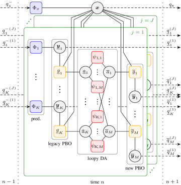
Figure 5: Factor graph corresponding to the factorization shown in (20). Dashed arrows represent messages that are only passed in one direction. The following short notations are used: $K\triangleq K_{n-1}^{(j)}$, $M\triangleq M_{n}^{(j)}$, $\underline{a}_{k}\triangleq\underline{a}_{k,n}^{(j)}$, $\overline{a}_{m}\triangleq\overline{a}_{m,n}^{(j)}$, $\bm{x}\triangleq\bm{x}_{n}$, $\underline{\bm{y}}_{k}\triangleq\underline{\bm{y}}_{k,n}^{(j)}$, $\overline{\bm{y}}_{m}\triangleq\overline{\bm{y}}_{m,n}^{(j)}$, $\Phi_{x}\triangleq\Phi_{x}(\bm{x}_{n}|\bm{x}_{n-1})$, $\Phi_{k}\triangleq\Phi_{k}(\underline{\bm{y}}_{k,n}^{(j)}|\bm{y}_{k,n-1}^{(j)})$, $\underline{g}_{k}\triangleq\underline{g}(\bm{x}_{n},$ $\underline{\bm{\psi}}^{(j)}_{k,n},\underline{r}^{(j)}_{k,n},\underline{a}^{(j)}_{k,n};\bm{z}^{(j)}_{n})$, $\overline{g}_{m}\triangleq\overline{g}(\bm{x}_{n},\overline{\bm{\psi}}^{(j)}_{m,n},\overline{r}^{(j)}_{m,n},\overline{a}^{(j)}_{m,n};\bm{z}^{(j)}_{n})$, $\psi_{k,m}\triangleq\psi(\underline{a}_{k,n}^{(j)},\overline{a}_{m,n}^{(j)})$, $q_{\mathrm{x}}\triangleq q(\bm{x}_{n})$, $\underline{q}_{k}^{(j)}\triangleq{q}(\underline{\bm{y}}_{k,n}^{(j)})$, $\overline{q}_{m}^{(j)}\triangleq{q}(\overline{\bm{y}}_{m,n}^{(j)})$, $q_{\mathrm{x}}^{-}\triangleq q(\bm{x}_{n-1})$, $\underline{q}_{k}^{-(j)}\triangleq{q}(\underline{\bm{y}}_{k,n-1}^{(j)})$.

The computational complexity scales only linearly in the number of particles $I$. The initial distributions $f(\bm{x}_{0})$ and $f(\underline{\bm{y}}^{(j)}_{1,0})$ are determined heuristically, using an initial measurement vector $\bm{z}_{0}$ containing $\bm{M}_{0}$ measurements. See [53, Sec. LABEL:M-sec:init_states] for details. For computational efficiency of the particle-based implementation, we approximate (10) by a truncated Gaussian PDF, i.e., we set $f({z_{\mathrm{u}}^{(j)}}_{m,n}|u^{(j)}_{k,n})\triangleq f_{\text{TN}}({z_{\mathrm{u}}^{(j)}}_{m,n};\sigma_{\mathrm{u}}(u^{(j)}_{k,n}),u^{(j)}_{k,n},\gamma)$.

VI Results

We validate the proposed algorithm by analyzing its performance using both synthetic data obtained using numerical simulation of different propagation scenarios and real radio measurements. The performance is compared with state-of-the-art multipath-aided positioning and tracking methods, including the MP-SLAM algorithm presented in [14, 15] and the multipath “cluster”-based robust positioning algorithm from [18]. For synthetic measurements, we also compare to the learning-based method introduced in [11], as well as to the hybrid approach from [28]. As a performance benchmark we provide the P-CRLB on the agent position error and compare to a particle-based variant of the multi-sensor AIPDA [36], which, in contrast to the other methods, does not facilitate multipath and, thus, acts as an additional baseline. Table I provides a summary of all reference methods along with their respective abbreviations. In the remainder of the paper, we use these abbreviations to refer to the respective methods. A detailed analysis of the runtime of all investigated methods can be found in the supplementary material [53, Sec. LABEL:M-sec:execution_time].

TABLE I: Reference methods and respective abbreviations

abbreviation	description
AIPDA	particle-based variant of the multi-sensor AIPDA [36]
MP-SLAM	multipath-based SLAM algorithm presented in [14, 15]
CLUSTER	multipath cluster-based robust tracking algorithm from [18]
ML-BIAS	learning-based bias mitigation algorithm presented in [11]
GP-TRACK	learning-based robust positioning method from [28]

VI-A Common Analysis Setup

The following setup and parameters are commonly used for all analyses presented unless noted otherwise.

To obtain the measurements $\bm{z}_{n,m}^{(j)}$ for each anchor $j$ at each time $n$ we used the CEDA from the supplementary material of [18]. The state transition variances are set as $\sigma_{a}=2~{}\mathrm{m/s^{2}}$, $\sigma_{\text{u}}=0.05\,\hat{u}_{n-1}^{(j)\hskip 0.5pt\text{MMSE}}$, $\sigma_{\text{b}}=0.05\,\hat{b}_{n-1}^{(j)\hskip 0.5pt\text{MMSE}}$. While $\sigma_{a}$ is set according to the maximum agent acceleration [57], for the state transition variances of all other parameters we use values proportional to the root mean squared error (RMSE) estimate of the previous time step $n-1$ as a heuristic. Note that this choice allows no tuning of the state transition variances to be required for all experiments presented, even though the propagation environments are considerably different. The particles for the initial state of a new PBO ${\overline{\bm{\spsi}}}_{m,n}^{(j)}$ are drawn from independent uniform distributions in the respective observation space, according to the joint PDF $f_{\mathrm{n}}\big{(}\overline{\bm{\psi}}_{m,n}^{(j)}\big{)}\triangleq f_{\mathrm{U}}(\overline{b}_{k,n}^{(j)};0,d_{\text{max}})\,f_{\mathrm{U}}(\overline{v}_{\text{b}\hskip 0.5ptk,n}^{(j)};-v_{\text{b}\hskip 0.5pt\text{max}},v_{\text{b}\hskip 0.5pt\text{max}})\,f_{\mathrm{U}}(\overline{u}_{k,n}^{(j)};0,u_{\text{max}})$, where the maximum normalized amplitude and bias velocity are assumed to be $u_{\text{max}}=40~{}\mathrm{dB}$ and $v_{\text{b}\hskip 0.5pt\text{max}}=4~{}\mathrm{m/s}$, respectively. The other simulation parameters are as follows: the survival probability is $p_{\mathrm{s}}=0.99$, the existence probability threshold is $p_{\mathrm{de}}=0.99$, the pruning threshold is $p_{\mathrm{pr}}=10^{-2}$, the mean number of newly detected MPCs is $\mu_{\mathrm{n}}=0.05$, the maximum number of message passing iterations for the loopy DA is $P=5000$ and the PDFs of the states are represented by $I=30^{4}$ particles each. We set the detection threshold to $\gamma=2$ ($6\,\mathrm{dB}$) for all simulations, which allows the algorithm to facilitate low-energy MPCs. For numerical stability, we reduced the root mean squared bandwidth $\beta_{\text{bw}}$ in (8) for MPCs (i.e., $k\in{2,\,...\,,K_{n}^{(j)}}$) by a factor of $1/3$. To prevent the algorithm after an OLOS situation from initializing a new PBO which competes with the explicit LOS component ($k=1$), we introduce a gate region according to [35, p. 95]. Measurements inside the gate region do not create new PBOs. The corresponding gate threshold is chosen such that the probability that the LOS measurement is inside the gate is 0.999.

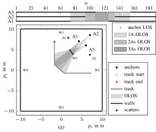
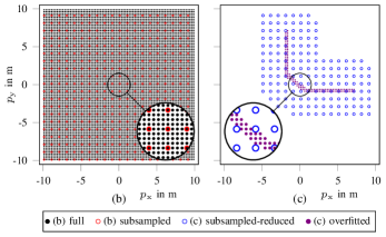
Figure 6: Graphical representation of the investigated synthetic experiments. Fig. (a) shows the simulated trajectory, anchor positions, walls, and OLOS intervals. Figs. (b) and (c) show the positions of all simulated training datasets.

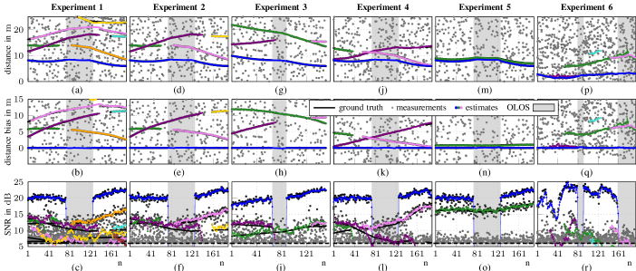
Figure 7: Single measurement realization in terms of distance, distance bias to the LOS component and SNR of anchor A1 for all six experiments investigated. We show the CEDA measurements together with the true values (for synthetic experiments) and the MMSE estimates of the proposed algorithm.

VI-A1 Implementation of Reference Methods

For consistency, the state-transition PDFs and initial state distributions of the agent state of all reference methods (and the normalized amplitude state of MP-SLAM, CLUSTER and AIPDA) are set as described in Sec. VI-A and [53, Sec. LABEL:M-sec:init_states]. All reference methods rely on particle-based state-space representations. In line with the proposed method, we used $30^{4}$ particles for MP-SLAM. As recommended in [28] and [18], we used $5000$ particles for state-space representation of all other reference methods. MP-SLAM is implemented according to [15, 14] using the measurements $\bm{z}_{m,n}^{(j)}$, i.e., distance and amplitude measurements, determined by applying the suggested CEDA to the individual radio signal vectors $\bm{r}_{n}^{(j)}$ as an input. The parameters of the dynamic object model (mean number of false alarms, mean number of potential VAs, probability of survival, pruning threshold) as well as detection threshold and the number of particles are set in accordance with Sec. VI-A. The anchor driving noise was set to $\sigma_{\text{An}}=0.02~{}\mathrm{m}$. In line with the proposed algorithm, we introduced a gate region as described in Sec. VI-A to prevent MP-SLAM from initializing new VAs after an OLOS situation, which compete with the physical anchors. For stability, we increased the distance measurement variances of all virtual anchors (not the physical anchors) by a factor of $3$ w.r.t. the Fisher information-based value. CLUSTER is implemented according to [18]. Again, we use the measurements $\bm{z}_{m,n}^{(j)}$ provided by the suggested CEDA as an input. AIPDA is implemented identically to CLUSTER assuming an uninformative NLOS distribution (conventional uniformly distributed clutter model[35]). Since ML-BIAS and GP-TRACK do not perform data association, we estimate the LOS component distance using a search-forward method[5]. On the interpolated Bartlett spectrum[58], we search in a super-resolution manner for the first maximum that exceeds a relative threshold, which we chose as six times the noise variance. The search-forward approach enables correctly identifying the LOS component (i.e., the first visible signal component), even when there are MPCs with amplitudes higher than that of the LOS component. GP-TRACK additionally applies to the received baseband signal vector $\bm{r}_{n}^{(j)}$ an autoencoder deep neural network (AE-DNN) compressing it into a small number of feature measurements, as well as a variational AE-DNN used for “anomaly detection”[25], i.e. data-driven identification of OLOS situations. Also a Gaussian process regression (GPR)-based LHF is learned for representing the fingerprint of NLOS measurements. We set up the AE-DNNs as well as the GPR using the configurations reported to yield the best performance in [28]. See the supplementary material [53, Sec. LABEL:M-sec:reference_methods_details] for details. GP-TRACK models the LOS component using a delay LHF with heuristically set variance values. To ensure a fair comparison, we instead use Fisher information-based variance values. For the ML-BIAS method, we provide results using the setup referred to as “GP”, which learns a bias correction term using GPR for the six parametric features suggested by the authors. After error correction according to [11] of the distance measurements (provided by the search-forward method), we applied a particle filter with Fisher information-based likelihood variances in line with the other compared methods.

VI-B Synthetic Radio Measurements (Experiments 1-5)

We evaluate the proposed algorithm using synthetic radio measurements, where the agent moves along a trajectory with two distinct direction changes as shown in Fig. 6. The agent is observed at $N=190$ discrete time steps $n\in\{1,\,...\,,N\}$ at a constant observation rate of $\Delta T=100\,\mathrm{ms}$, resulting in a continuous observation time of $19\,\mathrm{s}$. We simulate three anchors, labeled A1-A3 in Fig. 6, which are placed in close vicinity to each other. The limited directional diversity of the anchors (corresponding to a poor geometric dilution of precision (GDOP) [59]) poses a challenging setup for delay-measurement-based position estimation. We choose the transmitted signal to be of root-raised-cosine shape with a roll-off factor of $0.6$ and a $3$-dB bandwidth of $500\,\mathrm{MHz}$. The received baseband signal is critically sampled, i.e., $T_{\text{s}}=1.25\,\mathrm{ns}$, with a total number of $N_{\text{s}}=81$ samples, amounting to a maximum distance $d_{\text{max}}=30\,\mathrm{m}$. The normalized amplitudes (SNRs) of the LOS component as well as the MPCs are set to $38~{}\mathrm{dB}$ at an LOS distance of $1~{}\mathrm{m}$. Unless otherwise noted, the normalized amplitudes of the individual MPCs are assumed to follow free-space path loss and are additionally attenuated by $3~{}\mathrm{dB}$ per reflection (e.g. $6~{}\mathrm{dB}$ for double-bounce reflections). We show results of 5 synthetic experiments, referred to as Experiment 1-5. The environment setup (i.e., walls and scatters) differs for the individual experiments as detailed in the following. For all experiments investigated, the anchors are obstructed by an obstacle, labeled W5 in Fig. 6, which leads to partial and full OLOS situations in the center of the track.

Figs. 7a-o provide a graphical representation of the observation space of anchor A1 for all experiments. It shows the measurements obtained by the CEDA in distance, distance bias and SNR domain together with the ground truth values, and the respective MMSE estimates of the proposed algorithm. The distance bias is obtained by subtracting the LOS distance for the true agent position from the respective PBO distances values. For Fig. 7, we used $p_{\mathrm{de}}=0.011$ to visualize all PBOs available.

Training of Reference Methods

Training of the method from [28] involves a two step procedure. In the first training step, both AE-DNNs are trained using $6400$ unlabeled samples of baseband signal vectors that cover the entire floorplan, constituting a two dimensional grid from $-10$ m to $10$ m in $p_{\text{x}}$ and $p_{\text{y}}$ directions with $0.25$ m spacing. The AE-DNN used for “anomaly detection” additionally requires LOS-only data (i.e., no OLOS situations). Thus, we created two training datasets, once deactivating the obstacle (W5). In the second training step GPR is used to learn a feature-based measurement model using samples of baseband signal vectors (preprocessed by the feature extraction AE-DNNs) labeled with their respective positions. We use a similar grid that also covers the entire floorplan, but with $1$ m grid spacing. The respective positions of both training datasets are depicted in Fig. 6b. Training of the method from [11] requires only one set of baseband signal data labeled with their respective positions. Here, we instead provide results using the two different training datasets depicted in Fig. 6c. The “reduced” dataset consists of positions where the overall received signal power remains within a moderate range. We found a low received signal to be detrimental for this method leading to strong fluctuations of the distance error for adjacent positions. Additionally, we used an “overfitted” dataset, which contains only data located around the trajectory. In line with the proposed method, the AIPDA, the MP-SLAM, and the CLUSTER algorithms require no training.

Experiment 1 – High Information

In this experiment, the ground truth MPC positions and corresponding distances are calculated based on the VA model (single-bounce and double-bounce reflections only), assuming the walls to act as large, flat surfaces. We use all walls (W1 to W4) of the floor plan shown in Fig. 6. Note that the image sources (VAs) caused by walls W1-W4 are also obstructed by the obstacle (W5). This experiment represents a “high information” environment as several high-SNR MPCs are caused by walls arranged convexly all around the trajectory.

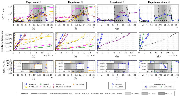
Figure 8: Performance in terms of the RMSE of the estimated agent position over time $n$ in (a),(d),(g),(j), in terms of the cumulative frequency of the estimated agent position error in inverse logarithmic scale in (b),(e),(h),(k) , and the relative number of reliable estimates per time $n$ in (c),(f),(i),(l) for Experiment 1 in (a)-(c), for Experiment 2 in (d)-(f), for Experiment 3 in (g)-(i), and for Experiment 4 and 5 in (j)-(l). Note that legends vary between the experiments. The performance baselines (see Sec. VI-D1) for Experiment 4 and 5 are identical. Thus, the results are presented in a single plot for the sake of brevity.

Experiment 2 – Low Information

In line with Experiment 1, the ground truth MPC positions and corresponding distances in this experiment are calculated based on the VA model. However, for this experiment we only use walls W1 to W2 of the floor plan shown in Fig. 6 (single-bounce reflections only). This experiment represents a “low-information” environment with few MPCs that are caused by walls whose VAs take similar directions w.r.t. the agent as the physical anchors. This leads to all image sources (created by W1 and W2) being temporarily obstructed by the obstacle W5 as the agent moves along the trajectory (see Figs. 7d-f).

Experiment 3 – Appearing Obstruction

In line with Experiment 2, the ground truth MPC positions and corresponding distances are calculated based on the VA model using only walls W1 and W2 of the floor plan shown in Fig. 6. However, we assume the obstacle (W5) to appear at time $n=67$. Additionally, we have shifted wall W1 by three meters in y direction, i.e., it reaches from $[-10~{}13]$ to $[10~{}13]$. This leads to several image sources (VAs) of all anchors disappearing simultaneously with the LOS component, i.e., the MPC visibility changes when the OLOS situation occurs (see Figs. 7g-i). Note that for this experiment, we shortened the trajectory, covering only the second turn during full OLOS.

Experiment 4 – Scatter

In this experiment, the ground truth MPC positions and corresponding distances are calculated based on the the scatters S1 and S2 of the floor plan shown in Fig. 6, which are the only source of multipath propagation. The MPC distances are calculated as the sum of the respective scatter-anchor distances and the scatter-agent distances. The ground truth amplitudes are obtained assuming free-space path loss for both, the scatter-anchor distance and the scatter-agent distance [12], and lossless re-scattering. In this experiment, the resulting MPCs interfere strongly with the LOS component (see Figs. 7j-l), when a scatter is near the path between agent and anchor. Thus, to obtain measurements $\bm{z}_{n,m}^{(j)}$, we used the CEDA from [50] with adaptive initialization for new components[49], which provides increased reliability considering the correlations between individual signal components (at the cost of increased computational complexity).

Experiment 5 – Ground Reflection

In this experiment, the ground truth MPC positions and corresponding distances are again calculated from the VA model. However, we assume multipath propagation to be caused by ground reflection assuming the agent as well as all anchors to be at a height of $1$ m w.r.t. the ground. For demonstration, we assume that the corresponding VAs are not obstructed by the obstacle (W5).

VI-C Real Radio Measurements (Experiment 6)

In this experiment, we use real radio measurements collected in a laboratory hall of NXP Semiconductors, Gratkorn, Austria. The hall features a wide, open space and includes a demonstration car (Lancia Thema 2011), furniture, and metallic surfaces, thereby representing a typical multipath-prone industrial environment. An agent is assumed to move along a pseudo-random trajectory (selected out of a grid of agent positions), obtained in a static measurement setup. We selected $N=195$ measurements, assuming a sampling rate of $\Delta T=170\,\mathrm{ms}$. The agent velocity is set to vary around a magnitude of $0.35\,\mathrm{m/s}$. This leads to a corresponding continuous observation time $33.15\,\mathrm{s}$. At each selected position, a radio signal was transmitted from the assumed agent position, which was received by 4 anchors. The agent was represented by a polystyrene build, while the anchor antennas were mounted on the demonstration car. The agent as well as the anchors were equipped with a dipole antenna with an approximately uniform radiation pattern in the azimuth plane and zeros in the floor and ceiling directions. The radio signal was recorded by an M-sequence correlative channel sounder with frequency range $3-10\,\mathrm{GHz}$. Within the measured band, the actual signal band was selected by a filter with raised-cosine impulse response $s(t)$, with a roll-off factor of $0.6$, a two-sided 3-dB bandwidth of $499.2\,\mathrm{MHz}$ and a center frequency of $7.9872\,\mathrm{GHz}$, corresponding to channel 9 of IEEE 802.15.4a. We used $N_{\text{s}}=81$ samples, amounting to a $d_{\text{max}}$ slightly below $30\,\mathrm{m}$. We created two full OLOS situations at $n\in[80,92]$ and $n\in[159,170]$ using an obstacle consisting of a metal plate covered with attenuators. A floor plan showing the track, the environment (i.e, the car, other reflecting objects and walls), the antenna positions, and the OLOS conditions w.r.t. all antennas is given in Fig. 9. Pictures of the measurement setup are provided in the supplementary meterial [53, Sec. LABEL:M-sec:measurement_photos_nxp]. The metal surface of the car strongly reflected the radio signal, leading to a radiation pattern of $270^{\circ}$ for A1 and A2 and $180^{\circ}$ for A3 and A4. Thus, during large parts of the trajectory, the LOS of 2 or 3 out of 4 anchors was not available. Moreover, the pulse reflected by the car surface strongly interfered with the LOS pulse, leading to significant fluctuations of the amplitudes. Also, this leads to the channel estimator being prone to produce a high-SNR component just after the LOS component.

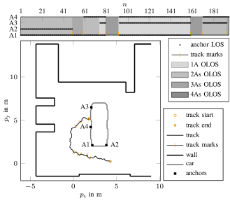
Figure 9: Measurement setup for Experiment 6 using real radio-signals.

As only two antennas (A1 and A2) are visible at the track starting point, the position estimate obtained by trilateration is ambiguous. In the scenario presented, the relative antenna position w.r.t. the car can be assumed to be known. Thus, for this experiment, we used the antenna pattern as prior information for initialization of the position state. For the numerical evaluation presented, we added AWGN to the real radio signal obtained. We set $\lVert\bar{\bm{r}}_{\mathrm{raw}}^{(j)}\rVert^{2}/\sigma^{(j)\hskip 0.5pt2}=20\text{dB}$, where $\lVert\bar{\bm{r}}_{\mathrm{raw}}^{(j)}\rVert^{2}$ is the average energy of the real measured signal per anchor $j$. Figs. 7q-r show the observation space of anchor A1 for this experiment.

VI-D Joint Performance Evaluation

We provide the performance of the proposed algorithm and all applicable reference methods for all investigated experiments in Figs. 8, and 10.

VI-D1 Performance Metrics and Baseline

For each of the experiments investigated, we analyze the performance in terms of both, the RMSE of the estimated agent position over time $n$ given as $e_{n}^{\text{RMSE}}~{}=~{}\sqrt{\mathbb{E}\left\{\lVert\hat{\bm{p}}^{\text{MMSE}}_{n}-\bm{p}_{n}\rVert^{2}\right\}}$ and the cumulative frequency of the magnitude error of the estimated agent position $e_{n}\triangleq\lVert\hat{\bm{p}}^{\text{MMSE}}_{n}-\bm{p}_{n}\rVert$, and are evaluated using a numerical simulation with 500 realizations. As a performance benchmark, we provide the Cramér-Rao lower bound (CRLB) on the position error variance considering all visible LOS measurements of a single time step $n$, which we refer to as the snapshot-based positioning CRLB (SP-CRLB) [60, 8]. Furthermore, we provide the corresponding posterior Cramér-Rao lower bound (P-CRLB) [41] that additionally considers the dynamic model of the agent state, and the “P-CRLB-LOS” that corresponds to the P-CRLB assuming the LOS component to all anchors is always available and, thus, provides a lower bound for the proposed estimator. See the supplementary material of [18, Sec. VI] for a detailed derivation.

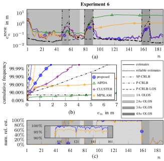
Figure 10: Performance for Experiment 6 in terms of the RMSE of the estimated agent position over time $n$ in (a), the cumulative frequency of the agent position error in inverse logarithmic scale in (b) , and the relative number of reliable estimates per time $n$ in (c).

VI-D2 Overall performance

Figs. 8, and 10 show in solid lines (termed “all estimates”) the performance considering the estimates of every realization of the performed numerical simulations of at all times $n\in\{1,\,...\,,N\}$ (c.f. Sec. VI-D3). Analyzing the performance of the proposed method across all experiments, it can not only utilize the position information contained in MPCs caused by flat surfaces (VA model), as shown in Experiment 1, 2, and 3, but it can also leverage MPCs caused by scatters, as demonstrated in Experiment 4, and three dimensional structures, such as the ground reflections in Experiment 5 (that lead to distance biases that evolve approximately linear over time $n$). Its RMSE attains the P-CRLB in LOS conditions and outperforms it during full OLOS situations due to the additional information provided by the MPCs. However, we observe a slightly reduced performance for Experiment 4, which is due to the small distance between LOS and MPCs w.r.t. the bandwidth of the simulated UWB system, in particular during initialization (see Fig. 7j). While CLUSTER also manages to maintain the track in every single realization, it shows reduced performance in Experiment 1, 2, and 6 during the OLOS situation, which is due to the approximate nature and resulting reduced curvature of its measurement model. Furthermore, in Experiment 3 the method diverged in about $50\%$ of the simulation runs. This is due to the simultaneous disappearance of the LOS component (i.e, the start of the OLOS situation) and the first MPC as illustrated in Fig. 7g, which significantly alters the shape of the observed “multipath cluster” and, thus, violates the system model of this method. MP-SLAM can achieve a significantly reduced RMSE in high-information scenarios with many reflecting surfaces. This is shown in Experiment 1, where MP-SLAM clearly outperforms the proposed algorithm in terms of accuracy (see e.g. Fig. 8b). Examining Fig. 8a, we even observe the RMSE of the MP-SLAM method to fall below the P-CRLB in the first part of the OLOS situation. This is possible due to the additional position information provided by the MPCs measurements (associated to the jointly inferred VAs) as investigated in [61, 2]. However, as visible in Figs. 8a and b, in 6 realizations MP-SLAM loses the track after the full OLOS situation, while the proposed algorithm keeps the track for every realization. A possible explanation is the reduced number of dimensions of the PBO model (1-D distance bias) w.r.t. MP-SLAM (2-D VA position) and the associated reduced chance of all particles converging to a wrong mode. In the low-information scenario investigated in Experiment 2, MP-SLAM diverges in about $50\%$ of the simulation runs. This is due to the geometric ambiguity of the scenario leading to the estimated agent distribution collapsing to an ambiguous mode. The AIPDA method does not facilitate multipath at all, acting as a baseline that emphasizes the challenging nature of the investigated experiments. While it shows excellent performance in LOS conditions, it follows ambiguous paths (i.e., it loses the track) after the full OLOS situation for many realizations, leading to a significantly reduced performance. While GP-TRACK significantly outperforms the AIPDA method, which demonstrates the effectiveness of the learned multipath representation, it shows reduced overall accuracy by not attaining the P-CRLB in LOS conditions, as well as reduced robustness by losing the track in many realizations. The reduced accuracy of GP-TRACK is caused by the insufficient precision of the learned geometric imprint that interferes with the LOS model. Possible explanations for the reduced robustness are both, the significant number of false alarms of the anomaly detection method and the reduced robustness of the conventional particle filter w.r.t. PDA-type filters [35] (see also the supplementary material [53, Sec. LABEL:M-sec:message_interpretation]). Finally, the ML-BIAS method performs robustly, not showing any lost tracks when using the “overfitted” training dataset, which confirms the validity of our implementation. Yet, it still shows a low overall accuracy not attaining the P-CRLB in LOS condition. In contrast, for the “subsampled-reduced” dataset, the method failed to produce consistent estimates, leading to divergence of the subsequently applied particle filter. This is due to the fact, that the bias representations are learned per anchor, i.e., the features that lead to the bias estimate cannot offer angular information. Furthermore, jumps in the estimated delay can lead to instability of the method as we can only apply the particle filter to the corrected estimate, which is in contrast to the “soft” information fusion offered by PDA-type methods including the proposed algorithm.

The results using real radio measurements in Experiment 6 confirm the validity of the numerical results presented. We observe a consistent performance gain of the proposed algorithm w.r.t. the reference methods. However, different to Experiment 1 to 5, in Experiment 6 all presented algorithms fail to reach the P-CRLB over parts of the track, as can be observed from Fig. 10. The exact consistency in progression of the RMSE curves suggests unmodeled effects (e.g. diffraction at the vehicle body) as well as inaccuracies in the reference as a probable reason.

VI-D3 Identification of Unreliable Measurements

For the proposed algorithm and the MP-SLAM method, Figs. 8 and 10 show results considering estimates identified as reliable according to (19), termed “reliable estimates only” (dotted lines). Additionally, Figs. 8 and 10 show the relative number of reliable estimates over time $n$. Analyzing the performance of both methods across all experiments investigated, they consistently identify outliers and, thus, they almost attain the P-CRLB-LOS. The MP-SLAM method falls even slightly below the P-CRLB-LOS in Experiment 1 and 2, due to the additional information provided by the MPCs. However, while the number of reliable measurements for MP-SLAM is reduced after the full OLOS situation, especially for Experiment 2, the proposed method provides $100\%$ reliable estimates with all runs converging after the full OLOS situation. Consistent with the observations from Sec. VI-D2, we notice a slightly reduced number of reliable estimates of the proposed method for Experiment 4. However, it still identifies unreliable estimates, only slightly exceeding the P-CRLB-LOS.

VII Conclusion

We presented a particle-based SPA that sequentially estimates the position of a mobile agent using range and amplitude measurements provided by a snapshot-based channel estimation and detection algorithm (CEDA). We analyzed the performance of the proposed algorithm using numerically simulated radio signals and real radio measurements in different propagation environments, comprising flat surfaces (e.g., walls and floor) and scatters. We showed that the additional information provided by the PBOs can support the estimation of the agent position. Furthermore, we demonstrated the capability of the proposed method to identify unreliable measurements and, thus, to identify lost tracks. Our algorithm outperforms state-of-the-art methods for MPC-aided robust positioning and tracking and consistently attains the P-CRLB in partial obstructed line-of-sight (OLOS) situations. While multipath-based SLAM (MP-SLAM) can naturally provide high-accuracy results in environments with flat surfaces that offer high geometric diversity, we have shown that the proposed method consistently provides a lower number of lost tracks.

Possible directions for future research include extending the model to diffuse MPC that lead to multiple measurements by using data association with extended objects [31].

References

- [1] K. Witrisal, P. Meissner et al., “High-accuracy localization for assisted living: 5G systems will turn multipath channels from foe to friend,” IEEE Signal Process. Mag., vol. 33, no. 2, pp. 59–70, Mar. 2016.
- [2] R. Mendrzik, H. Wymeersch, G. Bauch, and Z. Abu-Shaban, “Harnessing NLOS components for position and orientation estimation in 5G Millimeter Wave MIMO,” IEEE Trans. Wireless Commun., vol. 18, no. 1, pp. 93–107, 2019.
- [3] R. Karlsson and F. Gustafsson, “The future of automotive localization algorithms: Available, reliable, and scalable localization: Anywhere and anytime,” IEEE Signal Process. Mag., vol. 34, no. 2, pp. 60–69, 2017.
- [4] J. Ko, T. Gao, R. Rothman, and A. Terzis, “Wireless sensing systems in clinical environments: Improving the efficiency of the patient monitoring process,” IEEE Eng. Med. Biol. Mag., vol. 29, pp. 103–9, 05 2010.
- [5] D. Dardari, A. Conti, U. Ferner, A. Giorgetti, and M. Z. Win, “Ranging with ultrawide bandwidth signals in multipath environments,” Proc. IEEE, vol. 97, no. 2, pp. 404–426, Feb. 2009.
- [6] L. Taponecco, A. D’Amico, and U. Mengali, “Joint TOA and AOA estimation for UWB localization applications,” IEEE Trans. Wireless Commun., vol. 10, no. 7, pp. 2207–2217, 2011.
- [7] F. Rusek, D. Persson, B. K. Lau, E. G. Larsson, T. L. Marzetta, O. Edfors, and F. Tufvesson, “Scaling up MIMO: Opportunities and challenges with very large arrays,” IEEE Signal Process. Mag., vol. 30, no. 1, pp. 40–60, Jan. 2013.
- [8] Y. Shen and M. Z. Win, “Fundamental limits of wideband localizationpart I: A general framework,” IEEE Trans. Inf. Theory, vol. 56, no. 10, pp. 4956–4980, 2010.
- [9] S. Aditya, A. F. Molisch, and H. M. Behairy, “A survey on the impact of multipath on wideband time-of-arrival based localization,” Proc. IEEE, vol. 106, no. 7, pp. 1183–1203, 2018.
- [10] W. M. Gifford, D. Dardari, and M. Z. Win, “The impact of multipath information on time-of-arrival estimation,” IEEE Trans. Signal Process., vol. 70, pp. 31–46, 2022.
- [11] H. Wymeersch, S. Maranò, W. M. Gifford, and M. Z. Win, “A machine learning approach to ranging error mitigation for UWB localization,” IEEE Trans. Wireless Commun., vol. 60, no. 6, pp. 1719–1728, 2012.
- [12] C. Gentner, T. Jost, W. Wang, S. Zhang, A. Dammann, and U. C. Fiebig, “Multipath assisted positioning with simultaneous localization and mapping,” IEEE Trans. Wireless Commun., vol. 15, no. 9, pp. 6104–6117, Sep. 2016.
- [13] A. Shahmansoori, G. E. Garcia, G. Destino, G. Seco-Granados, and H. Wymeersch, “Position and orientation estimation through mm Wave MIMO in 5G systems,” IEEE Trans. Wireless Commun., vol. 17, no. 3, pp. 1822–1835, Mar. 2018.
- [14] E. Leitinger, F. Meyer, F. Hlawatsch, K. Witrisal, F. Tufvesson, and M. Z. Win, “A belief propagation algorithm for multipath-based SLAM,” IEEE Trans. Wireless Commun., vol. 18, no. 12, pp. 5613–5629, 2019.
- [15] E. Leitinger, S. Grebien, and K. Witrisal, “Multipath-based SLAM exploiting AoA and amplitude information,” in Proc. IEEE ICCW-19, Shanghai, China, May 2019, pp. 1–7.
- [16] H. Kim, K. Granström, L. Gao, G. Battistelli, S. Kim, and H. Wymeersch, “5G mmWave cooperative positioning and mapping using multi-model PHD filter and map fusion,” IEEE Trans. Wireless Commun., vol. 19, no. 6, pp. 3782–3795, Mar. 2020.
- [17] T. Pedersen, “Modeling of path arrival rate for in-room radio channels with directive antennas,” IEEE Trans. Antennas Propag., vol. 66, no. 9, pp. 4791–4805, 2018.
- [18] A. Venus, E. Leitinger, S. Tertinek, and K. Witrisal, “A graph-based algorithm for robust sequential localization exploiting multipath for obstructed-LOS-bias mitigation,” IEEE Trans. Wireless Commun., 2023.
- [19] L. Wielandner, A. Venus, T. Wilding, and E. Leitinger, “Multipath-based SLAM for non-ideal reflective surfaces exploiting multiple-measurement data association,” ArXiv e-prints, 2023. [Online]. Available: http://arxiv.org/abs/2304.05680
- [20] Z. Yu, Z. Liu, F. Meyer, A. Conti, and M. Z. Win, “Localization based on channel impulse response estimates,” in Proc. IEEE/ION PLANS-20, 2020, pp. 1014–1021.
- [21] H. Kim, K. Granstrom, L. Svensson, S. Kim, and H. Wymeersch, “PMBM-based SLAM filters in 5G mmWave vehicular networks,” IEEE Trans. Veh. Technol., pp. 1–1, May 2022.
- [22] M. Krekovic, I. Dokmanic, and M. Vetterli, “Shapes from echoes: Uniqueness from point-to-plane distance matrices,” IEEE Trans. Signal Process., vol. 68, pp. 2480–2498, 2020.
- [23] S. Marano and, W. Gifford, H. Wymeersch, and M. Win, “NLOS identification and mitigation for localization based on UWB experimental data,” IEEE J. Sel. Areas Commun., vol. 28, no. 7, pp. 1026 –1035, Sept. 2010.
- [24] Y. Li, S. Mazuelas, and Y. Shen, “A semi-supervised learning approach for ranging error mitigation based on UWB waveform,” in Proc. IEEE MILCOM-21, 2021, pp. 533–537.
- [25] M. Stahlke, S. Kram, F. Ott, T. Feigl, and C. Mutschler, “Estimating TOA reliability with variational autoencoders,” IEEE Sensors J., pp. 1–1, 2021.
- [26] Y. Huang, S. Mazuelas, F. Ge, and Y. Shen, “Indoor localization system with NLOS mitigation based on self-training,” IEEE Trans. Mobile Comput., pp. 1–1, 2022.
- [27] A. Conti, S. Mazuelas, S. Bartoletti, W. C. Lindsey, and M. Z. Win, “Soft information for localization-of-things,” Proc. IEEE, vol. 107, no. 11, pp. 2240–2264, Nov. 2019.
- [28] S. Kram, C. Kraus, T. Feigl, M. Stahlke, J. Robert, and C. Mutschler, “Position tracking using likelihood modeling of channel features with Gaussian processes,” ArXiv e-prints, vol. abs/2203.13110, 2022. [Online]. Available: http://arxiv.org/abs/2203.13110
- [29] Y. Bar-Shalom, F. Daum, and J. Huang, “The probabilistic data association filter,” IEEE Control Syst. Mag., vol. 29, no. 6, pp. 82–100, Dec 2009.
- [30] F. Meyer, T. Kropfreiter, J. L. Williams, R. Lau, F. Hlawatsch, P. Braca, and M. Z. Win, “Message passing algorithms for scalable multitarget tracking,” Proc. IEEE, vol. 106, no. 2, pp. 221–259, Feb. 2018.
- [31] F. Meyer and J. L. Williams, “Scalable detection and tracking of geometric extended objects,” IEEE Trans. Signal Process., vol. 69, pp. 6283–6298, Oct. 2021.
- [32] X. Li, E. Leitinger, A. Venus, and F. Tufvesson, “Sequential detection and estimation of multipath channel parameters using belief propagation,” IEEE Trans. Wireless Commun., vol. 21, no. 10, pp. 8385–8402, Apr. 2022.
- [33] M. S. Arulampalam, S. Maskell, N. Gordon, and T. Clapp, “A tutorial on particle filters for online nonlinear/non-Gaussian Bayesian tracking,” IEEE Trans. Signal Process., vol. 50, no. 2, pp. 174–188, Feb. 2002.
- [34] H. Durrant-Whyte and T. Bailey, “Simultaneous localization and mapping: Part I,” IEEE Robot. Autom. Mag., vol. 13, no. 2, pp. 99–110, Jun. 2006.
- [35] Y. Bar-Shalom and X.-R. Li, Multitarget-Multisensor Tracking: Principles and Techniques. Storrs, CT, USA: Yaakov Bar-Shalom, 1995.
- [36] S. Jeong and J. Tugnait, “Multisensor tracking of a maneuvering target in clutter using IMMPDA filtering with simultaneous measurement update,” IEEE Trans. Aerosp. Electron. Syst., vol. 41, no. 3, pp. 1122–1131, Nov. 2005.
- [37] D. Lerro and Y. Bar-Shalom, “Automated tracking with target amplitude information,” in 1990 American Control Conference, May 1990, pp. 2875–2880.
- [38] S. Zhang, E. Staudinger, T. Jost, W. Wang, C. Gentner, A. Dammann, H. Wymeersch, and P. A. Hoeher, “Distributed direct localization suitable for dense networks,” IEEE Trans. Aerosp. Electron. Syst., vol. 56, no. 2, pp. 1209–1227, July 2020.
- [39] T. Kropfreiter, J. L. Williams, and F. Meyer, “A scalable track-before-detect method with Poisson/multi-Bernoulli model,” in Proc. IEEE FUSION-21, 2021.
- [40] F. Kschischang, B. Frey, and H.-A. Loeliger, “Factor graphs and the sum-product algorithm,” IEEE Trans. Inf. Theory, vol. 47, no. 2, pp. 498–519, Feb. 2001.
- [41] P. Tichavsky, C. Muravchik, and A. Nehorai, “Posterior Cramer-Rao bounds for discrete-time nonlinear filtering,” IEEE Trans. Signal Process., vol. 46, no. 5, pp. 1386–1396, May 1998.
- [42] A. Venus, E. Leitinger, S. Tertinek, F. Meyer, and K. Witrisal, “Graph-based simultaneous localization and bias tracking for robust positioning in obstructed los situations,” in Proc. Asilomar-22, 2022, pp. 1–8.
- [43] S. Kay, Fundamentals of Statistical Signal Processing: Detection Theory. Upper Saddle River, NJ, USA: Prentice Hall, 1998.
- [44] Y. Bar-Shalom, T. Kirubarajan, and X.-R. Li, Estimation with Applications to Tracking and Navigation. New York, NY, USA: John Wiley & Sons, Inc., 2002.
- [45] P. Meissner, “Multipath-Assisted Indoor Positioning,” Ph.D. dissertation, Graz University of Technology, 2014.
- [46] S. Thrun, “Affine structure from sound,” Advances in Neural Information Processing Systems, vol. 18, 2005.
- [47] Y. Kuang, K. Astroem, and F. Tufvesson, “Single antenna anchor-free UWB positioning based on multipath propagation,” in Proc. IEEE ICCW-13, 2013, pp. 5814–5818.
- [48] T. L. Hansen, B. H. Fleury, and B. D. Rao, “Superfast line spectral estimation,” IEEE Trans. Signal Process., vol. PP, no. 99, pp. 1–1, Feb. 2018.
- [49] D. Shutin, W. Wang, and T. Jost, “Incremental sparse Bayesian learning for parameter estimation of superimposed signals,” in Proc. SAMPTA-2013, no. 1, Sept. 2013, pp. 6–9.
- [50] T. L. Hansen, M. A. Badiu, B. H. Fleury, and B. D. Rao, “A sparse Bayesian learning algorithm with dictionary parameter estimation,” in Proc. IEEE SAM-14, 2014, pp. 385–388.
- [51] F. Meyer, P. Braca, P. Willett, and F. Hlawatsch, “A scalable algorithm for tracking an unknown number of targets using multiple sensors,” IEEE Trans. Signal Process., vol. 65, no. 13, pp. 3478–3493, 2017.
- [52] J. Williams and R. Lau, “Approximate evaluation of marginal association probabilities with belief propagation,” IEEE Trans. Aerosp. Electron. Syst., vol. 50, no. 4, pp. 2942–2959, Oct. 2014.
- [53] A. Venus, E. Leitinger, S. Tertinek, and K. Witrisal, “Graph-based simultaneous localization and bias tracking: Supplementary material,” arXiv:2310.02814, 2023.
- [54] S. Kay, Fundamentals of Statistical Signal Processing: Estimation Theory. Upper Saddle River, NJ, USA: Prentice Hall, 1993.
- [55] H.-A. Loeliger, “An introduction to factor graphs,” IEEE Signal Process. Mag., vol. 21, no. 1, pp. 28–41, Feb. 2004.
- [56] F. Meyer, O. Hlinka, H. Wymeersch, E. Riegler, and F. Hlawatsch, “Distributed localization and tracking of mobile networks including noncooperative objects,” IEEE Trans. Signal Inf. Process. Netw., vol. 2, no. 1, pp. 57–71, 2016.
- [57] Y. Bar-Shalom, P. K. Willett, and X. Tian, Tracking and data fusion: a handbook of algorithms. Storrs, CT, USA: Yaakov Bar-Shalom, 2011.
- [58] H. Krim and M. Viberg, “Two decades of array signal processing research: The parametric approach,” IEEE Signal Process. Mag., vol. 13, no. 4, pp. 67–94, 1996.
- [59] H. Godrich, A. Haimovich, and R. Blum, “Target localization accuracy gain in MIMO radar-based systems,” IEEE Trans. Inf. Theory, vol. 56, no. 6, pp. 2783 –2803, June 2010.
- [60] D. B. Jourdan, D. Dardari, and M. Z. Win, “Position error bound for UWB localization in dense cluttered environments,” IEEE Trans. Aerosp. Electron. Syst., vol. 44, no. 2, pp. 613–628, 2008.
- [61] E. Leitinger, P. Meissner, C. Ruedisser, G. Dumphart, and K. Witrisal, “Evaluation of position-related information in multipath components for indoor positioning,” IEEE J. Sel. Areas Commun., vol. 33, no. 11, pp. 2313–2328, Nov. 2015.