Beyond Diagonal Reconfigurable Intelligent Surfaces with Mutual Coupling: Modeling and Optimization

Abstract

This work studies the modeling and optimization of beyond diagonal reconfigurable intelligent surface (BD-RIS) aided wireless communication systems in the presence of mutual coupling among the RIS elements. Specifically, we first derive the mutual coupling aware BD-RIS aided communication model using scattering and impedance parameter analysis. Based on the obtained communication model, we propose a general BD-RIS optimization algorithm applicable to different architectures of BD-RIS to maximize the channel gain. Numerical results validate the effectiveness of the proposed design and demonstrate that the larger the mutual coupling the larger the gain offered by BD-RIS over conventional diagonal RIS.

I Introduction

Beyond diagonal reconfigurable intelligent surface (BD-RIS) has recently been introduced as a new advance in the context of RIS-aided communications [1], which generalizes conventional RIS with diagonal impedance-controlled matrices and results in scattering matrices beyond being diagonal. This is realized through reconfigurable inter-element connections among the RIS elements [2], resulting in better controllability of the scattered waves to boost the rate and coverage [3].

Existing BD-RIS works mainly focus on modeling [2] and mode/architecture design [4, 3, 5, 6]. BD-RIS was first modeled in [2] using the scattering parameters, where single-, group-, and fully-connected architectures are introduced based on the circuit topology of the network of tunable RIS impedances. Inspired by the intelligent omni surface with enlarged coverage compared to conventional RIS [4] and thanks to the structural flexibility introduced by the more general scattering matrices of BD-RIS, BD-RIS with hybrid and multi-sector modes [3] are proposed, which achieve full-space coverage with enhanced performance. To explore the best performance-complexity trade-off provided by BD-RIS, other special architectures, including BD-RIS with non-diagonal phase shift matrices [5] and BD-RIS with tree- and forest-connected architectures [6] have been proposed. However, all the existing BD-RIS works [2, 3, 4, 5, 6] consider idealized cases without involving the impact of mutual coupling among the RIS elements.

Mutual coupling is important and cannot be ignored in practice, given that BD-RIS architectures usually consist of numerous densely spaced elements within a limited aperture to increase the beamforming gain and to realize sophisticated wave transformations [7]. There are only limited works on conventional RIS analyzing the impact of mutual coupling [7, 8, 9]. The general modeling of BD-RIS including the antenna mutual coupling and mismatching is introduced in [2]. However, it is too complicated to explicitly understand the impact of mutual coupling. Furthermore, the optimization of BD-RIS aided wireless communication systems in the presence of mutual coupling has never been investigated.

Motivated by these considerations, in this work, we model, analyze, and optimize BD-RIS in the presence of mutual coupling. The contributions of this work are summarized as follows. First, we derive the BD-RIS aided wireless communication model, which captures the mutual coupling among the RIS elements. This is done by leveraging the equivalence between the scattering parameters and impedance parameters analysis. Second, we propose a general and efficient optimization algorithm to maximize the channel gain for a BD-RIS aided single-input single-output (SISO) system, which can be applied to BD-RIS with single-, group-, and fully-connected architectures. Third, we present simulation results to verify the effectiveness of the proposed algorithm and show the performance enhancement of BD-RIS with group/fully-connected architectures when taking into account the mutual coupling at the optimization stage.

Notations: $\Re\{\cdot\}$ and $\Im\{\cdot\}$ denote the real and imaginary parts of complex variables. $\otimes$ denotes the Kronecker product. $\mathsf{blkdiag}(\cdot)$ denotes a block-diagonal matrix. $\mathsf{vec}(\cdot)$ denotes the vectorization. $\overline{\mathsf{vec}}(\cdot)$ reshapes a vectorized matrix into the original matrix. $\angle(\cdot)$ returns the angle of complex variables. $\mathbf{I}_{M}$ is an $M\times M$ identity matrix. $[\mathbf{A}]_{i:i^{\prime},j:j^{\prime}}$ extracts a sub-matrix of $\mathbf{A}$ from $i$-th to $i^{\prime}$-th rows and $j$-th to $j^{\prime}$-th columns.

II RIS Aided Communication Model

In this section, we review the general RIS aided communication model derived in [2] and simplify it while still modeling the mutual coupling among the RIS elements.

II-A General RIS Aided Communication Model

We consider a BD-RIS aided multi-antenna system with an $N$-antenna transmitter, an $M$-element BD-RIS, and a $K$-antenna receiver. The whole system is modeled as an $L$-port network with $L=N+M+K$, which can be characterized by a scattering matrix $\mathbf{S}\in\mathbb{C}^{L\times L}$ [2]. The matrix $\mathbf{S}$ can be formulated in terms of sub-matrices as $\mathbf{S}=[\mathbf{S}_{TT},\mathbf{S}_{TI},\mathbf{S}_{TR};\mathbf{S}_{IT},\mathbf{S}_{II},\mathbf{S}_{IR};\mathbf{S}_{RT},\mathbf{S}_{RI},\mathbf{S}_{RR}]$, where the diagonal sub-matrices refer to the scattering matrices that correspond to the transmitter, RIS, and receiver radiating elements. The off-diagonal sub-matrices refer to the transmission scattering matrices between the transmitter, RIS, and receiver.

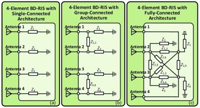
Figure 1: Schematic circuit topologies for a 4-element BD-RIS with (a) single-connected, (b) group-connected, and (c) fully-connected architectures.

In addition, we assume that each transmit antenna is connected in series with a voltage source and a source impedance, yielding a source impedance matrix $\mathbf{Z}_{T}\in\mathbb{C}^{N\times N}$. Accordingly, the reflection coefficient matrix at the transmitter is $\mathbf{\Gamma}_{T}=(\mathbf{Z}_{T}+Z_{0}\mathbf{I}_{N})^{-1}(\mathbf{Z}_{T}-Z_{0}\mathbf{I}_{N})$, where $Z_{0}$ is the reference impedance used to calculate the scattering matrix. Similarly, each receive antenna is connected to the ground through a load impedance, yielding a load impedance matrix $\mathbf{Z}_{R}\in\mathbb{C}^{K\times K}$ and a reflection coefficient matrix $\mathbf{\Gamma}_{R}=(\mathbf{Z}_{R}+Z_{0}\mathbf{I}_{K})^{-1}(\mathbf{Z}_{R}-Z_{0}\mathbf{I}_{K})$. The $M$ scattering elements at the BD-RIS are connected to an $M$-port group-connected reconfigurable impedance network [2], where the $M$ ports are uniformly divided into $G$ groups, each containing $\bar{M}=\frac{M}{G}$ ports connected to each other. Mathematically, BD-RIS with a group-connected architecture is characterized by a block-diagonal impedance matrix $\mathbf{Z}_{I}\in\mathbb{C}^{M\times M}$, i.e.,

$$\mathbf{Z}_{I}=\mathsf{blkdiag}(\mathbf{Z}_{I,1},\ldots,\mathbf{Z}_{I,G}),$$ (1)

where each block $\mathbf{Z}_{I,g}\in\mathbb{C}^{\bar{M}\times\bar{M}}$, $\forall g\in\mathcal{G}=\{1,\ldots,G\}$, is symmetric and purely imaginary for reciprocal and lossless reconfigurable impedance networks [2], i.e.,

$$\mathbf{Z}_{I,g}=\mathbf{Z}_{I,g}^{T},~{}\Re\{\mathbf{Z}_{I,g}\}=\mathbf{0},\forall g\in\mathcal{G}.$$ (2)

Specifically, the cases with $G=1$ and $G=M$ refer to the fully- and single-connected architectures of BD-RIS [2], where the corresponding impedance matrices become full matrices and diagonal matrices, respectively. To facilitate understanding, we provide the schematic circuit topologies of BD-RIS with single-, group-, and fully-connected architectures in Fig. 1. The impedance matrix in (2) results in a symmetric and unitary matrix $\mathbf{\Theta}\in\mathbb{C}^{M\times M}$ of reflection coefficients with

$$\mathbf{\Theta}=(\mathbf{Z}_{I}+Z_{0}\mathbf{I}_{M})^{-1}(\mathbf{Z}_{I}-Z_{0}\mathbf{I}_{M}).$$ (3)

Using these definitions and multiport network theory based on the scattering parameters, the general RIS aided channel, $\mathbf{H}\in\mathbb{C}^{K\times N}$, which relates the voltage at the receiver ports with those at transmitter ports, is given by[2]

$$\mathbf{H}=(\mathbf{\Gamma}_{R}+\mathbf{I}_{K})^{-1}\mathbf{T}_{RT}(\mathbf{I}_{N}+\mathbf{\Gamma}_{T}\mathbf{T}_{TT}+\mathbf{T}_{TT})^{-1},$$ (4)

where $\mathbf{T}_{TT}\in\mathbb{C}^{N\times N}$ and $\mathbf{T}_{RT}\in\mathbb{C}^{K\times N}$ are sub-matrices of $\mathbf{T}=\mathbf{S}(\mathbf{I}_{L}-\mathbf{\Gamma}\mathbf{S})^{-1}\in\mathbb{C}^{L\times L}$ with $\mathbf{\Gamma}=\mathsf{blkdiag}(\mathbf{\Gamma}_{T},\mathbf{\Theta},\mathbf{\Gamma}_{R})$. Specifically, $\mathbf{T}_{TT}=[\mathbf{T}]_{1:N,1:N}$ and $\mathbf{T}_{RT}=[\mathbf{T}]_{N+M+1:L,1:N}$. The channel model in (4) is general enough to include the impact of antenna mismatching and mutual coupling at the transmitter, BD-RIS, and receiver. However, it is too complicated to get insights on the role of BD-RIS, which motivates us to apply further simplifications.

II-B Mutual Coupling Aware RIS Aided Communication Model

To simplify the general communication model (4), we introduce the impedance matrix $\mathbf{Z}\in\mathbb{C}^{L\times L}$ for the whole $L$-port network, which can be formulated in terms of sub-matrices, as $\mathbf{Z}=[\mathbf{Z}_{TT},\mathbf{Z}_{TI},\mathbf{Z}_{TR};\mathbf{Z}_{IT},\mathbf{Z}_{II},\mathbf{Z}_{IR};\mathbf{Z}_{RT},\mathbf{Z}_{RI},\mathbf{Z}_{RR}]$. Then, we make the following assumptions.

Assumption 1: The source impedances at the transmitter and the load impedances at the receiver are equal to the reference impedance $Z_{0}$, i.e., $\mathbf{Z}_{T}=Z_{0}\mathbf{I}_{N}$ and $\mathbf{Z}_{R}=Z_{0}\mathbf{I}_{K}$, such that $\mathbf{\Gamma}_{T}=\mathbf{0}$ and $\mathbf{\Gamma}_{R}=\mathbf{0}$. This corresponds to the best power matching at the transmitter and receiver, respectively.

Assumption 2 (Unilateral Approximation): The distances between the transmitter and receiver, transmitter and BD-RIS, and BD-RIS and receiver are sufficiently large such that the links from receiving devices to transmitting devices are negligible, i.e., $\mathbf{Z}_{TI}\approx\mathbf{0}$, $\mathbf{Z}_{TR}\approx\mathbf{0}$, $\mathbf{Z}_{IR}\approx\mathbf{0}$.

Assumption 3: The antennas at the transmitter and receiver are perfectly matched with no mutual coupling, such that $\mathbf{Z}_{TT}=Z_{0}\mathbf{I}_{N}$ and $\mathbf{Z}_{RR}=Z_{0}\mathbf{I}_{K}$.

Based on Assumptions 2 and 3, and the relationship $\mathbf{S}=(\mathbf{Z}+Z_{0}\mathbf{I}_{L})^{-1}(\mathbf{Z}-Z_{0}\mathbf{I}_{L})$, we obtain the following result.

Result 1: The transmission scattering matrices from the receiver to the transmitter are zero, i.e., $\mathbf{S}_{TI}\approx\mathbf{0}$, $\mathbf{S}_{TR}\approx\mathbf{0}$, $\mathbf{S}_{IR}\approx\mathbf{0}$. The scattering matrices at the antenna arrays of the transmitter and receiver are zero, i.e., $\mathbf{S}_{TT}\approx\mathbf{0}$, $\mathbf{S}_{RR}\approx\mathbf{0}$.

Applying Assumption 1 and Result 1, the expression in (4) can be simplified as follows:

$$\mathbf{H}\approx\mathbf{S}_{RT}+\mathbf{S}_{RI}(\mathbf{I}_{M}-\mathbf{\Theta}\mathbf{S}_{II})^{-1}\mathbf{\Theta}\mathbf{S}_{IT}.$$ (5)

However, (5) is still too complex, since the matrix $\mathbf{\Theta}$ of reflection coefficients appears inside and outside the inverse. To further simplify the expression in (5), so as to facilitate the optimization of BD-RIS in the presence of mutual coupling, we leverage Assumptions 1-3 and the relationship between $\mathbf{S}$ and $\mathbf{Z}$, and obtain the following result.

Result 2: The nonzero sub-matrices of $\mathbf{S}$ and those of $\mathbf{Z}$ are related to one another as follows:

$$\mathbf{S}_{RI} =\frac{\mathbf{Z}_{RI}}{2Z_{0}}(\mathbf{I}_{M}-(\mathbf{Z}_{II}+Z_{0}\mathbf{I}_{M})^{-1}(\mathbf{Z}_{II}-Z_{0}\mathbf{I}_{M})),$$ (6a)

$$\mathbf{S}_{II} =(\mathbf{Z}_{II}+Z_{0}\mathbf{I}_{M})^{-1}(\mathbf{Z}_{II}-Z_{0}\mathbf{I}_{M}),$$ (6b)

$$\mathbf{S}_{IT} =(\mathbf{Z}_{II}+Z_{0}\mathbf{I}_{M})^{-1}\mathbf{Z}_{IT},$$ (6c)

$$\mathbf{S}_{RT} =\frac{\mathbf{Z}_{RT}}{2Z_{0}}-\frac{\mathbf{Z}_{RI}}{2Z_{0}}(\mathbf{Z}_{II}+Z_{0}\mathbf{I}_{M})^{-1}\mathbf{Z}_{IT}.$$ (6d)

Plugging (6) and (3) into (5), we obtain a more tractable and convenient expression equivalent to (5) as

$$\mathbf{H}\approx\frac{1}{2Z_{0}}(\mathbf{Z}_{RT}-\mathbf{Z}_{RI}(\mathbf{Z}_{II}+\mathbf{Z}_{I})^{-1}\mathbf{Z}_{IT}).$$ (7)

Equation (7) is in accordance with the model in [8], which was derived using the impedance parameter analysis. In (7), the role of the beyond-diagonal network of tunable impedances in BD-RIS and the impact of mutual coupling and mismatching at the RIS elements are explicitly visible. The physical meaning of each term in (7) is explained as follows.

1. $\mathbf{Z}_{RT}$, $\mathbf{Z}_{RI}$, and $\mathbf{Z}_{IT}$ refer to the channels from the transmitter to the receiver, from the BD-RIS to the receiver, and from the transmitter to the BD-RIS, respectively.

2. $\mathbf{Z}_{II}$ characterizes the mismatching and mutual coupling at the RIS elements. Specifically, the diagonal entries of $\mathbf{Z}_{II}$ refer to the self impedance; the off-diagonal entries of $\mathbf{Z}_{II}$ account for the mutual coupling, which depends on the inter-element distance. Generally, the larger the inter-element distance, the smaller the mutual coupling.

With the communication model in (7) at hand, which explicitly accounts for the mutual coupling at the BD-RIS, in the following section, we aim to design the beyond-diagonal matrix $\mathbf{Z}_{I}$ of tunable impedances to maximize the system performance.

Remark 1: We clarify that we start from the general channel model derived in [2], but go beyond that by deriving the new expression in (5), which captures explicitly the mutual coupling among the RIS elements. In addition, only the conventional RIS with single-connected architecture is considered in [8], i.e., $\mathbf{Z}_{I}$ is diagonal, while in this work we consider BD-RIS with $\mathbf{Z}_{I}$ not limited to being diagonal. For the first time, more importantly, we show the equivalence between the scattering parameter based channel in (5) and the impedance parameter based channel in (7) derived in [8].

III Mutual Coupling Aware Optimization

For simplicity, we consider a SISO system and focus on the optimization of $\mathbf{Z}_{I}$, which is not limited to being diagonal in BD-RIS. The analysis of the multiple-antenna case is postponed to a future work due to the complexity of considering a joint optimization including the precoder at the transmitter, the beyond-diagonal matrix $\mathbf{Z}_{I}$ at the BD-RIS, and the combiner at the receiver. The corresponding optimization problem to maximize the channel gain can be formulated as

$$\max_{\mathbf{Z}_{I}}{} |z_{RT}-\mathbf{z}_{RI}(\mathbf{Z}_{II}+\mathbf{Z}_{I})^{-1}\mathbf{z}_{IT}|^{2}~{}~{}\mathrm{s.t.}~{}\text{(\ref{eq:z_blkdiag}), (\ref{eq:z_cons})},$$ (8)

where $z_{RT}\in\mathbb{C}$, $\mathbf{z}_{RI}\in\mathbb{C}^{1\times M}$, and $\mathbf{z}_{IT}\in\mathbb{C}^{M\times 1}$. The main difficulties when solving the problem in (8) are the following:

1. The matrix $\mathbf{Z}_{I}$ appears in the inversion $(\mathbf{Z}_{II}+\mathbf{Z}_{I})^{-1}$.

2. The matrix $\mathbf{Z}_{I}$ needs to fulfill the constraints (1) and (2), instead of being diagonal as in conventional RISs.

The first difficulty has been tackled in [9] for diagonal RISs. However, the optimization with mutual coupling among the RIS elements and the unique constraints of BD-RIS have never been investigated. To effectively solve problem (8), we apply the idea introduced in [9] and propose to iteratively optimize $\mathbf{Z}_{I}$ subject to the constraints (1) and (2) until convergence. This results in the following optimization framework.

III-A Optimization Framework

The main idea of the iterative design in [9] is to slightly modify the value of $\mathbf{Z}_{I}$ in each iteration, in order to increase the channel gain. Inspired by this approach, we first introduce an auxiliary variable $\mathbf{\Omega}\in\mathbb{C}^{M\times M}$ as a small increment to $\mathbf{Z}_{I}$ in each iteration. To facilitate the iterative design, we construct $\mathbf{\Omega}$ based on the following two properties.

Property 1: $\mathbf{\Omega}$ is chosen in compliance with the mathematical structure of the impedance matrix $\mathbf{Z}_{I}$, such that the updated impedance matrix always satisfies the optimization constraints in each iteration. Specifically, we have

$$\mathbf{\Omega}=\mathsf{blkdiag}(\mathbf{\Omega}_{1},\ldots,\mathbf{\Omega}_{G}),~{}\mathbf{\Omega}_{g}=\mathbf{\Omega}_{g}^{T},\forall g.$$ (9)

Property 2: Each nonzero entry of $\mathbf{\Omega}$ is chosen sufficiently small, such that the convergence of the optimization framework is guaranteed [9]. For ease of optimization, we assume that each nonzero entry of $\mathbf{\Omega}$ has the same amplitude but a different phase, i.e.,

$$|[\mathbf{\Omega}_{g}]_{m,n}|=\delta,\forall g,\forall m,n\in\bar{\mathcal{M}}=\{1,\ldots,\bar{M}\},$$ (10)

where $\delta$ controls the increment of $\mathbf{Z}_{I}$ in each iteration, which is explained in details in the following subsection.

Based on these two properties for $\mathbf{\Omega}$, the proposed iterative design is summarized by the following steps.

Step 1: At the $l$-th iteration, we optimize $\mathbf{\Omega}^{l}$, while keeping $\mathbf{Z}_{I}^{l}$ fixed, by solving the following problem:

$$\max_{\mathbf{\Omega}}{} |z_{RT}-\mathbf{z}_{RI}(\mathbf{Z}_{II}+\mathbf{Z}_{I}^{l}+\mathbf{\Omega})^{-1}\mathbf{z}_{IT}|^{2}~{}~{}\mathrm{s.t.}~{}\text{(\ref{eq:omega_blkdiag}), (\ref{eq:omega_cons})}.$$ (11)

Step 2: Given $\mathbf{\Omega}^{l}$ as the optimal solution to the problem in (11), the impedance matrix at the $(l+1)$-th iteration, i.e., $\mathbf{Z}_{I}^{l+1}$, is updated using the following rule:

$$\mathbf{Z}_{I}^{l+1}=\mathbf{Z}_{I}^{l}+j\Im\{\mathbf{\Omega}^{l}\},$$ (12)

where we only use the imaginary part of $\mathbf{\Omega}^{l}$ to guarantee that the impedance matrix is purely imaginary.

Then, $\mathbf{Z}_{I}$ is optimized by iteratively solving the problem in (11) and updating (12) until convergence. The solution of the problem in (11) is detailed next.

III-B Solution to Problem (11)

In (11), instead of optimizing $\mathbf{Z}_{I}$ as in (8), we optimize the small increment $\mathbf{\Omega}$, such that $\mathbf{\Omega}$ can be removed from the matrix inversion in the objective function. Specifically, we apply the Neumann series approximation [9] to matrix inversion, i.e., $(\mathbf{Z}_{II}+\mathbf{Z}_{I}^{l}+\mathbf{\Omega})^{-1}\approx(\mathbf{Z}_{II}+\mathbf{Z}_{I}^{l})^{-1}-(\mathbf{Z}_{II}+\mathbf{Z}_{I}^{l})^{-1}\mathbf{\Omega}(\mathbf{Z}_{II}+\mathbf{Z}_{I}^{l})^{-1}$, which achieves a tight approximation provided that the condition $\delta\ll\frac{1}{\bar{M}\|(\mathbf{Z}_{II}+\mathbf{Z}_{I}^{l})^{-1}\|_{\infty}}$ is fulfilled in each iteration. Accordingly, we have $|z_{RT}-\mathbf{z}_{RI}(\mathbf{Z}_{II}+\mathbf{Z}_{I}^{l}+\mathbf{\Omega})^{-1}\mathbf{z}_{IT}|^{2}\approx|a^{l}+\mathbf{b}^{l}\mathbf{\Omega}\mathbf{c}^{l}|^{2}=|a^{l}+\sum_{g\in\mathcal{G}}\mathbf{e}_{g}^{l}\mathsf{vec}(\mathbf{\Omega}_{g})|^{2}$, where $a^{l}=z_{RT}-\mathbf{z}_{RI}(\mathbf{Z}_{II}+\mathbf{Z}_{I}^{l})^{-1}\mathbf{z}_{IT}$, $\mathbf{b}^{l}=\mathbf{z}_{RI}(\mathbf{Z}_{II}+\mathbf{Z}_{I}^{l})^{-1}$, $\mathbf{c}^{l}=(\mathbf{Z}_{II}+\mathbf{Z}_{I}^{l})^{-1}\mathbf{z}_{IT}$, $\mathbf{b}_{g}^{l}=[\mathbf{b}^{l}]_{(g-1)\bar{M}+1:g\bar{M}}$, $\mathbf{c}_{g}^{l}=[\mathbf{c}^{l}]_{(g-1)\bar{M}+1:g\bar{M}}$, and $\mathbf{e}_{g}^{l}=(\mathbf{c}_{g}^{l})^{T}\otimes\mathbf{b}_{g}^{l}$, $\forall g\in\mathcal{G}$. As a result, the problem in (11) becomes

$$\max_{\mathbf{\Omega}_{g},\forall g}{} \Big{|}a^{l}+\sum_{g\in\mathcal{G}}\mathbf{e}_{g}^{l}\mathsf{vec}(\mathbf{\Omega}_{g})\Big{|}^{2}~{}~{}\mathrm{s.t.}~{}\mathbf{\Omega}_{g}=\mathbf{\Omega}_{g}^{T},\text{(\ref{eq:omega_cons})}.$$ (13)

The solution to the problem in (13) is not straightforward due to the symmetric and constant modulus constraints of $\mathbf{\Omega}_{g},\forall g$. Fortunately, the symmetric constraint of each $\mathbf{\Omega}_{g}$ implies that we do not need to optimize the whole matrices $\mathbf{\Omega}_{g},\forall g$. In other words, instead of optimizing the symmetric matrices $\mathbf{\Omega}_{g},\forall g$ with $\bar{M}^{2}$ variables, we can optimize $\bar{M}$ diagonal variables and $\frac{\bar{M}(\bar{M}-1)}{2}$ lower-triangular (or upper-triangular) variables of $\mathbf{\Omega}_{g}$, and reconstruct them to obtain $\mathbf{\Omega}_{g},\forall g$. Mathematically, this transformation can be done by introducing the following notations.

1. A column vector $\bm{\omega}_{g}\in\mathbb{C}^{\frac{\bar{M}(\bar{M}+1)}{2}\times 1}$, which contains the diagonal and lower-triangular entries of $\mathbf{\Omega}_{g}$.

2. A binary matrix $\mathbf{P}\in\{0,1\}^{\bar{M}^{2}\times\frac{\bar{M}(\bar{M}+1)}{2}}$, which maps $\bm{\omega}_{g}$ into $\mathsf{vec}(\mathbf{\Omega}_{g}),\forall g$.

Specifically, there is only one nonzero entry in each row of the binary matrix $\mathbf{P}$, which is defined as

$$[\mathbf{P}]_{\bar{M}(m-1)+n,k}=\begin{cases}1,&k=\frac{m(m-1)}{2}+n~{}\text{and}~{}1\leq n\leq m,\\ 1,&k=\frac{n(n-1)}{2}+m~{}\text{and}~{}m<n\leq\bar{M},\\ 0,&\text{otherwise},\end{cases}$$ (14)

where $\forall m,n\in\bar{\mathcal{M}}$. Accordingly, we obtain the relationship $\mathsf{vec}(\mathbf{\Omega}_{g})=\mathbf{P}\bm{\omega}_{g},\forall g$, and the problem in (13) becomes

$$\max_{\bm{\omega}_{g},\forall g}{} \Big{|}a^{l}+\sum_{g\in\mathcal{G}}\mathbf{e}_{g}^{l}\mathbf{P}\bm{\omega}_{g}\Big{|}^{2}~{}~{}\mathrm{s.t.}~{}|[\bm{\omega}_{g}]_{i}|=\delta,\forall g,\forall i\in\ddot{\mathcal{M}},$$ (15)

where $\ddot{\mathcal{M}}\in\{1,\ldots,\frac{\bar{M}(\bar{M}+1)}{2}\}$. Applying the triangle inequality to the objective function in (15), we have $|a^{l}+\sum_{g\in\mathcal{G}}\mathbf{e}_{g}^{l}\mathbf{P}\bm{\omega}_{g}|\leq|a^{l}|+\delta\sum_{g\in\mathcal{G}}\sum_{i\in\ddot{\mathcal{M}}}|[\mathbf{e}_{g}^{l}\mathbf{P}]_{i}|$, where the equality is achieved by rotating each $[\mathbf{e}_{g}^{l}\mathbf{P}]_{i}$ such that the resulting $[\mathbf{e}_{g}^{l}\mathbf{P}]_{i}[\bm{\omega}_{g}]_{i}$, $\forall i$, are collinear to $a^{l}$ on the complex plane. Therefore, the optimal solution of $\bm{\omega}_{g}$, $\forall g$ in the $l$-th iteration can be determined element-by-element as

$$[\bm{\omega}_{g}^{l}]_{i}=\delta\exp(j(\angle a^{l}-\angle[\mathbf{e}_{g}^{l}\mathbf{P}]_{i})),\forall i.$$ (16)

With the solution in (16), we can reconstruct $\mathbf{\Omega}_{g}$ in the $l$-th iteration by $\mathbf{\Omega}_{g}^{l}=\overline{\mathsf{vec}}(\mathbf{P}\bm{\omega}_{g}^{l})$, $\forall g$.

Remark 2: The approach proposed in this letter is different from that in [9] from two perspectives. First, we introduce the auxiliary variable $\mathbf{\Omega}$ with the unique constraint in (9) based on BD-RIS architectures, instead of being diagonal as in conventional RISs. Second, we introduce the binary matrix $\mathbf{P}$ to deal with the symmetric constraint of $\mathbf{\Omega}$ and to further facilitate the optimization.

III-C Summary and Analysis

III-C.1 Algorithm

The complete algorithm for solving the problem in (8) corresponds to the following steps:

1. Initialize $\mathbf{Z}_{I}^{0}$ by solving problem (8) considering the conventional diagonal RIS with no mutual coupling, $\mathbf{\Omega}^{0}=\mathbf{0}$, and $l=0$. Calculate $a^{0}$, $\mathbf{b}^{0}$, and $\mathbf{c}^{0}$.

2. Update $l=l+1$.

3. Update $\mathbf{Z}_{I}^{l}$ using (12), $a^{l}$, $\mathbf{b}^{l}$, and $\mathbf{c}^{l}$.

4. Update $\bm{\omega}_{g}^{l}$, $\forall g$ using (16), and $\mathbf{\Omega}_{g}^{l}=\overline{\mathsf{vec}}(\mathbf{P}\bm{\omega}_{g}^{l})$, $\forall g$.

5. Calculate $C^{l}=|a^{l}+\mathbf{b}^{l}j\Im\{\mathbf{\Omega}^{l}\}\mathbf{c}^{l}|^{2}$.

6. Repeat S2-S5 until the value of $C^{l}$ converges.

III-C.2 Complexity

The complexity of the proposed algorithm mainly comes from the matrix inversion operation for updating $a^{l}$, $\mathbf{b}^{l}$, and $\mathbf{c}^{l}$, which requires $\mathcal{O}(M^{3})$ complex multiplications. Therefore, the total complexity is $\mathcal{O}(IM^{3})$, where $I$ denotes the number of iterations to ensure convergence.

III-C.3 Convergence

The convergence of the proposed algorithm is theoretically guaranteed by appropriately setting the value of $\delta$. Specifically, we have the relationship $C^{l}=|a^{l}+\mathbf{b}^{l}j\Im\{\mathbf{\Omega}^{l}\}\mathbf{c}^{l}|^{2}=|a^{l}+j\sum_{g\in\mathcal{G}}\mathbf{e}_{g}^{l}\mathbf{P}\Im\{\bm{\omega}_{g}\}|^{2}\overset{\text{(a)}}{=}|j\delta\sum_{g}\sum_{i}|[\mathbf{e}_{g}^{l}\mathbf{P}]_{i}|\sin(\angle a^{l}-\angle[\mathbf{e}_{g}^{l}\mathbf{P}]_{i})\cos(\angle a^{l}-\angle[\mathbf{e}_{g}^{l}\mathbf{P}]_{i})+|a^{l}|+\delta\sum_{g}\sum_{i}|[\mathbf{e}_{g}^{l}\mathbf{P}]_{i}|\sin^{2}(\angle a^{l}-\angle[\mathbf{e}_{g}^{l}\mathbf{P}]_{i})|^{2}\geq|a^{l}|^{2}=|z_{RT}-\mathbf{z}_{RI}(\mathbf{Z}_{II}+\mathbf{Z}_{I}^{l})^{-1}\mathbf{z}_{IT}|^{2}=|z_{RT}-\mathbf{z}_{RI}(\mathbf{Z}_{II}+\mathbf{Z}_{I}^{l-1}+j\Im\{\mathbf{\Omega}^{l-1}\})^{-1}\mathbf{z}_{IT}|^{2}\overset{\text{(b)}}{\approx}|a^{l-1}+\mathbf{b}^{l-1}j\Im\{\mathbf{\Omega}^{l-1}\}\mathbf{c}^{l-1}|^{2}=C^{l-1}$, where (a) follows by plugging (16) into $C^{l}$; (b) follows from the Neumann series approximation. Therefore, we have $C^{l}\geq|a^{l}|^{2}\approx C^{l-1}$, which proves that the objective function $C^{l}$ is monotonically non-decreasing after each iteration. Therefore, we conclude that the proposed algorithm converges since the value of the objective function $C^{l}$ is bounded from above.

IV Performance Evaluation

In this section, we perform simulation results to evaluate the performance of the proposed algorithm. The simulation parameters are the same as in [9] and are summarized as follows. Free-space propagation is assumed. The transmitter and receiver are located at (5,-5,3) and (5,5,1), respectively. BD-RIS is located on the $y$-$z$ plane and is centered at (0,0,0). All the radiating elements are thin dipoles that are parallel to the $z$-axis and have radius $r=\frac{\lambda}{500}$ and length $\iota=\frac{\lambda}{32}$, where $\lambda=\frac{c}{f}$ denotes the wavelength with frequency $f=28$ GHz. Thus, the mutual impedance between any two dipoles $a$ and $b$ with center-point coordinates $(a_{x},a_{y},a_{z})$ and $(b_{x},b_{y},b_{z})$ (and the self impedance at any dipole if $a=b$) is computed as [8]

$$z_{a,b} =\int_{a_{z}-\frac{\iota}{2}}^{a_{z}+\frac{\iota}{2}}\int_{b_{z}-\frac{\iota}{2}}^{b_{z}+\frac{\iota}{2}}\frac{j\eta_{0}}{4\pi\kappa_{0}}\bigg{(}\frac{(a_{z}^{\prime}-b_{z}^{\prime})^{2}}{d_{a,b}^{2}}\big{(}\frac{3}{d_{a,b}^{2}}+\frac{j3\kappa_{0}}{d_{a,b}}$$ (17)

$$~{}-\kappa_{0}^{2}\big{)}-\frac{j\kappa_{0}d_{a,b}+d_{a,b}^{-1}}{d_{a,b}}+\kappa_{0}^{2}\bigg{)}\frac{\exp(-j\kappa_{0}d_{a,b})}{d_{a,b}}$$

$$~{}\times\frac{\sin(\kappa_{0}(\frac{\iota}{2}-|b_{z}^{\prime}-b_{z}|))\sin(\kappa_{0}(\frac{\iota}{2}-|a_{z}^{\prime}-a_{z}|))}{\sin^{2}(\kappa_{0}\frac{\iota}{2})}db_{z}^{\prime}da_{z}^{\prime},$$

where $\eta_{0}=377$ $\Omega$ denotes the characteristic impedance, $\kappa_{0}=\frac{2\pi}{\lambda}$ is the wavenumber, and $d_{a,b}$ denotes the distance between the dipoles $a$ and $b$, i.e., $d_{a,b}=\sqrt{(d_{a,b}^{x,y})^{2}+(a_{z}^{\prime}-b_{z}^{\prime})^{2}}$, $d_{a,b}^{x,y}=\sqrt{(a_{x}-b_{x})^{2}+(a_{y}-b_{y})^{2}}$ for $a\neq b$ and $d_{a,b}^{x,y}=r$ for $a=b$. The elements of $\mathbf{z}_{RI}$, $\mathbf{Z}_{II}$, and $\mathbf{z}_{IT}$ are computed using (17), and we set $z_{RT}=0$ to focus on the role of BD-RIS.

Figure 2: Channel gain versus the number of iterations ($M=16$).

Figure 3: Channel gain versus the number of BD-RIS elements.

Fig. 2 evaluates the convergence of the proposed algorithm for different inter-element distance $d$ and for different BD-RIS architectures. The schemes marked as “FC/GC/SC” refer to the performance achieved by BD-RIS with fully/group/single-connected architectures. We set $\bar{M}=4$ for the group-connected case. The value of $\delta$ is set to $6\times 10^{-4}$ to ensure convergence. We observe that the proposed algorithm converges, which verifies our theoretical derivation. In addition, we observe that, when the number of RIS elements is fixed, the end-to-end channel gain decreases when decreasing inter-element distance due to the increased mutual coupling. When the aperture (size) of the RIS is kept fixed, on the other hand, a smaller inter-element distance enables the deployment of more RIS elements within the surface, which results in better beamforming gains provided that the mutual coupling is considered in the RIS design [9].

Fig. 3 illustrates the channel gain of BD-RIS with different architectures and different inter-element distances. In Fig. 3, the schemes marked as “w/ MC” are obtained by computing $\mathbf{Z}_{I}$ with $\mathbf{Z}_{II}$ using (17); the schemes marked as “w/o MC” are obtained by setting the off-diagonal entries of $\mathbf{Z}_{II}$ to zero. In both cases, the channel gain is $|\mathbf{z}_{RI}(\mathbf{Z}_{II}+\mathbf{Z}_{I})^{-1}\mathbf{z}_{IT}|^{2}$. We have the following observations. First, ignoring the mutual coupling when designing $\mathbf{Z}_{I}$, BD-RIS with single/group/fully-connected architectures achieves exactly the same performance, which is consistent with the conclusion in [2]. Second, by taking into account the mutual coupling when designing $\mathbf{Z}_{I}$, BD-RIS with different architectures achieves better performance than the “w/o MC” schemes. Third, the performance gap between fully/group-connected BD-RIS and conventional RIS increases when decreasing the inter-element distance. This can be attributed to the impact of mutual coupling, which becomes more prominent when decreasing the inter-element distance. This, in fact, results in larger values for the off-diagonal entries of $\mathbf{Z}_{II}$, which is better exploited by BD-RIS architectures for performance improvement.

V Conclusion

In this work, we studied the modeling and optimization of BD-RIS aided wireless communication systems in the presence of mutual coupling among the RIS elements. Specifically, we first derived the mutual coupling aware BD-RIS aided wireless communication model based on scattering parameter and impedance parameter analysis, showing their equivalence. We then proposed a general algorithm to maximize the channel gain of BD-RIS for SISO systems. We finally illustrated simulation results to analyze the effectiveness of the proposed design and the impact of mutual coupling on BD-RIS architectures. The numerical results show that the larger the mutual coupling the larger the gain offered by BD-RIS.

References

- [1] Q. Wu, S. Zhang, B. Zheng, C. You, and R. Zhang, “Intelligent reflecting surface-aided wireless communications: A tutorial,” IEEE Trans. Commun., vol. 69, no. 5, pp. 3313–3351, 2021.
- [2] S. Shen, B. Clerckx, and R. Murch, “Modeling and architecture design of reconfigurable intelligent surfaces using scattering parameter network analysis,” IEEE Trans. Wireless Commun., vol. 21, no. 2, pp. 1229–1243, 2022.
- [3] H. Li, S. Shen, M. Nerini, and B. Clerckx, “Reconfigurable intelligent surfaces 2.0: Beyond diagonal phase shift matrices,” IEEE Commun. Mag., 2023.
- [4] H. Zhang and B. Di, “Intelligent omni-surfaces: Simultaneous refraction and reflection for full-dimensional wireless communications,” IEEE Comm. Surveys & Tutorials, 2022.
- [5] Q. Li, M. El-Hajjar, I. A. Hemadeh, A. Shojaeifard, A. Mourad, B. Clerckx, and L. Hanzo, “Reconfigurable intelligent surfaces relying on non-diagonal phase shift matrices,” IEEE Trans. Veh. Technol., vol. 71, no. 6, pp. 6367–6383, 2022.
- [6] M. Nerini, S. Shen, H. Li, and B. Clerckx, “Beyond diagonal reconfigurable intelligent surfaces utilizing graph theory: Modeling, architecture design, and optimization,” arXiv preprint arXiv:2305.05013, 2023.
- [7] M. Di Renzo, F. H. Danufane, and S. Tretyakov, “Communication models for reconfigurable intelligent surfaces: From surface electromagnetics to wireless networks optimization,” Proc. IEEE, vol. 110, no. 9, pp. 1164–1209, 2022.
- [8] G. Gradoni and M. Di Renzo, “End-to-end mutual coupling aware communication model for reconfigurable intelligent surfaces: An electromagnetic-compliant approach based on mutual impedances,” IEEE Wireless Commun. Lett., vol. 10, no. 5, pp. 938–942, 2021.
- [9] X. Qian and M. Di Renzo, “Mutual coupling and unit cell aware optimization for reconfigurable intelligent surfaces,” IEEE Wireless Commun. Lett., vol. 10, no. 6, pp. 1183–1187, 2021.
- [10] M. T. Ivrlač and J. A. Nossek, “Toward a circuit theory of communication,” IEEE Trans. Circuits Syst. I, Reg. Papers, vol. 57, no. 7, pp. 1663–1683, 2010.