Tackling Hybrid Heterogeneity on Federated Optimization via
Gradient Diversity Maximization

Abstract

Federated learning refers to a distributed machine learning paradigm in which data samples are decentralized and distributed among multiple clients. These samples may exhibit statistical heterogeneity, which refers to data distributions are not independent and identical across clients. Additionally, system heterogeneity, or variations in the computational power of the clients, introduces biases into federated learning. The combined effects of statistical and system heterogeneity can significantly reduce the efficiency of federated optimization. However, the impact of hybrid heterogeneity is not rigorously discussed. This paper explores how hybrid heterogeneity affects federated optimization by investigating server-side optimization. The theoretical results indicate that adaptively maximizing gradient diversity in server update direction can help mitigate the potential negative consequences of hybrid heterogeneity. To this end, we introduce a novel server-side gradient-based optimizer FedAWARE with theoretical guarantees provided. Intensive experiments in heterogeneous federated settings demonstrate that our proposed optimizer can significantly enhance the performance of federated learning across varying degrees of hybrid heterogeneity.

1 Introduction

We study a standard cross-device federated learning (FL) task (Kairouz et al., 2021), which minimizes a finite sum of local empirical objectives:

$$\min_{\boldsymbol{x}\in\mathcal{X}}f(\boldsymbol{x}):=\sum_{i=1}^{N}\lambda_{i}f_{i}(\boldsymbol{x}):=\sum_{i=1}^{N}\lambda_{i}\mathbb{E}_{\xi_{i}\sim\mathcal{D}_{i}}[F_{i}(\boldsymbol{x},\xi_{i})],$$ (1)

where $\boldsymbol{x}\in\mathcal{X}\subseteq\mathbb{R}^{d}$ is parameters of machine learning model, $f(\boldsymbol{x})$ is the global objective weighted by $\lambda\in\mathbb{R}^{N}$, $\xi_{i}$ is stochastic batch data, and $\mathcal{D}_{i}$ denotes dataset on the $i$-th client ($i\in\{1,2,\ldots,N$}). The federated optimization framework that minimizes the global objective can be summarized into client optimization and server optimization procedures, as shown in Figure 1. Take the FedAvg (McMahan et al., 2017) as a example:

$$\underbrace{\boldsymbol{x}^{t+1}-\boldsymbol{x}^{t}=-\eta\sum_{i=1}^{N}\lambda_{i}\boldsymbol{g}_{i}^{t}}_{\text{Server Opt.}}=-\sum_{i=1}^{N}\lambda_{i}\cdot\underbrace{\eta_{l}\sum_{k=0}^{K_{i}-1}\nabla F_{i}(\boldsymbol{x}_{i}^{t,k})}_{\text{Client Opt.}},$$ (2)

where we use $\nabla F_{i}(\boldsymbol{x})$ to denote stochastic gradients over a mini-batch of samples, $\boldsymbol{x}_{i}^{t,k}$ to denote client $i$’s model after the $k$ local update steps at the $t$-th communication round and $\boldsymbol{g}_{i}^{t}=\boldsymbol{x}_{i}^{t,K_{i}}-\boldsymbol{x}_{i}^{t,0}$ to denote the local updates made by client $i$ at round $t$. Also, $\eta_{l}$ is the client learning rate. However, federated optimization suffers from two major optimization challenges (Li et al., 2020b, c).

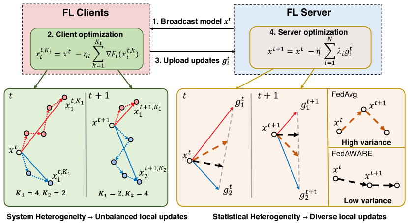
Figure 1: Example of federated optimization framework and challenges. System heterogeneity induces unbalanced local updates and hence enlarges the statistical heterogeneity impacts on server optimization. We propose a server-side optimizer FedAWARE to tackle the challenges without manipulating local updates.

First, statistical heterogeneity, also known as the non-identically and independently distributed (Non-IID) data problem, is a crucial challenge in FL. This problem arises from the fact that data is non-identically distributed among devices, which can increase the variance of global updates and result in unstable convergence quality and poor generalization performance. To address this challenge, several federated optimization approaches have been proposed. For example, introducing control variates (Karimireddy et al., 2020), momentum terms (Hsu et al., 2019; Reddi et al., 2020), dynamic regularization (Acar et al., 2020), or local penalty terms (Li et al., 2020c) to stabilize global updates have been found effective.

Second, system heterogeneity is another critical challenge in FL. FL involves training models on decentralized devices with varying hardware specifications, operating systems, and software configurations (Imteaj et al., 2021). This can result in communication overheads, computational disparities, and bias. Consequently, faster clients may perform more local updates than slower clients within a fixed wall-clock time interval, resulting in unbalanced local updates. The unbalanced local update steps further negatively impact the federated optimization. To address this issue, FedProx (Li et al., 2020c) proposes using local penalty terms to balance the local updates $\boldsymbol{g}_{i}$. Additionally, FedNova (Wang et al., 2020) clips the local updates $\boldsymbol{g}_{i}$ based on the local update steps $K_{i}$ to maintain objective consistency.

The federated optimization framework face significant challenges from statistical and system heterogeneity, we intend to explore the impacts of hybrid heterogeneity on federated optimization. Previous works (Karimireddy et al., 2020; McMahan et al., 2017; Reddi et al., 2020) often assume that the number of local updates is constant and balanced across all clients $K_{i}=K_{j},\forall i,j\in[N]$, thereby overlooking system heterogeneity. However, statistical and system heterogeneity are often present simultaneously in practice, thereby breaking the assumptions of federated optimization methods. Meanwhile, we note that existing FL algorithms (Li et al., 2020c; Wang et al., 2020) mainly rely on manipulating client-side optimization. However, the impact of hybrid heterogeneity on server-side optimization is not fully discussed.

Observing the facts above, it is natural to ask Are these federated optimization methods still robust to the hybrid heterogeneity challenges? If not, how do the statistical and system heterogeneity hinder the federated optimization performance? We answer these questions by analyzing hybrid heterogeneity from the perspective of server-side optimization. In this paper, we consider clients running vanilla local SGD with heterogeneous data distributions and unbalanced local update steps. Then, we investigate federated server-side optimization within general non-convex settings that encounter such hybrid heterogeneity challenges. The key contributions of this paper are as follows:

• Theoretical Insight: Our theoretical results provide a fascinating insight that gradient diversity is positively correlated with improved solutions in heterogeneous federated optimization. In other words, stationary points with higher gradient diversity tend to achieve better testing accuracy. This finding contradicts previous works that implicitly considered gradient diversity as a negative factor in federated optimization.

• Proposed Method: We introduce a novel server-side gradient-based federated optimization method called Federated Adaptive Weighted AggREgator (FedAWARE). We provide theoretical proof that FedAWARE effectively mitigates hybrid heterogeneity by converging to stationary points with high gradient diversity.

• Evaluation Experiments: We design three different degrees of hybrid heterogeneity settings to assess the ability of existing optimization algorithms. Through evaluation experiments, we demonstrate that FedAWARE consistently outperforms baseline optimization algorithms.

2 Related Work and Preliminaries

Plenty of studies have been proposed to address statistical heterogeneity issues in the FL literature (Ma et al., 2022), including multi-task federated learning (Marfoq et al., 2021; Smith et al., 2017), personalized federated learning (Tan et al., 2022; Liu et al., 2023), knowledge distillation (Zhu et al., 2021; Li & Wang, 2019), and client clustering (Sattler et al., 2020; Zeng et al., 2023a, 2022). In contrast, this paper primarily focuses on federated optimization algorithms that train a robust global model against heterogeneity issues.

The pioneering federated optimization algorithm, FedAvg (McMahan et al., 2017), significantly reduces communication costs. Subsequent works built upon FedAvg to address challenges related to convergence guarantees and heterogeneity issues. For example, some approaches introduced a regularization term in the client objectives (Li et al., 2020c), while others incorporated server momentum (Hsu et al., 2019). Several studies have analyzed the convergence rate of FedAvg and demonstrated its degradation with system heterogeneity (Li et al., 2020c; Wang et al., 2019) and statistical heterogeneity (Zhao et al., 2018; Khaled et al., 2019). SCAFFOLD (Karimireddy et al., 2020) utilizes control variates to mitigate client drift and achieve convergence rates independent of the level of heterogeneity. FedNova (Wang et al., 2020) addresses objective inconsistency issues arising from system heterogeneity through local update regularization. For more detailed comparisons, we refer to the survey (Kairouz et al., 2021). Besides, adaptive methods (Zaheer et al., 2018; Reddi et al., 2019; Xie et al., 2019) have proven to be effective in non-convex optimizations. In the context of federated optimization, FedYogi (Reddi et al., 2020; Zaheer et al., 2018) is a representative adaptive federated optimization algorithm that incorporates Adam-like momentum and adaptive terms to address heterogeneity issues. These related works demonstrate the ongoing efforts to address heterogeneity issues in FL, with various approaches focusing on different aspects of the problem.

Settings. To denote system heterogeneity, we allow the number of local steps $K_{i},i\in[N]$ is not necessarily equal. We denote $[N]=\{1,\dots,N\}$. Then, the central server may only randomly select a subset of clients to perform computation at each round. Furthermore, we consider the clients to be black boxes to the FL server to satisfy privacy-preserving needs (Zhang et al., 2023; Voigt & Von dem Bussche, 2017). In this scenario, clients typically run vanilla SGD locally but can execute any number of local training steps and only upload their updates, while the FL server only accesses the uploaded local updates.

Besides, our non-convex analyses rely on assumptions on local objectives $f_{i}(\boldsymbol{x}),i\in[N]$.

Assumption 2.1 (Smothness).

Each objective $f_{i}(\boldsymbol{x})$ for all $i\in[N]$ is $L$-smooth, inducing that for all $\forall\boldsymbol{x},\boldsymbol{y}\in\mathbb{R}^{d}$, it holds $\|\nabla f_{i}(\boldsymbol{x})-\nabla f_{i}(\boldsymbol{y})\|\leq L\|\boldsymbol{x}-\boldsymbol{y}\|$.

Assumption 2.2 (Unbiasedness and Bounded Local Variance).

For each $i\in[N]$ and $\boldsymbol{x}\in\mathbb{R}^{d}$, we assume the access to an unbiased stochastic gradient $\nabla F_{i}(\boldsymbol{x},\xi_{i})$ of client’s true gradient $\nabla f_{i}(\boldsymbol{x})$, i.e.,$\mathbb{E}_{\xi_{i}\sim\mathcal{D}_{i}}\left[\nabla F_{i}(\boldsymbol{x},\xi_{i})\right]=\nabla f_{i}(\boldsymbol{x})$. The function $f_{i}$ have $\sigma_{l}$-bounded (local) variance i.e.,$\mathbb{E}_{\xi_{i}\sim\mathcal{D}_{i}}\left[\left\|\nabla F_{i}(\boldsymbol{x},\xi_{i})-\nabla f_{i}(\boldsymbol{x})\right\|^{2}\right]\leq\sigma_{l}^{2}$.

3 Analyses on Hybrid Heterogeneity

In this section, we explore the implicit correlation between gradient diversity and hybrid heterogeneity. Moreover, we present insights on maximizing gradient diversity as a means to address hybrid heterogeneity. For a more comprehensive understanding of our analyses, the detailed proof of our analyses can be found in the Appendix.

3.1 Measure Statistical Heterogeneity Impacts

We propose using gradient diversity to measure the degrees of statistical heterogeneity status. The definition of gradient diversity is provided below:

Definition 3.1 (Gradient Diversity).

We define the gradient diversity as the following ratio:

$$D(\boldsymbol{x}):=\sqrt{\frac{\sum_{i=1}^{N}\lambda_{i}\|\nabla f_{i}(\boldsymbol{x})\|^{2}}{\|\nabla f(\boldsymbol{x})\|^{2}}}\geq 1.$$ (3)

Similar definitions have been proposed for differing purposes (Li et al., 2020c; Yin et al., 2018; Haddadpour & Mahdavi, 2019). In the context of federated optimization, FedProx (Li et al., 2020c) assumes the existence of an upper bound on gradient diversity, which represents the worst-case scenario of statistical heterogeneity. Specifically, $D(\boldsymbol{x})=1$ corresponds to the independent and identically distributed (IID) settings. A larger value of $D(\boldsymbol{x})$ indicates a higher degree of statistical heterogeneity among the local functions. However, FedProx incorporates this value as a negative factor in the convergence rate, without considering its influence during the federated optimization process.

In addition to gradient diversity, recent literature in federated learning has commonly made assumptions about measuring data heterogeneity using first-order gradients. For example, Assumption 3.1 is used by (Huang et al., 2023; Wu et al., 2023; Li et al., 2023), while Assumption 3.2 is used by (Ye et al., 2023; Wang et al., 2023; Crawshaw et al., 2023). It is important to note that these terminologies are equivalent to some extent, as shown in Lemma 3.1.

Assumption 3.1 (Bounded global variance).

We assume the averaged global variance is bounded, i.e.,
$\sum_{i=1}^{N}\lambda_{i}\left\|\nabla f_{i}(\boldsymbol{x})-\nabla f(\boldsymbol{x})\right\|^{2}\leq\sigma_{g}^{2}$ for all $x\in\mathcal{X}$.

Assumption 3.2 (Bounded gradient dissimilarity).

There exist constants $B\geq 1,G\geq 0$ such that $\sum_{i=1}^{N}\lambda_{i}\left\|\nabla f_{i}(\boldsymbol{x})\right\|^{2}\leq B^{2}\|\nabla f(\boldsymbol{x})\|^{2}+G^{2}$ for all $x\in\mathcal{X}$.

Lemma 3.1 (Statistical heterogeneity assumption equivalence).

Let Assumption 3.1 holds, we have

$$\sum_{i=1}^{N}\lambda_{i}\left\|\nabla f_{i}(\boldsymbol{x})-\nabla f(\boldsymbol{x})\right\|^{2}\leq\sigma_{g}^{2}$$

$$\Leftrightarrow \sum_{i=1}^{N}\lambda_{i}\left\|\nabla f_{i}(\boldsymbol{x})\right\|^{2}\leq\|\nabla f(\boldsymbol{x})\|^{2}+\sigma_{g}^{2},$$

as the special case of Assumption 3.2 with $B=1,G=\sigma_{g}$.

Furthermore, Assumption 3.1 defines the upper bound of gradient diversity, which can be proved by the corollary:

Corollary 3.1 (Bounded gradient diversity).

Let Assumption 3.1 hold, it induces that

$$D(\boldsymbol{x})\leq\sqrt{1+\frac{\sigma_{g}^{2}}{\|\nabla f(\boldsymbol{x})\|^{2}}},$$

which is also connected to Assumption 3.2 with $G=0$. In this case, the $B$ is the upper bound of gradient diversity.

Our observation. Noting the facts that there always exists $\epsilon>0$ such that $\|\nabla f(\boldsymbol{x})\|>\epsilon,\forall x\in\mathcal{X}$, we can determine the upper bound of gradient diversity based on the lower bound of the global first-order gradient $\nabla f(\boldsymbol{x})$. Additionally, considering the connection between Assumption 3.2, Assumption 3.1, and gradient diversity $D(\boldsymbol{x})$, we can utilize Assumption 3.1 to measure the upper bound of the impacts of statistical heterogeneity while tracking the value of gradient diversity during optimization. Although the gradient diversity $D(\boldsymbol{x})$ explicitly holds lower and upper bounds, the evolution of $D(\boldsymbol{x})$ during a federated optimization process has not been studied in previous works.

3.2 Upper Bound the Effect of Hybrid Heterogeneity

Additional system heterogeneity will further enhance the impacts of statistical heterogeneity. Specifically, in federated optimization, system heterogeneity arises from the unbalanced number of local update steps and is reflected in the local drift $\boldsymbol{g}_{i}^{t}$ in Equation 2.

Typically, the number of local update steps depends on factors such as the chosen batch size, training epoch, and the number of data samples, which can vary across clients. This is because different devices in cross-device federated learning may have varying computational abilities and data quantities. Therefore, more powerful devices may perform local training with larger batch sizes and more epochs (Li et al., 2020c). To account for this, our analysis considers the number of local steps $K$, which encompasses the chosen values of batch size, epoch, and data size on local devices.

To the best of our knowledge, there is no universally accepted metric for measuring the unbalanced nature of local update steps in federated optimization analysis. Hence, we begin our analysis by examining the scenario where all clients perform the same number of local update steps. This is captured in the following lemma:

Lemma 3.2 (Upper bound of balanced local drift).

Let Assumptions 2.1 2.2 3.1 hold. For any client $i\in[N]$ with balanced local iteration steps $k\in[K]$ with local learning rate $\eta_{l}\leq\frac{1}{K}$, the average of local drift can be bounded by:

$$\sum_{i=1}^{N}\lambda_{i}\mathbb{E}\left\|\boldsymbol{x}_{i}^{t,k}-\boldsymbol{x}^{t}\right\|^{2}$$ (4)

$$\leq 5\eta_{l}(\sigma_{l}^{2}+6K\sigma_{g}^{2}+6K\mathbb{E}\left\|\nabla f\left(\boldsymbol{x}^{t}\right)\right\|^{2}).$$

Then, we further extend the lemma to a more general scenario where clients undertake arbitrary local update steps, with Corollary 3.2 characterizing a loose upper bound on the local drift induced by system heterogeneity.

Corollary 3.2 (Loose upper bound of unbalanced local drift).

We denote the local drift of client $i$ from the global gradient as $\zeta_{i}(\boldsymbol{x})=\left\|\nabla f_{i}(\boldsymbol{x})-\nabla f(\boldsymbol{x})\right\|^{2}$. Let Assumption 2.1 2.2 3.1 hold. For all client $i\in[N]$ with arbitrary local iteration steps $k\in[K_{i}]$ with local learning rate $\eta_{l}\leq\frac{1}{K_{i}}$, the average of local drift can be bounded as follows:

$$\quad\sum_{i=1}^{N}\lambda_{i}\mathbb{E}\left\|\boldsymbol{x}_{i}^{t,k}-\boldsymbol{x}^{t}\right\|^{2}\leq\Phi_{\text{Hetero}}$$ (5)

$$+5\eta_{l}(\sigma_{l}^{2}+6K_{\text{min}}^{2}\sigma_{g}^{2}+6\tilde{K}\mathbb{E}\left\|\nabla f\left(\boldsymbol{x}^{t}\right)\right\|^{2}),$$

where $\tilde{K}=\sum_{i=1}^{N}\lambda_{i}K_{i}$, $K_{\text{min}}=\min(K_{1},\dots,K_{N})$, and $\Phi_{\text{Hetero}}=\sum_{i=1}^{N}30\eta_{l}(K_{i}-K_{\text{min}})\zeta_{i}(\boldsymbol{x}^{t})$.

Remark 3.1 (Interpretation of Corollary 3.2).

This paper does not assume a bound of local dissimilarity $\zeta_{i}(\boldsymbol{x}^{t})$ in $\Phi_{\text{Hetero}}$. Therefore, when the number of local update steps becomes unbalanced, the upper bound (4) is replaced by (5) with the induced hybrid heterogeneity term $\Phi_{\text{Hetero}}$. This is because there will always be at least a client $i$ such that $K_{i}-K_{\text{min}}=0$, making Assumption 3.1 inapplicable. Additionally, depending on the system heterogeneity (unbalanced local steps), the term $\Phi_{\text{Hetero}}$ is enlarged due to the additional local steps, making (5) a very loose bound. Consequently, this can negatively impact the performance of federated optimization.

Insights on hybrid heterogeneity. Hybrid heterogeneity impacts are caused collaboratively by local dissimilarity and unbalanced local steps. Previous works in federated optimization implicitly minimize the upper bound (5) to improve optimization performance. For example, FedProx (Li et al., 2020c) leverages a penalty term to reduce the local drift $\mathbb{E}\left\|\boldsymbol{x}_{i}^{t,K_{i}}-\boldsymbol{x}^{t}\right\|^{2}$ in Corollary 3.2. Similarly, SCAFFOLD (Karimireddy et al., 2020), FedAvgM (Hsu et al., 2019), and FedDyn (Acar et al., 2020) correct the local updates using variance regularization terms to narrow the variance $\sigma_{l}$ and $\sigma_{g}$. FedNova (Wang et al., 2020) clips local updates based on the local steps to reduce the scale effects of $K_{i},\forall i$. In summary, previous works mainly mitigate heterogeneity by manipulating local updates.

Our Insights. Minimizing the upper bound of (5) can efficiently mitigate hybrid heterogeneity. Our theoretical observation on gradient diversity in Corollary 3.1 and hybrid heterogeneity in Corollary 3.2 reveals that both their upper bounds are related to the global first-order gradient $\|\nabla f(\boldsymbol{x})\|$. Furthermore, the question of how to design global updates to mitigate heterogeneity without manipulating local updates has not been rigorously discussed. This motivates us to investigate the evolution of gradient diversity and the global first-order gradient during federated optimization. By understanding their dynamics, we can gain insights into designing effective global updates to mitigate heterogeneity.

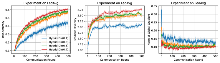
Figure 2: Observation: gradient diversity is related to convergence quality.

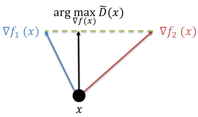
Figure 3: Solution of (7)

3.3 Mitigating Hybrid Heterogeneity Impacts

We conclude that a global update direction such that the maximum gradient diversity tends to efficiently mitigate hybrid heterogeneity. This direction is expected to significantly improve the federated optimization process, especially when dealing with hybrid heterogeneity.

Empirical observation on gradient diversity. To investigate the correlation between gradient diversity and convergence quality, we conduct an empirical study of FedAvg on partitioned CIFAR10 datasets, where the heterogeneous settings of Hybrid are described in Section 5. We partition the dataset with Dirichlet distribution with hyperparameters {0.1, 0.3, 0.5, 0.7}. We observe the training dynamics of test accuracy, gradient diversity, and global first-order gradient, as shown in Figure 3. We observe that curves corresponding to higher accuracy tend to converge to points with higher gradient diversity. This observation aligns with our previous analysis, where a larger value of gradient diversity indicates a lower global first-order gradient according to Corollary 3.1. This implies a reduced local drift by Corollary 3.2, and better performance. The observation reveals a positive relationship between gradient diversity and optimization quality.

This leads us to further examine the underlying meaning of a stationary point and its gradient diversity, which is related to the global first-order gradient. Considering the global objective is determined by weights $\lambda$, it raises the question of what are the best weights to reduce the impacts of statistical and system heterogeneity? By addressing this question, we can gain insights into designing effective global updates that mitigate heterogeneity and improve optimization performance. To this end, we use an adjustable $\tilde{\lambda}$ to study a surrogate global objective:

$$\tilde{f}(\boldsymbol{x})=\sum_{i=1}^{N}\tilde{\lambda}_{i}f_{i}(\boldsymbol{x}).$$

Correspondingly, we replace the global gradient in gradient diversity (3) regarding the surrogate objective:

Definition 3.2 (Surrogate gradient diversity).

We define the surrogate gradient diversity as the following ratio:

$$\tilde{D}(\boldsymbol{x}):=\sqrt{\frac{\sum_{i=1}^{N}\lambda_{i}\|\nabla f_{i}(\boldsymbol{x})\|^{2}}{\|\nabla\tilde{f}(\boldsymbol{x})\|^{2}}}\geq 1,$$ (6)

where $\nabla\tilde{f}(\boldsymbol{x})=\sum_{i=1}^{N}\tilde{\lambda}_{i}\nabla f_{i}(\boldsymbol{x})$ is the surrogate global gradient and remain the original $\lambda$ for local gradients.

In vanilla federated optimization, the global objective is deterministic for a fixed $\lambda$ (McMahan et al., 2017; Reddi et al., 2020; Wang et al., 2020). However, in our approach, we aim to design appropriate weights $\tilde{\lambda}$ that mitigate the impacts of hybrid heterogeneity and improve model performance. Based on our prior observation, maximizing gradient diversity can be a powerful metric for achieving this goal. The scheme aligns with previous studies leveraging $\lambda$ for FedAvg to improve the fairness (Li et al., 2019; Mohri et al., 2019), robustness (Li et al., 2020a).

Case study on gradient diversity maximization. To better illustrate this concept, we consider an FL system with two clients, where the gradient diversity is computed as follows:

$$\tilde{D}(x)=\sqrt{\frac{\lambda_{1}\|\nabla f_{1}(\boldsymbol{x})\|^{2}+\lambda_{2}\|\nabla f_{2}(\boldsymbol{x})\|^{2}}{\|\tilde{\lambda}_{1}\nabla f_{1}(\boldsymbol{x})+\tilde{\lambda}_{2}\nabla f_{2}(\boldsymbol{x})\|^{2}}}.$$ (7)

We note that the server cannot access local data samples. For each round, it only observes the local updates uploaded from clients. Hence, given a fixed point $x$, maximizing gradient diversity at the server is equivalent to minimizing the denominator of Equation 6. As a result, a global gradient direction that maximizes the gradient diversity leads to the solution in Figure 3.

For a general case where $N\geq 2$, given $x^{t}\in\mathbb{R}^{d}$, the local updates $\nabla f(\boldsymbol{x^{t}})$ are deterministic to the FL server. Maximizing the gradient diversity is minimizing the norm of weighted averaged global gradients $\|\nabla f(\boldsymbol{x})\|$. Therefore, our objective becomes:

$$\tilde{\lambda}=\min_{\lambda}\left\|\sum_{i=1}^{N}\lambda_{i}\nabla f_{i}(\boldsymbol{x})\right\|^{2},$$ (8)

which is subjected to $\sum_{i=1}^{N}\lambda_{i}=1,\lambda_{i}\geq 0\;\forall i$. The constrained optimization problem in (8) is to find a minimum-norm point in the convex hull of the set of input points. As the dimension of gradients can be millions, we use the Frank-Wolfe algorithm (Jaggi, 2013) to solve it. This procedure shares a similar sub-problem with multi-objective optimization works (Jaggi, 2013; Sener & Koltun, 2018; Zhou et al., 2022a), as we discussed in the next section. Furthermore, combining our previous analysis and observation in Figure 3, updating the global model towards the direction with maximized gradient diversity can alleviate statistical and system heterogeneity and improve optimization quality.

Main idea. In an FL system where clients are black-boxes to the server, it can be hard to find a static weight $\lambda$ to define the global objective that results in a stationary point with high testing accuracy. Gradient diversity maximization builds client weight for any feasible point $\boldsymbol{x}$, enabling the implementation of an adaptive surrogate global objective. Correspondingly, it creates an informative global update direction that mitigates hybrid heterogeneity impacts.

Algorithm 1 FedAWARE

0:  $\boldsymbol{x}^{0},\boldsymbol{m}^{0},\alpha$

1:  for round $t$ $\in$ $[T]$ do

2:     Server sample clients $S^{t}$ and broadcast model $\boldsymbol{x}^{t}$

3:     for client $i$ $\in$ $S^{t}$ in parallel do

4:        $\boldsymbol{x}^{t,0}_{i}=\boldsymbol{x}^{t}$

5:        for local update step $k$ $\in$ $[K_{i}]$ do

6:           $\boldsymbol{x}^{t,k}_{i}=\boldsymbol{x}^{t,k-1}_{i}-\eta_{l}\nabla F_{i}(\boldsymbol{x}^{t,k-1}_{i})$

7:        end for

8:        Client uploads local updates $\boldsymbol{g}_{i}^{t}=x^{t,0}-x^{t,K_{i}}$

9:     end for

10:     Server updates local momentum $\boldsymbol{m}_{i}^{t}=\begin{cases}\alpha\boldsymbol{m}_{i}^{t-1}+(1-\alpha)\boldsymbol{g}_{i}^{t},&\text{if}\;i\in S^{t}\\ \boldsymbol{m}_{i}^{t-1},&\text{if}\;i\notin S^{t}\end{cases}$

11:     Server computes $\tilde{\lambda}^{t}$ by (8) with $\boldsymbol{m}^{t}$

12:     Server computes global estimates $\boldsymbol{d}^{t}=\sum_{i=i}^{N}\tilde{\lambda}_{i}^{t}\boldsymbol{m}_{i}^{t}$ and updates $\boldsymbol{x}^{t+1}=\boldsymbol{x}^{t}-\eta\boldsymbol{d}^{t}$

13:  end for

4 Methodology of FedAWARE

In this section, we present a novel server-side optimizer FedAWARE, which addresses the challenges of hybrid heterogeneity without requiring local computing manipulation. We provide convergence analysis, with theoretical proof supplied in the Appendix. The pseudo-code for FedAWARE is provided in Algorithm 1.

Solving Equation 8 typically requires access to all local first-order gradients from clients, which is often infeasible in FL systems. To overcome this limitation, FedAWARE approximates utilizes the local updates using the history momentum of clients, denoted as $\boldsymbol{m}_{i},i\in[N]$. The update rule of momentum is controlled by a constant $\alpha$ in Line 10, Algorithm 1.

4.1 Convergence Analysis

We use local momentum to approximate the local updates. Besides, the local momentum can mitigate the unbalanced local drift. We provide the Lemma 4.1 to theoretically demonstrate the upper bound of the momentum approximation, which highlights that the momentum approximation can mitigate the hybrid heterogeneity with a proper setting of $\beta$. In this paper, we set $\alpha$ and $p$ to be the same for all clients. Our detailed analyses in the Appendix show the FedAWARE can be further improved by designing $\alpha$ and $p$ for each client, which we will study in future work.

Lemma 4.1.

Under Assumption 2.1 2.2 3.1, for any $i\in[N]$ and $t\in[T]$, the gap between momentum $\boldsymbol{m}_{i}$ and gradient $\nabla f_{i}(\boldsymbol{x}^{t})$ can be bounded:

$$\sum_{i=1}^{N}\lambda_{i}\mathbb{E}\left[\left\|\boldsymbol{m}_{i}^{t}-\nabla f_{i}(\boldsymbol{x}^{t})\right\|^{2}\right]\leq\beta^{2}L^{2}\underbrace{\sum_{i=1}^{N}\lambda_{i}\mathbb{E}{\left\|\boldsymbol{x}_{i}^{t,K_{i}}-\boldsymbol{x}^{t}\right\|^{2}}}_{\text{RHS of}~{}\eqref{eq:unbalanced_local_drift}}.$$

where we denote $\beta=(1-\alpha)p$ as a constant $p=p_{1}\cdots=p_{N}$, and $p_{i}=\text{Prob}(i\in S^{t})$.

Then, we present the convergence guarantee of Algorithm 1:

Theorem 4.1 (Convergence to the stationary points of Algorithm 1).

Under Assumption 2.1 2.2 3.1, following Lemma 4.1, the convergence of Algorithm 1 respecting arbitrary $\lambda$ can be bound

$$\min_{t\in[T]}\mathbb{E}\left[\left\|\nabla f(\boldsymbol{x}^{t})\right\|^{2}\right]\leq\epsilon_{\text{opt}}$$ (9)

$$\quad+\sum_{t=0}^{T-1}\frac{\beta L\tilde{G}\sqrt{\chi_{\tilde{\lambda}\|\lambda}^{2}}}{T\rho^{t}\tilde{D}(\boldsymbol{x}^{t})}\sqrt{\sigma^{2}+\Phi_{\text{Hetero}}},$$

where we denote $\sigma^{2}=5\eta_{l}(\sigma_{l}^{2}+6K_{\text{min}}^{2}\sigma_{g}^{2})$, $\chi_{\tilde{\lambda}\|\lambda}^{2}=\sum_{i=1}^{N}\frac{(\tilde{\lambda}_{i}^{t})^{2}}{\lambda_{i}^{2}}$, $\tilde{G}=\max_{t\in[T]}\sqrt{\sum_{i=1}^{N}\lambda_{i}\|\nabla f_{i}(\boldsymbol{x}^{t})\|^{2}}$. Besides, $\rho^{t}>0$ is an coefficient detailed in Appendix. The varnishing terms are hidden in $\epsilon_{\text{opt}}$.

We further provide the convergence related between the surrogate objective $\tilde{f}(\boldsymbol{x})$ and the original objective below.

Theorem 4.2 (Convergence of surrogate objective).

Under Assumptions 3.1, we have

$$\quad\min_{t\in[T]}\|\nabla\tilde{f}(\boldsymbol{x}^{t})\|^{2}\leq 2(N+\chi_{\tilde{\lambda}\|\lambda}^{2}-2\chi_{\tilde{\lambda}\|\lambda})\sigma_{g}^{2}$$

$$+2(1+N+\chi_{\tilde{\lambda}\|\lambda}^{2}-2\chi_{\tilde{\lambda}\|\lambda})\underbrace{\frac{1}{T}\sum_{t=0}^{T-1}\left\|\nabla f(\boldsymbol{x}^{t})\right\|^{2}}_{\text{RHS of}~{}\eqref{eq:final_rate}}.$$

Interpretation of convergence analysis. The terms $\sqrt{\sigma^{2}+\Phi_{\text{Hetero}}}$ reflect the impact of hybrid heterogeneity on the convergence rate. In other words, a large hybrid heterogeneity increases the convergence error, resulting in worse optimization performance. This paper evaluates the feasibility of updating the global model along with the gradient diversity maximization direction. Concretely, Algorithm 1 minimizes a surrogate global objective given by $\tilde{\lambda}$, while using term $\chi$ and Theorem 4.2 to denote the difference between the surrogate objective and the original objective. Specially, the surrogate objective (1) is dynamically determined by the $\tilde{\lambda}$ in Algorithm 1. Hence, the convergence rate denotes the status of the final stationary point and the speed of reaching it. It suggests that Algorithm 1 tends to make model $x$ converge to a point with large gradient diversity.

4.2 Discussion

To the best of our knowledge, this work is the first to consider gradient diversity as a positive factor in the convergence analysis. To clarify these differences, we provide additional discussion in the section.

Connection with multi-objective optimization (MOO). We note that Equation (8) is relevant to a sub-problem from MOO literature (Sener & Koltun, 2018; Hu et al., 2022; Zhou et al., 2022b). However, Algorithm 1 presents a federated optimization algorithm differently. Specifically, FedAWARE violates the basic Pareto partial order restriction in MOO. Besides, FedAWARE meets basic protocols in FL, including partial client participation and decoupled server/client optimization procedure, while MOO requires full participation and local first-order gradients in the FL context. In the FL literature, FedMGDA+ (Hu et al., 2022) also involves Equation (8) into federated optimization, but with a focus on FL fairness rather than heterogeneity. We found it cannot against hybrid heterogeneity issues studied in this paper as shown in Appendix, Figure 7.

Novelty in tackling heterogeneity. FedAWARE addresses hybrid heterogeneity by adjusting the denominator factor $\tilde{D}(\boldsymbol{x}^{t})$ in Theorem 4.1. In contrast, previous works are reducing the numerator terms corresponding with Theorem 4.1, which captures the impacts of hybrid heterogeneity. As discussed in Section 3.2, previous works minimize the upper bound of (5) to improve optimization quality. These works typically reduce the hybrid heterogeneity impacts by manipulating the local computation process. FedAWARE innovatively captures the gradient diversity trends and utilizes it to design global updates without manipulating local updates. This approach provides a novel perspective on addressing heterogeneity issues in FL.

Gradient diversity value. In our analysis, we first demonstrate that the upper bound of gradient diversity can be a positive factor in the convergence analysis. However, it is important to note that gradient diversity is not the sole factor for mitigating the impacts of heterogeneity. According to the convergence result in Theorem 4.1, the upper bound is determined by multiple factors, where gradient diversity is one feasible factor to minimize the upper bound. Furthermore, we have established a connection between gradient diversity and common assumptions on statistical heterogeneity in Section 3.1. It is worth mentioning that previous works (Li et al., 2020c; Karimireddy et al., 2020; Wang et al., 2020) take the upper bound of gradient diversity as a negative factor in the convergence analysis. Therefore, while they address heterogeneity issues in different ways, they ignore the evolution of gradient diversity.

Novelty in convergence analyses. The convergence analysis of FedAWARE introduces novel elements compared to previous federated optimization algorithms. While previous algorithms, such as FedAvg (McMahan et al., 2017), FedProx (Li et al., 2020c), and FedYogi (Reddi et al., 2020), assume a static global objective with uniform weights, FedAWARE analyzes the convergence of a surrogate objective with weights $\tilde{\lambda}$ based on stored momentum information. To differentiate from traditional federated optimization objectives, we use the term $\chi$ to highlight the differences. Furthermore, since FedAWARE does not manipulate the local computation process, we focus on the unbalanced local update steps, which absorb factors such as local training batch size, epochs, and local datasets. This approach allows us to address the concerns raised by FedNova (Wang et al., 2020) regarding objective inconsistency.

Limitations. The main limitation is that running Algorithm 1 requires the server to store the local momentum, which can be memory-intensive and may pose challenges for some resource-constrained devices or systems. Additional engineering optimizations may be needed in practice to address these limitations.

5 Experiments

We evaluate our theoretical findings and proposed algorithms in classic heterogeneous federated settings and show the hybrid heterogeneity damaging federated optimization algorithms. We empirically demonstrate how FedAWARE improves federated optimization. The experiment implementations are supported by FedLab (Zeng et al., 2023b).

Experimental setup. We compare federated optimization algorithms that roughly follow the Figure 1, including FedAvg (McMahan et al., 2017), FedAvgM (Hsu et al., 2019), FedProx (Li et al., 2020c), SCAFFOLD (Karimireddy et al., 2020), FedNova (Wang et al., 2020), FedYogi (Reddi et al., 2020) and FedDyn (Acar et al., 2020). Due to page limitation, we only report the results of training a CNN network on the CIFAR-10 dataset (Krizhevsky et al., 2009) in the main paper and evaluate the performance of the trained global model on the original CIFAR-10 test set. In the Appendix, we provide additional experiments on MNIST and FEMNIST. We also provide the hyper-parameters of baselines.

We construct three heterogeneous settings to evaluate our research: (1) Statistical Only: We adopt the identical Non-IID setup from FedAvg (McMahan et al., 2017). We sort the data that is sampled by labels, partition them into 200 blocks of equal size, and assign 100 clients with 2 blocks each. In this setting, we set a constant data batch size and local epoch for all clients, hence the number of local steps are balanced across clients. (2) Hybrid: We create federated datasets for 100 clients following the latent Dirichlet allocation over labels (Hsu et al., 2019). The hyper-parameter of the Dirichlet distribution is set to 0.1, indicating extreme statistical heterogeneity. In this setting, we also maintain a fixed data batch size and a local training epoch for all clients. The number of local steps differs amongst clients, resulting in system heterogeneity. (3) Hybrid+: Based on the hybrid setting described above, we dynamically set the local epoch $E_{i}\sim\mathcal{U}(2,5)$, and the batch size $B_{i}\sim\mathcal{U}(10,|\mathcal{D}_{i}|)$ for each round $t$ and selected client $i\in S^{t}$. Here, $\mathcal{U}$ denotes uniform distribution. Therefore, the local steps $K_{i}=\lfloor E_{i}*|\mathcal{D}_{i}|/B_{i}\rfloor$ are unstable. Each client conducts local mini-batch SGD with multiple local epochs to update the model.

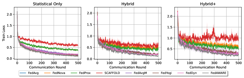
Figure 4: Test accuracy and train loss of federated optimization algorithms. we set the rate of client participation to be $10\%$, learning rate $\eta_{l}=0.01$, batch size $64$, and local epoch $3$ for all clients in the statistical-only and hybrid settings.

Figure 5: The evolution of gradient diversity versus communication rounds. FedAWARE converges to stationary points with higher gradient diversity than baselines.

Table 1: Top test accuracy (%$\pm$std)

Algorithms Heterogeneous Settings Statistical Only Hybrid Hybrid+ FedAvg 52.40$\pm$.47 50.47$\pm$.20 46.10$\pm$.19 FedAvgM 61.22$\pm$.23 58.13$\pm$.97 56.83$\pm$.73 FedProx 52.38$\pm$.51 50.58$\pm$.58 47.11$\pm$.38 SCAFFOLD 49.57$\pm$.08 50.61$\pm$.34 31.36$\pm$2.80 FedNova 52.39$\pm$.52 45.39$\pm$.32 40.98$\pm$1.50 FedYogi 61.07$\pm$1.51 59.10$\pm$.52 57.64$\pm$1.14 FedDyn 58.88$\pm$.41 56.85$\pm$.28 56.13$\pm$.41 FedAWARE 64.54$\pm$.38 61.41$\pm$.20 61.28$\pm$.39

Impacts of hybrid heterogeneity. In table 1, we detail the highest test accuracy. According to the top accuracy table, we observe that all federated optimization algorithms experience a deterioration in performance when transitioning from the statistical-only setting to the hybrid+ setting. This is because unbalanced local steps enlarge averaged local drifts, which aligns with Corollary 5. Hence, negatively affects optimization algorithms. Significantly, our algorithm maintains a superior performance, despite the heterogeneous challenges of varying degrees. In the experiments, we set $\alpha=0.5$. Moreover, we depict a sensitivity study about $\alpha$ on the hybrid+ setting in Appendix, Figure 7. The results show that FedAWARE could achieve better accuracy with a proper $\alpha$, which validates Lemma 4.1.

Convergence behavior of FedAWARE. We provide both the accuracy curve versus communication round in Figure 4 and the status of gradient diversity in Figure 5. According to the status curve of gradient diversity, FedAWARE converges to stationary points that preserve a higher gradient diversity. Moreover, observing the testing accuracy, we found that the curve of FedAWARE is more stable (less jitters and lower variance) than other baselines.

Gradient diversity observation. Regarding the status curve of gradient diversity, FedAWARE converges to stationary points that preserve a higher gradient diversity. In contrast, FedAvgM and FedYogi have lower gradient diversity while achieving a relatively high testing accuracy. This phenomenon matches our previous discussion that gradient diversity is not the only factor in convergence rate (9). Hence, high gradient diversity will not necessarily damage the federated optimization performance. In contrast, designing a better global update direction that maximizes gradient diversity can potentially achieve higher performance.

6 Conclusion

This paper emphasizes the importance of considering the effects of hybrid statistical and system heterogeneity challenges on federated optimization. We examine this issue through the lens of FL server optimization and conclude that pursuing gradient diversity maximization in the global update direction helps mitigate hybrid heterogeneity. Therefore, we propose server-side federated optimization methods that are applicable in scenarios exhibiting extreme hybrid heterogeneity and opaque clients. Our experimental evaluation demonstrates that our algorithm is robust to hybrid heterogeneity challenges and outperforms baseline federated optimization algorithms.

Appendix

The appendices are structured as follows:

• Appendix A: missed proofs in the main paper and useful lemmas.

• Appendix B: detailed convergence analysis of Algorithm 1.

• Appendix C: missed details about experimental hyperparameters and addition experiment results.

Appendix A Proof of Lemmas and Corollaries

Corollary A.1 (Bounded variance equivalence).

Let Assumption 3.1 hold. Then, in the case of bounded variance, i.e.,$\sum_{i=1}^{N}\lambda_{i}\left\|\nabla f_{i}(\boldsymbol{x})-\nabla f(\boldsymbol{x})\right\|^{2}\leq\sigma_{g}^{2}$, it follows that $D(\boldsymbol{x})\leq\sqrt{1+\frac{\sigma_{g}^{2}}{\|\nabla f(\boldsymbol{x})\|^{2}}}$.

Proof.

$$\sum_{i=1}^{N}\lambda_{i}\left\|\nabla f_{i}(\boldsymbol{x})-\nabla f(\boldsymbol{x})\right\|^{2}\leq\sum_{i=1}^{N}\lambda_{i}\left\|\nabla f_{i}(\boldsymbol{x})\right\|^{2}-\|\nabla f(\boldsymbol{x})\|^{2}\leq\sigma_{g}^{2}$$

$$\Leftrightarrow \sum_{i=1}^{N}\lambda_{i}\left\|\nabla f_{i}(\boldsymbol{x})\right\|^{2}\leq\sigma_{g}^{2}+\|\nabla f(\boldsymbol{x})\|^{2}$$

$$\Rightarrow D(\boldsymbol{x})=\sqrt{\frac{\sum_{i=1}^{N}\lambda_{i}\|\nabla f_{i}(\boldsymbol{x})\|^{2}}{\|\nabla f(\boldsymbol{x})\|^{2}}}\leq\sqrt{\frac{\sigma_{g}^{2}+\|\nabla f(\boldsymbol{x})\|^{2}}{\|\nabla f(\boldsymbol{x})\|^{2}}}\leq\sqrt{1+\frac{\sigma_{g}^{2}}{\|\nabla f(\boldsymbol{x})\|^{2}}}.$$

∎

Lemma A.1 (Modified upper bound of local drift, Reddi et al., 2020).

Let Assumption 2.2 3.1 hold. For all client $i\in[N]$ with arbitrary local iteration steps $k\in[K_{i}]$, the local drift can be bounded as follows,

$$\mathbb{E}\left\|\boldsymbol{x}_{i}^{t,k}-\boldsymbol{x}^{t}\right\|^{2}\leq 5K_{i}\eta_{l}^{2}(\sigma_{l}^{2}+6K_{i}\zeta_{i}(\boldsymbol{x}^{t})+6K_{i}\left\|\nabla f\left(\boldsymbol{x}^{t}\right)\right\|^{2}).$$

Proof.

For $k\in[K_{i}]$, we have

$$\quad\mathbb{E}\left[\left\|\boldsymbol{g}_{i}^{t}\right\|^{2}\right]=\mathbb{E}\left\|\boldsymbol{x}_{i}^{t,k}-\boldsymbol{x}^{t}\right\|^{2}=\mathbb{E}\left\|\boldsymbol{x}_{i}^{t,k-1}-\boldsymbol{x}^{t}-\eta_{l}\nabla F_{i}(\boldsymbol{x}_{i}^{t,k-1})\right\|^{2}$$

$$= \mathbb{E}\left\|\boldsymbol{x}_{i}^{t,k-1}-\boldsymbol{x}^{t}-\eta_{l}(\nabla F_{i}(\boldsymbol{x}_{i}^{t,k-1})\pm\nabla f_{i}(\boldsymbol{x}_{i}^{t,k-1}))\right\|^{2}$$

$$= \mathbb{E}\left\|\boldsymbol{x}_{i}^{t,k-1}-\boldsymbol{x}^{t}-\eta_{l}\nabla f_{i}(\boldsymbol{x}_{i}^{t,k-1}))\right\|^{2}+\mathbb{E}\left\|\eta_{l}\left(\nabla F_{i}(\boldsymbol{x}_{i}^{t,k-1})-\nabla f_{i}\left(\boldsymbol{x}_{i}^{t,k-1}\right)\right)\right\|^{2}$$

$$= \mathbb{E}\left[\left\|\boldsymbol{x}_{i}^{t,k-1}-\boldsymbol{x}^{t}\right\|^{2}-2<\boldsymbol{x}_{i}^{t,k-1}-\boldsymbol{x}^{t},\eta_{l}\nabla f_{i}(\boldsymbol{x}_{i}^{t,k-1})>+\left\|\eta_{l}\nabla f_{i}(\boldsymbol{x}_{i}^{t,k-1})\right\|^{2}\right]+\eta_{l}^{2}\sigma_{l}^{2}$$

$$= \mathbb{E}\left[\left\|\boldsymbol{x}_{i}^{t,k-1}-\boldsymbol{x}^{t}\right\|^{2}-2<\frac{1}{\sqrt{2K_{i}-1}}(\boldsymbol{x}_{i}^{t,k-1}-\boldsymbol{x}^{t}),\sqrt{2K_{i}-1}\eta_{l}\nabla f_{i}(\boldsymbol{x}_{i}^{t,k-1})>+\left\|\eta_{l}\nabla f_{i}(\boldsymbol{x}_{i}^{t,k-1})\right\|^{2}\right]+\eta_{l}^{2}\sigma_{l}^{2}$$

$$\leq \left(1+\frac{1}{2K_{i}-1}\right)\mathbb{E}\left[\left\|\boldsymbol{x}_{i}^{t,k-1}-\boldsymbol{x}^{t}\right\|^{2}\right]+2K_{i}\mathbb{E}\left[\left\|\eta_{l}\nabla f_{i}(\boldsymbol{x}_{i}^{t,k-1})\right\|^{2}\right]+\eta_{l}^{2}\sigma_{l}^{2}$$

$$= \left(1+\frac{1}{2K_{i}-1}\right)\mathbb{E}\left[\left\|\boldsymbol{x}_{i}^{t,k-1}-\boldsymbol{x}^{t}\right\|^{2}\right]+2K_{i}\mathbb{E}\left[\left\|\eta_{l}\left(\nabla f_{i}(\boldsymbol{x}_{i}^{t,k-1})\pm\nabla f\left(\boldsymbol{x}^{t}\right)\pm\nabla f_{i}\left(\boldsymbol{x}^{t}\right)\right)\right\|^{2}\right]+\eta_{l}^{2}\sigma_{l}^{2}$$

$$\leq \left(1+\frac{1}{2K_{i}-1}\right)\mathbb{E}\left\|\boldsymbol{x}_{i}^{t,k-1}-\boldsymbol{x}^{t}\right\|^{2}+6K_{i}\mathbb{E}\left[\left\|\eta_{l}\left(\nabla f_{i}\left(\boldsymbol{x}_{i}^{t,k-1}\right)-\nabla f_{i}\left(\boldsymbol{x}^{t}\right)\right)\right\|^{2}\right]+6K_{i}\mathbb{E}\left[\left\|\eta_{l}\left(\nabla f_{i}\left(\boldsymbol{x}^{t}\right)\right)\right\|^{2}\right]+\eta_{l}^{2}\sigma_{l}^{2}$$

$$\leq \left(1+\frac{1}{2K_{i}-1}+6K_{i}\eta_{l}^{2}L^{2}\right)\mathbb{E}\left\|\boldsymbol{x}_{i}^{t,k-1}-\boldsymbol{x}^{t}\right\|^{2}+\eta_{l}^{2}(\sigma_{l}^{2}+6K_{i}\zeta_{i}(\boldsymbol{x}^{t})+6K_{i}\mathbb{E}\left[\left\|\nabla f\left(\boldsymbol{x}^{t}\right)\right\|^{2}\right])$$

Unrolling the recursion, we obtain

$$\mathbb{E}\left\|\boldsymbol{x}_{i}^{t,k}-\boldsymbol{x}^{t}\right\|^{2}\leq \sum_{p=0}^{k-1}\left(1+\frac{1}{2K_{i}-1}+4K_{i}\eta_{l}^{2}L^{2}\right)^{p}\eta_{l}^{2}(\sigma_{l}^{2}+6K_{i}\zeta_{i}(\boldsymbol{x}^{t})+6K_{i}\mathbb{E}\left[\left\|\nabla f\left(\boldsymbol{x}^{t}\right)\right\|^{2}\right])$$ (10)

$$\leq (K_{i}-1)\left[\left(1+\frac{1}{K_{i}-1}\right)^{K_{i}}-1\right]\eta_{l}^{2}(\sigma_{l}^{2}+6K_{i}\zeta_{i}(\boldsymbol{x}^{t})+6K_{i}\mathbb{E}\left[\left\|\nabla f\left(\boldsymbol{x}^{t}\right)\right\|^{2}\right])$$

$$\leq 5K_{i}\eta_{l}^{2}(\sigma_{l}^{2}+6K_{i}\zeta_{i}(\boldsymbol{x}^{t})+6K_{i}\mathbb{E}\left\|\nabla f\left(\boldsymbol{x}^{t}\right)\right\|^{2})$$

where we use the fact that $(1+\frac{1}{K_{i}-1})^{K_{i}}\leq 5$ for $K_{i}>1$. ∎

Lemma A.2 (Upper bound of balanced local drift).

Let Assumption 2.2 3.1 hold. For any client $i\in[N]$ with arbitrary local iteration steps $k\in[K]$ with local learning rate $\eta_{l}\leq\frac{1}{K}$, the average of local drift can be bounded as follows,

$$\mathbb{E}\left\|\sum_{i=1}^{N}\lambda_{i}\boldsymbol{x}_{i}^{t,k}-\boldsymbol{x}^{t}\right\|^{2}\leq\sum_{i=1}^{N}\lambda_{i}\mathbb{E}\left\|\boldsymbol{x}_{i}^{t,k}-\boldsymbol{x}^{t}\right\|^{2}\leq 5\eta_{l}(\sigma_{l}^{2}+6K\sigma_{g}^{2}+6K\mathbb{E}\left\|\nabla f\left(\boldsymbol{x}^{t}\right)\right\|^{2})$$ (11)

Corollary A.2 (Loose upper bound of unbalanced local drift).

Let Assumption 2.2 3.1 hold. For any client $i\in[N]$ with arbitrary local iteration steps $k\in[K_{i}]$ with local learning rate $\eta_{l}\leq\frac{1}{K_{i}}$, the average of local drift can be bounded as follows,

$$\mathbb{E}\left\|\sum_{i=1}^{N}\lambda_{i}\boldsymbol{x}_{i}^{t,k}-\boldsymbol{x}^{t}\right\|^{2} \leq\sum_{i=1}^{N}\lambda_{i}\mathbb{E}\left\|\boldsymbol{x}_{i}^{t,k}-\boldsymbol{x}^{t}\right\|^{2}\leq 5\eta_{l}(\sigma_{l}^{2}+6K_{\text{min}}^{2}\sigma_{g}^{2}+6\tilde{K}\mathbb{E}\left\|\nabla f\left(\boldsymbol{x}^{t}\right)\right\|^{2})+\Phi_{\text{Hetero}},$$ (12)

where $\tilde{K}=\sum_{i=1}^{N}\lambda_{i}K_{i}$, $\Phi_{\text{Hetero}}=\sum_{i=1}^{N}30\eta_{l}(K_{i}-K_{\text{min}})\zeta_{i}(\boldsymbol{x}^{t}).$

Appendix B Convergence Analysis

This section provides detailed proof of Theorem 4.1. Our theory examines the impacts of gradient diversity in federated optimization and matches the convergence of classic aggregation-based methods, such as FedAvg. The Algorithm 1 manipulates the aggregation results with momentum approximation and adaptive weight strategies in a different manner with FedAvg.

Proof.

We recall the updated rule of Algorithm 1 is:

$$\boldsymbol{x}^{t+1}=\boldsymbol{x}^{t}-\eta\boldsymbol{d}^{t},$$

where

$$\boldsymbol{d}^{t}=\sum_{i=1}^{N}\tilde{\lambda}^{t}_{i}\boldsymbol{m}_{i}^{t},\text{s.t.}\;\tilde{\lambda}^{t}=\underset{\lambda}{\arg\min}\left\|\sum_{i=1}^{N}\lambda_{i}\boldsymbol{m}_{i}^{t}\right\|^{2}.$$

Using the smoothness, we have:

$$f\left(\boldsymbol{x}^{t+1}\right) =f\left(\boldsymbol{x}^{t}-\eta\boldsymbol{d}^{t}\right)\leq f\left(\boldsymbol{x}^{t}\right)-\eta\left\langle\nabla f\left(\boldsymbol{x}^{t}\right),\boldsymbol{d}^{t}\right\rangle+\frac{L}{2}\eta^{2}\left\|\boldsymbol{d}^{t}\right\|^{2}$$

$$\leq f\left(\boldsymbol{x}^{t}\right)-\eta\left\langle\nabla f\left(\boldsymbol{x}^{t}\right),\boldsymbol{d}^{t}-\nabla f\left(\boldsymbol{x}^{t}\right)+\nabla f\left(\boldsymbol{x}^{t}\right)\right\rangle+\frac{L}{2}\eta^{2}\left\|\boldsymbol{d}^{t}\right\|^{2}$$

$$\leq f\left(\boldsymbol{x}^{t}\right)-\eta\|\nabla f\left(\boldsymbol{x}^{t}\right)\|^{2}+\eta\left\langle\nabla f\left(\boldsymbol{x}^{t}\right),\nabla f\left(\boldsymbol{x}^{t}\right)-\boldsymbol{d}^{t}\right\rangle+\frac{L}{2}\eta^{2}\left\|\boldsymbol{d}^{t}\right\|^{2}.$$

Taking full expectation over randomness at time step $t$ on both sides, we have:

$$\mathbb{E}\left[f(\boldsymbol{x}^{t+1})\right]-f(\boldsymbol{x}^{t}) \leq-\eta\mathbb{E}\|\nabla f\left(\boldsymbol{x}^{t}\right)\|^{2}+\eta\underbrace{\mathbb{E}[\langle\nabla f(\boldsymbol{x}^{t}),\nabla f\left(\boldsymbol{x}^{t}\right)-\boldsymbol{d}^{t}\rangle]}_{T_{1}}+\frac{L}{2}\eta^{2}\underbrace{\mathbb{E}[\|\boldsymbol{d}^{t}\|^{2}]}_{T_{2}}.$$ (13)

Now, we are about to bound $T_{1}$ and $T_{2}$ respectively.

Bounding $T_{1}$. By Cauchy-Schwartz inequality, we get

$$T_{1} \leq\mathbb{E}\left[\left\|\nabla f(\boldsymbol{x}^{t})\right\|\left\|\nabla f(\boldsymbol{x}^{t})-\boldsymbol{d}^{t}\right\|\right]\leq\mathbb{E}\left\|\nabla f(\boldsymbol{x}^{t})\right\|\mathbb{E}\left[\left\|\sum_{i=1}^{N}\lambda_{i}\nabla f_{i}(\boldsymbol{x}^{t})-\sum_{i=1}^{N}\tilde{\lambda}_{i}^{t}\boldsymbol{m}_{i}^{t}\right\|\right]$$

$$=\mathbb{E}\left\|\nabla f(\boldsymbol{x}^{t})\right\|\mathbb{E}\left[\left\|\sum_{i=1}^{N}\lambda_{i}\nabla f_{i}(\boldsymbol{x}^{t})\pm\sum_{i=1}^{N}\tilde{\lambda}_{i}f_{i}(\boldsymbol{x}^{t})-\sum_{i=1}^{N}\tilde{\lambda}_{i}^{t}\boldsymbol{m}_{i}^{t}\right\|\right]$$

$$\leq\mathbb{E}\left\|\nabla f(\boldsymbol{x}^{t})\right\|\mathbb{E}\left[\left\|\sum_{i=1}^{N}(\lambda_{i}-\tilde{\lambda}_{i}^{t})\nabla f_{i}(\boldsymbol{x}^{t})\right\|\right]+\mathbb{E}\left\|\nabla f(\boldsymbol{x}^{t})\right\|\mathbb{E}\left[\left\|\sum_{i=1}^{N}\tilde{\lambda}_{i}^{t}(\nabla f_{i}(\boldsymbol{x}^{t})-\boldsymbol{m}_{i}^{t})\right\|\right]$$

$$\leq\mathbb{E}\left\|\nabla f(\boldsymbol{x}^{t})\right\|\mathbb{E}\left[\left\|\sum_{i=1}^{N}\frac{(\lambda_{i}-\tilde{\lambda}_{i}^{t})}{\lambda_{i}}\cdot\lambda_{i}\nabla f_{i}(\boldsymbol{x}^{t})\right\|\right]+\mathbb{E}\left\|\nabla f(\boldsymbol{x}^{t})\right\|\mathbb{E}\left[\left\|\sum_{i=1}^{N}\frac{\tilde{\lambda}_{i}^{t}}{\lambda_{i}}\cdot\lambda_{i}(\nabla f_{i}(\boldsymbol{x}^{t})-\boldsymbol{m}_{i}^{t})\right\|\right]$$

$$\leq\sqrt{\sum_{i=1}^{N}\frac{(\lambda_{i}-\tilde{\lambda}_{i}^{t})^{2}}{\lambda_{i}^{2}}}\mathbb{E}\left\|\nabla f(\boldsymbol{x}^{t})\right\|\mathbb{E}\left[\left\|\sum_{i=1}^{N}\lambda_{i}\nabla f_{i}(\boldsymbol{x}^{t})\right\|\right]+\sqrt{\sum_{i=1}^{N}\frac{(\tilde{\lambda}_{i}^{t})^{2}}{\lambda_{i}^{2}}}\mathbb{E}\left\|\nabla f(\boldsymbol{x}^{t})\right\|\mathbb{E}\left[\left\|\sum_{i=1}^{N}\lambda_{i}(\nabla f_{i}(\boldsymbol{x}^{t})-\boldsymbol{m}_{i}^{t})\right\|\right]$$

$$\leq\sqrt{\sum_{i=1}^{N}\frac{(\lambda_{i}-\tilde{\lambda}_{i}^{t})^{2}}{\lambda_{i}^{2}}}\mathbb{E}\left\|\nabla f(\boldsymbol{x}^{t})\right\|^{2}+\sqrt{\sum_{i=1}^{N}\frac{(\tilde{\lambda}_{i}^{t})^{2}}{\lambda_{i}^{2}}}\mathbb{E}\left\|\nabla f(\boldsymbol{x}^{t})\right\|\mathbb{E}\left[\left\|\sum_{i=1}^{N}\lambda_{i}(\nabla f_{i}(\boldsymbol{x}^{t})-\boldsymbol{m}_{i}^{t})\right\|\right],$$

where we use Cauchy-Schwartz inequality to decompose the $\tilde{\lambda}$ from norms.

Then, using the fact that $\mathbb{E}^{2}\|A\|\leq\mathbb{E}\|A\|^{2}$, we have

$$T_{1} \leq\sqrt{\sum_{i=1}^{N}\frac{(\lambda_{i}-\tilde{\lambda}_{i}^{t})^{2}}{\lambda_{i}^{2}}}\mathbb{E}\left\|\nabla f(\boldsymbol{x}^{t})\right\|^{2}+\sqrt{\sum_{i=1}^{N}\frac{(\tilde{\lambda}_{i}^{t})^{2}}{\lambda_{i}^{2}}}\sqrt{\mathbb{E}\left[\left\|\sum_{i=1}^{N}\lambda_{i}(\nabla f_{i}(\boldsymbol{x}^{t})-\boldsymbol{m}_{i}^{t})\right\|^{2}\right]}\mathbb{E}\left\|\nabla f(\boldsymbol{x}^{t})\right\|$$

$$\leq\sqrt{\sum_{i=1}^{N}\frac{(\lambda_{i}-\tilde{\lambda}_{i}^{t})^{2}}{\lambda_{i}^{2}}}\mathbb{E}\left\|\nabla f(\boldsymbol{x}^{t})\right\|^{2}+\sqrt{\sum_{i=1}^{N}\frac{(\tilde{\lambda}_{i}^{t})^{2}}{\lambda_{i}^{2}}}\sqrt{\sum_{i=1}^{N}\lambda_{i}\mathbb{E}\left[\left\|\nabla f_{i}(\boldsymbol{x}^{t})-\boldsymbol{m}_{i}^{t}\right\|^{2}\right]}\mathbb{E}\left\|\nabla f(\boldsymbol{x}^{t})\right\|.$$

Letting $\chi_{\tilde{\lambda}\|\lambda}^{2}=\sum_{i=1}^{N}\frac{(\tilde{\lambda}_{i}^{t})^{2}}{\lambda_{i}^{2}},\chi_{\tilde{\lambda}\|\lambda}=\sum_{i=1}^{N}\frac{(\tilde{\lambda}_{i}^{t})}{\lambda_{i}}$, we have

$$T_{1}\leq\sqrt{1+\chi_{\tilde{\lambda}\|\lambda}^{2}-2\chi_{\tilde{\lambda}\|\lambda}}\mathbb{E}\left\|\nabla f(\boldsymbol{x}^{t})\right\|^{2}+\sqrt{\chi_{\tilde{\lambda}\|\lambda}^{2}}\sqrt{\sum_{i=1}^{N}\lambda_{i}\mathbb{E}\left[\left\|\nabla f_{i}(\boldsymbol{x}^{t})-\boldsymbol{m}_{i}^{t}\right\|^{2}\right]}\cdot\mathbb{E}\left\|\nabla f(\boldsymbol{x}^{t})\right\|.$$ (14)

Bounding $T_{2}$. By the definitions and triangle inequality, we can decompose the $T_{1}$,

$$T_{2} =\mathbb{E}[\|\boldsymbol{d}^{t}\|^{2}]=\mathbb{E}\left[\left\|\sum_{i=1}^{N}\tilde{\lambda}_{i}^{t}\boldsymbol{m}_{i}^{t}\right\|^{2}\right]=\mathbb{E}\left[\left\|\sum_{i=1}^{N}\tilde{\lambda}_{i}^{t}\boldsymbol{m}_{i}^{t}-\sum_{i=1}^{N}\tilde{\lambda}_{i}^{t}\nabla f_{i}(\boldsymbol{x}^{t})+\sum_{i=1}^{N}\tilde{\lambda}_{i}^{t}\nabla f_{i}(\boldsymbol{x}^{t})\right\|^{2}\right]$$ (15)

$$\leq 2\mathbb{E}\left[\left\|\sum_{i=1}^{N}\tilde{\lambda}_{i}^{t}(\boldsymbol{m}_{i}^{t}-\nabla f_{i}(\boldsymbol{x}^{t}))\right\|^{2}\right]+2\mathbb{E}\left[\left\|\sum_{i=1}^{N}(\tilde{\lambda}_{i}^{t}-\lambda_{i})\nabla f_{i}(\boldsymbol{x}^{t})\right\|^{2}\right]$$

$$\leq 2\mathbb{E}\left[\left\|\sum_{i=1}^{N}\frac{\tilde{\lambda}_{i}^{t}}{\lambda_{i}}\cdot\lambda_{i}(\boldsymbol{m}_{i}^{t}-\nabla f_{i}(\boldsymbol{x}^{t}))\right\|^{2}\right]+2\mathbb{E}\left[\left\|\sum_{i=1}^{N}\frac{(\tilde{\lambda}_{i}^{t}-\lambda_{i})}{\lambda_{i}}\cdot\lambda_{i}\nabla f_{i}(\boldsymbol{x}^{t})\right\|^{2}\right]$$

$$\leq 2\chi_{\tilde{\lambda}\|\lambda}^{2}\mathbb{E}\left[\left\|\sum_{i=1}^{N}\lambda_{i}(\boldsymbol{m}_{i}^{t}-\nabla f_{i}(\boldsymbol{x}^{t}))\right\|^{2}\right]+2(N+\chi_{\tilde{\lambda}\|\lambda}^{2}-2\chi_{\tilde{\lambda}\|\lambda})\mathbb{E}\left[\left\|\nabla f(\boldsymbol{x}^{t})\right\|^{2}\right]$$

$$\leq 2\chi_{\tilde{\lambda}\|\lambda}^{2}\sum_{i=1}^{N}\lambda_{i}\mathbb{E}\left[\left\|(\boldsymbol{m}_{i}^{t}-\nabla f_{i}(\boldsymbol{x}^{t}))\right\|^{2}\right]+2(N+\chi_{\tilde{\lambda}\|\lambda}^{2}-2\chi_{\tilde{\lambda}\|\lambda})\mathbb{E}\left[\left\|\nabla f(\boldsymbol{x}^{t})\right\|^{2}\right],$$

where we also use Cauchy-Schwartz inequality to decompose $\tilde{\lambda}$.

Investigating momentum approximation. Observing (14) and (15), we need to bound the approximation error of local momentum. We present our analysis in the following lemma.

Lemma B.1 (Bound of local momentum).

For any $i\in[N]$ and $t\in[T]$, letting $\beta_{i}=(1-\alpha)p_{i}\leq 1$ and $p_{i}=\text{Prob}(i\in S^{t})$, the gap between momentum $\boldsymbol{m}_{i}$ and gradient $\nabla f_{i}(\boldsymbol{x}^{t})$ can be bounded:

$$\sum_{i=1}^{N}\lambda_{i}\mathbb{E}\left[\left\|\boldsymbol{m}_{i}^{t}-\nabla f_{i}(\boldsymbol{x}^{t})\right\|^{2}\right]\leq\beta^{2}L^{2}\sum_{i=1}^{N}\lambda_{i}\mathbb{E}{\left\|\boldsymbol{x}_{i}^{t,K_{i}}-\boldsymbol{x}^{t}\right\|^{2}}.$$ (16)

Proof.

$$\quad\;\sum_{i=1}^{N}\lambda_{i}\mathbb{E}{\left[\left\|\boldsymbol{m}_{i}^{t}-\nabla f_{i}(\boldsymbol{x}^{t})\right\|^{2}\right]}$$

$$=\sum_{i=1}^{N}\lambda_{i}\mathbb{E}{\left[\left\|(1-p_{i})\boldsymbol{m}_{i}^{t-1}+p_{i}(\alpha\boldsymbol{m}_{i}^{t-1}+(1-\alpha)\boldsymbol{g}_{i}^{t})-\nabla f_{i}(\boldsymbol{x}^{t})\right\|^{2}\right]}$$

$$=\sum_{i=1}^{N}\lambda_{i}\mathbb{E}{\left[\left\|[1-(1-\alpha)p_{i}]\boldsymbol{m}_{i}^{t-1}+(1-\alpha)p_{i}\boldsymbol{g}_{i}^{t}-\nabla f_{i}(\boldsymbol{x}^{t})\right\|^{2}\right]}$$

$$=\sum_{i=1}^{N}\lambda_{i}\mathbb{E}{\left[\left\|(1-\beta_{i})\boldsymbol{m}_{i}^{t-1}+\beta_{i}\boldsymbol{g}_{i}^{t}-\nabla f_{i}(\boldsymbol{x}^{t})\right\|^{2}\right]}\quad\quad\quad\text{$\triangleright$ letting $\beta_{i}=(1-\alpha)p_{i}$}$$

$$=\sum_{i=1}^{N}\lambda_{i}\mathbb{E}{\left[\left\|(1-\beta_{i})(\boldsymbol{m}_{i}^{t-1}-\nabla f_{i}(\boldsymbol{x}^{t-1}))+\beta_{i}\boldsymbol{g}_{i}^{t}+(1-\beta_{i})\nabla f_{i}(\boldsymbol{x}^{t-1})-\nabla f_{i}(\boldsymbol{x}^{t})\right\|^{2}\right]}$$

$$=\sum_{i=1}^{N}\lambda_{i}\mathbb{E}{\left[\left\|(1-\beta_{i})(\boldsymbol{m}_{i}^{t-1}-\nabla f_{i}(\boldsymbol{x}^{t-1}))+\beta_{i}[\boldsymbol{g}_{i}^{t}-\eta_{l}K_{i}\nabla f_{i}(\boldsymbol{x}^{t})]+\left((1-\beta_{i})\nabla f_{i}(\boldsymbol{x}^{t-1})-(1-\beta_{i}\eta_{l}K_{i})\right)\nabla f_{i}(\boldsymbol{x}^{t})\right\|^{2}\right]}$$

$$\leq\sum_{i=1}^{N}\lambda_{i}(1-\beta_{i})^{2}\mathbb{E}{\left[\left\|\boldsymbol{m}_{i}^{t-1}-\nabla f_{i}(\boldsymbol{x}^{t-1})\right\|^{2}\right]}+\sum_{i=1}^{N}\lambda_{i}\beta_{i}^{2}\underbrace{\mathbb{E}\left[\left\|\boldsymbol{g}_{i}^{t}-\eta_{l}K_{i}\nabla f_{i}(\boldsymbol{x}^{t})\right\|^{2}\right]}_{R_{1}}+\sum_{i=1}^{N}\lambda_{i}(1-\beta_{i})^{2}L^{2}\underbrace{\mathbb{E}\left\|\boldsymbol{x}^{t-1}-\boldsymbol{x}^{t}\right\|^{2}}_{\mathbb{E}\|\eta\boldsymbol{d}^{t-1}\|^{2}}.$$

Note that the term $R_{1}$ denotes the heterogeneity brought by the local computation. For $\tau\in[t]$, term $R_{1}$ can be bounded,

$$R_{1} =\mathbb{E}{\left[\left\|\sum_{k=1}^{K_{i}}\eta_{l}\nabla F_{i}(\boldsymbol{x}^{t,k})-\eta_{l}K_{i}\nabla f_{i}(\boldsymbol{x}^{t})\right\|^{2}\right]}=\mathbb{E}{\left[\left\|\sum_{k=1}^{K_{i}}\eta_{l}\left(\nabla F_{i}(\boldsymbol{x}^{t,k})-\nabla f_{i}(\boldsymbol{x}^{t})\right)\right\|^{2}\right]}$$ (17)

$$=\mathbb{E}{\left[\left\|\sum_{k=1}^{K_{i}}\eta_{l}\left(\nabla f_{i}(\boldsymbol{x}^{t,k})-\nabla f_{i}(\boldsymbol{x}^{t})\right)\right\|^{2}\right]}\quad\quad\text{$\triangleright$ using Assumption~{}\ref{asp:unbiasedness}}$$

$$\leq L^{2}\eta_{l}^{2}\sum_{k=1}^{K_{i}}\mathbb{E}{\left\|\boldsymbol{x}_{i}^{t,k}-\boldsymbol{x}^{t}\right\|^{2}}\quad\quad\text{$\triangleright$ using Assumption~{}\ref{asp:smoothness}}$$

$$\leq L^{2}\eta_{l}^{2}K_{i}\mathbb{E}{\left\|\boldsymbol{x}_{i}^{t,K_{i}}-\boldsymbol{x}^{t}\right\|^{2}}.$$

And, using (15) to bound the second term, we have

$$\mathbb{E}\|\eta\boldsymbol{d}^{t-1}\|^{2} =\eta^{2}\mathbb{E}\|\boldsymbol{d}^{t-1}\|^{2}$$ (18)

$$\leq 2\eta^{2}\chi_{\tilde{\lambda}\|\lambda}^{2}\sum_{i=1}^{N}\lambda_{i}\mathbb{E}\left[\left\|(\boldsymbol{m}_{i}^{t}-\nabla f_{i}(\boldsymbol{x}^{t-1}))\right\|^{2}\right]+2\eta^{2}(N+\chi_{\tilde{\lambda}\|\lambda}^{2}-2\chi_{\tilde{\lambda}\|\lambda})\mathbb{E}\left[\left\|\nabla f(\boldsymbol{x}^{t-1})\right\|^{2}\right]$$

Combining the equations, we have

$$\sum_{i=1}^{N}\lambda_{i}\mathbb{E}{\left[\left\|\boldsymbol{m}_{i}^{t}-\nabla f_{i}(\boldsymbol{x}^{t})\right\|^{2}\right]}$$ (19)

$$\leq \sum_{i=1}^{N}\lambda_{i}(1-\beta_{i})^{2}(1+2L^{2}\eta^{2}\chi_{\tilde{\lambda}\|\lambda}^{2})\mathbb{E}{\left[\left\|\boldsymbol{m}_{i}^{t-1}-\nabla f_{i}(\boldsymbol{x}^{t-1})\right\|^{2}\right]}+\sum_{i=1}^{N}\lambda_{i}\beta_{i}^{2}L^{2}\eta_{l}^{2}K_{i}\mathbb{E}{\left\|\boldsymbol{x}_{i}^{t,K_{i}}-\boldsymbol{x}^{t}\right\|^{2}}$$

$$\quad+\left[\sum_{i=1}^{N}\lambda_{i}(1-\beta_{i})^{2}\right]2L^{2}\eta^{2}(N+\chi_{\tilde{\lambda}\|\lambda}^{2}-2\chi_{\tilde{\lambda}\|\lambda})\cdot\left\|\nabla f(\boldsymbol{x}^{t-1})\right\|^{2}.$$

As the last term of (19) typically vanishes over time $T$ due to factors $\beta$ and $\eta$, we omit the last term and mainly focus on the effects of the second term. Unrolling the recursion for $i\in[N]$, we have

$$\sum_{i=1}^{N}\lambda_{i}\mathbb{E}\left[\left\|\boldsymbol{m}_{i}^{t}-\nabla f_{i}(\boldsymbol{x}^{t})\right\|^{2}\right]$$ (20)

$$\leq \sum_{i=1}^{N}\lambda_{i}\sum_{\tau=1}^{t}\left((1-\beta_{i})^{2}(1+2L^{2}\eta^{2}\chi_{\tilde{\lambda}\|\lambda}^{2})\right)^{\tau-1}\beta_{i}^{2}L^{2}\eta_{l}^{2}K_{i}\mathbb{E}{\left\|\boldsymbol{x}_{i}^{t,K_{i}}-\boldsymbol{x}^{t}\right\|^{2}}$$

$$\leq \sum_{i=1}^{N}\lambda_{i}t\max_{\tau\in[t]}\left((1-\beta_{i})^{2}(1+2L^{2}\eta^{2}\chi_{\tilde{\lambda}\|\lambda}^{2})\right)^{\tau-1}\beta_{i}^{2}L^{2}\eta_{l}^{2}K_{i}\mathbb{E}{\left\|\boldsymbol{x}_{i}^{t,K_{i}}-\boldsymbol{x}^{t}\right\|^{2}}$$

$$\leq \sum_{i=1}^{N}\lambda_{i}t\beta_{i}^{2}L^{2}\eta_{l}^{2}K_{i}\mathbb{E}{\left\|\boldsymbol{x}_{i}^{t,K_{i}}-\boldsymbol{x}^{t}\right\|^{2}},$$

where we let $\mathbb{E}\left[\left\|\boldsymbol{m}_{i}^{0}-\nabla f_{i}(\boldsymbol{x}^{0})\right\|^{2}\right]=0$ and $(1-\beta_{i})^{2}(1+2L^{2}\eta^{2}\chi_{\tilde{\lambda}\|\lambda}^{2})\leq 1$. To further optimize the upper bound, we let $\eta_{l}\leq\frac{1}{\sqrt{tK_{i}}}$ and $\beta=\beta_{1}=\dots=\beta_{N}$ to conclude the proof:

$$\sum_{i=1}^{N}\lambda_{i}\mathbb{E}\left[\left\|\boldsymbol{m}_{i}^{t}-\nabla f_{i}(\boldsymbol{x}^{t})\right\|^{2}\right]\leq\beta^{2}L^{2}\sum_{i=1}^{N}\lambda_{i}\mathbb{E}{\left\|\boldsymbol{x}_{i}^{t,K_{i}}-\boldsymbol{x}^{t}\right\|^{2}}.$$ (21)

Remark. The $\mathbb{E}\left[\left\|\boldsymbol{m}_{i}^{0}-\nabla f_{i}(\boldsymbol{x}^{0})\right\|^{2}\right]=0$ denotes non-error initialization of server-saved local momentum. Typically, this can be implemented via once full participation in the first round of FL. Otherwise, it only induces an additional constant factor on approximation without breaking our analyses. Besides, $(1-\beta_{i})^{2}(1+2L^{2}\eta^{2}\chi_{\tilde{\lambda}\|\lambda}^{2})\leq 1$ can be easily implemented by setting $\eta$ and $\alpha$. ∎

Putting together. Substituting (13) with corresponding terms (14) and (15), we have

$$\quad\frac{\mathbb{E}\left[f(\boldsymbol{x}^{t+1})\right]-f(\boldsymbol{x}^{t})}{\eta}\leq-\left(1-\sqrt{N+\chi_{\tilde{\lambda}\|\lambda}^{2}-2\chi_{\tilde{\lambda}\|\lambda}}-(N+\chi_{\tilde{\lambda}\|\lambda}^{2}-2\chi_{\tilde{\lambda}\|\lambda})\right)\mathbb{E}\left[\left\|\nabla f(\boldsymbol{x}^{t})\right\|^{2}\right]$$

$$+\sqrt{\chi_{\tilde{\lambda}\|\lambda}^{2}}\sqrt{\sum_{i=1}^{N}\lambda_{i}\mathbb{E}\left[\left\|\nabla f_{i}(\boldsymbol{x}^{t})-\boldsymbol{m}_{i}^{t}\right\|^{2}\right]}\cdot\mathbb{E}\left\|\nabla f(\boldsymbol{x}^{t})\right\|+L\eta\chi_{\tilde{\lambda}\|\lambda}^{2}\sum_{i=1}^{N}\lambda_{i}\mathbb{E}\left[\left\|(\boldsymbol{m}_{i}^{t}-\nabla f_{i}(\boldsymbol{x}^{t}))\right\|^{2}\right].$$

Then, substituting the momentum approximation with (21) and reorganising the terms, we have

$$\quad\frac{\mathbb{E}\left[f(\boldsymbol{x}^{t+1})\right]-f(\boldsymbol{x}^{t})}{\eta}\leq-\left(1-\sqrt{N+\chi_{\tilde{\lambda}\|\lambda}^{2}-2\chi_{\tilde{\lambda}\|\lambda}}-(N+\chi_{\tilde{\lambda}\|\lambda}^{2}-2\chi_{\tilde{\lambda}\|\lambda})\right)\mathbb{E}\left[\left\|\nabla f(\boldsymbol{x}^{t})\right\|^{2}\right]$$ (22)

$$+\sqrt{\chi_{\tilde{\lambda}\|\lambda}^{2}}\sqrt{\beta^{2}L^{2}\sum_{i=1}^{N}\lambda_{i}\mathbb{E}{\left\|\boldsymbol{x}_{i}^{t,K_{i}}-\boldsymbol{x}^{t}\right\|^{2}}}\cdot\mathbb{E}\left\|\nabla f(\boldsymbol{x}^{t})\right\|+\eta\chi_{\tilde{\lambda}\|\lambda}^{2}\beta^{2}L^{3}\sum_{i=1}^{N}\lambda_{i}\mathbb{E}{\left\|\boldsymbol{x}_{i}^{t,K_{i}}-\boldsymbol{x}^{t}\right\|^{2}}.$$

Inducing gradient diversity. In the main paper, we discussed the gradient diversity related to the status of statistical heterogeneity and optimization quality. To demonstrate the relation, our idea is to induce the gradient diversity into our convergence rate by replacing the first-order global gradient $\nabla f(\boldsymbol{x}^{t})$ on the right-hand side of (22). However, the Algorithm 1 is minimizing an surrogate objective $\tilde{f}(\boldsymbol{x})$, which is determined by $\tilde{\lambda}$. Therefore, we are to clarify the convergence relation between the surrogate objective $\tilde{f}(\boldsymbol{x})$ and the original objective $f(\boldsymbol{x})$, as we discussed in the lemma below.

Lemma B.2 (Surrogate convergence relation).

For all $x\in\mathcal{X}$, the differences between the primary gradient $\nabla f(\boldsymbol{x})$ and surrogate gradient $\nabla\tilde{f}(\boldsymbol{x})=\sum_{i=1}^{N}\tilde{\lambda}_{i}\nabla f_{i}(\boldsymbol{x})$ can be bounded:

Proof.

According to the definition, we have

$$\|\nabla\tilde{f}(\boldsymbol{x})-\nabla f(\boldsymbol{x})\|^{2} =\|\sum_{i=1}^{N}(\tilde{\lambda}_{i}-\lambda_{i})\nabla f_{i}(\boldsymbol{x})\|^{2}$$

$$\leq\left[\sum_{i=1}^{N}\frac{(\tilde{\lambda}_{i}-\lambda_{i})^{2}}{\lambda_{i}^{2}}\right]\cdot\left[\left\|\sum_{i=1}^{N}\lambda_{i}\nabla f_{i}(\boldsymbol{x})\right\|^{2}\right]$$

$$\leq(N+\chi_{\tilde{\lambda}\|\lambda}^{2}-2\chi_{\tilde{\lambda}\|\lambda})\left(\sigma_{g}^{2}+\left\|\nabla f(\boldsymbol{x})\right\|^{2}\right).$$

Then, we investigate

$$\|\nabla\tilde{f}(\boldsymbol{x})\|^{2} \leq 2\|\nabla\tilde{f}(\boldsymbol{x})-\nabla f(\boldsymbol{x})\|^{2}+2\|\nabla f(\boldsymbol{x})\|^{2}$$

$$\leq 2(N+\chi_{\tilde{\lambda}\|\lambda}^{2}-2\chi_{\tilde{\lambda}\|\lambda})\left(\sigma_{g}^{2}+\left\|\nabla f(\boldsymbol{x})\right\|^{2}\right)+2\|\nabla f(\boldsymbol{x})\|^{2}$$

$$\leq 2(1+N+\chi_{\tilde{\lambda}\|\lambda}^{2}-2\chi_{\tilde{\lambda}\|\lambda})\left\|\nabla f(\boldsymbol{x})\right\|^{2}+2(N+\chi_{\tilde{\lambda}\|\lambda}^{2}-2\chi_{\tilde{\lambda}\|\lambda})\sigma_{g}^{2}.$$

Therefore, we have

$$\min_{t\in[T]}\|\nabla\tilde{f}(\boldsymbol{x}^{t})\|^{2} \leq\frac{1}{T}\sum_{t=0}^{T-1}\|\nabla\tilde{f}(\boldsymbol{x}^{t})\|^{2}$$ (23)

$$\leq 2(1+N+\chi_{\tilde{\lambda}\|\lambda}^{2}-2\chi_{\tilde{\lambda}\|\lambda})\frac{1}{T}\sum_{t=0}^{T-1}\left\|\nabla f(\boldsymbol{x}^{t})\right\|^{2}+2(N+\chi_{\tilde{\lambda}\|\lambda}^{2}-2\chi_{\tilde{\lambda}\|\lambda})\sigma_{g}^{2}.$$

∎

Remark. The (23) shows the convergence relation, which is greatly determined by $\lambda$ and $\tilde{\lambda}$. Importantly, we are interested about the case that $\|\nabla f(\boldsymbol{x}^{t})\|^{2}\leq\|\nabla\tilde{f}(\boldsymbol{x}^{t})\|^{2}$, indicating that the cases that $\lambda$ is better than $\tilde{\lambda}$. In these cases, we can minimize the right-hand side of (23) by tuning $\tilde{\lambda}$. In contrast, the cases that $\|\nabla\tilde{f}(\boldsymbol{x}^{t})\|^{2}\leq\|\nabla f(\boldsymbol{x}^{t})\|^{2}$ indicates that Algorithm 1 converges to stationary points with lower surrogate gradient. According to the non-convex analysis theory, it denotes a better optimization result.

In this paper, we can assume that $\lambda$ is the best weight for federated optimization, which always induces $\|\nabla f(\boldsymbol{x}^{t})\|^{2}\leq\|\nabla\tilde{f}(\boldsymbol{x}^{t})\|^{2}$. Therefore, we can connect the surrogate gradient diversity with the original objective:

Corollary B.1.

Connecting the assumption $\|\nabla f(\boldsymbol{x}^{t})\|^{2}\leq\|\nabla\tilde{f}(\boldsymbol{x}^{t})\|^{2}$ and Definition 3.2, we have

$$\|\nabla f(\boldsymbol{x}^{t})\|\leq\|\nabla\tilde{f}(\boldsymbol{x})\|\leq\frac{\sqrt{\sum_{i=1}^{N}\lambda_{i}\|\nabla f_{i}(\boldsymbol{x}^{t})\|^{2}}}{\tilde{D}(\boldsymbol{x}^{t})}\leq\frac{\tilde{G}}{\tilde{D}(\boldsymbol{x}^{t})},$$ (24)

where we use $\tilde{G}=\max_{t\in[T]}\sqrt{\sum_{i=1}^{N}\lambda_{i}\|\nabla f_{i}(\boldsymbol{x}^{t})\|^{2}}$.

Inducing inequality (24) to (22), we rearrange the terms

$$\quad\left(1-\sqrt{N+\chi_{\tilde{\lambda}\|\lambda}^{2}-2\chi_{\tilde{\lambda}\|\lambda}}-(N+\chi_{\tilde{\lambda}\|\lambda}^{2}-2\chi_{\tilde{\lambda}\|\lambda})\right)\mathbb{E}\left[\left\|\nabla f(\boldsymbol{x}^{t})\right\|^{2}\right]$$ (25)

$$\leq\frac{\mathbb{E}\left[f(\boldsymbol{x}^{t})\right]-f(\boldsymbol{x}^{t+1})}{\eta}+\eta\chi_{\tilde{\lambda}\|\lambda}^{2}\beta^{2}L^{3}\sum_{i=1}^{N}\lambda_{i}\mathbb{E}{\left\|\boldsymbol{x}_{i}^{t,K_{i}}-\boldsymbol{x}^{t}\right\|^{2}}+\frac{\beta L\tilde{G}\sqrt{\chi_{\tilde{\lambda}\|\lambda}^{2}}}{\tilde{D}(\boldsymbol{x}^{t})}\sqrt{\sum_{i=1}^{N}\lambda_{i}\mathbb{E}{\left\|\boldsymbol{x}_{i}^{t,K_{i}}-\boldsymbol{x}^{t}\right\|^{2}}}$$

$$\leq\frac{\mathbb{E}\left[f(\boldsymbol{x}^{t})\right]-f(\boldsymbol{x}^{t+1})}{\eta}+\eta\chi_{\tilde{\lambda}\|\lambda}^{2}\beta^{2}L^{3}\sum_{i=1}^{N}\lambda_{i}\mathbb{E}{\left\|\boldsymbol{x}_{i}^{t,K_{i}}-\boldsymbol{x}^{t}\right\|^{2}}$$

$$\quad+\frac{\beta L\tilde{G}\sqrt{\chi_{\tilde{\lambda}\|\lambda}^{2}}}{\tilde{D}(\boldsymbol{x}^{t})}\sqrt{5\eta_{l}(\sigma_{l}^{2}+6K_{\text{min}}^{2}\sigma_{g}^{2}+6\tilde{K}\|\nabla f(\boldsymbol{x}^{t})\|^{2})+\Phi_{\text{Hetero}}}$$

$$\leq\frac{\mathbb{E}\left[f(\boldsymbol{x}^{t})\right]-f(\boldsymbol{x}^{t+1})}{\eta}+\eta\chi_{\tilde{\lambda}\|\lambda}^{2}\beta^{2}L^{3}\sum_{i=1}^{N}\lambda_{i}\mathbb{E}{\left\|\boldsymbol{x}_{i}^{t,K_{i}}-\boldsymbol{x}^{t}\right\|^{2}}$$

$$\quad+\frac{\beta L\tilde{G}\sqrt{\chi_{\tilde{\lambda}\|\lambda}^{2}}}{\tilde{D}(\boldsymbol{x}^{t})}\sqrt{5\eta_{l}(\sigma_{l}^{2}+6K_{\text{min}}^{2}\sigma_{g}^{2})+\Phi_{\text{Hetero}}}+\frac{6\tilde{K}\beta L\tilde{G}\sqrt{\chi_{\tilde{\lambda}\|\lambda}^{2}}}{\tilde{D}(\boldsymbol{x}^{t})}\|\nabla f(\boldsymbol{x}^{t})\|^{2},$$

where the last inequality replaces the averaged local drift term with Corollary 3.2.

Then, rearranging the above equation, we have

$$\rho^{t}\mathbb{E}\left[\left\|\nabla f(\boldsymbol{x}^{t})\right\|^{2}\right]\leq\underbrace{\frac{\mathbb{E}\left[f(\boldsymbol{x}^{t})\right]-f(\boldsymbol{x}^{t+1})}{\eta}+\eta\chi_{\tilde{\lambda}\|\lambda}^{2}\beta^{2}L^{3}\sum_{i=1}^{N}\lambda_{i}\mathbb{E}{\left\|\boldsymbol{x}_{i}^{t,K_{i}}-\boldsymbol{x}^{t}\right\|^{2}}}_{\text{Vanishing terms about $\eta$.}}$$ (26)

$$\quad+\frac{\beta L\tilde{G}\sqrt{\chi_{\tilde{\lambda}\|\lambda}^{2}}}{\tilde{D}(\boldsymbol{x}^{t})}\sqrt{5\eta_{l}(\sigma_{l}^{2}+6K_{\text{min}}^{2}\sigma_{g}^{2})+\Phi_{\text{Hetero}}}$$

where we let $\rho^{t}=\left(1-\sqrt{N+\chi_{\tilde{\lambda}\|\lambda}^{2}-2\chi_{\tilde{\lambda}\|\lambda}}-(N+\chi_{\tilde{\lambda}\|\lambda}^{2}-2\chi_{\tilde{\lambda}\|\lambda})-6\tilde{K}\beta L\tilde{G}\sqrt{\chi_{\tilde{\lambda}\|\lambda}^{2}}/\tilde{D}(\boldsymbol{x}^{t})\right)>0$ for notation brevity.

Finally, taking full expectation on both sizes, summarizing terms from time $t=0$ to $T-1$ and rearranging terms, we have

$$\min_{t\in[T]}\mathbb{E}\left[\left\|\nabla f(\boldsymbol{x}^{t})\right\|^{2}\right] \leq\frac{1}{T}\sum_{t=0}^{T-1}\mathbb{E}\left[\left\|\nabla f(\boldsymbol{x}^{t})\right\|^{2}\right]$$ (27)

$$\leq\epsilon_{\text{opt}}+\sum_{t=0}^{T-1}\frac{\beta L\tilde{G}\sqrt{\chi_{\tilde{\lambda}\|\lambda}^{2}}}{T\rho^{t}\tilde{D}(\boldsymbol{x}^{t})}\sqrt{\sigma^{2}+\Phi_{\text{Hetero}}},$$

where we use $\epsilon_{\text{opt}}$ to absorb vanishing terms in (26) and $\sigma^{2}=5\eta_{l}(\sigma_{l}^{2}+6K_{\text{min}}^{2}\sigma_{g}^{2})$.

Summary. Analogous to previous non-convex analyses, the term $\epsilon_{\text{opt}}$ in (22) will result in a sub-linear convergence rate $\mathcal{O}(1\/\sqrt{T})$ with proper setting of $\eta$, which is omitted in the final bound. Differently, we focus on the impacts of heterogeneity terms on the convergence results. Convergence to the stationary points with large $\tilde{D}(\boldsymbol{x}^{t})$ mitigate the convergence error included by heterogeneity terms $\sqrt{\sigma^{2}+\Phi_{\text{Hetero}}}$.

∎

Appendix C Additional Experiments

C.1 Missing Experiment Details

For the server, we set the rate of client participation to be $10\%$, and use $\eta=1$ for FedAvg, FedAvgM, FedProx, SCAFFOLD, FedNova, FedDyn, and FedAWARE. For the momentum parameter of FedAvgM, we set it from $\{0.7,0.9,0.97,0.997\}$ following the original paper. For weights of the penalty term in FedProx, we tune it from grid $\{0.01,0.1,1,10\}$. For FedYogi, we set momentum parameter $\beta_{1}=0.9$, a second-moment parameter $\beta_{2}=0.99$, and adaptivity $\tau=10^{-4}$ following the original paper. Besides, We select $\eta$ for FedYogi by grid-searching tuning from $\{10^{-3},10^{-2.5},10^{-2},\dots,10^{1}\}$. The parameter of FedDyn is chosen among $\{0.1,0.01,0.001\}$ from the original paper. For FedAWARE, we set $\alpha=0.5$. For local training parameters, we set learning rate $\eta_{l}=0.01$, batch size $64$, and local epoch $3$ for all clients in the statistical-only and hybrid settings. We report the best performance of these algorithms.

C.2 Additional Experiments on MNIST/FashionMNIST

We provide additional experiments on MNIST (Deng, 2012) and FashionMNIST (Xiao et al., 2017) datasets using the same settings as CIFAR10 experiments. The results on MNIST task are shown in Figure 8; the results of FashionMNIST task are shown in Figure 9. According to the training loss, FedAWARE achieves comparable sub-linear convergence speed as FedYogi in non-convex optimization. As an improvement, FedAWARE implements a more stable generalization performance curve (smoother and lower variance in test accuracy curve) than baseline algorithms. Besides, FedAWARE achieves the optimization performance by maintaining the highest value of gradient diversity maximization, which matches our theorems in the main paper. Overall, our conclusions in the main paper still hold on federated MNIST/FashinMNIST tasks.

Figure 6: Comparing with FedMGDA+ on CIFAR10 task.

Figure 7: Sensitivity study.

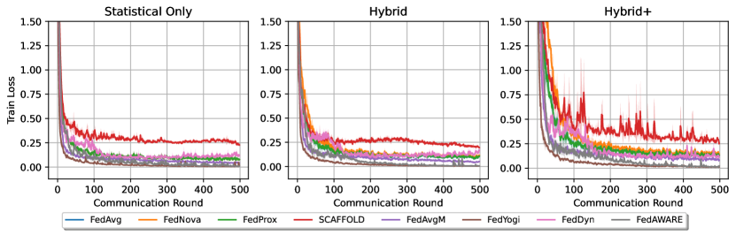
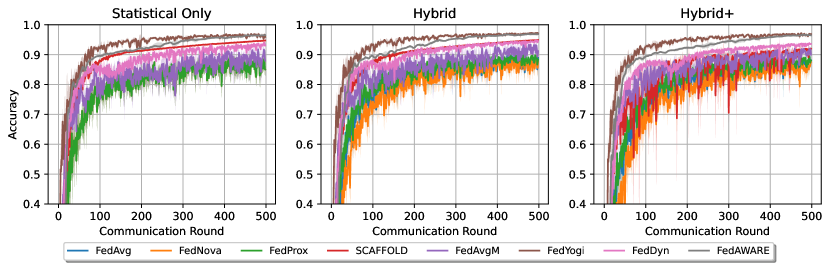
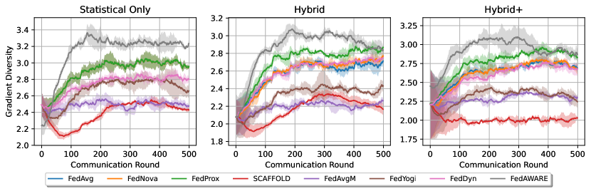
Figure 8: Train loss & test accuracy & gradient diversity of federated optimization algorithms on MNIST task.

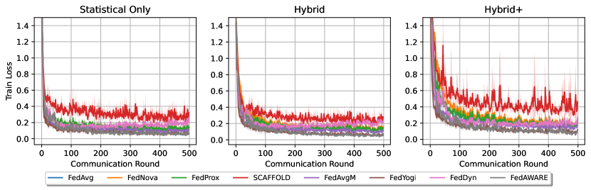
Figure 9: Train loss & test accuracy & gradient diversity of federated optimization algorithms on FashionMNIST task.

References

• Acar et al. (2020) Acar, D. A. E., Zhao, Y., Matas, R., Mattina, M., Whatmough, P., and Saligrama, V. Federated learning based on dynamic regularization. In International Conference on Learning Representations, 2020.
• Crawshaw et al. (2023) Crawshaw, M., Bao, Y., and Liu, M. Federated learning with client subsampling, data heterogeneity, and unbounded smoothness: A new algorithm and lower bounds. In Thirty-seventh Conference on Neural Information Processing Systems, 2023.
• Deng (2012) Deng, L. The mnist database of handwritten digit images for machine learning research. IEEE Signal Processing Magazine, 29(6):141–142, 2012.
• Haddadpour & Mahdavi (2019) Haddadpour, F. and Mahdavi, M. On the convergence of local descent methods in federated learning. arXiv preprint arXiv:1910.14425, 2019.
• Hsu et al. (2019) Hsu, T.-M. H., Qi, H., and Brown, M. Measuring the effects of non-identical data distribution for federated visual classification. arXiv preprint arXiv:1909.06335, 2019.
• Hu et al. (2022) Hu, Z., Shaloudegi, K., Zhang, G., and Yu, Y. Federated learning meets multi-objective optimization. IEEE Transactions on Network Science and Engineering, 9(4):2039–2051, 2022.
• Huang et al. (2023) Huang, M., Zhang, D., and Ji, K. Achieving linear speedup in non-iid federated bilevel learning. In ICML, volume 202 of Proceedings of Machine Learning Research, pp.  14039–14059. PMLR, 2023.
• Imteaj et al. (2021) Imteaj, A., Thakker, U., Wang, S., Li, J., and Amini, M. H. A survey on federated learning for resource-constrained iot devices. IEEE Internet of Things Journal, 9(1):1–24, 2021.
• Jaggi (2013) Jaggi, M. Revisiting frank-wolfe: Projection-free sparse convex optimization. In International conference on machine learning, pp.  427–435. PMLR, 2013.
• Kairouz et al. (2021) Kairouz, P., McMahan, H. B., Avent, B., Bellet, A., Bennis, M., Bhagoji, A. N., Bonawitz, K., Charles, Z., Cormode, G., Cummings, R., et al. Advances and open problems in federated learning. Foundations and Trends® in Machine Learning, 14(1–2):1–210, 2021.
• Karimireddy et al. (2020) Karimireddy, S. P., Kale, S., Mohri, M., Reddi, S., Stich, S., and Suresh, A. T. Scaffold: Stochastic controlled averaging for federated learning. In International Conference on Machine Learning, pp.  5132–5143. PMLR, 2020.
• Khaled et al. (2019) Khaled, A., Mishchenko, K., and Richtárik, P. First analysis of local gd on heterogeneous data. arXiv preprint arXiv:1909.04715, 2019.
• Krizhevsky et al. (2009) Krizhevsky, A., Hinton, G., et al. Learning multiple layers of features from tiny images. 2009.
• Li & Wang (2019) Li, D. and Wang, J. Fedmd: Heterogenous federated learning via model distillation. arXiv preprint arXiv:1910.03581, 2019.
• Li et al. (2023) Li, J., Li, A., Tian, C., Ho, Q., Xing, E. P., and Wang, H. Fednar: Federated optimization with normalized annealing regularization. arXiv preprint arXiv:2310.03163, 2023.
• Li et al. (2019) Li, T., Sanjabi, M., Beirami, A., and Smith, V. Fair resource allocation in federated learning. arXiv preprint arXiv:1905.10497, 2019.
• Li et al. (2020a) Li, T., Beirami, A., Sanjabi, M., and Smith, V. Tilted empirical risk minimization. In International Conference on Learning Representations, 2020a.
• Li et al. (2020b) Li, T., Sahu, A. K., Talwalkar, A., and Smith, V. Federated learning: Challenges, methods, and future directions. IEEE signal processing magazine, 37(3):50–60, 2020b.
• Li et al. (2020c) Li, T., Sahu, A. K., Zaheer, M., Sanjabi, M., Talwalkar, A., and Smith, V. Federated optimization in heterogeneous networks. Proceedings of Machine learning and systems, 2:429–450, 2020c.
• Liu et al. (2023) Liu, S., Lv, S., Zeng, D., Xu, Z., Wang, H., and Yu, Y. Personalized federated learning via amortized bayesian meta-learning. arXiv preprint arXiv:2307.02222, 2023.
• Ma et al. (2022) Ma, X., Zhu, J., Lin, Z., Chen, S., and Qin, Y. A state-of-the-art survey on solving non-iid data in federated learning. Future Generation Computer Systems, 135:244–258, 2022.
• Marfoq et al. (2021) Marfoq, O., Neglia, G., Bellet, A., Kameni, L., and Vidal, R. Federated multi-task learning under a mixture of distributions. Advances in Neural Information Processing Systems, 34:15434–15447, 2021.
• McMahan et al. (2017) McMahan, B., Moore, E., Ramage, D., Hampson, S., and y Arcas, B. A. Communication-efficient learning of deep networks from decentralized data. In Artificial intelligence and statistics, pp.  1273–1282. PMLR, 2017.
• Mohri et al. (2019) Mohri, M., Sivek, G., and Suresh, A. T. Agnostic federated learning. In International Conference on Machine Learning, pp.  4615–4625. PMLR, 2019.
• Reddi et al. (2020) Reddi, S., Charles, Z., Zaheer, M., Garrett, Z., Rush, K., Konečnỳ, J., Kumar, S., and McMahan, H. B. Adaptive federated optimization. arXiv preprint arXiv:2003.00295, 2020.
• Reddi et al. (2019) Reddi, S. J., Kale, S., and Kumar, S. On the convergence of adam and beyond. arXiv preprint arXiv:1904.09237, 2019.
• Sattler et al. (2020) Sattler, F., Müller, K.-R., and Samek, W. Clustered federated learning: Model-agnostic distributed multitask optimization under privacy constraints. IEEE transactions on neural networks and learning systems, 32(8):3710–3722, 2020.
• Sener & Koltun (2018) Sener, O. and Koltun, V. Multi-task learning as multi-objective optimization. Advances in neural information processing systems, 31, 2018.
• Smith et al. (2017) Smith, V., Chiang, C.-K., Sanjabi, M., and Talwalkar, A. S. Federated multi-task learning. Advances in neural information processing systems, 30, 2017.
• Tan et al. (2022) Tan, A. Z., Yu, H., Cui, L., and Yang, Q. Towards personalized federated learning. IEEE Transactions on Neural Networks and Learning Systems, 2022.
• Voigt & Von dem Bussche (2017) Voigt, P. and Von dem Bussche, A. The eu general data protection regulation (gdpr). A Practical Guide, 1st Ed., Cham: Springer International Publishing, 10(3152676):10–5555, 2017.
• Wang et al. (2020) Wang, J., Liu, Q., Liang, H., Joshi, G., and Poor, H. V. Tackling the objective inconsistency problem in heterogeneous federated optimization. Advances in neural information processing systems, 33:7611–7623, 2020.
• Wang et al. (2023) Wang, L., Guo, Y., Lin, T., and Tang, X. Delta: Diverse client sampling for fasting federated learning. In Thirty-seventh Conference on Neural Information Processing Systems, 2023.
• Wang et al. (2019) Wang, S., Tuor, T., Salonidis, T., Leung, K. K., Makaya, C., He, T., and Chan, K. Adaptive federated learning in resource constrained edge computing systems. IEEE journal on selected areas in communications, 37(6):1205–1221, 2019.
• Wu et al. (2023) Wu, X., Sun, J., Hu, Z., Zhang, A., and Huang, H. Solving a class of non-convex minimax optimization in federated learning. arXiv preprint arXiv:2310.03613, 2023.
• Xiao et al. (2017) Xiao, H., Rasul, K., and Vollgraf, R. Fashion-mnist: a novel image dataset for benchmarking machine learning algorithms. arXiv preprint arXiv:1708.07747, 2017.
• Xie et al. (2019) Xie, C., Koyejo, O., Gupta, I., and Lin, H. Local adaalter: Communication-efficient stochastic gradient descent with adaptive learning rates. arXiv preprint arXiv:1911.09030, 2019.
• Ye et al. (2023) Ye, R., Xu, M., Wang, J., Xu, C., Chen, S., and Wang, Y. Feddisco: Federated learning with discrepancy-aware collaboration. In ICML, volume 202 of Proceedings of Machine Learning Research, pp.  39879–39902. PMLR, 2023.
• Yin et al. (2018) Yin, D., Pananjady, A., Lam, M., Papailiopoulos, D., Ramchandran, K., and Bartlett, P. Gradient diversity: a key ingredient for scalable distributed learning. In International Conference on Artificial Intelligence and Statistics, pp.  1998–2007. PMLR, 2018.
• Zaheer et al. (2018) Zaheer, M., Reddi, S., Sachan, D., Kale, S., and Kumar, S. Adaptive methods for nonconvex optimization. Advances in neural information processing systems, 31, 2018.
• Zeng et al. (2023a) Zeng, D., Hu, X., Liu, S., Yu, Y., Wang, Q., and Xu, Z. Stochastic clustered federated learning. arXiv preprint arXiv:2303.00897, 2023a.
• Zeng et al. (2023b) Zeng, D., Liang, S., Hu, X., Wang, H., and Xu, Z. Fedlab: A flexible federated learning framework. Journal of Machine Learning Research, 24(100):1–7, 2023b. URL http://jmlr.org/papers/v24/22-0440.html.
• Zeng et al. (2022) Zeng, S., Li, Z., Yu, H., He, Y., Xu, Z., Niyato, D., and Yu, H. Heterogeneous federated learning via grouped sequential-to-parallel training. In International Conference on Database Systems for Advanced Applications, pp.  455–471. Springer, 2022.
• Zhang et al. (2023) Zhang, Y., Zeng, D., Luo, J., Xu, Z., and King, I. A survey of trustworthy federated learning with perspectives on security, robustness, and privacy. arXiv preprint arXiv:2302.10637, 2023.
• Zhao et al. (2018) Zhao, Y., Li, M., Lai, L., Suda, N., Civin, D., and Chandra, V. Federated learning with non-iid data. arXiv preprint arXiv:1806.00582, 2018.
• Zhou et al. (2022a) Zhou, S., Zhang, W., Jiang, J., Zhong, W., Gu, J., and Zhu, W. On the convergence of stochastic multi-objective gradient manipulation and beyond. In NeurIPS, 2022a.
• Zhou et al. (2022b) Zhou, S., Zhang, W., Jiang, J., Zhong, W., Gu, J., and Zhu, W. On the convergence of stochastic multi-objective gradient manipulation and beyond. Advances in Neural Information Processing Systems, 35:38103–38115, 2022b.
• Zhu et al. (2021) Zhu, Z., Hong, J., and Zhou, J. Data-free knowledge distillation for heterogeneous federated learning. In International conference on machine learning, pp.  12878–12889. PMLR, 2021.