Continual Contrastive Spoken Language Understanding

Abstract

Recently, neural networks have shown impressive progress across diverse fields, with speech processing being no exception. However, recent breakthroughs in this area require extensive offline training using large datasets and tremendous computing resources. Unfortunately, these models struggle to retain their previously acquired knowledge when learning new tasks continually, and retraining from scratch is almost always impractical. In this paper, we investigate the problem of learning sequence-to-sequence models for spoken language understanding in a class-incremental learning (CIL) setting and we propose COCONUT, a CIL method that relies on the combination of experience replay and contrastive learning. Through a modified version of the standard supervised contrastive loss applied only to the rehearsal samples, COCONUT preserves the learned representations by pulling closer samples from the same class and pushing away the others. Moreover, we leverage a multimodal contrastive loss that helps the model learn more discriminative representations of the new data by aligning audio and text features. We also investigate different contrastive designs to combine the strengths of the contrastive loss with teacher-student architectures used for distillation. Experiments on two established SLU datasets reveal the effectiveness of our proposed approach and significant improvements over the baselines. We also show that COCONUT can be combined with methods that operate on the decoder side of the model, resulting in further metrics improvements.

1 Introduction

With the rapid progress of intelligent voice-enabled personal assistants, the significance of Spoken Language Understanding (SLU) has gained substantial recognition in recent years (Arora et al., 2022; Qin et al., 2021). Conventional SLU models deploy a cascaded pipeline of an automatic speech recognition (ASR) system followed by a natural language understanding (NLU) module (Mesnil et al., 2014; Horlock & King, 2003). ASR maps the input speech into text representations, and NLU extracts the target intent labels from the intermediate text. Even though these approaches can leverage a vast abundance of ASR and NLU data, they suffer from ASR error propagation. Conversely, end-to-end (E2E) SLU (Agrawal et al., 2022; Lugosch et al., 2019; Saxon et al., 2021) has received more attention in recent research because it uses a single trainable model to map the speech audio directly to the intent labels, bypassing the need to explicitly generate a text transcript. This approach leads to reduced latency and error propagation.

The assumption that the data distribution the model will face after deployment aligns with what it encountered during the training phase is brittle and unrealistic. In fact, real-world scenarios entail evolving streams of data where novel categories (e.g., new vocabulary or intents) emerge sequentially, known as continual learning (CL). Unfortunately, while neural networks thrive in a stationary environment, the situation is reversed in CL, resulting in the “catastrophic forgetting” (CF) of the existing knowledge in favor of the fresh new information (McCloskey & Cohen, 1989). Although the majority of CL works have focused on computer vision tasks like image classification (Buzzega et al., 2020; Wang et al., 2022c) and semantic segmentation (Maracani et al., 2021; Yang et al., 2022a), a few works have recently turned their attention towards text (Wang et al., 2023a; Ke et al., 2023) and speech-related (Cappellazzo et al., 2023a; Diwan et al., 2023) problems, as well as vision-language (Ni et al., 2023; Zhu et al., 2023) and vision-audio (Mo et al., 2023; Pian et al., 2023).

While most SLU works have considered an offline setting, a thorough study of SLU under a class-incremental learning (CIL) setup still lacks. In CIL, one single model is adapted on a sequence of different tasks as incremental intent labels emerge sequentially. Recently, Cappellazzo et al. (2023b) studied the problem of CIL in ASR-SLU, where SLU is carried out in a sequence-to-sequence (seq2seq) fashion, thus computing the intent labels in an auto-regressive way together with the ASR transcriptions. By doing this, the model comprises three blocks: a text encoder, an audio encoder, and an ASR decoder. While Cappellazzo et al. (2023b) proposed to overcome CF by using knowledge distillation techniques applied to the ASR decoder, in this paper, we exploit the multi-modal audio-text setting and propose COCONUT: COntinual Contrastive spOken laNguage UndersTanding. COCONUT combines experience replay (ER) and contrastive learning principles. Whereas ER is a well-established approach in CL (Rolnick et al., 2019), only recently has contrastive learning been harnessed to learn representations continually. Both supervised (Cha et al., 2021; Yang et al., 2022a) and self-supervised (Fini et al., 2022; Wang et al., 2022c) contrastive learning have proven useful to lessen the CF issue. Specifically, COCONUT relies on two contrastive learning-based losses that operate on a shared embedding space where the audio and text features are projected.

The first contrastive loss, coined Negative-Student Positive-Teacher (NSPT), is a modified version of the supervised contrastive learning loss that aims to consolidate what the model has learned in the previous tasks. It also exploits the knowledge distillation (KD) principle (Hinton et al., 2015; Li & Hoiem, 2017) to guide the current model (student) to produce representations that follow the ones obtained with the model from the previous task (teacher). For this reason, this loss is computed only for the rehearsal data (i.e., the anchors). A key difference between our loss and the standard contrastive one is that the positive samples are computed using the teacher model (the positives only come from the rehearsal data), whereas the negatives are computed with the student. In this way, we avoid stale and scattered representations for the new data.

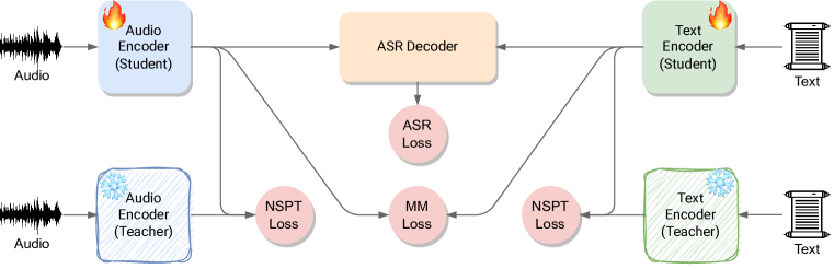
Figure 1: Overview of COCONUT: our proposed CL method. Aside from the standard ASR loss, COCONUT implements two contrastive learning-based losses. The NSPT (negative-student positive-teacher) loss is a supervised contrastive distillation loss that preserves the feature representations of the past classes for both audio and text samples. The positive and negative samples are computed with the teacher and student model, respectively. The MM (multi-modal) loss aims to align audio and text representations belonging to the same class. The combination of these two losses produces features that are more transferable and resilient to catastrophic forgetting.

The second loss is inspired by the recent progress in multi-modal representation learning. Considering that for audio-text paired data, audio and text represent the same information but in different ways, it has been shown that aligning their representations results in better performance for various speech-related problems (Zhu et al., 2022; Ye et al., 2022; Manco et al., 2022). Therefore, we propose a multi-modal (MM) supervised contrastive loss that, exclusively applied to the current task’s data, brings audio and text representations belonging to the same class into closer proximity in the shared feature space, resulting in features that are more transferable and resilient to CF. An overview of COCONUT is illustrated in Figure 1.

In summary, our contributions are the following:

• We introduce COCONUT, a CL method that makes use of two supervised contrastive learning objectives to mitigate catastrophic forgetting for seq2seq SLU models.

• We conduct extensive experiments on two popular SLU benchmarks and we show COCONUT achieves consistent improvements over the baselines. We also demonstrate that it can be combined with a KD technique applied to the ASR decoder, leading to further improvements.

• We finally ablate the contribution of each loss and its components, as well as the role of the temperature parameter in the contrastive continual learning process.

2 Related Work

A vast array of CL strategies exist in the literature (Wang et al., 2023b; Zhou et al., 2023), which can be categorized into some macro groups: regularization-based, experience replay, and architecture-based. Regularization methods contrast forgetting either by introducing some ad-hoc regularization terms that penalize changes to model weights (Ebrahimi et al., 2019; Kirkpatrick et al., 2017) or to model predictions (Hou et al., 2018; Li & Hoiem, 2017; Fini et al., 2020). Experience replay approaches interleave the new data with cherry-picked samples from the prior tasks (Chaudhry et al., 2018; Bang et al., 2021; Buzzega et al., 2020), or they incorporate regularization terms with this additional data to steer the optimization process and prevent catastrophic forgetting (Chaudhry et al., 2018; Wang et al., 2021; Yang et al., 2022b). Finally, architecture methods involve creating task-specific/adaptive parameters, such as dedicated parameters to each task (Xue et al., 2022; Wang et al., 2022a) or task-adaptive sub-modules or subnetworks (Aljundi et al., 2017; Ostapenko et al., 2021).

Contrastive learning (Oord et al., 2018; Chen et al., 2020) is a popular approach in self-supervised learning, but it can also be used in supervised learning (Gui et al., 2023) and multimodal learning (Radford et al., 2021). Its objective is to learn discriminative feature representations by pushing apart different samples (negatives) and bringing closer similar ones (positives). In the case of supervised CIL, it has been shown that endowing the model with contrastive learning objectives results in more robust representations against CF. For incremental semantic segmentation, Yang et al. (2022a) and Zhao et al. (2023) propose to exploit contrastive learning in conjunction with knowledge distillation. For image classification, Wang et al. (2022b) advance a contrastive learning strategy based on the vision transformer architecture for online CL.

3 Problem Formulation

3.1 ASR-SLU Multi-task Learning

SLU is considered a more difficult task than ASR and NLU since it involves concurrent acoustic and semantic interpretation (Tur & De Mori, 2011). For this reason, it is common practice in the literature to include an additional ASR objective such that the intent and the transcript are generated in an auto-regressive fashion, resulting in a multi-task learning setting (Arora et al., 2022; Peng et al., 2023). By doing this, the text transcript input to the model includes a class intent token that is specific to the actual task.

Let $\theta$ be the parameters of a seq2seq ASR model, constituted by an audio encoder, a text encoder (i.e., embedding layer), and an ASR decoder. Let $\textbf{x}=[x_{0},\dots,x_{U-1}]$ be an audio input sequence of length $U$, and $\textbf{y}=[y_{cls},y_{sep},y_{0},\dots,y_{J-3}]$ be the corresponding “extended” input transcript of length $J$, where with the term “extended” we refer to the original transcript $[y_{0},\dots,y_{J-3}]$ augmented with the intent class token $y_{cls}$ and a special separation token $y_{sep}$. The goal of the ASR model is to find the most likely extended transcript given the input sequence x:

$$\hat{\textbf{y}}=\operatorname*{arg\,max}_{\textbf{y}\in\mathcal{Y}^{*}}p(\textbf{y}|\textbf{x};\theta),$$ (1)

where $\mathcal{Y}^{*}$ is the set of all token sequences. The predicted intent is obtained extracting $y_{cls}$ from $\hat{\textbf{y}}$.

3.2 Class-Incremental Learning

For our experiments, we consider a CIL setting where we adapt a single model to learn sequentially $N$ tasks corresponding to non-overlapping subsets of classes (in our case intents). Put formally, the training dataset is divided into $N$ distinct tasks, $\mathcal{D}=\{\mathcal{D}_{0},\ldots,\mathcal{D}_{N-1}$}, based on the intent token $y_{cls}$, so that one intent is included in one and only one task. The dataset $\mathcal{D}_{n}$ of task $n$ comprises audio signals $\mathcal{X}_{n}$ with associated transcriptions $\mathcal{Y}_{n}$, i.e. $\mathcal{D}_{n}=(\mathcal{X}_{n},\mathcal{Y}_{n})$. The CIL setting is challenging in that the model must be able to distinguish all classes until task $n$, thus at inference time the task labels are not available (unlike in task-incremental learning) (Hsu et al., 2018).

4 Proposed Approach

4.1 Standard Rehearsal-based Approach

We assume the availability of a rehearsal buffer, $\mathcal{M}$, in which we can store a few samples for each class encountered in the previous tasks. During the training phase of task $n$, $\mathcal{D}_{n}$, we refer to $\mathcal{B}$ as a mini-batch of samples $(\textbf{x},\textbf{y})$, some of which come from the current task and some from the rehearsal memory. To increase the variance of the audio data, we apply SpecAug (Park et al., 2019) to the audio waveform x as a data augmentation transformation. Regarding the transcript y, we do not implement any augmentation technique. Then, we encode each modality separately through a dedicated feature encoder. An audio encoder maps each audio input into a feature vector $\textbf{h}_{\operatorname{A}}\in\mathbb{R}^{U\times d_{\operatorname{A}}}$, where $d_{\operatorname{A}}$ is the audio hidden size. Similarly, a text encoder converts each text input into a feature vector $\textbf{h}_{\operatorname{T}}\in\mathbb{R}^{J\times d_{\operatorname{T}}}$, where $d_{\operatorname{T}}$ is the text hidden size. At this point, if no specific CL losses are introduced, the ASR decoder generates the output sequence in an auto-regressive fashion, cross-attending on the audio encoder’s feature representations $\textbf{h}_{\operatorname{A}}$. Therefore, at task $n$, we minimize the conventional cross-entropy loss over the current mini-batch $\mathcal{B}$:

$$\mathcal{L}_{\text{ASR}}=-\frac{1}{|\mathcal{B}|}\sum_{(\textbf{x},\textbf{y})\in\mathcal{B}}\log(p(\textbf{y}|\textbf{x};\theta)).$$ (2)

4.2 COCONUT

Preliminaries. We introduce here some notations for our proposed approach COCONUT. Since we work with audio and text sequences, we need to aggregate the features we obtain with the encoders before computing the contrastive loss. For the audio component $\textbf{h}_{\operatorname{A}}$ we apply a mean operation over its sequence length, whereas for text we only select the feature related to the intent token. Then, as is common practice in contrastive learning (Radford et al., 2021; Chen et al., 2020), the resulting embeddings go through two separate linear projection layers that map them into a shared embedding space. At inference time, the projection layers are discarded. Therefore, we get the projected embeddings a and t in the following way:

$$\textbf{a}=g_{\operatorname{A}}(avg(\textbf{h}_{\operatorname{A}})),\quad\textbf{t}=g_{\operatorname{T}}(cls(\textbf{h}_{\operatorname{T}})),$$ (3)

where $cls(\cdot)$ is a function that extracts the feature associated with the class token, $g_{\operatorname{A}}(\cdot)$ and $g_{\operatorname{T}}(\cdot)$ are the projection layers, $\textbf{a}\in\mathbb{R}^{d_{\operatorname{S}}}$ and $\textbf{t}\in\mathbb{R}^{d_{\operatorname{S}}}$, where $d_{\operatorname{S}}$ is the dimension of the shared space.

Furthermore, we introduce some notations for the indices of samples coming from the current mini-batch $\mathcal{B}$. Let $\mathcal{I}_{c}$ and $\mathcal{I}_{r}$ represent the set of indices of the new task samples and the indices of the samples from the rehearsal memory (old task samples) in $\mathcal{B}$, respectively. Also, let $\mathcal{I}=\mathcal{I}_{c}\cup\mathcal{I}_{r}$, and we define $\mathcal{P}(k)$ as the set of indices of positive samples (i.e., samples with the same intent token).

Figure 2: Illustration of the NTPT loss and our proposed NSPT loss. Given an anchor sample from the current mini-batch, the NTPT loss computes the negatives and positives using the teacher model (dashed circles). Instead, the NSPT loss, since the negative samples mainly come from the new classes and the teacher model has not been trained using those classes, computes the positives with the teacher while the negatives are computed with the student model (solid circles). If the features obtained with the teacher are scattered and static (the teacher is frozen), those obtained with the student are more clustered and can be learned during the current task. Best viewed in color.

The objective of a standard supervised contrastive loss (SCL) (Khosla et al., 2020) is to push the representations of samples with different classes (negative pairs) farther apart while clustering representation of samples with the same class (positive pairs) closely together. Suppose that we get from the projection layers a generic representation $\textbf{z}_{i}^{D}$ for the $i$-th element in the batch, where $\textbf{z}=\{\textbf{a},\textbf{t}\}$ and the superscript $D$ denotes whether the representation is computed with the teacher or student model. A generic formulation of the SCL loss takes the following form:

$$\mathcal{L}_{\text{SCL}}=\sum_{k\in\mathcal{I}}\frac{-1}{|\mathcal{P}(k)|}\sum_{p\in\mathcal{P}(k)}\log\frac{\exp(\textbf{z}^{D}_{k}\cdot\textbf{z}^{D}_{p}/\tau)}{\sum_{i\in\mathcal{I}}\exp(\textbf{z}^{D}_{k}\cdot\textbf{z}^{D}_{i}/\tau)},$$ (4)

where $\tau\in\mathbb{R}^{+}$ is a fixed temperature scaling parameter.

Supervised Contrastive Distillation Loss (NSPT). This loss combines the benefits of knowledge distillation with those of contrastive learning (Tian et al., 2019; Sun et al., 2020). First of all, since the teacher model conveys information about the previous classes, we would like to use it as a guide for the student through a knowledge distillation objective. In this way, the loss encourages the student model to produce audio and text embeddings consistent with those obtained by the teacher. Therefore, only the rehearsal samples are involved in this process as the teacher had no chance to see the current data. Additionally, we want to pull closer embeddings sharing the same intent class (i.e. the positives), while we push away the others (i.e. the negatives, whose class is different). This is obtained via a modified version of the standard supervised contrastive loss tailored for our setting. In fact, a standard one would use the teacher model to compute both the positives and the negatives (Khosla et al., 2020). However, since the teacher model is frozen and it is pointless to compute the representations of the samples from the current task using the teacher, we propose to use the student model for computing the representations of the negatives. Therefore, our contrastive distillation loss computes the embeddings of the anchor and its corresponding negatives using the student model, while the positives come from the teacher (we call this loss Negative-Student Positive-Teacher, NSPT). On the contrary, for the standard contrastive loss both the positives and negatives are computed with the teacher (we call it Negative-Teacher Positive-Teacher, NTPT). Figure 2 illustrates visually how the NTPT and NSPT work in the shared embedding space. The NSPT loss is computed for both audio and text embeddings, leading to two components, one for each modality, as follows:

$$\mathcal{L}_{\text{NSPT}}=\sum_{k\in\mathcal{I}_{r}}\frac{-1}{|\mathcal{P}(k)|}\sum_{p\in\mathcal{P}(k)}\Biggl{[}\;\underbrace{\log\frac{\exp(\textbf{a}^{n}_{k}\cdot\textbf{a}^{n-1}_{p}/\tau)}{\sum_{i\in\mathcal{I}}\exp(\textbf{a}^{n}_{k}\cdot\textbf{a}^{n}_{i}/\tau)}}_{\mathcal{L}_{\text{A}}}+\underbrace{\log\frac{\exp(\textbf{t}^{n}_{k}\cdot\textbf{t}^{n-1}_{p}/\tau)}{\sum_{i\in\mathcal{I}}\exp(\textbf{t}^{n}_{k}\cdot\textbf{t}^{n}_{i}/\tau)}}_{\mathcal{L}_{\text{T}}}\;\Biggl{]},$$ (5)

where $n$ and $n-1$ denote whether the representation is obtained with the student or teacher, and $\mathcal{L}_{\text{A}}$ and $\mathcal{L}_{\text{T}}$ represent the audio and text contributions, respectively. We empirically validate that the intuition of using negative samples from the student is beneficial in practice in section 5.3.

Supervised Multi-Modal Contrastive Loss. This loss is introduced for two reasons. First of all, since during the first task (no CL) the NSPT loss is not computed, this means that the projector layers of the model are not trained. This is a problem during the second task when the student distills the knowledge from the teacher with randomly initialized projectors. Second, we want to exploit the multi-modal nature of our SLU CIL setting. Consequently, we introduce a multi-modal (MM) loss that aims to align audio and text representations belonging to the same class, and thus training the projectors of the model. This alignment is achieved via a supervised multi-modal (i.e., audio-text) contrastive learning objective where feature representations of samples sharing the same intent token are attracted while the others are pushed away. Similar to (Kwon et al., 2022), we use the [CLS] text token ($y_{cls}$) for performing the multi-modal alignment. Furthermore, following (Cha et al., 2021), we always treat the rehearsal samples as negatives, preventing them from being anchors during the learning process. This design choice is buttressed by two motivations: 1) rehearsal data have been learned by the previous model already and are preserved via the NSPT loss, and 2) we encourage the model to produce clusters for the new data that are separated from those of the rehearsal data. Formally, the MM loss takes the following form:

$$\mathcal{L}_{\text{MM}}=\sum_{k\in\mathcal{I}_{c}}\frac{-1}{|\mathcal{P}(k)|}\sum_{p\in\mathcal{P}(k)}\Biggl{[}\log\frac{\exp(\textbf{a}_{k}\cdot\textbf{t}_{p}/\tau)}{\sum_{i\in\mathcal{I}}\exp(\textbf{a}_{k}\cdot\textbf{t}_{i}/\tau)}+\log\frac{\exp(\textbf{t}_{k}\cdot\textbf{a}_{p}/\tau)}{\sum_{i\in\mathcal{I}}\exp(\textbf{t}_{k}\cdot\textbf{a}_{i}/\tau)}\Biggr{]}.$$ (6)

The first term of the internal loss is the audio-to-text component, whereas the second is the text-to-audio component (Zhang et al., 2022). The presence of both directions ($A\rightarrow T$ and $T\rightarrow A$) makes the MM loss symmetric. All in all, COCONUT minimizes the following loss:

$$\mathcal{L}=\mathcal{L}_{\text{ASR}}+\lambda_{\text{MM}}\mathcal{L}_{\text{MM}}+\lambda_{\text{NSPT}}\mathcal{L}_{\text{NSPT}},$$ (7)

where lambdas are loss-specific weights. An overview of COCONUT is illustrated in Figure 1.

5 Experiments

5.1 Experimental Setup and Implementation Details

Datasets and CIL setting. We evaluate COCONUT on two SLU datasets: the Fluent Speech Commands (FSC) (Lugosch et al., 2019) and the Spoken Language Understanding Resource Package (SLURP) (Bastianelli et al., 2020). FSC includes 30,043 English utterances, recorded at 16 kHz. It includes 31 intent classes in total. The SLURP dataset comprises around 56 hours of audio of people interacting with a home assistant (slurp_real), with the addition of 43.5 hours of synthetic data (slurp_synth). It is considered the most challenging SLU dataset due to its lexical complexity. Each utterance is annotated with 3 semantics: scenario, action, and entity. The pair (scenario, action) defines an intent. Overall, there are 18 scenarios and 69 intents. For our experiments, we only perform intent classification. Following (Cappellazzo et al., 2023b), we use the scenario labels as splitting criterion to define the CIL setting. We experiment on two configurations: 1) the datasets are partitioned into 3 tasks, each task comprising 6 scenarios for SLURP (denoted as SLURP-3), and 10 intents for FSC (FSC-3); 2) a more challenging configuration with 6 tasks, each task including 3 scenarios for SLURP (SLURP-6), and 5 intents for FSC (FSC-6).

Implementation Details. For both datasets, the text encoder is a standard text embedding layer with size $768$. For the audio encoder, we use a Wav2vec 2.0 base model (Baevski et al., 2020) pre-trained and fine-tuned on 960 hours of Librispeech for SLURP ($\sim 94.3$M parameters), while we use DistilHuBERT base (Chang et al., 2022) for FSC ($\sim 23.5$M parameters). Since FSC is a less challenging dataset than SLURP, we found that a smaller pre-trained encoder is sufficient to achieve state-of-the-art results. Both encoders have hidden sizes of $768$ and their feature extractor is kept frozen during training. As in (Radford et al., 2021), we employ linear projection layers to map from each encoder’s representation to the audio-text embedding space, whose dimension is $512$. The ASR decoder is transformer-based with $6$ layers, hidden size equal to $768$, $8$ attention heads, and the dimension of the feedforward layers is $2048$.

For the tokenization we apply Byte-Pair Encoding (BPE) (Sennrich et al., 2016) for SLURP, with a vocabulary size of $1000$ and BPE dropout equal to $0.1$, whereas for FSC, given the limited number of unique words, we use word tokenization, resulting in 139 tokens. BPE automatically assigns to each intent a dedicated token, whereas for FSC we manually add the intent tokens. We refer the reader to the appendix for an exhaustive description of the hyperparameters. Regarding the weight coefficients, we set $\lambda_{\text{MM}}$ to $0.1$, and similar to (Douillard et al., 2022; Wu et al., 2019) we set $\lambda_{\text{NSPT}}$ to $\frac{L_{p}}{L_{p}+L_{n}}$, where $L_{p}$ and $L_{n}$ count the number of past and new classes.

Baselines. Apart from the standard offline (1 task, no continual) and fine-tuning (no CL strategies) baselines, we compare COCONUT against standard experience replay (ER) methods with random and iCaRL (Rebuffi et al., 2017) sampling strategies. We note that ER is already a strong baseline for FSC and SLURP. Additionally, we report two methods proposed in (Cappellazzo et al., 2023b): audio-KD (A-KD) that applies the KD on the audio features of the rehearsal samples, and seq-KD (S-KD) that at the end of the current task stores the text transcriptions computed with beam search for the rehearsal samples and use them as pseudo-transcriptions for the next task. This method operates on the ASR decoder. We also report text-KD (T-KD), the text counterpart of the A-KD.

Metrics. Following (Douillard et al., 2022), we report the results in terms of the Avg Acc, which is the average of the intent accuracies after each training task, and the Last Acc, which is the intent accuracy after the last task. We also report the Avg WER, defined as the average of the Word Error Rate (WER) of the extended transcription after each task.

5.2 Main Results

Table 1: Results in terms of Average Accuracy ($\uparrow$), Last Accuracy ($\uparrow$), and Average WER ($\downarrow$) for different strategies on FSC and SLURP datasets. The second column represents the experience replay (ER) buffer size and the selection strategy (Selec.) used to populate the buffer. Bold and underscore numbers denote the best and second best method for a specific setting and metric, respectively. We show in the last row that COCONUT and S-KD can be used together, leading to the best results. For simplicity, the values of the last row are not in bold even though attain the best results.

Setting $\rightarrow$ FSC-3 FSC-6 SLURP-3 SLURP-6 ————————— ————————— ————————— ————————— Metric $\rightarrow$ ER size/ Avg Last Avg Avg Last Avg Avg Last Avg Avg Last Avg Method $\downarrow$ Selec. Acc Acc WER Acc Acc WER Acc Acc WER Acc Acc WER Offline - 99.28 - 0.48 99.28 - 0.48 84.41 - 17.65 84.41 - 17.65 Fine-tuning - 49.13 17.61 36.37 29.92 7.59 54.66 46.65 18.42 28.32 31.90 10.57 34.79 ER 2% / rand 88.02 84.20 9.19 81.19 79.71 13.75 75.62 68.68 19.55 72.75 68.49 22.98 ER 1% / rand 79.17 69.81 15.87 68.61 63.71 24.04 71.44 61.88 21.25 66.57 58.22 24.50 ER 1% / iCaRL 82.04 74.00 13.45 69.76 64.12 23.22 71.94 63.22 21.06 68.08 62.29 26.05 T-KD 1% / iCaRL 82.11 75.43 12.95 69.08 64.73 23.82 72.44 62.43 21.19 66.95 60.47 24.26 A-KD 1% / iCaRL 84.79 78.12 11.54 73.54 67.05 20.36 72.10 63.84 20.67 68.52 62.51 24.29 S-KD 1% / iCaRL 84.29 75.31 12.39 73.65 67.71 21.27 74.28 65.95 21.26 69.91 63.22 24.26 COCONUT 1% / iCaRL 86.39 80.21 11.08 77.09 73.80 19.05 72.75 64.62 21.25 70.17 63.66 24.29 COCONUT +S-KD 1% / iCaRL 87.64 80.45 10.49 77.57 74.01 18.47 75.58 67.39 20.61 71.91 65.41 24.16

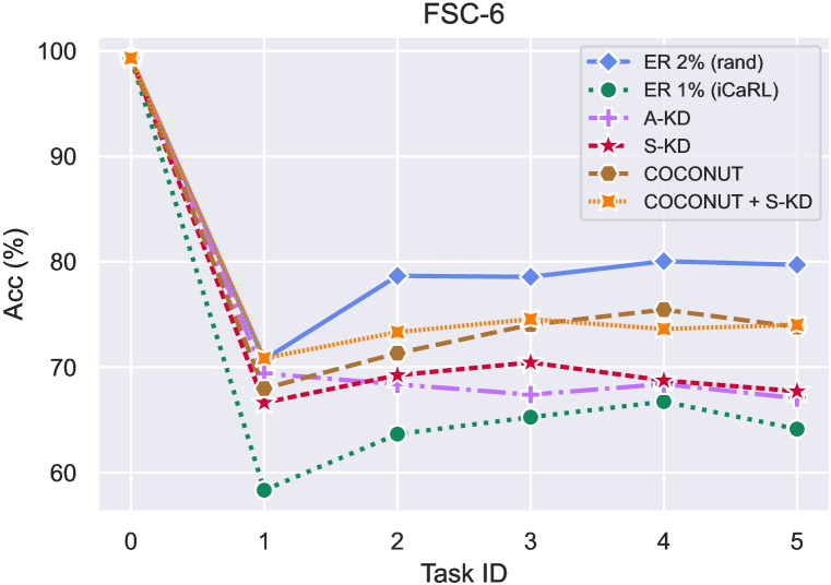
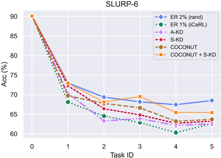
Figure 3: Left: the trend of the intent accuracy on the observed tasks for the FSC-6 setting. Right: the trend of the intent accuracy on the observed tasks for SLURP-6.

In the first two rows of Table 1, we include the upper and lower bounds represented by the offline learning (which is in line with the state-of-the-art) and fine-tuning approaches. For the fine-tuning approach, we can notice how CF deteriorates the knowledge of the prior classes. We then include ER baselines with buffer capacity equal to 1 or 2% of the dataset size. While all methods use 1%, we also include one with 2% to show how COCONUT and the other methods perform with respect to this one, but using half memory. From these results we can see that ER-based methods achieve good results for all metrics and configurations, confirming themselves as solid baselines. For FSC, COCONUT outperforms the other baselines by a significant margin, in terms of both accuracy and WER. Its combination with the S-KD leads to additional improvements (last row).

If we turn our focus to SLURP we see that, for the setting with 3 tasks, S-KD turns out to be the best approach in terms of intent accuracy, followed by COCONUT. For the WER, all the methods achieve similar performance and do not provide significant enhancements. We speculate that, as only some words are task-specific while the others are spread across multiple tasks, the text modality is less affected by CF. It is also compelling to note that the A-KD always achieves better performance than T-KD, a trend that will also be observed for the NSPT loss in the ablation study. For SLURP-6, COCONUT slightly surpasses S-KD in terms of accuracy, and performs on par with the others for the WER metric. This indicates that COCONUT scales properly with the number of tasks, and thus the setting becomes more challenging. Additionally, we point out that for SLURP COCONUT provides less noticeable improvements than FSC. This can be attributable to the higher complexity of the dataset due to its larger dictionary and to the larger number of intents with respect to FSC (69 vs. 31). Finally, similar to FSC, the combination of COCONUT with S-KD attains the best results, confirming that fighting CF both at the encoders and ASR decoder is an effective solution.

In Fig. 3 we illustrate the trend of the intent accuracy after each task for FSC-6 and SLURP-6, respectively. For FSC-6, COCONUT outperforms the other baselines by a large margin after each task. For SLURP-6, COCONUT has a similar trend as S-KD, and their combination leads to a noteworthy boost to such an extent that after task 3 it even beats the baseline that uses twice as much memory. On the left part of Fig. 4 we show the trend of the WER task by task. If it is evident that COCONUT and its combination with S-KD outstrip the other baselines, we can also observe that the gap between COCONUT and the baseline with 2% of rehearsal samples is more prominent for the WER than it was for the accuracy. On the right of Fig. 4, we study the trend of COCONUT for different values of rehearsal samples per class. Note that 8 samples per class is tantamount to a buffer of capacity 1% with respect to the entire training dataset. The maximum gain provided by COCNUT with respect to the ER baseline is reached for 4 and 8 samples per class ($9.27$ and $6.69$, respectively), while for the extreme cases of 2 and 16 samples, the gap is reduced. This is explained by the fact that when few samples are stored for each class, the effect of the NSPT loss is highly reduced given its reliance on the rehearsal data, whilst in the opposite case the abundance of rehearsal data makes the ER baseline already strong, thereby improving it becomes more challenging.

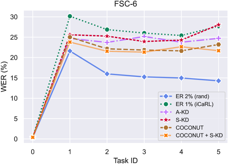
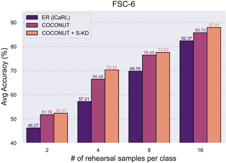
Figure 4: Left: the trend of the WER on the observed tasks for the FSC-6 setting. Right: the accuracy of COCONUT and other methods as a function of the memory size.

Table 2: Ablation on the use of NSPT and NTPT losses.

Dataset $\rightarrow$	FSC-6			SLURP-6
Metric $\rightarrow$	Avg	Last	Avg	Avg	Last	Avg
Method $\downarrow$	Acc	Acc	WER	Acc	Acc	WER
ER 1%/iCaRL	69.76	64.12	23.22	68.08	62.29	26.05
MM	71.12	67.76	22.88	68.78	62.94	24.81
MM + NTPT	74.05	67.61	21.22	68.91	62.57	24.69
MM + NSPT	77.09	73.80	19.05	70.17	63.66	24.29

5.3 Ablation Study

In this section, we ablate some design properties of COCONUT. In Tab. 2 we evaluate the difference in performance between the standard NTPT loss and our proposed NSPT. For FSC-6, the use of our proposed NSPT loss gives a considerable improvement over the NTPT loss in terms of all three considered metrics. For SLURP-6, the trend is maintained, and now the NTPT even brings a small deterioration over the MM baseline in terms of Last Acc. Also, the MM loss alone contributes positively over the ER baseline for both settings. We recall that we do not study the individual contribution of the NSPT loss due to the issue of the randomly-initialized projectors of the teacher during the second task (see section 4.2). In Table 5.3 we study the design properties of the MM loss on FSC-6, and with its best configuration, we determine the individual contribution of the audio and text components to the NSPT loss. As was evident for the A-KD and T-KD, with the former giving more valuable results, here we also discover that the audio component is predominant. Plus, the concurrent use of both components brings a moderate increase in accuracy, and this is due to the alignment between audio and text obtained via the MM loss.

Table 3: Ablation study of the MM (upper part) and NSPT (bottom part) components. CLS: whether only the intent class token is used; Anchor: whether ER data are excluded from the anchors. $\mathcal{L}_{\text{A}}/\mathcal{L}_{\text{T}}$: whether the audio/text component of NSPT loss is used.

CLS	Anchor	$\mathcal{L}_{\text{A}}$	$\mathcal{L}_{\text{T}}$	Acc
				70.10
✓				70.49
	✓			71.09
✓	✓			71.12
✓	✓	✓		76.84
✓	✓		✓	73.11
✓	✓	✓	✓	77.09

Table 4: Ablation study of the temperature $\tau$ for the MM loss. We experiment on FSC-6 by setting $\tau$ beforehand and making it a learnable hyperparameter as is common practice in offline settings (Radford et al., 2021). The light-blue row corresponds to the value we used for our experiments.

Metric $\rightarrow$	Avg	Last	Avg
Temp. ($\tau$) $\downarrow$	Acc	Acc	WER
0.07	71.06	64.75	22.07
0.1	71.12	67.76	22.88
0.2	71.01	62.35	22.78
Learnable	69.05	66.33	24.57

On the impact of the temperature parameter. Finally, in this section we analyze the role of the temperature parameter in the CIL process for the MM loss (see Eq. 6) on the FSC-6 setting. We first try to set the value beforehand ($0.07$, $0.1$, $0.2$), and then we make the temperature a learnable hyperparameter (initial value is $0.07$). Results are reported in Table 5.3. We can observe that $\tau=0.1$ is the best configuration for the accuracy metric. Note that, however, the model does not seem very sensible to the temperature for the Avg Acc, whereas the Last Acc is more influenced. Since the Avg Acc does not change much across the three configurations, yet the Last Acc sways much more, this means that for $\tau=0.1$ the model struggles more during the initial tasks, but it performs better towards the end of the learning process. On the other hand, learning $\tau$ task by task does not seem to be the right choice as the Avg Acc and WER metrics deteriorate with respect to the other three configurations where it is fixed. In fact, we observed that during the first tasks, the model is learning the optimal value for $\tau$ until it finds it (this value approximately lies in the range $0.134-0.142$). This initial transitional phase penalizes the accuracy of the first tasks, which in turn leads to a deterioration in the Avg Acc metric.

6 Conclusion

In this work, we study the problem of E2E SLU using a seq-2-seq model for class-incremental learning. In order to mitigate catastrophic forgetting we propose COCONUT, a CL approach that exploits experience replay and contrastive learning. On the one hand, it preserves the previously learned feature representations via an ad-hoc supervised contrastive distillation loss, on the other it contributes to aligning audio and text representations, thus resulting in more transferable and robust to catastrophic forgetting representations. We also show that COCONUT outperforms the other baselines and that synergizes with other knowledge distillation techniques operating on the decoder side. We finally dissect the design choices of COCONUT through specific ablation studies, as well as the influence of the temperature parameter throughout the continual learning process.

Appendix A Supplementary Material

A.1 Hyperparameters

We list the main hyperparameters used for our experiments in table 5. We also mention the number of epochs for each setting. For FSC-3, the number of epochs for each task is {40,30,30}, while for SLURP-3 we have {40,25,25}. For FSC-6 and SLURP-6 we use {40,30,30,30,30,30} and {40,25,20,20,20,20} epochs, respectively. We finally note that we set lr = $5\cdot 10^{-4}$ for the text encoder, the ASR decoder and the classifier, while for the audio encoder we set a smaller learning rate, lr = $5\cdot 10^{-5}$, because it is pre-trained.

Table 5: Training hyperparameters for FSC and SLURP.

Hyperparameter	FSC		SLURP
Batch Size		$32$
Optimizer		AdamW
$\beta_{1}$		$0.9$
$\beta_{2}$		$0.98$
$\epsilon$		$10^{-6}$
lr		$5\cdot 10^{-4}$
Weight Decay		$0.1$
Tokenizer	Word Tok.		BPE Tok.
Beam Search width	5		20
Temperature $\tau$		$0.1$

A.2 SpecAug details

In this section, we elaborate on the use of SpecAug for augmenting the audio input data. SpecAug (Park et al., 2019) is a popular augmentation technique that is applied directly on the log mel spectrogram of an audio signal, with the aim of making the model invariant to features deformation. In the original paper, they advance three different types of distortions: time warping, and time and frequency masking, where blocks of consecutive time steps and frequency channels are zero-masked, respectively. Since our audio encoders (i.e., DistilHuBERT and Wav2vec 2.0) work on the raw audio waveforms, SpecAug is not applicable by default. In order to circumvent this problem, we apply an approximated version of SpecAug directly to the raw waveform, as proposed in the SpeechBrain library (Ravanelli et al., 2021). We randomly drop chunks of the audio waveform (by zero-masking) and frequency bands (with band-drop filters). Unlike the SpeechBrain implementation, we do not apply speed perturbation. In more detail, with probability $0.5$ we randomly drop up to $2$ frequencies, while with probability $0.5$ we randomly drop up to $3$ chunks of audio whose length is sampled from a uniform distribution $\sim\mathcal{U}(0,0.05\cdot len(x))$, where $len(x)$ is the length of the considered audio waveform $x$.

A.3 Limitations

Our work comes with some limitations. First of all, the number of suitable SLU datasets for defining a CIL setting is limited since few datasets provide enough intent classes. Then, we could not use batches larger than $32$ owing to computational limitations, and it is known that contrastive learning benefits from larger batches.

A.4 Future Work

COCONUT relies on two contrastive learning-based losses applied to the projections of audio and text encoders outputs. In principle, COCONUT could be exploited in other multi-modal settings such as audio-vision or vision-language. Therefore, it would be interesting to study whether COCONUT can be exploited in other different multi-modal scenarios. Also, since these settings usually involve a larger number of classes than ours, we would be able to test how COCONUT scales to the number of tasks.

References

- Agrawal et al. (2022) Bhuvan Agrawal, Markus Müller, Samridhi Choudhary, Martin Radfar, Athanasios Mouchtaris, Ross McGowan, Nathan Susanj, and Siegfried Kunzmann. Tie your embeddings down: Cross-modal latent spaces for end-to-end spoken language understanding. In ICASSP 2022-2022 IEEE International Conference on Acoustics, Speech and Signal Processing (ICASSP), pp. 7157–7161. IEEE, 2022.
- Aljundi et al. (2017) Rahaf Aljundi, Punarjay Chakravarty, and Tinne Tuytelaars. Expert gate: Lifelong learning with a network of experts. In Proceedings of the IEEE Conference on Computer Vision and Pattern Recognition, pp. 3366–3375, 2017.
- Arora et al. (2022) Siddhant Arora, Siddharth Dalmia, Pavel Denisov, Xuankai Chang, Yushi Ueda, Yifan Peng, Yuekai Zhang, Sujay Kumar, Karthik Ganesan, Brian Yan, et al. Espnet-slu: Advancing spoken language understanding through espnet. In ICASSP 2022-2022 IEEE International Conference on Acoustics, Speech and Signal Processing (ICASSP), pp. 7167–7171. IEEE, 2022.
- Baevski et al. (2020) Alexei Baevski, Yuhao Zhou, Abdelrahman Mohamed, and Michael Auli. wav2vec 2.0: A framework for self-supervised learning of speech representations. Advances in neural information processing systems, 33:12449–12460, 2020.
- Bang et al. (2021) Jihwan Bang, Heesu Kim, YoungJoon Yoo, Jung-Woo Ha, and Jonghyun Choi. Rainbow memory: Continual learning with a memory of diverse samples. In Proceedings of the IEEE/CVF Conference on Computer Vision and Pattern Recognition, pp. 8218–8227, 2021.
- Bastianelli et al. (2020) Emanuele Bastianelli, Andrea Vanzo, Pawel Swietojanski, and Verena Rieser. Slurp: A spoken language understanding resource package. arXiv preprint arXiv:2011.13205, 2020.
- Buzzega et al. (2020) Pietro Buzzega, Matteo Boschini, Angelo Porrello, Davide Abati, and Simone Calderara. Dark experience for general continual learning: a strong, simple baseline. Advances in neural information processing systems, 33:15920–15930, 2020.
- Cappellazzo et al. (2023a) Umberto Cappellazzo, Daniele Falavigna, and Alessio Brutti. An investigation of the combination of rehearsal and knowledge distillation in continual learning for spoken language understanding. Interspeech, 2023a.
- Cappellazzo et al. (2023b) Umberto Cappellazzo, Muqiao Yang, Daniele Falavigna, and Alessio Brutti. Sequence-level knowledge distillation for class-incremental end-to-end spoken language understanding. Interspeech, 2023b.
- Cha et al. (2021) Hyuntak Cha, Jaeho Lee, and Jinwoo Shin. Co2l: Contrastive continual learning. In Proceedings of the IEEE/CVF International conference on computer vision, pp. 9516–9525, 2021.
- Chang et al. (2022) Heng-Jui Chang, Shu-wen Yang, and Hung-yi Lee. Distilhubert: Speech representation learning by layer-wise distillation of hidden-unit bert. In ICASSP 2022-2022 IEEE International Conference on Acoustics, Speech and Signal Processing (ICASSP), pp. 7087–7091. IEEE, 2022.
- Chaudhry et al. (2018) Arslan Chaudhry, Marc’Aurelio Ranzato, Marcus Rohrbach, and Mohamed Elhoseiny. Efficient lifelong learning with a-gem. arXiv preprint arXiv:1812.00420, 2018.
- Chen et al. (2020) Ting Chen, Simon Kornblith, Mohammad Norouzi, and Geoffrey Hinton. A simple framework for contrastive learning of visual representations. In International conference on machine learning, pp. 1597–1607. PMLR, 2020.
- Diwan et al. (2023) Anuj Diwan, Ching-Feng Yeh, Wei-Ning Hsu, Paden Tomasello, Eunsol Choi, David Harwath, and Abdelrahman Mohamed. Continual learning for on-device speech recognition using disentangled conformers. In ICASSP 2023-2023 IEEE International Conference on Acoustics, Speech and Signal Processing (ICASSP), pp. 1–5. IEEE, 2023.
- Douillard et al. (2022) Arthur Douillard, Alexandre Ramé, Guillaume Couairon, and Matthieu Cord. Dytox: Transformers for continual learning with dynamic token expansion. In Proceedings of the IEEE/CVF Conference on Computer Vision and Pattern Recognition, pp. 9285–9295, 2022.
- Ebrahimi et al. (2019) Sayna Ebrahimi, Mohamed Elhoseiny, Trevor Darrell, and Marcus Rohrbach. Uncertainty-guided continual learning with bayesian neural networks. arXiv preprint arXiv:1906.02425, 2019.
- Fini et al. (2020) Enrico Fini, Stéphane Lathuiliere, Enver Sangineto, Moin Nabi, and Elisa Ricci. Online continual learning under extreme memory constraints. In Computer Vision–ECCV 2020: 16th European Conference, Glasgow, UK, August 23–28, 2020, Proceedings, Part XXVIII 16, pp. 720–735. Springer, 2020.
- Fini et al. (2022) Enrico Fini, Victor G Turrisi Da Costa, Xavier Alameda-Pineda, Elisa Ricci, Karteek Alahari, and Julien Mairal. Self-supervised models are continual learners. In Proceedings of the IEEE/CVF Conference on Computer Vision and Pattern Recognition, pp. 9621–9630, 2022.
- Gui et al. (2023) Jie Gui, Tuo Chen, Qiong Cao, Zhenan Sun, Hao Luo, and Dacheng Tao. A survey of self-supervised learning from multiple perspectives: Algorithms, theory, applications and future trends. arXiv preprint arXiv:2301.05712, 2023.
- Hinton et al. (2015) Geoffrey Hinton, Oriol Vinyals, and Jeff Dean. Distilling the knowledge in a neural network. arXiv preprint arXiv:1503.02531, 2015.
- Horlock & King (2003) James Horlock and Simon King. Discriminative methods for improving named entity extraction on speech data. In Proc. 8th European Conference on Speech Communication and Technology (Eurospeech 2003), pp. 2765–2768, 2003. doi: 10.21437/Eurospeech.2003-737.
- Hou et al. (2018) Saihui Hou, Xinyu Pan, Chen Change Loy, Zilei Wang, and Dahua Lin. Lifelong learning via progressive distillation and retrospection. In Proceedings of the European Conference on Computer Vision (ECCV), pp. 437–452, 2018.
- Hsu et al. (2018) Yen-Chang Hsu, Yen-Cheng Liu, Anita Ramasamy, and Zsolt Kira. Re-evaluating continual learning scenarios: A categorization and case for strong baselines. arXiv preprint arXiv:1810.12488, 2018.
- Ke et al. (2023) Zixuan Ke, Yijia Shao, Haowei Lin, Tatsuya Konishi, Gyuhak Kim, and Bing Liu. Continual learning of language models. arXiv preprint arXiv:2302.03241, 2023.
- Khosla et al. (2020) Prannay Khosla, Piotr Teterwak, Chen Wang, Aaron Sarna, Yonglong Tian, Phillip Isola, Aaron Maschinot, Ce Liu, and Dilip Krishnan. Supervised contrastive learning. Advances in neural information processing systems, 33:18661–18673, 2020.
- Kirkpatrick et al. (2017) James Kirkpatrick, Razvan Pascanu, Neil Rabinowitz, Joel Veness, Guillaume Desjardins, Andrei A Rusu, Kieran Milan, John Quan, Tiago Ramalho, Agnieszka Grabska-Barwinska, et al. Overcoming catastrophic forgetting in neural networks. Proceedings of the national academy of sciences, 114(13):3521–3526, 2017.
- Kwon et al. (2022) Gukyeong Kwon, Zhaowei Cai, Avinash Ravichandran, Erhan Bas, Rahul Bhotika, and Stefano Soatto. Masked vision and language modeling for multi-modal representation learning. arXiv preprint arXiv:2208.02131, 2022.
- Li & Hoiem (2017) Zhizhong Li and Derek Hoiem. Learning without forgetting. IEEE transactions on pattern analysis and machine intelligence, 40(12):2935–2947, 2017.
- Lugosch et al. (2019) Loren Lugosch, Mirco Ravanelli, Patrick Ignoto, Vikrant Singh Tomar, and Yoshua Bengio. Speech model pre-training for end-to-end spoken language understanding. arXiv preprint arXiv:1904.03670, 2019.
- Manco et al. (2022) Ilaria Manco, Emmanouil Benetos, Elio Quinton, and György Fazekas. Contrastive audio-language learning for music. arXiv preprint arXiv:2208.12208, 2022.
- Maracani et al. (2021) Andrea Maracani, Umberto Michieli, Marco Toldo, and Pietro Zanuttigh. Recall: Replay-based continual learning in semantic segmentation. In Proceedings of the IEEE/CVF international conference on computer vision, pp. 7026–7035, 2021.
- McCloskey & Cohen (1989) Michael McCloskey and Neal J Cohen. Catastrophic interference in connectionist networks: The sequential learning problem. In Psychology of learning and motivation, volume 24, pp. 109–165. Elsevier, 1989.
- Mesnil et al. (2014) Grégoire Mesnil, Yann Dauphin, Kaisheng Yao, Yoshua Bengio, Li Deng, Dilek Hakkani-Tur, Xiaodong He, Larry Heck, Gokhan Tur, Dong Yu, et al. Using recurrent neural networks for slot filling in spoken language understanding. IEEE/ACM Transactions on Audio, Speech, and Language Processing, 23(3):530–539, 2014.
- Mo et al. (2023) Shentong Mo, Weiguo Pian, and Yapeng Tian. Class-incremental grouping network for continual audio-visual learning. arXiv preprint arXiv:2309.05281, 2023.
- Ni et al. (2023) Zixuan Ni, Longhui Wei, Siliang Tang, Yueting Zhuang, and Qi Tian. Continual vision-language representaion learning with off-diagonal information. arXiv preprint arXiv:2305.07437, 2023.
- Oord et al. (2018) Aaron van den Oord, Yazhe Li, and Oriol Vinyals. Representation learning with contrastive predictive coding. arXiv preprint arXiv:1807.03748, 2018.
- Ostapenko et al. (2021) Oleksiy Ostapenko, Pau Rodriguez, Massimo Caccia, and Laurent Charlin. Continual learning via local module composition. Advances in Neural Information Processing Systems, 34:30298–30312, 2021.
- Park et al. (2019) Daniel S Park, William Chan, Yu Zhang, Chung-Cheng Chiu, Barret Zoph, Ekin D Cubuk, and Quoc V Le. Specaugment: A simple data augmentation method for automatic speech recognition. arXiv preprint arXiv:1904.08779, 2019.
- Peng et al. (2023) Yifan Peng, Siddhant Arora, Yosuke Higuchi, Yushi Ueda, Sujay Kumar, Karthik Ganesan, Siddharth Dalmia, Xuankai Chang, and Shinji Watanabe. A study on the integration of pre-trained ssl, asr, lm and slu models for spoken language understanding. In 2022 IEEE Spoken Language Technology Workshop (SLT), pp. 406–413. IEEE, 2023.
- Pian et al. (2023) Weiguo Pian, Shentong Mo, Yunhui Guo, and Yapeng Tian. Audio-visual class-incremental learning. ICCV, 2023.
- Qin et al. (2021) Libo Qin, Tianbao Xie, Wanxiang Che, and Ting Liu. A survey on spoken language understanding: Recent advances and new frontiers. arXiv preprint arXiv:2103.03095, 2021.
- Radford et al. (2021) Alec Radford, Jong Wook Kim, Chris Hallacy, Aditya Ramesh, Gabriel Goh, Sandhini Agarwal, Girish Sastry, Amanda Askell, Pamela Mishkin, Jack Clark, et al. Learning transferable visual models from natural language supervision. In International conference on machine learning, pp. 8748–8763. PMLR, 2021.
- Ravanelli et al. (2021) Mirco Ravanelli, Titouan Parcollet, Peter Plantinga, Aku Rouhe, Samuele Cornell, Loren Lugosch, Cem Subakan, Nauman Dawalatabad, Abdelwahab Heba, Jianyuan Zhong, et al. Speechbrain: A general-purpose speech toolkit. arXiv preprint arXiv:2106.04624, 2021.
- Rebuffi et al. (2017) Sylvestre-Alvise Rebuffi, Alexander Kolesnikov, Georg Sperl, and Christoph H Lampert. iCaRL: Incremental classifier and representation learning. In Proceedings of the IEEE conference on Computer Vision and Pattern Recognition, pp. 2001–2010, 2017.
- Rolnick et al. (2019) David Rolnick, Arun Ahuja, Jonathan Schwarz, Timothy Lillicrap, and Gregory Wayne. Experience replay for continual learning. Advances in Neural Information Processing Systems, 32, 2019.
- Saxon et al. (2021) Michael Saxon, Samridhi Choudhary, Joseph P McKenna, and Athanasios Mouchtaris. End-to-end spoken language understanding for generalized voice assistants. arXiv preprint arXiv:2106.09009, 2021.
- Sennrich et al. (2016) Rico Sennrich, Barry Haddow, and Alexandra Birch. Neural machine translation of rare words with subword units. In Proceedings of the 54th Annual Meeting of the Association for Computational Linguistics (Volume 1: Long Papers), pp. 1715–1725, 2016.
- Sun et al. (2020) Siqi Sun, Zhe Gan, Yu Cheng, Yuwei Fang, Shuohang Wang, and Jingjing Liu. Contrastive distillation on intermediate representations for language model compression. arXiv preprint arXiv:2009.14167, 2020.
- Tian et al. (2019) Yonglong Tian, Dilip Krishnan, and Phillip Isola. Contrastive representation distillation. arXiv preprint arXiv:1910.10699, 2019.
- Tur & De Mori (2011) Gokhan Tur and Renato De Mori. Spoken language understanding: Systems for extracting semantic information from speech. John Wiley & Sons, 2011.
- Wang et al. (2023a) Jue Wang, Dajie Dong, Lidan Shou, Ke Chen, and Gang Chen. Effective continual learning for text classification with lightweight snapshots. In Proceedings of the AAAI Conference on Artificial Intelligence, volume 37, pp. 10122–10130, 2023a.
- Wang et al. (2023b) Liyuan Wang, Xingxing Zhang, Hang Su, and Jun Zhu. A comprehensive survey of continual learning: Theory, method and application. arXiv preprint arXiv:2302.00487, 2023b.
- Wang et al. (2021) Shipeng Wang, Xiaorong Li, Jian Sun, and Zongben Xu. Training networks in null space of feature covariance for continual learning. In Proceedings of the IEEE/CVF conference on Computer Vision and Pattern Recognition, pp. 184–193, 2021.
- Wang et al. (2022a) Yabin Wang, Zhiwu Huang, and Xiaopeng Hong. S-prompts learning with pre-trained transformers: An occam’s razor for domain incremental learning. Advances in Neural Information Processing Systems, 35:5682–5695, 2022a.
- Wang et al. (2022b) Zhen Wang, Liu Liu, Yajing Kong, Jiaxian Guo, and Dacheng Tao. Online continual learning with contrastive vision transformer. In Computer Vision–ECCV 2022: 17th European Conference, Tel Aviv, Israel, October 23–27, 2022, Proceedings, Part XX, pp. 631–650. Springer, 2022b.
- Wang et al. (2022c) Zhepei Wang, Cem Subakan, Xilin Jiang, Junkai Wu, Efthymios Tzinis, Mirco Ravanelli, and Paris Smaragdis. Learning representations for new sound classes with continual self-supervised learning. IEEE Signal Processing Letters, 29:2607–2611, 2022c.
- Wu et al. (2019) Yue Wu, Yinpeng Chen, Lijuan Wang, Yuancheng Ye, Zicheng Liu, Yandong Guo, and Yun Fu. Large scale incremental learning. In Proceedings of the IEEE/CVF Conference on Computer Vision and Pattern Recognition, pp. 374–382, 2019.
- Xue et al. (2022) Mengqi Xue, Haofei Zhang, Jie Song, and Mingli Song. Meta-attention for vit-backed continual learning. In Proceedings of the IEEE/CVF Conference on Computer Vision and Pattern Recognition, pp. 150–159, 2022.
- Yang et al. (2022a) Guanglei Yang, Enrico Fini, Dan Xu, Paolo Rota, Mingli Ding, Moin Nabi, Xavier Alameda-Pineda, and Elisa Ricci. Uncertainty-aware contrastive distillation for incremental semantic segmentation. IEEE Transactions on Pattern Analysis and Machine Intelligence, 2022a.
- Yang et al. (2022b) Muqiao Yang, Ian Lane, and Shinji Watanabe. Online continual learning of end-to-end speech recognition models. Proc. of Interspeech, 2022b.
- Ye et al. (2022) Rong Ye, Mingxuan Wang, and Lei Li. Cross-modal contrastive learning for speech translation. arXiv preprint arXiv:2205.02444, 2022.
- Zhang et al. (2022) Yuhao Zhang, Hang Jiang, Yasuhide Miura, Christopher D Manning, and Curtis P Langlotz. Contrastive learning of medical visual representations from paired images and text. In Machine Learning for Healthcare Conference, pp. 2–25. PMLR, 2022.
- Zhao et al. (2023) Danpei Zhao, Bo Yuan, and Zhenwei Shi. Inherit with distillation and evolve with contrast: Exploring class incremental semantic segmentation without exemplar memory. IEEE Transactions on Pattern Analysis and Machine Intelligence, 2023.
- Zhou et al. (2023) Da-Wei Zhou, Qi-Wei Wang, Zhi-Hong Qi, Han-Jia Ye, De-Chuan Zhan, and Ziwei Liu. Deep class-incremental learning: A survey. arXiv preprint arXiv:2302.03648, 2023.
- Zhu et al. (2023) Hongguang Zhu, Yunchao Wei, Xiaodan Liang, Chunjie Zhang, and Yao Zhao. Ctp: Towards vision-language continual pretraining via compatible momentum contrast and topology preservation. ICCV, 2023.
- Zhu et al. (2022) Yi Zhu, Zexun Wang, Hang Liu, Peiying Wang, Mingchao Feng, Meng Chen, and Xiaodong He. Cross-modal transfer learning via multi-grained alignment for end-to-end spoken language understanding. Proc. Interspeech 2022, pp. 1131–1135, 2022.