Diffusion Generative Flow Samplers:
Improving learning signals through partial trajectory optimization

Abstract

We tackle the problem of sampling from intractable high-dimensional density functions, a fundamental task that often appears in machine learning and statistics. We extend recent sampling-based approaches that leverage controlled stochastic processes to model approximate samples from these target densities. The main drawback of these approaches is that the training objective requires full trajectories to compute, resulting in sluggish credit assignment issues due to use of entire trajectories and a learning signal present only at the terminal time. In this work, we present Diffusion Generative Flow Samplers (DGFS), a sampling-based framework where the learning process can be tractably broken down into short partial trajectory segments, via parameterizing an additional “flow function”. Our method takes inspiration from the theory developed for generative flow networks (GFlowNets), allowing us to make use of intermediate learning signals. Through various challenging experiments, we demonstrate that DGFS achieves more accurate estimates of the normalization constant than closely-related prior methods.

1 Introduction

While diffusion models for generative modeling can be trained with efficient simulation-free training algorithms, their application in solving sampling problems—where no data is given but only an unnormalized density function—remains challenging. This is a very general problem formulation that appears across a diverse range of research fields including machine learning (ML) (Duane et al., 1987; Neal, 1995; Hernández-Lobato & Adams, 2015) and statistics (Neal, 1998; Andrieu et al., 2004; Zhang et al., 2021), and has wide application in scientific fields such as physics (Wu et al., 2018; Albergo et al., 2019; Noé et al., 2019) and chemistry (Frenkel & Smit, 1996; Hollingsworth & Dror, 2018; Holdijk et al., 2022).

Two main lines of work to tackle this sampling problems are Monte Carlo (MC) methods and variational inference (VI). MC methods achieve sampling typically via a carefully designed Markov chain (MCMC) or ancestrally sample from sequential targets such as a series of annealed distributions (Moral & Doucet, 2002). Despite their wide application, MC methods can easily get stuck in local modes or suffer from long mixing time (Tieleman & Hinton, 2009; Desjardins et al., 2010). On the other hand, VI methods (Blei et al., 2016) use a parametric model to approximate the target distribution by minimizing some divergence. However, these models often possess limited expressiveness, and optimizing the divergence can lead to bad learning dynamics (Minka, 2001).

Recent works have formulated sampling from unnormalized density functions as stochastic optimal control problems, where a diffusion model is trained as a stochastic process to generate the target distribution. At present, the difficulty in using these algorithms is in part due to the need to sequentially sample long trajectories during training, while only the final step is actually treated as a sample from the model. The popular Kullback–Leibler (KL) problem formulation only provides a learning signal for the terminal state, which can cause credit assignment problems in learning, especially for diffusion models which require fairly long sequential chains for sampling.

In this work, we build on top of Lahlou et al. (2023), who noted that recent methods that train diffusion models given an unnormalized density function (Zhang & Chen, 2022; Vargas et al., 2023a) can be interpreted from a GFlowNet perspective (Bengio et al., 2023). Although most GFlowNet works perform amortized inference on combinatorial discrete domains, previous work (Lahlou et al., 2023) establishes a theoretical foundation for continuous space GFlowNets and conducts numerical analysis to show their feasibility. Based on this framework, we propose the Diffusion Generative Flow Sampler (DGFS), an enhanced training method of diffusion models for sampling when given an unnormalized density function. In particular, we formulate a training approach that learns intermediate “flow functions” that aggregate information for training intermediate states. This allows us to further define partial trajectory-based training objectives, where we have access to only partial specification of the sampling path. We find that this approach significantly reduces gradient noise and helps stabilize convergence. Furthermore, our training framework enables us to receive learning signals at intermediate steps, even before the sequential sampling is completed, in contrast to previous methods that can only receive signals at the terminal steps.

In summary, our contributions are as follows,

• We propose DGFS, an effective algorithm that trains stochastic processes to sample from given unnormalized target densities.

• We show that, contrary to other diffusion-based sampling algorithms, DGFS can (1) update its parameters without having full trajectory specification; (2) receive intermediate signals even before a sampling path is finished.

• We show through extensive empirical study that these special advantages enable DGFS to benefit from more stable and informative training signals, with DGFS generating samples accurately from the target distribution.

2 Preliminaries

2.1 Sampling as stochastic optimal control

We aim to sample from a $D$-dimensional target distribution $\pi(\cdot)$ in $\mathbb{R}^{D}$ defined by a given unnormalized target density $\mu(\cdot)$ where $\pi(\cdot)=\frac{\mu(\cdot)}{Z}$ and $Z=\int\mu(\mathbf{x})\mathop{}\!\mathrm{d}\mathbf{x}$. Following a similar setup to prior works such as Tzen & Raginsky (2019); Zhang & Chen (2022); Vargas et al. (2023a), we consider a sequential latent variable model with a joint distribution denoted $\mathcal{Q}$ of which samples follow a Markov process,

$$\mathcal{Q}(\mathbf{x}_{0},\ldots,\mathbf{x}_{N}):\quad\mathbf{x}_{n+1}\sim P_{F}(\cdot|\mathbf{x}_{n}),\quad\mathbf{x}_{0}\sim p^{\text{ref}}_{0}(\mathbf{x}_{0}).$$ (1)

Through this sequence model, we use the marginal distribution $\mathcal{Q}(\mathbf{x}_{N})$ at the terminal step $N$ to approximate $\pi(\mathbf{x}_{N})$. Here $p^{\text{ref}}_{0}(\cdot)$ is a reference distribution at time $n=0$, and $P_{F}(\cdot|\cdot)$ denotes a forward transition probability (or policy) distribution. This forward policy depends on $n$, i.e. it is $P_{F}^{n+1|n}(\cdot|\mathbf{x}_{n})$, but we omit the step index $n$ out of simplicity or assume $n$ is encoded in $\mathbf{x}_{n}$. We thus refer to $\mathcal{Q}$ as the forward process in the following text. In this work, we constrain the transition to be a unimodal Gaussian distribution:

$$P_{F}(\cdot|\mathbf{x}_{n})=\mathcal{N}(\cdot;\mathbf{x}_{n}+h\mathbf{f}(\mathbf{x}_{n},n),h\sigma^{2}\mathbf{I}),$$ (2)

where $\mathbf{f}$ is a control drift parameterized by a neural network and $h$ is a constant step size. We also define a reference process with the forward policy $P_{F}^{\text{ref}}(\cdot|\mathbf{x}_{n})=\mathcal{N}(\cdot;\mathbf{x}_{n},h\sigma^{2}\mathbf{I})$,

$$\mathcal{Q}^{\text{ref}}(\mathbf{x}_{0},\ldots,\mathbf{x}_{N}):\quad\mathbf{x}_{n+1}\sim P_{F}^{\text{ref}}(\cdot|\mathbf{x}_{n}),\quad\mathbf{x}_{0}\sim p^{\text{ref}}_{0}(\mathbf{x}_{0}).$$ (3)

Since $P_{F}^{\text{ref}}$ has no nonlinear $\mathbf{f}$, the marginal distributions of $\mathcal{Q}^{\text{ref}}$ at step $n$ are known in closed form, denoted $p_{n}^{\text{ref}}(\cdot)$. We can then construct a target process that corresponds to this reference process,

$$\mathcal{P}(\mathbf{x}_{0},\ldots,\mathbf{x}_{N}):=\mathcal{Q}^{\text{ref}}(\mathbf{x}_{0},\ldots,\mathbf{x}_{N})\frac{\pi(\mathbf{x}_{N})}{p_{N}^{\text{ref}}(\mathbf{x}_{N})}.$$ (4)

It can be shown that the marginal distribution of $\mathcal{P}$ at the terminal time $N$ is exactly proportional to the target $\mu(\cdot)$ by marginalizing out the variables $\mathbf{x}_{0},\ldots,\mathbf{x}_{N-1}$ in $\mathcal{P}$; see Theorem 1 of Zhang & Chen (2022). Hence it is natural to consider learning the drift $\mathbf{f}(\cdot,\cdot)$ in Equation 2 by minimizing the KL divergence $\mathcal{D}_{\mathrm{KL}}\left(\mathcal{Q}\|\mathcal{P}\right)$ between the forward process and this target process, which is equivalent to the following optimal control problem:

$$\mathcal{Q}(\mathbf{x}_{0:N}): \;\quad\mathbf{x}_{n+1}=\mathbf{x}_{n}+h\mathbf{f}(\mathbf{x}_{n},n)+\sqrt{h}\sigma{\boldsymbol{\epsilon}}_{n},\quad\mathbf{x}_{0}\sim p^{\text{ref}}_{0}(\cdot),$$ (5)

$$\min_{\mathbf{f}} \ \mathbb{E}_{\mathcal{Q}}\left[\sum_{n=0}^{N-1}\frac{h}{2\sigma^{2}}\|\mathbf{f}(\mathbf{x}_{n},n)\|^{2}+\log\Psi(\mathbf{x}_{N})\right],\Psi(\cdot):=\frac{p^{\text{ref}}_{N}(\cdot)}{\mu(\cdot)},$$ (6)

where ${\boldsymbol{\epsilon}}_{n}\sim\mathcal{N}(\mathbf{0},\mathbf{I}),\forall n$. See Appendix B.1 for derivation.

If we keep the total time $T=hN$ fixed and push the number of steps $N\to\infty$, this formulation recovers the continuous-time stochastic optimal control formulation seen in prior works (Zhang & Chen, 2022):

$$\mathcal{Q}(\mathbf{x}_{[0,T]}): \ \ \mathop{}\!\mathrm{d}\mathbf{x}_{t}=\mathbf{f}(\mathbf{x}_{t},t)\mathop{}\!\mathrm{d}t+\sigma\mathop{}\!\mathrm{d}\mathbf{W}_{t},\quad\mathbf{x}_{0}\sim p^{\text{ref}}_{0}(\mathbf{x}_{0}),$$ (7)

$$\min_{\mathbf{f}} \ \ \ \mathbb{E}_{\mathcal{Q}}\left[\int_{0}^{T}\frac{1}{2\sigma^{2}}\|\mathbf{f}(\mathbf{x}_{t},t)\|^{2}\mathop{}\!\mathrm{d}t+\log\Psi(\mathbf{x}_{T})\right],$$ (8)

where the forward process is defined by a variance exploding stochastic differential equation (VE-SDE), and $\mathop{}\!\mathrm{d}\mathbf{W}_{t}$ is a standard Wiener process. This formulation appears in standard stochastic optimal control theory (Kappen, 2005). The seminal path integral sampler (PIS) (Zhang & Chen, 2022) proposes to solve such optimal control problems with deep learning to tackle the sampling problem. Its follow-up, the denoising diffusion sampler (DDS) (Vargas et al., 2023a), takes a similar approach but adopts a variance preserving (VP) SDE rather than the variance exploding ones in Equation 5 and 7. We defer the derivation of VP modeling to Appendix B.2. The practical implementations of these prior works are performed in discrete time with constant step sizes, equivalent to the discrete formulation outlined above. Hence we also adopt the discrete-time formulation in the following sections for simplicity and better amenability to our proposed algorithm.

2.2 GFlowNets

Generative flow networks (Bengio et al., 2023, GFlowNets) are a family of amortized inference algorithms that treat the problem of generation with probability proportional to given rewards in an Markov decision process (MDP) as a sequential decision-making process.

Let $\mathcal{G}=(\mathcal{S},\mathcal{A})$ be a directed acyclic graph (DAG), where the set of vertices $\mathbf{s}\in\mathcal{S}$ are referred to as states, and the set of directed edges $(\mathbf{s}\to\mathbf{s}^{\prime})\in\mathcal{A}\subseteq\mathcal{S}\times\mathcal{S}$ represent the transitions between the states and are called actions. Given a designated initial state $\mathbf{s}_{0}$ with no incoming edges and a set of terminal states $s_{N}$ without outgoing edges, a complete trajectory can be defined as a sequence of states $\tau=(\mathbf{s}_{0}\to\mathbf{s}_{1}\to\ldots\to\mathbf{s}_{N})\in\mathcal{T}$. We define the forward policy $P_{F}(\mathbf{s}^{\prime}|\mathbf{s})$ as a distribution over the children of every non-terminal state $\mathbf{s}$, which induces a distribution over complete trajectories, $P_{F}(\tau)=\prod_{n=0}^{N-1}P_{F}(\mathbf{s}_{n+1}|\mathbf{s}_{n})$. This in turn defines a marginal distribution over terminating states $\mathbf{x}$ in the sense that $P_{T}(\mathbf{x})=\sum_{\tau\to\mathbf{x}}P_{F}(\tau)$, where we call $P_{T}(\cdot)$ the GFlowNet’s terminating distribution. The aim of GFlowNet learning is to obtain a policy such that $P_{T}(\cdot)\propto R(\cdot)$, where $R(\cdot):\mathcal{X}\to\mathbb{R}_{+}$ is a given reward function or unnormalized density, where we do not know the normalizing factor $Z=\sum_{\mathbf{x}}R(\mathbf{x})$. We also use the trajectory flow function $F(\tau)=ZP_{F}(\tau)$ to incorporate the effect of the partition function. Accordingly, the state flow function is the marginalization of the trajectory flow function $F(\mathbf{s})=\sum_{\tau\owns\mathbf{s}}F(\tau):\mathcal{S}\to\mathbb{R}_{+}$. Most previous GFlowNet works are about composite discrete objects such as molecules; on the other hand, Lahlou et al. (2023) provide theoretical support and initial numerical demonstration for GFlowNets on continuous and hybrid (continuous and discrete) spaces. Based on this, our work aims to further tackle more complex sampling problems in continuous domains, i.e. $\mathcal{S}\subseteq\mathbb{R}^{D}$.

Detailed balance (DB).

DB is one of the most important GFlowNet training losses. Apart from the forward policy and the state flow function, DB also requires the practitioners to parameterize an additional backward policy $P_{B}(\mathbf{s}|\mathbf{s}^{\prime};{\boldsymbol{\theta}})$, which is a distribution over the parents of any noninitial state $\mathbf{s}^{\prime}\in\mathcal{S}$. The DB objective is defined for a single transition $(\mathbf{s}\to\mathbf{s}^{\prime})$ as follows,

$$\ell_{\text{DB}}(\mathbf{s},\mathbf{s}^{\prime};{\boldsymbol{\theta}})=\left(\log\frac{F(\mathbf{s};{\boldsymbol{\theta}})P_{F}(\mathbf{s}^{\prime}|\mathbf{s};{\boldsymbol{\theta}})}{F(\mathbf{s}^{\prime};{\boldsymbol{\theta}})P_{B}(\mathbf{s}|\mathbf{s}^{\prime};{\boldsymbol{\theta}})}\right)^{2}.$$ (9)

According to the theory of GFlowNets (Bengio et al., 2023), if the DB loss reaches $0$ for any transition pair, then the forward policy samples correctly from the target distribution defined by $R(\cdot)$.

3 Diffusion Generative Flow Samplers

3.1 Amortizing target information into intermediate steps

Like many other probabilistic methods, the training objective of PIS is a KL divergence between the model and the target distribution (Equation 5). In particular, PIS’s KL is calculated at the trajectory level, which means each computation relies on a complete trajectory $\tau=(\mathbf{x}_{0},\ldots,\mathbf{x}_{N})$ sampled from the current model’s forward process. Since the training signal $\mu(\mathbf{x}_{N})$ is only affected by the terminal state $\mathbf{x}_{N}$, long trajectories can potentially yield less informative credit assignment for the intermediate steps, which manifests as high gradient variance and can sometimes lead to more difficult optimization. Therefore, we propose to exploit intermediate learning signals that do not necessarily rely on the complete trajectory information. What if we could know or approximate the target distribution at any step $n$? Note that the target process (Equation 4) can be decomposed into a product of conditional distributions

$$\mathcal{P}(\mathbf{x}_{0:N})=\pi(\mathbf{x}_{N})\prod_{n=0}^{N-1}P_{B}(\mathbf{x}_{n}|\mathbf{x}_{n+1}),$$ (10)

where $P_{B}(\cdot|\cdot)$ denotes the backward transition probability (or backward policy) derived from the joint of the target process. Then we have the expression for the marginal distribution at step $n$:

$$p_{n}(\mathbf{x}_{n})=\int\pi(\mathbf{x}_{N})\prod_{l=n}^{N-1}P_{B}(\mathbf{x}_{l}|\mathbf{x}_{l+1})\mathop{}\!\mathrm{d}\mathbf{x}_{n+1:N},\forall n\in\{0,\ldots,N\},$$ (11)

where we set $p_{N}(\cdot)=\pi(\cdot)$ for consistency. If we know the form of $p_{n}(\cdot)$ then we could directly learn from it with shorter trajectories and thus achieve more efficient training. Unfortunately, although we know the form of $P_{B}(\cdot|\cdot)$, for general target distribution there is generally no known analytical expression for it. As a result, we propose to use a deep neural network $F_{n}(\cdot;{\boldsymbol{\theta}})$ with parameter ${\boldsymbol{\theta}}$ as a “helper” to approximate the unnormalized density of the $n$-th step target $p_{n}(\cdot)$.

One naive way to train the $F_{n}(\cdot;{\boldsymbol{\theta}})$ network is to fit its value to the MC quadrature estimate of the integral in Equation 11. However, every training step would then have to include such computationally expensive quadrature calculation, making the resulting algorithm extremely inefficient. Instead, we propose turning this quadrature calculation into an optimization problem in an amortized way, and instead train $F_{n}(\cdot;{\boldsymbol{\theta}})$ to achieve the following constraint:

$$F_{n}(\mathbf{x}_{n};{\boldsymbol{\theta}})\prod_{l=n}^{N-1}P_{F}(\mathbf{x}_{l+1}|\mathbf{x}_{l};{\boldsymbol{\theta}})=\mu(\mathbf{x}_{N})\prod_{l=n}^{N-1}P_{B}(\mathbf{x}_{l}|\mathbf{x}_{l+1}),$$ (12)

for all partial trajectories $\mathbf{x}_{n:N}$. Here, we would parameterize both the function $F_{n}$ and the distribution $P_{F}$ from Equation 2 by deep neural networks. Once Equation 12 is achieved, integrating $\mathbf{x}_{n+1:N}$ on both sides would lead to the fact that $F_{n}(\mathbf{x}_{n};{\boldsymbol{\theta}})$ equals the integral in Equation 11. To put it another way, $F_{n}(\cdot;{\boldsymbol{\theta}})$ amortizes the integration computation into the learning of ${\boldsymbol{\theta}}$. Notice that we only use $\mu(\cdot)$ in Equation 12 because our problem setting provides only $\mu$. The unknown normalization constant is thus also absorbed into $F_{n}$. We construct a training objective by simply regressing the left hand side of Equation 12 to the right hand side. Furthermore, to ensure training stability, this regression is performed in the log space. In practice, the flow function at different steps share the same set of parameters; this is achieved by introducing an additional step embedding input for the $F(\cdot,n;{\boldsymbol{\theta}})$ neural network. As a result, our method learns two neural networks (the forward policy, which is the same as in PIS, and the flow function) in the meantime.

3.2 Updating parameters with incomplete trajectories

If we compare Equation 12 with $n$ and $n+1$, we obtain a formula with no dependence on $\mu$:

$$F_{n}(\mathbf{x}_{n};{\boldsymbol{\theta}})P_{F}(\mathbf{x}_{n+1}|\mathbf{x}_{n};{\boldsymbol{\theta}})=F_{n+1}(\mathbf{x}_{n+1};{\boldsymbol{\theta}})P_{B}(\mathbf{x}_{n}|\mathbf{x}_{n+1}),$$ (13)

where the details are deferred to Appendix C.1.

GFlowNet perspective.

This formulation is similar to the GFlowNet DB loss in Equation 9. Actually, it is not hard to see that the above modeling is a variant of GFlowNets. As Zhang et al. (2022a) has pointed out and as later adopted by Lahlou et al. (2023), there is a connection between diffusion modeling and GFlowNets. In the GFlowNet language, the target density $\mu(\cdot)$ is the terminal reward function, the temporal-spatial specification space $\{(n,\mathbf{x}_{n}):n\in\mathbb{N},\mathbf{x}_{n}\in\mathbb{R}^{D}\}$ is the GFlowNet state space $\mathcal{S}$, the forward transition probability $P_{F}(\cdot|\cdot)$ of the diffusion process $\mathcal{Q}$ is the GFlowNet forward policy, the backward transition probability $P_{B}(\cdot|\cdot)$ of the reference process $\mathcal{Q}^{\text{ref}}$ is the GFlowNet backward policy, and the helper network $F_{n}(\cdot)$ is the state flow $F(\mathbf{s})$. Notice here that the backward policy is fixed and does not contain learnable parameters. In our setting, we use the step index $n$ to distinguish between intermediate states $\{(n,\mathbf{x}_{n}):n<N,\mathbf{x}_{n}\in\mathbb{R}^{D}\}$ and terminating states $\{(N,\mathbf{x}_{N}),\mathbf{x}_{N}\in\mathbb{R}^{D}\}$. What’s more, the goal of GFlowNets, which is to generate terminal states with probability proportional to the reward value, matches the goal of sampling in our setting.

It is thus worthwhile to investigate how GFlowNets could be trained in this context. Apart from the DB constraint, Madan et al. (2022) propose a more general subtrajectory balance constraint: $F_{m}(\mathbf{x}_{m};{\boldsymbol{\theta}})\prod_{l=m}^{n-1}P_{F}(\mathbf{x}_{l+1}|\mathbf{x}_{l};{\boldsymbol{\theta}})=F_{n}(\mathbf{x}_{n};{\boldsymbol{\theta}})\prod_{l=m}^{n-1}P_{B}(\mathbf{x}_{l}|\mathbf{x}_{l+1})$, where $\mathbf{x}_{m:n}$ is a subtrajectory. Notice that Equation 12 is actually a special case of this constraint if we specify $n=N$. The resulting objective for our method is

$$\ell_{\text{SubTB}}(\mathbf{x}_{m:n};{\boldsymbol{\theta}})=\left(\log\frac{F_{m}(\mathbf{x}_{m};{\boldsymbol{\theta}})\prod_{l=m}^{n-1}P_{F}(\mathbf{x}_{l+1}|\mathbf{x}_{l};{\boldsymbol{\theta}})}{F_{n}(\mathbf{x}_{n};{\boldsymbol{\theta}})\prod_{l=m}^{n-1}P_{B}(\mathbf{x}_{l}|\mathbf{x}_{l+1})}\right)^{2}.$$ (14)

A training loss based on transitions and more generally partial trajectories makes it possible to update parameters without entire trajectory specification. This can significantly reduce the variance in the optimization, as shown by Madan et al. (2022) in a similar context. To better combine the training effect from subtrajectories with different lengths, the adopted objective is

$${\mathcal{L}}(\tau;{\boldsymbol{\theta}})=\frac{\sum_{0\leq m<n\leq N}\lambda^{n-m}\ell_{\text{SubTB}}(\mathbf{x}_{m:n})}{\sum_{0\leq m<n\leq N}\lambda^{n-m}},\tau=(\mathbf{x}_{0},\ldots,\mathbf{x}_{N}),$$ (15)

where $\lambda\in\mathbb{R}_{+}$ is a scalar for controlling assigned weights to different partial trajectories.

Improved credit assignment with local signals.

In both PIS and DDS algorithms, the only learning signal $\mu(\mathbf{x}_{N})$ comes at the end of complete trajectories $\mathbf{x}_{0:N}$ when the density function is queried with $\mathbf{x}_{N}$. This is also the case for general GFlowNet methods, where we set $F_{N}(\mathbf{x})\leftarrow\mu(\mathbf{x}),\forall\mathbf{x}\in\mathbb{R}^{D}$. In this way, the propagation of density information from terminal states to early states would be slow, thus affecting the training efficiency. We thus adopt the forward-looking trick proposed by Pan et al. (2023a) to incorporate intermediate learning signals for GFlowNets. The forward-looking technique essentially parameterizes the logarithm of the state flow function as $\log F_{n}(\mathbf{x}_{n};{\boldsymbol{\theta}})=\log\tilde{R}_{n}(\mathbf{x}_{n})+\text{NN}(\mathbf{x}_{n};{\boldsymbol{\theta}})$, where $\tilde{R}_{n}(\mathbf{x}_{n})$ could be an arbitrary “forward-looking” estimate of how much energy $\mathbf{x}_{n}$ could contribute to the final reward $\mu(\mathbf{x}_{N})$. The details of the “NN” neural network are deferred to Appendix C.4. In the proposed DGFS algorithm, we take the form of the (log) partial reward to be

$$\log\tilde{R}_{n}(\cdot)=(1-\tfrac{n}{N})\log p^{\text{ref}}_{n}(\cdot)+\tfrac{n}{N}\log\mu(\cdot),$$ (16)

which combines information from the target density and the reference marginal density.

Figure 1: Illustration of the DGFS algorithm. The proposed method can update from partial trajectories (colored segments) as well as intermediate signals (gray arrows).

Figure 2: Gradient variance of DGFS and PIS, explaining the better training effects of DGFS.

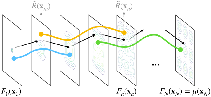
We illustrate the resulting DGFS algorithm in Figure 2. Different from prior works, DGFS can update parameters with incomplete subtrajectories (colored curve segments in the figure) with the help of amortized flow functions, as well as intermediate signals at non-terminal step (grey arrows in the figure), which fundamentally improves the credit assignment process.

Estimation of the partition function.

For an arbitrary trajectory $\tau=\{\mathbf{x}_{n}\}_{n=0}^{N}$, one could define its (log) importance weight to be $S(\tau;{\boldsymbol{\theta}})=\log\mathcal{P}(\mathbf{x}_{0:N})-\log\mathcal{Q}(\mathbf{x}_{0:N};{\boldsymbol{\theta}})$, where $\mathcal{Q}(\mathbf{x}_{0:N};{\boldsymbol{\theta}})=p^{\text{ref}}_{0}(\mathbf{x}_{0})\prod_{n=0}^{N-1}P_{F}(\mathbf{x}_{n+1}|\mathbf{x}_{n};{\boldsymbol{\theta}})$. We obtain the following log-partition function ($\log Z$) estimator:

$$\log\sum_{b=1}^{B}\exp\left(S(\tau^{(b)};{\boldsymbol{\theta}})\right)-\log B\leq\log Z,\quad\tau^{(b)}\sim\mathcal{Q}(\cdot;{\boldsymbol{\theta}}),$$ (17)

where $B\in\mathbb{N}_{+}$ is the number of particles (i.e., trajectories) used for the estimation. Similar to the importance weighted auto-encoders (Burda et al., 2016), our estimator provides a valid lower bound of the logarithm of the normalizing factor with any forward process $\mathcal{Q}$. In this work, we use the difference between estimated log partition function and the ground truth as an evaluation metric. See the Appendix C.2 for additional analysis. We also remark that this approach is similar to the neural importance sampling in Nicoli et al. (2020); Wirnsberger et al. (2020) in the sense that we use the forward process $\mathcal{Q}$ as the proposal distribution.

3.3 Discussion

Variance of gradient updates.

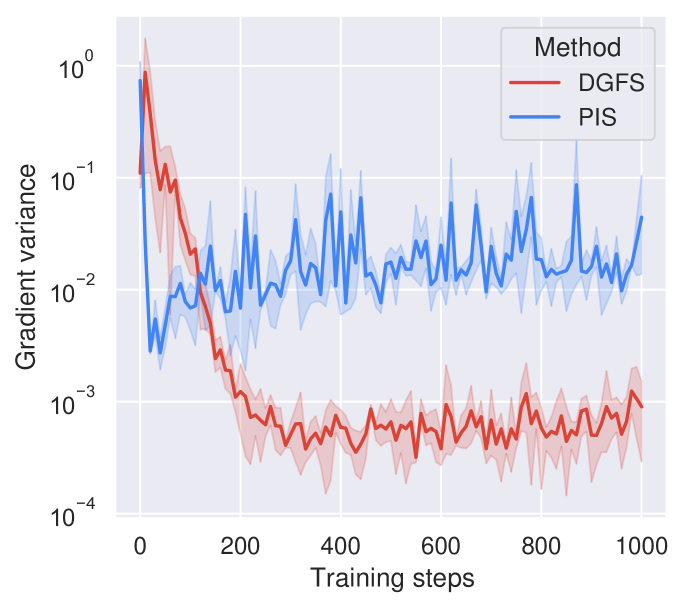
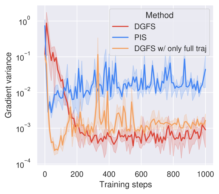
Figure 2 shows that the variance of stochastic gradients with DGFS is much smaller than that with PIS; notice that the comparison is valid as we take the same neural network architecture for both algorithms. We hypothesize that DGFS benefits from the low variance behavior due to the following two reasons: (1) From the perspective of temporal difference learning (Sutton & Barto, 2018; Kearns & Singh, 2000), it has long been discussed that policy learning from shorter trajectory data would lower the variance at the cost of potentially higher bias. Before this work, it was impossible for sampling with stochastic process algorithms to update with partial trajectories, while in the proposed DGFS method, we use an additional flow network to make this feasible. In Figure 4 we also show that the flow network can be properly learned and thus does not introduce much bias, indicating that DGFS achieves a better bias-variance trade-off. (2) Probabilistic ML researchers have shown that for KL divergence based distribution learning, the gradient will not vanish even if the optimal distribution has been reached; see Roeder et al. (2017) and Section 4 of Xu et al. (2022). Later works including Vaitl et al. (2022a; b) propose a different path-gradient estimator to tackle this issue with a similar insight with Roeder et al. (2017); see the related work section. On the other hand, the DGFS objective does achieve zero gradient with the optimal solution (c.f. Appendix C.3), making it a more stable algorithm.

Modeling considerations.

Notice that the DGFS derivation in Section 3 does not rely on the specific form of the stochastic process. Therefore, DGFS could take both the variance exploding (VE) (Zhang & Chen, 2022) or variance preserving (VP) (Vargas et al., 2023a) formulation. In our numerical study, we find the former to be more stable, and thus we default to it unless otherwise specified. We defer related ablations to the Appendix C.5.

Convergence guarantees.

Previous theoretical studies (Bortoli, 2022; Chen et al., 2022; Lee et al., 2022) have demonstrated that the distribution of terminal samples generated by a diffusion model can converge to the target distribution under mild assumptions if the control term is well learned. These findings are also applicable to DGFS since these proofs are independent of how the networks are trained. Additionally, Zhang et al. (2022a) have proven that a perfectly learned score term corresponds to a zero GFlowNet training loss under mild conditions, following theory of GFlowNets (Bengio et al., 2021; 2023). This provides assurance that a sufficiently well-trained DGFS can accurately sample from the target distribution.

4 Related works

Sampling methods.

MCMC methods (Brooks et al., 2011) are the most classical sampling algorithms, with Langevin dynamics (Welling & Teh, 2011) and Hamiltonian Monte Carlo (Duane et al., 1987; Hoffman & Gelman, 2011; Chen et al., 2014) as representatives. With MCMC operators as building blocks, sequential MC methods (Liu, 2001; Doucet et al., 2001) generate samples ancestrally through a series of annealed targets. On the other hand, people turn to parametric models such as deep networks to learn samplers via variational inference (Rezende & Mohamed, 2015). One the most commonly adopted models is the normalizing flow (Dinh et al., 2014) due to its tractability and expressiveness. Various work have been conducted to improve normalizing flow based sampling (Müller et al., 2018; Gao et al., 2020; Wu et al., 2020; Chen et al., 2020; Gabri’e et al., 2021; Arbel et al., 2021; Midgley et al., 2022; de G. Matthews et al., 2022; Caselle et al., 2022). These methods support asymptotically unbiased estimation as shown in Nicoli et al. (2020). What’s more, Vaitl et al. (2022a) propose to to improve the gradient estimation of normalizing flow parameters with the path-gradient technique; Vaitl et al. (2022b) improve continuous normalizing flows based methods (Chen et al., 2018) with a similar technique. These methods have wide applications in natural sciences, for example in lattice field theories (Nicoli et al., 2021; 2023) and targeted free energy estimation (Wirnsberger et al., 2020).

Recently, many researchers have developed powerful diffusion process to model distributions in the generative modeling community (Vincent, 2011; Sohl-Dickstein et al., 2015; Ho et al., 2020a; Song et al., 2020; Du et al., 2022). This inspires people to study how to utilize diffusion process as samplers to learn distribution from given unnormalized target densities (Tzen & Raginsky, 2019; Zhang & Chen, 2022; Vargas et al., 2021; Geffner & Domke, 2022; Doucet et al., 2022; Vargas et al., 2023a; Richter et al., 2023; Vargas & Nusken, 2023; Vargas et al., 2023b). Our work also falls into this category. Specifically, Vargas et al. (2023a) can be seen as a special case of the method proposed in Berner et al. (2022).

GFlowNets.

Table 1: Experimental results on benchmarking target densities. For each algorithm, we report its absolute estimation bias for the log normalizing factor and the corresponding standard deviation. Our method achieves the best performance among the diffusion modeling-based samplers.

	MoG	Funnel	Manywell	VAE	Cox
SMC	$0.289$$\pm 0.112$	$0.307$$\pm 0.076$	$22.36$$\pm 7.536$	$14.34$$\pm 2.604$	$99.61$$\pm 8.382$
VI-NF	$1.354$$\pm 0.473$	$0.272$$\pm 0.048$	$2.677$$\pm 0.016$	$6.961$$\pm 2.501$	$83.49$$\pm 2.434$
CRAFT	$0.348$$\pm 0.210$	$0.454$$\pm 0.485$	$0.987$$\pm 0.599$	$0.521$$\pm 0.239$	$13.79$$\pm 2.351$
FAB w/ Buffer	$0.003$$\pm 0.0005$	$0.0022$$\pm 0.0005$	$0.032$$\pm 0.004$	N/A	$0.19$$\pm 0.04$
PIS	$0.036$$\pm 0.007$	$0.305$$\pm 0.013$	$1.391$$\pm 1.014$	$2.049$$\pm 2.826$	$11.28$$\pm 1.365$
DDS	$0.028$$\pm 0.013$	$0.416$$\pm 0.094$	$1.154$$\pm 0.626$	$1.740$$\pm 1.158$	N/A
DGFS	$0.019$$\pm 0.008$	$0.274$$\pm 0.014$	$0.904$$\pm 0.067$	$0.180$$\pm 0.083$	$8.974$$\pm 1.169$

GFlowNet (Bengio et al., 2023) is a family of generalized variational inference algorithms with a focus on treating the sampling process as a sequential decision-making process. It is original proposed to sample diversity-seeking objects in structured scientific domains such as biological seuqence and molecule design (Bengio et al., 2021; Jain et al., 2022; 2023b; 2023a; Shen et al., 2023; Zhang et al., 2023c; Hernández-García et al., 2023). However, people have developed GFlowNet theories and methodologies to be suitable for generating general objects with composite structures. GFlowNet has rich connection with existing probabilistic ML methods (Zhang et al., 2022b; Zimmermann et al., 2022; Malkin et al., 2023; Zhang et al., 2022a; Hu et al., 2023). Malkin et al. (2023) also show that GFlowNet has the capability of training with off-policy data compared to previous amortized inference methods. As a policy learning framework under Markov decision processes (MDPs), researchers have also drawn fruitful connections between GFlowNet and reinforcement learning (Pan et al., 2023b; c; a). GFlowNet has also been demonstrated to have wide application in causal discovery (Deleu et al., 2022; 2023; Atanackovic et al., 2023), feature attribution (Li et al., 2023a), network structure learning (Liu et al., 2022), job scheduling (Zhang et al., 2023a), and graph combinatorial optimization (Zhang et al., 2023b). Most prior works focus on structured discrete data space. Lahlou et al. (2023) first provides a sound theoretical framework and initial numerical demonstration for using GFlowNet on continuous space. Our work follows this framework and scales up the performance. A prior study (Li et al., 2023b) initially explored GFlowNets in a continuous space, whereas their theory is demonstrated to have non-trivial flaws when considering integration under continuous measure as indicated by Lahlou et al. (2023).

5 Experiments

5.1 Benchmarking target distributions

In this section, we conduct extensive experiments on a diverse set of challenging continuous sampling benchmarks to corroborate the effectiveness of DGFS against previous methods.

Mixture of Gaussians (MoG) is a $2$-dimensional Gaussian mixture where there are $9$ modes designed to be well-separated from each other. The modes share the same variance of $0.3$ and the means are located in the grid of $\{-5,0,5\}\times\{-5,0,5\}$.

Funnel is a classical sampling benchmark problem from Neal (2003); Hoffman & Gelman (2011). This $10$-dimensional density is defined by $\mu(\mathbf{x})=\mathcal{N}(x^{(0)};0,9)\mathcal{N}(\mathbf{x}^{(1:9)};\mathbf{0},\exp(x^{(0)})\mathbf{I})$.

Manywell (Midgley et al., 2022; Noé et al., 2019; Wu et al., 2020) is a $32$-dimensional distribution defined by the product of $16$ same $2$-dimensional “double well” distributions, which share the unnormalized density of $\mu(x,y)=\exp(-x^{4}+6x^{2}+0.5x-0.5y^{2})$.

VAE is a $30$-dimensional sampling task where we use the latent posterior of a pretrained variational autoencoder (Kingma & Welling, 2014; Rezende et al., 2014, VAE) to be the target distribution.

Cox denotes the $1600$-dimensional target distribution of the log Gaussian cox process introduced in Møller et al. (1998) which models the positions of pine saplings. Its unnormalized density is $\mu(\mathbf{x})=\mathcal{N}(\mathbf{x};\mu,\mathbf{K}^{-1})\prod_{d=1}^{D}\exp(x^{(d)}y^{(d)}-\alpha x^{(d)})$, where $\mu,\mathbf{K},\mathbf{y},\alpha$ are constants.

Figure 3: The learned DGFS flow function and the ground truth samples from target process at different diffusion steps. This shows DGFS is able to learn flow functions correctly.

True

PIS

DGFS

DDS

Figure 4: Manywell plots. DGFS and DDS but not PIS recover all modes.

Baselines.

We benchmark DGFS performance against a wide range of strong baseline methods. As an MCMC methods we include the sequential Monte Carlo sampler (Moral & Doucet, 2002, SMC), which is often considered the state-of-the-art sampling method. As for normalizing flow methods we include the variational inference with normalizing flows (Rezende & Mohamed, 2015, VI-NF) approach as well as more recent de G. Matthews et al. (2022, CRAFT) which is combined with MCMC. We also provide results of Midgley et al. (2022, FAB) with a replay buffer that utilizes the annealed importance sampling technique to augment the training. Last but not least, we compare with PIS (Zhang & Chen, 2022) and DDS (Vargas et al., 2023a) algorithms which are closest to our framework but trained with the KL divergence formulation (Equation 5) without the improved training techniques described in Section 3.

Evaluation protocol.

We measure the performance of different algorithms by their estimation bias of the log normalizing factor of unnormalized target distributions. Contrary to Zhang & Chen (2022) which take the best checkpoint across the run, in this work we compute the average of the last ten checkpoints for a more robust comparison. All results are conducted with $5$ random seeds.

We display the benchmarking results in Table 1. We fail to achieve reasonable performance with DDS on Cox target where we mark it as “N/A”. The advantage of the proposed DGFS method can be observed across different tasks, indicating it could indeed benefit from its design providing more informative training signals to achieve better convergence and capturing diverse modes even in high dimensional spaces. FAB with buffer produces highly stable results, which can be attributed to both annealed importance sampling, the use of buffers, larger networks, and other tricks. It is also remarkable that DGFS obtains very stable results compared to other baselines with diffusion modeling (PIS, DDS). We defer related experimental details and extra experiments to Appendix C.

5.2 Analysis

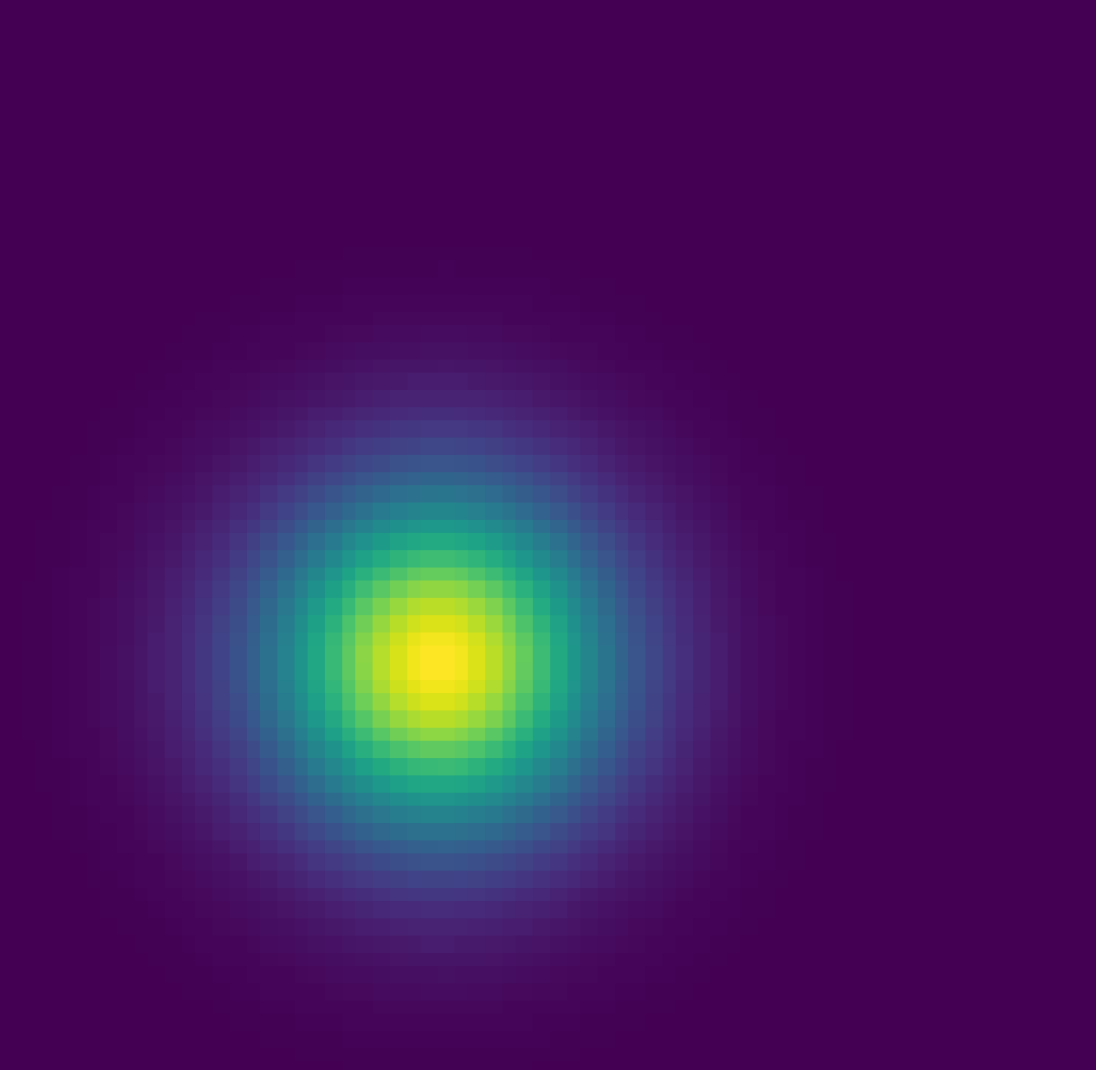
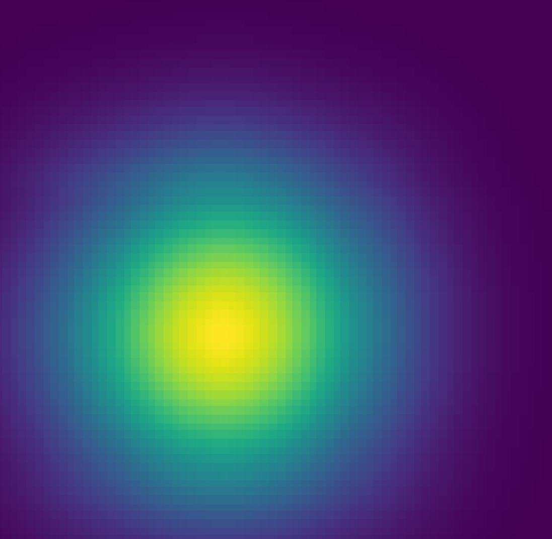
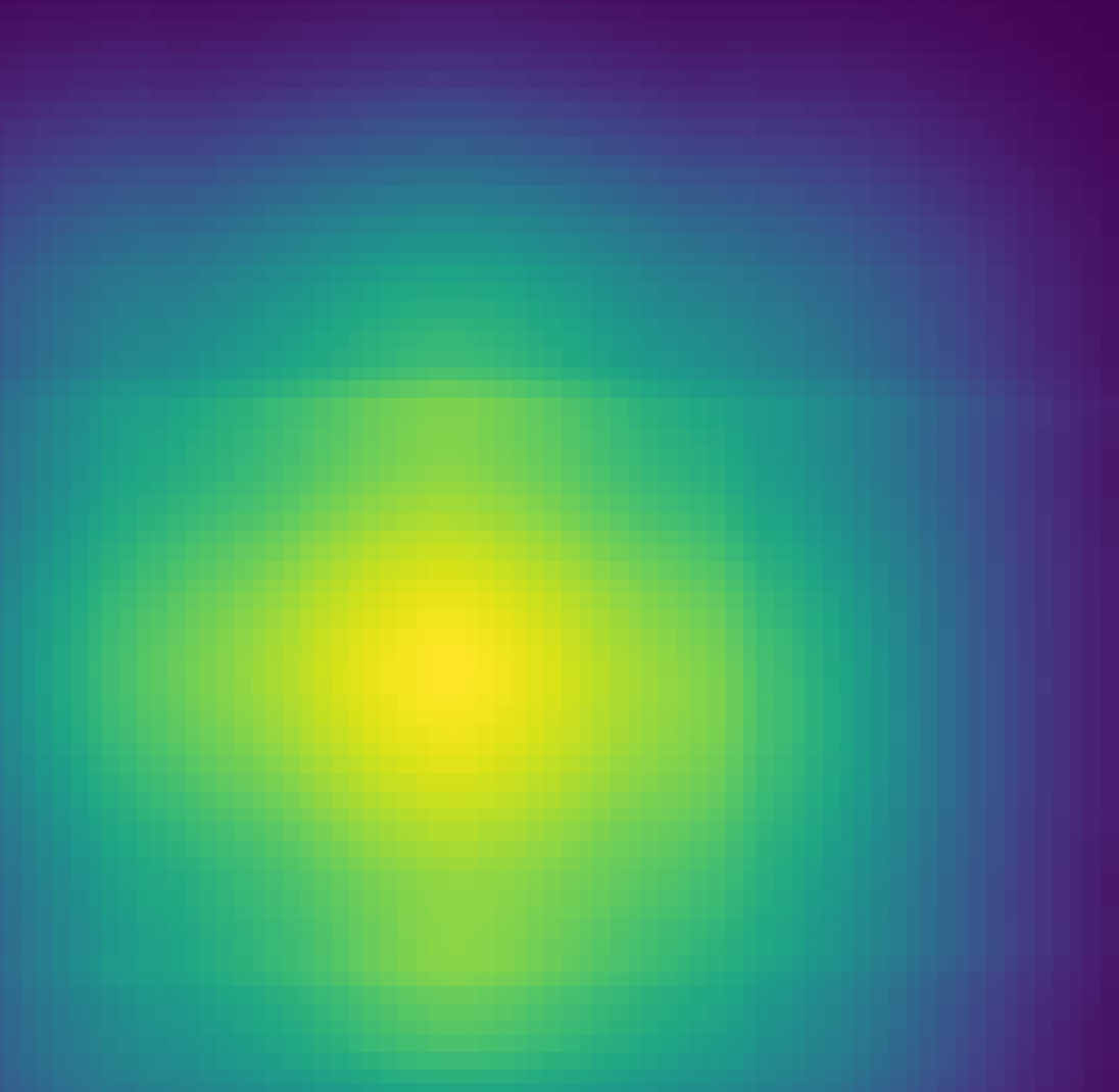
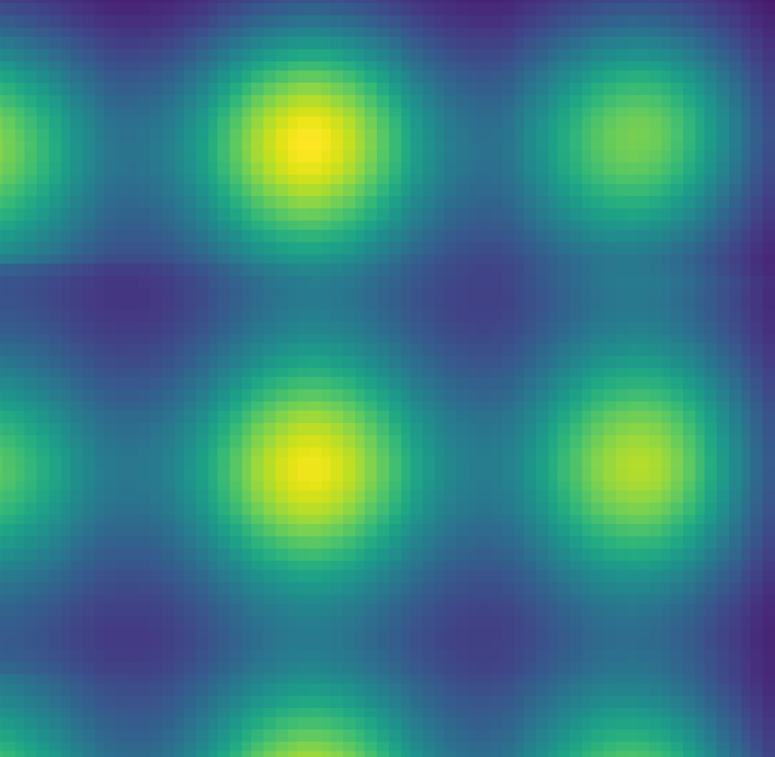
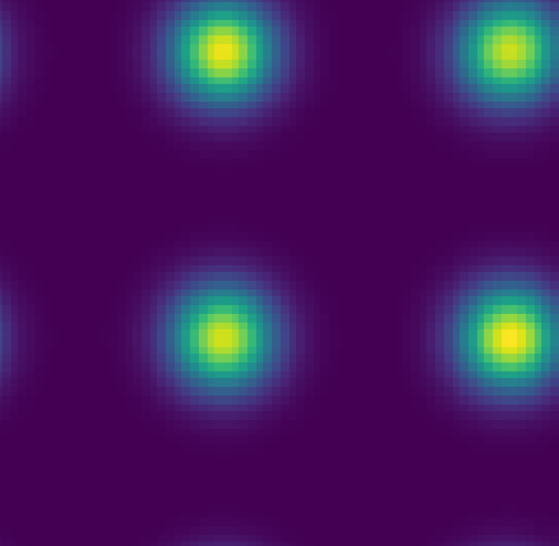
First, we investigate the learning of the flow function introduced in Equation 12. In the first row of Figure 4, we visualize the learned flow function $F_{n}(\mathbf{x}_{n})$ with $n=20,40,\ldots,100$ in the $2$D MoG task. In the second row, we simulate samples from $p_{n}(\mathbf{x}_{n})$ by sampling according to Equation 11, i.e., moving ground truth $\pi(\cdot)$ samples in the backward direction with policy $P_{B}$. The consistency between these two rows indicate that DGFS flow function can successfully approximate the intermediate marginal $p_{n}(\cdot)$, which makes it possible to provide an effective training signal for learning from partial trajectory pieces.

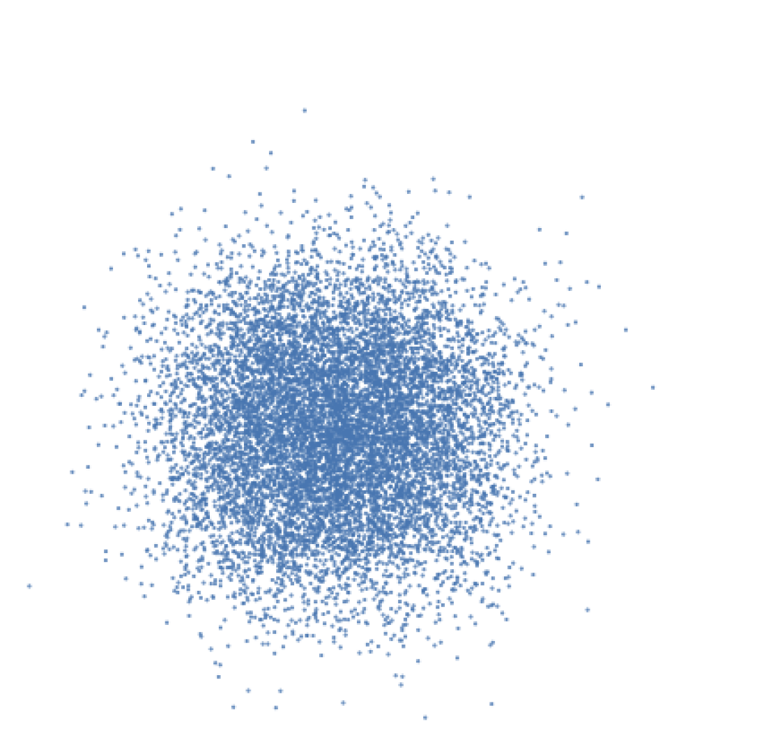
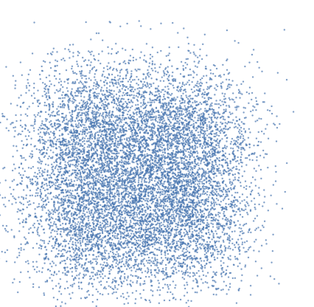
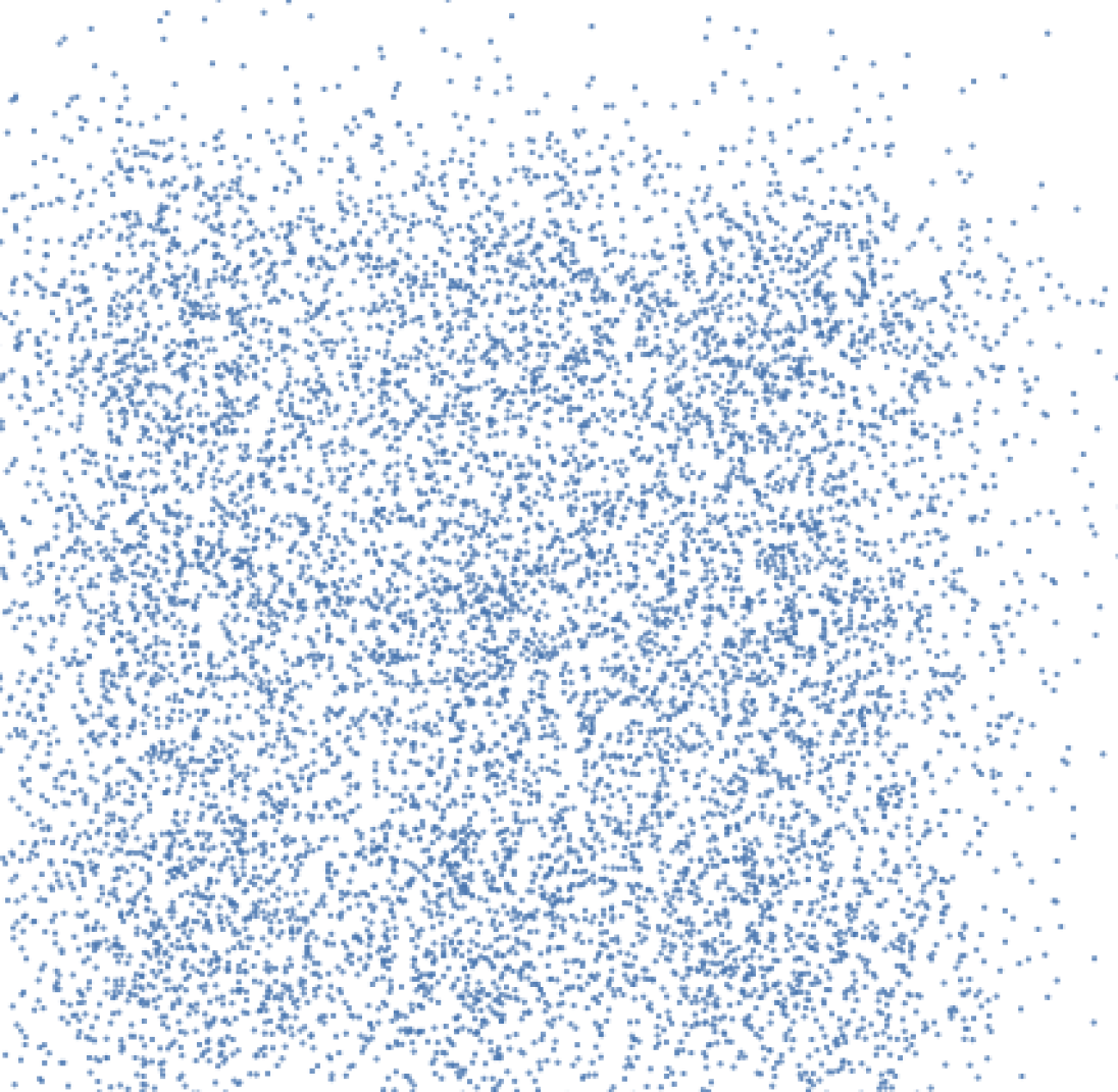
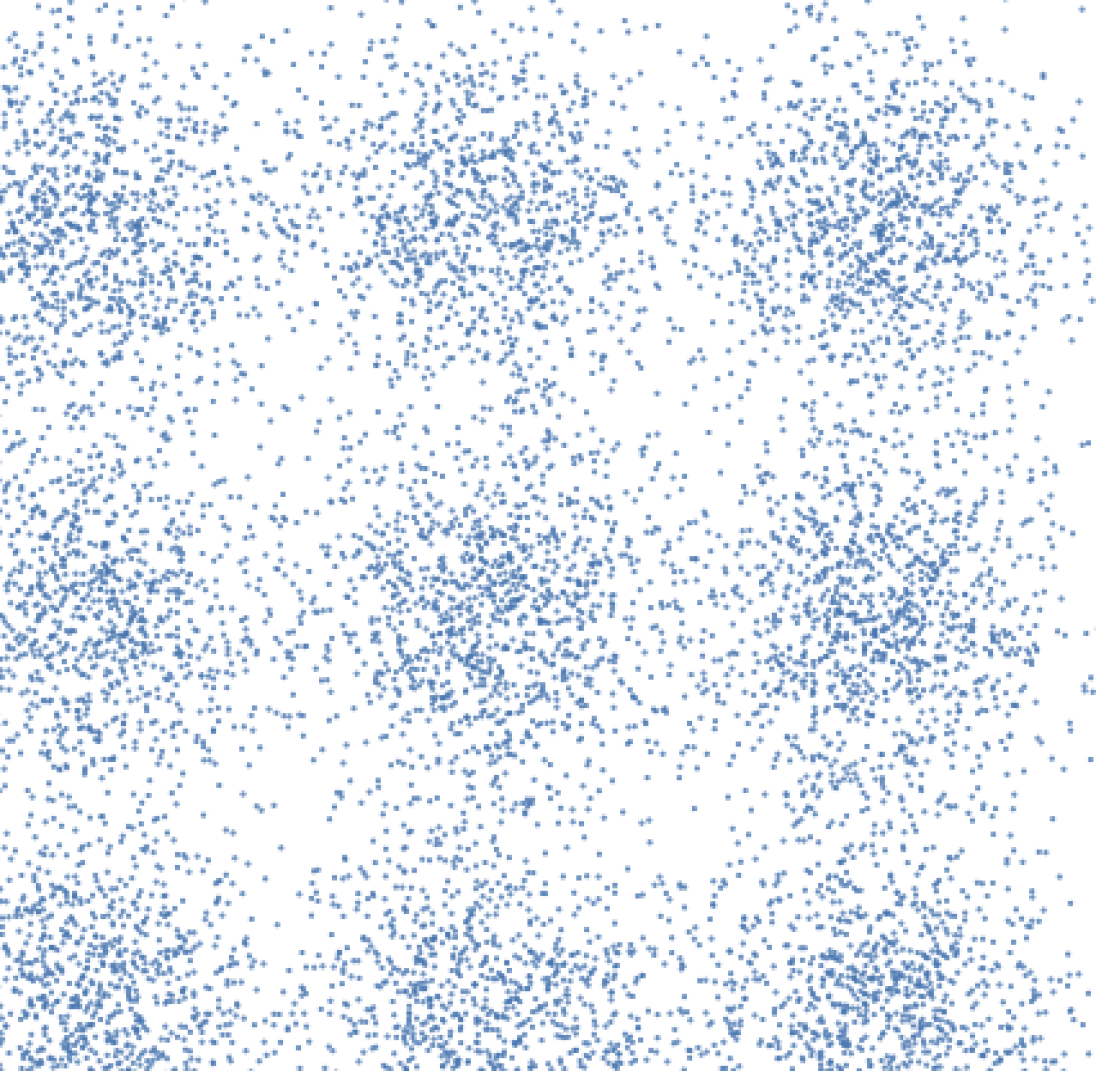
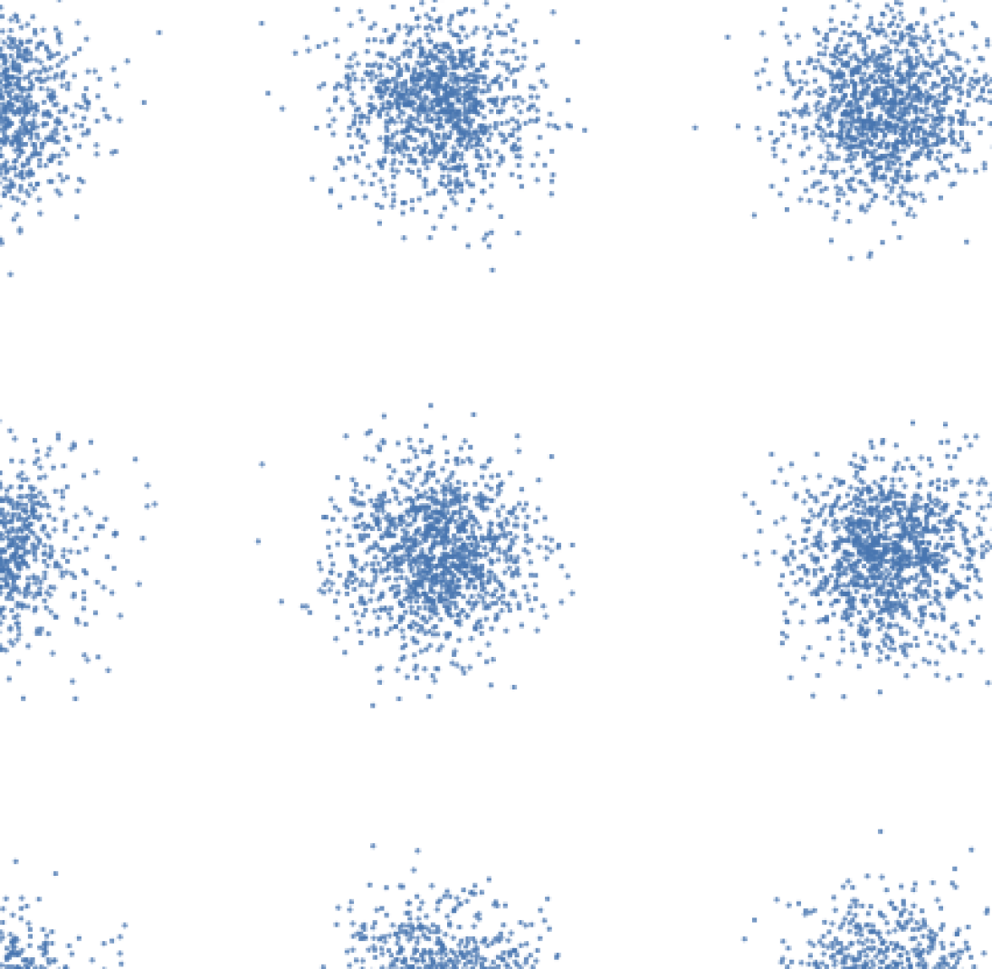
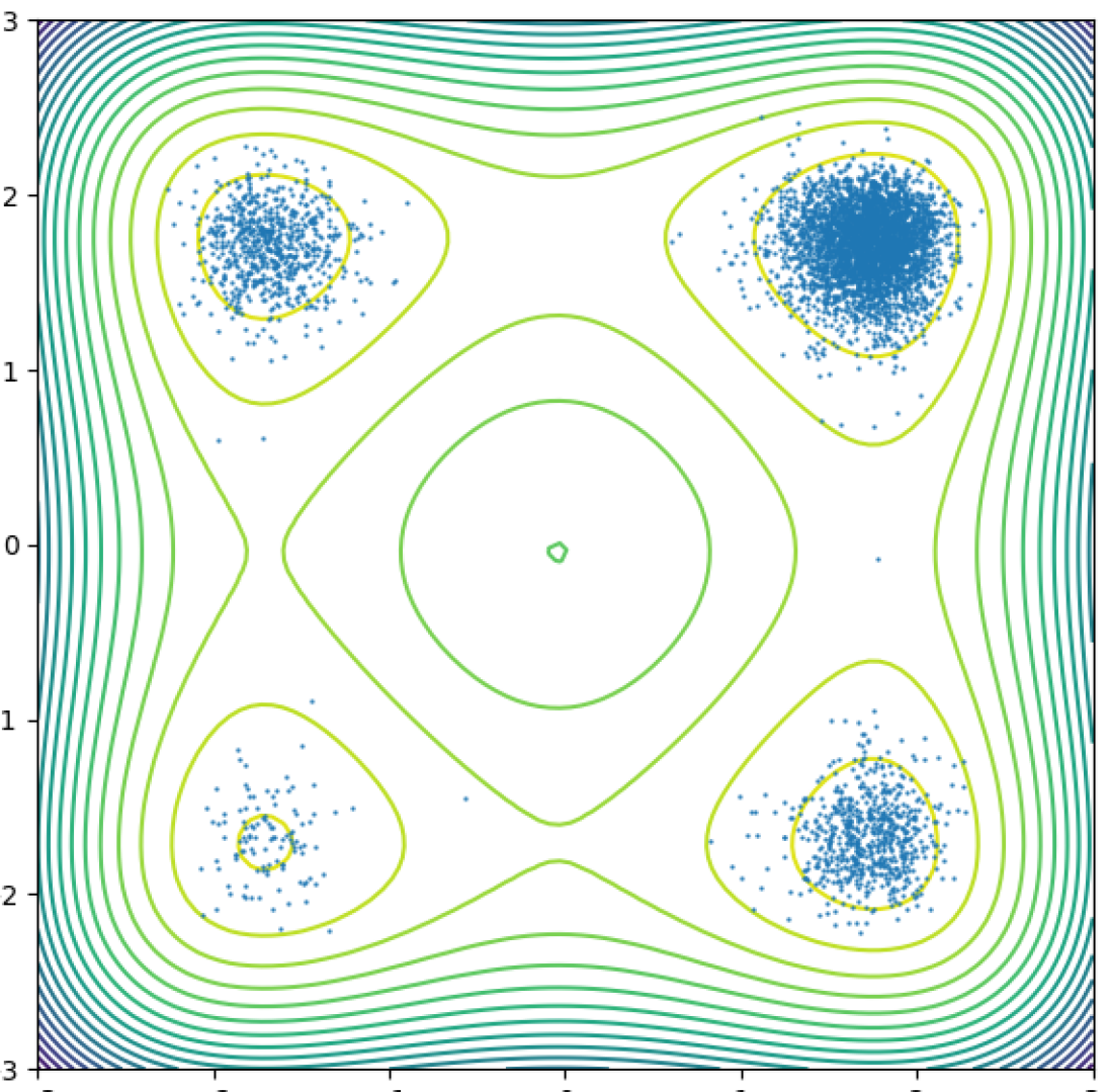
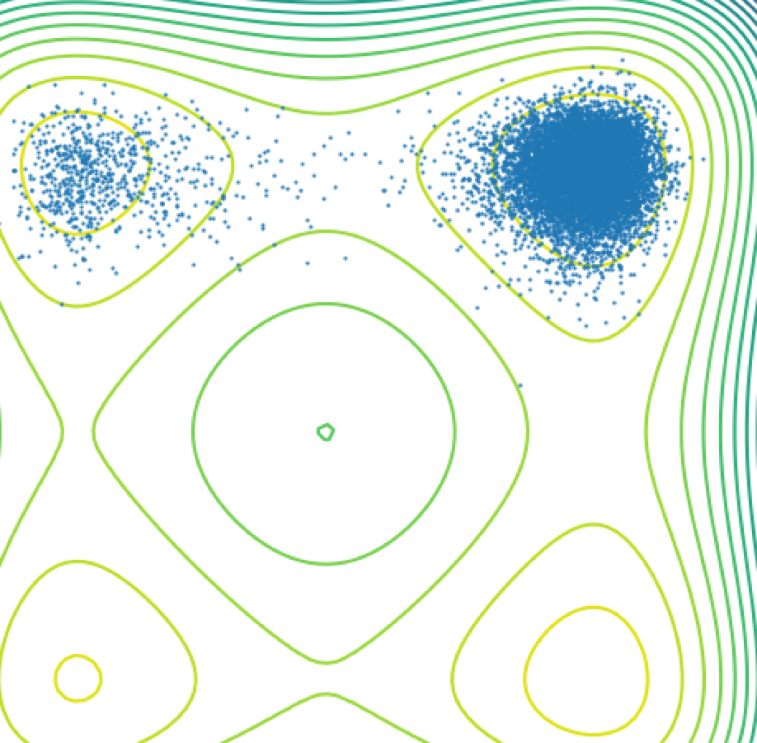
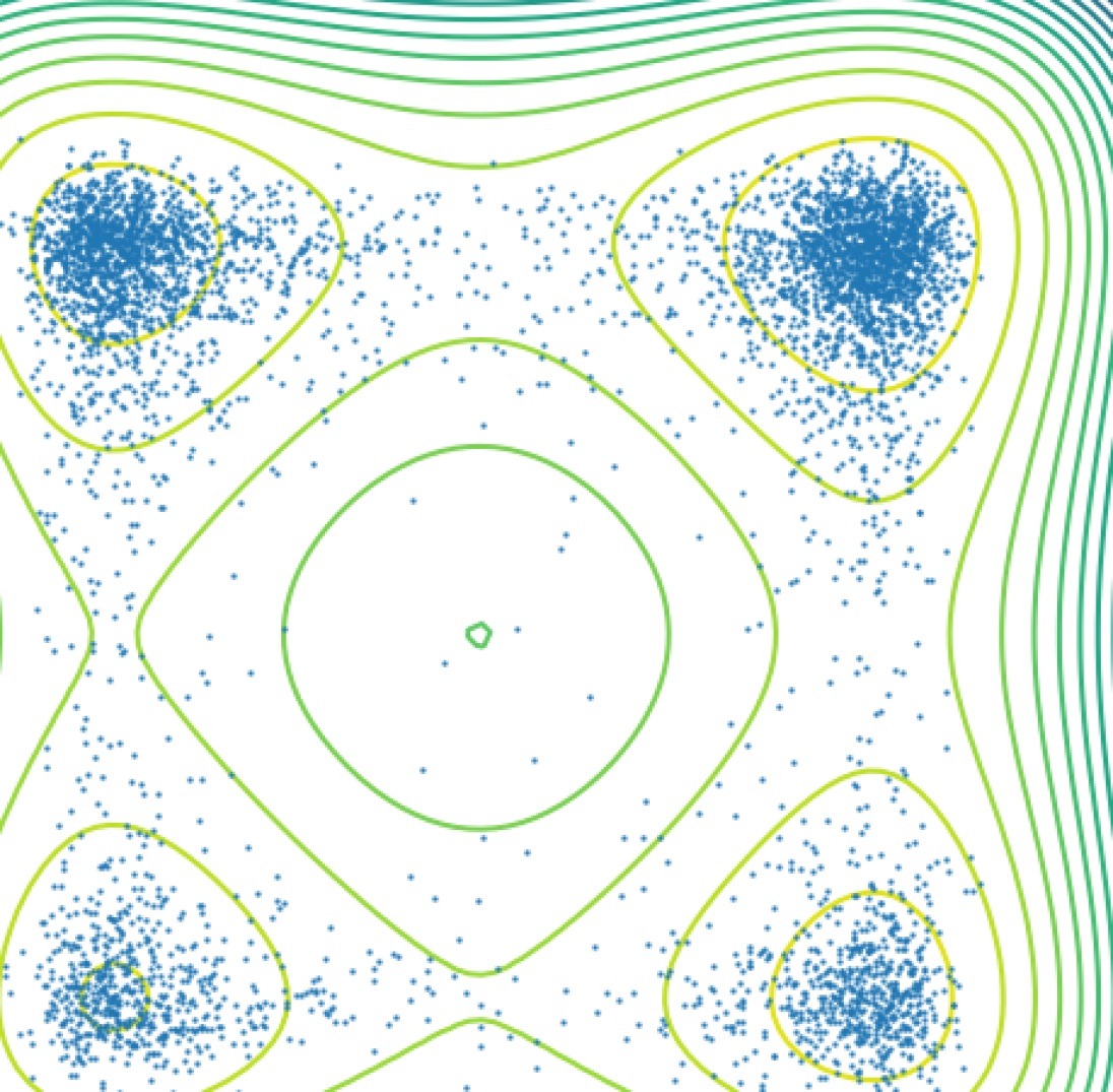
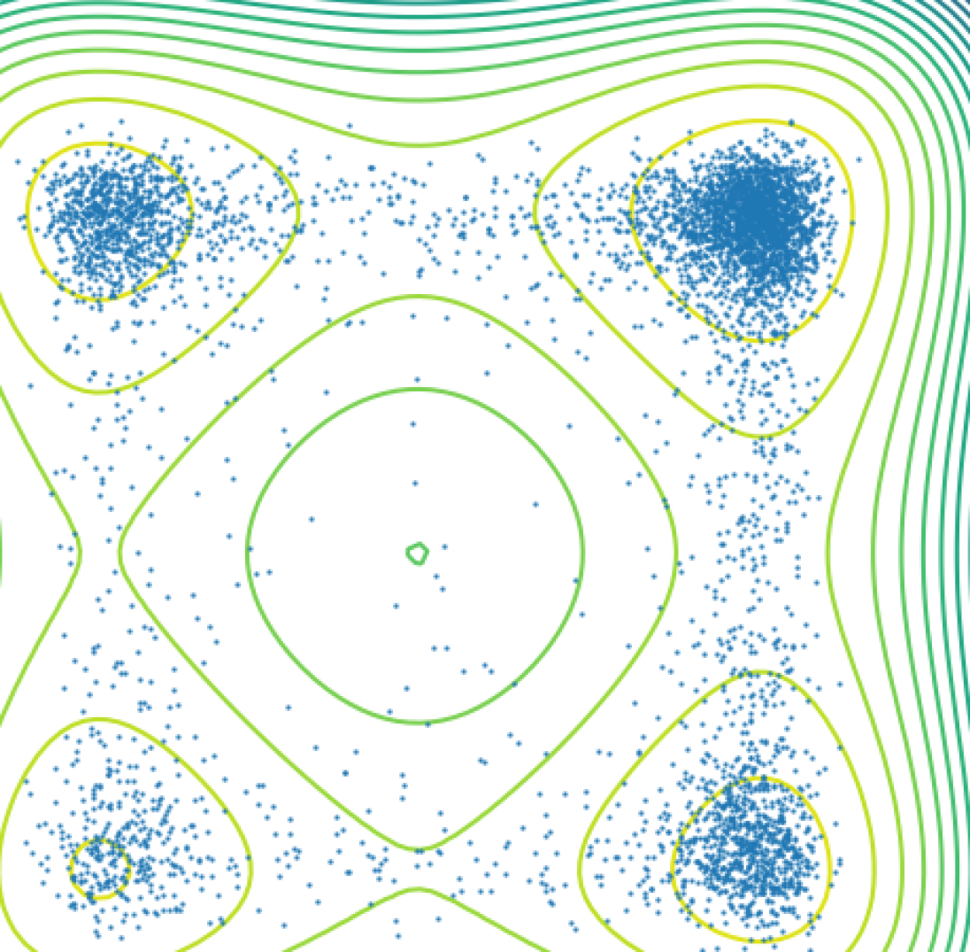
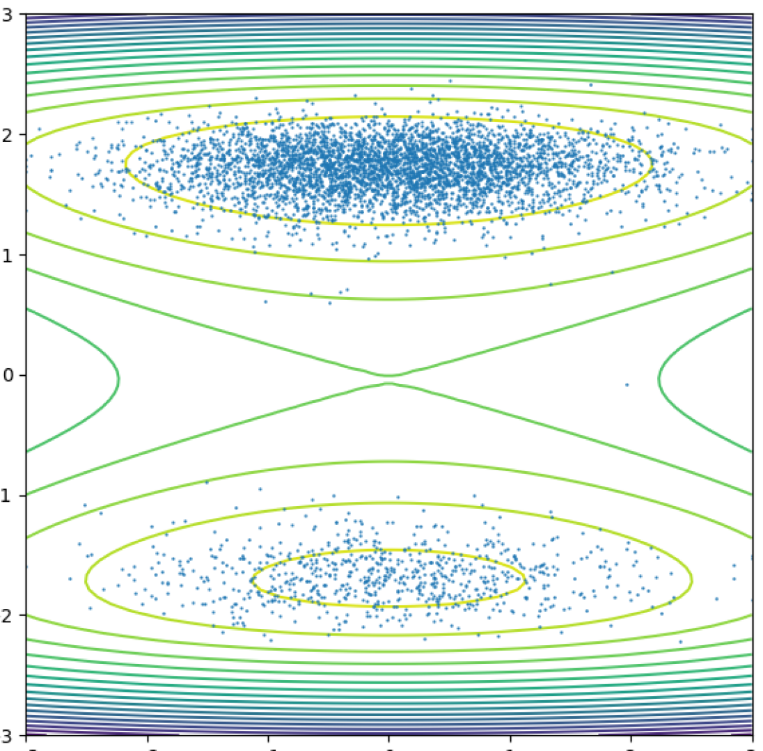
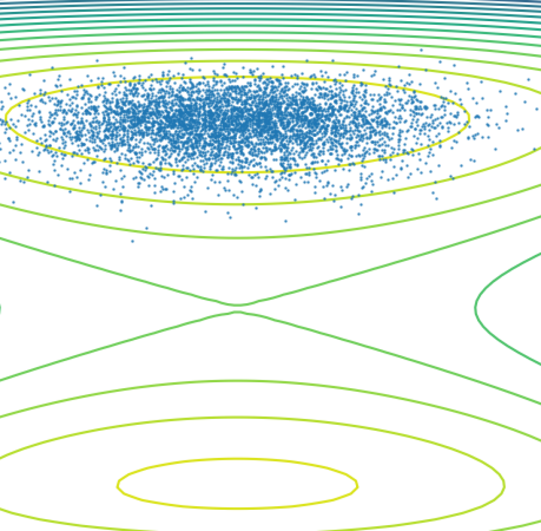
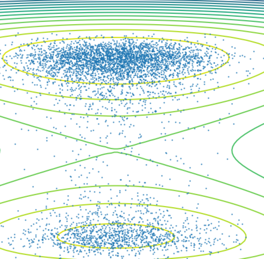
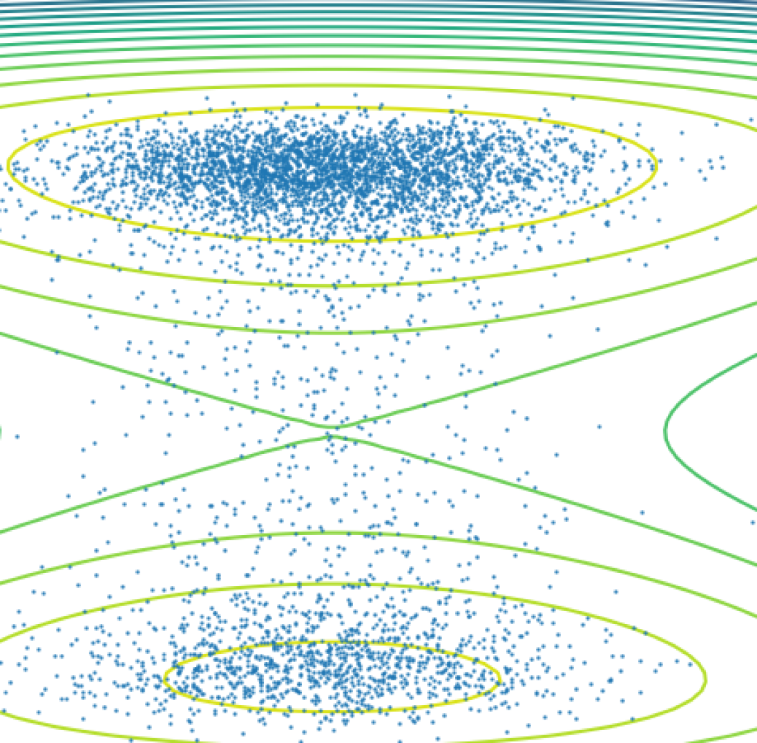
For the MoG task, we demonstrate the samples together with ground truth contours in Figure 5. This visualization result matches the log partition function estimation bias in Table 1, where DGFS generates the nine modes more uniformly than other baselines. This corroborates the advantage of DGFS to capture all different modes in a complex landscape. We then show visualization results on the Manywell task in Figure 4. The Manywell distribution is $32$-dimensional, so we display the joint of the first and third dimension. We plot the samples generated from the true distribution and different algorithms, together with the true density contours. This figure implies that PIS can model half of the modes in these two dimensions well, but miss the other two modes, whereas both DGFS and DDS could cover all four modes. Further, DGFS achieves slightly better mode capturing than DDS in the sense that its modes are more separate and thus closer to the true distribution, while for DDS there are considerable samples appear between the upper right mode and the bottom right mode, which is not ideal. We defer other visualizations to the Appendix C.5.

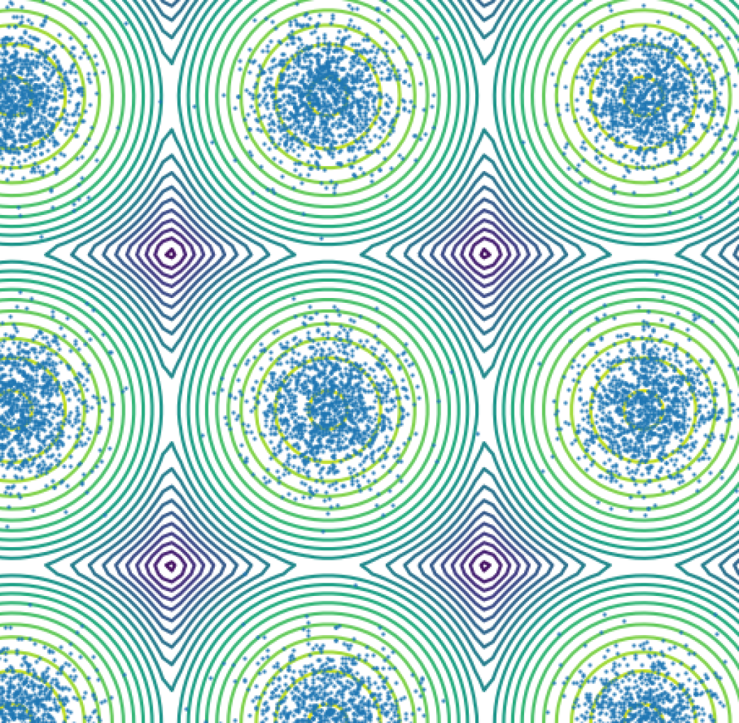
DGFS

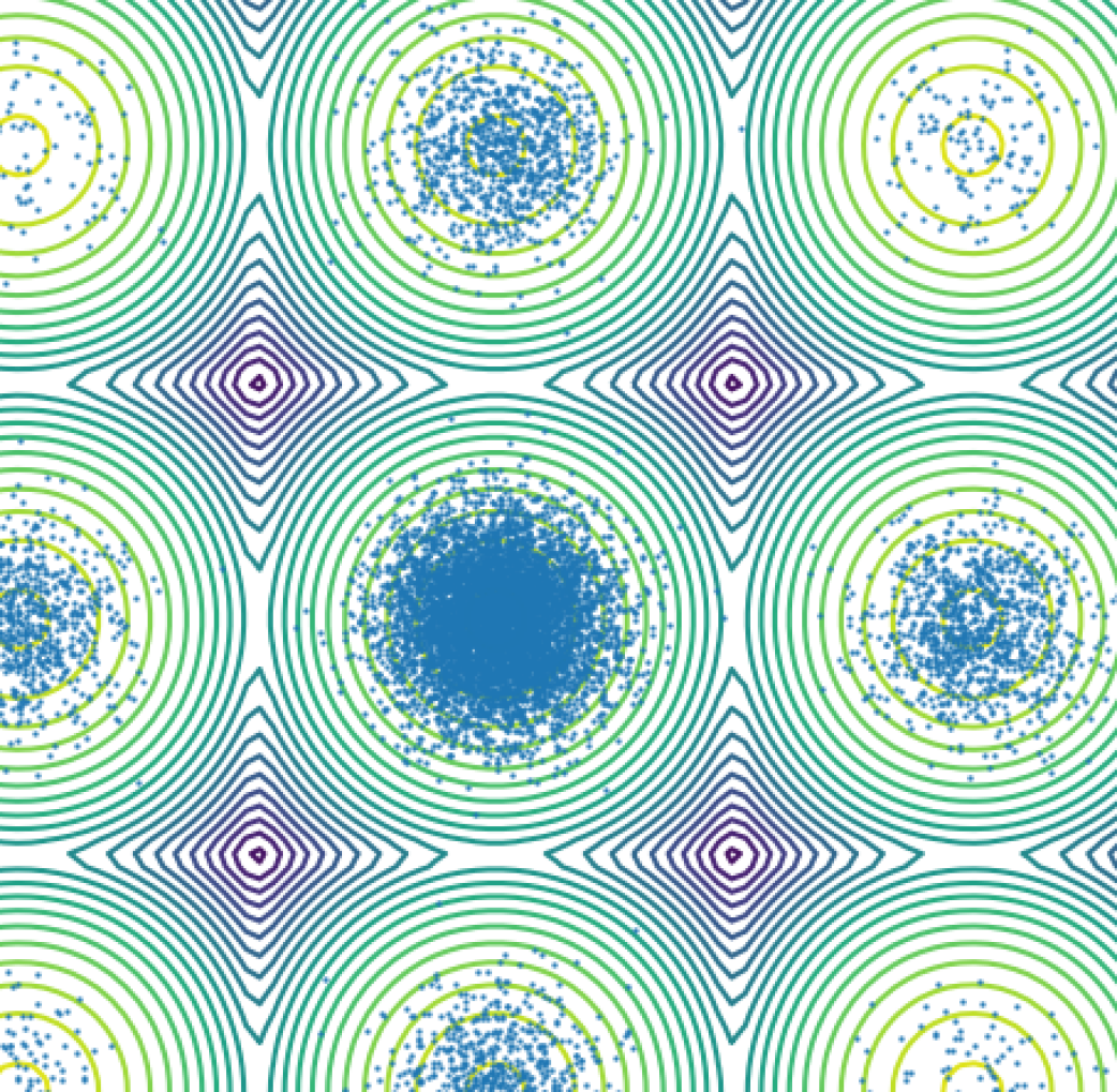
PIS

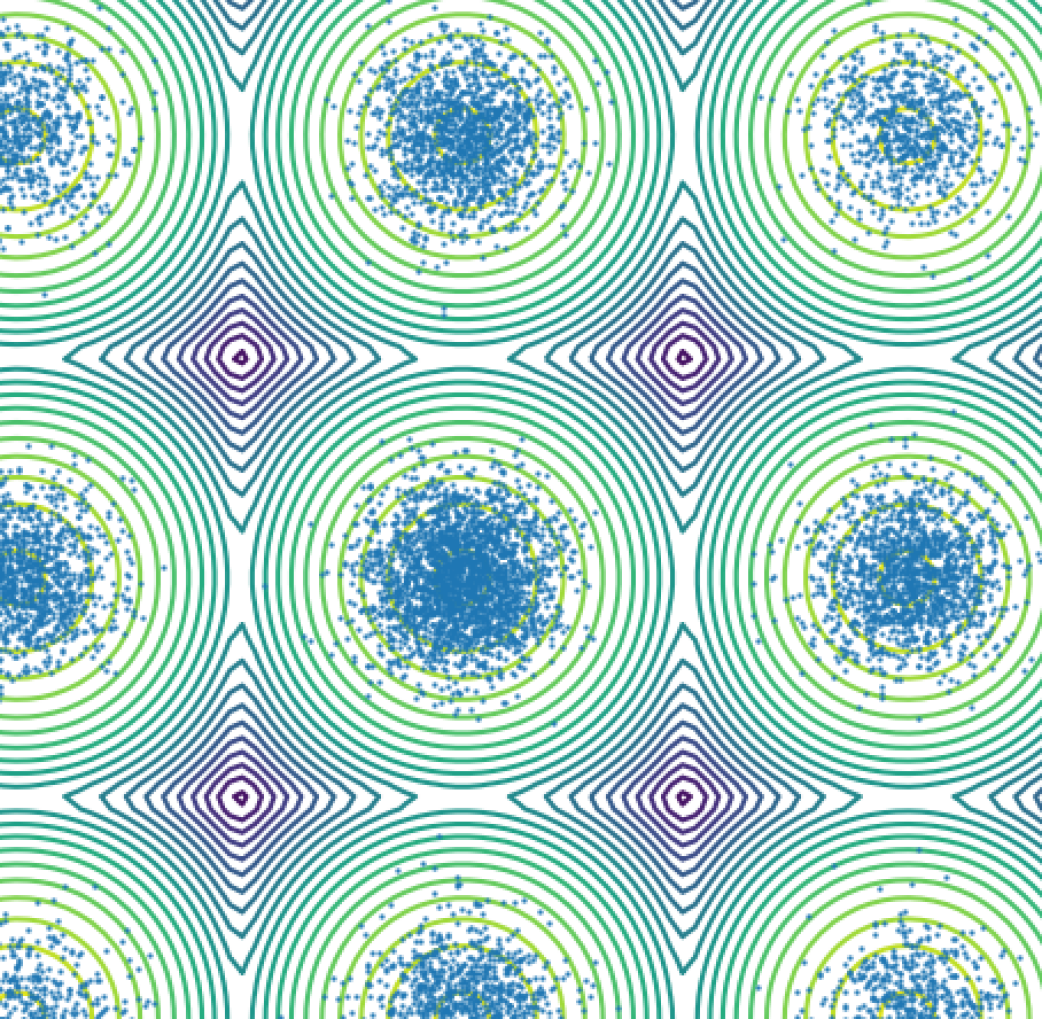
DDS

Figure 5: MoG visualization of DGFS and other diffusion-based samplers shows that DGFS could capture the diverse modes well, better than PIS and DDS. The contours display the landscape of the target density.

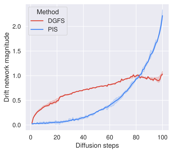
To look into why DGFS outperforms PIS with similar architecture, we plot the learned drift network magnitude in Figure 8 in the Appendix. The result shows that the solution that DGFS achieved has more homogeneous magnitude outputs across different diffusion steps. This may explain one reason why DGFS is easier to train than PIS, since the policy probabilities at different steps $\{P_{F}(\cdot|\mathbf{x}_{n})\}_{n}$ are actually parameterized by a single neural network with temporal embedding input. This makes the learning task more stationary with DGFS. We also conduct in-depth ablation studies to evaluate the design choices of DGFS in Appendix C.5 and C.7.

6 Conclusion

We propose the Diffusion Generative Flow Sampler (DGFS), a novel algorithm that trains diffusion models to sample from given unnormalized target densities. Different from prior works that could only learn from complete diffusion chains, DGFS could update its parameter with only partial specification of the stochastic process trajectory; what’s more, DGFS can receive intermediate signals before completing the entire path. These features help DGFS benefit from efficient credit assignment and thus achieve better partition function estimation bias in the sampling benchmarks.

The DGFS framework presents various opportunities for further research, fueled by its inherent limitations. To name a few, how can we better design the intermediate local signals in ways more sophisticated than the current straightforward approach? Additionally, can we harness DGFS’s exploration capabilities to succeed in high dimensional tasks, pushing the boundaries of its performance? Can we combine DGFS with a prioritized replay buffer? This would largely reduce the number of querying $\mu(\cdot)$. From the perspective of application, there are also many interesting research questions. Can we deploy DGFS on scientific biological or chemical tasks such as protein conformation modeling? Can we incorporate equivariance into the modeling of DGFS to increase efficiency? We expect that exploring these future directions will lead to valuable insights and bring fruit follow-ups of DGFS.

Ethics Statement

We commit to the ICLR Code of Ethics and affirm that our work only utilizes public datasets for experimentation. While our empirical results are largely based on synthetic data, we acknowledge the potential for misuse and urge the responsible application of the proposed methods with real-world data. We welcome any related discussions and feedback.

Reproducibility statement

We provide detailed algorithmic and experimental description in Section 3 and Appendix C, and we have attached the complete code accompanying this research. To ensure robustness and reliability of our empirical results, every experiment conducted was replicated using five distinct random seeds. Upon publication, the codebase will be released on Github.

Appendix A Notations

Symbol	Description
$\mathbb{R}^{D}$	$D$-dimensional real space
$N\in\mathbb{N}_{+}$	number of steps in the discrete-time stochastic process
$\mathcal{S}$	GFlowNet state space, equals $\{(n,\mathbf{x}_{n}):n\in\{0,1,\ldots,N\},\mathbf{x}_{n}\in\mathbb{R}^{D}\}$;
	$(n,\mathbf{x}_{n})$ is often writen as $\mathbf{x}_{n}$ for simplicity
$\mathcal{A}$	action / transition space (edges $\mathbf{s}\to\mathbf{s}^{\prime}$)
$\mathbf{s}$	state in $\mathcal{S}$
$\mathbf{s}_{0}$	initial state, equals $(0,\mathbf{0})$ in VE modeling
$\tau$	complete trajectory $(\mathbf{x}_{0}\to\ldots\to\mathbf{x}_{N})$, or $\mathbf{x}_{0:N}$
${\boldsymbol{\theta}}$	learnable parameter of DGFS
$F_{n}:\mathbb{R}^{D}\to\mathbb{R}_{+}$	state flow function at step $n$
$P_{F}$	forward policy (distribution over children / next step)
$P_{B}$	backward policy (distribution over parents / previous step)
$\mathcal{Q}$	forward process defined in Equation 1
$\mathcal{Q}^{\text{ref}}$	reference process defined in Equation 3
$\mathcal{P}$	target process defined in Equation 4
$p^{\text{ref}}_{n}:\mathbb{R}^{D}\to\mathbb{R}_{+}$	marginal distribution of reference process at step $n$
$h\in\mathbb{R}_{+}$	discretized step size for the stochastic process
$\mathbf{f}$	drift term in the VE stochastic process (Equation 5)
$\sigma$	variance coefficient in the stochastic process
$\mathop{}\!\mathrm{d}\mathbf{W}_{t}$	standard Wiener process in continuous-time stochastic process
$R:\mathbb{R}^{D}\to\mathbb{R}_{+}$	reward function (unnormalized target density)
$\tilde{R}_{n}:\mathbb{R}^{D}\to\mathbb{R}_{+}$	intermediate forward-looking signal defined in Equation 16
$Z\in\mathbb{R}_{+}$	scalar, equal to $\sum_{\mathbf{x}\in\mathbb{R}^{D}}R(\mathbf{x})$
$\mu:\mathbb{R}^{D}\to\mathbb{R}_{+}$	same thing as $R(\cdot)$
$\pi:\mathbb{R}^{D}\to\mathbb{R}_{+}$	normalized density, equal to $\mu(\cdot)/Z$

Appendix B Details about stochastic processes

B.1 Variance exploding (VE) process

Song et al. (2020) and Zhang & Chen (2022) take a variance exploding stochastic process modeling. In Zhang & Chen (2022), the authors use Gisarnov theorem to derive an optimal control objective for KL divergence minimization. In this work, we present a discrete-time derivation for completeness.

The reference process starts at $p^{\text{ref}}_{0}(\cdot)$, which is a Dirac distribution at $\mathbf{0}$, and writes

$$\mathcal{Q}^{\text{ref}}(\mathbf{x}_{0:N}) :\;\mathbf{x}_{n+1}=\mathbf{x}_{n}+\sqrt{h}\sigma{\boldsymbol{\epsilon}}_{n},{\boldsymbol{\epsilon}}_{n}\sim\mathcal{N}(\mathbf{0},\mathbf{I}),\mathbf{x}_{0}=\mathbf{0},$$ (18)

$$\Rightarrow\mathcal{Q}^{\text{ref}}(\mathbf{x}_{0:N}) =p^{\text{ref}}_{0}(\mathbf{x}_{0})\prod_{n=0}^{N-1}P_{F}^{\text{ref}}(\mathbf{x}_{n+1}|\mathbf{x}_{n})=p^{\text{ref}}_{N}(\mathbf{x}_{N})\prod_{n=0}^{N-1}P_{B}(\mathbf{x}_{n}|\mathbf{x}_{n+1}).$$ (19)

Therefore, $p_{n}^{\text{ref}}(\cdot)=\mathcal{N}(\cdot;\mathbf{0},hn\sigma^{2}\mathbf{I})$. According to Bayesian formula,

$$P_{B}(\mathbf{x}_{n}|\mathbf{x}_{n+1}) =\frac{p_{n}^{\text{ref}}(\mathbf{x}_{n})P_{F}^{\text{ref}}(\mathbf{x}_{n+1}|\mathbf{x}_{n})}{p_{n+1}^{\text{ref}}(\mathbf{x}_{n+1})}=\frac{\mathcal{N}(\mathbf{x}_{n};\mathbf{0},hn\sigma^{2}\mathbf{I})\mathcal{N}(\mathbf{x}_{n+1};\mathbf{x}_{n},h\sigma^{2}\mathbf{I})}{\mathcal{N}(\mathbf{x}_{n+1};\mathbf{0},h(n+1)\sigma^{2}\mathbf{I})}$$ (20)

$$=\mathcal{N}(\mathbf{x}_{n};\frac{n}{n+1}\mathbf{x}_{n+1},\frac{n}{n+1}h\sigma^{2}\mathbf{I}).$$ (21)

The target process is then

$$\mathcal{P}(\mathbf{x}_{0},\ldots,\mathbf{x}_{N})=\mathcal{Q}^{\text{ref}}(\mathbf{x}_{0},\ldots,\mathbf{x}_{N})\frac{\pi(\mathbf{x}_{N})}{p_{N}^{\text{ref}}(\mathbf{x}_{N})}=\pi(\mathbf{x}_{N})\prod_{n=0}^{N-1}P_{B}(\mathbf{x}_{n}|\mathbf{x}_{n+1}).$$ (22)

The trajectory level log probability difference between model and target is

$$\log\frac{\mathcal{Q}}{\mathcal{P}}=\log\frac{\mathcal{Q}}{\mathcal{Q}^{\text{ref}}}+\log\frac{\mathcal{Q}^{\text{ref}}}{\mathcal{P}}.$$ (23)

It is obvious that the second term is $\frac{\mathcal{Q}^{\text{ref}}}{\mathcal{P}}=\frac{p_{N}^{\text{ref}}(\mathbf{x}_{N})}{\pi(\mathbf{x}_{N})}$, thus we only need to look at the first term

$$\log\frac{\mathcal{Q}}{\mathcal{Q}^{\text{ref}}} =\sum_{n=0}^{N-1}\log\frac{P_{F}(\mathbf{x}_{n+1}|\mathbf{x}_{n};{\boldsymbol{\theta}})}{P_{F}^{\text{ref}}(\mathbf{x}_{n+1}|\mathbf{x}_{n})}=\sum_{n=0}^{N-1}\log\frac{\mathcal{N}(\cdot;\mathbf{x}_{n}+h\mathbf{f}(\mathbf{x}_{n},n),h\sigma^{2}\mathbf{I})}{\mathcal{N}(\cdot;\mathbf{x}_{n},h\sigma^{2}\mathbf{I})}$$ (24)

$$=\sum_{n=0}^{N-1}\left(\frac{h}{2\sigma^{2}}\|\mathbf{f}(\mathbf{x}_{n},n;{\boldsymbol{\theta}})\|^{2}+\frac{\sqrt{h}}{\sigma^{2}}\mathbf{f}(\mathbf{x}_{n},n;{\boldsymbol{\theta}})^{T}{\boldsymbol{\epsilon}}_{n}\right).$$ (25)

Notice that under the expectation of $\mathcal{Q}$,

$$\mathbb{E}_{\mathcal{Q}}\left[\mathbf{f}(\mathbf{x}_{n},n;{\boldsymbol{\theta}})^{T}{\boldsymbol{\epsilon}}_{n}\right]=\mathbf{f}(\mathbf{x}_{n},n;{\boldsymbol{\theta}})^{T}\mathbb{E}_{\mathcal{Q}}\left[{\boldsymbol{\epsilon}}_{n}\right]=0.$$ (26)

Accordingly,

$$\mathcal{D}_{\mathrm{KL}}\left(\mathcal{Q}\|\mathcal{P}\right)=E_{\mathcal{Q}}\left[\log\frac{\mathcal{Q}}{\mathcal{P}}\right]=E_{\mathcal{Q}}\left[\sum_{n=0}^{N-1}\frac{h}{2\sigma^{2}}\|\mathbf{f}(\mathbf{x}_{n},n;{\boldsymbol{\theta}})\|^{2}+\log\frac{p_{N}^{\text{ref}}(\mathbf{x}_{N})}{\pi(\mathbf{x}_{N})}\right],$$ (27)

which leads us to Equation 6.

B.2 Variance preserving (VP) process

Ho et al. (2020b) and Vargas et al. (2023a) take this VP formulation of diffusion process. The derivation is similar to the last section, just with a different variance schedule.

We first define the backward policy

$$P_{B}(\mathbf{x}_{n}|\mathbf{x}_{n+1})=\mathcal{N}(\mathbf{x}_{n};\sqrt{1-\beta_{n}}\mathbf{x}_{n+1};\beta_{n}\sigma^{2}\mathbf{I}).$$ (28)

Then The target and reference process are

$$\mathcal{P}(\mathbf{x}_{0:N}) =\pi(\mathbf{x}_{N})\prod_{n=0}^{N-1}P_{B}(\mathbf{x}_{n}|\mathbf{x}_{n+1}),$$ (29)

$$\mathcal{Q}^{\text{ref}}(\mathbf{x}_{0:N}) =p^{\text{ref}}_{N}(\mathbf{x}_{N})\prod_{n=0}^{N-1}P_{B}(\mathbf{x}_{n}|\mathbf{x}_{n+1}),$$ (30)

where $p^{\text{ref}}_{N}(\cdot)=\mathcal{N}(\cdot;\mathbf{0},\sigma^{2}\mathbf{I})$. This guarantees that $p^{\text{ref}}_{n}(\cdot)=\mathcal{N}(\cdot;\mathbf{0},\sigma^{2}\mathbf{I}),\forall n$.

From using Bayesian formula on $\mathcal{Q}^{\text{ref}}$,

$$P_{F}^{\text{ref}}(\mathbf{x}_{n+1}|\mathbf{x}_{n})=\frac{p^{\text{ref}}_{n+1}(\mathbf{x}_{n+1})P_{B}(\mathbf{x}_{n}|\mathbf{x}_{n+1})}{p^{\text{ref}}_{n}(\mathbf{x}_{n})}=\mathcal{N}(\mathbf{x}_{n+1};\sqrt{1-\beta_{n}}\mathbf{x}_{n},\beta_{n}\sigma^{2}\mathbf{I}).$$ (31)

Inspired by this, let us define the (learnable) forward process to be

$$P_{F}(\mathbf{x}_{n+1}|\mathbf{x}_{n};{\boldsymbol{\theta}}) =\mathcal{N}(\mathbf{x}_{n+1};\sqrt{1-\beta_{n}}\mathbf{x}_{n}+\mathbf{f}(\mathbf{x}_{n},n;{\boldsymbol{\theta}}),\beta_{n}\sigma^{2}\mathbf{I}),$$ (32)

$$\mathcal{Q}(\mathbf{x}_{0:N}) =p^{\text{ref}}_{0}(\mathbf{x}_{0})\prod_{n=0}^{N-1}P_{F}(\mathbf{x}_{n+1}|\mathbf{x}_{n};{\boldsymbol{\theta}}).$$ (33)

Similar to the derivation in VE,

$$\mathbb{E}_{\mathcal{Q}}\left[\log\frac{\mathcal{Q}}{\mathcal{Q}^{\text{ref}}}\right] =\mathbb{E}_{\mathcal{Q}}\left[\sum_{n=0}^{N-1}\log\frac{P_{F}(\mathbf{x}_{n+1}|\mathbf{x}_{n};{\boldsymbol{\theta}})}{P_{F}^{\text{ref}}(\mathbf{x}_{n+1}|\mathbf{x}_{n})}\right]=\sum_{n=0}^{N-1}E_{\mathcal{Q}}\left[\frac{1}{2\beta_{n}\sigma^{2}}\|\mathbf{f}(\mathbf{x}_{n},n;{\boldsymbol{\theta}})\|^{2}\right].$$ (34)

Therefore,

$$\mathcal{D}_{\mathrm{KL}}\left(\mathcal{Q}\|\mathcal{P}\right)=E_{\mathcal{Q}}\left[\log\frac{\mathcal{Q}}{\mathcal{P}}\right]=E_{\mathcal{Q}}\left[\sum_{n=0}^{N-1}\frac{1}{2\beta_{n}\sigma^{2}}\|\mathbf{f}(\mathbf{x}_{n},n;{\boldsymbol{\theta}})\|^{2}+\log\frac{p_{N}^{\text{ref}}(\mathbf{x}_{N})}{\pi(\mathbf{x}_{N})}\right],$$ (35)

which is the learning objective of DDS algorithm.

Appendix C Algorithmic details

C.1 Re-deriving detailed balance constraint

Writing down Equation 12 with $n$ and $n+1$, we have

$$F_{n}(\mathbf{x}_{n};{\boldsymbol{\theta}})\prod_{l=n}^{N-1}P_{F}(\mathbf{x}_{l+1}|\mathbf{x}_{l};{\boldsymbol{\theta}}) =\mu(\mathbf{x}_{N})\prod_{l=n}^{N-1}P_{B}(\mathbf{x}_{l}|\mathbf{x}_{l+1}),$$ (36)

$$F_{n+1}(\mathbf{x}_{n+1};{\boldsymbol{\theta}})\prod_{l={n+1}}^{N-1}P_{F}(\mathbf{x}_{l+1}|\mathbf{x}_{l};{\boldsymbol{\theta}}) =\mu(\mathbf{x}_{N})\prod_{l={n+1}}^{N-1}P_{B}(\mathbf{x}_{l}|\mathbf{x}_{l+1}),$$ (37)

$$\Rightarrow\frac{F_{n}(\mathbf{x}_{n};{\boldsymbol{\theta}})P_{F}(\mathbf{x}_{n+1}|\mathbf{x}_{n};{\boldsymbol{\theta}})}{F_{n+1}(\mathbf{x}_{n+1};{\boldsymbol{\theta}})} =P_{B}(\mathbf{x}_{n}|\mathbf{x}_{n+1})$$ (38)

where the last equation is obtained by comparing the first two equations on both sides, which resonates the GFlowNet DB criterion.

C.2 $\log Z$ estimator analysis

The bound in Equation 17 could be derived in the following way:

$$\log Z =\log\int\mu(\mathbf{x}_{N})\mathop{}\!\mathrm{d}\mathbf{x}_{N}=\log\int\mathcal{P}(\mathbf{x}_{0:N})\mathop{}\!\mathrm{d}\mathbf{x}_{0:N}=\log\mathbb{E}_{\mathcal{Q}}\left[\frac{\mathcal{P}(\mathbf{x}_{0:N})}{\mathcal{Q}(\mathbf{x}_{0:N})}\right]$$ (39)

$$=\log\mathbb{E}_{\mathcal{Q}}\left[\frac{1}{B}\sum_{b=1}^{B}\frac{\mathcal{P}(\mathbf{x}^{(b)}_{0:N})}{\mathcal{Q}(\mathbf{x}^{(b)}_{0:N})}\right]\leq\mathbb{E}_{\mathcal{Q}}\left[\log\frac{1}{B}\sum_{b=1}^{B}\frac{\mathcal{P}(\mathbf{x}^{(b)}_{0:N})}{\mathcal{Q}(\mathbf{x}^{(b)}_{0:N})}\right]$$ (40)

$$\approx\log\frac{1}{B}\sum_{b=1}^{B}\exp\left(S(\tau^{(b)})\right),\quad\tau^{(b)}\sim\mathcal{Q}.$$ (41)

Notice that this bound is valid without any assumption on $\mathcal{Q}$. According to analysis in Burda et al. (2016), this lower bound estimator is monotonically increase as $B$ goes larger; what’s more, it is a tight bound which means that it would converge to $\log Z$ when $B\to\infty$. We remark that this is actually also the estimator used in Zhang & Chen (2022).

C.3 Gradient variance analysis

In Figure 2, we conduct experiment on Funnel and report the gradient variance of DGFS and PIS. The variance of DDS is in similar scale to PIS thus we ignore it. According to the analysis in Section 3.3, there are two reasons of why DGFS is a more robust algorithm: (1) DGFS utilize short trajectory which is beneficial for efficient credit assignment (2) DGFS does not take the KL divergence minimizing formulation which has non-zero gradient variance. To disentangle these two factors, we run a variant of DGFS which only utilize full trajectories to update the parameters in Figure 8. This variant is shown to have gradient variance higher than the original DGFS but still much lower than PIS. This confirms that both factors are valid reasons for why DGFS has a lower gradient variance.

For general probabilistic methods with KL between model $q_{\boldsymbol{\theta}}(\cdot)$ and target distribution $p(\cdot)$,

$$\nabla_{\boldsymbol{\theta}}\mathcal{D}_{\mathrm{KL}}\left(q_{\boldsymbol{\theta}}(\mathbf{x})\|p(\mathbf{x})\right)=\mathbb{E}_{q}\left[\nabla_{\boldsymbol{\theta}}\log q_{\boldsymbol{\theta}}(\mathbf{x})\log\frac{q_{\boldsymbol{\theta}}(\mathbf{x})}{p(\mathbf{x})}\right]+\mathbb{E}_{q}\left[\nabla_{\boldsymbol{\theta}}\log q_{\boldsymbol{\theta}}(\mathbf{x})\right].$$ (42)

When the model reaches its optimal solution, i.e., $q_{\boldsymbol{\theta}}=p$, the first term is zero as it contains $\log\frac{q_{\boldsymbol{\theta}}(\mathbf{x})}{p(\mathbf{x})}=0$. However, the second term $\nabla_{\boldsymbol{\theta}}\log q_{\boldsymbol{\theta}}(\mathbf{x})$ is only zero under expectation of $q_{\boldsymbol{\theta}}$. That is to say, there will be a stochastic non-zero gradient term with KL formulation. This observation is the core motivation of Roeder et al. (2017).

C.4 DGFS details

Figure 6: Drift network magnitude of DGFS and PIS.

Figure 7: Gradient variance of DGFS, PIS, and DGFS trained with only full paths.

True

PIS

DGFS

DDS

Figure 8: Manywell results.

Here we describe details about DGFS algorithm. As shown in Algorithm 1, DGFS first interact with the environment to collect training data. Next, it updates its parameters ${\boldsymbol{\theta}}$ with methods described in Section 3. Notice that the training of DGFS is very general and does not have to use on-policy trajectories. Therefore, we could use a different variance coefficient $\tilde{\sigma}$ to rollout. This could potentially bring better exploration ability and thus better mode capturing performance. In this work, we assume DGFS does on-policy rollout unless otherwise specified.

We use PyTorch to implement DGFS algorithm. For PIS implementation, we take its original PyTorch code base. For DDS, we build our own implementation based on PIS code base. For other methods, we take the DeepMind jax code base.

DGFS contains two sets of deep network parameters: one is the same as the neural network in PIS / DDS, the other is the flow function to amortize the intermediate marginal densities. The former one is for the control network, and express it in the way of $\mathbf{f}(\cdot,n)/\sigma=\text{NN}_{1}(\cdot,n),+\text{NN}_{2}(n)\cdot\nabla\log\mu(\cdot)$. These use Fourier features to embed the step index input. We also ablate diffusion-based sampling methods without gradient information in network parametrization in C.6. The second one is a scalar output network $\text{NN}(\cdot,n)$ with similar structure. Same to PIS, we use two $64$-dimensional hidden layers after the embedding layer. For all experiments, we train with a batch size of $256$ and Adam optimizer. We have not tuned too hard on the learning rate, but simply use $1\times 10^{-4}$ and $1\times 10^{-3}$ for the policy network (i.e., drift network) and the flow function network. The training keeps for $5000$ optimization steps although almost all experiments converge in the first $1000$ steps. Similar to PIS, we set the number of diffusion steps $N$ to $100$ for all experiments. We set the diffusion step size $h$ to $0.05$ for the MoG and Cox task and $0.01$ for other tasks for all diffusion based methods. We set $\sigma$ to $1$. Zhang & Chen (2022) set evaluation particle number $B=6000$ for the funnel task and $B=2000$ for other tasks for unknown reasons. In this work, we set the number of evaluation particles $B$ to be $2000$ for all tasks for consistency.

C.5 More experiments

Algorithm 1 DGFS training algorithm

0:  DGFS model with parameters ${\boldsymbol{\theta}}$, reward function $\mu(\cdot)$, variance coefficient $\tilde{\sigma}$.

  repeat

     Sample $\tau$ with control $\mathbf{f}(\cdot,\cdot;{\boldsymbol{\theta}})$ and $\tilde{\sigma}$;

     $\triangle{\boldsymbol{\theta}}\leftarrow\nabla_{\boldsymbol{\theta}}{\mathcal{L}}(\tau;{\boldsymbol{\theta}})$ (as per Equation 15);

     Update ${\boldsymbol{\theta}}$ with Adam optimzier;

  until some convergence condition

on-policy (bias=$0.23$)

off-policy (bias=$0.09$)

Figure 9: Demonstration of DGFS’s off-policy exploration ability in a modified MoG+ task.

Figure 10: Ablation on DGFS design choices on the VAE task.

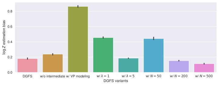
We conduct ablation studies on a series of design choices of DGFS. In Figure 10, we compare the performance of DGFS and a few its variants on the VAE task. In the VAE task, the unnormalized target density $\log\mu(\cdot)$ is defined by the log latent prior $\log p(\cdot)$ plus the log decoder likelihood $\log p(\mathbf{x}_{\text{obs}}|\cdot)$, which equals the latent posterior $\log p(\cdot|\mathbf{x}_{\text{obs}})$ plus a constant value. The VAE is trained on the MNIST dataset, and $\mathbf{x}_{\text{obs}}$ is a fixed image data. We first remove the usage of the intermediate signals (i.e., the parameterization of flow function in Equation 16), which leads to slightly worse performance. We then try to train DGFS with VP modeling in Appendix B.2. For this VP modeling, we also take the form of Equation 16 for getting intermediate signals. This gives a bias of $0.86$. Notice that this is still better than both PIS and DDS, demonstrating the validity of the proposed DGFS training method. We also ablate the weighting coefficient $\lambda$ and number of diffusion steps $N$. We can see their changes lead to small variations but the overall convergence remains good.

Regarding the running time of the proposed algorithm, DGFS has the same inference procedure as PIS, and thus having the same inference speed as PIS. The training overhead of DGFS is slightly ($20\%$) higher than PIS due to the introduction of the additional flow function network. In the Funnel task, the training time of DGFS and PIS for one batch are $0.54$s and $0.65$s respectively.

We then show some missing results from the main text. We put the visualization of the joint of the second and third dimension in Manywell task in Figure 8. We can see that PIS misses one important mode and DDS could not handle the mode separation well enough.

We tried to use a MNIST-pretrained normalizing flow as the target density. However, we find a well-trained normalizing flow almost always assign $-\infty$ to the log likelihood for out-of-distribution samples, which makes it impossible for any sampler to success. This actually makes sense as the normalizing flow is only trained on a finite size image dataset and never gets out-of-domain inputs.

C.6 Remove gradient information from parametrization

Table 2: Experimental results on benchmarking target densities, where the diffusion-based samplers are not allowed to directly access gradient information of the target log density in the drift network design. Note the PIS-NN and DDS-NN here still require to know the gradient information due to their KL formulation, while the DGFS-NN here is a real black-box algorithm and only need to know zeroth order information from the target.

	MoG	Funnel	Manywell	VAE	Cox
PIS-NN (w/ gradient)	$1.943$$\pm 0.259$	$0.374$$\pm 0.024$	$2.712$$\pm 0.017$	$0.368$$\pm 0.064$	$85.36$$\pm 3.342$
DDS-NN (w/ gradient)	$2.183$$\pm 0.018$	$0.351$$\pm 0.022$	$4.056$$\pm 1.195$	$1.740$$\pm 1.158$	N/A
DGFS-NN	${0.023}$$\pm 0.001$	${0.354}$$\pm 0.072$	${2.659}$$\pm 0.057$	${0.496}$$\pm 0.196$	$109.0$$\pm 4.344$

In the network design, PIS explicitly use the score function—gradient of the log unnormalized density function—as one term in the drift network parametrization. Our work and DDS follow its modeling. In this section, we show performance where the score function are removed from the architecture of all three diffusion-base samplers in Table 2. We attach “-NN” postfix to their names to distinguish between their original algorithms. Notice PIS-NN and DDS-NN still require the knowledge of the score function implicitly based on their KL formulation. On the other hand, DGFS-NN is a real black-box method, i.e., only requires zeroth order information of the unnormalized density function. Despite using less information, DGFS-NN is still very competitive in most of the tasks.

C.7 Off-policy exploration ability of DGFS

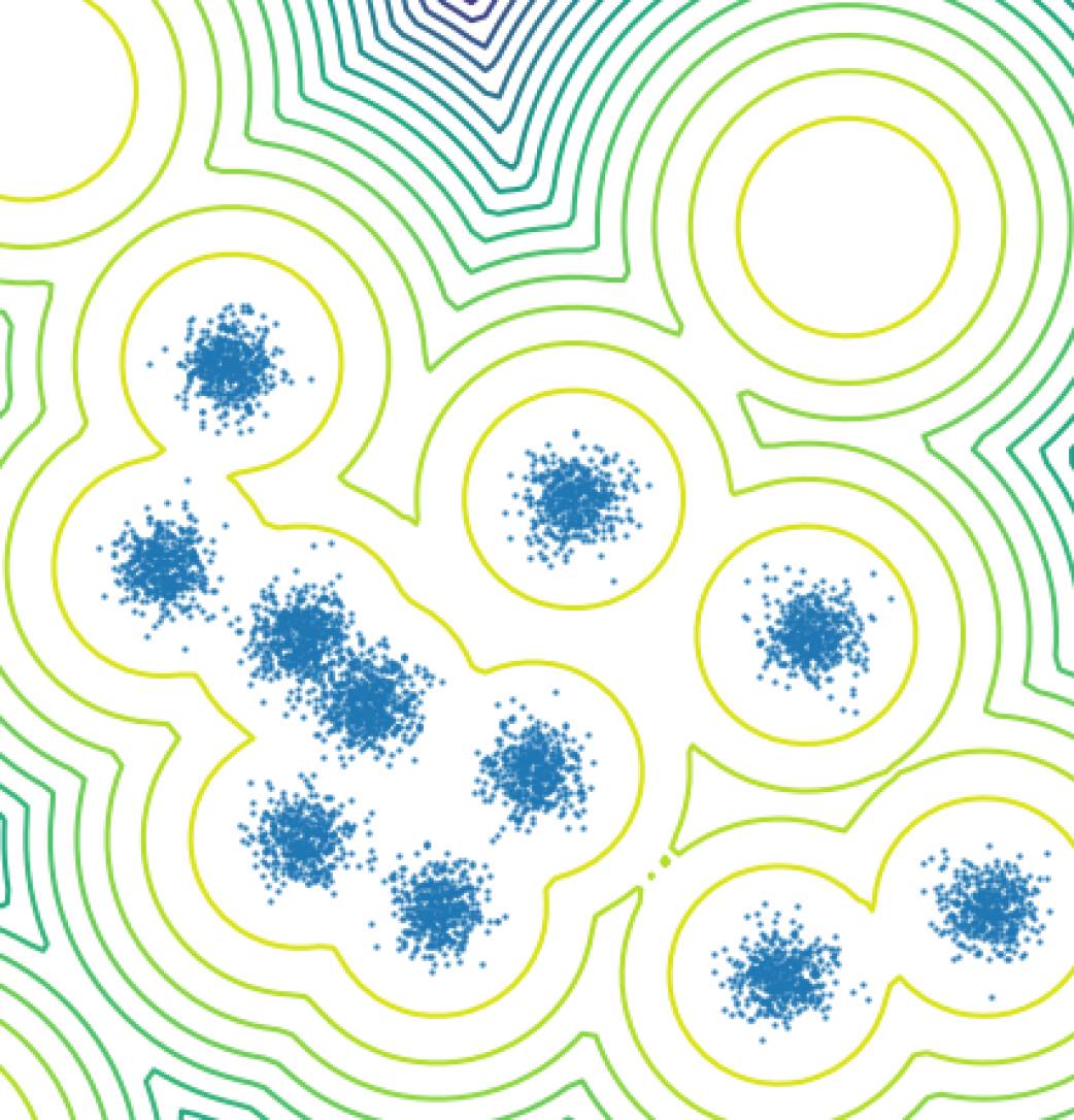
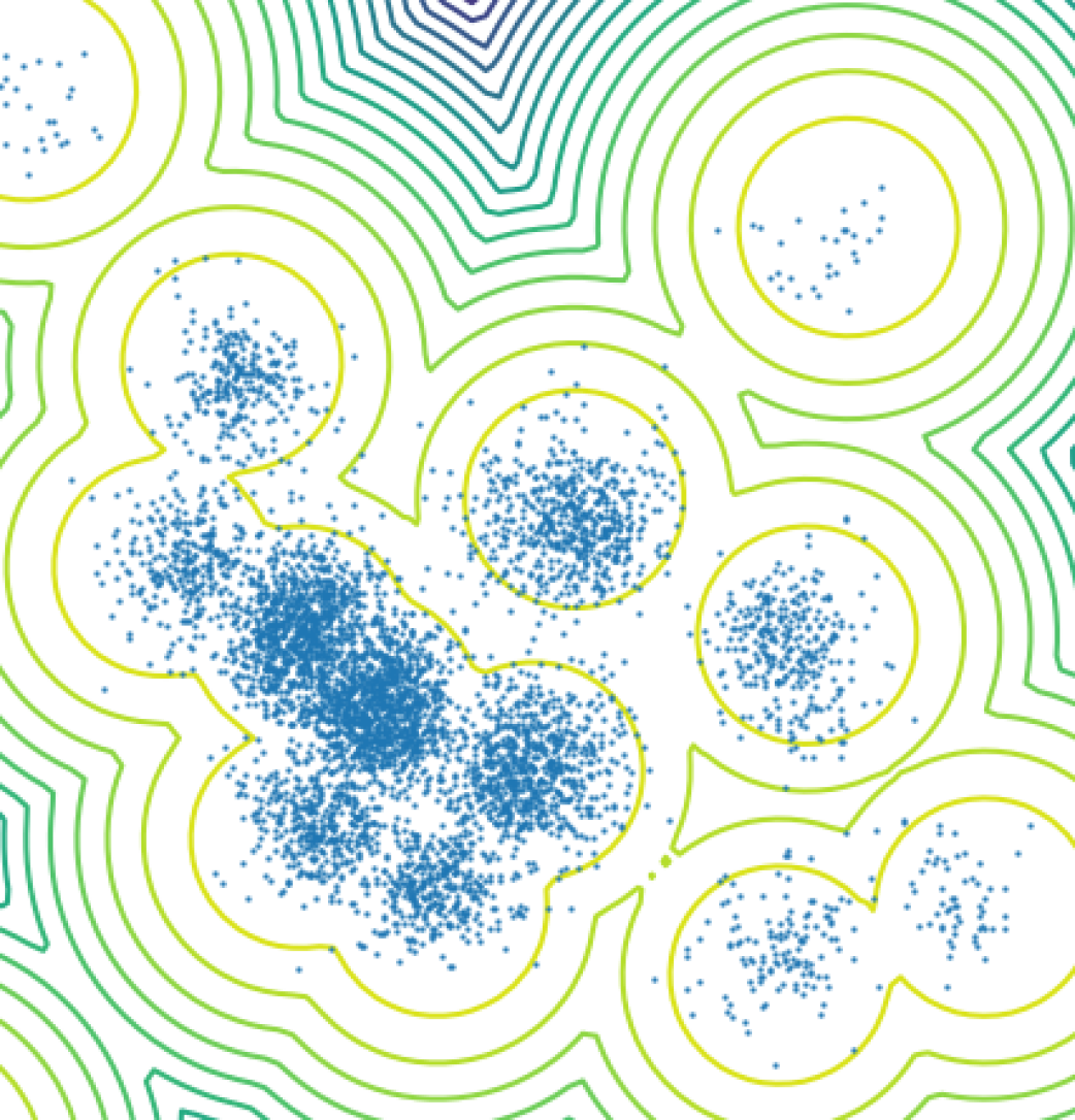
The usage of the KL divergence in previous works restricts the training to be on-policy, as the training trajectory has to come from the model itself. Using off-policy samples is possible only with importance sampling, which typically results in high variance. This limits the exploration ability of these methods. On the other hand, it is first shown in Malkin et al. (2023) that GFlowNets can potentially benefit from the use of off-policy exploration. To be more specific, as has been shown by a similar analysis in prior works Malkin et al. (2023); Lahlou et al. (2023), the objectives in Equation 9 or Equation 14 do not require the training samples to follow any particular distribution (only to have full support), which means our method supports off-policy training without importance sampling. Therefore, it is possible to employ off-policy exploration by using a larger variance coefficient in the forward process during the rollout stage. In theory, this could help DGFS to better capture diversity in complex multimodal target distributions.

In an algorithmic perspective, we could use a slightly larger variance coefficient $\tilde{\sigma}>\sigma$ in the rollout stage of Algorithm 1 to ensure that information of more modes fall into the training data, which would drive the training of DGFS to put effort on these distant modes. To demonstrate this property, we carefully create a more difficult Mixture of Gaussian task and name it as MoG+. We intentionally put a few very distant modes in this MoG+ task, as shown by the contours in Figure 9. We set the exploration variance coefficient $\tilde{\sigma}=2$ contrary to $\sigma=1$, which achieves better mode coverage and lower normalizing factor estimation bias with the same neural network capacity.

We conduct an initial experiment to investigate this possibility in DGFS. We test a strategy that linearly anneals the $\tilde{\sigma}$ from $1.1$ to $1$ during the first $1000$ steps of training, and denote it as DGFS+ in Table 3. Our experiment results show that this simple strategy can improve the performance under some scenarios, and can be treated as a potential hyperparameter to extend the application scope of DGFS.

Table 3: Experimental results on benchmarking target densities. DGFS+ denotes DGFS with additional off-policy exploration trick in the initial stage of training.

	MoG	Funnel	Manywell	VAE	Cox
DGFS	${0.019}$$\pm 0.008$	${0.274}$$\pm 0.014$	${0.904}$$\pm 0.067$	${0.180}$$\pm 0.083$	${8.974}$$\pm 1.169$
DGFS+	$0.012$$\pm 0.002$	$0.322$$\pm 0.029$	$0.932$$\pm 0.123$	$0.162$$\pm 0.015$	$10.23$$\pm 1.237$

C.8 Other ablation study

Table 4: Experimental results on benchmarking target densities for methods in Lahlou et al. (2023), with or without off-policy exploration technique. We also present performance of TB and its off-policy variant; see details in Section C.8.

	MoG	Funnel	Manywell	VAE	Cox
Lahlou et al. (2023)	${1.891}$$\pm 0.042$	${0.398}$$\pm 0.061$	${3.669}$$\pm 0.653$	${4.563}$$\pm 1.029$	${2728.}$$\pm 51.54$
Lahlou et al. (2023)+	$0.024$$\pm 0.189$	$0.373$$\pm 0.020$	$6.257$$\pm 2.449$	$2.529$$\pm 0.737$	$2722.$$\pm 31.64$
TB	${0.018}$$\pm 0.002$	${0.309}$$\pm 0.023$	${1.218}$$\pm 0.194$	${1.097}$$\pm 0.239$	${138.6}$$\pm 7.850$
TB+	${0.009}$$\pm 0.003$	${0.373}$$\pm 0.031$	${1.210}$$\pm 0.192$	${0.842}$$\pm 0.248$	${240.4}$$\pm 0.998$

We run the method in Lahlou et al. (2023) in this section. As shown in Table 4, this previous method and its off-policy variant are far from comparable to the baselines in Table 1. We also run the trajectory balance method with gradient information (denoted as TB) and its variant with off-policy exploration (denoted as TB+) and present in the same table. These two methods achieve relatively better performance, but still worse than that of DGFS.

References

- Albergo et al. (2019) Michael S Albergo, Gurtej Kanwar, and Phiala E. Shanahan. Flow-based generative models for markov chain monte carlo in lattice field theory. ArXiv, abs/1904.12072, 2019. URL https://api.semanticscholar.org/CorpusID:139104868.
- Andrieu et al. (2004) Christophe Andrieu, Nando de Freitas, A. Doucet, and Michael I. Jordan. An introduction to mcmc for machine learning. Machine Learning, 50:5–43, 2004. URL https://api.semanticscholar.org/CorpusID:38363.
- Arbel et al. (2021) Michal Arbel, Alexander G. de G. Matthews, and A. Doucet. Annealed flow transport monte carlo. ArXiv, abs/2102.07501, 2021. URL https://api.semanticscholar.org/CorpusID:231925352.
- Atanackovic et al. (2023) Lazar Atanackovic, Alexander Tong, Jason S. Hartford, Leo J. Lee, Bo Wang, and Yoshua Bengio. Dyngfn: Bayesian dynamic causal discovery using generative flow networks. ArXiv, abs/2302.04178, 2023. URL https://api.semanticscholar.org/CorpusID:256662181.
- Bengio et al. (2021) Emmanuel Bengio, Moksh Jain, Maksym Korablyov, Doina Precup, and Yoshua Bengio. Flow network based generative models for non-iterative diverse candidate generation. Neural Information Processing Systems (NeurIPS), 2021.
- Bengio et al. (2023) Yoshua Bengio, Salem Lahlou, Tristan Deleu, Edward J Hu, Mo Tiwari, and Emmanuel Bengio. GFlowNet foundations. Journal of Machine Learning Research, (24):1–76, 2023.
- Berner et al. (2022) Julius Berner, Lorenz Richter, and Karen Ullrich. An optimal control perspective on diffusion-based generative modeling. ArXiv, abs/2211.01364, 2022. URL https://api.semanticscholar.org/CorpusID:253255370.
- Blei et al. (2016) David M. Blei, Alp Kucukelbir, and Jon D. McAuliffe. Variational inference: A review for statisticians. ArXiv, abs/1601.00670, 2016. URL https://api.semanticscholar.org/CorpusID:3554631.
- Bortoli (2022) Valentin De Bortoli. Convergence of denoising diffusion models under the manifold hypothesis. ArXiv, abs/2208.05314, 2022. URL https://api.semanticscholar.org/CorpusID:251468296.
- Brooks et al. (2011) Steve P. Brooks, Andrew Gelman, Galin L. Jones, and Xiao-Li Meng. Handbook of markov chain monte carlo. 2011. URL https://api.semanticscholar.org/CorpusID:60438653.
- Burda et al. (2016) Yuri Burda, Roger Baker Grosse, and Ruslan Salakhutdinov. Importance weighted autoencoders. International Conference on Learning Representations (ICLR), 2016.
- Caselle et al. (2022) Michele Caselle, Elia Cellini, Alessandro Nada, and Marco Panero. Stochastic normalizing flows as non-equilibrium transformations. Journal of High Energy Physics, 2022, 2022. URL https://api.semanticscholar.org/CorpusID:246240579.
- Chen et al. (2022) Sitan Chen, Sinho Chewi, Jungshian Li, Yuanzhi Li, Adil Salim, and Anru R. Zhang. Sampling is as easy as learning the score: theory for diffusion models with minimal data assumptions. ArXiv, abs/2209.11215, 2022. URL https://api.semanticscholar.org/CorpusID:252438904.
- Chen et al. (2018) Tian Qi Chen, Yulia Rubanova, Jesse Bettencourt, and David Kristjanson Duvenaud. Neural ordinary differential equations. In Neural Information Processing Systems, 2018. URL https://api.semanticscholar.org/CorpusID:49310446.
- Chen et al. (2014) Tianqi Chen, Emily B. Fox, and Carlos Guestrin. Stochastic gradient hamiltonian monte carlo. In International Conference on Machine Learning, 2014. URL https://api.semanticscholar.org/CorpusID:3228832.
- Chen et al. (2020) Yanzhi Chen, Dinghuai Zhang, Michael U Gutmann, Aaron C. Courville, and Zhanxing Zhu. Neural approximate sufficient statistics for implicit models. ArXiv, abs/2010.10079, 2020. URL https://api.semanticscholar.org/CorpusID:224804162.
- de G. Matthews et al. (2022) Alexander G. de G. Matthews, Michal Arbel, Danilo Jimenez Rezende, and A. Doucet. Continual repeated annealed flow transport monte carlo. ArXiv, abs/2201.13117, 2022. URL https://api.semanticscholar.org/CorpusID:246430223.
- Deleu et al. (2022) Tristan Deleu, António Góis, Chris Emezue, Mansi Rankawat, Simon Lacoste-Julien, Stefan Bauer, and Yoshua Bengio. Bayesian structure learning with generative flow networks. Uncertainty in Artificial Intelligence (UAI), 2022.
- Deleu et al. (2023) Tristan Deleu, Mizu Nishikawa-Toomey, Jithendaraa Subramanian, Nikolay Malkin, Laurent Charlin, and Yoshua Bengio. Joint Bayesian inference of graphical structure and parameters with a single generative flow network. arXiv preprint arXiv:2305.19366, 2023.
- Desjardins et al. (2010) Guillaume Desjardins, Aaron C. Courville, Yoshua Bengio, Pascal Vincent, and Olivier Delalleau. Tempered markov chain monte carlo for training of restricted boltzmann machines. In International Conference on Artificial Intelligence and Statistics, 2010. URL https://api.semanticscholar.org/CorpusID:16382829.
- Dinh et al. (2014) Laurent Dinh, David Krueger, and Yoshua Bengio. Nice: Non-linear independent components estimation. CoRR, abs/1410.8516, 2014. URL https://api.semanticscholar.org/CorpusID:13995862.
- Doucet et al. (2001) A. Doucet, Nando de Freitas, and Neil J. Gordon. Sequential monte carlo methods in practice. In Statistics for Engineering and Information Science, 2001. URL https://api.semanticscholar.org/CorpusID:30176573.
- Doucet et al. (2022) A. Doucet, Will Grathwohl, Alexander G. de G. Matthews, and Heiko Strathmann. Score-based diffusion meets annealed importance sampling. ArXiv, abs/2208.07698, 2022. URL https://api.semanticscholar.org/CorpusID:251594572.
- Du et al. (2022) Weitao Du, Tao Yang, Heidi Zhang, and Yuanqi Du. A flexible diffusion model. ArXiv, abs/2206.10365, 2022. URL https://api.semanticscholar.org/CorpusID:249889644.
- Duane et al. (1987) Simon Duane, Anthony D. Kennedy, Brian Pendleton, and Duncan Roweth. Hybrid monte carlo. 1987. URL https://api.semanticscholar.org/CorpusID:121101759.
- Frenkel & Smit (1996) Daan Frenkel and Berend Smit. Understanding molecular simulation: from algorithms to applications. 1996. URL https://api.semanticscholar.org/CorpusID:62612337.
- Gabri’e et al. (2021) Marylou Gabri’e, Grant M. Rotskoff, and Eric Vanden-Eijnden. Adaptive monte carlo augmented with normalizing flows. Proceedings of the National Academy of Sciences of the United States of America, 119, 2021. URL https://api.semanticscholar.org/CorpusID:235195952.
- Gao et al. (2020) Christina Gao, Joshua Isaacson, and Claudius Krause. i-flow: High-dimensional integration and sampling with normalizing flows. Machine Learning: Science and Technology, 1, 2020. URL https://api.semanticscholar.org/CorpusID:210701113.
- Geffner & Domke (2022) Tomas Geffner and Justin Domke. Langevin diffusion variational inference. In International Conference on Artificial Intelligence and Statistics, 2022. URL https://api.semanticscholar.org/CorpusID:251594511.
- Hernández-García et al. (2023) Alex Hernández-García, Nikita Saxena, Moksh Jain, Cheng-Hao Liu, and Yoshua Bengio. Multi-fidelity active learning with gflownets. ArXiv, abs/2306.11715, 2023. URL https://api.semanticscholar.org/CorpusID:259202477.
- Hernández-Lobato & Adams (2015) José Miguel Hernández-Lobato and Ryan P. Adams. Probabilistic backpropagation for scalable learning of bayesian neural networks. In International Conference on Machine Learning, 2015. URL https://api.semanticscholar.org/CorpusID:8645175.
- Ho et al. (2020a) Jonathan Ho, Ajay Jain, and P. Abbeel. Denoising diffusion probabilistic models. ArXiv, abs/2006.11239, 2020a. URL https://api.semanticscholar.org/CorpusID:219955663.
- Ho et al. (2020b) Jonathan Ho, Ajay Jain, and Pieter Abbeel. Denoising diffusion probabilistic models. Neural Information Processing Systems (NeurIPS), 2020b.
- Hoffman & Gelman (2011) Matthew D. Hoffman and Andrew Gelman. The no-u-turn sampler: adaptively setting path lengths in hamiltonian monte carlo. J. Mach. Learn. Res., 15:1593–1623, 2011. URL https://api.semanticscholar.org/CorpusID:12948548.
- Holdijk et al. (2022) Lars Holdijk, Yuanqi Du, Ferry Hooft, Priyank Jaini, Bernd Ensing, and Max Welling. Stochastic optimal control for collective variable free sampling of molecular transition paths. 2022. URL https://api.semanticscholar.org/CorpusID:259951301.
- Hollingsworth & Dror (2018) Scott A. Hollingsworth and Ron O. Dror. Molecular dynamics simulation for all. Neuron, 99:1129–1143, 2018. URL https://api.semanticscholar.org/CorpusID:52311344.
- Hu et al. (2023) Edward J Hu, Nikolay Malkin, Moksh Jain, Katie Everett, Alexandros Graikos, and Yoshua Bengio. GFlowNet-EM for learning compositional latent variable models. International Conference on Machine Learning (ICML), 2023.
- Jain et al. (2022) Moksh Jain, Emmanuel Bengio, Alex Hernandez-Garcia, Jarrid Rector-Brooks, Bonaventure F.P. Dossou, Chanakya Ekbote, Jie Fu, Tianyu Zhang, Micheal Kilgour, Dinghuai Zhang, Lena Simine, Payel Das, and Yoshua Bengio. Biological sequence design with GFlowNets. International Conference on Machine Learning (ICML), 2022.
- Jain et al. (2023a) Moksh Jain, Tristan Deleu, Jason S. Hartford, Cheng-Hao Liu, Alex Hernández-García, and Yoshua Bengio. Gflownets for ai-driven scientific discovery. ArXiv, abs/2302.00615, 2023a. URL https://api.semanticscholar.org/CorpusID:256459319.
- Jain et al. (2023b) Moksh Jain, Sharath Chandra Raparthy, Alex Hernandez-Garcia, Jarrid Rector-Brooks, Yoshua Bengio, Santiago Miret, and Emmanuel Bengio. Multi-objective GFlowNets. International Conference on Machine Learning (ICML), 2023b.
- Kappen (2005) Hilbert J Kappen. Path integrals and symmetry breaking for optimal control theory. Journal of statistical mechanics: theory and experiment, 2005(11):P11011, 2005.
- Kearns & Singh (2000) Michael Kearns and Satinder Singh. Bias-variance error bounds for temporal difference updates. In Annual Conference Computational Learning Theory, 2000. URL https://api.semanticscholar.org/CorpusID:5053575.
- Kingma & Welling (2014) Diederik P. Kingma and Max Welling. Auto-encoding variational Bayes. International Conference on Learning Representations (ICLR), 2014.
- Lahlou et al. (2023) Salem Lahlou, Tristan Deleu, Pablo Lemos, Dinghuai Zhang, Alexandra Volokhova, Alex Hernández-García, Léna Néhale Ezzine, Yoshua Bengio, and Nikolay Malkin. A theory of continuous generative flow networks. International Conference on Machine Learning (ICML), 2023.
- Lee et al. (2022) Holden Lee, Jianfeng Lu, and Yixin Tan. Convergence of score-based generative modeling for general data distributions. ArXiv, abs/2209.12381, 2022. URL https://api.semanticscholar.org/CorpusID:252531877.
- Li et al. (2023a) Wenqian Li, Yinchuan Li, Zhigang Li, Jianye Hao, and Yan Pang. Dag matters! gflownets enhanced explainer for graph neural networks. ArXiv, abs/2303.02448, 2023a. URL https://api.semanticscholar.org/CorpusID:257365860.
- Li et al. (2023b) Yinchuan Li, Shuang Luo, Haozhi Wang, and Jianye Hao. CFlowNets: Continuous control with generative flow networks. International Conference on Learning Representations (ICLR), 2023b.
- Liu et al. (2022) Dianbo Liu, Moksh Jain, Bonaventure F. P. Dossou, Qianli Shen, Salem Lahlou, Anirudh Goyal, Nikolay Malkin, Chris C. Emezue, Dinghuai Zhang, Nadhir Hassen, Xu Ji, Kenji Kawaguchi, and Yoshua Bengio. Gflowout: Dropout with generative flow networks. In International Conference on Machine Learning, 2022. URL https://api.semanticscholar.org/CorpusID:253097963.
- Liu (2001) Jun S. Liu. Monte carlo strategies in scientific computing. 2001. URL https://api.semanticscholar.org/CorpusID:62226424.
- Madan et al. (2022) Kanika Madan, Jarrid Rector-Brooks, Maksym Korablyov, Emmanuel Bengio, Moksh Jain, Andrei Nica, Tom Bosc, Yoshua Bengio, and Nikolay Malkin. Learning GFlowNets from partial episodes for improved convergence and stability. International Conference on Machine Learning (ICML), 2022.
- Malkin et al. (2023) Nikolay Malkin, Salem Lahlou, Tristan Deleu, Xu Ji, Edward Hu, Katie Everett, Dinghuai Zhang, and Yoshua Bengio. GFlowNets and variational inference. International Conference on Learning Representations (ICLR), 2023.
- Midgley et al. (2022) Laurence Illing Midgley, Vincent Stimper, Gregor N. C. Simm, Bernhard Schölkopf, and José Miguel Hernández-Lobato. Flow annealed importance sampling bootstrap. ArXiv, abs/2208.01893, 2022. URL https://api.semanticscholar.org/CorpusID:251280102.
- Minka (2001) Thomas P. Minka. Expectation propagation for approximate Bayesian inference. arXiv preprint arXiv:1301.2294, 2001.
- Møller et al. (1998) Jesper M. Møller, Anne Randi Syversveen, and Rasmus Waagepetersen. Log gaussian cox processes. Scandinavian Journal of Statistics, 25, 1998. URL https://api.semanticscholar.org/CorpusID:120543073.
- Moral & Doucet (2002) Pierre Del Moral and A. Doucet. Sequential monte carlo samplers. Journal of the Royal Statistical Society: Series B (Statistical Methodology), 68, 2002. URL https://api.semanticscholar.org/CorpusID:12074789.
- Müller et al. (2018) Thomas Müller, Brian McWilliams, Fabrice Rousselle, Markus H. Gross, and Jan Novák. Neural importance sampling. ACM Transactions on Graphics (TOG), 38:1 – 19, 2018. URL https://api.semanticscholar.org/CorpusID:51970108.
- Neal (1995) Radford M. Neal. Bayesian learning for neural networks. 1995. URL https://api.semanticscholar.org/CorpusID:251471788.
- Neal (1998) Radford M. Neal. Annealed importance sampling. Statistics and Computing, 11:125–139, 1998. URL https://api.semanticscholar.org/CorpusID:11112994.
- Neal (2003) Radford M. Neal. Slice sampling. The Annals of Statistics, 31(3), Jun 2003. ISSN 0090-5364. doi: 10.1214/aos/1056562461. URL http://dx.doi.org/10.1214/aos/1056562461.
- Nicoli et al. (2020) Kim A. Nicoli, Shinichi Nakajima, Nils Strodthoff, Wojciech Samek, Klaus-Robert Müller, and Pan Kessel. Asymptotically unbiased estimation of physical observables with neural samplers. Physical review. E, 101 2-1:023304, 2020. URL https://api.semanticscholar.org/CorpusID:211096944.
- Nicoli et al. (2021) Kim A. Nicoli, Christopher J. Anders, Lena Funcke, Tobias Hartung, Karl Jansen, Pan Kessel, Shinichi Nakajima, and Paolo Stornati. Estimation of thermodynamic observables in lattice field theories with deep generative models. Physical review letters, 126 3:032001, 2021. URL https://api.semanticscholar.org/CorpusID:220514403.
- Nicoli et al. (2023) Kim A. Nicoli, Christopher J. Anders, Tobias Hartung, Karl Jansen, Pan Kessel, and Shinichi Nakajima. Detecting and mitigating mode-collapse for flow-based sampling of lattice field theories. ArXiv, abs/2302.14082, 2023. URL https://api.semanticscholar.org/CorpusID:257232703.
- Noé et al. (2019) Frank Noé, Jonas Köhler, and Hao Wu. Boltzmann generators: Sampling equilibrium states of many-body systems with deep learning. Science, 365, 2019. URL https://api.semanticscholar.org/CorpusID:54458652.
- Pan et al. (2023a) Ling Pan, Nikolay Malkin, Dinghuai Zhang, and Yoshua Bengio. Better training of GFlowNets with local credit and incomplete trajectories. International Conference on Machine Learning (ICML), 2023a.
- Pan et al. (2023b) Ling Pan, Dinghuai Zhang, Aaron Courville, Longbo Huang, and Yoshua Bengio. Generative augmented flow networks. International Conference on Learning Representations (ICLR), 2023b.
- Pan et al. (2023c) Ling Pan, Dinghuai Zhang, Moksh Jain, Longbo Huang, and Yoshua Bengio. Stochastic generative flow networks. Uncertainty in Artificial Intelligence (UAI), 2023c.
- Rezende & Mohamed (2015) Danilo Jimenez Rezende and Shakir Mohamed. Variational inference with normalizing flows. ArXiv, abs/1505.05770, 2015. URL https://api.semanticscholar.org/CorpusID:12554042.
- Rezende et al. (2014) Danilo Jimenez Rezende, Shakir Mohamed, and Daan Wierstra. Stochastic backpropagation and approximate inference in deep generative models. International Conference on Machine Learning (ICML), 2014.
- Richter et al. (2023) Lorenz Richter, Julius Berner, and Guan-Horng Liu. Improved sampling via learned diffusions. ArXiv, abs/2307.01198, 2023. URL https://api.semanticscholar.org/CorpusID:259316542.
- Roeder et al. (2017) Geoffrey Roeder, Yuhuai Wu, and David Kristjanson Duvenaud. Sticking the landing: Simple, lower-variance gradient estimators for variational inference. In NIPS, 2017. URL https://api.semanticscholar.org/CorpusID:30321501.
- Shen et al. (2023) Max W. Shen, Emmanuel Bengio, Ehsan Hajiramezanali, Andreas Loukas, Kyunghyun Cho, and Tommaso Biancalani. Towards understanding and improving gflownet training. ArXiv, abs/2305.07170, 2023. URL https://api.semanticscholar.org/CorpusID:258676487.
- Sohl-Dickstein et al. (2015) Jascha Narain Sohl-Dickstein, Eric A. Weiss, Niru Maheswaranathan, and Surya Ganguli. Deep unsupervised learning using nonequilibrium thermodynamics. ArXiv, abs/1503.03585, 2015. URL https://api.semanticscholar.org/CorpusID:14888175.
- Song et al. (2020) Yang Song, Jascha Narain Sohl-Dickstein, Diederik P. Kingma, Abhishek Kumar, Stefano Ermon, and Ben Poole. Score-based generative modeling through stochastic differential equations. ArXiv, abs/2011.13456, 2020. URL https://api.semanticscholar.org/CorpusID:227209335.
- Sutton & Barto (2018) Richard S Sutton and Andrew G Barto. Reinforcement learning: An introduction. MIT press, 2018.
- Tieleman & Hinton (2009) Tijmen Tieleman and Geoffrey E. Hinton. Using fast weights to improve persistent contrastive divergence. In International Conference on Machine Learning, 2009. URL https://api.semanticscholar.org/CorpusID:415956.
- Tzen & Raginsky (2019) Belinda Tzen and Maxim Raginsky. Theoretical guarantees for sampling and inference in generative models with latent diffusions. In Annual Conference Computational Learning Theory, 2019. URL https://api.semanticscholar.org/CorpusID:71148500.
- Vaitl et al. (2022a) Lorenz Vaitl, Kim A. Nicoli, Shinichi Nakajima, and Pan Kessel. Gradients should stay on path: better estimators of the reverse- and forward kl divergence for normalizing flows. Machine Learning: Science and Technology, 3, 2022a. URL https://api.semanticscholar.org/CorpusID:250626584.
- Vaitl et al. (2022b) Lorenz Vaitl, Kim A. Nicoli, Shinichi Nakajima, and Pan Kessel. Path-gradient estimators for continuous normalizing flows. ArXiv, abs/2206.09016, 2022b. URL https://api.semanticscholar.org/CorpusID:249890240.
- Vargas & Nusken (2023) Francisco Vargas and Nikolas Nusken. Transport, variational inference and diffusions: with applications to annealed flows and schrödinger bridges. ArXiv, abs/2307.01050, 2023. URL https://api.semanticscholar.org/CorpusID:259317037.
- Vargas et al. (2021) Francisco Vargas, Andrius Ovsianas, David Fernandes, Mark A. Girolami, Neil D. Lawrence, and Nikolas Nusken. Bayesian learning via neural schrödinger–föllmer flows. Statistics and Computing, 33, 2021. URL https://api.semanticscholar.org/CorpusID:244477794.
- Vargas et al. (2023a) Francisco Vargas, Will Grathwohl, and A. Doucet. Denoising diffusion samplers. ArXiv, abs/2302.13834, 2023a. URL https://api.semanticscholar.org/CorpusID:257220165.
- Vargas et al. (2023b) Francisco Vargas, Teodora Reu, and Anna Kerekes. Expressiveness remarks for denoising diffusion models and samplers. ArXiv, abs/2305.09605, 2023b. URL https://api.semanticscholar.org/CorpusID:258715268.
- Vincent (2011) Pascal Vincent. A connection between score matching and denoising autoencoders. Neural Computation, 23:1661–1674, 2011. URL https://api.semanticscholar.org/CorpusID:5560643.
- Welling & Teh (2011) Max Welling and Yee Whye Teh. Bayesian learning via stochastic gradient langevin dynamics. In International Conference on Machine Learning, 2011. URL https://api.semanticscholar.org/CorpusID:2178983.
- Wirnsberger et al. (2020) Peter Wirnsberger, Andrew J. Ballard, George Papamakarios, Stuart Abercrombie, Sébastien Racanière, Alexander Pritzel, Danilo Jimenez Rezende, and Charles Blundell. Targeted free energy estimation via learned mappings. The Journal of chemical physics, 153 14:144112, 2020. URL https://api.semanticscholar.org/CorpusID:211082968.
- Wu et al. (2018) Dian Wu, Lei Wang, and Pan Zhang. Solving statistical mechanics using variational autoregressive networks. Physical review letters, 122 8:080602, 2018. URL https://api.semanticscholar.org/CorpusID:52879890.
- Wu et al. (2020) Hao Wu, Jonas Köhler, and Frank No’e. Stochastic normalizing flows. ArXiv, abs/2002.06707, 2020. URL https://api.semanticscholar.org/CorpusID:211133098.
- Xu et al. (2022) Winnie Xu, Ricky T. Q. Chen, Xuechen Li, and David Duvenaud. Infinitely deep bayesian neural networks with stochastic differential equations. In International Conference on Artificial Intelligence and Statistics, pp. 721–738. PMLR, 2022.
- Zhang et al. (2023a) David W. Zhang, Corrado Rainone, Markus F. Peschl, and Roberto Bondesan. Robust scheduling with gflownets. ArXiv, abs/2302.05446, 2023a. URL https://api.semanticscholar.org/CorpusID:256827133.
- Zhang et al. (2021) Dinghuai Zhang, Jie Fu, Yoshua Bengio, and Aaron C. Courville. Unifying likelihood-free inference with black-box optimization and beyond. In International Conference on Learning Representations, 2021. URL https://api.semanticscholar.org/CorpusID:246680129.
- Zhang et al. (2022a) Dinghuai Zhang, Ricky T. Q. Chen, Nikolay Malkin, and Yoshua Bengio. Unifying generative models with GFlowNets and beyond. arXiv preprint arXiv:2209.02606v2, 2022a.
- Zhang et al. (2022b) Dinghuai Zhang, Nikolay Malkin, Zhen Liu, Alexandra Volokhova, Aaron Courville, and Yoshua Bengio. Generative flow networks for discrete probabilistic modeling. International Conference on Machine Learning (ICML), 2022b.
- Zhang et al. (2023b) Dinghuai Zhang, Hanjun Dai, Nikolay Malkin, Aaron C. Courville, Yoshua Bengio, and Ling Pan. Let the flows tell: Solving graph combinatorial optimization problems with gflownets. ArXiv, abs/2305.17010, 2023b. URL https://api.semanticscholar.org/CorpusID:258947700.
- Zhang et al. (2023c) Dinghuai Zhang, L. Pan, Ricky T. Q. Chen, Aaron C. Courville, and Yoshua Bengio. Distributional gflownets with quantile flows. arXiv preprint arXiv:2302.05793, 2023c.
- Zhang & Chen (2022) Qinsheng Zhang and Yongxin Chen. Path integral sampler: a stochastic control approach for sampling. International Conference on Learning Representations (ICLR), 2022.
- Zimmermann et al. (2022) Heiko Zimmermann, Fredrik Lindsten, J.-W. van de Meent, and Christian Andersson Naesseth. A variational perspective on generative flow networks. ArXiv, abs/2210.07992, 2022. URL https://api.semanticscholar.org/CorpusID:252907672.