Generative Modeling of Regular and Irregular Time Series Data via Koopman VAEs

Abstract

Generating realistic time series data is important for many engineering and scientific applications. Existing work tackles this problem using generative adversarial networks (GANs). However, GANs are often unstable during training, and they can suffer from mode collpase. While variational autoencoders (VAEs) are known to be more robust to the these issues, they are (surprisingly) less often considered for time series generation. In this work, we introduce Koopman VAE (KVAE), a new generative framework that is based on a novel design for the model prior, and that can be optimized for either regular and irregular training data. Inspired by Koopman theory, we represent the latent conditional prior dynamics using a linear map. Our approach enhances generative modeling with two desired features: (i) incorporating domain knowledge can be achieved by leverageing spectral tools that prescribe constraints on the eigenvalues of the linear map; and (ii) studying the qualitative behavior and stablity of the system can be performed using tools from dynamical systems theory. Our results show that KVAE outperforms state-of-the-art GAN and VAE methods across several challenging synthetic and real-world time series generation benchmarks. Whether trained on regular or irregular data, KVAE generates time series that improve both discriminative and predictive metrics. We also present visual evidence suggesting that KVAE learns probability density functions that better approximate empirical ground truth distributions.

1 Introduction

Generative modeling is an important problem in modern machine learning (Kingma & Welling, 2014; Goodfellow et al., 2014; Sohl-Dickstein et al., 2015), with a recent surge in interest due to results in natural language processing (Brown et al., 2020) and computer vision (Rombach et al., 2022; Ramesh et al., 2022). While image and text data have benefitted from the recent development of generative models, time series (TS) data has received relatively little attention. This is in spite of the importance of generating TS data in various scientific and engineering domains, including seismology, climate studies, and energy analysis. Since these fields can face challenges in collecting sufficient data, e.g., due to high computational costs or limited sensor availability, high-quality generative models could be invaluable. However, generating TS data (in particular for scientific and engineering problems) presents its own unique set of challenges. First, any generated TS must preserve relevant statistical distributions to fit into downstream forecasting, uncertainty quantification, and domain classification tasks. Second, advanced objectives such as supporting irregular sampling and integrating domain knowledge require models and tools that respect the underlying dynamics (Che et al., 2018; Kidger et al., 2020; Jeon et al., 2022; Coletta et al., 2023).

Several existing state-of-the-art (SOTA) generative TS models are based on generative adversarial networks (GANs). For example, TimeGAN (Yoon et al., 2019) learns an embedding space where adversarial and supervised losses are optimized to mimic the data dynamics. Unfortunately, GANs are unstable during training, and they are prone to mode collapse, where the learned distribution is not sufficiently expressive (Goodfellow, 2016; Lucic et al., 2018; Saxena & Cao, 2021). In addition, train sets with missing values or, more generally, non-equispaced (irregularly-sampled) measurements, may be not straightforward to support in GAN architectures. For instance, Jeon et al. (2022) combine multiple different technologies to handle irregularly-sampled data, resulting in a complex system with many hyper-parameters. These challenges suggest that other generative paradigms should be also considered for generating TS information.

Surprisingly, variational autoencoders (VAEs) are not considered as strong baselines in generative TS benchmarks (Ang et al., 2023), although they suffer less from unstable training and mode collapse. In these models, an approximate posterior is learned via a neural network to match a certain prior distribution that is assumed to span the data statistics. Recent approaches, including TimeVAE (Desai et al., 2021) and CR-VAE (Li et al., 2023), do employ a variational viewpoint. However, their prior modeling is based on non-sequential standard Gaussian distributions. Therefore, the learned posterior may struggle to represent properly the latent dynamics (Girin et al., 2021). This issue is further excacerbated if one aims to design advanced sequential objectives. For instance, it is unclear how to incorporate domain knowledge about dynamical systems (e.g., stable dynamics, or slow or fast converging or diverging dynamics) with unstructured Gaussian prior distributions. One promising direction to modeling latent dynamics is via linear approaches, and this has recently been shown to improve performance and analysis (Zeng et al., 2023; Orvieto et al., 2023). More generally, this line of work aligns well with theoretical and numerical tools from the Koopman literature (Koopman, 1931; Rowley et al., 2009; Takeishi et al., 2017). Koopman theory offers an alternative representation for autonomous dynamical systems via linear, albeit infinite-dimensional, operators. Harnessing this insight in practice allows one to design autoencoder networks, yielding finite-dimensional approximate Koopman operators that model the latent dynamics.

In this work, we propose Koopman VAE (KVAE), a novel model that leverages the paradigm of linear latent Koopman dynamics within a VAE setup. KVAE uses a model prior that assumes that the sequential latent information is governed by a linear dynamical system. Namely, the conditional prior distribution of the next latent variable, given the current variable, can be represented using a linear map. Under this assumption, we train an approximate posterior distribution that learns a nonlinear coordinate transformation of the inputs to a linear latent representation. Our approach offers two benefits: (i) it models the underlying dynamics, respecting the sequential nature of the input data; and (ii) it seamlessly allows one to incorporate domain knowledge and study the qualitative behavior of the system by using spectral tools from dynamical systems theory. Moreover, to support irregularly-sampled TS information during training, we integrate into KVAE a time-continuous module based on neural controlled differential equations (NCDE) (Kidger et al., 2020). The advantages of KVAE are paramount as they facilitate the capturing of statistical and physical features of sequential information, and, in addition, imposing physics-constraints and analyzing the dynamics is straightforward.

Contributions.

The main contributions of our work can be summarized as follows:

• We propose a new variational generative TS framework for regular and irregularly-sampled data that is based on a novel prior distribution, assuming an implicit linear latent Koopman representation. Our design and modeling yield a flexible, easy-to-code, and powerful generative TS model.

• We show that our approach facilitates high-level capabilities such as physics-constrained TS generation, by penalizing the eigenvalues of the approximated Koopman operator. We also perform stablity analysis by inspecting the spectrum and its spread.

• We show improved SOTA results in regular and irregular settings on several synthetic and real-world datasets, often surpassing strong baselines such as TimeGAN and GT-GAN by large margins. For instance, on the regular and irregular discriminative task we report a total mean relative improvement of 58% and 49% with respect to the second best approach, respectively.

2 Related Work

Our work is related to generative models for TS as well as Koopman-based methods. Both areas enjoy increased interest in recent years, and thus we focus our discussion on the most related work.

Generative Models for Time Series. Recurrent neural networks (RNNs) and their step-wise predictions have been used to generate sequences in Teacher forcing (Graves, 2013) and Professor forcing (Goyal et al., 2016) approaches. Autoregressive methods such as WaveNet (van den Oord et al., 2016) represent the predictive distribution of each audio sample by probabilistic conditioning on all previous samples, whereas TimeGCI (Jarrett et al., 2021) also incorporates GANs and optimizes a transition policy where the reinforcement signal is provided by a global energy framework trained with contrastive estimation. Flow-based models for generating TS information use normalizing flows for an explicit likelihood distribution (Alaa et al., 2020). Long-range sequences were recentlly treated via state-space models (Zhou et al., 2023).

GANs and VAEs. GAN-based architectures have been shown to be effective for generating TS data. C-RNN-GAN (Mogren, 2016) directly applied GANs to sequential data, using LSTM networks for the generator and the discriminator. Recurrent Conditional GAN (Esteban et al., 2017) extends the latter work by dropping the dependence on the previous output while conditioning on additional inputs. TimeGAN (Yoon et al., 2019) is still one of the SOTA methods, and it jointly optimizes unsupervised and supervised loss terms to preserve the temporal dynamics of the training data during the generation process. COT-GAN (Xu et al., 2020) exploits optimal transport and temporal causal constraints to devise a new adversarial loss. Recently, GT-GAN (Jeon et al., 2022) was proposed as one of the few approaches that support irregular sampling, and it employs autoencoders, GANs, and Neural ODEs (Chen et al., 2018). While GAN techniques are more common in generative TS, there are also a few VAE-based approaches. TimeVAE (Desai et al., 2021) models the whole sequence by a global random variable with a normal Gaussian distribution for a prior, and it introduces trend and seasonality building blocks into the decoder. CR-VAE (Li et al., 2023) learns a Granger causal graph by predicting future data from past observations and using a multi-head decoder acting separately on latent variable coordinates.

Koopman-based Approaches. Koopman techniques have gained increasing interest over the past two decades, with applications ranging across analysis (Rowley et al., 2009; Schmid, 2010; Takeishi et al., 2017; Lusch et al., 2018; Azencot et al., 2019), optimization (Dogra & Redman, 2020; Redman et al., 2022), forecasting (Erichson et al., 2019; Azencot et al., 2020; Wang et al., 2023; Tayal et al., 2023), and disentanglement (Berman et al., 2023), among many others (Budišić et al., 2012; Brunton et al., 2021). Most related to our work are Koopman-based probabilistic models, which have received less attention in the literature. Deep variational Koopman models were introduced in Morton et al. (2019), allowing one to sample from distributions over latent observables for prediction tasks. In Srinivasan & Takeishi (2020), the authors propose a Markov Chain Monte Carlo approach to sample over transfer operators. A mean-field variational inference technique with guaranteed stability was suggested in Pan & Duraisamy (2020) for the analysis and prediction of nonlinear dynamics. Finally, Han et al. (2022) designed a stochastic Koopman neural network for control that models the latent observables via a Gaussian distribution. To the best of our knowledge, our work is the first to combine VAEs and Koopman-based methods for generating regular and irregular TS information.

3 Background

We denote by $x_{1:T}$ a TS input $x_{1:T}=x_{1},\dots,x_{T}$, where $x_{t}\in\mathbb{R}^{d}$ for all $t$. In what follows, we will focus on a general approach (Girin et al., 2021), where the joint distribution is given by

$$p(x_{1:T},y_{1:T})=p(y_{1:T})p(x_{1:T}|y_{1:T})=\prod_{t=1}^{T}p(y_{t}|y_{<t})\cdot\prod_{t=1}^{T}p(x_{t}|y_{t})\ ,$$ (1)

where $y_{t}$ is the prior latent code associated with $x_{t}$; it depends on all past variables $y_{<t}$, and given $y_{t}$, one can recover $x_{t}$ via a neural decoder $p(x_{t}|y_{t})$. The approximate posterior is modeled by

$$q(z_{1:T}|x_{1:T})=\prod_{t=1}^{T}q(z_{t}|z_{<t},x_{\leq t})\ ,$$ (2)

namely, $z_{t}$ is the posterior latent code; it is generated using the learned encoder $q(z_{t}|z_{<t},x_{\leq t})$, and the dynamic VAE loss is

$$\mathcal{L}_{\text{VAE}}=\mathbb{E}_{z_{1:T}\sim q}[\log p(x_{1:T}|z_{1:T})]-\text{KL}[q(z_{1:T}|x_{1:T})\,\|\,p(y_{1:T})]\ .$$ (3)

In App. A and App. B, respectively, we provide more background information related to Koopman theory and VAE; and in App. C, we include a short discussion on NCDE, used in our work to support irregularly-sampled sequential train sets.

\begin{overpic}[width=433.62pt]{figures/arch.pdf} \put(0.0,30.0){A} \put(50.0,10.0){B} \par\put(9.0,21.0){NCDE} \put(6.0,15.0){embedding} \put(22.0,15.0){encoder} \put(40.0,15.0){sampling} \put(67.0,15.0){decoder} \put(2.0,24.0){$x_{t_{1}:t_{N}}$} \put(15.5,24.0){$\tilde{x}_{1:T}$} \put(35.0,21.0){$\tilde{z}_{1:T}$} \put(51.5,24.0){$z_{1:T}$} \par\put(86.0,1.0){Koopman} \put(54.5,4.0){$\tilde{y}_{0}$} \put(64.5,1.0){$\tilde{y}_{1:T}$} \put(81.0,4.0){$\bar{y}_{0:T}$} \put(93.5,4.0){$y_{1:T}$} \par\put(4.5,5.9){GRU} \put(13.0,5.9){linear} \put(22.0,5.9){re-parameterization trick} \put(4.5,2.75){BN} \put(13.0,2.75){sigmoid} \par\par\end{overpic}

Figure 1: A) The posterior is composed of an embedding layer (NCDE), an encoder (GRU + BN), mean/variance computation and sampling (linear + repr. trick), and a decoder (GRU + linear + sigmoid). B) The prior consists of GRU, linear, a repr. trick layer, and our novel Koopman module.

4 Koopman Variational Autoencoders (KVAE)

To describe our generative model, we detail its sequential posterior in Sec. 4.1, its novel linear Koopman-based prior in Sec. 4.2, and its support for incorporating domain knowledge in Sec. 4.3.

4.1 A Variational sequential posterior

To realize Eq. 2, our approximate posterior (Fig. 1A) is composed of embedding, encoder, sampling, and decoder modules. Given the irregular TS $x_{t_{1}:t_{N}}$, an NCDE embedding layer extracts a regularly-sampled TS $\tilde{x}_{1:T}$, followed by an encoder module consisting of a gated recurrent unit (GRU) layer (Cho et al., 2014) and batch normalization (BN) layer that learn the dynamics and output the latent representation $\tilde{z}_{1:T}$. Then, two linear layers produce the posterior mean $\mu(\tilde{z}_{t})$ and variance $\sigma^{2}(\tilde{z}_{t})$ for every $t$, allowing one to employ the re-parameterization trick (repr. trick) to generate the posterior series $z_{1:T}$ via

$$z_{t}\sim\mathcal{N}(\mu(\tilde{z}_{t}),\sigma^{2}(\tilde{z}_{t}))\ .$$ (4)

We feed the sampled code to the decoder that includes another GRU, a linear layer, and a sigmoid activation function. Note that the embedding NCDE layer is not used in the regular setting, i.e., when the input TS $x_{1:T}$ is regularly sampled.

4.2 A novel linear variational sequential prior

In general, one of the fundamental tasks in variational autoencoder design and modeling is the choice of prior distribution. For instance, static VAEs define it to be a normal Gaussian distribution, i.e., $p(z)=\mathcal{N}(0,I)$, among other choices, e.g., (Huszár, 2017). In the sequential setting, a common choice for the prior is a sequence of Gaussians (Chung et al., 2015), given by

$$p(y_{t}|y_{<t})=\mathcal{N}(\mu(y_{<t};\theta),\sigma^{2}(y_{<t};\theta))\ ,$$ (5)

where the mean and variance are learned with a NN, and $y_{1:T}$ represents the latent sequence. Now, the question arises whether one can model the prior of generative TS models $p(y_{1:T})=\prod_{t=1}^{T}p(y_{t}|y_{<t})$ in Eq. 1 so that it associates better with the underlying dynamics. In what follows, we propose a novel inductive bias leading to a new VAE modeling paradigm. In App. A, we justify our approach from a Koopman-based perspective (Rowley et al., 2009; Budišić et al., 2012).

Prior modeling.

\begin{overpic}[width=119.2467pt]{figures/prior} \put(-1.0,83.0){\color[rgb]{0.16796875,0.55078125,0.74609375}nonlinear prior} \put(60.0,83.0){\color[rgb]{0.8671875,0.109375,0.46484375}linear prior} \put(80.0,70.0){$t_{1}$} \put(95.0,55.0){$t_{2}$} \put(100.0,41.0){$\vdots$} \put(45.0,14.0){$p(y_{t}|y_{<t})$} \end{overpic}

Instead of considering a nonlinear sequence of Gaussian, as in Eq. 5, we assume that there exists a learnable nonlinear coordinate transformation mapping inputs to a linear latent space. That is, the inputs $x_{1:T}$ are transformed to $y_{1:T}$ whose dynamics are governed by a linear sequence of Gaussians; see the inset for an illustration. Formally, the forward propagation in time of $y_{t}$ is governed by a matrix, i.e.,

$$y_{t}:=\mathbb{E}_{A\sim\mathcal{A}}\left[Ay_{t-1}\right]\ ,$$ (6)

for every $t$, where $A\in\mathbb{R}^{k\times k}$ is sampled from a space of linear operators $\mathcal{A}$. In practice, we implement the prior (Fig. 1B) and produce $y_{1:T}$ using a GRU layer, a sampling component, and a Koopman module (Takeishi et al., 2017). Given $\tilde{y}_{0}:=\overrightarrow{0}$, the GRU yields $\tilde{y}_{1:T}$ that is fed to two linear layers which produce the mean $\mu(\tilde{y}_{t})$ and variance $\sigma^{2}(\tilde{y}_{t})$ for every $t$, allowing one to sample $\bar{y}_{t}$ from $\tilde{y}_{1:T}$ via Eq. 5. To compute $A$, we construct two matrices $\bar{Y}_{0},\bar{Y}$ with $\bar{y}_{0:T-1}$ and $\bar{y}_{1:T}$ in their columns, respectively, where $\bar{y}_{0}\sim\mathcal{N}(\mu(0;\theta),\sigma^{2}(0;\theta))$. Then, we solve the linear system for the best $A$ such that $A\bar{Y}_{0}=\bar{Y}$, similar to a dynamic mode decomposition (DMD) (Schmid, 2010). Finally, we define the latent variable $y_{t}$ to be $y_{t}:=A\bar{y}_{t-1}$.

Training objective.

Effectively, it may be that $A$ induces some error, i.e., $y_{t}\neq\bar{y}_{t}$ for some $t\in[1,\dots,T]$. Thus, we introduce an additional predictive loss term that promotes linearity in the prior latent variables by matching between $\bar{y}_{1:T}$ and $y_{1:T}$, namely,

$$\mathcal{L}_{\text{pred}}(y_{1:T},\bar{y}_{1:T})=\mathbb{E}_{\bar{y}_{1:T}\sim p}[\log p(y_{1:T}|\bar{y}_{1:T})]\ .$$ (7)

Combining the penalties from Sec. 3 and the loss Eq. 7, we arrive at the following training objective which includes a reconstruction term, a prediction term, and a regularization term,

$$\mathcal{L} =\mathbb{E}_{z_{1:T}\sim q}[\log p(x_{t_{1}:t_{N}}|z_{1:T})]+\alpha\mathcal{L}_{\text{pred}}(y_{1:T},\bar{y}_{1:T})-\beta\text{KL}[q(z_{1:T}|x_{t_{1}:t_{N}})\,\|\,p(y_{1:T})]\ ,$$ (8)

where $\alpha,\beta\in\mathbb{R}^{+}$ are user hyper-parameters that scale the penalties, similar to (Higgins et al., 2016). In App. D, we show that our objective is a penalized evidence lower bound (ELBO).

4.3 Physics-Constrained generation and analysis

The matrix $A$ computed in Sec. 4.2 encodes the latent dynamics in a linear form. Thus, it can be constrained and evaluated using spectral tools from dynamical systems theory (Strogatz, 2018). For instance, the eigenvalues $\lambda_{j}\in\mathbb{C},j=1,\dots,k$, are associated with growth ($|\lambda_{j}|>1$) and decay ($|\lambda_{j}|<1$) in the system, whereas the eigenvectors $\phi_{j}\in\mathbb{C}^{k},j=1,\dots,k$ represent the dominant dynamical modes. Our constrained generation and interpretability results are based on the relation between $A$ and dynamical systems.

Often, prior knowledge of the problem can be used in the generation of TS information; see, e.g., the example in Sec. 5. Our framework allows us to directly incorporate such knowledge by constraining the eigenvalues of the system, as was recently proposed in Berman et al. (2023). Specifically, we denote by $c_{1},\dots,c_{r}\subset\mathbb{C}$ with $r\leq k$ several known constant values, and we define the following penalty we add to the optimization that yields $A$ whose eigenvalues are denoted by $\lambda_{j}$:

$$\mathcal{L}_{\text{eig}}=\sum_{j=1}^{r}||\lambda_{j}|-c_{j}|^{2}\ ,$$ (9)

where $|\lambda_{j}|$ is the modulus of a complex number. In practice, the loss term in Eq. 9 can be used during training or inference, or both. For instance, stable dynamical systems, as we consider in Sec. 5.3, have Koopman operators with eigenvalues on the unit circle, i.e., $|\lambda_{j}|=1$. Thus, when constraining the dynamics, we can fix some $c_{1},\dots,c_{r}=1$, and leave the rest to be unconstrained. In addition to constraining the spectrum, we can also analyze the spectrum and eigenvalues to study the stability behavior of the system, similarly to (Erichson et al., 2019; Naiman & Azencot, 2023). We expand this discussion in App. E.

5 Results

5.1 Datasets and Baseline methods

We consider four synthetic and real-world datasets with different characteristic properties and statistical features, following challenging benchmarks on generative TS (Yoon et al., 2019; Jeon et al., 2022). Sines is a multivariate simulated data, where each sample $x_{t}^{i}(j):=\sin(2\pi\eta t+\theta)$, with $\eta\sim\mathcal{U}[0,1]$, $\theta\sim\mathcal{U}[-\pi,\pi]$, and channel $j\in\{1,...,5\}$ for every $i$ in the dataset. This dataset is characterized by its continuity and periodic properties. Stocks consists of the daily historical Google stocks data from 2004 to 2019 and has six channels including high, low, opening, closing, and adjusted closing prices and the volume. In contrast to Sines, Stocks is assumed to include random walk patterns and it is generally aperiodic. Energy is a multivariate UCI appliance energy prediction dataset (Candanedo, 2017), with 28 channels, correlated features, and it is characterized by noisy periodicity and continuous-valued measurements. Finally, MuJoCo (Multi-Joint dynamics with Contact) (Todorov et al., 2012) is a general-purpose physics generator, which we use to simulate TS data with 14 channels.

We compare our method with several SOTA generative TS models, such as TimeGAN (Yoon et al., 2019), RCGAN (Esteban et al., 2017), C-RNN-GAN (Mogren, 2016), WaveGAN (Donahue et al., 2019), WaveNet (van den Oord et al., 2016), T-Forcing (Graves, 2013), P-Forcing (Goyal et al., 2016), TimeVAE (Desai et al., 2021), CR-VAE (Li et al., 2023), and the recent irregular method GT-GAN (Jeon et al., 2022). All the methods, except for GT-GAN, are not designed to handle missing observations. Thus, we follow GT-GAN and compare them with their re-designed versions. Specifically, extending regular approaches to support irregular TS requires the conversion of a dynamical module to its time-continuous version. For instance, we converted GRU layers to GRU-$\Delta t$ and GRU-D to exploit the time difference between observations and to learn the exponential decay between samples, respectively. We denote the re-designed methods by adding $\Delta t$ or D postfix to their name, such as TimeGAN-$\Delta t$ and TimeGAN-D.

Table 1: Regular TS, discriminative task

Method	Sines	Stocks	Energy	MuJoCo
KVAE (Ours)	0.005	0.009	0.143	0.076
GT-GAN	0.012	0.077	0.221	0.245
TimeVAE	0.016	0.036	0.323	0.224
TimeGAN	0.011	0.102	0.236	0.409
CR-VAE	0.342	0.320	0.475	0.464
RCGAN	0.022	0.196	0.336	0.436
C-RNN-GAN	0.229	0.399	0.499	0.412
T-Forcing	0.495	0.226	0.483	0.499
P-Forcing	0.430	0.257	0.412	0.500
WaveNet	0.158	0.232	0.397	0.385
WaveGAN	0.277	0.217	0.363	0.357
RI	54.54%	75.00%	35.29%	66.07%

Table 2: Regular TS, predictive task

Method	Sines	Stocks	Energy	MuJoCo
KVAE (Ours)	0.093	0.037	0.251	0.038
GT-GAN	0.097	0.040	0.312	0.055
TimeVAE	0.093	0.037	0.254	0.039
TimeGAN	0.093	0.038	0.273	0.082
CR-VAE	0.143	0.076	0.277	0.050
RCGAN	0.097	0.040	0.292	0.081
C-RNN-GAN	0.127	0.038	0.483	0.055
T-Forcing	0.150	0.038	0.315	0.142
P-Forcing	0.116	0.043	0.303	0.102
WaveNet	0.117	0.042	0.311	0.333
WaveGAN	0.134	0.041	0.307	0.324
Original	0.094	0.036	0.250	0.031

5.2 Generative Time Series Results

Here, we demonstrate our model’s generation capabilities empirically, and we evaluate our method both quantitatively and qualitatively in the tests we describe below.

Quantitative evaluation.

Yoon et al. (2019) suggested two tasks for evaluating generative TS models: the discriminative task and the predictive task. In the discriminative test, we measure the similarity between real and artificial samples. First, we generate a collection of artificial samples $\{y_{1:T}^{j}\}_{j=1}^{N}$ and we label them as “fake.” Second, we train a classifier to discriminate between the fake and the real dataset $\{x_{1:T}^{j}\}_{j=1}^{N}$. Finally, we report the value $|\frac{1}{2}-\text{acc}|$, where acc is the accuracy of the discriminator on a held-out set. Thus, a lower discriminative score implies better generated data, as it fools the discriminator. The predictive task is based on the “train on synthetic, test on real” protocol. We we train a predictor on the generated artificial samples. Then, the predictor is evaluated on the real data. A lower mean absolute error (MAE) indicates improved predictions.

We consider the discriminative and predictive tasks in two evaluation scenarios: regular, where we use the entire dataset; and irregular, where we omit a portion of the dataset. Specifically, in the irregular setting, we follow Jeon et al. (2022), and we randomly omit $30\%,50\%$, and $70\%$ of the observations. We show in Tab. 2 and Tab. 2 the discriminative and predictive scores, respectively. Tab. 2 lists at the bottom the relative improvement (RI) of the best score $s_{1}$ with respect to the second best score $s_{2}$, i.e., $|s_{2}-s_{1}|/s_{2}$. Tab. 2 details the predictive scores obtained when the real data is used in the task (original). Both tables highlight the best scores. The results show that our approach (KVAE) attains the best scores on both tasks. In particular, KVAE demonstrates significant improvements on the discriminative tasks, yielding a remarkable average RI of 58%. In Tab. 3, we detail the discriminative and predictive scores for the irregular setting. Similarly to the regular case, KVAE presents the best measures, except for predictive Stocks $50\%$ and discriminative Energy $70\%$. Still, our average RIs are significant: 48%, 55%, and 43% for the three different irregular settings.

Table 3: Irregular TS (30%, 50% and 70% of observations are dropped)

		30%				50%				70%
		Sines	Stocks	Energy	MuJoCo	Sines	Stocks	Energy	MuJoCo	Sines	Stocks	Energy	MuJoCo
Discriminative Score	KVAE (Ours)	0.035	0.162	0.280	0.123	0.030	0.092	0.298	0.117	0.065	0.101	0.392	0.119
	GT-GAN	0.363	0.251	0.333	0.249	0.372	0.265	0.317	0.270	0.278	0.230	0.325	0.275
	TimeGAN-$\bigtriangleup t$	0.494	0.463	0.448	0.471	0.496	0.487	0.479	0.483	0.500	0.488	0.496	0.494
	RCGAN-$\bigtriangleup t$	0.499	0.436	0.500	0.500	0.406	0.478	0.500	0.500	0.433	0.381	0.500	0.500
	C-RNN-GAN-$\bigtriangleup t$	0.500	0.500	0.500	0.500	0.500	0.500	0.500	0.500	0.500	0.500	0.500	0.500
	T-Forcing -$\bigtriangleup t$	0.395	0.305	0.477	0.348	0.408	0.308	0.478	0.486	0.374	0.365	0.468	0.428
	P-Forcing-$\bigtriangleup t$	0.344	0.341	0.500	0.493	0.428	0.388	0.498	0.491	0.288	0.317	0.500	0.498
	TimeGAN-D	0.496	0.411	0.479	0.463	0.500	0.477	0.473	0.500	0.498	0.485	0.500	0.492
	RCGAN-D	0.500	0.500	0.500	0.500	0.500	0.500	0.500	0.500	0.500	0.500	0.500	0.500
	C-RNN-GAN-D	0.500	0.500	0.500	0.500	0.500	0.500	0.500	0.500	0.500	0.500	0.500	0.500
	T-Forcing-D	0.408	0.409	0.347	0.494	0.430	0.407	0.376	0.498	0.436	0.404	0.336	0.493
	P-Forcing-D	0.500	0.480	0.491	0.500	0.499	0.500	0.500	0.500	0.500	0.449	0.494	0.499
Predictive Score	KVAE (Ours)	0.074	0.019	0.049	0.043	0.072	0.019	0.049	0.042	0.076	0.012	0.052	0.044
	GT-GAN	0.099	0.021	0.066	0.048	0.101	0.018	0.064	0.056	0.088	0.020	0.076	0.051
	TimeGAN-$\bigtriangleup t$	0.145	0.087	0.375	0.118	0.123	0.058	0.501	0.402	0.734	0.072	0.496	0.442
	RCGAN-$\bigtriangleup t$	0.144	0.181	0.351	0.433	0.142	0.094	0.391	0.277	0.218	0.155	0.498	0.222
	C-RNN-GAN-$\bigtriangleup t$	0.754	0.091	0.500	0.447	0.741	0.089	0.500	0.448	0.751	0.084	0.500	0.448
	T-Forcing-$\bigtriangleup t$	0.116	0.070	0.251	0.056	0.379	0.075	0.251	0.069	0.113	0.070	0.251	0.053
	P-Forcing-$\bigtriangleup t$	0.102	0.083	0.255	0.089	0.120	0.067	0.263	0.189	0.123	0.050	0.285	0.117
	TimeGAN-D	0.192	0.105	0.248	0.098	0.169	0.254	0.339	0.375	0.752	0.228	0.443	0.372
	RCGAN-D	0.388	0.523	0.409	0.361	0.519	0.333	0.250	0.314	0.404	0.441	0.349	0.420
	C-RNN-GAN-D	0.664	0.345	0.440	0.457	0.754	0.273	0.438	0.479	0.632	0.281	0.436	0.479
	T-Forcing-D	0.100	0.027	0.090	0.100	0.104	0.038	0.090	0.113	0.102	0.031	0.091	0.114
	P-Forcing-D	0.154	0.079	0.147	0.173	0.190	0.089	0.198	0.207	0.278	0.107	0.193	0.191
	Original	0.071	0.011	0.045	0.041	0.071	0.011	0.045	0.041	0.071	0.011	0.045	0.041

Qualitative evaluation.

Next, we use qualiatitive metrics to examine the similarity of the generated sequences to the real data. We consider two visualization techniques: (i) we project the real and synthetic data into a two-dimensional space using t-SNE (Van der Maaten & Hinton, 2008); and (ii) we perform kernel density estimation by visualizing the probability density functions (PDFs). In Fig. 2, we visualize the synthetic and real two-dimensional point clouds in the irregular $50\%$ setting for all datasets via t-SNE (top row), and additionally, we visualize their corresponding PDFs (bottom row). Further, we also show the PDF of GT-GAN (Jeon et al., 2022) in dashed-black curves at the bottom row. Overall, our approach displays strong correspondences in both visualizations, where in Fig. 2 (top row), we observe a high overlap between real and synthetic samples, and in Fig. 2 (bottom row), the PDFs show a similar trend and behavior. On Stocks $50\%$, we identify lower variability in KVAE in comparison to the real data that present a larger variance. In App. G, we provide additional results for the regular and irregular $30\%$, and $70\%$ cases.

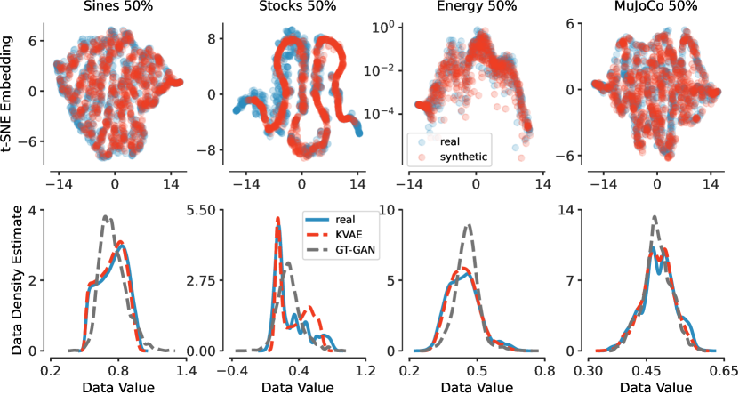
Figure 2: We qualitatively evaluate our approach with two-dimensional t-SNE plots of the synthetic and real data (top row). In addition, we show the PDFs of the real data, and for KVAE and GT-GAN synthetic distributions (bottom row).

\begin{overpic}[width=433.62pt]{figures/constrained_gen_vis_tsne_hist_rev} \put(0.0,27.0){A} \put(24.0,27.0){B} \put(50.0,27.0){C} \put(74.0,27.0){D} \end{overpic}

Figure 3: The t-SNE plots of KVAE with $\beta=0$ (A), KVAE (B), and constrained KVAE (C), and their PDFs (D) are compared to the true nonlinear pendulum data.

5.3 Physics-Constrained Generation

Here, we demonstrate how to incorporate prior knowledge of the problem when generating TS information. While we could study the Sines dataset, we opted for a more challenging test case, the nonlinear pendulum system. Let $l=1$ and $g=9.8$ denote the length and gravity, respectively. Then, we consider the following ordinary differential equation (ODE) that describes the evolution of the angular displacement from an equilibrium $\theta$,

$$\frac{\operatorname*{d}^{2}\theta}{\operatorname*{d}t^{2}}+\frac{g}{l}\sin\theta=0\ ,\quad\theta(0)=0\ ,\quad\dot{\theta}(0)=0\ .$$ (10)

To generate $N$ different sequences, we uniformly sample $\theta^{j}(0)\sim\mathcal{U}(0.5,2.7)$ for $j=1,\dots,N$ over the time interval $t=\left[0,17\right]$, where the time step is defined by $\Delta t=0.1$. This results in a set $\{x_{1:T}^{j}\}_{j=1}^{N}$ with $T=170$ and each time sample is two-dimensional, i.e., $x_{t}\in\mathbb{R}^{2}$. To simulate real-world noisy sensors, we incorporate additive Gaussian noise to each sample. Namely, we sample $\rho\sim\mathcal{N}(0,1)$, and we define the train set samples via $\bar{x}_{t}:=x_{t}+0.08\,\rho$.

We evaluate the nonlinear pendulum on three different models: (i) a VAE; (ii) a KVAE; and (iii) a KVAE with an eigenvalue constraint as described in Sec. 4.3. We visualize in Fig. 3 the t-SNE plots of the real data in comparison to the data generated using the three trained models, VAE in Fig. 3A, KVAE in Fig. 3B, and constrained KVAE in Fig. 3C. We also plot the PDFs of the three models in Fig. 3D. The results clearly show that the synthetic samples generated with the constrained KVAE (red) better match the distribution and PDF of the true process in comparison to KVAE (green) and KVAE with $\beta=0$ (gray).

5.4 Conditional Generation for Weather Data

Accurate weather data is essential for various applications, such as agriculture, water resource management, and disaster early warning. Generative models can produce synthetic weather data to supplement sparse or incomplete observational datasets. Here, we consider the temperature data (at 2m from surface) from the ERA5 dataset (Hersbach et al., 2020) within the region of California. The selected temperature data consists of 6400 samples representing a $80\times 80$ map, each spanning four months with 120 time steps. We construct a validation set from this data by randomly dropping 20% of the samples. Our model is trained with geospatial coordinates as conditional variables. To support the conditional training and generation, we made two simple modifications: (i) we add a very simple MLP to support spatial embeddings $s$; and (ii) we augment the decoder and prior to support conditional generation: $p(x_{t_{1}:t_{N}}|z_{1:T},s)$ and $p(x_{1:T},y_{1:T},s)=p(y_{1:T}|s)p(x_{1:T}|y_{1:T},s)$. In Fig. 4 (left panel), we show the points of interest with respect to the given monitoring stations, which can be used to condition our model. Fig. 4 (middle panel) demonstrates two real and synthetic samples and the coresponding standard deviation bands. Fig. 4 (right panel) compares the real and synthetic density distributions. Remarkably, we show that our model generates a four-month signal that resembles the ground truth for unseen geospatial coordinates. Our results emphasize the ability of our KVAE to generate real-world scientific data. Additional details and results are presented in App. F.

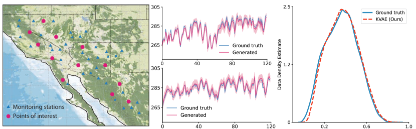
Figure 4: The left panel illustrates the idea of conditional generative models for weather data synthesis at locations of interest. The middle panel presents two representative samples from conditional generations. The standard deviation bands faithfully capture the ground truth data. The right figure shows the general performance of our model using density estimation.

5.5 Ablation Study

We ablate our approach on the discriminative task in the regular and $30\%$ and $50\%$ irregular settings. We eliminate the linear prior by fixing $\beta=0$, and we also train another baseline without the linear prior and without the recurrent (GRU) component. Tab. 4 details our ablation results. We observe that KVAE outperforms all other regular ablation baselines and the majority of irregular baselines. We conclude that by introducing a novel linear variational prior, KVAE improves generative results.

Table 4: Discriminative ablation results with regular and irregular $30\%$ and $50\%$ data on our method (KVAE), without the linear prior ($\beta=0$), and also without the RNN ($\beta=0$, no RNN).

	regular				30%				50%
	Sines	Stocks	Energy	MuJoCo	Sines	Stocks	Energy	MuJoCo	Sines	Stocks	Energy	MuJoCo
KVAE	0.005	0.009	0.143	0.076	0.035	0.162	0.280	0.123	0.030	0.092	0.298	0.117
$\beta=0$	0.006	0.023	0.155	0.087	0.038	0.172	0.295	0.131	0.040	0.181	0.306	0.108
$\beta=0$, no GRU	-	-	-	-	0.268	0.272	0.436	0.267	0.275	0.225	0.444	0.305

6 Conclusion

Generative modeling of TS data is often modeled with GANs which are unstable to train and exhibit mode collpase. In contrast, VAEs are more robust to such issues, but current generative TS approaches employ non-sequential prior models. Further, introducing constraints that impose domain knowledge is challenging in these frameworks. To improve these issues, we propose Koopman VAE (KVAE), a new variational autoencoder that is based on a novel dynamical linear prior. Our method enjoys the benefits of VAEs, it supports regular and irregular TS data, and it faciliates the incorporation of physics-constraints and analysis through the lens of linear dynamical systems theory. We extensively evaluate our approach on generative benchmarks in comparison to strong baselines, and we show that KVAE significantly outperforms existing work on several quantitative and qualitative metrics. We also demonstrate on a real-world challenging climate dataset that KVAE approximates well the associated density distribution and it generates accurate temperature long-term signals. Future work will explore the utility of KVAE for scientific and engineering problems in more depth.

Acknowledgments

OA was partially supported by an ISF grant 668/21, an ISF equipment grant, and by the Israeli Council for Higher Education (CHE) via the Data Science Research Center, Ben-Gurion University of the Negev, Israel. MWM would like to acknowledge NSF and ONR for providing partial support of this work. NBE would like to acknowledge NSF, under Grant No. 2319621, and the U.S. Department of Energy, under Contract Number DE-AC02-05CH11231, for providing partial support of this work. Our conclusions do not necessarily reflect the position or the policy of our sponsors, and no official endorsement should be inferred.

Appendix A Koopman theory and practice

The underlying theoretical justification for our work is related to dynamical systems and Koopman theory (Koopman, 1931). Let $\mathcal{M}\subset\mathbb{R}^{m}$ be a finite-dimensional domain and $\varphi:\mathcal{M}\rightarrow\mathcal{M}$ be a dynamical system defined by

$$x_{t+1}=\varphi(x_{t})\ ,$$

where $x_{t}\in\mathcal{M}$, and $t\in\mathbb{N}$ is a discrete variable that represents time. Remarkably, under some mild conditions (Eisner et al., 2015), there exists an infinite-dimensional operator known as the Koopman operator $\mathcal{K}_{\varphi}$ that acts on observable functions $f:\mathcal{M}\rightarrow\mathbb{C}\subset\mathcal{F}$ and it fully characterizes the dynamics. The operator $\mathcal{K}_{\varphi}$ is given by

$$\mathcal{K}_{\varphi}f(x_{t})=f\circ\varphi(x_{t})\ ,$$

where $f\circ\varphi$ denotes composition of transformations. Remarkably, $\mathcal{K}_{\varphi}$ is linear, while $\varphi$ may be nonlinear. There is an infinitesimal version of $\mathcal{K}_{\varphi}$, known as the Koopman generator (Lasota & Mackey, 1998; Klus et al., 2020), allowing to model the instanteous map of dynamical systems (Azencot et al., 2013; Peitz et al., 2020; Azencot et al., 2021). Further, if the eigendecomposition of the Koopman operator exists, one can discuss the dynamical interpretation of the corresponding eigenvalues and eigenvectors. Spectral analysis of Koopman operators is currently still being researched (Mezić, 2013; Arbabi & Mezic, 2017; Mezic, 2017; Das & Giannakis, 2019). For instance, eigenfunctions whose eigenvalues lie within the unit circle are related to global stability (Mauroy & Mezić, 2016), and to orbits of the system (Mauroy & Mezić, 2013). In practice, several methods have been devised to approximate the Koopman operator, of which the dynamic mode decomposition (DMD) (Schmid, 2010) is perhaps the most well-known technique (Rowley et al., 2009). In this context, our work employs a learnable module akin to DMD in the model prior of our KVAE. Thus, given this discussion, our approach can be viewed as treating the input data as states $x_{1:T}$, and the learnable linear dynamics we compute in KVAE as parametrized by a the latent observable functional space $\mathcal{F}$.

Appendix B Static Variational Autoencoders.

We recall a few governing equations from (Kingma & Welling, 2014; Doersch, 2016). We want to compute the PDF $P(x)$ using a maximum likelihood framework. The density $P(x)$ reads

$$P(x)=\int p(x|z;\theta)p(z)\operatorname*{d}z\ ,$$ (11)

where $z$ is a latent representation associated with $x$. The model $p(x|z;\theta)$ ideally approaches $x$ for some $z$. In variational inference, we typically have that $p(x|z;\theta)=\mathcal{N}(x|f(z;\theta),\sigma^{2}I)$, i.e., a Gaussian distribution where the mean is generated with a neural network $f$. However, two issues arise with the above PDF: 1) how to define $z$; and 2) how to integrate over $z$.

VAEs provide a solution for both issues. The first issue is resolved by assuming that $z$ is drawn from a predefined distribution, e.g., $\mathcal{N}(0,I)$. The second issue can be potentially solved by approximating Eq. 11 with a sum, i.e., $P(x)\approx\frac{1}{n}\sum_{i}p(x|z_{i})$. A challenge, however, is that $n$ needs to be huge in high-dimensions. Instead, we observe that for most $z$, the term $p(x|z)$ will be nearly zero, and thus we can focus on sampling $z$ that are likely to produce $x$. Consequently, we need an approximate posterior $q(z|x)$ which allows to compute $\mathbb{E}_{z\sim q}p(x|z)$, where $z$ is obtained using the re-parametrization trick.

To guide training so that the prior and approximate posterior match, we employ the Kullback–Liebler Divergence $\text{KL}[\cdot\,\|\,\cdot]$ between $q(z)$ and $p(z|x)$. The model is trained using the evidence lower bound (ELBO) loss $\mathbb{E}_{z\sim q}[\log p(x|z)]-\text{KL}[q(z|x)\,\|\,p(z)]$, which is one of the core equations of VAE. Notice that the objective takes the form of reconstruction and regularization penalties, respectively.

Appendix C Neural Controlled Differential Equations

Irregularly sampled TS information $x_{t_{1}:t_{N}}$ for, e.g., $t_{j}\in[1,\dots,T]$ cannot be modeled directly with discrete-time architectures such as recurrent neural networks (RNN). Therefore, the continuous analog of RNN is considered for $x_{t_{1}:t_{N}}$, based on neural controlled differential equations (NCDE) (Kidger et al., 2020) that are given by

$$h(t_{i+1})=h(t_{i})+\int_{t_{i}}^{t_{i+1}}f(h(t)\,;\,\theta_{f})\operatorname*{d}X(t)\ ,$$ (12)

where $h(t_{i})$ is the hidden code associated with $x_{t_{i}}$, $X(t)$ is a continuous-time trajectory generated from $x_{t_{1}:t_{N}}$ via an interpolation method with $X(t_{i}):=x_{t_{i}}$, and $f$ is a neural network parametrized by $\theta_{f}$ whose role is to learn the latent infinitesimal factor.

Appendix D Variational Penalized Evidence Lower Bound

In what follows, we present the derivation of the variational penalized evidence lower bound for our method. Our objective is to minimize $KL[q(z_{\leq T}|x_{\leq T})||p(z_{\leq T}|x_{\leq T})]$ under the Koopman constraint $\mathcal{L}_{\text{pred}}(z_{\leq T},\bar{z}_{\leq T})=\mathbb{E}_{\bar{z}_{\leq T}\sim p}[\log p(z_{\leq T}|\bar{z}_{\leq T})]$. In the following, we change the notations of $y$ and $z$ from the main text, and thus: $p(x_{\leq T},z_{\leq T})=p(z_{\leq T})p(x_{\leq T}|z_{\leq T})$ as in Eq. 1.

$$KL[q(z_{\leq T}|x_{\leq T})||p(z_{\leq T}|x_{\leq T})]+\mathbb{E}_{\bar{z}_{\leq T}\sim p}[\log p(z_{\leq T}|\bar{z}_{\leq T})]$$

$$=\int q(z_{\leq T}|x_{\leq T})\log\frac{q(z_{\leq T}|x_{\leq T})}{p(z_{\leq T}|x_{\leq T})}dz_{\leq T}+\mathbb{E}_{\bar{z}_{\leq T}\sim p}[\log p(z_{\leq T}|\bar{z}_{\leq T})]$$

$$=\int q(z_{\leq T}|x_{\leq T})\log\frac{q(z_{\leq T}|x_{\leq T})p(x_{\leq T})}{p(z_{\leq T},x_{\leq T})}dz_{\leq T}+\mathbb{E}_{\bar{z}_{\leq T}\sim p}[\log p(z_{\leq T}|\bar{z}_{\leq T})]$$

$$=\int q(z_{\leq T}|x_{\leq T})[\log p(x_{\leq T})+\log\frac{q(z_{\leq T}|x_{\leq T})}{p(z_{\leq T},x_{\leq T})}]dz_{\leq T}+\mathbb{E}_{\bar{z}_{\leq T}\sim p}[\log p(z_{\leq T}|\bar{z}_{\leq T})]$$

$$=\log p(x_{\leq T})+\int q(z_{\leq T}|x_{\leq T})\log\frac{q(z_{\leq T}|x_{\leq T})}{p(z_{\leq T},x_{\leq T})}dz_{\leq T}+\mathbb{E}_{\bar{z}_{\leq T}\sim p}[\log p(z_{\leq T}|\bar{z}_{\leq T})]$$

$$=\log p(x_{\leq T})+\int q(z_{\leq T}|x_{\leq T})\log\frac{q(z_{\leq T}|x_{\leq T})}{p(z_{\leq T})p(x_{\leq T}|z_{\leq T})}dz_{\leq T}+\mathbb{E}_{\bar{z}_{\leq T}\sim p}[\log p(z_{\leq T}|\bar{z}_{\leq T})]$$

$$=\log p(x_{\leq T})+\int q(z_{\leq T}|x_{\leq T})[\log\frac{q(z_{\leq T}|x_{\leq T})}{p(z_{\leq T})}-\log p(x_{\leq T}|z_{\leq T})]dz_{\leq T}+\mathbb{E}_{\bar{z}_{\leq T}\sim p}[\log p(z_{\leq T}|\bar{z}_{\leq T})]$$

$$=\log p(x_{\leq T})+\mathbb{E}_{z_{\leq T}\sim q(z_{\leq T}|x_{\leq T})}[\log\frac{q(z_{\leq T}|x_{\leq T})}{p(z_{\leq T})}-\log p(x_{\leq T}|z_{\leq T})]+\mathbb{E}_{\bar{z}_{\leq T}\sim p}[\log p(z_{\leq T}|\bar{z}_{\leq T})]$$

$$=\log p(x_{\leq T})+KL[q(z_{\leq T}|x_{\leq T})||p(z_{\leq T})]-\mathbb{E}_{z_{\leq T}\sim q(z_{\leq T}|x_{\leq T})}[\log p(x_{\leq T}|z_{\leq T})]+\mathbb{E}_{\bar{z}_{\leq T}\sim p}[\log p(z_{\leq T}|\bar{z}_{\leq T})].$$

Thus we have the following:

$$KL[q(z_{\leq T}|x_{\leq T})||p(z_{\leq T}|x_{\leq T})]+\mathbb{E}_{\bar{z}_{\leq T}\sim p}[\log p(z_{\leq T}|\bar{z}_{\leq T})]=$$

$$\log p(x_{\leq T})+KL[q(z_{\leq T}|x_{\leq T})||p(z_{\leq T})]-\mathbb{E}_{z_{\leq T}\sim q(z_{\leq T}|x_{\leq T})}[\log p(x_{\leq T}|z_{\leq T})]+\mathbb{E}_{\bar{z}_{\leq T}\sim p}[\log p(z_{\leq T}|\bar{z}_{\leq T})].$$

Now, rearranging the equation, we yield:

$$\log p(x_{\leq T})-KL[q(z_{\leq T}|x_{\leq T})||p(z_{\leq T}|x_{\leq T})]+\mathbb{E}_{\bar{z}_{\leq T}\sim p}[\log p(z_{\leq T}|\bar{z}_{\leq T})]=$$

$$-\mathbb{E}_{z_{\leq T}\sim q(z_{\leq T}|x_{\leq T})}[\log p(x_{\leq T}|z_{\leq T})]+KL[q(z_{\leq T}|x_{\leq T})||p(z_{\leq T})]+\mathbb{E}_{\bar{z}_{\leq T}\sim p}[\log p(z_{\leq T}|\bar{z}_{\leq T})].$$

Thus finally:

$$\log p(x_{\leq T})+\mathbb{E}_{\bar{z}_{\leq T}\sim p}[\log p(z_{\leq T}|\bar{z}_{\leq T})]\leq$$ (13)

$$-\mathbb{E}_{z_{\leq T}\sim q(z_{\leq T}|x_{\leq T})}[\log p(x_{\leq T}|z_{\leq T})]+KL[q(z_{\leq T}|x_{\leq T})||p(z_{\leq T})]+\mathbb{E}_{\bar{z}_{\leq T}\sim p}[\log p(z_{\leq T}|\bar{z}_{\leq T})].$$

Appendix E Constrained Generation and Analysis

In Section 5.3 we explored the nonlinear pendulum system. We let $l=1$ and $g=9.8$ denote the length and gravity, respectively. Then, we considered the following ordinary differential equation (ODE) that describes the evolution of the angular displacement from an equilibrium $\theta$,

$$\frac{\operatorname*{d}^{2}\theta}{\operatorname*{d}t^{2}}+\frac{g}{l}\sin\theta=0\ ,\quad\theta(0)=0\ ,\quad\dot{\theta}(0)=0\ .$$ (14)

We added noise to our generated samples to make the problem more challenging and interesting. We observed that adding the constraint on the spectrum improves the results, and we were able to get better results than using the vanilla KVAE method. Specifically, we train both models where we fix the latent size $\kappa$ of each $z_{i}$ to be $\kappa=4$. For the constrained version, we additionally add $\mathcal{L}_{\text{eig}}$:

$$\mathcal{L}_{\text{eig}}=||\lambda_{p}|-c_{p}|^{2}+||\lambda_{q}|-c_{q}|^{2}\ ,$$ (15)

where $c_{p}=1,c_{q}=1$ and $\lambda_{p}$ and $\lambda_{q}$ are the largest eigenvalues during training. We define this constraint since the nonlinear pendulum is a stable dynamical system that is governed by two modes. The rest of the eigenvalues, $\lambda_{i}$, where $i\neq p,q$ could be additionally constrained to be equal to zero. However, we observe that when we leave the rest of the eigenvalues to be unconstrained, we get similar behavior. Fig. 5 shows the spectra of the linear operators associated with KVAE and constrained KVAE. We can analyze and interpret the learned dynamics by investigating the spectrum. Specifically, if $|\lambda_{j}|<1$, it is associated with exponentially decaying modes since $\lim_{t\rightarrow\infty}|\lambda_{j}^{t}|=0$. When $|\lambda_{j}|=1$, the associated mode has infinite memory, whereas $|\lambda_{j}|>1$ is associated with unstable behavior of the dynamics, since $\lim_{t\rightarrow\infty}|\lambda_{j}^{t}|=\infty$. In Fig. 5, we observe that training without the constraint results in decaying dynamics where all eigenvalues $\ll$ $1$ (yellow). In contrast, analyzing our approximate operator reveals that as expected, $|\lambda_{p}|$ and $|\lambda_{q}|$ (purple) are approximately one, indicating stable dynamics and the rest (yellow) are approximately zero, as desired.

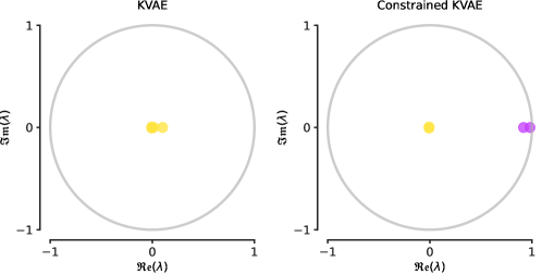
Figure 5: On the left, we show the spectrum of the approximate Koopman operator without constraints during the training. On the right, we show the spectrum of the approximate Koopman operator for the model that is trained with stability constraints. We can see that, indeed, the absolute value of two eigenvalues is approximately 1.

In addition to the analysis of the constrained system in Eq. 14, we also compute the approximate Koopman operators for all the regular systems we consider in the main text. Specifically, we show in Fig. 6 four panels, corresponding to the spectral eigenvalue plots for Sines (left), Stocks (middle left), Energy (middle right), and MuJoCo (right). Green eigenvalues are within the unit circle, whereas red eigenvalues are located outside the unit circle. Noticeably, the learned dynamics for Sines, Stocks and MuJoCo are stable, i.e., their corresponding eigenvalues are within the unit circle. Thus, their training, inference and overall long-term behavior are expected to be numerically stable and not produce values that present large deviations. In contrast, the spectrum associated with the model learned for the Energy dataset reveals unstable dynamics, where the largest $\lambda_{i}$ $\gg$ $1$. We hypothesize that we can benefit from incorporating spectral constraints to regularize the dynamics and achieve stable dynamics. In the future, we will investigate whether spectral constraints can enhance the generation results and overall behavior of such models.

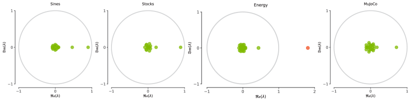
Figure 6: The spectral distribution of the approximate Koopman operator of the prior for each dataset in the regular setting.

Appendix F Conditional Generation Results for Weather Data

Weather forecasting and climate modeling are crucial in agriculture, energy, and disaster management. However, due to the limited availability of weather stations, scientists are faced with the challenge of the inherent sparsity of observational weather data, especially in specific geographical areas of interest. Here, we explore the potential of our KVAE model for modeling temperature dynamics based on sparse measurement data. Our objective is to generate the temperature data at any location within a specific region of interest. Hence, the proposed KVAE model here is conditioned on the geospatial coordinates of the specific region.

We focus on two representative regions in the United States: the California and Central US areas. California has diverse and non-stationary weather changes due to the complex interactions between seas, lands, and mountains. Central US areas present more stable and relatively easier temperature dynamics, compared with the California region. Both of these regions include a grid of $80\times 80$, which means we have 6400 TS samples in total. Moreover, the dataset in this task comprises temperature at 2-meter height above the surface from ERA5 reanalysis dataset (Hersbach et al., 2020). We select 4-month observation data within the specific area for training and evaluating our VAE model. It contains 120 time steps for each TS sample. We split the train and test sets with a ratio of $80\%$ and $20\%$. The generated TS samples are shown in Fig. 10 and Fig. 11. We can see that our KVAE model can accurately capture the underlying dynamics of temperature data in both California and Central US regions. Furthermore, Fig. 7 and Fig. 8 exhibit the comparisons of the temporally-averaged temperature distribution between the generations and ground truth in California and Central US regions. The temperature distribution patterns of the generations align well with those of the ground truth in the entire domain. Similarly, we also observe that the generation and ground truth match well when comparing minimum and maximum values over time, as shown in Fig. 9. Nevertheless, the fine-scale spatial details are lacking in our generation due to the absence of spatial constraints. In the future, we will enhance our conditional KVAE model by incorporating spatial continuity and prior knowledge for spatiotemporal generation.

By leveraging conditional generative models, we hope to provide valuable insights into weather dynamics in specific regions and enhance the decision-making processes that are reliant on accurate weather information.

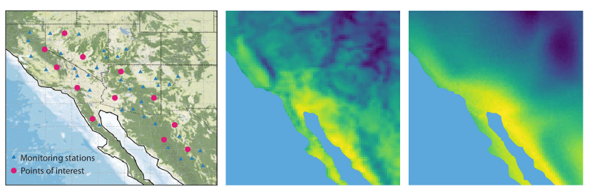
Figure 7: Comparison of the temporally-averaged temperature distribution of the generated signals and ground truth data in California region. left: California region map. middle: ground truth average. right: generated average.

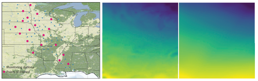
Figure 8: Comparison of the temporally-averaged temperature distribution between the generations and ground truth in Central US region. left: Central US region map. middle: ground truth average. right: generated average.

Appendix G Additional Generation Results

For brevity, in the main text, we provided tables without standard deviation (std). In this section, we provide extended tables that include the std for each metric. Tab. 6 and Tab. 7 present the results for the regular observed data of discriminative and predictive scores, respectively. In Tab. 8, Tab. 9, and Tab. 10 we show the results for the irregular sampled of 30%, 50%, and 70% missing observation, respectively. Each table includes both discriminative and predictive scores. Furthermore, we provide qualitative results to compare our model with GT-GAN, the second-best generation model for both regularly and irregularly sampled data. In Fig. 12, Fig. 13, and Fig. 14, we visualize the t-SNE projection of both ground truth data and generated data (first row) and the PDF of ground truth data versus generated data (second row). We perform the visualization for all regularly and irregularly sampled datasets.

\begin{overpic}[width=433.62pt]{figures/climate_minmax.pdf} \put(0.0,48.0){{\color[rgb]{1,1,1}A}} \put(25.0,48.0){{\color[rgb]{1,1,1}B}} \put(51.0,48.0){{\color[rgb]{1,1,1}E}} \put(76.0,48.0){{\color[rgb]{1,1,1}F}} \put(0.0,22.5){{\color[rgb]{1,1,1}C}} \put(25.0,22.5){{\color[rgb]{1,1,1}D}} \put(51.0,22.5){{\color[rgb]{1,1,1}G}} \put(76.0,22.5){{\color[rgb]{1,1,1}H}} \end{overpic}

Figure 9: The maximum and minimum plots for both California and Central US regions. (A) The maximum value over time of the ground truth in the California region. (B) The maximum value over time of the generation in the California region. (C) The maximum value over time of the ground truth in the Central US region. (D) The maximum value over time of the generation in the Central US region. (E) The minimum value over time of the ground truth in the California region. (F) The minimum value over time of the generation in the California region. (G) The minimum value over time of the ground truth in the Central US region. (H) The minimum value over time of the generation in the Central US region.

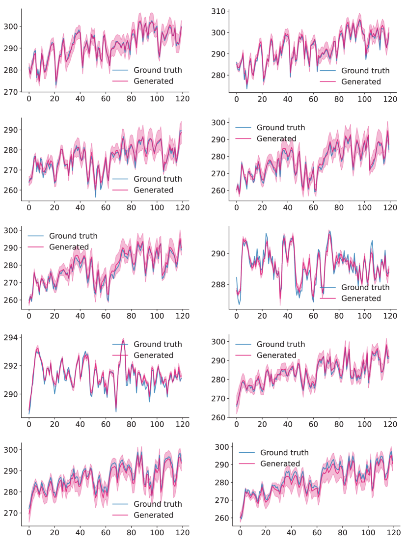
Figure 10: The representative generations in the California area.

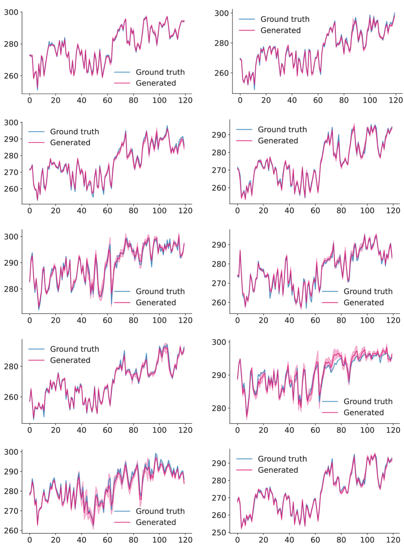
Figure 11: The representative generations in the Central US area.

Method	Copm.	Sines	Stocks	Energy	MuJoCo
KVAE (Ours)	# Parameters	32,929	33,410	230,860	195,902
	Wall Clock Time	2h 49m	2h 49m	5h 16m	3h 46m
GT-GAN	# Parameters	41,913	41,776	57,104	47,346
	Wall Clock Time	10h 12m	12h 20m	10h 39m	13h 12m

Table 5: Comparison of number (#) of parameters and wall clock time.

Appendix H Computational Resources

Here, we compare the model complexity (number of parameters), and the wall clock time measurement with GT-GAN. We present the details in Tab. 5. Both models were trained on the same software and hardware for fair comparison. The software environments we use are: CentOS Linux 7 (Core) and PYTHON 3.9.16; and the hardware is: NVIDIA RTX 3090. We observe that we use more parameters on the Energy and MuJoCo datasets, but the training time is significantly faster on the same software and hardware.

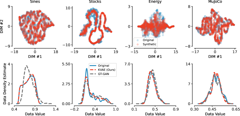
Figure 12: We qualitatively evaluate our approach on regularly sampled data with two-dimensional t-SNE plots of the synthetic and real data (top row). In addition, we show the PDFs of the real data, and for KVAE and GT-GAN synthetic distributions (bottom row).

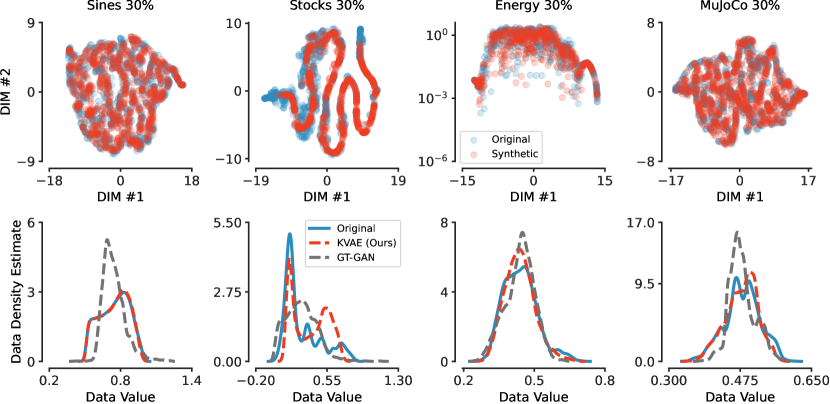
Figure 13: We qualitatively evaluate our approach on 30% irregularly sampled data with two-dimensional t-SNE plots of the synthetic and real data (top row). In addition, we show the PDFs of the real data, and for KVAE and GT-GAN synthetic distributions (bottom row).

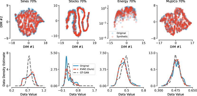
Figure 14: We qualitatively evaluate our approach on 70% irregularly sampled data with two-dimensional t-SNE plots of the synthetic and real data (top row). In addition, we show the PDFs of the real data, and for KVAE and GT-GAN synthetic distributions (bottom row).

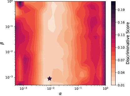
Figure 15: Each point in this plot represents the discriminative score for stocks regularly sampled data set when trained with specific $\alpha$ and $\beta$ values. The star marker denotes the best discriminative score for some $\alpha=9\mathrm{e}{-3},\beta=9\mathrm{e}{-4}$ values. In addition, most of the values in the figure present better performance than the second-best method.

Table 6: Regular TS, discriminative task

Method	Sines	Stocks	Energy	MuJoCo
KVAE (Ours)	.005$\pm$.003	.009$\pm$.006	.143$\pm$.011	.076$\pm$.017
GT-GAN	.012$\pm$.014	.077$\pm$.031	.221$\pm$.068	.245$\pm$.029
TimeGAN	.011$\pm$.008	.102$\pm$.021	.236$\pm$.012	.409$\pm$.028
TimeVAE	.016$\pm$.010	.036$\pm$.033	.323$\pm$.029	.224$\pm$.026
CR-VAE	.342$\pm$.157	.320$\pm$.095	.475$\pm$.054	.464$\pm$.012
RCGAN	.022$\pm$.008	.196$\pm$.027	.336$\pm$.017	.436$\pm$.012
C-RNN-GAN	.229$\pm$.040	.399$\pm$.028	.499$\pm$.001	.412$\pm$.095
T-Forcing	.495$\pm$.001	.226$\pm$.035	.483$\pm$.004	.499$\pm$.000
P-Forcing	.430$\pm$.227	.257$\pm$.026	.412$\pm$.006	.500$\pm$.000
WaveNet	.158$\pm$.011	.232$\pm$.028	.397$\pm$.010	.385$\pm$.025
WaveGAN	.277$\pm$.013	.217$\pm$.022	.363$\pm$.012	.357$\pm$.017
RI	54.54%	75.00%	35.29%	66.07%

Table 7: Regular TS, predictive task

Method	Sines	Stocks	Energy	MuJoCo
KVAE (Ours)	.093$\pm$.000	.037$\pm$.000	.251$\pm$.000	.038$\pm$.002
GT-GAN	.097$\pm$.000	.040$\pm$.000	.312$\pm$.002	.055$\pm$.000
TimeVAE	.093$\pm$.000	.037$\pm$.033	.254$\pm$.000	.039$\pm$.002
TimeGAN	.093$\pm$.019	.038$\pm$.001	.273$\pm$.004	.082$\pm$.006
CR-VAE	.143$\pm$.002	.076$\pm$.013	.277$\pm$.001	.050$\pm$.000
RCGAN	.097$\pm$.001	.040$\pm$.001	.292$\pm$.005	.081$\pm$.003
C-RNN-GAN	.127$\pm$.004	.038$\pm$.000	.483$\pm$.005	.055$\pm$.004
T-Forcing	.150$\pm$.022	.038$\pm$.001	.315$\pm$.005	.142$\pm$.014
P-Forcing	.116$\pm$.004	.043$\pm$.001	.303$\pm$.006	.102$\pm$.013
WaveNet	.117$\pm$.008	.042$\pm$.001	.311$\pm$.005	.333$\pm$.004
WaveGAN	.134$\pm$.013	.041$\pm$.001	.307$\pm$.007	.324$\pm$.006
Original	0.094	0.036	0.250	0.031

Table 8: Irregular TS (30% dropped)

	Method		Sines	Stocks	Energy	MuJoCo
Discriminative Score	VKAE (Ours)		.035$\pm$.023	.162$\pm$.068	.280$\pm$.018	.123$\pm$.018
	GT-GAN		.363$\pm$.063	.251$\pm$.097	.333$\pm$.063	.249$\pm$.035
		TimeGAN-$\bigtriangleup t$	.494$\pm$.012	.463$\pm$.020	.448$\pm$.027	.471$\pm$.016
		RCGAN-$\bigtriangleup t$	.499$\pm$.000	.436$\pm$.064	.500$\pm$.000	.500$\pm$.000
		C-RNN-GAN -$\bigtriangleup t$	.500$\pm$.000	.500$\pm$.001	.500$\pm$.000	.500$\pm$.000
		T-Forcing-$\bigtriangleup t$	.395$\pm$.063	.305$\pm$.002	.477$\pm$.011	.348$\pm$.041
		P-Forcing-$\bigtriangleup t$	.344$\pm$.127	.341$\pm$.035	.500$\pm$.000	.493$\pm$.010
		TimeGAN-D	.496$\pm$.008	.411$\pm$.040	.479$\pm$.010	.463$\pm$.025
		RCGAN-D	.500$\pm$.000	.500$\pm$.000	.500$\pm$.000	.500$\pm$.000
		C-RNN-GAN-D	.500$\pm$.000	.500$\pm$.000	.500$\pm$.000	.500$\pm$.000
		T-Forcing-D	.408$\pm$.087	.409$\pm$.051	.347$\pm$.046	.494$\pm$.004
		P-Forcing-D	.500$\pm$.000	.480$\pm$.060	.491$\pm$.020	.500$\pm$.000
Predictive Score	KVAE (Ours)		.074$\pm$.005	.019$\pm$.001	.049$\pm$.002	.043$\pm$.000
	GT-GAN		.099$\pm$.004	.021$\pm$.003	.066$\pm$.001	.048$\pm$.001
		TimeGAN-$\bigtriangleup t$	.145$\pm$.025	.087$\pm$.001	.375$\pm$.011	.118$\pm$.032
		RCGAN-$\bigtriangleup t$	.144$\pm$.028	.181$\pm$.014	.351$\pm$.056	.433$\pm$.021
		C-RNN-GAN-$\bigtriangleup t$	.754$\pm$.000	.091$\pm$.007	.500$\pm$.000	.447$\pm$.000
		T-Forcing-$\bigtriangleup t$	.116$\pm$.002	.070$\pm$.013	.251$\pm$.000	.056$\pm$.001
		P-Forcing-$\bigtriangleup t$	.102$\pm$.002	.083$\pm$.018	.255$\pm$.001	.089$\pm$.011
		TimeGAN-D	.192$\pm$.082	.105$\pm$.053	.248$\pm$.024	.098$\pm$.006
		RCGAN-D	.388$\pm$.113	.523$\pm$.020	.409$\pm$.020	.361$\pm$.073
		C-RNN-GAN-D	.664$\pm$.001	.345$\pm$.002	.440$\pm$.000	.457$\pm$.001
		T-Forcing-D	.100$\pm$.002	.027$\pm$.002	.090$\pm$.001	.100$\pm$.001
		P-Forcing-D	.154$\pm$.004	.079$\pm$.008	.147$\pm$.001	.173$\pm$.002
	Original**		.071$\pm$.004	.011$\pm$.002	.045$\pm$.001	.041$\pm$.002

Table 9: Irregular TS (50% dropped)

	Method		Sines	Stocks	Energy	MuJoCo
Discriminative Score	KVAE (Ours)		.030$\pm$.017	.092$\pm$.075	.298$\pm$.013	.117$\pm$.019
	GT-GAN		.372$\pm$.128	.265$\pm$.073	.317$\pm$.010	.270$\pm$.016
		TimeGAN-$\bigtriangleup t$	.496$\pm$.008	.487$\pm$.019	.479$\pm$.020	.483$\pm$.023
		RCGAN-$\bigtriangleup t$	.406$\pm$.165	.478$\pm$.049	.500$\pm$.000	.500$\pm$.000
		C-RNN-GAN-$\bigtriangleup t$	.500$\pm$.000	.500$\pm$.000	.500$\pm$.000	.500$\pm$.000
		T-Forcing -$\bigtriangleup t$	.408$\pm$.137	.308$\pm$.010	.478$\pm$.011	.486$\pm$.005
		P-Forcing-$\bigtriangleup t$	.428$\pm$.044	.388$\pm$.026	.498$\pm$.005	.491$\pm$.012
		TimeGAN-D	.500$\pm$.000	.477$\pm$.021	.473$\pm$.015	.500$\pm$.000
		RCGAN-D	.500$\pm$.000	.500$\pm$.000	.500$\pm$.000	.500$\pm$.000
		C-RNN-GAN-D	.500$\pm$.000	.500$\pm$.000	.500$\pm$.000	.500$\pm$.000
		T-Forcing-D	.430$\pm$.101	.407$\pm$.034	.376$\pm$.046	.498$\pm$.001
		P-Forcing-D	.499$\pm$.000	.500$\pm$.000	.500$\pm$.000	.500$\pm$.000
Predictive Score	KVAE (Ours)		.072$\pm$.002	.019$\pm$.001	.049$\pm$.001	.042$\pm$.001
	GT-GAN		.101$\pm$.010	.018$\pm$.002	.064$\pm$.001	.056$\pm$.003
		TimeGAN-$\bigtriangleup t$	.123$\pm$.040	.058$\pm$.003	.501$\pm$.008	.402 $\pm$.021
		RCGAN-$\bigtriangleup t$	.142$\pm$.005	.094$\pm$.013	.391$\pm$.014	.277$\pm$.061
		C-RNN-GAN-$\bigtriangleup t$	.741$\pm$.026	.089$\pm$.001	.500$\pm$.000	.448$\pm$.001
		T-Forcing-$\bigtriangleup t$	.379$\pm$.029	.075$\pm$.032	.251$\pm$.000	.069$\pm$.002
		P-Forcing-$\bigtriangleup t$	.120$\pm$.005	.067$\pm$.014	.263$\pm$.003	.189$\pm$.026
		TimeGAN-D	.169$\pm$.074	.254$\pm$.047	.339$\pm$.029	.375$\pm$.011
		RCGAN-D	.519$\pm$.046	.333$\pm$.044	.250$\pm$.010	.314$\pm$.023
		C-RNN-GAN-D	.754$\pm$.000	.273$\pm$.000	.438$\pm$.000	.479$\pm$.000
		T-Forcing-D	.104$\pm$.001	.038$\pm$.003	.090$\pm$.000	.113$\pm$.001
		P-Forcing-D	.190$\pm$.002	.089$\pm$.010	.198$\pm$.005	.207$\pm$.008
	Original		.071$\pm$.004	.011$\pm$.002	.045$\pm$.001	.041$\pm$.002

Table 10: Irregular TS (70% dropped)

	Method		Sines	Stocks	Energy	MuJoCo
Discriminative Score	KVAE (Ours)		.065$\pm$.012	.101$\pm$.040	.392$\pm$.004	0.119$\pm$.014
	GT-GAN		.278$\pm$.022	.230$\pm$.053	.325$\pm$.047	.275$\pm$.023
		TimeGAN-$\bigtriangleup t$	.500$\pm$.000	.488$\pm$.009	.496$\pm$.008	.494$\pm$.009
		RCGAN-$\bigtriangleup t$	.433$\pm$.142	.381$\pm$.086	.500$\pm$.000	.500$\pm$.000
		C-RNN-GAN-$\bigtriangleup t$	.500$\pm$.000	.500$\pm$.000	.500$\pm$.000	.500$\pm$.000
		T-Forcing-$\bigtriangleup t$	.374$\pm$.087	.365$\pm$.027	.468$\pm$.008	.428$\pm$.022
		P-Forcing-$\bigtriangleup t$	.288$\pm$.047	.317$\pm$.019	.500$\pm$.000	.498$\pm$.003
		TimeGAN-D	.498$\pm$.006	.485$\pm$.022	.500$\pm$.000	.492$\pm$.009
		RCGAN-D	.500$\pm$.000	.500$\pm$.000	.500$\pm$.000	.500$\pm$.000
		C-RNN-GAN-D	.500$\pm$.000	.500$\pm$.000	.500$\pm$.000	.500$\pm$.000
		T-Forcing-D	.436$\pm$.067	.404$\pm$.068	.336$\pm$.032	.493$\pm$.005
		P-Forcing-D	.500$\pm$.000	.449$\pm$.150	.494$\pm$.011	.499$\pm$.000
Predictive Score	KVAE (Ours)		.076$\pm$.004	.012$\pm$.000	.052$\pm$.001	.044$\pm$.001
	GT-GAN		.088$\pm$.005	.020$\pm$.005	.076$\pm$.001	.051$\pm$.001
		TimeGAN-$\bigtriangleup t$	.734$\pm$.000	.072$\pm$.000	.496$\pm$.000	.442$\pm$.000
		RCGAN-$\bigtriangleup t$	.218$\pm$.072	.155$\pm$.009	.498$\pm$.000	.222$\pm$.041
		C-RNN-GAN-$\bigtriangleup t$	.751$\pm$.014	.084$\pm$.002	.500$\pm$.000	.448$\pm$.001
		T-Forcing-$\bigtriangleup t$	.113$\pm$.001	.070$\pm$.022	.251$\pm$.000	.053$\pm$.002
		P-Forcing-$\bigtriangleup t$	.123$\pm$.004	.050$\pm$.002	.285$\pm$.006	.117$\pm$.034
		TimeGAN-D	.752$\pm$.001	.228$\pm$.000	.443$\pm$.000	.372$\pm$.089
		RCGAN-D	.404$\pm$.034	.441$\pm$.045	.349$\pm$.027	.420$\pm$.056
		C-RNN-GAN-D	.632$\pm$.001	.281$\pm$.019	.436$\pm$.000	.479$\pm$.001
		T-Forcing-D	.102$\pm$.001	.031$\pm$.002	.091$\pm$.000	.114$\pm$.003
		P-Forcing-D	.278$\pm$.045	.107$\pm$.009	.193$\pm$.006	.191$\pm$.005
	Original		.071$\pm$.004	.011$\pm$.002	.045$\pm$.001	.041$\pm$.002

Appendix I Hyperparameters Robustness

We also explore how stable our model is to hyperparameter choice. To this end, we perform an extensive grid search over the following space for:

$$\alpha,\beta\in \{1.0,0.9,0.7,0.5,0.3,0.1,0.09,0.07,0.05,0.03,0.01,$$

$$0.009,0.007,0.005,0.003,0.001,0.0009,0.0007,0.0005\}^{2}$$

for the stocks dataset. Fig. 15 shows the discriminative score for each combination of $\alpha$ and $\beta$. Most of the values are lower than the second-best model for this task.

References

- Alaa et al. (2020) Ahmed Alaa, Alex James Chan, and Mihaela van der Schaar. Generative time-series modeling with Fourier flows. In International Conference on Learning Representations, 2020.
- Ang et al. (2023) Yihao Ang, Qiang Huang, Yifan Bao, Anthony KH Tung, and Zhiyong Huang. TSGBench: time series generation benchmark. arXiv preprint arXiv:2309.03755, 2023.
- Arbabi & Mezic (2017) Hassan Arbabi and Igor Mezic. Ergodic theory, dynamic mode decomposition, and computation of spectral properties of the Koopman operator. SIAM Journal on Applied Dynamical Systems, 16(4):2096–2126, 2017.
- Azencot et al. (2013) Omri Azencot, Mirela Ben-Chen, Frédéric Chazal, and Maks Ovsjanikov. An operator approach to tangent vector field processing. In Computer Graphics Forum, volume 32, pp. 73–82. Wiley Online Library, 2013.
- Azencot et al. (2019) Omri Azencot, Wotao Yin, and Andrea Bertozzi. Consistent dynamic mode decomposition. SIAM Journal on Applied Dynamical Systems, 18(3):1565–1585, 2019.
- Azencot et al. (2020) Omri Azencot, N Benjamin Erichson, Vanessa Lin, and Michael W Mahoney. Forecasting sequential data using consistent Koopman autoencoders. In International Conference on Machine Learning, pp. 475–485. PMLR, 2020.
- Azencot et al. (2021) Omri Azencot, N Benjamin Erichson, Mirela Ben-Chen, and Michael W Mahoney. A differential geometry perspective on orthogonal recurrent models. arXiv preprint arXiv:2102.09589, 2021.
- Berman et al. (2023) Nimrod Berman, Ilan Naiman, and Omri Azencot. Multifactor sequential disentanglement via structured Koopman autoencoders. In The Eleventh International Conference on Learning Representations, ICLR, 2023.
- Brown et al. (2020) Tom Brown, Benjamin Mann, Nick Ryder, Melanie Subbiah, Jared D Kaplan, Prafulla Dhariwal, Arvind Neelakantan, Pranav Shyam, Girish Sastry, Amanda Askell, et al. Language models are few-shot learners. Advances in neural information processing systems, 33:1877–1901, 2020.
- Brunton et al. (2021) Steven L Brunton, Marko Budišić, Eurika Kaiser, and J Nathan Kutz. Modern Koopman theory for dynamical systems. SIAM Rev., 2021.
- Budišić et al. (2012) Marko Budišić, Ryan Mohr, and Igor Mezić. Applied Koopmanism. Chaos: An Interdisciplinary Journal of Nonlinear Science, 22(4), 2012.
- Candanedo (2017) Luis Candanedo. Appliances energy prediction. UCI Machine Learning Repository, 2017.
- Che et al. (2018) Zhengping Che, Sanjay Purushotham, Kyunghyun Cho, David Sontag, and Yan Liu. Recurrent neural networks for multivariate time series with missing values. Scientific reports, 8(1):6085, 2018.
- Chen et al. (2018) Ricky TQ Chen, Yulia Rubanova, Jesse Bettencourt, and David K Duvenaud. Neural ordinary differential equations. Advances in neural information processing systems, 31, 2018.
- Cho et al. (2014) Kyunghyun Cho, Bart van Merrienboer, Çaglar Gülçehre, Dzmitry Bahdanau, Fethi Bougares, Holger Schwenk, and Yoshua Bengio. Learning phrase representations using RNN encoder-decoder for statistical machine translation. In Proceedings of the 2014 Conference on Empirical Methods in Natural Language Processing, EMNLP, pp. 1724–1734. ACL, 2014.
- Chung et al. (2015) Junyoung Chung, Kyle Kastner, Laurent Dinh, Kratarth Goel, Aaron C Courville, and Yoshua Bengio. A recurrent latent variable model for sequential data. Advances in neural information processing systems, 28, 2015.
- Coletta et al. (2023) Andrea Coletta, Sriram Gopalakrishan, Daniel Borrajo, and Svitlana Vyetrenko. On the constrained time-series generation problem. arXiv preprint arXiv:2307.01717, 2023.
- Das & Giannakis (2019) Suddhasattwa Das and Dimitrios Giannakis. Delay-coordinate maps and the spectra of Koopman operators. Journal of Statistical Physics, 175(6):1107–1145, 2019.
- Desai et al. (2021) Abhyuday Desai, Cynthia Freeman, Zuhui Wang, and Ian Beaver. TimeVAE: a variational auto-encoder for multivariate time series generation. arXiv preprint arXiv:2111.08095, 2021.
- Doersch (2016) Carl Doersch. Tutorial on variational autoencoders. arXiv preprint arXiv:1606.05908, 2016.
- Dogra & Redman (2020) Akshunna S Dogra and William Redman. Optimizing neural networks via Koopman operator theory. Advances in Neural Information Processing Systems, 33:2087–2097, 2020.
- Donahue et al. (2019) Chris Donahue, Julian McAuley, and Miller Puckette. Adversarial audio synthesis. In International Conference on Learning Representations, 2019.
- Eisner et al. (2015) Tanja Eisner, Bálint Farkas, Markus Haase, and Rainer Nagel. Operator theoretic aspects of ergodic theory, volume 272. Springer, 2015.
- Erichson et al. (2019) N Benjamin Erichson, Michael Muehlebach, and Michael W Mahoney. Physics-informed autoencoders for Lyapunov-stable fluid flow prediction. arXiv preprint arXiv:1905.10866, 2019.
- Esteban et al. (2017) Cristóbal Esteban, Stephanie L Hyland, and Gunnar Rätsch. Real-valued (medical) time series generation with recurrent conditional GANs. arXiv preprint arXiv:1706.02633, 2017.
- Girin et al. (2021) Laurent Girin, Simon Leglaive, Xiaoyu Bie, Julien Diard, Thomas Hueber, and Xavier Alameda-Pineda. Dynamical variational autoencoders: A comprehensive review. Found. Trends Mach. Learn., 15(1-2):1–175, 2021.
- Goodfellow (2016) Ian Goodfellow. Nips 2016 tutorial: Generative adversarial networks. arXiv preprint arXiv:1701.00160, 2016.
- Goodfellow et al. (2014) Ian Goodfellow, Jean Pouget-Abadie, Mehdi Mirza, Bing Xu, David Warde-Farley, Sherjil Ozair, Aaron Courville, and Yoshua Bengio. Generative adversarial networks. Advances in neural information processing systems, 27, 2014.
- Goyal et al. (2016) Anirudh Goyal, Alex Lamb, Ying Zhang, Saizheng Zhang, Aaron C. Courville, and Yoshua Bengio. Professor forcing: a new algorithm for training recurrent networks. In Advances in Neural Information Processing Systems 29, pp. 4601–4609, 2016.
- Graves (2013) Alex Graves. Generating sequences with recurrent neural networks. arXiv preprint arXiv:1308.0850, 2013.
- Han et al. (2022) Minghao Han, Jacob Euler-Rolle, and Robert K. Katzschmann. DeSKO: stability-assured robust control with a deep stochastic Koopman operator. In The Tenth International Conference on Learning Representations, ICLR, 2022.
- Hersbach et al. (2020) Hans Hersbach, Bill Bell, Paul Berrisford, Shoji Hirahara, András Horányi, Joaquín Muñoz-Sabater, Julien Nicolas, Carole Peubey, Raluca Radu, Dinand Schepers, et al. The ERA5 global reanalysis. Quarterly Journal of the Royal Meteorological Society, 146(730):1999–2049, 2020.
- Higgins et al. (2016) Irina Higgins, Loic Matthey, Arka Pal, Christopher Burgess, Xavier Glorot, Matthew Botvinick, Shakir Mohamed, and Alexander Lerchner. beta-VAE: learning basic visual concepts with a constrained variational framework. In International conference on learning representations, 2016.
- Huszár (2017) Ferenc Huszár. Variational inference using implicit distributions. arXiv preprint arXiv:1702.08235, 2017.
- Jarrett et al. (2021) Daniel Jarrett, Ioana Bica, and Mihaela van der Schaar. Time-series generation by contrastive imitation. Advances in Neural Information Processing Systems, 34:28968–28982, 2021.
- Jeon et al. (2022) Jinsung Jeon, Jeonghak Kim, Haryong Song, Seunghyeon Cho, and Noseong Park. GT-GAN: general purpose time series synthesis with generative adversarial networks. Advances in Neural Information Processing Systems, 35:36999–37010, 2022.
- Kidger et al. (2020) Patrick Kidger, James Morrill, James Foster, and Terry Lyons. Neural controlled differential equations for irregular time series. Advances in Neural Information Processing Systems, 33:6696–6707, 2020.
- Kingma & Welling (2014) Diederik P. Kingma and Max Welling. Auto-encoding variational bayes. In 2nd International Conference on Learning Representations, ICLR, 2014.
- Klus et al. (2020) Stefan Klus, Feliks Nüske, Sebastian Peitz, Jan-Hendrik Niemann, Cecilia Clementi, and Christof Schütte. Data-driven approximation of the Koopman generator: Model reduction, system identification, and control. Physica D: Nonlinear Phenomena, 406:132416, 2020.
- Koopman (1931) Bernard O Koopman. Hamiltonian systems and transformation in Hilbert space. Proceedings of the National Academy of Sciences, 17(5):315–318, 1931.
- Lasota & Mackey (1998) Andrzej Lasota and Michael C Mackey. Chaos, fractals, and noise: stochastic aspects of dynamics, volume 97. Springer Science & Business Media, 1998.
- Li et al. (2023) Hongming Li, Shujian Yu, and José C. Príncipe. Causal recurrent variational autoencoder for medical time series generation. In Thirty-Seventh AAAI Conference on Artificial Intelligence, AAAI, pp. 8562–8570, 2023.
- Lucic et al. (2018) Mario Lucic, Karol Kurach, Marcin Michalski, Sylvain Gelly, and Olivier Bousquet. Are GANs created equal? a large-scale study. Advances in neural information processing systems, 31, 2018.
- Lusch et al. (2018) Bethany Lusch, J Nathan Kutz, and Steven L Brunton. Deep learning for universal linear embeddings of nonlinear dynamics. Nature communications, 9(1):4950, 2018.
- Mauroy & Mezić (2013) Alexandre Mauroy and Igor Mezić. A spectral operator-theoretic framework for global stability. In 52nd IEEE Conference on Decision and Control, pp. 5234–5239. IEEE, 2013.
- Mauroy & Mezić (2016) Alexandre Mauroy and Igor Mezić. Global stability analysis using the eigenfunctions of the Koopman operator. IEEE Transactions on Automatic Control, 61(11):3356–3369, 2016.
- Mezić (2013) Igor Mezić. Analysis of fluid flows via spectral properties of the Koopman operator. Annual Review of Fluid Mechanics, 45:357–378, 2013.
- Mezic (2017) Igor Mezic. Koopman operator spectrum and data analysis. arXiv preprint arXiv:1702.07597, 2017.
- Mogren (2016) Olof Mogren. C-RNN-GAN: continuous recurrent neural networks with adversarial training. arXiv preprint arXiv:1611.09904, 2016.
- Morton et al. (2019) Jeremy Morton, Freddie D. Witherden, and Mykel J. Kochenderfer. Deep variational Koopman models: inferring Koopman observations for uncertainty-aware dynamics modeling and control. In Proceedings of the Twenty-Eighth International Joint Conference on Artificial Intelligence, IJCAI, pp. 3173–3179, 2019.
- Naiman & Azencot (2023) Ilan Naiman and Omri Azencot. An operator theoretic approach for analyzing sequence neural networks. In Proceedings of the AAAI conference on artificial intelligence, volume 37, pp. 9268–9276, 2023.
- Orvieto et al. (2023) Antonio Orvieto, Samuel L. Smith, Albert Gu, Anushan Fernando, Çaglar Gülçehre, Razvan Pascanu, and Soham De. Resurrecting recurrent neural networks for long sequences. In International Conference on Machine Learning, ICML, volume 202, pp. 26670–26698, 2023.
- Pan & Duraisamy (2020) Shaowu Pan and Karthik Duraisamy. Physics-informed probabilistic learning of linear embeddings of nonlinear dynamics with guaranteed stability. SIAM Journal on Applied Dynamical Systems, 19(1):480–509, 2020.
- Peitz et al. (2020) Sebastian Peitz, Samuel E Otto, and Clarence W Rowley. Data-driven model predictive control using interpolated Koopman generators. SIAM Journal on Applied Dynamical Systems, 19(3):2162–2193, 2020.
- Ramesh et al. (2022) Aditya Ramesh, Prafulla Dhariwal, Alex Nichol, Casey Chu, and Mark Chen. Hierarchical text-conditional image generation with clip latents. arXiv preprint arXiv:2204.06125, 1(2):3, 2022.
- Redman et al. (2022) William T Redman, Maria Fonoberova, Ryan Mohr, Ioannis G Kevrekidis, and Igor Mezić. An operator theoretic view on pruning deep neural networks. In The Tenth International Conference on Learning Representations, ICLR, 2022.
- Rombach et al. (2022) Robin Rombach, Andreas Blattmann, Dominik Lorenz, Patrick Esser, and Björn Ommer. High-resolution image synthesis with latent diffusion models. In Proceedings of the IEEE/CVF conference on computer vision and pattern recognition, pp. 10684–10695, 2022.
- Rowley et al. (2009) Clarence W Rowley, Igor Mezić, Shervin Bagheri, Philipp Schlatter, and Dan S Henningson. Spectral analysis of nonlinear flows. Journal of fluid mechanics, 641:115–127, 2009.
- Saxena & Cao (2021) Divya Saxena and Jiannong Cao. Generative adversarial networks (GANs) challenges, solutions, and future directions. ACM Computing Surveys (CSUR), 54(3):1–42, 2021.
- Schmid (2010) Peter J Schmid. Dynamic mode decomposition of numerical and experimental data. Journal of fluid mechanics, 656:5–28, 2010.
- Sohl-Dickstein et al. (2015) Jascha Sohl-Dickstein, Eric Weiss, Niru Maheswaranathan, and Surya Ganguli. Deep unsupervised learning using nonequilibrium thermodynamics. In International conference on machine learning, pp. 2256–2265. PMLR, 2015.
- Srinivasan & Takeishi (2020) Anand Srinivasan and Naoya Takeishi. An MCMC method for uncertainty set generation via operator-theoretic metrics. In 59th IEEE Conference on Decision and Control, CDC, pp. 2714–2719, 2020.
- Strogatz (2018) Steven H Strogatz. Nonlinear dynamics and chaos with student solutions manual: With applications to physics, biology, chemistry, and engineering. CRC press, 2018.
- Takeishi et al. (2017) Naoya Takeishi, Yoshinobu Kawahara, and Takehisa Yairi. Learning Koopman invariant subspaces for dynamic mode decomposition. Advances in neural information processing systems, 30, 2017.
- Tayal et al. (2023) Kshitij Tayal, Arvind Renganathan, Rahul Ghosh, Xiaowei Jia, and Vipin Kumar. Koopman invertible autoencoder: Leveraging forward and backward dynamics for temporal modeling. arXiv preprint arXiv:2309.10291, 2023.
- Todorov et al. (2012) Emanuel Todorov, Tom Erez, and Yuval Tassa. MuJoCo: a physics engine for model-based control. In 2012 IEEE/RSJ International Conference on Intelligent Robots and Systems, pp. 5026–5033. IEEE, 2012. doi: 10.1109/IROS.2012.6386109.
- van den Oord et al. (2016) Aäron van den Oord, Sander Dieleman, Heiga Zen, Karen Simonyan, Oriol Vinyals, Alex Graves, Nal Kalchbrenner, Andrew W. Senior, and Koray Kavukcuoglu. WaveNet: a generative model for raw audio. In The 9th ISCA Speech Synthesis Workshop, pp. 125, 2016.
- Van der Maaten & Hinton (2008) Laurens Van der Maaten and Geoffrey Hinton. Visualizing data using t-sne. Journal of machine learning research, 9(11), 2008.
- Wang et al. (2023) Rui Wang, Yihe Dong, Sercan Ö. Arik, and Rose Yu. Koopman neural forecaster for time series with temporal distribution shifts. In The Eleventh International Conference on Learning Representations, ICLR, 2023.
- Xu et al. (2020) Tianlin Xu, Li Kevin Wenliang, Michael Munn, and Beatrice Acciaio. COT-GAN: generating sequential data via causal optimal transport. Advances in neural information processing systems, 33:8798–8809, 2020.
- Yoon et al. (2019) Jinsung Yoon, Daniel Jarrett, and Mihaela Van der Schaar. Time-series generative adversarial networks. Advances in neural information processing systems, 32, 2019.
- Zeng et al. (2023) Ailing Zeng, Muxi Chen, Lei Zhang, and Qiang Xu. Are transformers effective for time series forecasting? In Proceedings of the AAAI conference on artificial intelligence, pp. 11121–11128, 2023.
- Zhou et al. (2023) Linqi Zhou, Michael Poli, Winnie Xu, Stefano Massaroli, and Stefano Ermon. Deep latent state space models for time-series generation. In International Conference on Machine Learning, pp. 42625–42643. PMLR, 2023.