Monitoring the young planet host V1298 Tau with SPIRou: planetary system and blackevolving large-scale magnetic field

Abstract

We report results of a spectropolarimetric monitoring of the young Sun-like star V1298 Tau based on data collected with the near-infrared spectropolarimeter SPIRou at the Canada-France-Hawaii Telescope between late 2019 and early 2023. Using Zeeman-Doppler Imaging and the Time-dependent Imaging of Magnetic Stars methods on circularly polarized spectra, we reconstructed the large-scale magnetic topology of the star (and its temporal evolution), found to be mainly poloidal and axisymmetric with an average strength varying from 90 to 170 G over the $\mathord{\sim}3.5$ years of monitoring. The magnetic field features a dipole whose strength evolves from 85 to 245 G, and whose inclination with respect to the stellar rotation axis remains stable until 2023 where we observe a sudden change, suggesting that the field may undergo a polarity reversal, potentially similar to those periodically experienced by the Sun. Our data suggest that the differential rotation shearing the surface of V1298 Tau is about 1.5 times stronger than that of the Sun. blackWhen coupling our data with previous photometric results from blackK2 and TESS and assuming circular orbits for all four planets, we report a $3.9\sigma$ detection of the radial velocity signature of the outermost planet (e), associated with a blackmost probable mass, density and orbital period of $M_{e}=0.95^{+0.33}_{-0.24}$ M_♃, $\rho_{e}=1.66^{+0.61}_{-0.48}$ $\rm g\,cm^{-3}$ and $P_{e}=53.0039\pm 0.0001$ d, respectively. For the 3 inner planets, we only derive 99% confidence upper limits on their mass of $0.44$ M_♃, $0.22$ M_♃ and $0.25$ M_♃, for b, c and d, respectively.

1 Introduction

The detection and characterization of exoplanets around young Sun-like stars is key for deriving observational constraints on theoretical models of the early phases of star / planet formation. In particular, it is essential to estimate the radii and masses, and thereby the bulk densities, of young planets to refine the mass-radius relations for planets younger than 30 Myr (Mann et al., 2016). In addition, characterizing the orbital configuration of young close-in giants will bring new clues on the inward migration that giant planets are subject to as they form within the protoplanetary discs of their host stars, and thereby on the impact migrating giant planets have on the dynamical architecture of early planetary systems (Baruteau et al., 2014). However, only few such planets have yet been detected, partly due to the high activity levels that Pre-Main Sequence (PMS) stars exhibit, especially due to their short rotation period. Such active stars indeed generate photometric and radial velocity (RV) signatures that are much larger than those expected from transiting planets, even in the case of close-in giant ones. To date, only 9 planets younger than 25 Myr have well-measured radii thanks to the detection of photometric transits whose depths are typically 10 times smaller than the photometric variations caused by activity: the Super-Neptune K2-33 b (David et al., 2016); the two warm Neptunes AU Mic b and c (Plavchan et al., 2020; Martioli et al., 2021; Szabó et al., 2022); the four Jupiter-size planets V1298 Tau b, c, d and e (David et al., 2019b; Feinstein et al., 2022); the hot Jupiter HIP 67522 b (Rizzuto et al., 2020); and the warm Jupiter HD 114082 b (Zakhozhay et al., 2022). Constraining the mass of these planets is important to refine the mass-radius relations at such early stages of evolution but also to better characterize these young planets in terms of density and composition. However, detecting these planets through velocimetric monitoring is still challenging given that the amplitude of the RV fluctuations induced by the star itself can reach more than $\mathord{\sim}10\times$ the amplitude of the planet signatures (e.g. Donati et al. 2023).

This stellar activity is strongly related to the magnetic field hosted by PMS stars. It is therefore essential to characterize the large-scale magnetic field of such stars to better understand the underlying dynamo processes at work in the stellar interior, but also to analyse star-planet interactions (e.g. Strugarek et al. 2015). In particular, Zeeman-Doppler Imaging (ZDI; Semel 1989; Donati et al. 2006), an efficient tomographic method, already allowed one to reconstruct the large-scale magnetic topology of active PMS stars from time series of circularly polarized spectra (e.g. Donati et al. 2016, 2023; Yu et al. 2017, 2019; Finociety et al. 2021, 2023). New tomographic methods, such as Time-dependent Imaging of Magnetic Stars (TIMeS; Finociety & Donati 2022), are under development to take into account the temporal evolution of stellar magnetic fields, which would help to unveil the long-term evolution of the field and to identify whether these stars feature a magnetic cycle or not.

In this paper we focus on V1298 Tau, an early-K post T Tauri star with no reported accretion (David et al., 2019a), known to be the youngest solar-mass star with a multiplanetary system for which the radii of Jupiter-like planets have been precisely measured to date. V1298 Tau is located in the Taurus constellation at a distance of $108.0\pm 0.2$ pc (Gaia Collaboration et al., 2023). blackFrom Gaia measurements, the effective temperature and the logarithmic surface gravity are found to be equal to $T_{\rm eff}=4941_{-16}^{+31}$ K and $\log{g}=4.227_{-0.008}^{+0.010}$ (Gaia Collaboration et al., 2023), respectively, in agreement with previous values derived by Suárez Mascareño et al. (2021) and David et al. (2019a), of $5050\pm 100$ K / $4.25\pm 0.20$ and $4970\pm 120$ K / $4.246\pm 0.034$, respectively. Suárez Mascareño et al. (2021) also outlined that the effective temperature is consistent with that inferred from the $JHK_{S}$ photometry obtained with the two Micron All-Sky Survey (2MASS) and from the Johnson $V$ photometry collected with the AAVSO Photometric All-Sky Survey (APASS) when assuming an extinction $E(B-V)=0.061$, blackcorresponding to an extinction $A_{v}=0.19\pm 0.10$ following the standard extinction law. A previous independent estimate of the color excess from the multicolor Maidanak observations yields consistent value [$E(V-R_{j})=0.06$ and $A_{v}=0.24$ mag; Grankin 2013].

Given the stellar rotation period and the line-of-sight projected equatorial velocity we obtained (Sec. 3.2), one can infer a relatively accurate estimate of the stellar radius, equal to $R_{*}=1.43\pm 0.03$ R_⊙, assuming the stellar rotation axis is perpendicular to the line of sight. Using the Gaia estimate for the $\log{g}$, one therefore infers a stellar mass $M_{*}=1.26\pm 0.06$ M_⊙. blackFrom $T_{\rm eff}$ and $R_{*}$, we also estimate the luminosity relative to the Sun to be equal to $L_{*}/L_{\odot}=1.094\pm 0.050$. Our updated values of the stellar parameters are summarized in Table 1. These estimates are consistent with those previously determined by Suárez Mascareño et al. (2021), equal to $1.170\pm 0.060$ M_⊙, $1.278\pm 0.070$ R_⊙ and $0.954\pm 0.040$, for the mass, radius and relative luminosity, respectively, from absolute magnitudes and evolutionary models. From its position in the temperature-luminosity diagram, using our updated stellar parameters, we find that the age of V1298 Tau is $\mathord{\sim}10$–15 Myr (using the models of Siess et al. 2000 or Baraffe et al. 2015; Fig. 1), making V1298 Tau younger than previously estimated (e.g. David et al. 2019a; Suárez Mascareño et al. 2021). More recent studies focussing on the kinematics of V1298 Tau, based on Gaia DR3, suggest that the star may belong to the D2 (Krolikowski et al., 2021) or D3 (Gaidos et al., 2022) subgroups of the Taurus star forming region, both being younger than 10 Myr. This comes as further argument in favour of V1298 Tau being younger than initially estimated. The evolutionary models of Siess et al. (2000) and Baraffe et al. (2015) also predict that the depth of the convective envelope of V1298 Tau is about 40% of the stellar radius, similar to that of AB Dor ($M_{*}=1$ M_⊙) or LQ Hya ($M_{*}=0.95$ M_⊙), two young solar-mass stars slightly older than V1298 Tau (40 - 50 Myr; Donati et al. 2003a).

Table 1: Stellar properties used in our study.

distance (pc)	$108.0\pm 0.2$	Gaia Collaboration et al. (2023)
$T_{\rm eff}$ (K)	$4941^{+31}_{-16}$	Gaia Collaboration et al. (2023)
$\log g$ (dex)	$4.227^{+0.010}_{-0.008}$	Gaia Collaboration et al. (2023)
$R_{*}$ (R⊙)	black$1.43\pm 0.03$	blackfrom $v\sin{i}$ and $P_{\rm rot}$
$M_{*}$ (M⊙)	black$1.26\pm 0.06$	blackfrom $R_{*}$ and $\log{g}$
$L/L_{\odot}$	$1.094\pm 0.05$	from $T_{\rm eff}$ and $R_{*}$
$P_{\rm rot}$ (d)	2.91	period used to phase data
$P_{\rm rot}$ (d)	$2.910\pm 0.005$	from $B_{\ell}$
$P_{\rm rot}$ (d)	$2.909\pm 0.009$	from RVs
$v\sin{i}$ ($\mathrm{km\,s^{-1}}$)	$24.9\pm 0.5$	from ZDI
$\Omega_{\rm eq}$ ($\rm mrad\,d^{-1}$)	$2185.1\pm 0.5$	from ZDI
d$\Omega$ ($\rm mrad\,d^{-1}$)	$82.0\pm 2.0$	derived from ZDI
age (Myr)	$10\pm 1$	from of Baraffe et al. (2015)
age (Myr)	$14\pm 1$	from of Siess et al. (2000)

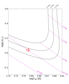
Figure 1: Location of V1298 Tau in the HR diagram, using the updated $T_{\rm eff}$ and $R_{*}$ from Table 1. The black lines correspond to evolutionary tracks from models of Baraffe et al. (2015) for the stellar mass indicated above the curves while isochrones are depicted as magenta dashed lines.

V1298 Tau is a target of great interest to study planetary systems at very early stages of their evolution. In the last few years, many studies therefore focused on this system to further characterize the planet properties. In particular, from transit events observed in the K2 and TESS light-curves, the orbital periods of the three innermost planets (b, c and d) were precisely measured (David et al., 2019b; Feinstein et al., 2022). However, and with only 2 transits reported so far, the orbital period of planet e is less well determined, with black17 possible values ranging from 42.7 to 62.8 d (Feinstein et al., 2022), 7 of them being more plausible, between 43.3 and 55.4 d (Sikora et al., 2023). From velocimetric measurements, Suárez Mascareño et al. (2021) estimated the mass of planets b and e to be equal to $0.64\pm 0.19$ and $1.16\pm 0.30$ M_♃, respectively, while Sikora et al. (2023) found (i) a lower mass for planet e ($0.66\pm 0.26$ M_♃), (ii) only an upper limit for planet b’s mass of 0.50 M_♃ and (iii) a low-significance $2.2\sigma$ blackcandidate detection of planet c with a mass of $0.062^{+0.029}_{-0.028}$ M_♃. A more recent study of Turrini et al. (2023), based on the same RV dataset as in Suárez Mascareño et al. (2021), reports a slightly larger mass for planet e, equal to $1.23^{+0.35}_{-0.48}$ M_♃, more consistent with the estimate of Suárez Mascareño et al. (2021). In addition, the obliquity of the orbital axis of planets b and c with respect to the stellar rotation axis is found to be low, suggesting that these planets underwent a smooth migration inwards within the protoplanetary disc (Feinstein et al., 2021; Gaidos et al., 2022). V1298 Tau also offers the opportunity to study atmospheres of young planets, by measuring or constraining the atmospheric evaporation of the innermost planets resulting from the high activity of the host star (Poppenhaeger et al., 2021; Vissapragada et al., 2021; Maggio et al., 2022).

V1298 Tau has been monitored between late 2019 and early 2023 with the near-infrared (NIR) spectropolarimeter SPIRou in the framework of the SPIRou Legacy Survey (SLS), a large programme allocated 310 nights at blackthe Canada-France-Hawaii Telescope (CFHT), within a PI programme, and most recently, within the SPICE large programme (174 nights blackallocated between late 2022 and mid 2024) at CFHT, aiming at consolidating and enhancing the results provided by the SLS. We start this paper with a detailed description of our spectropolarimetric data set (Sec. 2). We then present the results concerning the large-scale magnetic field of blackV1298 Tau, reconstructed thanks to ZDI and TIMeS (Sec. 3). In Sec. 4, we analyse our velocimetric measurements to constrain the mass of the planets hosted by V1298 Tau and the orbital period of planet e. In Sec. 5, we focus on the stellar activity using three activity proxies in the NIR domain (the He i triplet at 1083 nm and the Paschen $\beta$ and Brackett $\gamma$ lines). We finally summarize and discuss our results in Sec. 6.

2 Observations

We extensively observed V1298 Tau with SPIRou between late 2019 and early 2023, collecting 181 high-resolution spectra ranging from 950 to 2500 nm at a spectral resolving power of $\mathord{\sim}$70,000 (Donati et al., 2020). Altogether, 97 of these observations were collected in the framework of the SLS (2019 Oct 02 - 2021 Jan 08, 2022 Feb 01), more specifically within the WP3 package focusing on the magnetic topology of PMS stars, 52 within the PI Programme of Benjamin Finociety (run ID 21BF21, 2021 Sep 17 - 2022 Jan 30) and the 32 remaining blackones within the SPICE large programme (2022 Nov 02 - 2023 Feb 09). blackMore specifically, the observations are spread over four observing seasons: (i) $\mathord{\sim}140$ d from 2019 Oct to 2020 Feb, (ii) $\mathord{\sim}135$ d from 2020 Aug to 2021 Jan, (iii) $\mathord{\sim}137$ d from 2021 Sep to 2022 Feb; and (iv) $\mathord{\sim}99$ d from 2022 Nov to 2023 Feb. Each observation is composed of a sequence of 4 subexposures of $\mathord{\sim}500$ s taken at different azimuths of the polarimeter retarder in order to get rid of potential spurious signals in the polarization and systematic errors at first order (Donati et al., 1997). We show the journal of observations in Appendix A.

Data reduction was first carried out with a version of the Libre-ESpRIT pipeline, orginally developped for ESPADOnS data (Donati et al., 1997), adapted for SPIRou observations (Donati et al., 2020). In addition, we corrected the spectra from telluric lines using a PCA approach similar to the one developped in Artigau et al. (2014), providing us 176 usable telluric-corrected spectra in both unpolarized (Stokes $I$) and circularly polarized (Stokes $V$) blackobservations, leaving out 5 blackspectra whose quality is too low for our spectropolarimetric analysis black(Table 6). The signal-to-noise ratio (SNR) per pixel in the $H$ band of blackthe usable spectra range from 80 to 253 (median of 212). We then applied Least-Squares Deconvolution (LSD; Donati et al. 1997) on the 176 spectra, using a mask generated with the VALD-3 database (Ryabchikova et al., 2015), featuring an effective temperature and a $\log g$ of 5000 K and 4.5, respectively, and containing moderate to strong atomic lines only (relative depth $>10$% of the continuum). The resulting Stokes $V$ LSD profiles show clear Zeeman signatures whose typical peak-to-peak amplitude is of 0.2%, with SNRs ranging from black1400 to 5700 (median of 4770). blackAs for the other similar young planet-hosting star AU Mic (Donati et al., 2023), we however do not observe clear distorsions of the Stokes $I$ LSD profiles, suggesting that our spectroscopic data are only weakly affected by brightness features at the surface of the star, in agreement with the small amplitude of the photometric fluctuations in the TESS light curve (2021 Sep 16 - Nov 06) of the order of a few percent. We will therefore only focus on the reconstruction of the large-scale magnetic field from our LSD profiles in the following (Sec. 3).

We also processed the 181 observations with the nominal SPIRou pipeline, called APERO (Cook et al., 2022), blackmuch better optimised for RVs than Libre-ESpRIT. Applying the line-by-line (LBL) method (Artigau et al., 2022) on each reduced spectrum yielded 174 accurate RV values, with a blacktypical error bar of 14 $\mathrm{m}\,\mathrm{s}^{-1}$(Table 9). Seven spectra were rejected (on 2019 Dec 08, 2019 Dec 13, 2020 Jan 26, 2020 Jan 27, 2020 Jan 28, 2020 Nov 06 and 2022 Feb 01), affected by instrumental effects and/or bad weather conditions, blackwhich prevented us to obtain accurate blackRVs at these dates.

3 Magnetic field of V1298 Tau

3.1 Longitudinal field

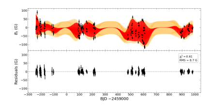
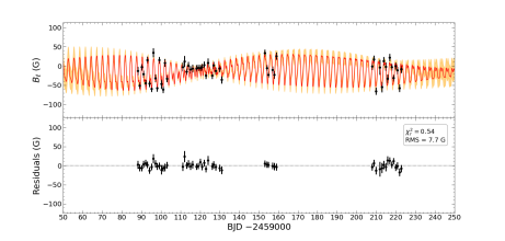
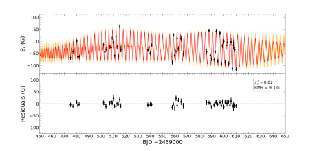
Figure 2: Longitudinal field measurements of V1298 Tau blackobtained from SPIRou data blackover our observing period (top panel) with a zoom on the 2020 Aug - 2021 Jan (middle panel) and 2021 Sep - 2022 Feb (bottom panel) seasons. blackFor each panel, the top plot shows he raw measurements as black dots with their associated error bars while the red curve represents the quasi-periodic GP fit with the 1$\sigma$ confidence area in light orange. The bottom plots show the residuals between the raw measurements and the fit, blackshowing a RMS dispersion of 8.7 G, i.e. smallest than the typical error bar of 9.5 G, and a $\chi^{2}_{r}=0.61$.

We computed the longitudinal field $B_{\ell}$, i.e. the line-of-sight-projected component of the vector magnetic field averaged over the visible hemisphere, as the first moment of our 176 Stokes $V$ LSD profiles (Donati et al., 1997). blackWe find that $B_{\ell}$ ranges from $-115$ to 89 G between 2019 and 2023, with a typical uncertainty of 9.5 G. blackAs we expect $B_{\ell}$ to be rotationally modulated, we modelled these values using a quasi-periodic (QP) Gaussian Process (GP; Rasmussen & Williams 2006), following the definition given by Rajpaul et al. (2015):

$$k(t,t^{\prime})=\theta_{1}^{2}\,\exp\left[-\frac{(t-t^{\prime})^{2}}{2\,\theta_{2}^{2}}-\frac{\sin^{2}\left(\frac{(t-t^{\prime})\pi}{\theta_{3}}\right)}{2\,\theta_{4}^{2}}\right]$$ (1)

where $t$ and $t^{\prime}$ correspond to the dates of two observations. $\theta_{1}$ is the amplitude of the GP, $\theta_{2}$ is the exponential decay time-scale (estimating the typical lifetime of the features generating the signal, e.g. spots), $\theta_{3}$ is the recurrence period (close to the stellar rotation period $P_{\rm rot}$) and $\theta_{4}$ is the smoothing parameter setting the amount of short-term variations included in the fit. We also added another parameter, called $\theta_{5}$, representing a potential excess of uncorrelated noise, not taken into account in our measured error bars (e.g. due to instrinsic variability). We then want to maximize the log likelihood function $\log\mathcal{L}$ defined in Eq. (2) :

$$\log\mathcal{L}=-\frac{1}{2}\left(N_{0}\log{2\pi}+\log{|\boldsymbol{\mathsf{K}}+\boldsymbol{{\Sigma}}+\boldsymbol{\mathsf{S}}|+\boldsymbol{y}^{T}(\boldsymbol{\mathsf{K}}+\boldsymbol{{\Sigma}}+\boldsymbol{\mathsf{S}})^{-1}\boldsymbol{y}}\right)$$ (2)

where $\boldsymbol{y}$ is the vector of the measured $B_{\ell}$, whose length is equal to $N_{0}$ (i.e. to the number of observations). $\boldsymbol{\mathsf{K}}$ corresponds to the covariance matrix associated with the quasi-periodic kernel, $\boldsymbol{{\Sigma}}$ represents a diagonal matrix containing the variance of our measurements and $\boldsymbol{\mathsf{S}}=\theta_{5}^{2}\,\boldsymbol{\mathsf{I}}$ with $\boldsymbol{\mathsf{I}}$ being the identity matrix.

We used a MCMC approach, thanks to the emcee python module (Foreman-Mackey et al., 2013), to explore the parameter domains and sample the posterior distribution of our 5 parameters, based on 20000 iterations of 150 walkers. We then estimated the optimal set of parameters (maximizing $\log\mathcal{L}$) from these posterior distributions (see Table 2), after removing a burn-in period of 5000 iterations.

We find that the recurrence period is well constrained ($\theta_{3}=2.910\pm 0.005$ d) and consistent with the estimate of the stellar rotation period provided by Suárez Mascareño et al. (2021). $B_{\ell}$ data are fitted down to $\chi^{2}_{r}=0.61$, the RMS of the residuals being smaller than the typical error bar (see Fig. 2), suggesting that these data are not significantly affected by intrinsic variability as demonstrated by a value of $\theta_{5}$ smaller than the typical uncertainty and compatible with 0 within $\mathord{\sim}2\sigma$.

As expected by the low value of the decay time-scale, close to one month ($\theta_{2}=36\pm 5$ d, i.e. about 4 times smaller than a typical observing season), we observe a clear evolution of the longitudinal field between blacklate 2019 and early 2023, and within each season. In particular, we note that the full amplitude of the curve has a minimum in 2020 ($\mathord{\sim}30$ G) and a maximum in 2021 ($\mathord{\sim}130$ G). This evolution already indicates that we need to split the dataset of each season into several subsets to apply ZDI that assumes a static configuration of the magnetic topology (Sec. 3.2).

Running GP regression on individual observing season, we find that the decay time-scale is much less constrained and equal to black$68^{+70}_{-35}$ d, $56^{+22}_{-16}$ d, $102^{+59}_{-38}$ d and $41^{+15}_{-11}$ d during 2019 Oct - 2020 Feb, 2020 Aug - 2021 Jan, 2021 Sep - 2022 Feb and 2022 Nov - 2023 Feb, respectively, reflecting a slower evolution of the magnetic field during the 2021-2022 observing season.

Table 2: blackOptimal value obtained for the GP modeling of the longitudinal field $B_{\ell}$ from a MCMC approach. The knee of the modified Jeffreys priors is set to the typical uncertainty on the the longitudinal field, noted $\sigma_{B_{\ell}}$.

Hyperparameter	Prior	Optimal value
GP amplitude (G), $\theta_{1}$	mod Jeffreys ($\sigma_{B_{\ell}}$)	$37\pm 5$
Decay time-scale (d), $\theta_{2}$	Uniform (0, 200)	$36\pm 5$
Recurrence period (d), $\theta_{3}$	Gaussian (2.91, 0.1)	$2.910\pm 0.005$
Smoothing, $\theta_{4}$	Uniform (0,3)	$0.47\pm 0.06$
Uncorrelated noise (G), $\theta_{5}$	mod Jeffreys ($\sigma_{B_{\ell}}$)	$3.2^{+3.4}_{-1.7}$

We note that we were not able to measure the surface field of V1298 Tau, unlike what has been done for the other young star AU Mic, given the large line-of-sight projected equatorial velocity ($v\sin{i}$) value ($\mathord{\sim}25$ $\mathrm{km}\,\mathrm{s}^{-1}$, see Sec. 3.2) that prevented us from obtaining reliable measurements from rotationally broadened unpolarized line profiles.

3.2 Zeeman-Doppler Imaging

In order to reconstruct the large-scale magnetic field of V1298 Tau, we used ZDI (Semel, 1989; Brown et al., 1991; Donati & Brown, 1997; Donati et al., 2006), a tomographic method allowing one to invert Stokes $I$ and $V$ LSD profiles into a large-scale magnetic topology at the surface of an active star. As this problem is ill-posed (infinite number of topologies compatible with the data blackat a given $\chi^{2}_{r}$ level), ZDI uses the principle of maximum entropy to blackselect the simplest solution, i.e. blackthe one with the minimal amount of information needed to fit the data down to blackthe requested $\chi^{2}_{r}$ level, by iteratively adding magnetic features at the surface of the star and comparing the associated LSD profiles with the observed ones.

In practice, we divide the stellar surface into a grid of 3000 cells, initially with no magnetic field. At each iteration, the local Stokes $I$ and/or $V$ LSD profiles are computed from each cell using the Unno-Rachkovsky’s solution of the polarized radiative transfer equations in a plane-parallel Milne Eddington atmosphere (e.g. Landi Degl’Innocenti & Landolfi 2004), and then integrated over the visible stellar hemisphere, providing the synthetic LSD profiles corresponding to the reconstructed image. As mentioned in Finociety et al. (2023), we replaced the built-in prescription for the limb-darkening law by a linear relation for the continuum only, choosing a limb-darkening coefficient $\epsilon=0.3$ compatible with $T_{\rm eff}=5000$ K and $\log g=4.5$ in the $H$ band (Claret & Bloemen, 2011).

The large-scale magnetic field is described by the sum of a poloidal and a toroidal component, both described as spherical harmonic expansions using the formalism of Donati et al. (2006). In particular, the poloidal component is characterized by sets of complex coefficients noted $\alpha_{\ell,m}$ and $\beta_{\ell,m}$ while the toroidal component is fully described by a set of complex coefficients $\gamma_{\ell,m}$, where $\ell$ and $m$ denote the degree and order of the spherical harmonic mode in the expansion. We limited our study to the spherical harmonic modes up to a degree $\ell_{\max}=10$ as adding higher degree modes does not significantly improve the reconstruction.

ZDI also allows one to reconstruct the distribution of dark and bright features at the surface of active stars from distorsions of the Stokes $I$ LSD profiles. blackHowever, we find that, for V1298 Tau, brightness inhomogeneities have only a minor impact on our data (and our reconstructed magnetic maps) as only very weak variations, due to spots and plages, are observed in our Stokes $I$ LSD profiles.

blackWe usually assume that the star rotates a solid body in a first step, then include surface differential rotation (DR) in the reconstruction as described in Sec. 3.3. All results shown below were obtained taking into account the mean DR we estimated for V1298 Tau, following the process detailed in Sec. 3.3.

Before applying this method to our dataset, we first computed the rotation cycles $c$ of our observations using the following ephemeris:

$$\mathrm{BJD\;(d)}=2459500+P_{\rm rot}\,c$$ (3)

where the initial date ($\rm BJD_{0}=2459500$) was arbitrarily chosen and $P_{\rm rot}=2.91$ d, consistent with our estimates from $B_{\ell}$ and RVs (see Sec. 4) and that of Suárez Mascareño et al. (2021). Given the short decay time-scale of magnetic features, we were forced to split our dataset into 10 subsets, gathering between 12 and 22 LSD profiles spread over a maximum of 40 d (see Table 6 for the definition of the subsets). We then applied ZDI on each of these subsets, assuming a line model featuring a mean wavelength, Doppler width and Landé factor of 1750 nm, 3.4 $\mathrm{km}\,\mathrm{s}^{-1}$and 1.2, respectively. blackAssuming that the orbital axis of the transiting planets coincides with the stellar rotation axis $i$, we should have $i$ close to 90°. However, we set $i=80^{\circ}$ in ZDI to reduce the degeneracy between the northern and southern hemispheres in the reconstruction process. blackUsing the magnetic topology of 2020 Aug-Sep (see Fig. 3), we simulated dataset with the same phase coverage, SNRs and $v\sin{i}$ for an inclination of $i=80^{\circ}$ and $90^{\circ}$. Applying ZDI with $i=80^{\circ}$ for both datasets shows that the impact on the reconstruction of the 10^∘ difference for $i$ is minimal with respect to the original distribution, and helps to remove part of the north/south degeneracy, therefore justifying our choice. We derive $v\sin{i}=24.9\pm 0.5$ $\mathrm{km}\,\mathrm{s}^{-1}$ as part of the imaging process.

For each of the 10 subsets, both Stokes $I$ and $V$ LSD profiles were fitted down to a unit $\chi^{2}_{r}$; we show the reconstructed magnetic topology in Fig. 15 (for 2019) and Fig. 3 (for 2020-2023) while the brightness maps are shown in Fig 16. As expected from the weak distorsions of the Stokes $I$ LSD profiles, the brightness maps show only a few low contrasted features, associated with a low spot coverage of about 3%, with an blackepisodic spot showing up at some epochs in the the polar region of the northern hemisphere. We note that the SNRs of the Stokes $V$ LSD profiles associated with blackthe 2019 SPIRou data are about twice smaller than blackthose of the other epochs (partly due to a lower exposure time), blackthereby reducing our ability to clearly detect Zeeman signatures, especially in 2019 Nov-Dec (see Fig. 18). blackIt suggests that the associated reconstructed images are less blackreliable than those at later epochs. In the following, we will therefore only blackdiscuss magnetic reconstructions blackderived from data collected between 2020 Aug and 2023 Feb.

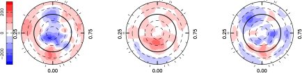
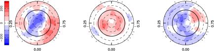
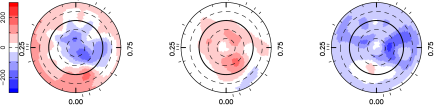
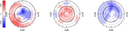
Figure 3: ZDI maps of the radial (left), meridional (middle) and azimuthal (right) magnetic field components for the 8 subsets associated with the following epochs: 2020 Aug-Sep, 2020 Sep-Oct 2020, 2020 Dec - 2021 Jan, 2021 Oct, 2021 Nov-Dec, 2022 Jan, 2022 Nov and 2023 Jan. The star is shown in a flattened polar view down to $-60^{\circ}$, with the pole at the center, the equator depicted as a bold circle and the black$-30^{\circ}$, 30^∘ and $60^{\circ}$ latitude parallels represented by dashed circles. Positive radial, meridional and azimuthal fields are shown in red and point outwards, polewards and counter-clockwise, respectively. The ticks around the star refer to the phases of the SPIRou spectropolarimetric observations used in ZDI. These maps were obtained blackassuming the mean differential rotation derived in Sec. 3.3 and are shown at mid-time throughout the corresponding subset.

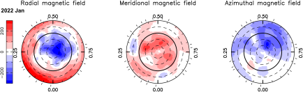
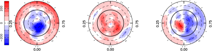
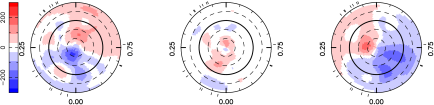
Figure 4: Continued.

Despite a rapid evolution of the longitudinal field, we find that the magnetic topology of this star remains mainly poloidal, this component enclosing between black65% (2021 Oct) and black90% (2020 Aug-Sep) of the reconstructed magnetic energy, more than black45% of which being concentrated in axisymmetric modes, until 2023 Jan (see Table 3). This field component mainly consists of a dipole, whose inclination with respect to the rotation axis is low ($<35^{\circ}$) until 2023 Jan and whose strength ranges from black85 to 245 G. In 2023 Jan, we see a change in the topology, especially for the radial component of the field, with the dipole component of the poloidal field being now tilted at black75^∘, potentially suggesting the beginning of a polarity reversal. To investigate this point further and find out whether this evolution is real or rather caused by, e.g., limited data sampling, we carried out the following experiment. Using the ZDI map of 2022 Nov, we simulated a dataset with the same phase coverage and SNR as that of our 2023 Jan data, and applied ZDI to these simulated data. As the reconstructed large-scale magnetic topology is close to the input field, we can conclude that the strong tilt of the magnetic topology that we report from out 2023 Jan data is likely real.

The large-scale magnetic topology of V1298 Tau also features a significant toroidal field, enclosing between black10% (2020 Aug-Sep) and black35% (2021 Oct) of the reconstructed magnetic energy, and found to be mainly axisymmetric and dipolar. We also find that the quadratically-averaged large-scale magnetic flux over the stellar surface, noted <$B_{V}$>, blackvaries by $\mathord{\sim}80$% between 2020 Aug and 2022 Nov (from 100 to 180 G).

Table 3: Properties of the large-scale magnetic field of V1298 Tau between 2020 and 2023, from ZDI reconstruction black(including differential rotation) of 8 datasets. Columns 1–2 show the number of the dataset and the associated epoch. Columns 3 to 5 list the quadratically-averaged large-scale magnetic flux over the stellar surface, the strength and tilt, with respect to the stellar rotation axis, of the dipole (of the poloidal component). The two last columns gather the fraction of reconstructed magnetic energy enclosed by the poloidal/toroidal components of the field and in the axisymmetric modes of these components. The typical error bars on these values are of 5-10%.

Dataset	Epoch	<$B_{V}$>	$B_{d}$	Tilt	Poloidal	Toroidal
		(G)	(G)	(∘)	(%)
#1	2019 Oct	70	30	80	85 / 5	15 / 20
#2	2019 Nov-Dec	40	15	25	90 / 10	10 / 15
#3	2020 Aug-Sep	120	145	30	90 / 50	10 / 15
#4	2020 Sep-Oct	100	90	15	80 / 45	20 / 55
#5	2020 Dec - 2021 Jan	125	130	30	85 / 55	15 / 70
#6	2021 Oct	125	125	25	65 / 65	35 / 85
#7	2021 Nov-Dec	120	145	35	75 / 60	25 / 90
#8	2022 Jan	180	245	30	85 / 70	20 / 75
#9	2022 Nov	165	210	15	90 / 65	10 / 70
#10	2023 Jan	100	85	75	80 / 10	20 / 55

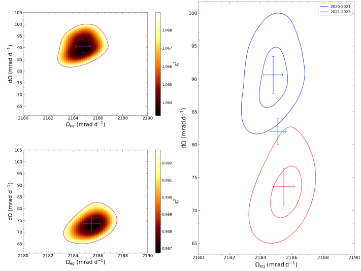
Figure 5: Surface differential rotation of V1298 Tau as measured from SPIRou data blackduring the 2020 Aug - 2021 Jan (upper left) and 2021 Sep - 2022 Feb (bottom left) seasons. $\chi^{2}_{r}$ maps computed from Stokes $V$ LSD profiles over a grid of parameters $\Omega_{\rm eq}$, the rotation rate at the equator, and d$\Omega$ the difference in rotation rate between the pole and the equator. Red blackcontours show the $3\sigma$ confidence blackinterval, while the magenta crosses depict the optimal value with its associated error bars, derived from the fit of a 2D paraboloid close to the minimum of the grid. The right panel shows the contours associated with $1\sigma$ and $3\sigma$ confidence blackintervals obtained from both observing seasons (black2020 Aug - 2021 Jan: blue; 2021 Sep - 2022 Feb: red). The magenta cross depicts the mean parameters.

3.3 Differential rotation

From ZDI reconstructions, we see that our data show some variability within each observing season. Part of this variability can potentially be due to surface differential rotation. One can use ZDI to estimate DR by assuming that the surface shear follows a solar-like law given by:

$$\Omega(\theta)=\Omega_{\rm eq}-\left(\cos{\theta}\right)^{2}\,\mathrm{d}\Omega$$ (4)

where $\Omega_{\rm eq}$ and d$\Omega$ correspond to the parameters of the DR law, i.e. the rotation rate at the equator and the pole-to-equator rotation rate difference, respectively, and $\theta$ represents the colatitude.

As our subsets cover up to $\mathord{\sim}40$ d, we need to merge some of them to diagnose subtle temporal variations of the Stokes $V$ LSD profiles under the effect of DR. We thus estimated DR during the 2020 Aug - 2021 Jan season from subsets #3 to #5 (black49 Stokes $V$ profiles spanning 135 d, i.e. $\mathord{\sim}46$ rotation cycles), and during the 2021 Sep - 2022 Feb season from subsets #6 to #8 (black47 observations spanning 109 d, i.e. $\mathord{\sim}37$ rotation cycles). The Zeeman signatures collected between 2019 Oct and Dec are blackboth too noisy and too sparse to provide us with reliable estimates of DR, while mediocre phase coverage in 2023 and the sudden evolution of the overall topology between the first half and the second half of the 2022 Nov - 2023 Feb season prevents us to blackestimate DR at blackthis time.

In practice, we fitted these blacktwo subsets of Stokes $V$ LSD profiles at a given amount of information (i.e. magnetic energy), over a grid of DR parameters. This process yielded $\chi^{2}_{r}$ maps from which we estimated the optimal values for both $\Omega_{\rm eq}$ and d$\Omega$ and their associated error bars by adjusting a 2D paraboloid close to the minimum (Donati et al., 2000; Petit et al., 2002; Donati et al., 2003b; Finociety et al., 2021, 2023).

blackFrom Stokes $V$ LSD profiles collected during the 2020 Aug - 2021 Jan season (subsets #3 to #5), we find $\Omega_{\rm eq}=2184.8\pm 0.6$ $\rm mrad\,d^{-1}$ and d$\Omega=90.6\pm 2.8$ $\rm mrad\,d^{-1}$. This implies that the rotation period ranges from $2.876\pm 0.001$ d at the equator to $3.000\pm 0.004$ d at the pole. For the 2021 Sep - 2022 Feb season (subsets #6 to #8), we find a weaker level of DR with $\Omega_{\rm eq}=2185.5\pm 0.7$ $\rm mrad\,d^{-1}$ and d$\Omega=73.5\pm 2.8$ $\rm mrad\,d^{-1}$, corresponding to a period at the equator and at the pole of $2.875\pm 0.001$ and $2.975\pm 0.004$ d, respectively.

While both estimates of $\Omega_{\rm eq}$ are consistent, estimates of d$\Omega$ differ blackby more than $3\sigma$, suggesting that the DR may vary at the surface of V1298 Tau between the two consecutive observing seasons (see Fig. 5). In addition, for both observing seasons, the confidence blackcontours are slightly distorted, reflecting that the $\chi^{2}_{r}$ maps are not perfect 2D paraboloids, especially when blackmoving away from the minimum of the maps, which likely increases the size of the error bars.

The higher level of DR measured from black2020 Aug - 2021 Jan data is consistent with the evolution of the longitudinal field. blackWe indeed estimate a lower decay time-scale of $B_{\ell}$ during this observing season, indicating a faster evolution of the blacklarge-scale field that may partly reflect a stronger DR.

We chose a unique set of parameters to describe the DR at the surface of V1298 Tau, computed as the weighted means of the estimates provided by both considered observing seasons, blacki.e. $\Omega_{\rm eq}=2185.1\pm 0.5$ $\rm mrad\,d^{-1}$ and d$\Omega=82.0\pm 2.0$ $\rm mrad\,d^{-1}$. These values imply that the equator of the star rotates with a period of $2.875\pm 0.001$ d while the pole rotates in $2.988\pm 0.003$ d, the equator lapping the pole by one cycle in $\mathord{\sim}76$ d, i.e. about half an observing season. Using these values, we find that both our $B_{\ell}$ (Sec. 3.1) and RV data (Sec. 4.2), with a period of $2.910\pm 0.005$ and $2.909\pm 0.009$ d, respectively, probe the same latitudes of about 30^∘ (between 31–37^∘ and 28–39^∘, respectively).

Splitting each data sets in two subsets, each covering about half the observing season, and carrying the same analysis yield discrepant DR parameters, with error bars up to 3 times larger than blackthose mentioned above, demonstrating that a large number of Stokes $V$ profiles collected over the whole observing season are needed to reliably estimate the DR parameters.

3.4 Time-dependent Imaging of Magnetic Stars

As our data are spread over several years, we also applied the new blacktomographic method named Time-dependent Imaging of Magnetic Stars (TIMeS) blackoutlined in Finociety & Donati (2022). As for ZDI, this method aims at finding the simplest large-scale magnetic topology consistent with the data (i.e. Stokes $V$ LSD profiles) but this time allowing it to evolve with time. TIMeS uses sparse approximations to identify as few spherical harmonic modes (associated with $\alpha_{\ell,m}$, $\beta_{\ell,m}$ and $\gamma_{\ell,m}$ coefficients) as possible to reconstruct the magnetic topology and GPs to model the time-dependence of each identified coefficients. This method can only be applied in the cases where the magnetic field is not too strong, typically with a magnetic flux lower than $\mathord{\sim}3$ kG for a $v\sin{i}=25$ $\mathrm{km}\,\mathrm{s}^{-1}$. Given the $v\sin{i}$ of V1298 Tau and the values of <$B_{V}$> blackand of the local field inferred from the ZDI reconstructions in the previous sections ($\ll 3$ kG), we therefore assume that TIMeS can be applied to our data.

In practice, thanks to the principle of sparsity, we first look for the simplest linear combination of known magnetic topologies that blackprovides a satisfactory fit to subsets of $n$ consecutive profiles, assuming that the blacklarge-scale magnetic field does not significantly evolve over the time span covered by the $n$ profiles. We did not blackconsider the subsets for which 2 consecutive profiles are separated by more than twice the decay time-scale of the longitudinal field. As mentioned in Finociety & Donati (2022), the $n$ profiles should sample the rotation cycle while blacktypically covering 10 to 20% of the decay time-scale of the longitudinal field, explaining why we set $n=6$ in this paper (corresponding to $\mathord{\sim}20$% of the $B_{\ell}$ decay time-scale). This first step yields the spherical harmonic modes that significantly contribute to the overall topology over the whole dataset, with a value of the corresponding $\alpha_{\ell,m}$, $\beta_{\ell,m}$ and $\gamma_{\ell,m}$ coefficients for each subset. TIMeS then models these time series of coefficients using GPs with a squared exponential kernel, allowing one to compute the magnetic maps and associated Stokes $V$ LSD profiles for each observed rotation cycle.

blackWe applied TIMeS to all the Stokes $V$ LSD profiles covering black2020 Aug - 2023 Feb (i.e. subsets #3 to #10) at once, blackallowing all spherical harmonic modes up to $\ell_{\rm max}=10$ (as in ZDI, see Sec. 3.2) and assuming $i=70^{\circ}$ to better identify axisymmetric structures (e.g. dipole) that are missed when using $i=80^{\circ}$. We were able to fit the data down to $\chi^{2}_{r}=1.49$, revealing that the model does not succeed in fitting the data down to the noise level, likely due to the limited available resolution at the surface of the star, the model only featuring 11 modes up to $\ell=4$, even though $\ell_{\max}=10$. We show the reconstructed magnetic maps during the black2020 Aug - 2021 Jan season at specific rotation cycles in Figs. 6, 7 and 8 while those associated with black2021 Sep - 2022 Feb and 2022 Nov - 2023 Feb data can be seen in Appendix C (Figs. 20 to 24). The synthetic Stokes $V$ LSD profiles obtained with TIMeS are also shown in Fig. 25. Despite some loss of blackspatial resolution, we find that the reconstructed maps are blackquite similar to those obtained with ZDI at the same epochs, with only a subtle evolution within each subset considered in the previous sections (as expected from the unit $\chi^{2}_{r}$ obtained with ZDI). In particular, we identify the same topology for the radial field and the blacksimilar large blackfeatures in the azimuthal field (e.g. around phases 0.35-0.45 in blacklate 2020).

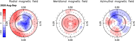
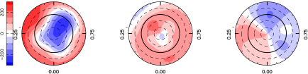
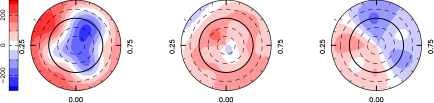
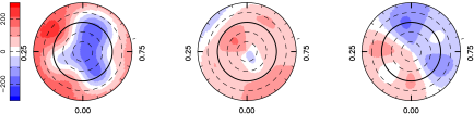
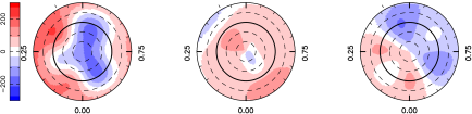
Figure 6: Magnetic maps in 2020 Aug-Sep reconstructed with ZDI without differential rotation (first row) and TIMeS (second blackto fifth rows). As TIMeS allows the reconstruction of a map at each observed date, we only show blackfour specific epochs indicated on the left. See Fig. 3 for a detailed description of the Figure.

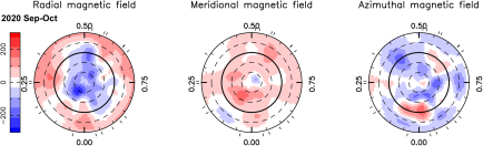
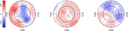
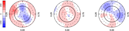
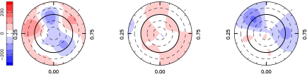
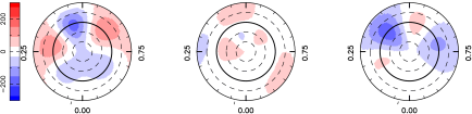
Figure 7: Same as Fig. 6 for 2020 Sep-Oct.

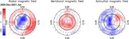
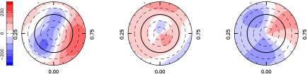
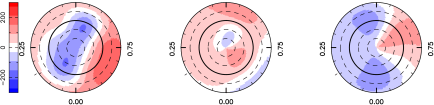
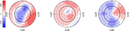
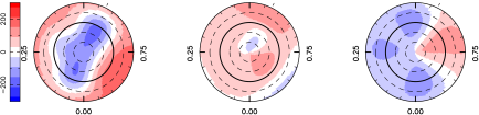
Figure 8: Same as Fig. 6 for 2020 Dec - 2021 Jan.

blackThis first application of TIMeS blackto real data therefore demonstrates that this method is efficient at reconstructing reliable magnetic topologies even if the data blackspan several years, with only a small amount of information that is not reconstructed (especially the smallest features). In addition, we find that the fraction of the magnetic energy enclosed in the poloidal field is globally consistent with that derived from ZDI applied on each subset, except for subsets #6 and #10 which likely results from the loss of blackspatial resolution with TIMeS (Fig. 9).

Using Lomb-Scargle periodograms (Zechmeister & Kürster, 2009) with the astropy python module on each of the $\alpha_{\ell,m}$, $\beta_{\ell,m}$ and $\gamma_{\ell,m}$ coefficients found with TIMeS does not reveal any common periodicity (see Fig. 26), suggesting that we blackdid not yet detect a magnetic cycle in our data, which is not surprising given that only a hint of a first polarity switch has been observed up to now. Future observations of V1298 Tau will blackallow us to conclude whether the putative change in the poloidal field polarity is confirmed, and is part of a cycle much longer than the time span of our current observations.

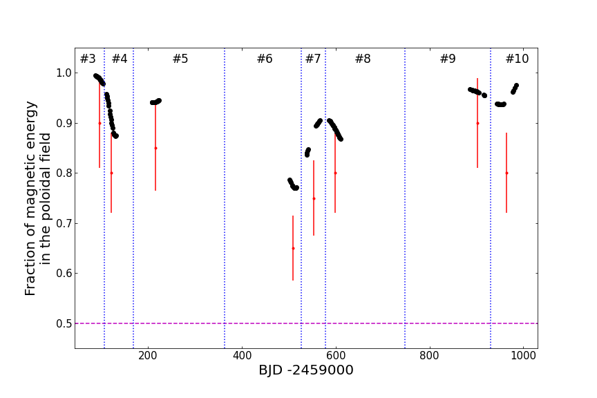
Figure 9: Evolution with time of the poloidal component of the field between 2020 and 2023. In black, we show the fraction of the reconstructed magnetic energy enclosed in the poloidal field, estimated using TIMeS. The red points correspond to the value reconstructed from ZDI applied on each subsets, blackassuming typical error bars of 10% (see Table 3). The vertical blue dotted lines depict the limits between each subsets used in ZDI (with their number at the top of the plot) while the magenta dashed line denotes the limit above which the magnetic field is mainly poloidal (i.e. more than 50% of the reconstructed magnetic energy is enclosed in the poloidal component).

4 Characterizing the multi-planet system

4.1 Orbital period of planet e

We analysed the RVs obtained from the data reduction performed with APERO using the LBL method (Artigau et al., 2022) in order to look for the RV signatures induced by the 4 transiting planets hosted by V1298 Tau. The orbital period and transit times of these planets were accurately determined by Feinstein et al. (2022), except for planet e for which the orbital period is still unknown (but longer than 40 d; Suárez Mascareño et al. 2021; Feinstein et al. 2022; Sikora et al. 2023). Using these values (see Table 4) and assuming circular orbits for all planets (consistent with the results of Suárez Mascareño et al. 2021 and Sikora et al. 2023), we only need to retrieve the semi-amplitude of the planet RV signatures ($K_{b}$, $K_{c}$, $K_{d}$ and $K_{e}$ for planet b, c, d and e, respectively) as well as the orbital period of planet e, noted $P_{e}$, from our data.

In practice, we used a model featuring a QP GP to model the RV signal induced by stellar activity, 4 Keplerian curves associated with the planet signatures (assuming circular orbits) and an additional white noise (e.g. due to intrinsic variability). As for the longitudinal field, we sampled the posterior distribution of each parameter (planet and GP) using a MCMC method to estimate their optimal value.

We note that the posterior distribution of $P_{e}$ is multimodal if we impose a uniform prior on the orbital period of planet e (between 42 and 65 d, following the list of probable periods of Feinstein et al. 2022), showing 1 global maximum at about 53.5 d and three local maxima at 42.7 d, 46.4 d and 60.6 d (see Fig. 27). We therefore run our process again, each time with a narrow Gaussian prior centred on one of these periods with a standard deviation of 1 d to investigate which one is the most likely. We then computed the marginal logarithmic likelihood $\log\mathcal{L_{M}}$ following the method described by Chib & Jeliazkov (2001), in order to estimate the significance of one solution with respect to the others from the difference in $\log\mathcal{L_{M}}$ (i.e. logarithmic Bayes Factor / log BF). Considering the model featuring an orbital period for planet e at $53.5$ d as the reference, we find that the log BF for the 3 other models (associated with an orbital period of $42.7$, $46.4$ and $60.6$ d, respectively) is equal to $-1.4$, $-2.4$ and $-4.1$, suggesting that the model featuring a prior centred on an orbital period of $53.5$ d is more likely than the three others. From the MCMC approach, we therefore estimate the most likely orbital period to be $P_{e}=53.5\pm 0.4$ d and we thus use this model to further characterize the 4 planets in the following.

4.2 Planet masses

With our reference model, we are able to fit our data down to $\chi^{2}_{r}=5.97$ with the residuals exhibiting a RMS dispersion of 34.8 $\mathrm{m}\,\mathrm{s}^{-1}$. This value for the $\chi^{2}_{r}$ suggest that discrepancies exist between the model and our measurements and that our error bars (estimated from photon noise) are likely underestimated, e.g. due to intrinsic variability that has not be taken into account. More generally, our detections of the planet-induced RV variations are limited by the high level of stellar activity compared to the recovered planet RV signatures (GP amplitude of $\mathord{\sim}120$ $\mathrm{m}\,\mathrm{s}^{-1}$, i.e. 2.6 to 28 times larger than the semi-amplitude of the planet signatures) and of intrinsic variability (modeled by the additional white noise, equal to $46\pm 5$ $\mathrm{m}\,\mathrm{s}^{-1}$, i.e. $3\times$ larger than the typical error bar of 14 $\mathrm{m}\,\mathrm{s}^{-1}$) of V1298 Tau. In particular, we find that the decay time-scale is equal to $32^{+6}_{-5}$ d, compatible with the one derived from $B_{\ell}$ measurements, indicating that the surface of the star evolves rapidly. The GP is also modulated by the stellar rotation with a period equal to $2.909\pm 0.009$ d, blacksimilar to the one found from $B_{\ell}$ measurements. All these results clearly illustrate the need for robust filtering methods given how difficult the detection of planets around young active stars is, even when their ephemerides (orbital periods, transit times) are well determined.

Despite this intense activity, we find that planet e is best detected, at a $3.9\sigma$ level, with a RV semi-amplitude $K_{e}=47^{+16}_{-12}$ $\mathrm{m}\,\mathrm{s}^{-1}$, associated with a mass $M_{e}=1.01^{+0.35}_{-0.26}$ M_♃ (for an orbital period of $53.5\pm 0.4$ d). Assuming a radius of $0.89\pm 0.04$ R_♃, following Feinstein et al. (2022), the planet density is found to be $\rho_{e}=1.79^{+0.66}_{-0.51}$ $\rm g\,cm^{-3}$.

For the three innermost planets, we do not obtain clear detections as we find $K_{b}=4.2\pm 10.7$ $\mathrm{m}\,\mathrm{s}^{-1}$, $K_{c}=4.8\pm 6.2$ $\mathrm{m}\,\mathrm{s}^{-1}$ and $K_{d}=4.9\pm 6.7$ $\mathrm{m}\,\mathrm{s}^{-1}$, corresponding to masses of $M_{b}=0.07\pm 0.18$ M_♃, $M_{c}=0.05\pm 0.07$ M_♃ and $M_{d}=0.05\pm 0.08$ M_♃, and densities of $\rho_{b}=0.14\pm 0.36$ $\rm g\,cm^{-3}$, $\rho_{c}=0.76\pm 0.99$ $\rm g\,cm^{-3}$ and $\rho_{d}=0.40\pm 0.66$, respectively. Based on the 99% confidence level interval associated with the posterior distribution of each planet mass blackderived with the MCMC approach (after converting the sampled semi-amplitudes into masses), we derive upper limits on these masses of $M_{b}<0.44$ M_♃, $M_{c}<0.22$ M_♃ and $M_{d}<0.25$ M_♃. We summarize all the planet parameters in Table 4 for the 4 best periods and we show the associated corner plots in Appendix D. We also show the best fit (i.e. for $P_{e}=53.5$ d) and the associated phase-folded filtered RVs in Figs. 10 and 11, respectively.

Assuming an eccentric orbit for planet e (in the case of the most likely orbital period of 53.5 d), yields no improvement in confidence level ($\log{\rm BF}=-0.7$ with respect to our best model) and an eccentricity consistent with 0 ($0.03\pm 0.05$), indicating a posteriori that our previous assumption of circular orbits was justified to model our data.

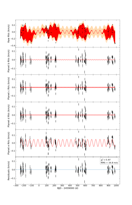
Figure 10: RVs of V1298 Tau between end 2019 and early 2023. The first panel shows the raw RVs (black dots) along with the best model (including the activity jitter and the planet sginatures) in red and the $1\sigma$ confidence level in light orange. 2^nd to 5^th panels show the retrieved RV signatures of planets b, c, d and e, respectively. The last panel shows the residuals RVs, having a RMS dispersion of 24.3 $\mathrm{m}\,\mathrm{s}^{-1}$, i.e. close to the typical error bar of our measurements.

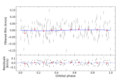
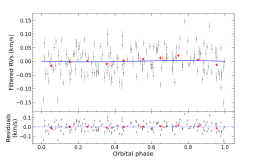
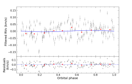
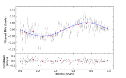
Figure 11: Phase-folded filtered (top panels) and residuals (bottom panels) RVs for planets b (1^st panel), c (2^nd panel), d (3^rd panel) and e (4^th panel). The 174 measured RVs are shown as black dots (with their error bar) while the red stars correspond to RVs averaged over 0.1 orbital cycle. The RV signature (derived from our MCMC process) associated with each planet is shown as a blue solid line. The RMS dispersion of the residuals is equal to 34.8 $\mathrm{m}\,\mathrm{s}^{-1}$ (see Fig. 10).

In addition, we computed the Lomb-Scargle periodograms of the raw RVs, filtered RVs and residuals RVs to look for potential additional planets that may have not been detected before (e.g. non-transiting planets). blackLooking at the raw RVs, we do not see any significant peak at 1 yr (with a FAP lower than 10%), suggesting that the contamination of our data from telluric lines is insignificant for our purpose. When focussing on the filtered RVs (in which only activity was removed), we see a significant power at the orbital period of planet e, but no clear peak in the periodogram of the residual RVs (see Fig. 12). blackWe simulated RV datasets with the same temporal distribution as our actual SPIRou data using our best model on which we added the signature of a potential fifth planet beyond the orbit of V1298 Tau e. Using these datasets, we estimate that only planets more massive than $2.7$ and 5.9 M_♃ at 0.7 and 1.4 au (corresponding to an orbital period of 6 months and $1.5$ yr), respectively, could be reliably detected with our dataset.

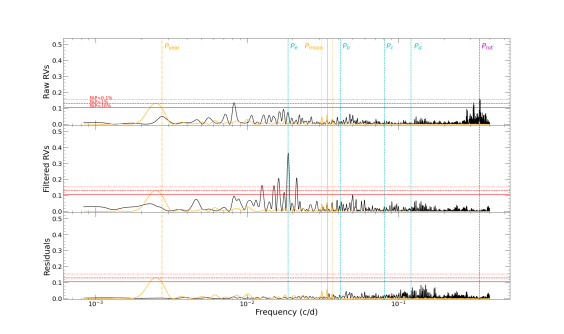
Figure 12: Lomb-Scargle periodograms of the raw RVs (top), filtered RVs (middle) and residuals (bottom) computed using the astropy python module. The horizontal dotted, dashed and solid red lines depict the FAPs of 0.1, 1 and 10%, respectively. The vertical dashed magenta line corresponds to the stellar rotation period while the dashed cyan lines show the orbital periods of planets e, b, c and d (from left to right). blackThe orange curve depicts the window function, the orange solid and dotted vertical lines correspond to the synodic period of the Moon and its 1-yr aliases, respectively, and the orange dashed vertical line outlines the 1-yr period.

Table 4: MCMC results for the analysis of the RV data. 1^st and 2^nd columns list the parameters and their associated priors corresponding to a model featuring an activity signal and four planet-related RV signatures. The 4 last columns show the best value for each parameter, in the case of a narrow prior centred on 3 different values of $P_{e_{0}}$ for the orbital period of planet e. blackThe knee of the modified Jeffreys priors is set to the typical RV uncertainty, noted $\sigma_{RV}$. Note that the $\log{\rm BF}$ is computed with respect to the marginal likelihood associated with $P_{e_{0}}=53.5$ d.

Parameter	Prior	$P_{e_{0}}=53.5$ d	black$P_{e_{0}}=42.7$ d	black$P_{e_{0}}=46.4$ d	$P_{e_{0}}=60.6$ d
$\theta_{1}$ ($\mathrm{km}\,\mathrm{s}^{-1}$)	mod Jeffreys ($\sigma_{RV}$)	$0.12\pm 0.01$	$0.13\pm 0.01$	$0.13\pm 0.01$	$0.12\pm 0.01$
$\theta_{2}$ (d)	log Gaussian ($\log 30$, $\log 2$)	black$32^{+6}_{-5}$	black$28^{+5}_{-4}$	black$31^{+5}_{-4}$	black$30^{+6}_{-5}$
$\theta_{3}$ (d)	Gaussian (2.91, 0.1)	black$2.909\pm 0.009$	black$2.921\pm 0.010$	black$2.904\pm 0.010$	black$2.923\pm 0.008$
$\theta_{4}$	Uniform (0, 3)	black$0.28\pm 0.05$	black$0.28\pm 0.06$	black$0.32\pm 0.06$	black$0.24\pm 0.05$
$\theta_{5}$ ($\mathrm{m}\,\mathrm{s}^{-1}$)	mod Jeffreys ($\sigma_{RV}$)	black$46\pm 5$	black$45^{+5}_{-4}$	black$46\pm 5$	black$46\pm 5$
$K_{b}$ ($\mathrm{m}\,\mathrm{s}^{-1}$)	mod Jeffreys ($\sigma_{RV}$)	black$4.2\pm 10.7$	black$6.3\pm 10.6$	black$5.1\pm 11.6$	black$3.3\pm 10.9$
$P_{b}$ (d)	Fixed from Feinstein et al. (2022)	24.1315	24.1315	24.1315	24.1315
$T_{b}$ (2459000+)	Fixed from Feinstein et al. (2022)	481.0902	481.0902	481.0902	481.0902
$R_{b}$ (R♃)	Fixed from Feinstein et al. (2022)	0.85	0.85	0.85	0.85
$M_{b}$ (M♃)	Derived from $K_{b}$, $P_{b}$ and $M_{*}$	black$0.07\pm 0.18$	black$0.11\pm 0.18$	black$0.08\pm 0.19$	black$0.05\pm 0.18$
$\rho_{b}$ ($\rm g\,cm^{-3}$)	Derived from $M_{b}$ and $R_{b}$	black$0.14\pm 0.36$	black$0.21\pm 0.36$	black$0.17\pm 0.39$	black$0.11\pm 0.37$
$K_{c}$ ($\mathrm{m}\,\mathrm{s}^{-1}$)	mod Jeffreys ($\sigma_{RV}$)	black$4.8\pm 6.2$	black$3.8\pm 6.3$	black$5.5\pm 6.3$	black$3.8\pm 6.3$
$P_{c}$ (d)	Fixed from Feinstein et al. (2022)	8.2438	8.2438	8.2438	8.2438
$T_{c}$ (2459000+)	Fixed from Feinstein et al. (2022)	481.1664	481.1664	481.1664	481.1664
$R_{c}$ (R♃)	Fixed from Feinstein et al. (2022)	0.45	0.45	0.45	0.45
$M_{c}$ (M♃)	Derived from $K_{c}$, $P_{c}$ and $M_{*}$	black$0.05\pm 0.07$	black$0.04\pm 0.07$	black$0.06\pm 0.07$	black$0.04\pm 0.07$
$\rho_{c}$ ($\rm g\,cm^{-3}$)	Derived from $M_{c}$ and $R_{c}$	black$0.76\pm 0.99$	black$0.60\pm 1.00$	black$0.86\pm 1.00$	black$0.61\pm 1.00$
$K_{d}$ ($\mathrm{m}\,\mathrm{s}^{-1}$)	mod Jeffreys ($\sigma_{RV}$)	black$4.9\pm 6.7$	black$4.4\pm 6.5$	black$6.0\pm 6.6$	black$5.8\pm 7.0$
$P_{d}$ (d)	Fixed from Feinstein et al. (2022)	12.3960	12.3960	12.3960	12.3960
$T_{d}$ (2459000+)	Fixed from Feinstein et al. (2022)	478.4149	478.4149	478.4149	478.4149
$R_{d}$ (R♃)	Fixed from Feinstein et al. (2022)	0.55	0.55	0.55	0.55
$M_{d}$ (M♃)	Derived from $K_{d}$, $P_{d}$ and $M_{*}$	black$0.05\pm 0.08$	black$0.06\pm 0.08$	black$0.08\pm 0.08$	black$0.07\pm 0.09$
$\rho_{d}$ ($\rm g\,cm^{-3}$)	Derived from $M_{d}$ and $R_{d}$	black$0.40\pm 0.66$	black$0.43\pm 0.65$	black$0.60\pm 0.66$	black$0.58\pm 0.70$
$K_{e}$ ($\mathrm{m}\,\mathrm{s}^{-1}$)	mod Jeffreys ($\sigma_{RV}$)	black$47^{+16}_{-12}$	black$44^{+21}_{-14}$	black$36^{+18}_{-12}$	black$25^{+24}_{-12}$
$P_{e}$ (d)	Gaussian ($P_{e_{0}}$, 1)	black$53.5\pm 0.4$	black$42.7\pm 0.3$	black$46.4\pm 0.4$	black$60.6\pm 0.7$
$T_{e}$ (2459000+)	Fixed from Feinstein et al. (2022)	481.7967	481.7967	481.7967	481.7967
$R_{e}$ (R♃)	Fixed from Feinstein et al. (2022)	0.89	0.89	0.89	0.89
$M_{e}$ (M♃)	Derived from $K_{e}$, $P_{e}$ and $M_{*}$	black$1.01^{+0.35}_{-0.26}$	black$0.87^{+0.41}_{-0.28}$	black$0.75^{+0.37}_{-0.25}$	black$0.56^{+0.54}_{-0.27}$
$\rho_{e}$ ($\rm g\,cm^{-3}$)	Derived from $M_{e}$ and $R_{e}$	black$1.79^{+0.66}_{-0.51}$	black$1.53^{+0.76}_{-0.54}$	black$1.31^{+0.67}_{-0.47}$	black$0.99^{+0.96}_{-0.50}$
$\chi^{2}_{r}$		black5.97	black5.53	black5.92	black5.74
RMS ($\mathrm{m}\,\mathrm{s}^{-1}$)		black34.8	black33.8	black34.8	black34.4
$\log\mathcal{L_{M}}$		black$-215.5$	black$-216.9$	${\color{black}{{-217.9}}}$	black$-219.6$
log BF		0	black$-1.4$	black$-2.4$	black$-4.1$

4.3 Additional constraints from previous studies

From the transit times of planet e in the TESS and K2 light curves, Feinstein et al. (2022) derived 17 probable orbital periods for this planet. We therefore modeled our data, blackassuming circular orbits, this time imposing a Gaussian prior on the orbital period of this planet centered on each of these values with a standard deviation of 0.0001, corresponding to the typical error bar reported by Feinstein et al. (2022).

From the $\log\mathcal{L_{M}}$, we find that the most likely period is $P_{e}=53.0039\pm 0.0001$ d, blackyielding a fit to our RV data associated with a $\chi^{2}_{r}=6.30$ and a RMS dispersion of the residuals of 35.8 $\mathrm{m}\,\mathrm{s}^{-1}$. For this period, we report a 4$\sigma$ detection of the RV signature of planet e ($K_{e}=44^{+15}_{-11}$ $\mathrm{m}\,\mathrm{s}^{-1}$) associated with a mass of $M_{e}=0.95^{+0.33}_{-0.24}$, while the 3 other planets remain undetected.

Using this value as a reference, we computed the log BF between this model and the 16 others. From this criterion, we cannot blackdefinitely rule out any of the 17 periods provided by Feinstein et al. (2022) as all periods yield a $|\log{\rm BF}|<6.4$. We however distinguish 3 groups: the most likely periods ($|\log{\rm BF}|<2.5$), the plausible periods ($2.5<|\log{\rm BF}|<5$) and the blackleast likely periods ($|\log{\rm BF}|\geq 5$). In addition to $P_{e}=53.0039$ d, 3 other values belong to the most likely group ($P_{e}=54.2085$, 46.7681 and 45.8687 d, associated with log BF of $-1.1$, $-2.0$ and $-2.4$ respectively). The intermediate plausible group contains 6 orbital periods ($P_{e}=45.0033$, 47.7035, 48.6770, 59.6294, 61.1583 and 62.7678 d), that are still considered as potential values, even though the derived mass for planet e can be more than twice smaller than that obtained in Sec. 4.2 or in the most likely group. The least likely group therefore gathers the 7 remaining values ($P_{e}=44,1699$, 49.6911, 50.7484, 51.8516, 55.4692, 56.7899 and 58.1750 d). We summarized the results for the 4 most likely orbital periods in Table 5, while those associated with the plausible and least likely groups are given in Tables 10 and 11, respectively.

As for the previous case in Sec. 4.2, estimating the eccentricity of planet e as part of the process does not signifcantly improve the results (e.g. $\log{\rm BF}=0.2$).

Table 5: MCMC results for the analysis of the RV data for the 4 most likely planet e orbital periods derived by Feinstein et al. (2022). 1^st and 2^nd columns list the parameters and their associated priors corresponding to a model featuring an activity signal and four planet-related RV signatures. The 4 last columns show the best value for each parameter, in the case of a narrow prior centred on different values of $P_{e_{0}}$ for the orbital period of planet e. blackThe knee of the modified Jeffreys priors is set to the typical RV uncertainty, noted $\sigma_{RV}$. Note that the $\log{\rm BF}$ is computed with respect to the marginal logarithmic likelihood associated with $P_{e_{0}}=53.0039$ d.

Parameter	Prior	$P_{e_{0}}=53.0039$ d	$P_{e_{0}}=54.2085$ d	$P_{e_{0}}=46.7681$ d	$P_{e_{0}}=45.8687$ d
$\theta_{1}$ ($\mathrm{km}\,\mathrm{s}^{-1}$)	mod Jeffreys ($\sigma_{RV}$)	$0.13\pm 0.01$	$0.12\pm 0.01$	$0.13\pm 0.01$	$0.13\pm 0.01$
$\theta_{2}$ (d)	log Gaussian ($\log 30$, $\log 2$)	black$33^{+6}_{-5}$	black$30^{+6}_{-5}$	black$32^{+5}_{-4}$	black$29^{+5}_{-4}$
$\theta_{3}$ (d)	Gaussian (2.91, 0.1)	black$2.907\pm 0.009$	black$2.917\pm 0.009$	black$2.906\pm 0.008$	black$2.906\pm 0.012$
$\theta_{4}$	Uniform (0, 3)	black$0.30\pm 0.06$	black$0.25\pm 0.05$	black$0.31\pm 0.06$	black$0.32\pm 0.06$
$\theta_{5}$ ($\mathrm{m}\,\mathrm{s}^{-1}$)	mod Jeffreys ($\sigma_{RV}$)	black$47\pm 5$	black$45\pm 5$	black$45\pm 5$	black$47\pm 5$
$K_{b}$ ($\mathrm{m}\,\mathrm{s}^{-1}$)	mod Jeffreys ($\sigma_{RV}$)	black$4.1\pm 10.8$	black$3.5\pm 11.0$	black$6.1\pm 11.6$	black$3.7\pm 11.5$
$P_{b}$ (d)	Fixed from Feinstein et al. (2022)	24.1315	24.1315	24.1315	24.1315
$T_{b}$ (2459000+)	Fixed from Feinstein et al. (2022)	481.0902	481.0902	481.0902	481.0902
$R_{b}$ (R♃)	Fixed from Feinstein et al. (2022)	0.85	0.85	0.85	0.85
$M_{b}$ (M♃)	Derived from $K_{b}$, $P_{b}$ and $M_{*}$	black$0.07\pm 0.18$	black$0.06\pm 0.18$	black$0.11\pm 0.19$	black$0.06\pm 0.19$
$\rho_{b}$ ($\rm g\,cm^{-3}$)	Derived from $M_{b}$ and $R_{b}$	black$0.14\pm 0.36$	black$0.12\pm 0.37$	black$0.20\pm 0.39$	black$0.13\pm 0.39$
$K_{c}$ ($\mathrm{m}\,\mathrm{s}^{-1}$)	mod Jeffreys ($\sigma_{RV}$)	black$5.7\pm 6.5$	black$4.1\pm 6.2$	black$5.7\pm 6.3$	black$4.9\pm 6.1$
$P_{c}$ (d)	Fixed from Feinstein et al. (2022)	8.2438	8.2438	8.2438	8.2438
$T_{c}$ (2459000+)	Fixed from Feinstein et al. (2022)	481.1664	481.1664	481.1664	481.1664
$R_{c}$ (R♃)	Fixed from Feinstein et al. (2022)	0.45	0.45	0.45	0.45
$M_{c}$ (M♃)	Derived from $K_{c}$, $P_{c}$ and $M_{*}$	black$0.06\pm 0.07$	black$0.04\pm 0.07$	black$0.06\pm 0.07$	black$0.05\pm 0.07$
$\rho_{c}$ ($\rm g\,cm^{-3}$)	Derived from $M_{c}$ and $R_{c}$	black$0.90\pm 1.03$	black$0.64\pm 0.98$	black$0.89\pm 1.00$	black$0.78\pm 0.97$
$K_{d}$ ($\mathrm{m}\,\mathrm{s}^{-1}$)	mod Jeffreys ($\sigma_{RV}$)	black$3.7\pm 7.0$	black$4.9\pm 6.7$	black$5.8\pm 6.7$	black$5.7\pm 6.7$
$P_{d}$ (d)	Fixed from Feinstein et al. (2022)	12.3960	12.3960	12.3960	12.3960
$T_{d}$ (2459000+)	Fixed from Feinstein et al. (2022)	478.4149	478.4149	478.4149	478.4149
$R_{d}$ (R♃)	Fixed from Feinstein et al. (2022)	0.55	0.55	0.55	0.55
$M_{d}$ (M♃)	Derived from $K_{d}$, $P_{d}$ and $M_{*}$	black$0.05\pm 0.09$	black$0.06\pm 0.08$	black$0.07\pm 0.08$	black$0.07\pm 0.08$
$\rho_{d}$ ($\rm g\,cm^{-3}$)	Derived from $M_{d}$ and $R_{d}$	black$0.37\pm 0.69$	black$0.48\pm 0.66$	black$0.58\pm 0.67$	black$0.57\pm 0.67$
$K_{e}$ ($\mathrm{m}\,\mathrm{s}^{-1}$)	mod Jeffreys ($\sigma_{RV}$)	black$44^{+15}_{-11}$	black$43^{+20}_{-14}$	black$36^{+17}_{-11}$	black$33^{+15}_{-11}$
$P_{e}$ (d)	Gaussian ($P_{e_{0}}$, 0.0001)	$53.0039\pm 0.0001$	$54.2085\pm 0.0001$	$46.7681\pm 0.0001$	$45.8687\pm 0.0001$
$T_{e}$ (2459000+)	Fixed from Feinstein et al. (2022)	481.7967	481.7967	481.7967	481.7967
$R_{e}$ (R♃)	Fixed from Feinstein et al. (2022)	0.89	0.89	0.89	0.89
$M_{e}$ (M♃)	Derived from $K_{e}$, $P_{e}$ and $M_{*}$	black$0.95^{+0.33}_{-0.24}$	black$0.92^{+0.43}_{-0.29}$	black$0.74^{+0.35}_{-0.23}$	black$0.66^{+0.32}_{-0.21}$
$\rho_{e}$ ($\rm g\,cm^{-3}$)	Derived from $M_{e}$ and $R_{e}$	black$1.66^{+0.61}_{-0.48}$	black$1.70^{+0.80}_{-0.57}$	black$1.30^{+0.63}_{-0.45}$	black$1.18^{+0.58}_{-0.41}$
$\chi^{2}_{r}$		black6.30	black5.66	black5.76	black6.16
RMS ($\mathrm{m}\,\mathrm{s}^{-1}$)		black35.8	black33.9	black34.4	black35.5
$\log\mathcal{L_{M}}$		black$-216.2$	${\color{black}{{-217.3}}}$	black$-218.2$	black$-218.6$
log BF		black$0$	${\color{black}{{-1.1}}}$	black$-2.0$	black$-2.4$

5 Chromospheric activity

blackWe focussed on three lines known to probe stellar activity in the NIR domain, namely the He i triplet at 1083 nm, and the hydrogen lines Paschen beta (Pa$\beta$) at 1282 nm and Brackett gamma (Br$\gamma$) at 2165 nm (Zirin, 1982; Short & Doyle, 1998). We show the individual spectra and the median one in Fig. 13. blackWe note that the extreme blue wing of Pa$\beta$ does not reach the continuum because of the nearby Ca i line that blends with it. However, this feature does not vary more than the continuum and should thereferore have no significant impact on our analysis.

We quantified the variations of the lines with respect to the median computing the equivalent width variations (EWVs) as done for several other young stars (e.g. Finociety et al. 2021, 2023; Donati et al. 2023). In practice, we divided each telluric-corrected spectra by the median one and we computed the equivalent width of the residual spectra by integrating blackbetween $-40$ and $+40$ $\mathrm{km}\,\mathrm{s}^{-1}$ in the stellar rest frame. blackThe EWVs show a dispersion of 2.70, 1.26 and 1.15 $\mathrm{km}\,\mathrm{s}^{-1}$, for the He i, Pa$\beta$ and Br$\gamma$ lines, respectively. We find that these indices are only weakly correlated with the stellar rotation. Fitting the EWVs of each line using a QP GP, we note that only the He i EWVs are rotationnaly modulated with a period $P=2.907\pm 0.018$ d, close to the values found with our $B_{\ell}$ and RV measurements. For this indicator, the excess of uncorrelated noise, tracing the intrinsic variability, is about $22\times$ larger than the formal photon noise error bar for each indicator (median of 0.10 $\mathrm{km}\,\mathrm{s}^{-1}$), reflecting the intense activity triggered by V1298 Tau, as already suggested by our RV fit. In particular, we note that the amplitude of this weak modulation (i.e. of the GP) is equal to 2.23 $\mathrm{km}\,\mathrm{s}^{-1}$  i.e. about 65% that of the excess of white noise.

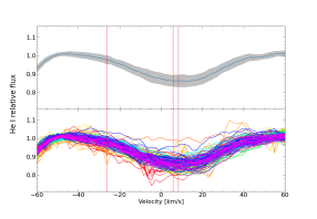
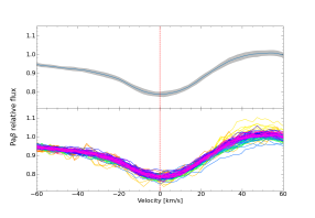
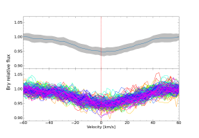
Figure 13: blackSpectra of V1298 Tau for the He i triplet (top), Pa$\beta$ (middle) and Br$\gamma$ (bottom). For each panel, the top curve shows the median profile with the dispersion in each velocity bin (in light grey) while the bottom curves depict the superposition of all individual telluric-corrected spectra. The red vertical dashed lines show the location of the lines. blackThe blue wing of Pa$\beta$ is likely blended with a Ca i line.

6 Summary and blackDiscussion

We presented the analysis of NIR spectropolarimetric blackobservations of V1298 Tau collected with SPIRou between 2019 Oct 02 and 2023 Feb 06, blackaimed at characterizing the large-scale magnetic topology of the host star and at further constraining the masses and densities of the 4 transiting planets.

6.1 Evolution of the magnetic field of V1298 Tau

Our Stokes $V$ LSD profiles show clear Zeeman signatures demonstrating that V1298 Tau hosts a strong large-scale magnetic field. The longitudinal field $B_{\ell}$, tracing this large-scale component, is modulated by the stellar rotation with a period of $2.910\pm 0.005$ d, blackconsistent with, though much more accurate than the estimate of $2.91\pm 0.05$ d inferred from RV measurements by Suárez Mascareño et al. (2021). $B_{\ell}$ evolves rapidly, over a time-scale of $36\pm 5$ d (the blackfull amplitude of the pattern varying from $\mathord{\sim}30$ G in 2020 to $\mathord{\sim}130$ G in 2021), suggesting that the large-scale magnetic topology changes both within an observing season and between two consecutive seasons.

Given the fast evolution of $B_{\ell}$, we split our data into several subsets per season on which ZDI was applied independently to reconstruct the large-scale magnetic topology of V1298 Tau. The large-scale magnetic topology of V1298 Tau is found to be mainly poloidal and axisymmetric with a toroidal component becoming less axisymmetric from 2020 to 2023. Comparing the magnetic reconstructions of this star with those of blacktwo young solar-mass stars similar to V1298 Tau, namely AB Dor (e.g. Donati et al. 2003b) and LQ Hya (e.g. Lehtinen et al. 2022), we find that V1298 Tau hosts a simpler large-scale magnetic field, with a mostly axisymmetric radial field mainly characterized by the dipole component of the poloidal field unlike both other stars. All three stars also continuously show azimuthal features at their surface, that blackmost likely indicate that the underlying dynamo processes operate throughout the entire convective zone of these stars, as suggested by Donati et al. (2003b). In addition, ZDI reconstructions from our latest blackobserving epoch show a rapid change in the radial field, with the dipole component (of the poloidal field) becoming much more tilted in early 2023 (from 20–30^∘ to 75^∘), blackand possibly tracing a polarity reversal, as blackthat recently reported for LQ Hya (Lehtinen et al., 2022). These changes blacksuggest that the magnetic field of V1298 Tau follows a long-term evolution blackpotentially similar to the 11-year solar cycle.

Part of the observed magnetic variability is likely blackattributable to DR at the surface of the star, found to be equal to black$82.0\pm 2.0$ $\rm mrad\,d^{-1}$, i.e. $\mathord{\sim}1.5$ times that of the Sun. This value implies a typical lap time of $\mathord{\sim}76$ d for the equator to lap the pole by one rotation, implying that DR clearly distorts the regular modulation of spectropolarimetric data over a typical observing season spanning about 4.5 months (i.e. $\mathord{\sim}135$ d, see Table 6). This level of DR is similar to that of young solar-mass stars whose stellar structure resembles that of V1298 Tau, such as AB Dor black(d$\Omega_{\rm ABDor}$ of the order of $70\,\mathrm{mrad\,d^{-1}}$; Jeffers et al. 2007) and LQ Hya (d$\Omega_{\rm LQHya}$ of the order of $100\,\mathrm{mrad\,d^{-1}}$; Donati et al. 2003b). In addition, our results suggest that the DR at the surface of V1298 Tau may be varying with time, blackpassing from $90.6\pm 2.8$ $\rm mrad\,d^{-1}$ in 2020 Aug - 2021 Jan to $73.5\pm 2.8$ $\rm mrad\,d^{-1}$ in 2021 Sep - 2022 Feb. This variation of $\mathord{\sim}15\,\mathrm{mrad\,d^{-1}}$ is larger than the one observed for the Sun ($<1~{}\mathrm{mrad\,d^{-1}}$) but is in good agreement with the observations of AB Dor and LQ Hya for which large variations of DR have also been reported from year to year, with, in particular, blackd$\Omega_{\rm ABDor}$ ranging from 60 to 75 $\rm mrad\,d^{-1}$ (Jeffers et al., 2007) and d$\Omega_{\rm LQHya}$ ranging from 14 to 200 $\rm mrad\,d^{-1}$ (Donati et al., 2003b; Kővári et al., 2004; Lehtinen et al., 2022). The global increase in the strength of the magnetic field of V1298 Tau between 2020 Aug - 2021 Jan and 2021 Sep - 2022 Feb (see the evolution of <$B_{V}$> in Sec. 3.2) may help to slow down the DR and may therefore contribute to the observed decrease in d$\Omega$ between both seasons. blackThe DR parameters of the Sun vary periodically with a period corresponding to that of the solar cycle and this peridocity is correlated with solar activity (Poljančić Beljan et al., 2022). However, with only two measurements of DR at the surface of V1298 Tau so far and no reported magnetic cycle, we cannot conclude whether DR parameters for V1298 Tau follow the same trend as those of the Sun.

We used, for the first time on actual data, the new tomographic method TIMeS (Finociety & Donati, 2022) allowing one to reconstruct the long-term temporal evolution of magnetic fields without splitting the whole data set. We fitted all the Stokes $V$ LSD profiles down to $\chi^{2}_{r}=1.49$, suggesting that discrepancies still exist between the synthetic model and the observed data. This is not surprising as Finociety & Donati (2022) mentioned in the original paper that the method is likely to miss the smallest features that only contribute little to the observed data. One major difference between TIMeS and ZDI is that the model derived with TIMeS only uses some spherical harmonics modes that strongly contribute to the magnetic topology over the whole time span of the observations to describe the magnetic field while the model derived with ZDI uses all spherical harmonic modes up to a maximum degree $\ell_{\rm max}$. We therefore suppose that the TIMeS method failed at fitting the data down to a unit $\chi^{2}_{r}$ because some high degree modes do not have a strong contribution to the magnetic field over all epochs (e.g. small features that may have a small lifetime) and they were therefore not selected for the model (only modes up to $\ell=4$ were indeed identified by the method). Future improvements of the method to increase the flexibility in the choice of the modes should help to reduce these discrepancies black(e.g. through new criteria of selection, implementation of DR in the model), but the results we obtained with this first application on real data are already quite promising. We indeed find an evolution of the magnetic topology with TIMeS similar to that reconstructed from the application of ZDI on data subsets. In addition, TIMeS allows one to access to the temporal evolution of the large-scale field and its decomposition into poloidal and toroidal components. Comparing the fraction of reconstructed magnetic energy enclosed in the poloidal field derived from ZDI and TIMeS, we see that we have a global consistency, except at some epochs blackat the beginning or end of a season black(typically 2021 Oct, 2023 Jan). To investigate whether we can distinguish a magnetic cycle within our data set, we computed periodograms of the coefficients reconstructed with TIMeS. We however do not see any significant period shared by all coefficients, and therefore conclude that, if this star has a magnetic cycle, it must be longer than the time span of our 2020-2023 observations (897 d, i.e. $\mathord{\sim}2.5$ years), as already suggested by the fact that only the beginning of a potential reversal has been identified in our ZDI reconstruction. Thorough spectropolarimetric monitorings of V1298 Tau are thus clearly needed in the blackcoming years, blackto help us identify whether the dynamo processes at work in this star are similar to blackthose operating in the Sun (e.g. $\alpha\Omega$ processes) or more complex blackones (e.g. $\alpha^{2}$, $\alpha^{2}\Omega$ processes, see Rincon 2019 for a review).

6.2 Constraining the planet parameters

Using the LBL method (Artigau et al., 2022), we computed 174 accurate RV values, over the 3.5 years of SPIRou monitoring, from which we estimated the mass and orbital period of the outermost planet (e) and upper limits on the mass of the three innermost planets. Assuming circular orbits, our SPIRou RV measurements yield 4 probable blackorbital periods for planet e at $42.7\pm 0.3$ d, $46.4\pm 0.4$ d, $53.5\pm 0.4$ d and $60.6\pm 0.7$ d. Computing the $\log{\mathcal{L_{M}}}$ associated with each model, we find that, among these solutions, the most likely model is the one featuring $P_{e}=53.5\pm 0.4$ d. We note that our best value disagrees with those found found by Sikora et al. (2023) and Turrini et al. (2023), equal to black$46.768131\pm 000076$ d and $45.46^{+1.10}_{-0.23}$ d, respectively, but these values remain compatible with one of our less likely solutions ($46.4\pm 0.3$ d) within $1\sigma$ and $2.4\sigma$, respectively. Although the log BF suggests that the period $P_{e}=42.7\pm 0.3$ d is the second most likely, we consider it to be less probable as this value corresponds to the lower limit provided by the TESS monitoring (Feinstein et al., 2022). We also consider that our largest period ($60.6\pm 0.7$ d) is also less probable given the log BF with respect to our best model ($\log{\rm BF}=-4.1$) and the most plausible interval ($43.3<P_{e}/\mathrm{d}<55.4$) derived by Sikora et al. (2023).

Using our most likely model, i.e. the one featuring a period of 53.5 d, we obtain the most significant detection of the RV signature of planet e since the new constraints on its orbital period provided by the TESS monitoring. We indeed report a 3.9$\sigma$ detection of the RV signature of planet e, yielding a mass of $1.01^{+0.35}_{-0.26}$ M_♃. This value is intermediate between those obtained by Sikora et al. (2023), Suárez Mascareño et al. (2021) and Turrini et al. (2023), equal to $0.66\pm 0.26$, $1.16\pm 0.30$ M_♃ and $1.23^{+0.35}_{-0.48}$ M_♃, respectively, but still compatible within $1\sigma$ with all values. From our mass value and the updated radius of planet e provided by Feinstein et al. (2022), we estimate the density of this planet to be equal to $1.79^{+0.66}_{-0.51}$ $\rm g\,cm^{-3}$, slightly lower than those given in Feinstein et al. (2022) and Turrini et al. (2023), using similar planet radius, but still compatible within $1\sigma$. As already noted by previous studies, this density is suprisingly high for a young planet, the implications of this value being discussed in the next Section.

The RV signatures of the three innermost planets are undetected from our SPIRou measurements. We therefore estimate the following upper limits on these masses, based on the 99% confidence interval of their posterior distributions sampled through the MCMC approach: $M_{b}<0.44$ M_♃, $M_{c}<0.22$ M_♃ and $M_{d}<0.25$ M_♃. These results illustrate the need for (i) powerful filtering methods to get rid of activity jitter in RV measurements to clearly unveil the planet properties and (ii) more observations to better sample the RV signature induced by each planet of this system.

blackOur results are generally consistent with those provided by Sikora et al. (2023) but less so with those of Suárez Mascareño et al. (2021). We outline that the masses derived by Suárez Mascareño et al. (2021) may be unreliable as a result of a potential overfit of their RV data as recently suggested by Blunt et al. (2023). Although our results do not allow us to strongly constrain the mass of the three innermost planets, we note that our estimate of $K_{b}=4.2\pm 10.7$ $\mathrm{m}\,\mathrm{s}^{-1}$ disagrees at a $\mathord{\sim}3\sigma$ level with the value of $41\pm 12$ $\mathrm{m}\,\mathrm{s}^{-1}$ previously reported in Suárez Mascareño et al. (2021), suggesting that planet b may be several times less massive. This result is further strengthened by the upper limit of 0.08 M_♃ provided by the HST transmission spectra of V1298 Tau b (Barat et al., submitted, 2023), fully consistent with our estimate of $M_{b}=0.07\pm 0.17$ M_♃.

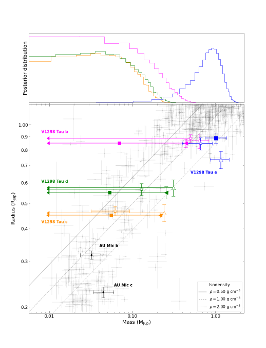
Figure 14: Mass-radius diagram. blackTop panel: Posterior distributions of the planet masses derived from the MCMC approach. V1298 Tau b, c, d and e are shown in magenta, orange, green and blue, respectively. Bottom panel: The light grey dots correspond to confirmed exoplanets with radius and masses known with a precision of 30% or lower. The full squares show the position of the 4 planets according to the mass and error bars derived in the present paper (assuming the radii of Feinstein et al. 2022), while the left-pointing triangles depict the upper limit associated with the 99% confidence level. The open up-pointing triangles show the estimates and $3\sigma$ upper limits from Suárez Mascareño et al. (2021) while the open stars correspond to recent estimates and $2\sigma$ upper limits from Sikora et al. (2023). Upper limits are identified by an arrow pointing to the left. The same color code as for the upper panel is used to identify the 4 planets. For comparison, the black dots correspond to the position of the two young planets AU Mic b and c from the estimates of Donati et al. (2023). We also plot 3 isodensities as thin grey lines, corresponding to a density of 0.50 (solid), 1.00 (dashed) and 2.00 (dotted) $\rm g\,cm^{-3}$.

Our estimate of planet c’s mass black($M_{c}=0.05\pm 0.07$ M_♃) is similar to the estimate of $19.8^{+9.3}_{-8.9}$ $M_{\oplus}$ black(i.e. $0.062^{+0.029}_{-0.028}$ M_♃) derived by Sikora et al. (2023), but with error bars $2.3\times$ larger, both results being fully consistent within $1\sigma$. Our RV data does not allow us to bring stronger constraints on the mass of planet d with respect to the previous studies, our upper limit being $\mathord{\sim}1.6\times$ larger than that of Sikora et al. (2023) but still $\mathord{\sim}1.6\times$ lower than that of Suárez Mascareño et al. (2021). The derived upper mass limits yield blackupper limits for the planet densities of $\rho_{b}<0.89$ $\rm g\,cm^{-3}$, $\rho_{c}<2.94$ $\rm g\,cm^{-3}$ and $\rho_{d}<1.89$ $\rm g\,cm^{-3}$. Future observations of V1298 Tau will help to refine these densities and suggest what their internal structures could be. To compare the results from both previous velocimetric studies and ours, we show the position of the four planets in a mass-radius diagram in Fig. 14.

We further confirm that the assumption of circular orbits is best adapted to model our RV data, in particular for planet e for which we derive an eccentricity consistent with 0 (with an error bar of 0.05).

Using the transit times of planet e derived from the K2 and TESS light curves Feinstein et al. (2022) listed 17 probable values for $P_{e}$ with a precision of 0.0001 d. We therefore used these values as a prior on $P_{e}$ for the modeling of our RV data. As outlined in Sec. 4.3, the models associated with these periods can be sorted according to the value of their $\log{\mathcal{L_{M}}}$. As expected from our main analysis, we find that, among these 17 periods, $P_{e}=53.0039\pm 0.0001$ d is the most likely, this value being the closest to our best period and consistent within 1.3$\sigma$. Three periods yield a $\log{\mathcal{L_{M}}}$ slightly smaller than that of the model featuring $P_{e}=53.0039$ d (i.e. $|\Delta\log{\mathcal{L_{M}}}|<2.5$). Among these 3 periods, one remains close to 53.5 d (i.e. $P_{e}=54.2085$ d) while the 2 others ($P_{e}=46.7681$ and $45.8687$ d) are in good agreement with one of the other solutions of our main analysis, i.e. $P_{e}=46.4\pm 0.4$. These results thus strengthen our blackinitial conclusion of an orbital period close to 53 d for the outermost planet of the V1298 Tau system. Future photometric transits of planet e are needed to further pinpoint whether its actual orbital period is $\mathord{\sim}46$ or $\mathord{\sim}53$ d.

With an orbital period of $P_{e}=53.0039$ d, the RV semi-amplitude of planet e is found to be equal to $K_{e}=44^{+15}_{-11}$ $\mathrm{m}\,\mathrm{s}^{-1}$, corresponding to a mass and density of $0.95^{+0.33}_{-0.24}$ M_♃ and $\rho_{e}=1.66^{+0.61}_{-0.48}$ $\rm g\,cm^{-3}$, respectively. These values are therefore fully consistent with and only sligthly lower than those derived blackin our main analysis, as expected from the blacksmall difference in the orbital period of planet e between both analyses.

6.3 Formation and evolution of the V1298 Tau system

According to the orbital periods of the four planets, the V1298 Tau system is likely not in a resonant chain blackwith only planet b, c and d having respective period ratios close to 3:2 (for c vs d) and 2:1 (for d vs b). A resonant chain would indeed favour an orbital period of planet e close to 48 or 49 d rather than 53 d (or even 46 d), which seems unlikely given our data (see Tables 10 and 11). Our finding is consistent with previous studies focussing on the formation of this planetary system (Tejada Arevalo et al., 2022; Turrini et al., 2023). This implies that either the V1298 Tau system did not form in a resonant chain, or if it did, it must have undergone a rapid phase of dynamical instabilities that broke the resonant chain after the disc dispersal (i.e. in 10-15 Myr given the young age of V1298 Tau).

blackAlthough theoretical models indicate that disc migration in a multiplanetary system tends to favour the planets to be in a resonant chain, several processes, such as planet-disc interactions, may prevent the formation of such chains (e.g. interaction between a planet and the wake of another one; Baruteau & Papaloizou 2013). We also outline that the turbulence of the circumstellar disc can play a role on the disc-planet interactions that eventually disrupt the strict mean motion resonance between the planets (Pierens et al., 2011; Paardekooper et al., 2013). Turrini et al. (2023) discussed several mechanisms that may break a resonant chain after its formation. The first one is the eccentricity damping through tidal dissipation (Batygin & Morbidelli, 2013) but this scenario seems unlikely as the timescale on which it would occur for planet c is 2 orders of magnitude larger than the age of the system (Turrini et al., 2023). Photoevaporation of planets c and d may also contribute to the break of resonance (Goldberg et al., 2022) but, once again, such a phenomenon would occur over more than 100 Myr, inconsistent with the age of the star (Turrini et al., 2023). More plausible explanations involve planetesimal scattering or planet-planet scattering. However, planetesimal scattering seems unlikely for this system as simulations show that a planetesimal belt of 50 $M_{\oplus}$ would not have a significant impact on the V1298 Tau system and a much more massive belt would be required to break the resonance (Turrini et al., 2023). Turrini et al. (2021) suggest that the most likely scenario to explain the non-resonance between planets b and e relates to planet-planet scattering, involving the presence of one or more planets on an eccentric orbit beyond the orbit of planet e. We however consider that this scenario is quite unlikely given that the eccentricity of planet e we derived from our data is consistent with 0. In addition, such additional planets would be difficult to detect through photometric transits and RV monitoring due to their long orbital periods. In particular, no hint of a fifth planet in this system has been reported so far and, using GAIA and SPHERE observations, Turrini et al. (2023) indicate that no planet more massive than $2$ M_♃ should orbit beyond 50 au from the host star (i.e. with an orbital period longer than 300 yr). blackFrom simulations, we also estimated that our data excludes the presence of planets more massive than 2.7 M_♃ and 5.9 M_♃ orbiting at 0.7 and 1.4 au (i.e. corresponding to orbital periods of 6 months or 1.5 yr), respectively, in good agreement with the results of Turrini et al. (2023) for similar orbital periods.

According to our best model, planet e has a suprisingly high density given its young age. In particular, the mass and density we derived for this planet are consistent with the plausible composition inferred by Sikora et al. (2023) from models of Fortney et al. (2007) accounting for the irradiation from a Sun-like host star at a distance of 0.1 au, i.e. a 100 $M_{\oplus}$ core composed of a 50/50 by mass ice-rock mixture surrounded by a H/He envelope. In addition, even though our derived mass is slightly lower than the one inferred from their recent study, Turrini et al. (2023) suggest that blackthe ice-rock core may be more massive than 100 $M_{\oplus}$ with about 2/3 of planet e composed of heavy elements and 1/3 of hydrogen and helium. This would mean a relative core mass $\mathord{\sim}6\times$ larger than that of Jupiter according to formation models (Venturini & Helled, 2020), i.e. a planet composition closer to that of Neptune than that of Jupiter. This result is in good agreement with the models of Baraffe et al. (2008), indicating that planet e should be composed of more than 50% of heavy elements (up to 90%) to match the measured radius (0.89 R_♃) at this young an age (10-15 Myr). blackHowever, these models predict that, assuming a metallicity of 0.10 (as in the host star; Suárez Mascareño et al. 2021), the planet should be blackolder than 10 Gyr given the measured radius, which is clearly unrealistic.

To date, the blackcause of such a high density of planet e is still speculative. One explanation blackrelates to the critical mass for the onset of runaway gas accretion onto a protoplanetary core. In the case of planet e, this mass would be larger than that generally admitted (10 to 20 $M_{\oplus}$) possibly due to uncertainties on the hypotheses on which models rely such as the size, mass and composition of the dust, having a direct impact on the opacity and on the cooling of the gas that can be accreted by the planet. Alternative explanations for the high density of V1298 Tau e may be related to a high accretion blackrate of pebbles, enriching the content of heavy elements of the planet, through different mechanisms. blackOne generally assumes that a planet on a circular orbit reaches its pebble isolation mass (PIM, i.e. the mass above which the planet cannot accrete more pebbles) for $M$ $\mathord{\sim}10-20~{}$ $M_{\oplus}$ depending on the disc’s aspect ratio around the planet (e.g., Ataiee et al., 2018). However, in some conditions, a planet on an eccentric orbit can reach a much higher PIM ($>100$ $M_{\oplus}$ for moderate eccentricity, e.g. $e>0.04$, and a turbulent visosity $\alpha=0.005$; Chametla et al. 2022), which could be the case of V1298 Tau e, according to the estimate we derived ($0.03\pm 0.05$). The accretion of dust and gas through a vertical (or meridional) circulation (Binkert et al., 2021; Szulágyi et al., 2022) is another process that can partly contribute to the increase in the heavy elements content in V1298 Tau e even if the planet has reached its PIM, that deserves to be further investigated.

Turrini et al. (2023), focussing on the evolution of the V1298 Tau system, also discussed other possible explanations for the high density observed for planet e. blackOne is that this planet formed beyond the CO₂ snowline and then underwent a large-scale migration within a massive circumstellar disc in such a way to accrete heavy elements along its pathway (as probably for HAT-P-20 b; Thorngren et al. 2016), e.g. through the accretion of an intense planetesimal flux preventing runaway accretion of the disc gas to occur (Turrini et al., 2023). As also noted by Turrini et al. (2023), another option is that this density results from an accretion of vapor coming from an enhancement of the volatile content of the circumstellar disc due to drifting and evaporating pebbles when they reach their ice lines (e.g. Booth & Ilee 2019; Schneider & Bitsch 2021). Characterizing the atmosphere of planet e through transit observations would help to discriminate between both hypotheses as the accretion of planetesimal is expected to yield a lower refractory-to-volatile ratio as well as a different C/O ratio than the second process (Turrini et al., 2021; Schneider & Bitsch, 2021; Pacetti et al., 2022). We however caution that these two processes blackmay not be consistent with what we know of V1298 Tau. In particular, the metallicity of the host star is close to solar ($0.10\pm 0.15$; Suárez Mascareño et al. 2021), and does not hint at a high content of heavy elements in the circumstellar disc that would lead towards the second hypothesis. Though much older ($\mathord{\sim}1.5$ Gyr; Ment et al. 2018), HAT-P-2 b ($M=8.62^{+0.39}_{-0.55}$ M_♃, $R=0.951^{+0.039}_{-0.053}$ R_♃; Loeillet et al. 2008) is another example of a hot Jupiter with an even higher density ($\rho=12.5^{+2.6}_{-3.6}$ $\rm g\,cm^{-3}$; Loeillet et al. 2008) that may be related to a large content of heavy elements (up to 500 $M_{\oplus}$; Baraffe et al. 2008). The most likely scenario to explain the formation of HAT-P-2 b is that the planet is actually the result of several collisions with planetary embryos (Baraffe et al., 2008). In this scenario, the absolute mass of heavy elements in the planet increases and the gas is ejected from the planet, therefore increasing the relative mass of heavy elements with respect to the initial mass of the planet. This mechanism may be an alternative explanation for the formation of V1298 Tau e, which deserves to be also investigated in future studies.

Maggio et al. (2022) mentioned that the two outermost planets (e and b) should not be affected by a strong photoevaporation given their large mass with respect to their radius. However, this conclusion was drawn from the mass of planet b inferred by Suárez Mascareño et al. (2021), blackwhich is larger than the upper limit that we report in the current paper and that of Sikora et al. (2023), blacksuggesting that the conclusion may be revised taking into account our updated mass upper limit. In addition, Turrini et al. (2023) indicate that, during its formation, planet b may have undergone a migration with heavy element enrichment (as for planet e). However, this conclusion was also drawn from a density derived assuming the mass obtained by Suárez Mascareño et al. (2021) and thus likely overestimated and inconsistent with our data. In particular, Turrini et al. (2023) suggest that planet b may contain up to 90 $M_{\oplus}$ (i.e. $\mathord{\sim}0.28$ M_♃) of heavy elements, blackrepresenting 64% of our mass upper limit (0.44 M_♃), which thus seems unlikely given our upper limit on the density of planet b ($<0.89$ $\rm g\,cm^{-3}$). The scenario for the formation of planet b can therefore be revised when the actual mass of this planet is further constrained.

According to Maggio et al. (2022), planets c and d may undergo strong atmospheric evaporation if their masses is lower than $\mathord{\sim}40$ $M_{\oplus}$ ($\mathord{\sim}0.13$ M_♃). blackOur mass estimates are thus in favour of strong atmospheric photoevaporation, strengthening the conclusion of Sikora et al. (2023) about planet c. blackThe V1298 Tau system, hosting 4 planets younger than 30 Myr, is an ideal laboratory to study star-planet interactions at early stages of the evolution. Future monitoring of this target will therefore help us to better understand the impact of such interactions on the formation and evolution of young planets.

blackIn a forthcoming work, we plan to couple all existing RV measurements (i.e. collected with HARPS-N, MAROON-X, SPIRou and HIRES; Suárez Mascareño et al. 2021; Sikora et al. 2023; Blunt et al. 2023) to perform a consistent analysis and hopefully to refine the planet masses. Such a study should include two potentially coupled GPs to simultaneously and consistently model the activity signals in the optical and NIR domains. In parallel, we will pursue our spectropolarimetric monitoring of V1298 Tau thanks to the SPICE Large Programme in the next semesters. In light of the results reported in the present paper, these future observations will help us to fulfill two major goals. The first one is to reconstruct the large-scale magnetic topology of the star using ZDI and TIMeS from new data to better characterize the dynamo process at the origin of the observed field and its evolution (e.g. potential magnetic cycle subject to $\alpha\Omega$ processes). The second goal is obviously to refine estimates of the mass of the four planets, but also to firmly ascertain the orbital period of planet e, a quite blackchallenging task given the amplitude of the stellar activity jitter more than $2.6\times$ larger than the semi-amplitude of the presumably blackmost massive planet (i.e. V1298 Tau e). Obtaining accurate measurements of the mass of the four planets of this system is an blackessential step to further constrain the mass-radius relation at early stages of evolution, as only blackfew other planets aged of less than 30 Myr have precise measured radius and mass (AU Mic b and c, HD 114082 b and HIP 67522 b; Donati et al. 2023; Zakhozhay et al. 2022; Rizzuto et al. 2020), but also to better understand the evolution of young planets and the associated star-planet interaction. Coupling spectroscopic and high-precision photometric observations (e.g. TESS, PLATO), especially during transit events, will clearly help us to refine the orbital parameters, the atmospheric escape, if any, (e.g. study of the He i line during transit events) and the mass of the 4 planets. More generally, we would need multi-instruments campaigns (e.g. combination of optical/NIR spectropolarimeters, such as ESPaDOnS, SPIRou, CRIRES+) would provide huge benefits to better characterize the magnetic topology of V1298 Tau and the properties of its planetary system.

Data Availability

The data collected in the framework of the SLS will be publicly available from the Canadian Astronomy Data Center (CADC) by 2024, while the PI data are already public.

Appendix A Journals of observations

We provide a full journal of the observations reduced with the Libre-ESpRIT pipeline adapted for SPIRou in Table 6 and the journals of observations reduced with APERO in Tables 9.

Table 6: Spectropolarimetric observations collected between 2019 and 2023, reduced with the Libre-ESpRIT pipeline adapted for SPIRou data. For each observation, we list the date (day, hour), the barycentric Julian date (BJD), the rotation cycle (as defined in Sec. 3.2), the SNR in the $H$ band, the noise level in the LSD profile, the longitudinal field $B_{\ell}$ and the number of the subset used in ZDI (see Sec. 3.2).

Date	UTC	BJD	Cycle	SNR	$\sigma_{V}$	$B_{\ell}$	# ZDI
		2459000+			($10^{-4}\,I_{c}$)	(G)
2019 Oct 02	13:36:45	-240.92942	-82.794	160	3.17	$-9.4\pm 14.2$	1
2019 Oct 03	13:57:59	-239.91458	-82.445	161	2.85	$2.0\pm 13.2$	1
2019 Oct 05	11:03:45	-238.03544	-81.799	176	2.64	$8.1\pm 11.8$	1
2019 Oct 06	10:49:33	-237.04522	-81.459	184	2.72	$-7.6\pm 12.0$	1
2019 Oct 07	14:52:09	-235.87667	-81.057	139	3.75	$51.0\pm 16.3$	1
2019 Oct 08	09:24:54	-235.10387	-80.792	171	3.33	$-6.6\pm 14.1$	1
2019 Oct 09	12:11:43	-233.98794	-80.408	164	2.99	$1.4\pm 13.1$	1
2019 Oct 12	11:46:45	-231.00506	-79.383	170	2.68	$7.0\pm 12.0$	1
2019 Oct 13	14:06:44	-229.90778	-79.006	170	2.77	$88.8\pm 12.5$	1
2019 Oct 14	11:09:21	-229.03090	-78.705	170	2.85	$-55.9\pm 12.6$	1
2019 Oct 15	12:57:33	-227.95569	-78.335	161	3.30	$-33.0\pm 14.3$	1
2019 Oct 16	11:07:36	-227.03199	-78.018	185	2.85	$47.2\pm 12.6$	1
2019 Oct 31	10:50:51	-212.04282	-72.867	139	4.01	$10.5\pm 17.4$	2
2019 Nov 01	11:04:03	-211.03361	-72.520	177	3.05	$15.2\pm 13.3$	2
2019 Nov 03	10:19:43	-209.06433	-71.843	176	2.92	$-19.9\pm 12.7$	2
2019 Nov 04	11:29:17	-208.01597	-71.483	123	4.53	$34.2\pm 19.4$	2
2019 Nov 05	13:44:58	-206.92171	-71.107	162	3.22	$-21.6\pm 14.2$	2
2019 Nov 07	10:27:08	-205.05904	-70.467	144	4.25	$-1.1\pm 17.9$	2
2019 Nov 08	12:25:03	-203.97711	-70.095	159	3.34	$2.8\pm 14.5$	2
2019 Nov 09	09:37:13	-203.09364	-69.792	139	4.27	$-30.8\pm 18.0$	2
2019 Nov 10	10:19:47	-202.06405	-69.438	156	3.93	$23.7\pm 16.5$	2
2019 Nov 11	10:06:46	-201.07307	-69.097	165	3.48	$-10.9\pm 14.8$	2
2019 Nov 13	09:12:58	-199.11039	-68.423	170	3.26	$7.2\pm 14.0$	2
2019 Nov 14	09:36:55	-198.09374	-68.073	171	2.99	$-40.4\pm 13.1$	2
2019 Dec 07	09:52:47	-175.08273	-60.166	80	7.52	$-3.3\pm 32.2$	2
2019 Dec 08	08:47:45	-174.12792	-59.838	145	3.71	$12.7\pm 16.0$	2
2019 Dec 09	08:59:53	-173.11951	-59.491	157	3.13	$18.4\pm 13.8$	2
2019 Dec 10	07:53:49	-172.16542	-59.163	181	2.68	$-4.7\pm 11.7$	2
2019 Dec 11	10:42:40	-171.04819	-58.779	145	3.61	$6.4\pm 15.3$	2
2019 Dec 12	09:00:04	-170.11947	-58.460	151	2.84	$25.2\pm 12.7$	2
2019 Dec 13	08:38:10	-169.13471	-58.122	107	5.89	$-39.3\pm 23.9$	2
2020 Feb 05	05:27:09	-115.27106	-39.612	161	2.51	$9.9\pm 11.1$	-
2020 Feb 06	05:54:59	-114.25182	-39.262	102	5.92	$-4.6\pm 25.1$	-
2020 Feb 16	05:23:19	-104.27480	-35.833	152	3.06	$-32.6\pm 13.5$	-
2020 Feb 17	05:30:02	-103.27023	-35.488	132	4.26	$1.4\pm 17.9$	-
2020 Feb 18	05:26:10	-102.27301	-35.145	175	2.78	$-24.4\pm 12.1$	-
2020 Feb 19	05:25:58	-101.27325	-34.802	180	2.63	$-31.5\pm 11.6$	-
2020 Aug 26	14:42:57	88.11322	30.279	197	2.34	$-12.5\pm 10.8$	3
2020 Aug 27	13:33:22	89.06498	30.607	234	1.92	$-50.5\pm 8.9$	3
2020 Aug 28	13:34:37	90.06596	30.951	221	1.80	$-3.0\pm 8.5$	3
2020 Aug 29	14:29:19	91.10404	31.307	212	1.92	$-20.9\pm 8.9$	3
2020 Aug 30	14:13:30	92.09315	31.647	224	1.94	$-44.5\pm 8.9$	3
2020 Aug 31	14:17:54	93.09630	31.992	194	1.84	$15.5\pm 8.6$	3
2020 Sep 01	14:29:26	94.10442	32.338	192	1.87	$-45.8\pm 8.9$	3
2020 Sep 02	14:39:14	95.11132	32.684	214	1.91	$-58.8\pm 8.9$	3
2020 Sep 03	14:34:19	96.10800	33.027	178	2.53	$34.9\pm 11.7$	3
2020 Sep 04	14:18:22	97.09702	33.367	211	2.21	$-31.4\pm 9.9$	3
2020 Sep 05	14:20:39	98.09870	33.711	212	2.03	$-57.5\pm 9.3$	3
2020 Sep 06	13:54:00	99.08029	34.048	215	1.94	$15.2\pm 9.0$	3
2020 Sep 07	15:21:37	100.14124	34.413	171	2.71	$-46.7\pm 12.5$	3
2020 Sep 08	13:49:35	101.07742	34.735	221	1.93	$-60.8\pm 8.9$	3
2020 Sep 09	13:24:07	102.05982	35.072	210	2.16	$8.4\pm 9.9$	3
2020 Sep 10	13:23:01	103.05916	35.416	218	1.94	$-32.8\pm 8.9$	3

Table 7: Continued

Date	UTC	BJD	Cycle	SNR	$\sigma_{V}$	$B_{\ell}$	# ZDI
		2459000+			($10^{-4}\,I_{c}$)	(G)
2020 Sep 18	12:36:29	111.02759	38.154	203	2.63	$-2.4\pm 11.4$	4
2020 Sep 19	13:35:35	112.06872	38.512	182	3.25	$11.5\pm 14.7$	4
2020 Sep 20	14:03:47	113.08839	38.862	226	1.82	$-14.4\pm 8.5$	4
2020 Sep 21	11:48:57	113.99484	39.173	192	2.27	$0.7\pm 10.5$	4
2020 Sep 22	12:15:13	115.01317	39.523	220	2.12	$-9.2\pm 9.5$	4
2020 Sep 23	13:14:26	116.05438	39.881	206	2.15	$-6.2\pm 9.8$	4
2020 Sep 25	12:40:16	118.03083	40.560	239	1.82	$-6.0\pm 8.4$	4
2020 Sep 26	13:12:27	119.05327	40.912	232	1.73	$-4.9\pm 8.2$	4
2020 Sep 27	12:34:52	120.02724	41.246	226	1.90	$-5.3\pm 8.8$	4
2020 Sep 28	11:02:51	120.96342	41.568	234	1.88	$-2.7\pm 8.7$	4
2020 Sep 29	13:29:38	122.06545	41.947	232	1.90	$3.2\pm 8.8$	4
2020 Sep 30	10:52:30	122.95640	42.253	232	2.00	$-24.8\pm 8.9$	4
2020 Oct 01	13:12:29	124.05370	42.630	184	2.69	$8.6\pm 11.9$	4
2020 Oct 03	14:46:34	126.11920	43.340	220	2.00	$-24.3\pm 9.2$	4
2020 Oct 04	11:06:44	126.96660	43.631	226	2.08	$1.6\pm 9.4$	4
2020 Oct 05	10:28:17	127.93997	43.966	236	2.02	$-12.7\pm 9.1$	4
2020 Oct 07	10:17:42	129.93278	44.650	217	2.06	$-6.3\pm 9.3$	4
2020 Oct 08	13:07:34	131.05082	45.035	209	2.22	$-35.2\pm 10.1$	4
2020 Oct 30	12:18:21	153.01791	52.583	221	1.93	$33.9\pm 8.9$	-
2020 Oct 31	12:50:06	154.04002	52.935	243	1.67	$-5.1\pm 7.9$	-
2020 Nov 01	09:56:44	154.91965	53.237	252	1.75	$-22.5\pm 8.0$	-
2020 Nov 03	10:47:20	156.95487	53.936	232	2.02	$-9.7\pm 9.1$	-
2020 Nov 04	10:53:09	157.95894	54.281	216	2.17	$-22.6\pm 9.8$	-
2020 Nov 05	09:00:19	158.88062	54.598	233	2.07	$25.9\pm 9.3$	-
2020 Dec 24	08:17:18	207.85031	71.426	209	2.04	$-0.6\pm 9.3$	5
2020 Dec 25	08:32:59	208.86115	71.774	222	2.07	$17.7\pm 9.3$	5
2020 Dec 26	07:58:47	209.83735	72.109	222	2.14	$-65.3\pm 9.7$	5
2020 Dec 28	08:59:53	211.87967	72.811	146	4.34	$-3.2\pm 19.2$	5
2020 Dec 29	08:32:00	212.86025	73.148	173	3.07	$-54.4\pm 13.5$	5
2020 Dec 30	08:25:44	213.85584	73.490	207	2.40	$12.5\pm 10.8$	5
2020 Dec 31	08:11:27	214.84586	73.830	203	2.47	$-1.8\pm 11.1$	5
2021 Jan 01	06:58:05	215.79486	74.156	198	2.51	$-33.0\pm 11.2$	5
2021 Jan 02	07:26:51	216.81477	74.507	210	2.04	$22.3\pm 9.2$	5
2021 Jan 03	07:58:28	217.83666	74.858	223	1.87	$-2.8\pm 8.7$	5
2021 Jan 04	07:08:44	218.80206	75.190	235	1.86	$-31.4\pm 8.4$	5
2021 Jan 05	07:41:19	219.82462	75.541	218	1.98	$0.1\pm 9.2$	5
2021 Jan 06	07:15:27	220.80659	75.879	221	2.05	$-11.1\pm 9.4$	5
2021 Jan 07	07:37:07	221.82157	76.227	211	2.22	$-57.5\pm 10.1$	5
2021 Jan 08	07:46:46	222.82820	76.573	206	2.17	$-7.7\pm 10.0$	5
2021 Sep 17	13:43:20	475.07388	163.256	234	2.07	$-67.2\pm 9.3$	-
2021 Sep 19	11:59:44	477.00211	163.918	223	1.89	$-41.6\pm 8.6$	-
2021 Sep 22	13:05:24	480.04798	164.965	215	1.82	$0.7\pm 8.5$	-
2021 Sep 23	13:30:54	481.06578	165.315	219	1.93	$-64.0\pm 8.8$	-
2021 Sep 24	13:30:41	482.06572	165.658	208	1.88	$-62.9\pm 8.7$	-
2021 Oct 14	11:50:19	501.99755	172.508	210	2.32	$-14.0\pm 10.3$	6
2021 Oct 15	11:28:00	502.98211	172.846	227	1.98	$-43.3\pm 9.1$	6
2021 Oct 16	12:21:26	504.01928	173.203	203	2.27	$-32.3\pm 10.3$	6
2021 Oct 19	13:05:35	507.05014	174.244	240	2.05	$-22.8\pm 9.1$	6
2021 Oct 20	11:45:53	507.99484	174.569	228	2.08	$-25.1\pm 9.3$	6
2021 Oct 21	12:06:24	509.00915	174.917	226	2.24	$13.9\pm 9.9$	6
2021 Oct 22	12:07:18	510.00982	175.261	168	2.78	$-2.9\pm 12.3$	6
2021 Oct 23	11:51:29	510.99890	175.601	248	1.87	$-58.8\pm 8.4$	6
2021 Oct 24	12:30:07	512.02578	175.954	177	2.88	$22.3\pm 12.7$	6
2021 Oct 25	09:28:49	512.89993	176.254	243	1.88	$-22.4\pm 8.6$	6
2021 Oct 26	11:13:30	513.97267	176.623	240	1.98	$-60.9\pm 8.9$	6
2021 Oct 27	11:57:19	515.00315	176.977	216	2.06	$60.7\pm 9.3$	6
2021 Oct 28	12:28:43	516.02500	177.328	196	2.30	$-33.8\pm 10.5$	6

Table 8: Continued

Date	UTC	BJD	Cycle	SNR	$\sigma_{V}$	$B_{\ell}$	# ZDI
		2459000+			($10^{-4}\,I_{c}$)	(G)
2021 Nov 19	10:35:48	537.94721	184.862	203	2.16	$-35.1\pm 9.7$	7
2021 Nov 20	10:11:48	538.93054	185.199	229	1.84	$-22.5\pm 8.4$	7
2021 Nov 21	10:18:53	539.93548	185.545	197	1.96	$-48.1\pm 9.0$	7
2021 Nov 22	10:53:29	540.95951	185.897	231	1.87	$-15.3\pm 8.6$	7
2021 Dec 09	09:20:44	557.89492	191.716	216	2.10	$-85.6\pm 9.5$	7
2021 Dec 10	08:45:09	558.87018	192.052	230	1.92	$26.0\pm 8.7$	7
2021 Dec 11	08:49:02	559.87286	192.396	206	2.37	$-57.4\pm 10.7$	7
2021 Dec 12	08:54:58	560.87694	192.741	199	2.36	$-40.6\pm 10.7$	7
2021 Dec 13	09:28:59	561.90053	193.093	158	3.26	$12.2\pm 14.5$	7
2021 Dec 14	07:38:37	562.82387	193.410	231	1.97	$-28.8\pm 9.0$	7
2021 Dec 16	11:02:16	564.96521	194.146	170	2.96	$11.2\pm 13.2$	7
2021 Dec 18	08:40:17	566.86653	194.799	175	2.87	$-50.5\pm 12.7$	7
2022 Jan 06	08:34:54	585.86176	201.327	235	2.30	$-43.2\pm 10.4$	8
2022 Jan 08	08:15:43	587.84829	202.010	238	1.89	$44.3\pm 8.7$	8
2022 Jan 09	08:17:20	588.84935	202.354	234	2.00	$-57.5\pm 9.1$	8
2022 Jan 10	09:26:45	589.89748	202.714	238	2.06	$-71.5\pm 9.5$	8
2022 Jan 12	08:52:09	591.87330	203.393	241	1.84	$-75.1\pm 8.4$	8
2022 Jan 13	08:20:54	592.85153	203.729	236	1.97	$-43.5\pm 8.6$	8
2022 Jan 14	06:59:34	593.79498	204.053	219	2.11	$42.2\pm 9.4$	8
2022 Jan 15	08:36:53	594.86247	204.420	247	1.87	$-82.1\pm 8.4$	8
2022 Jan 17	06:50:18	596.78831	205.082	209	2.05	$34.6\pm 9.2$	8
2022 Jan 18	07:58:19	597.83545	205.442	239	1.81	$-92.9\pm 8.3$	8
2022 Jan 19	07:40:35	598.82305	205.781	225	2.05	$-18.6\pm 9.3$	8
2022 Jan 20	07:22:44	599.81058	206.120	224	2.24	$0.1\pm 10.2$	8
2022 Jan 21	08:13:25	600.84569	206.476	239	2.23	$-87.3\pm 10.0$	8
2022 Jan 22	07:18:30	601.80746	206.807	165	3.07	$-16.7\pm 13.8$	8
2022 Jan 23	08:11:59	602.84451	207.163	193	3.12	$-3.8\pm 13.8$	8
2022 Jan 24	07:43:09	603.82441	207.500	240	1.83	$-91.5\pm 8.4$	8
2022 Jan 25	07:51:28	604.83009	207.845	219	2.02	$-14.1\pm 9.3$	8
2022 Jan 26	06:58:15	605.79305	208.176	160	3.20	$-1.8\pm 14.3$	8
2022 Jan 27	07:00:00	606.79418	208.520	211	2.41	$-112.2\pm 11.0$	8
2022 Jan 28	07:00:14	607.79425	208.864	108	3.98	$-15.4\pm 17.8$	8
2022 Jan 29	06:50:19	608.78727	209.205	199	2.19	$-33.8\pm 10.0$	8
2022 Jan 30	07:04:52	609.79728	209.552	235	1.94	$-114.6\pm 9.0$	8
2022 Nov 02	13:01:59	886.04829	304.484	238	1.65	$-26.1\pm 7.7$	9
2022 Nov 06	12:18:09	890.01799	305.848	219	2.04	$-30.9\pm 9.4$	9
2022 Nov 07	12:36:23	891.03068	306.196	225	1.91	$-31.2\pm 8.9$	9
2022 Nov 08	12:43:07	892.03538	306.541	202	2.23	$-29.1\pm 10.2$	9
2022 Nov 09	13:06:42	893.05179	306.891	208	2.12	$-32.3\pm 9.8$	9
2022 Nov 10	14:29:05	894.10903	307.254	189	2.50	$-52.9\pm 11.4$	9
2022 Nov 11	13:31:54	895.06934	307.584	207	2.07	$-19.0\pm 9.6$	9
2022 Nov 12	10:27:35	895.94137	307.884	253	1.64	$-56.1\pm 7.6$	9
2022 Nov 14	10:39:27	897.94965	308.574	208	1.96	$-21.7\pm 9.1$	9
2022 Nov 16	13:32:58	900.07018	309.302	228	1.85	$-44.5\pm 8.6$	9
2022 Nov 17	12:54:51	901.04373	309.637	240	1.70	$-23.7\pm 7.8$	9
2022 Nov 18	13:52:13	902.08358	309.994	222	1.92	$-10.7\pm 8.9$	9
2022 Nov 21	12:43:21	905.03577	311.009	197	2.17	$-18.9\pm 10.1$	9
2022 Dec 01	10:31:23	914.94412	314.414	245	1.83	$-59.6\pm 8.1$	9
2022 Dec 02	14:00:46	916.08950	314.807	240	1.81	$-60.0\pm 8.3$	9
2022 Dec 03	11:47:38	916.99703	315.119	249	1.78	$6.0\pm 8.0$	9
2022 Dec 30	11:08:30	943.96886	324.388	246	1.85	$-7.7\pm 8.3$	10
2023 Jan 01	09:20:08	945.89349	325.049	230	1.86	$-13.1\pm 8.6$	10
2023 Jan 02	10:34:18	946.94493	325.411	234	1.89	$-13.8\pm 8.8$	10
2023 Jan 04	09:33:26	948.90254	326.083	243	1.63	$-6.3\pm 7.6$	10
2023 Jan 05	10:02:50	949.92289	326.434	212	2.15	$6.9\pm 9.7$	10
2023 Jan 06	07:22:54	950.81176	326.739	210	2.09	$-17.1\pm 9.5$	10
2023 Jan 07	07:49:05	951.82987	327.089	191	2.48	$10.3\pm 11.1$	10
2023 Jan 08	08:13:35	952.84681	327.439	222	1.96	$8.8\pm 8.9$	10
2023 Jan 09	10:17:58	953.93312	327.812	237	1.84	$-37.2\pm 8.3$	10
2023 Jan 10	09:49:31	954.91329	328.149	232	1.92	$21.3\pm 8.8$	10
2023 Jan 12	08:00:02	956.83712	328.810	240	1.77	$-22.5\pm 8.3$	10
2023 Jan 13	09:03:30	957.88112	329.169	240	1.90	$17.1\pm 8.6$	10
2023 Feb 02	08:05:52	977.83937	336.027	243	1.88	$-23.8\pm 8.4$	10
2023 Feb 03	07:57:59	978.83380	336.369	243	1.87	$-2.7\pm 8.3$	10
2023 Feb 06	06:57:19	981.79138	337.385	220	2.19	$-9.4\pm 9.7$	10
2023 Feb 09	07:11:40	984.80106	338.420	217	2.08	$-1.1\pm 9.5$	10

Table 9: Spectropolarimetric observations collected between 2019 and 2023, reduced with the APERO pipeline. For each observation, we list the date, the barycentric Julian date (BJD) and the associated RV computed from the LBL approach of Artigau et al. (2022).

Date	BJD	RV	Date	BJD	RV	Date	BJD	RV
	+2459000	($\mathrm{m\,s^{-1}}$)		+2459000	($\mathrm{m\,s^{-1}}$)		+2459000	($\mathrm{m\,s^{-1}}$)
2019 Oct 02	-240.92770	$-173.0\pm 19.7$	2020 Sep 26	119.05388	$-257.4\pm 12.8$	2021 Dec 13	561.90135	$100.1\pm 18.8$
2019 Oct 03	-239.91417	$3.3\pm 19.4$	2020 Sep 27	120.02753	$-183.5\pm 13.9$	2021 Dec 14	562.82473	$-26.3\pm 13.1$
2019 Oct 05	-238.03456	$-78.0\pm 17.3$	2020 Sep 28	120.96423	$58.1\pm 13.0$	2021 Dec 16	564.96708	$-141.4\pm 17.2$
2019 Oct 06	-237.04434	$35.4\pm 18.0$	2020 Sep 29	122.06575	$-164.9\pm 13.3$	2021 Dec 18	566.86757	$201.9\pm 17.3$
2019 Oct 07	-235.87655	$49.6\pm 23.3$	2020 Sep 30	122.95714	$-39.3\pm 14.2$	2022 Jan 06	585.86248	$-155.9\pm 13.0$
2019 Oct 08	-235.10344	$-140.6\pm 20.2$	2020 Oct 01	124.05417	$14.2\pm 16.1$	2022 Jan 08	587.84907	$105.6\pm 12.1$
2019 Oct 09	-233.98644	$-33.4\pm 18.9$	2020 Oct 03	126.11995	$-156.9\pm 13.6$	2022 Jan 09	588.85007	$-132.8\pm 12.8$
2019 Oct 12	-231.00453	$-93.9\pm 18.2$	2020 Oct 04	126.96732	$-51.8\pm 13.1$	2022 Jan 10	589.89933	$-157.0\pm 15.7$
2019 Oct 13	-229.90697	$-19.6\pm 18.7$	2020 Oct 05	127.94074	$-170.4\pm 13.6$	2022 Jan 12	591.87405	$-89.7\pm 12.1$
2019 Oct 14	-229.03016	$-94.1\pm 18.6$	2020 Oct 07	129.93348	$-24.8\pm 13.8$	2022 Jan 13	592.85215	$100.4\pm 12.6$
2019 Oct 15	-227.95457	$-8.9\pm 20.2$	2020 Oct 08	131.05194	$116.3\pm 13.5$	2022 Jan 14	593.79602	$41.5\pm 12.4$
2019 Oct 16	-227.03129	$-18.2\pm 19.1$	2020 Oct 30	153.01912	$185.1\pm 13.1$	2022 Jan 15	594.86326	$-16.7\pm 12.8$
2019 Oct 31	-212.04262	$-105.8\pm 22.5$	2020 Oct 31	154.04080	$-77.9\pm 12.3$	2022 Jan 17	596.78913	$25.9\pm 12.7$
2019 Nov 01	-211.03317	$43.3\pm 18.0$	2020 Nov 01	154.92044	$88.7\pm 12.5$	2022 Jan 18	597.83624	$29.4\pm 12.3$
2019 Nov 03	-209.06372	$-77.7\pm 18.2$	2020 Nov 03	156.95591	$-22.7\pm 13.4$	2022 Jan 19	598.82397	$115.0\pm 12.9$
2019 Nov 04	-207.98978	$201.1\pm 18.8$	2020 Nov 04	157.95988	$-16.0\pm 14.2$	2022 Jan 20	599.81147	$34.3\pm 12.9$
2019 Nov 05	-206.92075	$52.8\pm 20.4$	2020 Nov 05	158.88105	$154.7\pm 14.0$	2022 Jan 21	600.84655	$-95.5\pm 12.9$
2019 Nov 07	-205.05744	$184.4\pm 22.7$	2020 Dec 24	207.85127	$120.6\pm 12.9$	2022 Jan 22	601.80756	$72.3\pm 17.7$
2019 Nov 08	-203.97627	$102.2\pm 20.6$	2020 Dec 25	208.86203	$-170.1\pm 13.9$	2022 Jan 23	602.84476	$-142.5\pm 15.5$
2019 Nov 09	-203.09302	$-192.6\pm 22.8$	2020 Dec 26	209.83772	$180.4\pm 13.2$	2022 Jan 24	603.82528	$-129.6\pm 12.8$
2019 Nov 10	-202.06264	$90.3\pm 21.2$	2020 Dec 28	211.88035	$-217.3\pm 21.4$	2022 Jan 25	604.83094	$130.5\pm 13.0$
2019 Nov 11	-201.07236	$43.8\pm 21.2$	2020 Dec 29	212.86158	$200.8\pm 17.2$	2022 Jan 26	605.79593	$-128.0\pm 17.0$
2019 Nov 13	-199.10934	$56.3\pm 19.5$	2020 Dec 30	213.85724	$200.4\pm 14.4$	2022 Jan 27	606.79591	$-111.5\pm 14.1$
2019 Nov 14	-198.09287	$-34.0\pm 19.3$	2020 Dec 31	214.84685	$-176.2\pm 14.7$	2022 Jan 28	607.79565	$16.7\pm 21.1$
2019 Dec 08	-174.12800	$24.6\pm 21.9$	2021 Jan 01	215.79469	$178.7\pm 14.9$	2022 Jan 29	608.78903	$-180.4\pm 14.1$
2019 Dec 09	-173.11839	$245.4\pm 19.8$	2021 Jan 02	216.81589	$225.8\pm 12.8$	2022 Jan 30	609.79823	$-117.0\pm 12.7$
2019 Dec 10	-172.16480	$104.7\pm 17.9$	2021 Jan 03	217.83753	$-312.0\pm 12.7$	2022 Nov 02	886.04909	$-193.1\pm 12.9$
2019 Dec 11	-171.04722	$-235.8\pm 20.8$	2021 Jan 04	218.80285	$128.6\pm 12.6$	2022 Nov 06	890.01754	$115.0\pm 14.2$
2019 Dec 12	-170.11785	$160.8\pm 18.3$	2021 Jan 05	219.82561	$169.8\pm 12.6$	2022 Nov 07	891.03186	$175.0\pm 13.5$
2020 Feb 05	-115.26991	$-209.2\pm 16.8$	2021 Jan 06	220.80741	$-231.7\pm 12.4$	2022 Nov 08	892.03611	$-86.5\pm 14.8$
2020 Feb 06	-114.25273	$64.1\pm 26.6$	2021 Jan 07	221.82268	$70.6\pm 13.3$	2022 Nov 09	893.05207	$17.5\pm 14.3$
2020 Feb 16	-104.27375	$-268.7\pm 20.3$	2021 Jan 08	222.82881	$81.0\pm 13.3$	2022 Nov 10	894.10944	$12.7\pm 16.8$
2020 Feb 17	-103.25826	$-84.4\pm 17.9$	2021 Sep 17	475.07447	$-44.8\pm 13.8$	2022 Nov 11	895.07057	$0.3\pm 14.2$
2020 Feb 18	-102.27201	$-253.8\pm 18.9$	2021 Sep 19	477.00284	$76.1\pm 14.6$	2022 Nov 12	895.94206	$85.1\pm 11.9$
2020 Feb 19	-101.27236	$-320.1\pm 19.4$	2021 Sep 22	480.04888	$-16.4\pm 13.1$	2022 Nov 14	897.95194	$18.1\pm 12.7$
2020 Aug 26	88.11057	$103.5\pm 14.3$	2021 Sep 23	481.06655	$-72.9\pm 13.1$	2022 Nov 16	900.07114	$-86.4\pm 12.9$
2020 Aug 27	89.06586	$137.5\pm 12.8$	2021 Sep 24	482.06653	$52.0\pm 12.6$	2022 Nov 17	901.04443	$-34.2\pm 12.2$
2020 Aug 28	90.06677	$129.8\pm 13.5$	2021 Oct 14	501.99866	$-124.4\pm 14.4$	2022 Nov 18	902.08416	$51.8\pm 13.8$
2020 Aug 29	91.10476	$94.8\pm 13.0$	2021 Oct 15	502.98309	$-46.5\pm 13.5$	2022 Nov 21	905.03656	$48.6\pm 14.7$
2020 Aug 30	92.09409	$113.5\pm 12.9$	2021 Oct 16	504.02054	$-18.0\pm 13.5$	2022 Dec 01	914.94482	$-198.2\pm 12.5$
2020 Aug 31	93.09734	$180.6\pm 13.8$	2021 Oct 19	507.05093	$-37.0\pm 12.9$	2022 Dec 02	916.09044	$101.6\pm 12.9$
2020 Sep 01	94.10528	$-21.6\pm 13.9$	2021 Oct 20	507.99552	$14.0\pm 13.6$	2022 Dec 03	916.99788	$123.5\pm 12.0$
2020 Sep 02	95.11229	$161.8\pm 13.4$	2021 Oct 21	509.01032	$38.8\pm 13.6$	2022 Dec 30	943.96972	$2.2\pm 12.8$
2020 Sep 03	96.10971	$32.7\pm 15.9$	2021 Oct 22	510.01080	$-20.0\pm 16.7$	2023 Jan 01	945.89484	$61.0\pm 12.7$
2020 Sep 04	97.09765	$-9.9\pm 15.2$	2021 Oct 23	510.99954	$116.6\pm 13.2$	2023 Jan 02	946.94596	$-16.3\pm 13.1$
2020 Sep 05	98.09947	$141.5\pm 13.3$	2021 Oct 24	512.02744	$26.7\pm 15.9$	2023 Jan 04	948.90342	$55.6\pm 12.3$
2020 Sep 06	99.08083	$-10.6\pm 13.2$	2021 Oct 25	512.90057	$145.1\pm 12.5$	2023 Jan 05	949.92427	$-93.1\pm 13.8$
2020 Sep 07	100.14238	$20.5\pm 17.1$	2021 Oct 26	513.97343	$130.4\pm 12.5$	2023 Jan 06	950.81330	$216.8\pm 13.7$
2020 Sep 08	101.07823	$78.9\pm 13.0$	2021 Oct 27	515.00383	$111.1\pm 12.6$	2023 Jan 07	951.83052	$102.0\pm 15.8$
2020 Sep 09	102.06046	$90.1\pm 14.1$	2021 Oct 28	516.02592	$-162.9\pm 14.4$	2023 Jan 08	952.84767	$-139.8\pm 12.9$
2020 Sep 10	103.06001	$-20.5\pm 13.0$	2021 Nov 19	537.94856	$147.1\pm 13.0$	2023 Jan 09	953.93397	$135.5\pm 12.6$
2020 Sep 18	111.02850	$13.9\pm 16.0$	2021 Nov 20	538.93158	$-90.4\pm 12.3$	2023 Jan 10	954.91419	$65.9\pm 12.8$
2020 Sep 19	112.06913	$38.3\pm 17.4$	2021 Nov 21	539.93672	$-56.6\pm 12.5$	2023 Jan 12	956.83812	$53.2\pm 12.5$
2020 Sep 20	113.08884	$-24.8\pm 13.3$	2021 Nov 22	540.96028	$186.3\pm 12.5$	2023 Jan 13	957.88180	$-8.1\pm 12.9$
2020 Sep 21	113.99413	$13.4\pm 16.3$	2021 Dec 09	557.89568	$107.6\pm 13.3$	2023 Feb 02	977.84013	$-16.7\pm 13.4$
2020 Sep 22	115.01378	$102.7\pm 14.2$	2021 Dec 10	558.87091	$234.9\pm 13.2$	2023 Feb 03	978.83460	$-300.2\pm 13.1$
2020 Sep 23	116.05571	$-96.2\pm 13.9$	2021 Dec 11	559.87428	$2.3\pm 14.2$	2023 Feb 06	981.79224	$-325.7\pm 14.1$
2020 Sep 25	118.03139	$53.5\pm 12.7$	2021 Dec 12	560.87938	$94.4\pm 14.3$	2023 Feb 09	984.80233	$-331.5\pm 13.7$

Appendix B ZDI reconstructions

In Fig. 15, we show the magnetic maps reconstructed with ZDI from 2019 data whose SNR was twice lower than at future epochs, yielding less reliable reconstructions. blackWe show the reconstructed brightness maps in Fig. 16. We also show the synthetic Stokes $V$ LSD profiles for each subset in Fig. 18.

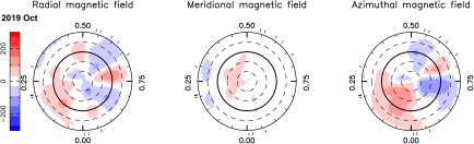
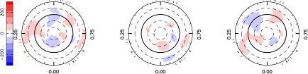
Figure 15: Maps reconstructed with ZDI from SPIRou data collected in 2019 Oct (top) and 2019 Nov-Dec (bottom). See Fig. 3 for a detailed description. These maps are less reliable than those of Fig. 3 due to a SNR of the Stokes $V$ LSD profiles about twice smaller blackthan in the other observing epochs.

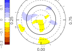
(a) 2019 Oct

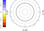
(b) 2019 Nov-Dec

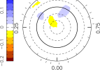
(c) 2020 Aug-Sep

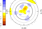
(d) 2020 Sep-Oct

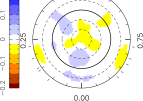
(e) 2020 Dec - 2021 Jan

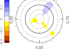
(f) 2021 Oct

Figure 16: blackLogarithmic relative surface brightness maps reconstructed with ZDI for each of the 10 subsets. Yellow regions depict dark cool spots while the bright plages are shown in blue.

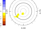
(a) 2021 Nov-Dec

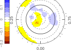
(b) 2022 Jan

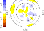
(c) 2022 Nov

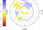
(d) 2023 Jan

Figure 17: blackContinued.

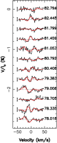
(a) 2019 Oct

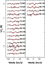
(b) 2019 Nov - Dec

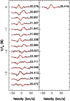
(c) 2020 Aug - Sep

Figure 18: Stokes $V$ LSD profiles associated with the spectra collected between 2019 and 2023. The observed data are in black while the reconstructed profiles derived with ZDI are shown in red. On the right of each profile, we show the rotation cycles while on their left we depict the $3\sigma$ error bar.

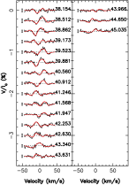
(a) 2020 Sep - Oct

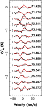
(b) 2020 Dec - 2021 Jan

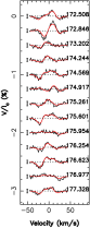
(c) 2021 Oct

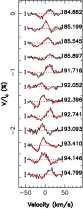
(d) 2021 Nov - Dec

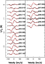
(e) 2022 Jan

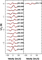
(f) 2022 Nov

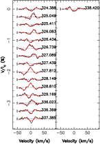
(g) 2023 Jan

Figure 19: Continued.

Appendix C TIMeS reconstruction

We show the magnetic maps reconstructed with TIMeS in Figs. 20 to 24 and the Stokes $V$ LSD profiles fitted with this method in Fig. 25.In Fig. 26, we show the temporal evolution of each of the coefficients describing the magnetic topology found with the TIMeS method.

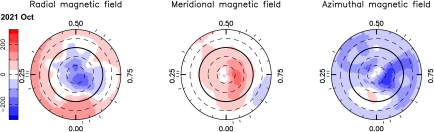
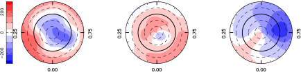
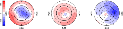
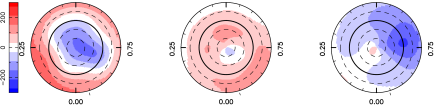
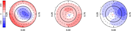
Figure 20: Magnetic maps in 2021 Oct reconstructed with ZDI without differential rotation (first row) and TIMeS (second to fifth rows). We show the TIMeS maps at four specific epochs, that are indicated on the left. See Fig. 3 for a detailed description of the Figure.

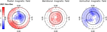
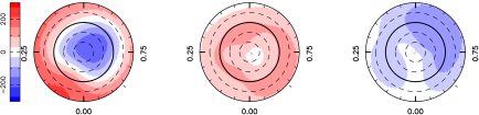
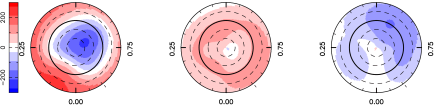
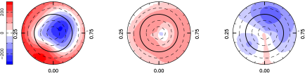
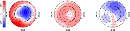
Figure 21: Same as Fig. 20 for 2021 Nov-Dec.

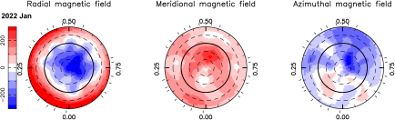
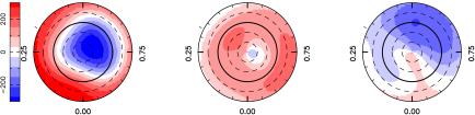
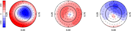
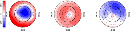
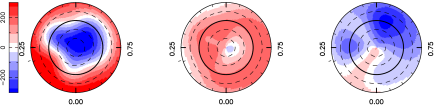
Figure 22: Same as Fig. 20 for 20212 Jan.

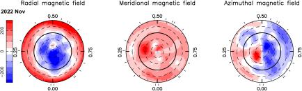
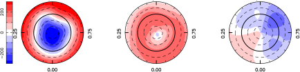
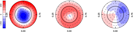
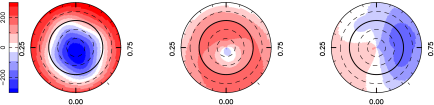
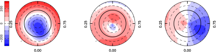
Figure 23: Same as Fig. 20 for 2022 Nov.

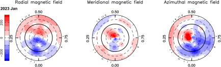
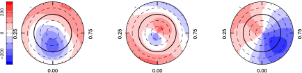
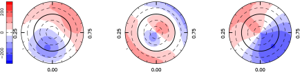
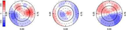
Figure 24: Same as Fig. 20 for 2023 Jan.

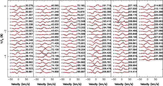
Figure 25: Stokes $V$ LSD profiles used in the TIMeS reconstruction. The observed data are shown in black while the synthetic model is shown in red. The $\chi^{2}_{r}$ between both sets of profiles reaches $1.45$.

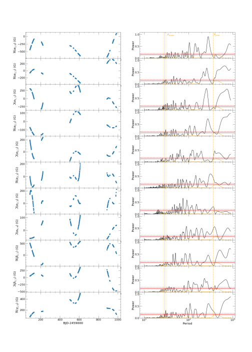
Figure 26: Reconstructed coefficients with TIMeS using Stokes $V$ LSD profiles between 2020 and 2023. Left column: temporal evolution of the 10 coefficients describing the reconstructed magnetic topology, with $\alpha_{\ell,m}$ and $\beta_{\ell,m}$ characterizing the poloidal component and $\gamma_{\ell,m}$ representing the toroidal component ($\ell$ and $m$ being the degree and order of the associated spherical harmonic mode in the expansion). Right column: Periodograms associated with the time series of the reconstructed coefficients, computed using the astropy python. The dotted, dashed and solid red lines show the FAP levels associated with a probability of 1, 0.1 and 0.01%, respectively. blackThe orange curve depicts the window function, the orange solid and dotted vertical lines correspond to the synodic period of the Moon and its 1-yr aliases, respectively, and the orange dashed vertical line outlines the 1-yr period.

Appendix D MCMC results

blackIn Figs. 27, 28, 29, 30 and 31, we show the corner plots of the posterior distributions when using a uniform prior on the orbital period of planet e, and when using a narrow prior on this parameter, centered at $42.9$ d, $46.1$ d, $53.5$ d or $60.5$ d, respectively, assuming circular orbits for all the four planets of the system.

We also list the less likely results provided by the MCMC approach when using the orbital periods derived by Feinstein et al. (2022) in Tables 10 and 11.

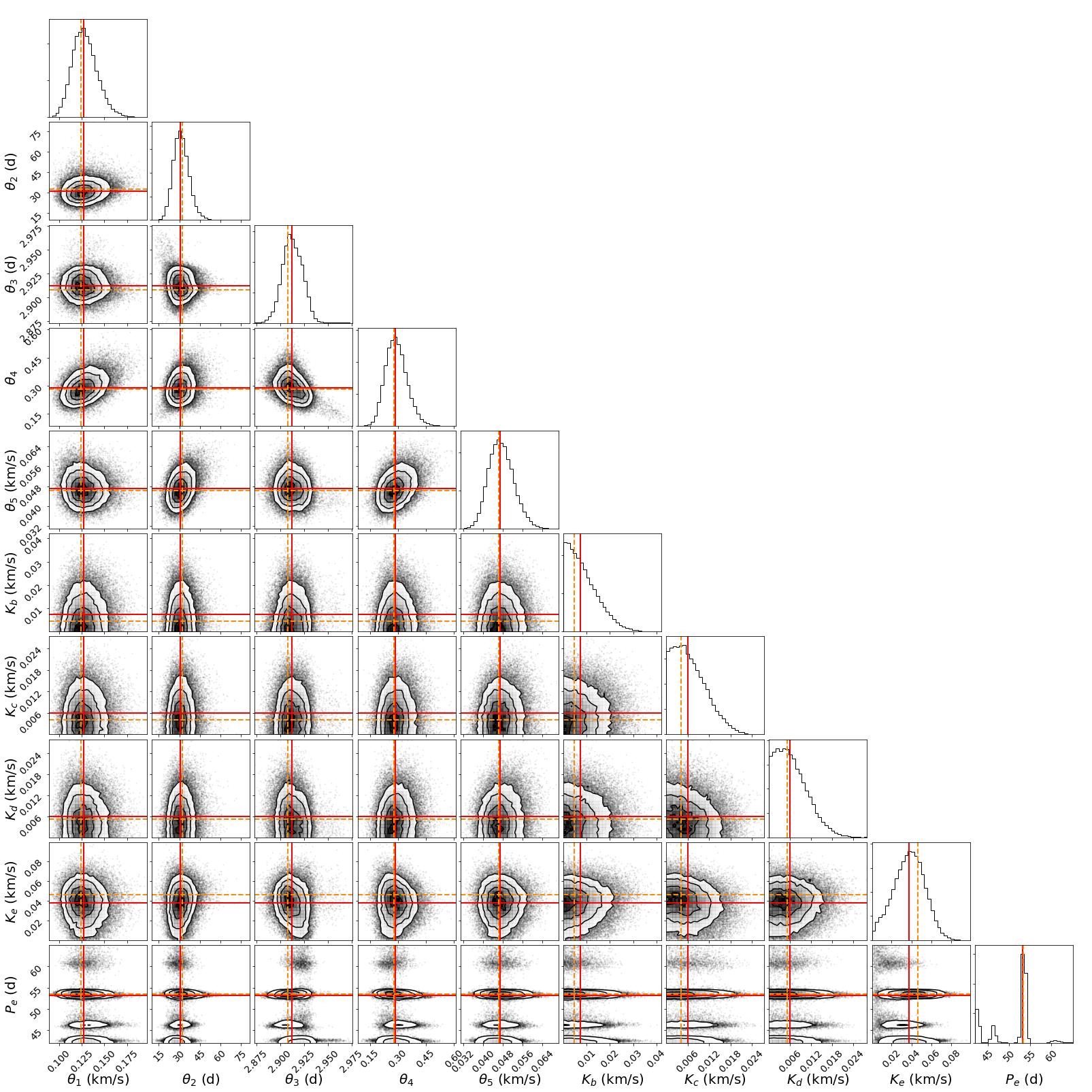
Figure 27: blackCorner plot of the posterior distributions of the hyperparameters of quasi-periodic GP and the planet parameters obtained through a MCMC approach assuming a uniform prior between 42 and 65 d for $P_{e}$. The red lines show the medians of the posterior distributions, while the orange dashed lines correspond to the value that maximizes the log likelihood function, chosen as the optimal parameter. This plot was created using the corner python module (Foreman-Mackey, 2016).

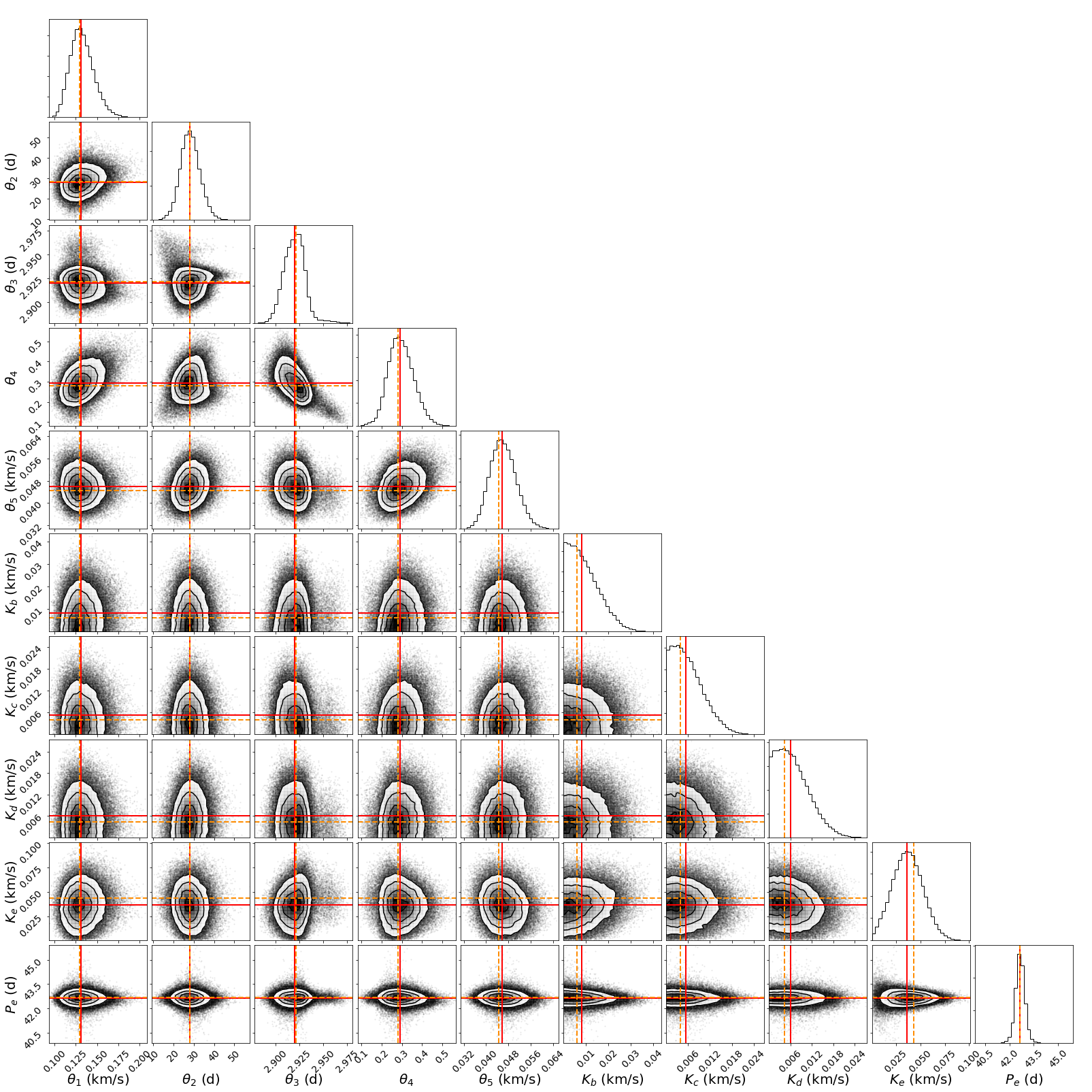
Figure 28: blackSame as Fig. 27 with a narrow prior centered on 42.7 d for $P_{e}$.

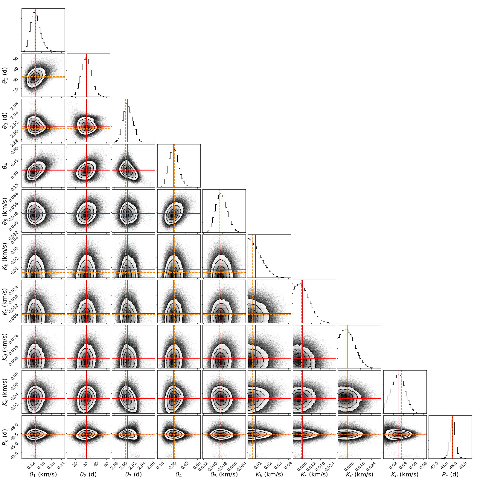
Figure 29: blackSame as Fig. 27 with a narrow prior centered on 46.4 d for $P_{e}$.

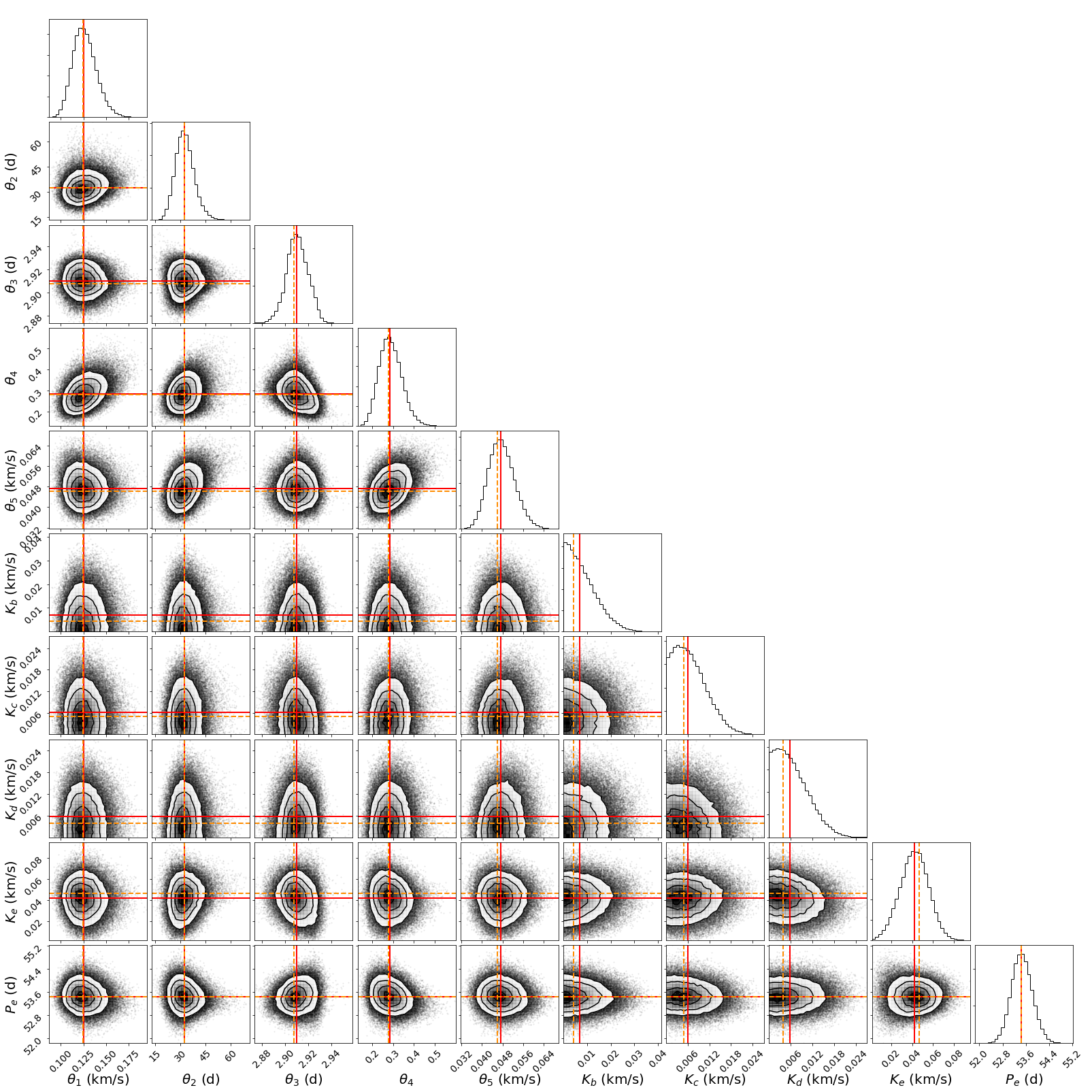
Figure 30: blackSame as Fig. 27 with a narrow prior centered on 53.5 d for $P_{e}$.

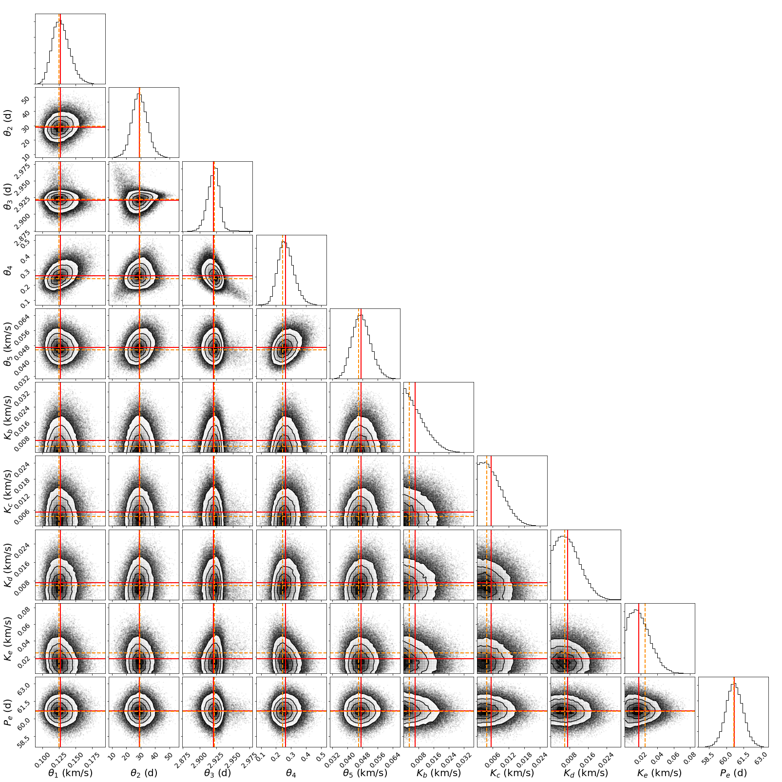
Figure 31: blackSame as Fig. 27 with a narrow prior centered on 60.6 d for $P_{e}$.

Table 10: blackMCMC results for the analysis of the RV data for the 6 planet e orbital periods derived by Feinstein et al. (2022) identified as plausible from our data. 1^st and 2^nd columns list the parameters and their associated priors corresponding to a model featuring an activity signal and four planet-related RV signatures. The 6 last columns show the best value for each parameter, in the case of a narrow prior centred on different values of $P_{e_{0}}$ for the orbital period of planet e. blackThe knee of the modified Jeffreys priors is set to the typical RV uncertainty, noted $\sigma_{RV}$. The log BF is computed with respect to the marginal logarithmic likelihood associated with $P_{e_{0}}=53.0039$ d (see Table 5).

Parameter	Prior	$P_{e_{0}}=61.1583$ d	$P_{e_{0}}=59.6294$ d	$P_{e_{0}}=47.7035$ d	$P_{e_{0}}=62.7678$ d	$P_{e_{0}}=45.0033$ d	$P_{e_{0}}=48.6770$ d
$\theta_{1}$ ($\mathrm{km}\,\mathrm{s}^{-1}$)	mod Jeffreys ($\sigma_{RV}$)	black$0.13\pm 0.01$	black$0.13\pm 0.01$	black$0.13\pm 0.01$	black$0.13\pm 0.01$	black$0.13\pm 0.01$	black$0.13\pm 0.01$
$\theta_{2}$ (d)	log Gaussian ($\log 30$, $\log 2$)	black$30^{+6}_{-5}$	black$30^{+6}_{-5}$	black$29^{+5}_{-4}$	black$30^{+6}_{-5}$	black$30^{+6}_{-5}$	black$30^{+6}_{-5}$
$\theta_{3}$ (d)	Gaussian (2.91, 0.1)	black$2.922\pm 0.008$	black$2.924\pm 0.008$	black$2.918\pm 0.009$	black$2.922\pm 0.009$	black$2.923\pm 0.009$	black$2.925\pm 0.009$
$\theta_{4}$	Uniform (0, 3)	black$0.25\pm 0.05$	black$0.25\pm 0.04$	black$0.27\pm 0.05$	black$0.26\pm 0.05$	black$0.26\pm 0.06$	black$0.25\pm 0.05$
$\theta_{5}$ ($\mathrm{m}\,\mathrm{s}^{-1}$)	mod Jeffreys ($\sigma_{RV}$)	black$46\pm 5$	black$46\pm 5$	black$46\pm 5$	black$46\pm 5$	black$47\pm 5$	black$45\pm 5$
$K_{b}$ ($\mathrm{m}\,\mathrm{s}^{-1}$)	mod Jeffreys ($\sigma_{RV}$)	black$2.9\pm 11.9$	black$3.8\pm 11.2$	black$4.8\pm 10.8$	black$3.5\pm 11.0$	black$3.5\pm 10.6$	black$4.4\pm 10.6$
$P_{b}$ (d)	Fixed from Feinstein et al. (2022)	24.1315	24.1315	24.1315	24.1315	24.1315	24.1315
$T_{b}$ (2459000+)	Fixed from Feinstein et al. (2022)	481.0902	481.0902	481.0902	481.0902	481.0902	481.0902
$R_{b}$ (R♃)	Fixed from Feinstein et al. (2022)	0.85	0.85	0.85	0.85	0.85	0.85
$M_{b}$ (M♃)	Derived from $K_{b}$, $P_{b}$ and $M_{*}$	black$0.05\pm 0.20$	black$0.06\pm 0.19$	black$0.08\pm 0.18$	black$0.06\pm 0.18$	black$0.06\pm 0.18$	black$0.07\pm 0.18$
$\rho_{b}$ ($\rm g\,cm^{-3}$)	Derived from $M_{b}$ and $R_{b}$	black$0.09\pm 0.40$	black$0.13\pm 0.38$	black$0.16\pm 0.36$	black$0.12\pm 0.37$	black$0.12\pm 0.36$	black$0.15\pm 0.36$
$K_{c}$ ($\mathrm{m}\,\mathrm{s}^{-1}$)	mod Jeffreys ($\sigma_{RV}$)	black$3.4\pm 6.5$	black$3.2\pm 6.3$	black$4.2\pm 6.5$	black$3.5\pm 6.5$	black$3.6\pm 6.4$	black$3.3\pm 6.5$
$P_{c}$ (d)	Fixed from Feinstein et al. (2022)	8.2438	8.2438	8.2438	8.2438	8.2438	8.2438
$T_{c}$ (2459000+)	Fixed from Feinstein et al. (2022)	481.1664	481.1664	481.1664	481.1664	481.1664	481.1664
$R_{c}$ (R♃)	Fixed from Feinstein et al. (2022)	0.45	0.45	0.45	0.45	0.45	0.45
$M_{c}$ (M♃)	Derived from $K_{c}$, $P_{c}$ and $M_{*}$	black$0.04\pm 0.07$	black$0.04\pm 0.07$	black$0.05\pm 0.07$	black$0.04\pm 0.07$	black$0.04\pm 0.07$	black$0.04\pm 0.07$
$\rho_{c}$ ($\rm g\,cm^{-3}$)	Derived from $M_{c}$ and $R_{c}$	black$0.55\pm 1.03$	black$0.50\pm 1.00$	black$0.65\pm 1.03$	black$0.56\pm 1.03$	black$0.57\pm 1.01$	black$0.51\pm 1.02$
$K_{d}$ ($\mathrm{m}\,\mathrm{s}^{-1}$)	mod Jeffreys ($\sigma_{RV}$)	black$6.1\pm 6.9$	black$6.4\pm 6.7$	black$5.8\pm 6.8$	black$5.9\pm 6.7$	black$6.8\pm 7.0$	black$5.6\pm 6.6$
$P_{d}$ (d)	Fixed from Feinstein et al. (2022)	12.3960	12.3960	12.3960	12.3960	12.3960	12.3960
$T_{d}$ (2459000+)	Fixed from Feinstein et al. (2022)	478.4149	478.4149	478.4149	478.4149	478.4149	478.4149
$R_{d}$ (R♃)	Fixed from Feinstein et al. (2022)	0.55	0.55	0.55	0.55	0.55	0.55
$M_{d}$ (M♃)	Derived from $K_{d}$, $P_{d}$ and $M_{*}$	black$0.08\pm 0.09$	black$0.08\pm 0.09$	black$0.07\pm 0.09$	black$0.07\pm 0.08$	black$0.09\pm 0.09$	black$0.07\pm 0.08$
$\rho_{d}$ ($\rm g\,cm^{-3}$)	Derived from $M_{d}$ and $R_{d}$	black$0.60\pm 0.68$	black$0.63\pm 0.67$	black$0.58\pm 0.68$	black$0.58\pm 0.67$	black$0.67\pm 0.69$	black$0.56\pm 0.66$
$K_{e}$ ($\mathrm{m}\,\mathrm{s}^{-1}$)	mod Jeffreys ($\sigma_{RV}$)	black$24^{+21}_{-11}$	black$21^{+24}_{-11}$	black$17^{+17}_{-8.6}$	black$15^{+20}_{-8.7}$	black$14^{+17}_{-7.8}$	black$16^{+22}_{-9.3}$
$P_{e}$ (d)	Gaussian ($P_{e_{0}}$, 0.0001)	$61.1583\pm 0.0001$	$59.6294\pm 0.0001$	$47.7035\pm 0.0001$	$62.7678\pm 0.0001$	$45.0033\pm 0.0001$	$48.6770\pm 0.0001$
$T_{e}$ (2459000+)	Fixed from Feinstein et al. (2022)	481.7967	481.7967	481.7967	481.7967	481.7967	481.7967
$R_{e}$ (R♃)	Fixed from Feinstein et al. (2022)	0.89	0.89	0.89	0.89	0.89	0.89
$M_{e}$ (M♃)	Derived from $K_{e}$, $P_{e}$ and $M_{*}$	black$0.55^{+0.47}_{-0.25}$	black$0.47^{+0.55}_{-0.25}$	black$0.36^{+0.36}_{-0.18}$	black$0.35^{+0.45}_{-0.20}$	black$0.29^{+0.36}_{-0.16}$	black$0.34^{+0.45}_{-0.20}$
$\rho_{e}$ ($\rm g\,cm^{-3}$)	Derived from $M_{e}$ and $R_{e}$	black$0.96^{+0.85}_{-0.46}$	black$0.83^{+0.96}_{-0.45}$	black$0.63^{+0.64}_{-0.33}$	black$0.61^{+0.81}_{-0.36}$	black$0.51^{+0.63}_{-0.29}$	black$0.60^{+0.80}_{-0.36}$
$\chi^{2}_{r}$		black5.77	black5.77	black5.64	black5.80	black5.98	black5.63
RMS ($\mathrm{m}\,\mathrm{s}^{-1}$)		black34.4	black34.5	black34.0	black34.4	black35.0	black34.0
$\log\mathcal{L_{M}}$		black$-219.6$	black$-220.3$	black$-220.7$	black$-220.9$	black$-221.0$	black$-221.0$
log BF		black$-3.4$	black$-3.4$	black$-4.5$	black$-4.7$	black$-4.8$	black$-4.8$

Table 11: blackMCMC results for the analysis of the RV data for the 7 planet e orbital periods derived by Feinstein et al. (2022) considered as the less likely ones from our data. 1^st and 2^nd columns list the parameters and their associated priors corresponding to a model featuring an activity signal and four planet-related RV signatures. The 7 last columns show the best value for each parameter, in the case of a narrow prior centred on different values of $P_{e_{0}}$ for the orbital period of planet e. blackThe knee of the modified Jeffreys priors is set to the typical RV uncertainty, noted $\sigma_{RV}$. The log BF is computed with respect to the marginal logarithmic likelihood associated with $P_{e_{0}}=53.0039$ d (see Table 5).

Parameter	Prior	$P_{e_{0}}=51.8516$ d	$P_{e_{0}}=44.1699$ d	$P_{e_{0}}=49.6911$ d	$P_{e_{0}}=55.4692$ d	$P_{e_{0}}=50.7484$ d	$P_{e_{0}}=58.1750$ d	$P_{e_{0}}=56.7899$ d
$\theta_{1}$ ($\mathrm{km}\,\mathrm{s}^{-1}$)	mod Jeffreys ($\sigma_{RV}$)	black$0.13\pm 0.01$	black$0.13\pm 0.01$	black$0.13\pm 0.01$	black$0.13\pm 0.01$	black$0.13\pm 0.01$	black$0.13\pm 0.01$	black$0.13\pm 0.01$
$\theta_{2}$ (d)	log Gaussian ($\log 30$, $\log 2$)	black$30^{+6}_{-5}$	black$29^{+6}_{-5}$	black$29^{+6}_{-5}$	black$30^{+6}_{-5}$	black$29^{+6}_{-5}$	black$30^{+6}_{-5}$	black$30^{+6}_{-5}$
$\theta_{3}$ (d)	Gaussian (2.91, 0.1)	black$2.922\pm 0.009$	black$2.922\pm 0.009$	black$2.923\pm 0.009$	black$2.924\pm 0.008$	black$2.923\pm 0.009$	black$2.924\pm 0.008$	black$2.924\pm 0.008$
$\theta_{4}$	Uniform (0, 3)	black$0.26\pm 0.06$	black$0.26\pm 0.05$	black$0.25\pm 0.05$	black$0.25\pm 0.05$	black$0.25\pm 0.05$	black$0.25\pm 0.05$	black$0.25\pm 0.05$
$\theta_{5}$ ($\mathrm{m}\,\mathrm{s}^{-1}$)	mod Jeffreys ($\sigma_{RV}$)	black$46\pm 5$	black$46\pm 5$	black$46\pm 5$	black$46\pm 5$	black$46\pm 5$	black$46\pm 5$	black$46\pm 5$
$K_{b}$ ($\mathrm{m}\,\mathrm{s}^{-1}$)	mod Jeffreys ($\sigma_{RV}$)	black$3.6\pm 10.9$	black$3.5\pm 11.3$	black$3.8\pm 10.2$	black$3.7\pm 10.9$	black$3.6\pm 11.4$	black$3.7\pm 11.3$	black$3.7\pm 11.1$
$P_{b}$ (d)	Fixed from Feinstein et al. (2022)	24.1315	24.1315	24.1315	24.1315	24.1315	24.1315	24.1315
$T_{b}$ (2459000+)	Fixed from Feinstein et al. (2022)	481.0902	481.0902	481.0902	481.0902	481.0902	481.0902	481.0902
$R_{b}$ (R♃)	Fixed from Feinstein et al. (2022)	0.85	0.85	0.85	0.85	0.85	0.85	0.85
$M_{b}$ (M♃)	Derived from $K_{b}$, $P_{b}$ and $M_{*}$	black$0.06\pm 0.18$	black$0.05\pm 0.19$	black$0.06\pm 0.17$	black$0.06\pm 0.18$	black$0.06\pm 0.19$	black$0.06\pm 0.19$	black$0.06\pm 0.19$
$\rho_{b}$ ($\rm g\,cm^{-3}$)	Derived from $M_{b}$ and $R_{b}$	black$0.12\pm 0.37$	black$0.12\pm 0.38$	black$0.13\pm 0.35$	black$0.13\pm 0.37$	black$0.12\pm 0.39$	black$0.13\pm 0.38$	black$0.13\pm 0.37$
$K_{c}$ ($\mathrm{m}\,\mathrm{s}^{-1}$)	mod Jeffreys ($\sigma_{RV}$)	black$4.0\pm 6.5$	black$3.4\pm 6.4$	black$3.1\pm 6.2$	black$3.5\pm 6.5$	black$3.7\pm 6.5$	black$3.4\pm 6.1$	black$3.6\pm 6.2$
$P_{c}$ (d)	Fixed from Feinstein et al. (2022)	8.2438	8.2438	8.2438	8.2438	8.2438	8.2438	8.2438
$T_{c}$ (2459000+)	Fixed from Feinstein et al. (2022)	481.1664	481.1664	481.1664	481.1664	481.1664	481.1664	481.1664
$R_{c}$ (R♃)	Fixed from Feinstein et al. (2022)	0.45	0.45	0.45	0.45	0.45	0.45	0.45
$M_{c}$ (M♃)	Derived from $K_{c}$, $P_{c}$ and $M_{*}$	black$0.04\pm 0.07$	black$0.04\pm 0.07$	black$0.03\pm 0.07$	black$0.04\pm 0.07$	black$0.04\pm 0.07$	black$0.04\pm 0.07$	black$0.04\pm 0.07$
$\rho_{c}$ ($\rm g\,cm^{-3}$)	Derived from $M_{c}$ and $R_{c}$	black$0.63\pm 1.03$	black$0.54\pm 1.02$	black$0.49\pm 0.98$	black$0.56\pm 1.02$	black$0.59\pm 1.03$	black$0.55\pm 0.97$	black$0.56\pm 0.98$
$K_{d}$ ($\mathrm{m}\,\mathrm{s}^{-1}$)	mod Jeffreys ($\sigma_{RV}$)	black$6.0\pm 6.8$	black$7.0\pm 6.4$	black$6.3\pm 6.7$	black$6.1\pm 6.7$	black$6.3\pm 6.7$	black$6.5\pm 6.4$	black$5.9\pm 6.8$
$P_{d}$ (d)	Fixed from Feinstein et al. (2022)	12.3960	12.3960	12.3960	12.3960	12.3960	12.3960	12.3960
$T_{d}$ (2459000+)	Fixed from Feinstein et al. (2022)	478.4149	478.4149	478.4149	478.4149	478.4149	478.4149	478.4149
$R_{d}$ (R♃)	Fixed from Feinstein et al. (2022)	0.55	0.55	0.55	0.55	0.55	0.55	0.55
$M_{d}$ (M♃)	Derived from $K_{d}$, $P_{d}$ and $M_{*}$	black$0.08\pm 0.09$	black$0.09\pm 0.08$	black$0.08\pm 0.08$	black$0.08\pm 0.08$	black$0.08\pm 0.08$	black$0.08\pm 0.08$	black$0.08\pm 0.09$
$\rho_{d}$ ($\rm g\,cm^{-3}$)	Derived from $M_{d}$ and $R_{d}$	black$0.60\pm 0.68$	black$0.69\pm 0.65$	black$0.63\pm 0.66$	black$0.60\pm 0.67$	black$0.63\pm 0.67$	black$0.64\pm 0.64$	black$0.59\pm 0.68$
$K_{e}$ ($\mathrm{m}\,\mathrm{s}^{-1}$)	mod Jeffreys ($\sigma_{RV}$)	black$12^{+17}_{-7.2}$	black$9.5^{+14.4}_{-5.7}$	black$8.6^{+13.7}_{-5.3}$	black$8.6^{+15.0}_{-5.5}$	black$6.5^{+11.0}_{-4.1}$	black$6.8^{+11.8}_{-4.3}$	black$4.0^{+7.4}_{-2.6}$
$P_{e}$ (d)	Gaussian ($P_{e_{0}}$, 0.0001)	$51.8516\pm 0.0001$	$44.1699\pm 0.0001$	$49.6911\pm 0.0001$	$55.4692\pm 0.0001$	$50.7484\pm 0.0001$	$58.1750\pm 0.0001$	$56.7899\pm 0.0001$
$T_{e}$ (2459000+)	Fixed from Feinstein et al. (2022)	481.7967	481.7967	481.7967	481.7967	481.7967	481.7967	481.7967
$R_{e}$ (R♃)	Fixed from Feinstein et al. (2022)	0.89	0.89	0.89	0.89	0.89	0.89	0.89
$M_{e}$ (M♃)	Derived from $K_{e}$, $P_{e}$ and $M_{*}$	black$0.26^{+0.38}_{-0.16}$	black$0.19^{+0.29}_{-0.12}$	black$0.18^{+0.28}_{-0.12}$	black$0.19^{+0.33}_{-0.12}$	black$0.14^{+0.23}_{-0.08}$	black$0.15^{+0.26}_{-0.09}$	black$0.08^{+0.17}_{-0.05}$
$\rho_{e}$ ($\rm g\,cm^{-3}$)	Derived from $M_{e}$ and $R_{e}$	black$0.46^{+0.66}_{-0.27}$	black$0.34^{+0.51}_{-0.21}$	black$0.32^{+0.50}_{-0.20}$	black$0.34^{+0.58}_{-0.22}$	black$0.24^{+0.41}_{-0.16}$	black$0.26^{+0.46}_{-0.17}$	black$0.16^{+0.28}_{-0.11}$
$\chi^{2}_{r}$		black5.81	black5.73	black5.65	black5.73	black5.70	black5.73	black5.71
RMS ($\mathrm{m}\,\mathrm{s}^{-1}$)		black34.5	black34.3	black34.0	black34.3	black34.2	black34.3	black34.2
$\log\mathcal{L_{M}}$		black$-221.3$	black$-221.6$	black$-221.6$	black$-221.8$	black$-222.1$	black$-222.1$	black$-222.6$
log BF		black$-5.1$	black$-5.4$	black$-5.4$	black$-5.6$	black$-5.9$	black$-5.9$	black$-6.4$

References

- Artigau et al. (2014) Artigau É., et al., 2014, in Peck A. B., Benn C. R., Seaman R. L., eds, Society of Photo-Optical Instrumentation Engineers (SPIE) Conference Series Vol. 9149, Observatory Operations: Strategies, Processes, and Systems V. p. 914905 (arXiv:1406.6927), doi:10.1117/12.2056385
- Artigau et al. (2022) Artigau É., et al., 2022, AJ, 164, 84
- Ataiee et al. (2018) Ataiee S., Baruteau C., Alibert Y., Benz W., 2018, A&A, 615, A110
- Baraffe et al. (2008) Baraffe I., Chabrier G., Barman T., 2008, A&A, 482, 315
- Baraffe et al. (2015) Baraffe I., Homeier D., Allard F., Chabrier G., 2015, A&A, 577, A42
- Baruteau & Papaloizou (2013) Baruteau C., Papaloizou J. C. B., 2013, ApJ, 778, 7
- Baruteau et al. (2014) Baruteau C., et al., 2014, in Beuther H., Klessen R. S., Dullemond C. P., Henning T., eds, Protostars and Planets VI. p. 667 (arXiv:1312.4293), doi:10.2458/azu_uapress_9780816531240-ch029
- Batygin & Morbidelli (2013) Batygin K., Morbidelli A., 2013, AJ, 145, 1
- Binkert et al. (2021) Binkert F., Szulágyi J., Birnstiel T., 2021, MNRAS, 506, 5969
- Blunt et al. (2023) Blunt S., et al., 2023, AJ, 166, 62
- Booth & Ilee (2019) Booth R. A., Ilee J. D., 2019, MNRAS, 487, 3998
- Brown et al. (1991) Brown S. F., Donati J. F., Rees D. E., Semel M., 1991, A&A, 250, 463
- Chametla et al. (2022) Chametla R. O., Masset F. S., Baruteau C., Bitsch B., 2022, MNRAS, 510, 3867
- Chib & Jeliazkov (2001) Chib S., Jeliazkov I., 2001, Journal of the American Statistical Association, 96, 270
- Claret & Bloemen (2011) Claret A., Bloemen S., 2011, A&A, 529, A75
- Cook et al. (2022) Cook N. J., et al., 2022, PASP, 134, 114509
- David et al. (2016) David T. J., et al., 2016, Nature, 534, 658
- David et al. (2019a) David T. J., et al., 2019a, ApJ, 158, 79
- David et al. (2019b) David T. J., Petigura E. A., Luger R., Foreman-Mackey D., Livingston J. H., Mamajek E. E., Hillenbrand L. A., 2019b, ApJ, 885, L12
- Donati & Brown (1997) Donati J. F., Brown S. F., 1997, A&A, 326, 1135
- Donati et al. (1997) Donati J.-F., Semel M., Carter B. D., Rees D. E., Collier Cameron A., 1997, MNRAS, 291, 658
- Donati et al. (2000) Donati J. F., Mengel M., Carter B. D., Marsden S., Collier Cameron A., Wichmann R., 2000, MNRAS, 316, 699
- Donati et al. (2003a) Donati J. F., et al., 2003a, MNRAS, 345, 1145
- Donati et al. (2003b) Donati J. F., Collier Cameron A., Petit P., 2003b, MNRAS, 345, 1187
- Donati et al. (2006) Donati J. F., et al., 2006, MNRAS, 370, 629
- Donati et al. (2016) Donati J. F., et al., 2016, Nature, 534, 662
- Donati et al. (2020) Donati J. F., et al., 2020, MNRAS, 491, 5660
- Donati et al. (2023) Donati J. F., et al., 2023, MNRAS, 525, 455
- Feinstein et al. (2021) Feinstein A. D., Montet B. T., Johnson M. C., Bean J. L., David T. J., Gully-Santiago M. A., Livingston J. H., Luger R., 2021, AJ, 162, 213
- Feinstein et al. (2022) Feinstein A. D., David T. J., Montet B. T., Foreman-Mackey D., Livingston J. H., Mann A. W., 2022, ApJ, 925, L2
- Finociety & Donati (2022) Finociety B., Donati J.-F., 2022, Monthly Notices of the Royal Astronomical Society, 516, 5887
- Finociety et al. (2021) Finociety B., et al., 2021, MNRAS, 508, 3427
- Finociety et al. (2023) Finociety B., et al., 2023, MNRAS, 520, 3049
- Foreman-Mackey (2016) Foreman-Mackey D., 2016, The Journal of Open Source Software, 1, 24
- Foreman-Mackey et al. (2013) Foreman-Mackey D., Hogg D. W., Lang D., Goodman J., 2013, PASP, 125, 306
- Fortney et al. (2007) Fortney J. J., Marley M. S., Barnes J. W., 2007, ApJ, 659, 1661
- Gaia Collaboration et al. (2023) Gaia Collaboration et al., 2023, A&A, 674, A1
- Gaidos et al. (2022) Gaidos E., et al., 2022, MNRAS, 509, 2969
- Goldberg et al. (2022) Goldberg M., Batygin K., Morbidelli A., 2022, Icarus, 388, 115206
- Grankin (2013) Grankin K. N., 2013, Astronomy Letters, 39, 251
- Jeffers et al. (2007) Jeffers S. V., Donati J. F., Collier Cameron A., 2007, MNRAS, 375, 567
- Kővári et al. (2004) Kővári Z., Strassmeier K. G., Granzer T., Weber M., Oláh K., Rice J. B., 2004, A&A, 417, 1047
- Krolikowski et al. (2021) Krolikowski D. M., Kraus A. L., Rizzuto A. C., 2021, AJ, 162, 110
- Landi Degl’Innocenti & Landolfi (2004) Landi Degl’Innocenti E., Landolfi M., 2004, Polarisation in Spectral Lines. Kluwer Academic Publishers, Dordrecht
- Lehtinen et al. (2022) Lehtinen J. J., et al., 2022, A&A, 660, A141
- Loeillet et al. (2008) Loeillet B., et al., 2008, A&A, 481, 529
- Maggio et al. (2022) Maggio A., et al., 2022, ApJ, 925, 172
- Mann et al. (2016) Mann A. W., et al., 2016, AJ, 152, 61
- Martioli et al. (2021) Martioli E., Hébrard G., Correia A. C. M., Laskar J., Lecavelier des Etangs A., 2021, A&A, 649, A177
- Ment et al. (2018) Ment K., Fischer D. A., Bakos G., Howard A. W., Isaacson H., 2018, AJ, 156, 213
- Paardekooper et al. (2013) Paardekooper S.-J., Rein H., Kley W., 2013, MNRAS, 434, 3018
- Pacetti et al. (2022) Pacetti E., et al., 2022, ApJ, 937, 36
- Petit et al. (2002) Petit P., Donati J. F., Collier Cameron A., 2002, MNRAS, 334, 374
- Pierens et al. (2011) Pierens A., Baruteau C., Hersant F., 2011, A&A, 531, A5
- Plavchan et al. (2020) Plavchan P., et al., 2020, Nature, 582, 497
- Poljančić Beljan et al. (2022) Poljančić Beljan I., et al., 2022, A&A, 663, A24
- Poppenhaeger et al. (2021) Poppenhaeger K., Ketzer L., Mallonn M., 2021, MNRAS, 500, 4560
- Rajpaul et al. (2015) Rajpaul V., Aigrain S., Osborne M. A., Reece S., Roberts S., 2015, MNRAS, 452, 2269
- Rasmussen & Williams (2006) Rasmussen C., Williams C., 2006, Gaussian Processes for Machine Learning. Adaptive Computation and Machine Learning, MIT Press, Cambridge, MA, USA
- Rincon (2019) Rincon F., 2019, Journal of Plasma Physics, 85, 205850401
- Rizzuto et al. (2020) Rizzuto A. C., et al., 2020, AJ, 160, 33
- Ryabchikova et al. (2015) Ryabchikova T., Piskunov N., Kurucz R. L., Stempels H. C., Heiter U., Pakhomov Y., Barklem P. S., 2015, Phys. Scr., 90, 054005
- Schneider & Bitsch (2021) Schneider A. D., Bitsch B., 2021, A&A, 654, A71
- Semel (1989) Semel M., 1989, A&A, 225, 456
- Short & Doyle (1998) Short C. I., Doyle J. G., 1998, A&A, 331, L5
- Siess et al. (2000) Siess L., Dufour E., Forestini M., 2000, A&A, 358, 593
- Sikora et al. (2023) Sikora J., et al., 2023, arXiv e-prints, p. arXiv:2304.00797
- Strugarek et al. (2015) Strugarek A., Brun A. S., Matt S. P., Réville V., 2015, ApJ, 815, 111
- Suárez Mascareño et al. (2021) Suárez Mascareño A., et al., 2021, Nature Astronomy, 6, 232
- Szabó et al. (2022) Szabó G. M., et al., 2022, A&A, 659, L7
- Szulágyi et al. (2022) Szulágyi J., Binkert F., Surville C., 2022, ApJ, 924, 1
- Tejada Arevalo et al. (2022) Tejada Arevalo R., Tamayo D., Cranmer M., 2022, ApJ, 932, L12
- Thorngren et al. (2016) Thorngren D. P., Fortney J. J., Murray-Clay R. A., Lopez E. D., 2016, ApJ, 831, 64
- Turrini et al. (2021) Turrini D., et al., 2021, ApJ, 909, 40
- Turrini et al. (2023) Turrini D., et al., 2023, arXiv e-prints, p. arXiv:2307.08653
- Van Eylen et al. (2019) Van Eylen V., et al., 2019, AJ, 157, 61
- Venturini & Helled (2020) Venturini J., Helled R., 2020, A&A, 634, A31
- Vissapragada et al. (2021) Vissapragada S., et al., 2021, AJ, 162, 222
- Yu et al. (2017) Yu L., et al., 2017, MNRAS, 467, 1342
- Yu et al. (2019) Yu L., et al., 2019, MNRAS, 489, 5556
- Zakhozhay et al. (2022) Zakhozhay O. V., et al., 2022, A&A, 667, L14
- Zechmeister & Kürster (2009) Zechmeister M., Kürster M., 2009, A&A, 496, 577
- Zirin (1982) Zirin H., 1982, ApJ, 260, 655