Analyzing and Improving OT-based Adversarial Networks

Abstract

Optimal Transport (OT) problem aims to find a transport plan that bridges two distributions while minimizing a given cost function. OT theory has been widely utilized in generative modeling. In the beginning, OT distance has been used as a measure for assessing the distance between data and generated distributions. Recently, OT transport map between data and prior distributions has been utilized as a generative model. These OT-based generative models share a similar adversarial training objective. In this paper, we begin by unifying these OT-based adversarial methods within a single framework. Then, we elucidate the role of each component in training dynamics through a comprehensive analysis of this unified framework. Moreover, we suggest a simple but novel method that improves the previously best-performing OT-based model. Intuitively, our approach conducts a gradual refinement of the generated distribution, progressively aligning it with the data distribution. Our approach achieves a FID score of 2.51 on CIFAR-10, outperforming unified OT-based adversarial approaches.

1 Introduction

Optimal Transport (OT) theory addresses the most cost-efficient way to transport one probability distribution to another (Villani et al., 2009; Peyré et al., 2017). OT theory has been widely exploited in various machine learning applications, such as generative modeling (Arjovsky et al., 2017; Rout et al., ), domain adaptation (Guan et al., 2021; Shen et al., 2018), unpaired image-to-image translation (Korotin et al., 2022; Xie et al., 2019), point cloud approximation (Mérigot et al., 2021), and data augmentation (Alvarez-Melis & Fusi, 2020; Flamary et al., 2016). In this work, we focus on OT-based generative modeling. During its early stages, WGAN (Arjovsky et al., 2017) and its variants (Gulrajani et al., 2017; Petzka et al., ; Liu et al., 2019; Miyato et al., ) introduced OT theory to define loss functions in GANs (Goodfellow et al., 2020) (OT Loss). More precisely, OT-based Wasserstein distance is introduced for measuring a distance between data and generated distributions. These approaches have shown relative stability and improved performance compared to the vanilla GAN (Gulrajani et al., 2017). However, these models still face challenges, such as an unstable training process and limited expressivity (Sanjabi et al., 2018; Mescheder et al., 2018).

Recently, an alternative approach has been introduced in OT-based generative modeling. These works consider OT problems between noise prior and data distributions, aiming to learn the transport map between them (An et al., 2019; 2020; Fan et al., ; Rout et al., ) (OT Map). This transport map serves as a generative model because it moves a noise sample into a data sample. In this context, two noteworthy methods have been proposed: OTM (Rout et al., ) and UOTM (Choi et al., 2023a). Interestingly, these two algorithms present similar adversarial training algorithms as previous OT Loss approaches, like WGAN, but with additional cost function and composition with convex functions (Eq 5 and 8). These models, especially UOTM, demonstrated promising outcomes, particularly in terms of stability in convergence and performance. Nevertheless, despite the success of OT Map approaches, there is a lack of understanding about why they achieve such high performance and what their limitations are.

(i) In this paper, we propose a unified framework that integrates previous OT Loss and OT Map approaches. Since both of these approaches utilize GAN-like adversarial training, we collectively refer to them as OT-based GANs. (ii) Utilizing this framework, we conduct a comprehensive analysis of previous OT-based GANs for an in-depth analysis of each constituent factor of OT Map. Our analysis reveals that the cost function mitigates the mode collapse problem, and the incorporation of a strictly convex function into discriminator loss is beneficial for the stability of the algorithm. (iii) Moreover, we propose a straightforward but novel method for improving the previous best-performing OT-based GANs, i.e., UOTM. Our method involves a gradual up-weighting of divergence terms in the Unbalanced Optimal Transport problem. In this respect, we refer to our model as UOTM with Scheduled Divergence (UOTM-SD). This gradual up-weighting of divergence terms in UOTM-SD leads to the convergence of the optimal transport plan from the UOT problem toward that of the OT problem. Our UOTM-SD outperforms UOTM and significantly improves the sensitivity of UOTM to the cost-intensity hyperparameter. Our contributions can be summarized as follows:

• We introduce an integrated framework that encompasses previous OT-based GANs.

• We present a comparative analysis of these OT-based GANs to elucidate the role of each component.

• We propose a simple and well-motivated modification to UOTM that improves both generation results and $\tau$-robustness of UOTM for the cost function $c(x,y)=\tau\|x-y\|_{2}^{2}$.

Notations

Let $\mathcal{X}$, $\mathcal{Y}$ be compact Polish spaces and $\mu$ and $\nu$ be probability distributions on $\mathcal{X}$ and $\mathcal{Y}$, respectively. Assume that these probability spaces satisfy some regularity conditions described in Appendix A. We denote the prior (source) distribution as $\mu$ and data (target) distributions as $\nu$. $\mathcal{M}_{+}(\mathcal{X}\times\mathcal{Y})$ represents the set of positive measures on $\mathcal{X}\times\mathcal{Y}$. For $\pi\in\mathcal{M}_{+}(\mathcal{X}\times\mathcal{Y})$, we denote the marginals with respect to $\mathcal{X}$ and $\mathcal{Y}$ as $\pi_{0}$ and $\pi_{1}$. For a measurable map $T:\mathcal{X}\rightarrow\mathcal{Y}$, $T_{\#}\mu$ denotes the associated pushforward distribution of $\mu$. $c(x,y)$ refers to the transport cost function defined on $\mathcal{X}\times\mathcal{Y}$. In this paper, we assume $\mathcal{X},\mathcal{Y}\subset\mathbb{R}^{d}$ and the quadratic cost $c(x,y)=\tau\lVert x-y\rVert_{2}^{2}$, where $\tau$ is a given positive constant. For a detailed explanation of notations and assumptions, see Appendix A.

2 Background and Related Works

In this section, we introduce several OT problems and their equivalent forms. Then, we provide an overview of various OT-based GANs, which will be the subject of our analysis.

Kantorovich OT

Kantorovich (1948) formulated the OT problem through the cost-minimizing coupling $\pi\in\Pi(\mu,\nu)$ between the source distribution $\mu$ and the target distribution $\nu$ as follows:

$$C(\mu,\nu):=\inf_{\pi\in\Pi(\mu,\nu)}\left[\int_{\mathcal{X}\times\mathcal{Y}}c(x,y)d\pi(x,y)\right],$$ (1)

Under mild assumptions, this Kantorovich problem can be reformulated into several equivalent forms, such as the dual (Eq 2) and semi-dual (Eq 3) formulation (Villani et al., 2009):

$$C(\mu,\nu) =\sup_{u(x)+v(y)\leq c(x,y)}\left[\int_{\mathcal{X}}u(x)d\mu(x)+\int_{\mathcal{Y}}v(y)d\nu(y)\right],$$ (2)

$$=\sup_{v\in L^{1}(\nu)}\left[\int_{\mathcal{X}}v^{c}(x)d\mu(x)+\int_{\mathcal{Y}}v(y)d\nu(y)\right],$$ (3)

where $u$ and $v$ are Lebesgue integrable with respect to measure $\mu$ and $\nu$, i.e., $u\in L^{1}(\mu)$ and $v\in L^{1}(\nu)$, and the $c$-transform $v^{c}(x):=\inf_{y\in\mathcal{Y}}\left(c(x,y)-v(y)\right)$. For a particular case where the cost $c(\cdot,\cdot)$ is a distance function, i.e., the Wasserstein-1 distance, then $u=-v$ and $u$ is 1-Lipschitz (Villani et al., 2009). In such case, we call Eq 2 a Kantorovich-Rubinstein duality.

OT Loss in GANs

WGAN (Arjovsky et al., 2017) introduced the Wasserstein-1 distance to define a loss function in GAN. This Wasserstein distance serves as a distance measure between generated distribution and data distribution. From Kantorovich-Rubinstein duality, the learning objective for WGAN is given as follows:

$$\mathcal{L}_{v_{\phi},T_{\theta}}=\sup_{\lVert v_{\phi}\rVert_{L}\leq 1}\inf_{T_{\theta}}\left[-\int_{\mathcal{X}}v_{\phi}\left(T_{\theta}(x)\right)d\mu(x)+\int_{\mathcal{Y}}v_{\phi}(y)d\nu(y)\right],$$ (4)

where the potential (critic) $v_{\phi}$ is 1-Lipschitz, i.e., $\lVert v_{\phi}\rVert_{L}\leq 1$, and $T_{\theta}$ is a generator. WGAN-GP (Gulrajani et al., 2017) suggested a gradient penalty regularizer to enhance the stability of WGAN training. For optimal coupling $\pi^{*}$, the optimal potential $v_{\phi}^{*}$ satisfies $\lVert\nabla v_{\phi}(\hat{y})\rVert_{2}=1$ $\pi^{*}$-almost surely, where $\hat{y}=tT_{\theta}(x)+(1-t)y$ for some $0\leq t\leq 1$ with $\left(T_{\theta}(x),y\right)\sim\pi^{*}$. WGAN-GP exploits this optimality condition by introducing $\mathcal{R}(x,y)=\left(\lVert\nabla v_{\phi}(\hat{y})\rVert_{2}-1\right)^{2}$ as the penalty term.

OT Map as Generative model

Parallel to OT Loss approaches, there has been a surge of research on directly modeling the optimal transport map between the input prior distribution and the real data distribution (Rout et al., ; An et al., 2019; 2020; Makkuva et al., 2020; Yang & Uhler, 2019; Choi et al., 2023a). In this case, the optimal transport map serves as the generator itself. In particular, Rout et al. and Fan et al. leverage the semi-dual formulation (Eq 3) of the Kantorovich problem for generative modeling. Specifically, these models parametrize $v=v_{\phi}$ in Eq 3 and represent its $c$-transform $v^{c}$ through the transport map $T_{\theta}:\mathcal{X}\rightarrow\mathcal{Y},\,\,x\mapsto\arg\inf_{y\in\mathcal{Y}}\left[c(x,y)-v\left(y\right)\right]$. Then, we obtain the following min-max objective:

$$\mathcal{L}_{v_{\phi},T_{\theta}}=\sup_{v_{\phi}}\left[\int_{\mathcal{X}}\inf_{T_{\theta}}\left[c\left(x,T_{\theta}(x)\right)-v_{\phi}\left(T_{\theta}(x)\right)\right]d\mu(x)+\int_{\mathcal{Y}}v_{\phi}(y)d\nu(y)\right].$$ (5)

Intuitively, $T_{\theta}$ and $v_{\phi}$ serve as the generator and the discriminator of a GAN. For convenience, we denote the optimization problem of Eq 5 as an OT-based generative model (OTM) (Fan et al., ). Note that, if we consider $c=0$, this objective has the same form as WGAN (Eq 4) without the Lipschitz constraint.

Recently, Choi et al. (2023a) extended OTM by leveraging the semi-dual form of the Unbalanced Optimal Transport (UOT) problem (Chizat et al., 2018; Liero et al., 2018). UOT extends the classical OT problem by relaxing the strict marginal constraints using the Csiszàr divergences $D_{\Psi_{i}}$. Formally, the UOT problem (Eq 6) and its semi-dual form (Eq 7) are defined as follows:

$$C_{ub}(\mu,\nu) =\inf_{\pi\in\mathcal{M}_{+}(\mathcal{X}\times\mathcal{Y})}\left[\int_{\mathcal{X}\times\mathcal{Y}}c(x,y)d\pi(x,y)+D_{\Psi_{1}}(\pi_{0}|\mu)+D_{\Psi_{2}}(\pi_{1}|\nu)\right],$$ (6)

$$=\sup_{v\in\mathcal{C(Y)}}\left[\int_{\mathcal{X}}-\Psi_{1}^{*}\left(-v^{c}(x))\right)d\mu(x)+\int_{\mathcal{Y}}-\Psi^{*}_{2}(-v(y))d\nu(y)\right],$$ (7)

where $\mathcal{C(Y)}$ denotes a set of continuous functions over $\mathcal{Y}$. Here, the entropy function $\Psi_{i}:\mathbb{R}\rightarrow[0,\infty]$ is a convex, lower semi-continuous, and non-negative function, and $\Psi_{i}(x)=\infty\text{ for }x<0$. $\Psi_{i}^{*}$ denotes its convex conjugate. Note that for non-negative $\Psi_{i}$, $\Psi_{i}^{*}$ is a non-decreasinig convex function. For simplicity, we assume $\Psi_{i}^{*}(0)=0,(\Psi_{i}^{*})^{\prime}(0)=1$. The reason for this assumption will be clarified in Sec 4. By employing the same parametrization as in Eq 5, we arrive at the following optimization problem:

$$\mathcal{L}_{v_{\phi},T_{\theta}}=\inf_{v_{\phi}}\left[\int_{\mathcal{X}}\Psi_{1}^{*}\left(-\inf_{T_{\theta}}\left[c\left(x,T_{\theta}(x)\right)-v_{\phi}\left(T_{\theta}(x)\right)\right]\right)d\mu(x)+\int_{\mathcal{Y}}\Psi^{*}_{2}\left(-v_{\phi}(y)\right)d\nu(y)\right].$$ (8)

We call such an optimization problem a UOT-based generative model (UOTM) (Choi et al., 2023a).

3 Analyzing OT-based Adversarial Approaches

In this section, we suggest a unified framework for OT-based GANs (Sec 3.1). Using this unified framework, we compare the dynamics of each algorithm through various experimental results (Sec 3.2). This comparative ablation study delves into the impact of employing strictly convex $g_{1},g_{2}$ within discriminator loss, and the influence of cost function $c(x,y)=\tau\lVert x-y\rVert_{2}^{2}$. Furthermore, we present an additional explanation for the success of UOTM (Sec 3.2.3).

3.1 A Unified Framework

We present an integrated framework, Algorithm 1, that includes various OT-based adversarial networks. These models are derived by directly parameterizing the potential and generator, utilizing the dual or semi-dual formulations of OT or UOT problems. Specifically, Algorithm 1 can represent the following models, depending on the choice of the cost function $c(x,y)$, the convex functions $g_{1},g_{2},g_{3}$, and the regularization term $\mathcal{R}$. Here, we denote two convex functions, Identity and Softplus, as $\text{Id}(x)=x$ and $\text{SP}(x)=2\log(1+e^{x})-2\log 2$.

Algorithm 1 Unified training algorithm

1:Functions $g_{1}$, $g_{2}$, $g_{3}$. Generator network $T_{\theta}$ and the discriminator network $v_{\phi}$. The number of iterations per network $K_{v}$, $K_{T}$. Total iteration number $K$. Regularizer $\mathcal{R}$ with regularization hyperparameter $\lambda$.

2:for $k=0,1,2,\dots,K$ do

3:     for $k=1$ to $K_{v}$ do

4:         Sample a batch $X\sim\mu$, $Y\sim\nu$, $z\sim\mathcal{N}(\mathbf{0},\mathbf{I})$.

5:         $\hat{y}=T_{\theta}(x,z)$.

6:         $\mathcal{L}_{v}=\frac{1}{|X|}\sum_{x\in X}g_{1}\left(-c\left(x,\hat{y}\right)+v_{\phi}\left(\hat{y}\right)\right)+\frac{1}{|Y|}\sum_{y\in Y}g_{2}(-v_{\phi}(y))$.

7:         $\mathcal{L}_{v}=\mathcal{L}_{v}+\lambda\mathcal{R}(y,\hat{y})$.

8:         Update $\phi$ by using the loss $\mathcal{L}_{v}$.

9:     end for

10:     for $k=1$ to $K_{T}$ do

11:         Sample a batch $X\sim\mu$, $z\sim\mathcal{N}(\mathbf{0},\mathbf{I})$.

12:         $\mathcal{L}_{T}=\frac{1}{|X|}\sum_{x\in X}g_{3}(\left(c\left(x,T_{\theta}(x,z)\right)-v_{\phi}(T_{\theta}(x,z))\right))$.

13:         Update $\theta$ by using the loss $\mathcal{L}_{T}$.

14:     end for

15:end for

• (Vanilla) GAN (Goodfellow et al., 2020) if $c\equiv 0$ ($\Leftrightarrow\tau=0$) and $g_{1}=g_{2}=g_{3}=\text{SP}$.

• WGAN (Arjovsky et al., 2017) if $c\equiv 0$ and $g_{1}=g_{2}=g_{3}=\text{Id}$.

• WGAN-GP (Gulrajani et al., 2017) if $c\equiv 0$, $g_{1}=g_{2}=g_{3}=\text{Id}$, and $\mathcal{R}$ a gradient penalty.

• OTM (Rout et al., ) if $\tau>0$ and $g_{1}=g_{2}=g_{3}=\text{Id}$.

• UOTM (Choi et al., 2023a) if $\tau>0$, $g_{1}=g_{2}=\text{SP}$ and $g_{3}=\text{Id}$.

• UOTM w/o cost if $\tau=0$, $g_{1}=g_{2}=\text{SP}$ and $g_{3}=\text{Id}$.

Table 1: Unified Framework for OT-based GANs.

	$g_{1}=g_{2}=\text{Id}$	$g_{1}=g_{2}=\text{SP}$
$\tau=0$	WGAN	UOTM w/o cost
$\tau>0$	OTM	UOTM

In this work, we conduct a comprehensive comparative analysis of OT-based GANs: WGAN, OTM, UOTM w/o cost, and UOTM (Table 1). This comparative analysis serves as an ablation study of two building blocks of OT-based GANs. Thus, we focus on investigating the influence of cost $c(\cdot,\cdot)$ and $g_{1}$, $g_{2}$. ($g_{3}=\text{Id}$ for all models.)

3.2 Comparative Analysis of OT-based GANs

In this section, we present qualitative and quantitative generation results of OT-based GANs on both toy and CIFAR-10 (Krizhevsky et al., 2009) datasets. We particularly discuss how the algorithms differ with respect to functions $g_{1}$&$g_{2}$, and the cost $c(\cdot,\cdot)$. This analysis is conducted in terms of the well-known challenges associated with adversarial training procedures, namely, Unstable training and Mode collapse/mixture. (See Appendix C for the introduction of these challenges.) Moreover, we provide an in-depth analysis of the underlying reasons behind these observed phenomena.

Experimental Settings

For visual analysis of the training dynamics, we evaluated these models on 2D multivariate Gaussian distribution, where the source distribution $\mu$ is a standard Gaussian. The network architecture is fixed for a fair comparison. Note that we impose $R_{1}$ regularization (Roth et al., 2017) to WGAN and OTM because they diverge without any regularizations. Moreover, to investigate the scalability of the algorithms, we assessed these models on CIFAR-10 with various network architectures and hyperparameters. See Appendix B for detailed experiment settings.

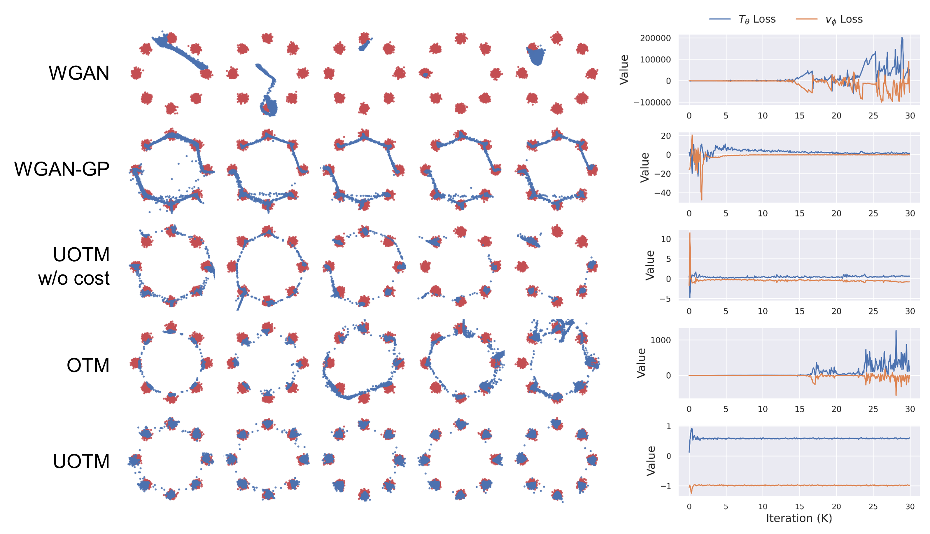
Figure 1: Comparison of Training Dynamics between OT-based GANs. Left: Visualization of generated samples (blue) and data samples (red) for every 6K iterations. Right: Training loss of the generator ($T_{\theta}$ Loss) and discriminator ($v_{\phi}$ Loss) for each algorithm.

3.2.1 Effect of Strictly Convex $g_{1}$ and $g_{2}$

Experimental Results

Fig 1 illustrates how each model evolves during training for each 6K iterations. To investigate the effect of $g_{1}$ and $g_{2}$, we compare the models with $g_{1}=g_{2}=\text{Id}$ (WGAN, OTM) and $g_{1}=g_{2}=\text{Sp}$ (UOTM, UOTM w/o cost). When $g_{1}=g_{2}=\text{Id}$, WGAN and OTM initially appear to converge in the early stages of training. However, as training progresses, the loss highly fluctuates, leading to divergent results. Interestingly, adding a gradient penalty regularizer to WGAN (WGAN-GP) is helpful in addressing this loss fluctuation. Conversely, when $g_{1}=g_{2}=\text{Sp}$, UOTM and UOTM w/o cost consistently perform well, with the loss steadily converging during training. From these observations, we interpret that setting $g_{1},g_{2}$ to Sp functions, which are strictly convex, contribute to the stable convergence of OT-based GANs.

Moreover, Tab 2 presents CIFAR-10 generation results under various backbone architectures: DCGAN (Radford et al., 2015) and NCSN++ (Song et al., 2021b). Here, we additionally compared UOTM (KL) following Choi et al. (2023a). UOTM (KL) serves as another example of strictly convex $g_{1},g_{2}$, where $g_{1}=g_{2}=e^{x}-1$. As in the toy dataset, UOTM w/o cost and UOTM outperform their algorithmic counterparts with respect to $g_{1},g_{2}$, i.e., WGAN and OTM, respectively. The additional stability of UOTM can be observed in an ablation study on the regularizer intensity $\lambda$ (Fig 3). UOTM model provides more robust FID results compared to OTM.

Effect of $g_{1}$ and $g_{2}$ in Optimization

We observed that the introduction of strictly convex functions, such as SP or $g(x)=e^{x}-1$, into $g_{1},g_{2}$ contributes to more stable training of OT-based GANs. We explain this enhanced stability in terms of the adaptive optimization of the potential network $v_{\phi}$. From the potential loss function $\mathcal{L}_{v}$ in line 5 of Algorithm 1, we can express the gradient descent update for the potential function $v_{\phi}$ with a learning rate $\gamma$ as follows:

$$\phi-\gamma\nabla_{\phi}\mathcal{L}_{v_{\phi}} =\phi-\frac{\gamma}{|X|}\sum_{x\in X}\underbrace{g_{1}^{\prime}(-\hat{l}(x))}_{=:\hat{w}(x)}\nabla_{\phi}v_{\phi}(\hat{y})+\frac{\gamma}{|Y|}\sum_{y\in Y}\underbrace{g_{2}^{\prime}\left(-v_{\phi}(y)\right)}_{=:w(y)}\nabla_{\phi}v_{\phi}(y),$$ (9)

where $\hat{l}(x)=c(x,\hat{y})-v_{\phi}(\hat{y})$. Note that the generator loss $\mathcal{L}_{T}=\frac{1}{|X|}\sum_{x\in X}\hat{l}(x)$, since we assume $g_{3}=\text{Id}$. Here, $w$ and $\hat{w}$ in Eq 9 serve as sample-wise weights for the potential gradient $\nabla_{\phi}v_{\phi}$.

We interpret the role of $g_{1},g_{2}$ as mediating the balance between $T$ and $v$. Suppose the generator dominates the potential for certain $x$, i.e., $\hat{l}(x)$ is small. In this case, because $g_{1}^{\prime}$ is a strictly increasing function, the weight $\hat{w}(x)$ becomes large for this sample $x$, counterbalancing the dominant generator. Similarly, consider the weight of the true data sample $w(y)$. Note that the goal of potential is to assign a high value to real data $y$ and a low value to generated samples $\hat{y}$. Assume that the potential is not good at discriminating certain $y$, which means that $v(y)$ is small. Then, the weight $w(y)$ becomes large for this sample $y$ as above. We hypothesize that this failure-aware adaptive optimization of the potential $v_{\phi}$ stabilizes the training procedure, regardless of the regularizer.

Table 2: FID Scores of OT-based GANs on CIFAR-10.

Model	Architecture
	DCGAN	NCSN++
WGAN	52.3	48.8
WGAN-GP	50.8	4.5
OTM	19.8	4.3
UOTM w/o cost	15.4	19.7
UOTM (SP)	15.8	2.7
UOTM (KL)	12.2	2.9

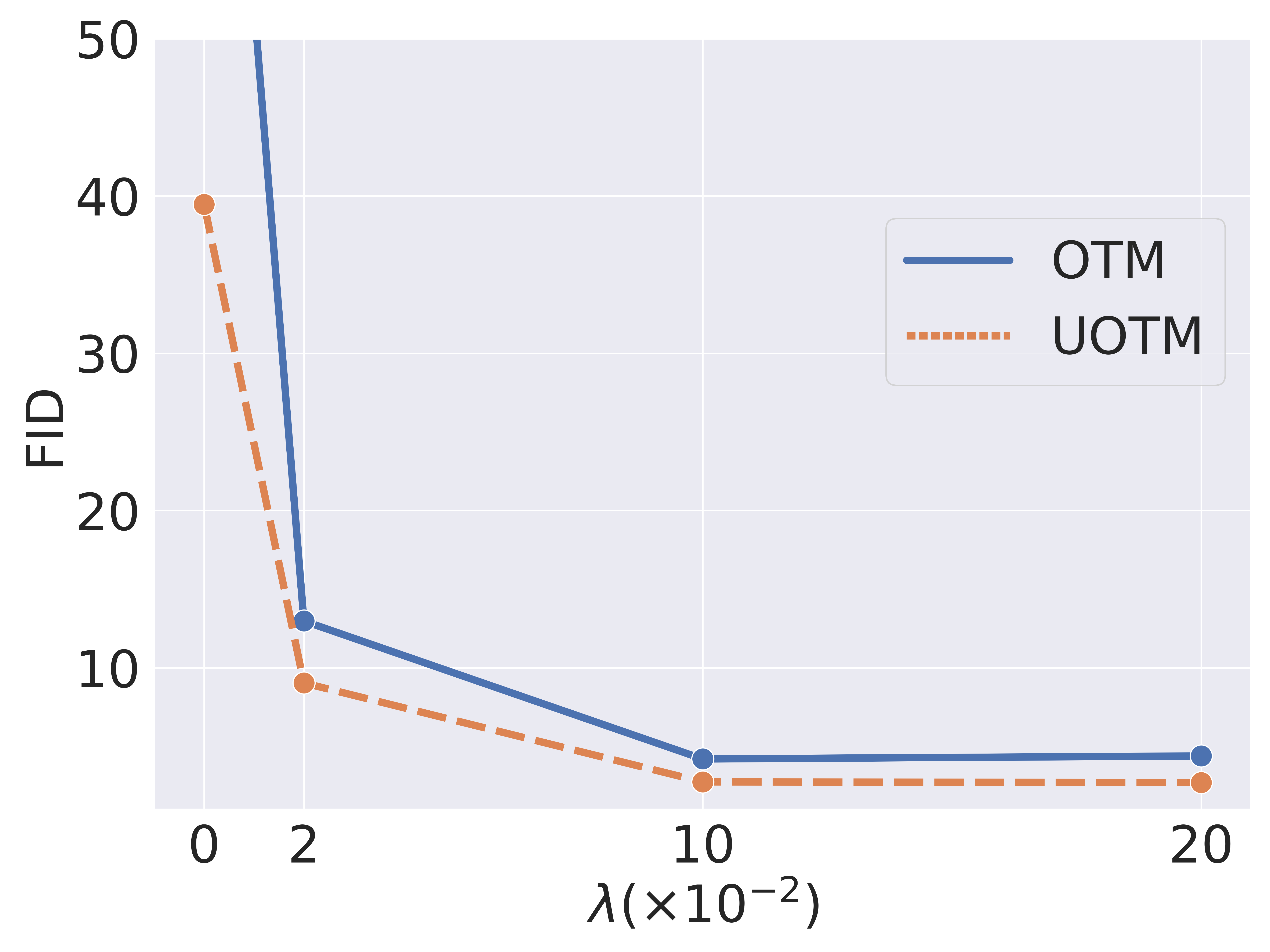
Figure 2: Ablation Study on Regularizer Intensity $\lambda$.

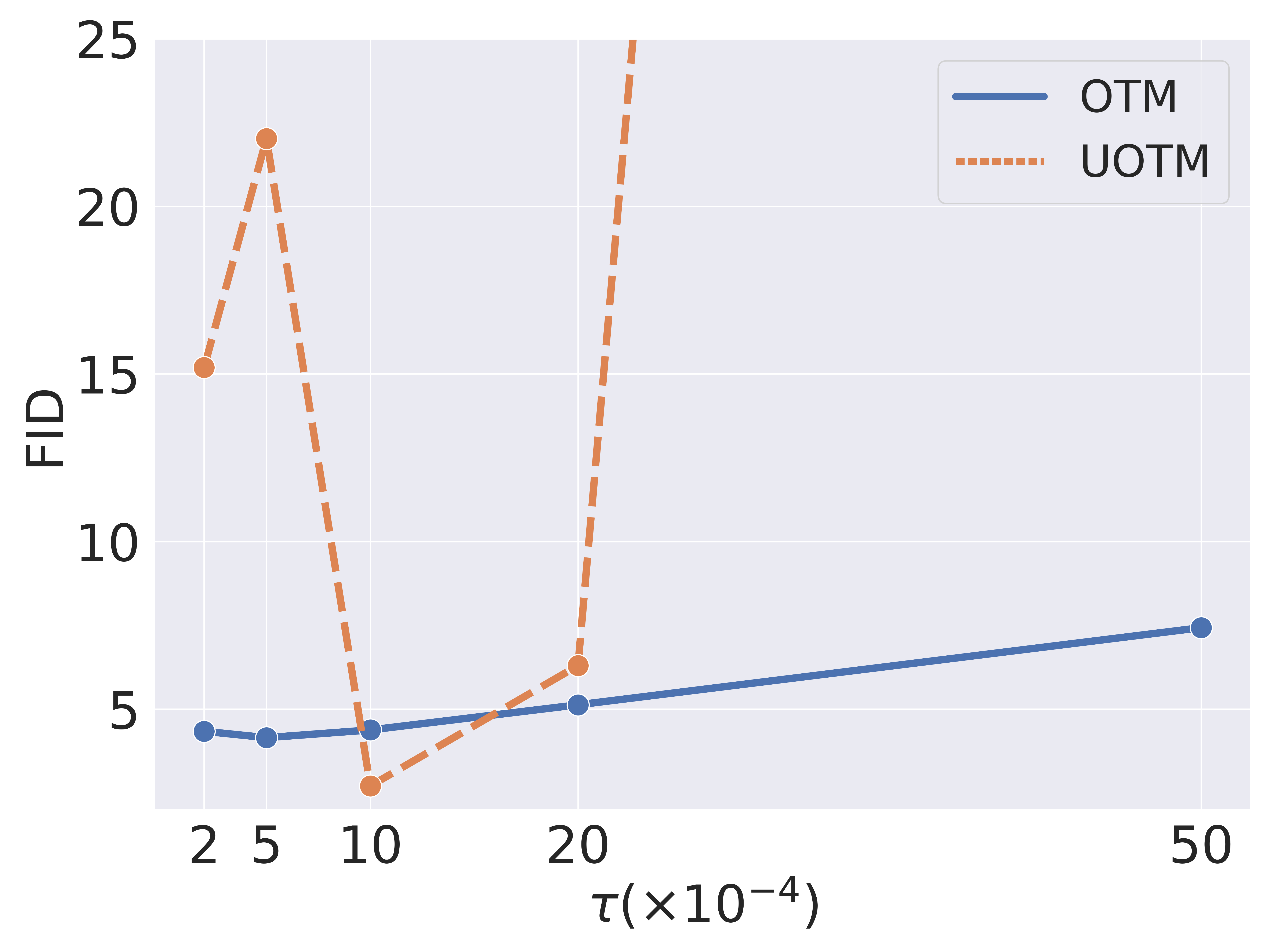
Figure 3: Ablation Study on Cost Intensity $\tau$.

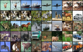
(a) Small $\tau$

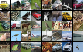
(b) Optimal $\tau$

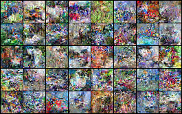
(c) Large $\tau$

Figure 4: Qualitative Comparison of Generated Samples from UOTM. Left: When $\tau$ is too small ($\tau=0.0002$). Middle: When $\tau$ is optimal ($\tau=0.001$). Right: When $\tau$ is too large ($\tau=0.005$). On Left, we reordered randomly generated samples to gather similar-looking samples. When $\tau$ is large, the samples appear noisy, and when $\tau$ is small, the generated samples show a mode collapse problem.

3.2.2 Effect of Cost Function

Experimental Results

To examine the effect of the cost function $c(x,y)=\tau\lVert x-y\rVert_{2}^{2}$, we compare the models with $\tau=0$ (WGAN, UOTM w/o cost) and $\tau>0$ (OTM, UOTM) in Fig 1. When $\tau=0$, both WGAN and UOTM w/o cost exhibit a mode collapse problem. These models fail to fit all modes of the data distribution. On the other hand, WGAN-GP shows a mode mixture problem. WGAN-GP generates inaccurate samples that lie between the modes of data distribution. In contrast, when $\tau>0$, both OTM and UOTM avoid model collapse and mixture problems. In the initial stages of training, OTM succeeds in capturing all modes of data distribution, until training instability occurs due to loss fluctuation. UOTM achieves the best distribution fitting by exploiting the stability of $g_{1},g_{2}$ as well. From these results, we interpret that the cost function $c(x,y)$ plays a crucial role in preventing mode collapse by guiding the generator towards cost-minimizing pairs.

Furthermore, we analyze the influence of the cost function intensity $\tau$ by performing an ablation study on $\tau$ on CIFAR-10 (Fig 3). Interestingly, the results are quite different between OTM and UOTM. When we compare the best-performing $\tau$, UOTM achieves much better FID scores than OTM ($\tau=10\times 10^{-4})$. However, when $\tau$ is excessively small or large, the performance of UOTM deteriorates severely. On the contrary, OTM maintains relatively stable results across a wide range of $\tau$. The deterioration of UOTM can be understood intuitively by examining the generated results in Fig 4. When $\tau$ is too large, UOTM tends to produce noise-like samples because the cost function dominates the other divergence terms $D_{\Psi_{i}}$ within the UOT objective (Eq 6). When $\tau$ is too small, UOTM shows a mode collapse problem because the negligible cost function fails to prevent the mode collapse. Conversely, as inferred from OT objective (Eq 1), the optimal pair $(v^{\star},T^{\star})$ of OTM remains consistent regardless of variations in $\tau$. Hence, OTM presents relatively consistent performance across changes in $\tau$ (Fig 3). In Sec 4, we propose a method that enhances the $\tau$-robustness of UOTM while also improving its best-case performance.

Effect of Cost in Mode Collapse/Mixture

In Fig 1, the OT-based GANs with the cost term (OTM, UOTM) exhibited a significantly lower occurrence of mode collapse/mixture, compared to the models without the cost term. This observation proves that the cost function plays a regularization role in OT-based GANs, helping to cover all modes within the data distribution. This cost function encourages the generator $T$ to minimize the quadratic error between input $x$ and output $T(x)$. In other words, the generator $T$ is indirectly guided to transport each input $x$ to a point, that is within the data distribution support and close to $x.$ Fig 5 visualizes the transported pair $(x,T(x))$ by the gray line that connects $x$ and $T(x)$. Fig 5 demonstrates that this cost term induces OTM and UOTM to spread the generated samples (in an optimal way).

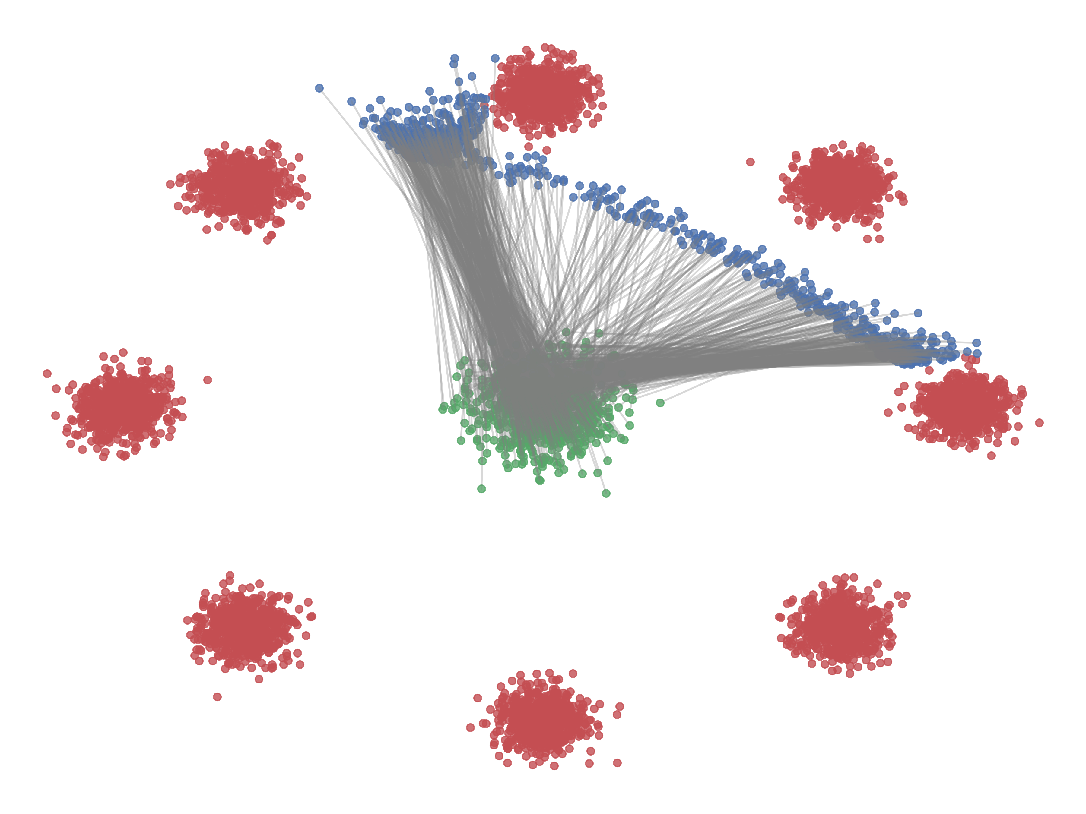
(a) WGAN

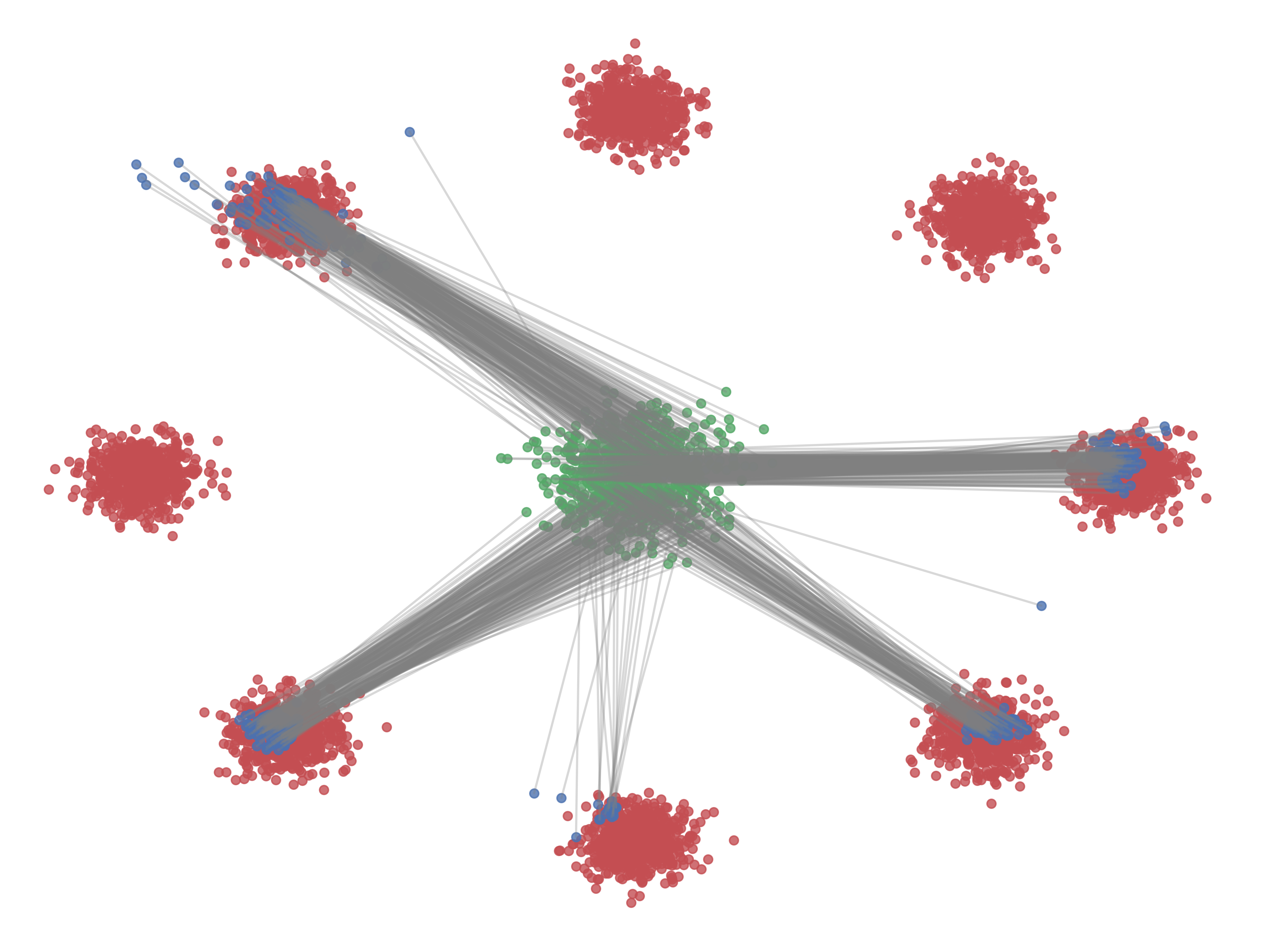
(b) UOTM w/o cost

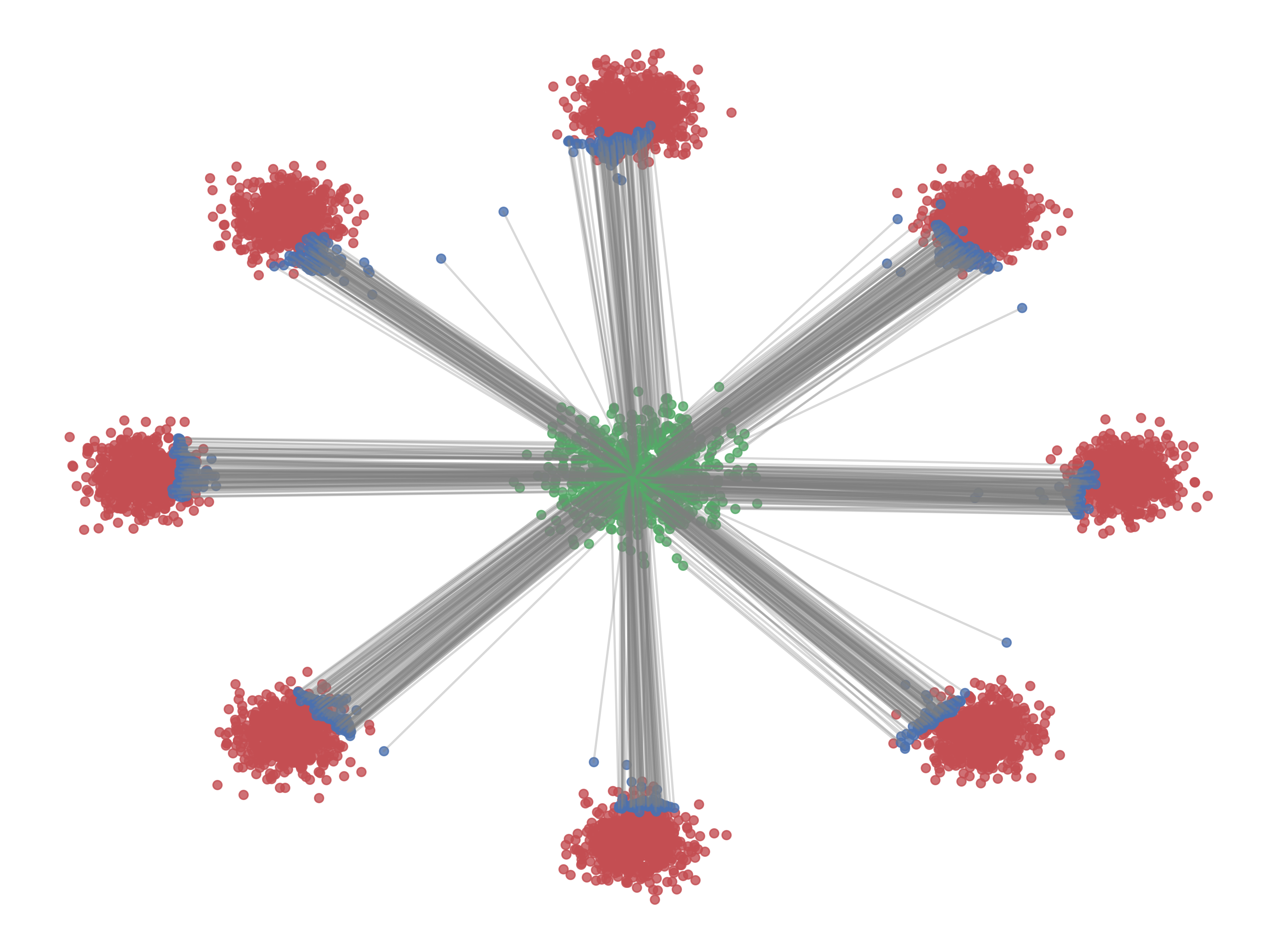
(c) OTM

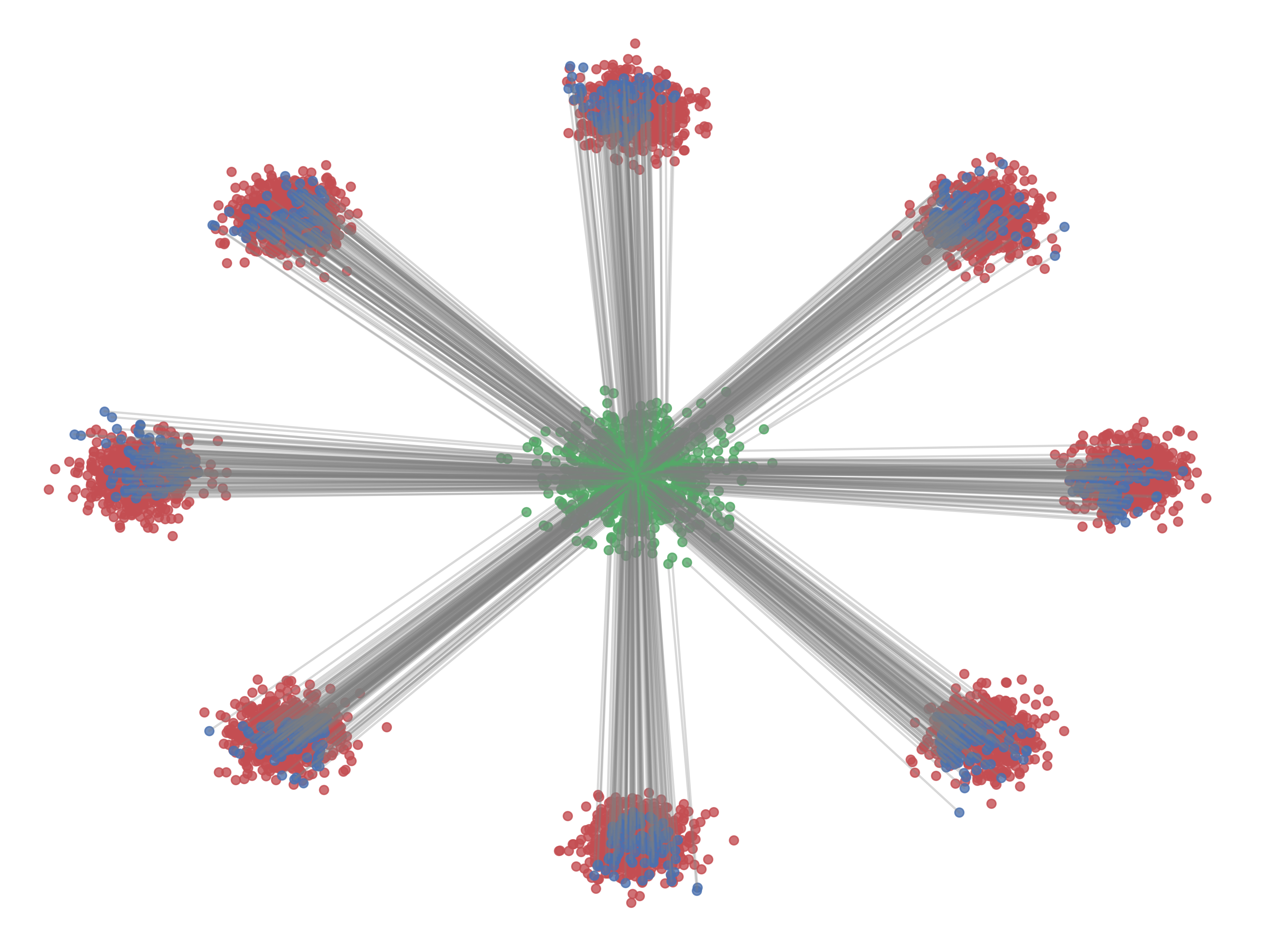
(d) UOTM

Figure 5: Visualization of Generator $T_{\theta}$. The gray lines illustrate the generated pairs, i.e., the connecting lines between $x$ (green) and $T_{\theta}(x)$ (blue). The red dots represent the training data samples.

3.2.3 Additional Advantage of UOTM

Lipshitz Continuity of UOTM Potential

Here, we offer an additional explanation for the stable convergence observed in UOTM. In OT-based GANs, we approximate the generator and potential with neural networks. However, since neural networks can only represent continuous functions, it is crucial to verify the regularity of these target functions, such as Lipschitz continuity. If these target functions are not continuous, the neural network approximation may exhibit highly irregular behavior. Theorem 3.1 proves that under minor assumptions on $g_{1}$ and $g_{2}$ employed in UOTM (Choi et al., 2023a), there exists unique optimal potential $v^{\star}$ and it satisfies Lipschitz continuity. (See Appendix A for the proof.)

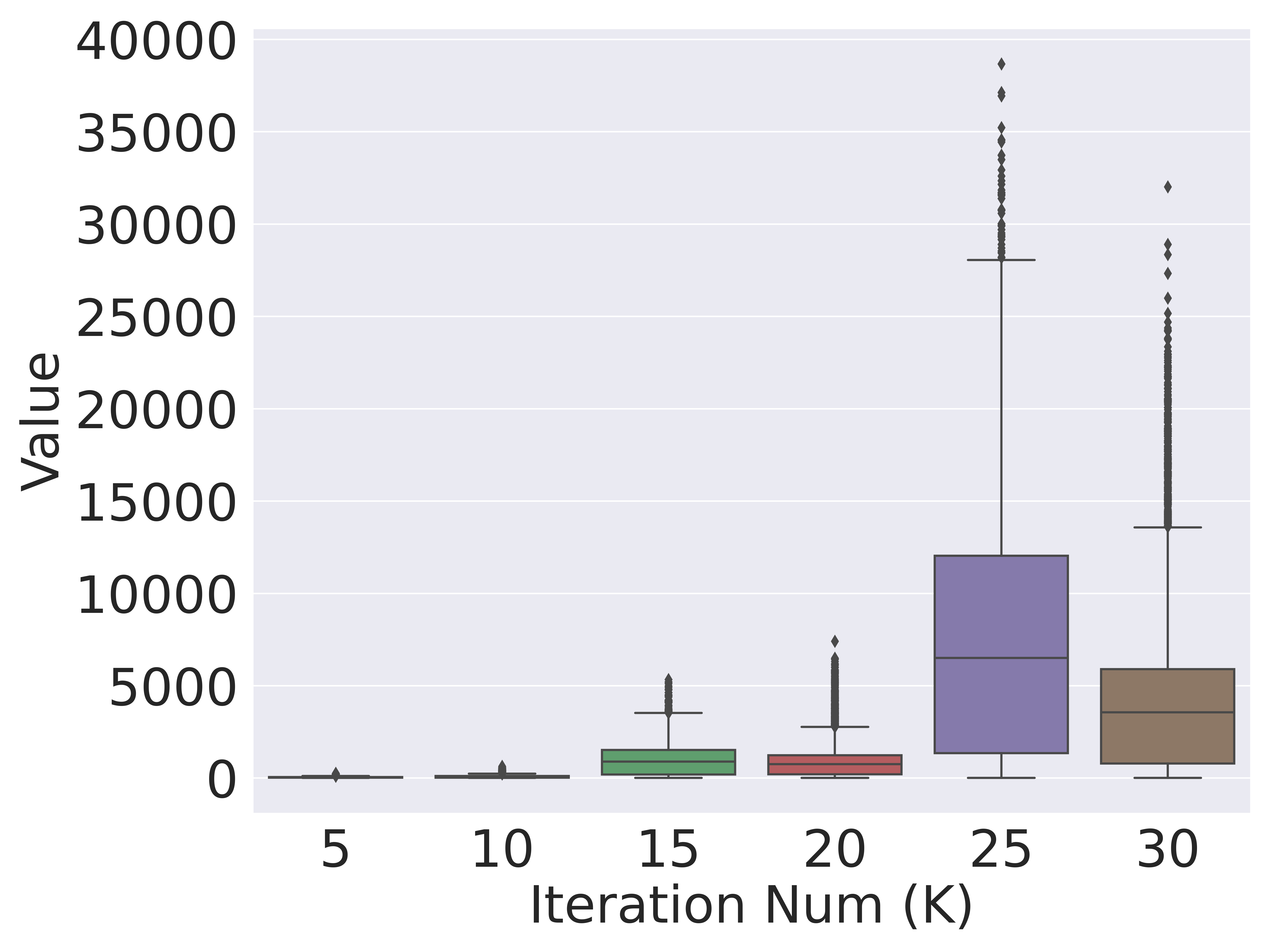
(a) WGAN

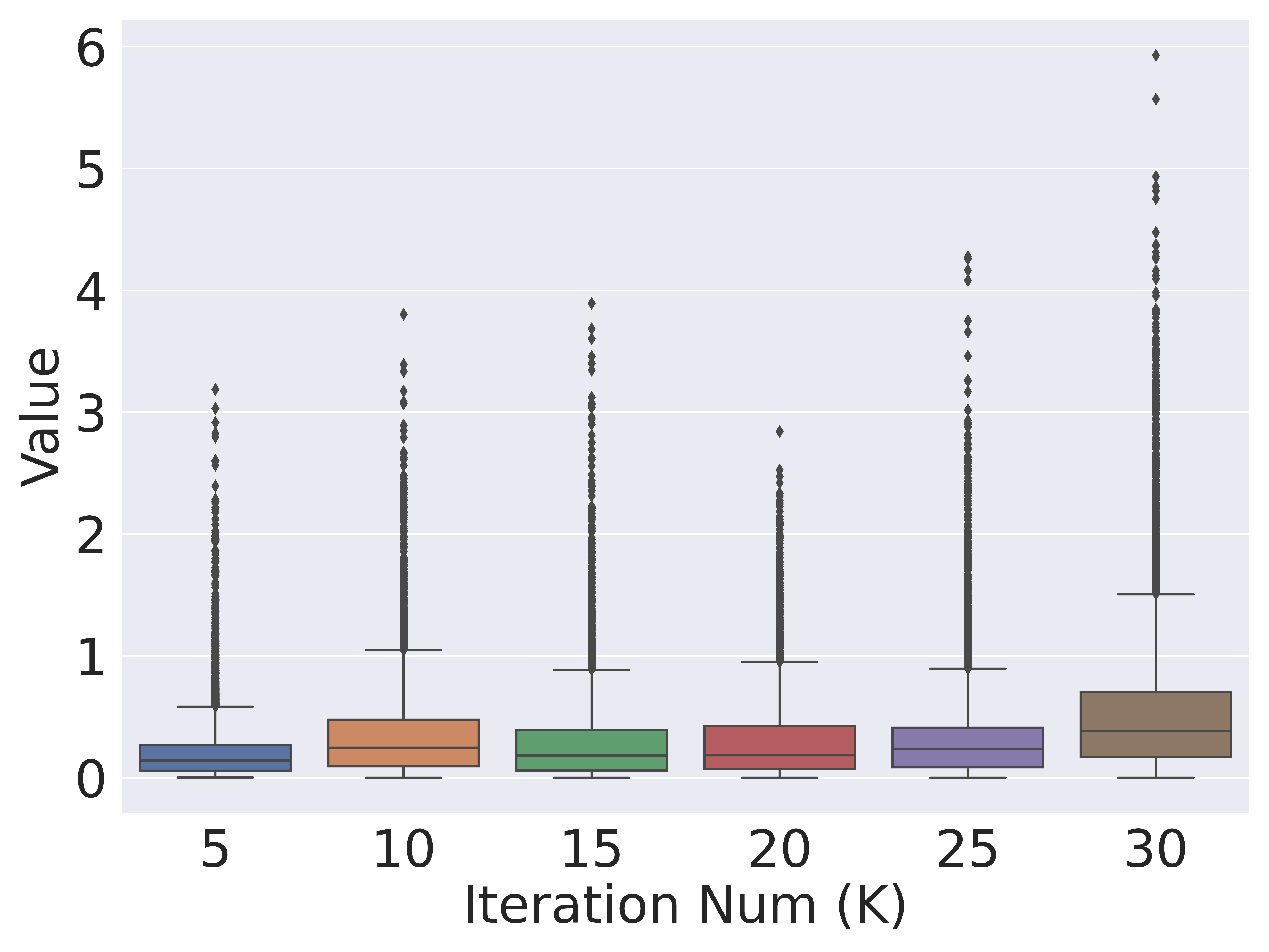
(b) UOTM w/o cost

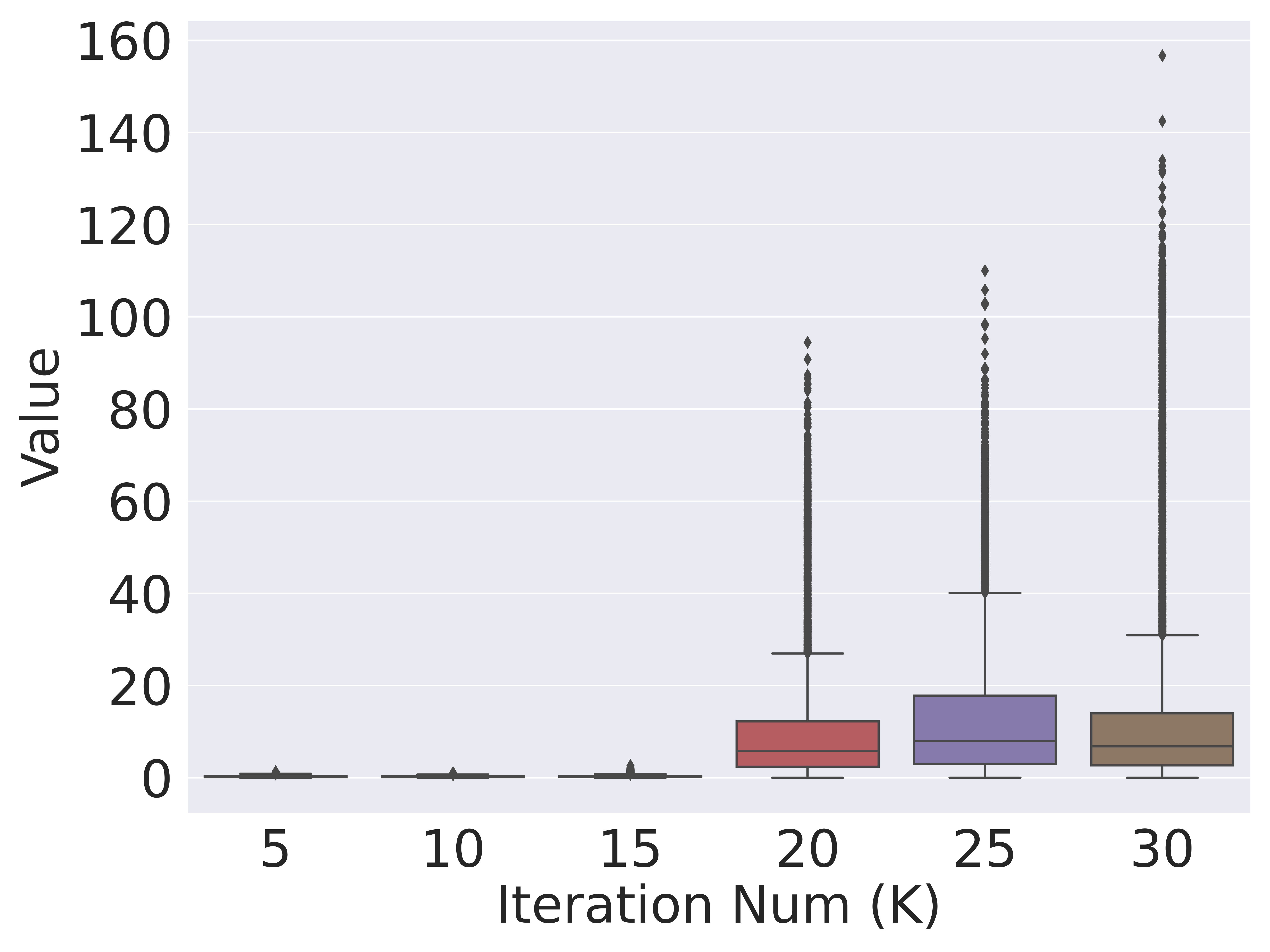
(c) OTM

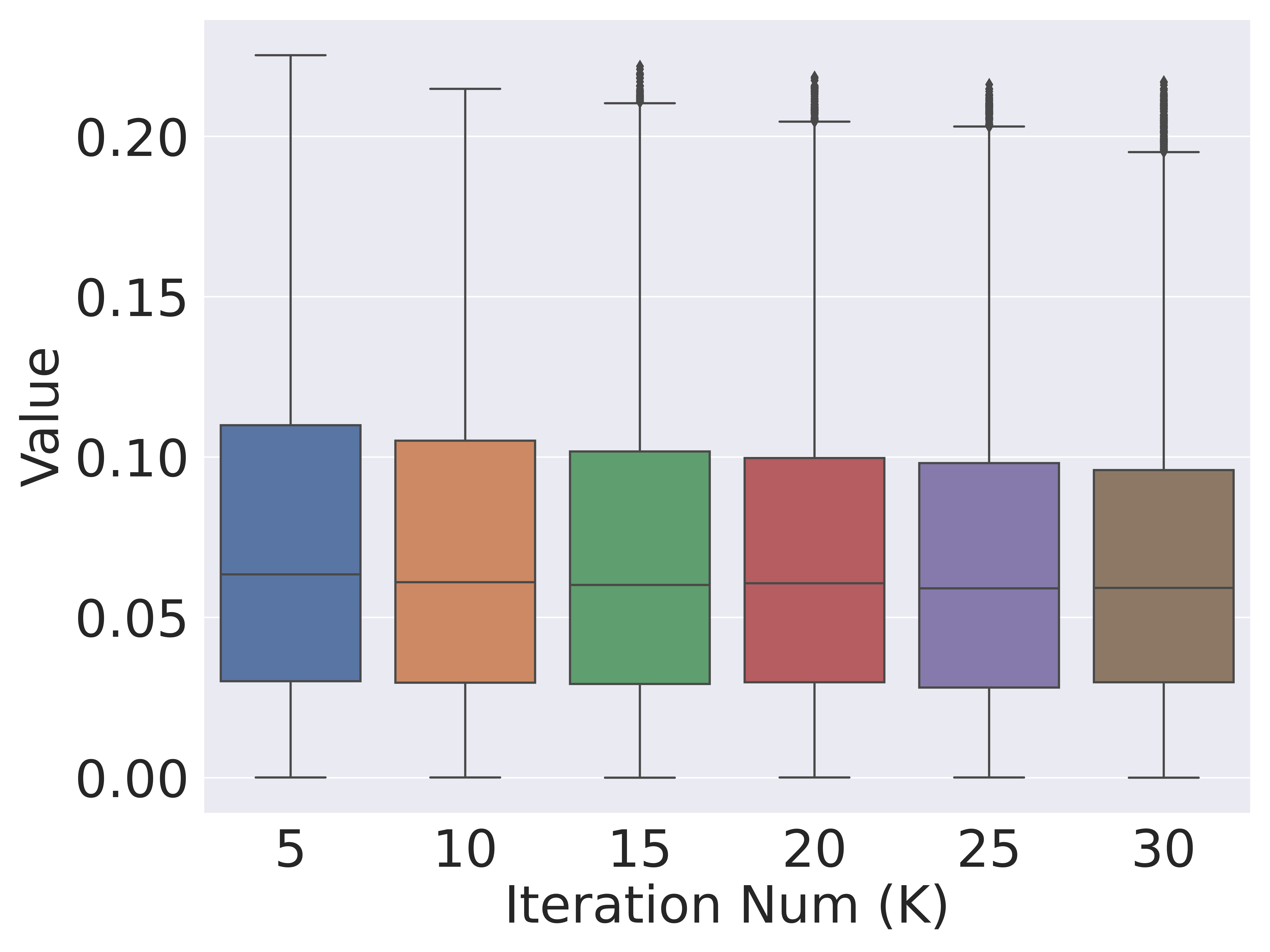
(d) UOTM

Figure 6: Distribution of the absolute value of Average Rate of Change (ARC) of potential $\frac{|v_{\phi}(y)-v_{\phi}(x)|}{\lVert y-x\rVert}$ for every 5K iterations. Due to the equi-Lipschitz property, $|\text{ARC}|$ of UOTM potential is stable during training. This stability contributes to the stable training of UOTM.

Theorem 3.1.

Let $g_{1}$ and $g_{2}$ be real-valued functions that are non-decreasing, bounded below, differentiable, and strictly convex. Assuming the regularity assumptions in Appendix A, there exists a unique Lipschitz continuous optimal potential $v^{\star}$ for Eq 7. Moreover, for the semi-dual maximization objective $-\mathcal{L}_{v}$ (Eq 7),

$$\Gamma:=\left\{v\in\mathcal{C}(\mathcal{Y}):\mathcal{L}_{v}\leq 0,v^{cc}=v\right\},$$ (10)

is equi-bounded and equi-Lipschitz.

Note that the semi-dual objective $\mathcal{L}_{v}$ can be derived by assuming the optimality of $T_{\theta}$ for given $v$, i.e., $T_{\theta}(x)\in\arg\inf_{y\in\mathcal{Y}}\left[c(x,y)-v\left(y\right)\right]$. Moreover, Theorem 3.1 shows that the set of valid potential candidates $\Gamma$ is equi-Lipschitz, i.e., there exists a Lipshitz constant $L_{\Gamma}$ that all $v\in\Gamma$ are $L_{\Gamma}$-Lipschitz. This equi-Lipschitz continuity also explains the stable training of UOTM. The condition $\mathcal{L}_{v}\leq 0$ in $\Gamma$ is not a tough condition for the neural network $v_{\phi}$ to satisfy during training, since $\mathcal{L}_{v}=0$ when $v\equiv 0$ . Therefore, during training, the potential network $v_{\phi}$ would remain within the domain of $L_{\Gamma}$-Lipshitz functions. In other words, $v_{\phi}$ would not express any drastic changes for all input $y$. Furthermore, the target of training, $v^{\star}$, also stays within this set of functions. Hence, we can expect stable convergence of the potential network as training progresses.

Experimental Validation

We tested whether this equi-Lipschitz continuity of UOTM potential $v_{\phi}$ is observed during training in practice. In particular, we randomly choose data $a\in\mathcal{Y}$ and $b\sim\nu$ on 2D experiment and visualize the Average Rate of Change (ARC) of potential $\frac{|v_{\phi}(b)-v_{\phi}(a)|}{\lVert b-a\rVert}$. Fig 6 shows boxplots of an ARC of ten thousand pairs of $(a,b)$ for every 10K iterations. As shown in Fig 6, only UOTM shows a bounded ARC, and others, especially WGAN and OTM, diverge as the training progresses. This result indirectly shows the potential network in UOTM mostly remains within the equi-Lipschitz set during training. Furthermore, we can conjecture that the highly irregular behavior of potential networks in other models could potentially disrupt stable training processes.

4 Towards the stable OT map

Table 3: Image Generation on CIFAR-10. $\dagger$ indicates the results conducted by ourselves.

Class	Model	FID ($\downarrow$)
GAN	SNGAN+DGflow (Ansari et al., 2020)	9.62
	StyleGAN2 w/o ADA (Karras et al., 2020)	8.32
	StyleGAN2 w/ ADA (Karras et al., 2020)	2.92
Diffusion	DDPM (Ho et al., 2020)	3.21
	Score SDE (VE) (Song et al., 2021b)	2.20
	Score SDE (VP) (Song et al., 2021b)	2.41
	DDIM (50 steps) (Song et al., 2021a)	4.67
	LSGM (Vahdat et al., 2021)	2.10
OT-based	WGAN (Arjovsky et al., 2017)	55.20
	WGAN-GP(Gulrajani et al., 2017)	39.40
	OTM † (Rout et al., )	4.15
	UOTM (Choi et al., 2023a)	2.97
	UOTM-SD (Cosine)†	2.57
	UOTM-SD (Linear)†	2.51
	UOTM-SD (Step)†	2.78

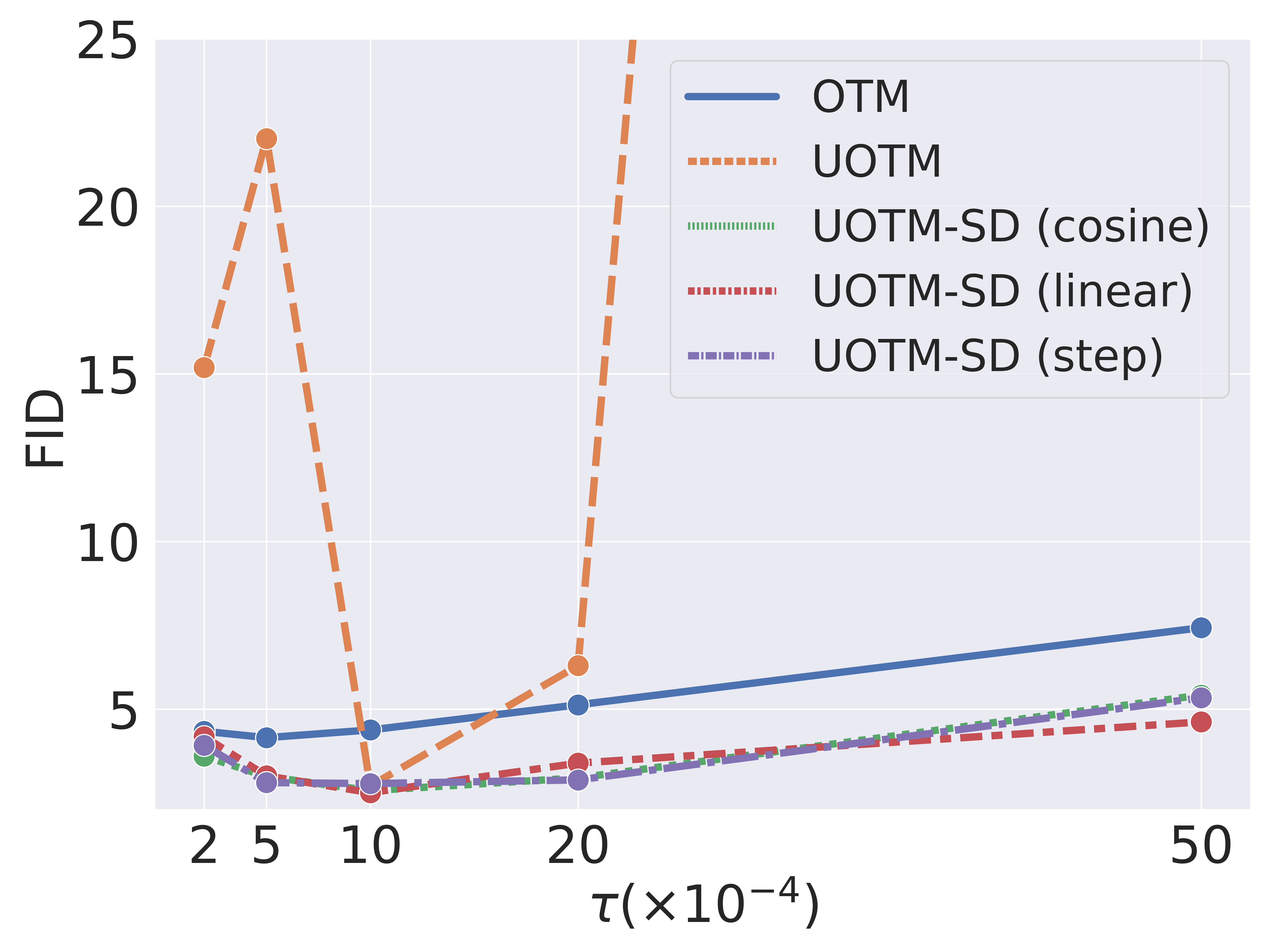
Figure 7: Comparison of $\tau$-robustness.

In this section, we suggest a straightforward yet novel method to enhance the $\tau$-robustness of UOTM, while improving the best-case performance. Intuitively, our idea is to gradually adjust the transport map in the UOT problem towards the transport map in the OT problem. Note that the OT problem of OTM assumes a hard constraint on marginal matching.

Motivation

The analysis in Sec 3 showed that the semi-dual form of the UOT problem, i.e., UOTM, provides several advantages over other OT-based GANs. However, Fig 4 showed that UOTM is $\tau$-sensitive. In this respect, Choi et al. (2023a) proved that the upper bound of marginal discrepancies for the optimal $\pi^{\star}$ in the UOT problem (Eq 6) is linearly proportional to $\tau$:

$$D_{\Psi_{1}}(\pi_{0}^{\star}|\mu)+D_{\Psi_{2}}(\pi_{1}^{\star}|\nu)\leq\tau\mathcal{W}_{2}^{2}(\mu,\nu)\quad\mathrm{for}\quad c(x,y)=\tau\lVert x-y\rVert_{2}^{2}.$$ (11)

When the divergence term is minor (Large $\tau$), the cost term prevents the mode collapse problem (Sec 3.2.2), but the model fails to match the target distribution, generating noisy samples (Eq 11). Conversely, when the divergence term is dominant (Small $\tau$), the model should theoretically exhibit improved target distribution matching (Eq 11, Theorem 4.1). However, the mode collapse problem disturbs the optimization process in practice (Sec 3.2.2). In this regard, we introduce a method that can leverage the advantages of both regimes: preventing mode collapse with minor divergence and improving distribution matching with dominant divergence. Intuitively, we start training with a smaller divergence term to mitigate mode collapse. Subsequently, as training progresses, we gradually increase the influence of the divergence term to achieve better data distribution matching.

Method

Formally, we consider the following $\alpha$-scaled UOT problem ($\alpha$-UOT) $C_{ub}^{\alpha}(\mu,\nu)$ for $\alpha\geq 0$ (Eq 12). Note that this $\alpha$-UOT problem recovers the OT problem $C(\mu,\nu)$ when $\alpha\rightarrow\infty$ if $\mu,\nu$ have equal mass (Fatras et al., 2021).

$$C_{ub}^{\alpha}(\mu,\nu)=\inf_{\pi^{\alpha}\in\mathcal{M}_{+}(\mathcal{X}\times\mathcal{Y})}\left[\int_{\mathcal{X}\times\mathcal{Y}}c(x,y)d\pi^{\alpha}(x,y)+\alpha D_{\Psi_{1}}(\pi_{0}^{\alpha}|\mu)+\alpha D_{\Psi_{2}}(\pi_{1}^{\alpha}|\nu)\right].$$ (12)

Motivated by this fact, we suggest a monotone-increasing scheduling scheme during training for $\alpha$ to achieve the stable convergence of the UOT transport map $\pi^{\alpha}$ towards the OT transport map. Because $\alpha D_{\Psi{i}}=D_{\alpha\Psi{i}}$ and $(\alpha\Psi_{i})^{*}(x)=\alpha\Psi_{i}^{*}(x/\alpha)$, the learning objective of $\alpha$-scaled UOTM are given as follows:

$$\mathcal{L}_{v_{\phi},T_{\theta}}^{\alpha}=\inf_{v_{\phi}}\left[\int_{\mathcal{X}}\alpha\Psi^{*}_{1}\left(-\frac{1}{\alpha}\inf_{T_{\theta}}\left[c(x,T_{\theta}(x))-v\left(T_{\theta}(x)\right)\right]\right)d\mu(x)+\int_{\mathcal{Y}}\alpha\Psi_{2}^{*}\left(-\frac{1}{\alpha}v(y)\right)\right].$$ (13)

Note that, given our assumption that $\Psi_{i}^{*}$ is $C^{1}$, $(\alpha\Psi_{i})^{*}$ uniformly converges to Id for every compact domain, since $\Psi_{i}^{*}(0)=0,(\Psi_{i}^{*})^{\prime}(0)=1$. Therefore, this $\alpha$-scheduling can be intuitively understood as a gradual process of straightening the strictly convex $\Psi_{i}^{*}$ function towards the identity function Id, so that $\mathcal{L}_{v_{\phi},T_{\theta}}^{\alpha}$ converges to OTM (Tab 1). We refer to this UOTM with $\alpha$-scheduling as UOTM with Scheduled Divergence (UOTM-SD).

Convergence

The next Theorem 4.1 proves that the optimal transport plan of the $\alpha$-scaled UOT problem converges to that of the OT problem as $\alpha\rightarrow\infty$. However, one limitation of this theorem is that it shows the convergence of transport plan $\pi$, but does not address the convergence of the transport map $T$.

Theorem 4.1.

Assume the entropy functions $\Psi_{1},\Psi_{2}$ are strictly convex and finite on $(0,\infty)$. Then, the optimal transport plan $\pi^{\alpha,\star}$ of the $\alpha$-scaled UOT problem $C_{ub}^{\alpha}(\mu,\nu)$ (Eq 6) weakly converges to the optimal transport plan $\pi^{\star}$ of the OT problem $C(\mu,\nu)$ (Eq 1) as $\alpha$ goes to infinity.

$\alpha$-schedule Settings

We evaluated three scheduling schemes for $\alpha$. Instead of directly adjusting (increasing) $\alpha$, we implemented a scheduling approach by tuning (decreasing) $\tilde{\alpha}=\alpha^{-1}$. For the schedule parameters $\alpha_{max}\geq\alpha_{min}>0$, the assessed scheduling schemes are as follows:

• Cosine : Apply Cosine scheduling for $\tilde{\alpha}=\alpha^{-1}$ from $\alpha_{min}^{-1}$ to $\alpha_{max}^{-1}$.

• Linear : Apply Linear scheduling for $\tilde{\alpha}=\alpha^{-1}$ from $\alpha_{min}^{-1}$ to $\alpha_{max}^{-1}$.

• Step : At each $t_{iter}$ iterations, multiply $\alpha$ by 2 until $\alpha=\alpha_{max}$.

We chose this approach for two reasons. Firstly, $\tilde{\alpha}$ provides a more intuitive interpretation of the allowed marginal discrepancy. For example, setting $\alpha=5$ in the $\alpha$-UOT is equivalent to multiplying $\tilde{\alpha}=0.2$ to $\tau$. Then, this adjustment results in a reduction in the upper bound of the marginal discrepancy, $\mathcal{W}_{2}^{2}(\mu,\nu)$, by a factor of $\tilde{\alpha}$ (Eq 11). Secondly, we can exploit various existing scheduling methods for other parameters, such as learning rate scheduling (Loshchilov & Hutter, 2017; He et al., 2016). These existing scheduling techniques typically work by decreasing the target parameters. Hence, when we consider $\tilde{\alpha}$, we can directly apply these existing methods.

Generation Results

We tested our UOTM-SD model on CIFAR-10 ($32\times 32$) dataset. For quantitative evaluation, we adopted FID (Heusel et al., 2017) score. Tab 3 shows that our UOTM-SD improves UOTM (Choi et al., 2023a) across all three scheduling schemes. Our UOTM-SD achieves a FID of 2.51 under the best setting of linear scheduling with $(\alpha_{min},\alpha_{max})=(1/5,5)$ and $\tau=1\times 10^{-3}$, surpassing all other OT-based methods. We added a more extensive comparison with other generative models in Appendix D.1. (Due to page constraints, we included the ablation study regarding schedule intensity, i.e., $(\alpha_{min},\alpha_{max})$, and the schedule itself, i.e., $\alpha_{min}=\alpha_{max}$, in Appendix D.2.)

$\tau$ Robustness

We assessed the robustness of our model regarding the intensity parameter $\tau$ of the cost function $c(x,y)$. Specifically, we tested whether our UOTM-SD resolves the $\tau$-sensitivity of UOTM, observed in Fig 3. Fig 7 displays FID scores of UOTM-SD, UOTM, and OTM for various values of $\tau$. Note that we employed harsh conditions for $\tau$-robustness, where $\tau_{max}/\tau_{min}=25$. We adopted $\alpha_{min}=1/5$ and $\alpha_{max}=5$ for each UOTM-SD. All three versions of UOTM-SD outperform UOTM and OTM under the same $\tau$. While UOTM shows large variation of FID scores depending on $\tau$, ranging from $2.71$ to $218.02$, UOTM-SD provides much more stable results. (See Appendix D.1 for table results.)

5 Conclusion

In this paper, we integrated and analyzed various OT-based GANs. Our analysis unveiled that establishing $g_{1}$ and $g_{2}$ as lower-bounded, non-decreasing, and strictly convex functions significantly enhances training stability. Moreover, the cost function $c$ contributes to alleviating mode collapse and mixture problems. Nevertheless, UOTM, which leverages these two factors, exhibits $\tau$-sensitivity. In this regard, we suggested a novel approach that addresses this $\tau$-sensitivity of UOTM while achieving improved best-case results. However, there are some limitations to our work. Firstly, we fixed $g_{3}=\text{Id}$ during our analysis. Also, our convergence theorem for $\alpha$-scaled UOT guarantees the convergence of the transport plan, but not the transport map. Exploring these issues would be promising future research.

Reproducibility

To ensure the reproducibility of this work, we submitted the source code in the supplementary materials. The implementation details of all experiments are clarified in Appendix B. Moreover, the assumptions and complete proofs for Theorem 3.1 and 4.1 are included in Appendix A.

Appendix A Proofs

Notations and Assumptions

Let $\mathcal{X}$ and $\mathcal{Y}$ be compact complete metric spaces which are convex subsets of $\mathbb{R}^{d}$, and $\mu$, $\nu$ be positive Radon measures of the mass 1. For a measurable map $T:\mathcal{X}\rightarrow\mathcal{Y}$, $T_{\#}\mu$ denotes the associated pushforward distribution of $\mu$. $c(x,y)$ refers to the transport cost function defined on $\mathcal{X}\times\mathcal{Y}$. We assume $\mathcal{X},\mathcal{Y}\subset\mathbb{R}^{d}$ and the quadratic cost $c(x,y)=\tau\lVert x-y\rVert_{2}^{2}$, where $\tau$ is a given positive constant. Let $\Psi_{1}$ and $\Psi_{2}$ be an entropy function, i.e. $\Psi_{i}:\mathbb{R}\rightarrow[0,\infty]$ is a convex, lower-semi continuous, non-negative function such that $\Psi_{i}(1)=0$, and $\Psi_{i}(x)=\infty$ for $x<0$. Let $g_{1}:=\Psi^{*}$ and $g_{2}:=\Psi^{*}$ be a convex, differentiable, non-decreasing function defined on $\mathbb{R}$. We assume that $g_{1}(0)=g_{2}(0)=0$ and $g_{1}^{\prime}(0)=g_{2}^{\prime}(0)=1$.

Theorem A.1.

Let $g_{1}$ and $g_{2}$ be real-valued functions that are non-decreasing, bounded below, differentiable, and strictly convex. Assuming the regularity assumptions in Appendix A, there exists a unique Lipschitz continuous optimal potential $v^{\star}$ for Eq 7. Moreover, for the maximization objective $-\mathcal{L}_{v}$ of Eq 7,

$$\Gamma:=\left\{v\in\mathcal{C}(\mathcal{Y}):\mathcal{L}_{v}\leq 0,v^{cc}=v\right\},$$ (14)

is equi-bounded and equi-Lipschitz.

Proof.

Let

$$\mathcal{L}(v)=\int_{\mathcal{X}}g_{1}\left(-v^{c}(x))\right)d\mu(x)+\int_{\mathcal{Y}}g_{2}(-v(y))d\nu(y).$$ (15)

Since $\mathcal{L}(0)=0$, the infimum of $\mathcal{L}(v)$ is non-positive. Thus, $\Gamma$ is nonempty. We would like to prove that the set $\Gamma$ is equi-bounded and equi-Lipschitz, i.e., there exists a constant $L>0$ such that for every $z\in\Gamma$, $v^{c}|_{\text{supp}(\mu)}$ and $v|_{\text{supp}(\nu)}$ are $L$-Lipschitz. Let $A$ be the lower bound of functions $g_{1}$ and $g_{2}$, i.e. $A\leq g_{1}(x)$ and $A\leq g_{2}(y)$ for $x\in\mathcal{X}$ and $y\in\mathcal{Y}$, respectively. Furthermore, since $\mathcal{X}$ and $\mathcal{Y}$ are compact, there exists $M>0$ such that $c(x,y)\leq M$ for all $(x,y)\in\mathcal{X}\times\mathcal{Y}$. Then, since $g_{1}(x)\geq\text{Id}(x)$,

$$0\geq\mathcal{L}(v) \geq\int_{\mathcal{X}}-\inf_{y\in\mathcal{Y}}\left(c(x,y)-v(y)\right)d\mu(x)+\int_{\mathcal{Y}}g_{2}(-v(y))d\nu(y),$$ (16)

$$\geq-M+\underbrace{\sup_{y\in\mathcal{Y}}\left(v(y)\right)}_{=:\tilde{v}}+\int_{\mathcal{Y}}g_{2}(-v(y))d\nu(y)\geq-M+\tilde{v}+A,$$ (17)

which indicates that $v(y)\leq M-A$ for all $y\in\mathcal{Y}$. Note that $M$ nor $A$ is dependent on the choice of $v$. Thus, $v\in\Gamma$ is equi-bounded above. Moreover, by using similar logic with respect to $v^{c}$, we can easily prove that $v$ is also equibounded below. Consequently, by symmetricity, $v$ and $v^{c}$ are equi-bounded.

We now prove that there exists a uniform constant $L$ such that for every $z\in\Gamma$, $v$ is Lipschitz continuous with constant $L$. Since $v$ is bounded and $v^{cc}=v$, there exists a point $x(y)$ such that

$$v(y)=c(x(y),y)-v^{c}(x(y)),$$ (18)

and for every $\tilde{y}\in\mathcal{Y}$,

$$v(\tilde{y})\leq c(x(y),\tilde{y})-v^{c}(x(y)).$$ (19)

Subtracting the two previous inequalities gives,

$$v(\tilde{y})-v(y)\leq c(x(y),\tilde{y})-c(x(y),y).$$ (20)

Since $c$ is Lipschitz continuous on the compact domain $\mathcal{X}\times\mathcal{Y}$, there exists a Lipshitz constant $L$ that satisfies $|c(x(y),\tilde{y})-c(x(y),y)|\leq L\lVert\tilde{y}-y\rVert_{2}$. Thus,

$$|v(\tilde{y})-v(y)|\leq L\lVert\tilde{y}-y\rVert_{2}.$$ (21)

To sum up, $\Gamma$ is nonempty, equibounded, and equi-Lipschitz. Moreover, $\mathcal{L}(v)\geq 2A$, thus $\mathcal{L}(\Gamma)$ is lower-bounded.

Now, we would like to prove the compactness of $\Gamma$. Take any sequence $\{v_{n}\}_{n\in\mathbb{N}}\subset\Gamma$. Then, since $\Gamma$ is nonempty, equibounded, and equi-Lipschitz, we can obtain a uniformly convergent subsequence $\{v_{n_{k}}\}_{k\in\mathbb{N}}\rightarrow v$ by Arzelà-Ascoli theorem. Because $v_{n}(y)-\tau\lVert y\rVert_{2}^{2}$ is concave for each $v_{n}\in\Gamma$ from $v^{cc}=v$ (Santambrogio, 2015), $v$ is also continuous and $v(y)-\tau\lVert y\rVert_{2}^{2}$ is concave. Thus, $v$ is c-concave, i.e. $v^{cc}=v$. Now, to prove $v\in\Gamma$, we only need to prove $\mathcal{L}_{v}\leq 0$. Since $\{v_{n_{k}}\}_{k\in\mathbb{N}}\rightarrow v$ uniformly, it is easy to show that $\{v_{n_{k}}^{c}\}_{k\in\mathbb{N}}\rightarrow v^{c}$ uniformly. Moreover, note that $\{v_{n_{k}}^{c}\}_{k\in\mathbb{N}}$ is equibounded. By applying the dominated convergence theorem (DCT), we can easily prove that $\mathcal{L}_{v}\leq 0$. Thus, for any sequence of $\Gamma$, there exists a subsequence that converges to point of $\Gamma$ (Bolzano-Weierstrass property), which implies that $\Gamma$ is compact. Finally, since $\mathcal{L}(\Gamma)$ is lower-bounded, there exists a minimizer $v^{\star}\in\Gamma$, i.e. $\mathcal{L}(v^{\star})\leq\mathcal{L}(v)$ for all $v\in\Gamma$ by compactness of $\Gamma$.

Now, we prove the uniqueness of the minimizer. Let $K>0$ be a real value that $|v|\leq K$ and $|v^{c}|\leq K$ for every $v\in\Gamma$. There exists such $K$ by the equiboundedness. Now, let $\mathcal{C}_{K}$ denote the collection of continuous functions which are bounded by $K$. Since $g_{1}$ and $g_{2}$ are strictly convex on $[-K,K]$, the following dual minimization problem becomes strictly convex:

$$\inf_{(u,v)\in\mathcal{C}_{K}(\mathcal{X})\times\mathcal{C}_{K}(\mathcal{Y})}\int_{\mathcal{X}}g_{1}\left(-u(x))\right)d\mu(x)+\int_{\mathcal{Y}}g_{2}(-v(y))d\nu(y).$$ (22)

Thus, there exists at most one solution. Because there exists a solution $({v^{\star}}^{c},v^{\star})$, it is the unique solution. ∎

Theorem A.2.

Assume the entropy functions $\Psi_{1},\Psi_{2}$ are strictly convex and finite on $(0,\infty)$. Then, the optimal transport plan $\pi^{\alpha,\star}$ of the $\alpha$-scaled UOT problem $C_{ub}^{\alpha}(\mu,\nu)$ (Eq 6) weakly converges to the optimal transport plan $\pi^{\star}$ of the OT problem $C(\mu,\nu)$ (Eq 1) as $\alpha$ goes to infinity.

Proof.

Note that the $\alpha$-scaled UOT problem $C_{ub}^{\alpha}(\mu,\nu)$ is equivalent to setting the cost intensity $\tau\rightarrow\frac{\tau}{\alpha}$ within the cost function $c(x,y)=\tau\|x-y\|_{2}^{2}$ of the standard UOT problem $C_{ub}(\mu,\nu)$:

$$\pi^{\alpha,\star} ={\arg\inf}_{\pi^{\alpha}\in\mathcal{M}_{+}(\mathcal{X}\times\mathcal{Y})}\left[\int_{\mathcal{X}\times\mathcal{Y}}\tau\|x-y\|_{2}^{2}d\pi^{\alpha}(x,y)+\alpha D_{\Psi_{1}}(\pi_{0}^{\alpha}|\mu)+\alpha D_{\Psi_{2}}(\pi_{1}^{\alpha}|\nu)\right],$$ (23)

$$={\arg\inf}_{\pi\in\mathcal{M}_{+}(\mathcal{X}\times\mathcal{Y})}\left[\int_{\mathcal{X}\times\mathcal{Y}}\frac{\tau}{\alpha}\|x-y\|_{2}^{2}d\pi(x,y)+D_{\Psi_{1}}(\pi_{0}|\mu)+D_{\Psi_{2}}(\pi_{1}|\nu)\right].$$ (24)

Choi et al. (2023a) proved that, in the standard UOT problem, the marginal discrepancies for the optimal $\pi^{\star}$ are linearly proportional to the cost intensity. This relationship can be interpreted as follows for the above $\pi^{\alpha,\star}$:

$$D_{\Psi_{1}}(\pi_{0}^{\alpha,\star}|\mu)+D_{\Psi_{2}}(\pi_{1}^{\alpha,\star}|\nu)\leq\frac{\tau}{\alpha}\mathcal{W}_{2}^{2}(\mu,\nu).$$ (25)

Therefore, as $\alpha$ goes to infinity, the marginal distributions of $\pi^{\alpha,\star}$ converge in the Csiszàr divergences to the source $\mu$ and target $\nu$ distributions:

$$\lim_{\alpha\rightarrow\infty}D_{\Psi_{1}}(\pi_{0}^{\alpha,\star}|\mu)=\lim_{\alpha\rightarrow\infty}D_{\Psi_{2}}(\pi_{1}^{\alpha,\star}|\nu)=0.$$ (26)

The convergence in Csiszar divergence $D_{\Psi_{i}}$ for a strictly convex $\Psi_{i}$ implies the convergence of measures in Total Variation distance (Sason & Verdú, 2016; Csiszár, 1972). Then, this convergence in Total Variation distance implies the weak convergence of measures. This can be easily shown as follows: For any continuous and bounded $f\in\mathcal{C}_{b}(\mathcal{X})$, we have

$$\left|\int fd\mu_{n}-\int fd\mu\right|=\left|\int fd\left(\mu_{n}-\mu\right)\right| =\|f\|_{\infty}\left|\int(f/\|f\|)d\left(\mu_{n}-\mu\right)\right|,$$ (27)

$$\leq\|f\|_{\infty}\left\|\mu_{n}-\mu\right\|_{TV}.$$ (28)

Therefore, $\pi_{0}^{\alpha,\star}$ and $\pi_{1}^{\alpha,\star}$ weakly converges to $\mu$ and $\nu$, respectively. Choi et al. (2023a) showed that the optimal $\pi^{\alpha,\star}$ of Eq 24 becomes the optimal transport plan for the OT problem $C(\pi_{0}^{\alpha,\star},\pi_{1}^{\alpha,\star})$ for the same cost function $c(x,y)=\tau\|x-y\|_{2}^{2}$. (The optimal transport plan is invariant to the constant scaling of the cost function). Moreover, since $\mathcal{X},\mathcal{Y}$ are compact, $c(x,y)$ is bound on $\mathcal{X}\times\mathcal{Y}$. Thus,

$$\liminf_{\alpha\rightarrow\infty}\int c(x,y)d\pi^{\alpha,\star}<\infty.$$ (29)

Consequently, Theorem 5.20 from Villani et al. (2009) proves that $\pi^{\alpha,\star}$ weakly converges to the optimal transport plan $\pi^{\star}$ of the OT problem $C(\mu,\nu)$ as $\alpha$ goes to infinity.

∎

Appendix B Implementation Details

For every implementation, the prior (source) distribution is a standard Gaussian distribution with the same dimension as the data (target) distribution.

2D Experiments

For $m_{i}=12\left(\cos{\frac{i}{4}\pi},\sin{\frac{i}{4}\pi}\right)$ for $i=0,1,\dots,7$ and $\sigma=0.4$, we set mixture of $\mathcal{N}(m_{i},\sigma^{2})$ a target distribution. For all synthetic experiments, we used the same generator and discriminator network architectures. The auxiliary variable $z$ has a dimension of two. For a generator, we passed $z$ through two fully connected (FC) layers with a hidden dimension of 128, resulting in 128-dimensional embedding. We also embedded data $x$ into the 128-dimensional vector by passing it through three-layered ResidualBlock (Song & Ermon, 2019). Then, we summed up the two vectors and fed them to the final output module. The output module consisted of two FC layers. For the discriminator, we used three layers of ResidualBlock and two FC layers (for the output module). The hidden dimension is 128. Note that the SiLU activation function is used. We used a batch size of 128, and a learning rate of $2\times 10^{-4}$ and $10^{-4}$ for the generator and discriminator, respectively. We trained for 30K iterations. For OTM and UOTM, we chose the best results between settings of $\tau=0.01,0.05$. OTM has shown the best performance with $\tau=0.05$ and UOTM has shown the best performance with $\tau=0.01$. For WGANs and OTM, since they do not converge without any regularization, we set the regularization parameter $\lambda=5$. We used a gradient clip of $0.1$ for WGAN.

CIFAR-10

For the DCGAN model, we employed the architecture of Balaji et al. (2020), which uses convolutional layers with residual connection. Note that this is the same model architecture as in Rout et al. ; Choi et al. (2023a). We set a batch size of 128, 50K iterations, a learning rate of $2\times 10^{-4}$ and $10^{-4}$ for the generator and discriminator, respectively. For the NCSN++ model, we followed the implementation of Choi et al. (2023b) unless otherwise stated. We trained for 200K for OTM and 120K for other models because OTM converges slower than other models. Moreover, we used $R_{1}$ regularization of $\lambda=0.2$ for all methods and architectures. WGANs are known to show better performance with the optimizers without momentum term, thus, we use Adam optimizer with $\beta_{1}=0$, for WGANs. Furthermore, since OTM has a similar algorithm to WGAN, we also use Adam optimizer with $\beta_{1}=0$. Lastly, following Choi et al. (2023a), we use Adam optimizer with $\beta_{1}=0.5$ for UOTM. Note that for all experiments, we use $\beta_{2}=0.9$ for the optimizer. We used a gradient clip of $0.1$ for WGAN. Furthermore, the implementation of UOTM-SD follows the UOTM hyperparameter unless otherwise stated. We trained UOTM-SD for 200K iterations. For UOTM-SD (Cosine) and (Linear), we initiated the scheduling strategy from the start and finished the scheduling at 150K iterations. For UOTM-SD (Step), we halved $\tilde{\alpha}$ for every 30K iterations until it reaches $\alpha_{max}^{-1}$.

Evaluation Metric

For the evaluation of image datasets, we used 50,000 generated samples to measure FID (Karras et al., 2018) scores. For every model, we evaluate the FID score for every 10K iterations and report the best score among them.

Appendix C Problems of GAN-based Generative Models

Unstable training

Training adversarial networks involves finding a Nash equilibrium (Osborne & Rubinstein, 1994) in a two-player non-cooperative game, where each player aims to minimize their own objective function. However, discovering a Nash equilibrium is an exceedingly challenging task (Salimans et al., 2016; Mescheder et al., 2018). The prevailing approach for adversarial training is to adopt alternating gradient descent updates for the generator and discriminator. Unfortunately, the gradient descent algorithm often struggles to converge for many GANs (Salimans et al., 2016; Mescheder et al., 2018). Notably, Mescheder et al. (2018) showed that neither WGANs nor WGANs with Gradient Penalty (WGAN-GP) offer stable convergence.

Mode collapse/mixture

Another primary challenge in adversarial training is mode collapse and mixture phenomena. Mode collapse means that a generative model fails to encompass all modes of the data distribution. Conversely, mode mixture represents that a generative model fails to separate two modes of data distribution while attempting to cover all modes. This results in the generation of spurious or ambiguous samples. Many state-of-the-art GANs enforce regularization on the spectral norm (Miyato et al., ) to mitigate training instability. Odena et al. (2018) showed that enforcing the magnitude of the spectral norm of the networks reduces instability in training. However, recent works (Nagarajan & Kolter, 2017; Khayatkhoei et al., 2018; An et al., 2019; Salmona et al., 2022) have revealed that such Lipschitz constraints can lead the generator to concentrate solely on one of the modes or lead to mode mixtures in the generated samples.

Appendix D Additional Results

D.1 Full Table Result for CIFAR-10 Generation

Table 4: Image Generation on CIFAR-10. $\dagger$ indicates the results conducted by ourselves.

Class	Model	FID ($\downarrow$)
GAN	SNGAN+DGflow (Ansari et al., 2020)	9.62
	AutoGAN (Gong et al., 2019)	12.4
	TransGAN (Jiang et al., 2021)	9.26
	StyleGAN2 w/o ADA (Karras et al., 2020)	8.32
	StyleGAN2 w/ ADA (Karras et al., 2020)	2.92
	DDGAN (T=1)(Xiao et al., 2021)	16.68
	DDGAN (Xiao et al., 2021)	3.75
	RGM (Choi et al., 2023b)	2.47
Diffusion	NCSN (Song & Ermon, 2019)	25.3
	DDPM (Ho et al., 2020)	3.21
	Score SDE (VE) (Song et al., 2021b)	2.20
	Score SDE (VP) (Song et al., 2021b)	2.41
	DDIM (50 steps) (Song et al., 2021a)	4.67
	CLD (Dockhorn et al., 2022)	2.25
	Subspace Diffusion (Jing et al., 2022)	2.17
	LSGM (Vahdat et al., 2021)	2.10
VAE&EBM	NVAE (Vahdat & Kautz, 2020)	23.5
	Glow (Kingma & Dhariwal, 2018)	48.9
	PixelCNN (Van Oord et al., 2016)	65.9
	VAEBM (Xiao et al., 2020)	12.2
	Recovery EBM (Gao et al., 2021)	9.58
OT-based	WGAN (Arjovsky et al., 2017)	55.20
	WGAN-GP(Gulrajani et al., 2017)	39.40
	Robust-OT (Balaji et al., 2020)	21.57
	AE-OT-GAN (An et al., 2020)	17.10
	OTM† (Rout et al., )	4.15
	UOTM (Choi et al., 2023a)	2.97
	UOTM-SD (Cosine)†	2.57
	UOTM-SD (Linear)†	2.51
	UOTM-SD (Step)†	2.78

Table 5: Comparison of $\tau$-robustness. We use $\alpha_{min}=1/5$ and $\alpha_{max}=5$ for each UOTM-SD.

$\tau$	2e-4	5e-4	1e-3	2e-3	5e-3
UOTM-SD (Cosine)	3.60	2.99	2.57	2.95	5.42
UOTM-SD (Linear)	4.18	3.01	2.51	3.39	4.62
UOTM-SD (Step)	3.92	2.81	2.78	2.89	5.34
UOTM	15.19	22.02	2.71	6.30	218.02
OTM	4.34	4.15	4.38	5.13	7.43

D.2 Additional Discussions on Scheduling

Table 6: Ablation Study on Schedule Intensity $(\alpha_{min},\alpha_{max})$.

Schedule Type	(1/2, 2)	(1/3, 3)	(1/5, 5)	(1/10, 10)	(3, 3)	(5, 5)
Cosine	3.20	2.94	2.57	2.78	3.73	3.99
Linear	2.70	2.97	2.51	2.77
Step	3.29	2.85	2.78	2.70

Schedule Intensity Ablation

To analyze the effect of schedule intensity further, we evaluated our UOTM-SD model for four different scheduling intensities. For simplicity, we focused on symmetric ones i.e., $\alpha_{max}=k,\alpha_{min}=1/k$ for some $k>1$, while fixing $\tau=0.001$. Overall, the Linear Scheduling scheme provided the best result, achieving FID scores below 3 for all scheduling intensities. Nevertheless, the other two scheduling schemes also demonstrated robust performance. Moreover, we tested UOTM-SD without scheduling ($\alpha$-UOTM). Specifically, we tested the setting of $\alpha_{max}=\alpha_{min}=\alpha_{const}>1$. In this case, the divergence weight $\alpha$ in Eq 12 is constant throughout training. When we set $\alpha_{const}=3,5$, $\alpha$-UOTM showed FID scores of 3.73 and 3.99. This result demonstrates that $\alpha$-scheduling provides a method for harnessing the advantages of both the large $\tau$ regime and the small $\tau$ regime. Therefore, UOTM-SD outperforms $\alpha$-UOTM.

D.3 Additional Qualitative Results

Figure 8: Generated samples from UOTM with Small $\tau(=0.0002)$ on CIFAR-10 ($32\times 32$).

Figure 9: Generated samples from UOTM with Optimal $\tau(=0.001)$ on CIFAR-10 ($32\times 32$).

Figure 10: Generated samples from UOTM with Large $\tau(=0.005)$ on CIFAR-10 ($32\times 32$).

Figure 11: Generated samples from UOTM-SD (Cosine) on CIFAR-10 ($32\times 32$).

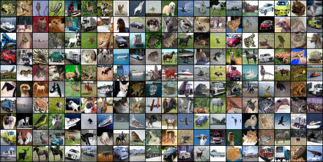
Figure 12: Generated samples from UOTM-SD (Linear) on CIFAR-10 ($32\times 32$).

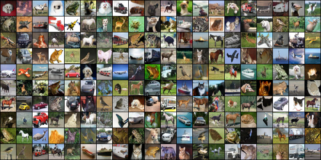
Figure 13: Generated samples from UOTM-SD (Step) on CIFAR-10 ($32\times 32$).

References

- Alvarez-Melis & Fusi (2020) David Alvarez-Melis and Nicolo Fusi. Geometric dataset distances via optimal transport. Advances in Neural Information Processing Systems, 33:21428–21439, 2020.
- An et al. (2019) Dongsheng An, Yang Guo, Na Lei, Zhongxuan Luo, Shing-Tung Yau, and Xianfeng Gu. Ae-ot: A new generative model based on extended semi-discrete optimal transport. ICLR 2020, 2019.
- An et al. (2020) Dongsheng An, Yang Guo, Min Zhang, Xin Qi, Na Lei, and Xianfang Gu. Ae-ot-gan: Training gans from data specific latent distribution. In Computer Vision–ECCV 2020: 16th European Conference, Glasgow, UK, August 23–28, 2020, Proceedings, Part XXVI 16, pp. 548–564. Springer, 2020.
- Ansari et al. (2020) Abdul Fatir Ansari, Ming Liang Ang, and Harold Soh. Refining deep generative models via discriminator gradient flow. arXiv preprint arXiv:2012.00780, 2020.
- Arjovsky et al. (2017) Martin Arjovsky, Soumith Chintala, and Léon Bottou. Wasserstein generative adversarial networks. In International conference on machine learning, pp. 214–223. PMLR, 2017.
- Balaji et al. (2020) Yogesh Balaji, Rama Chellappa, and Soheil Feizi. Robust optimal transport with applications in generative modeling and domain adaptation. Advances in Neural Information Processing Systems, 33:12934–12944, 2020.
- Chizat et al. (2018) Lenaic Chizat, Gabriel Peyré, Bernhard Schmitzer, and François-Xavier Vialard. Unbalanced optimal transport: Dynamic and kantorovich formulations. Journal of Functional Analysis, 274(11):3090–3123, 2018.
- Choi et al. (2023a) Jaemoo Choi, Jaewoong Choi, and Myungjoo Kang. Generative modeling through the semi-dual formulation of unbalanced optimal transport. arXiv preprint arXiv:2305.14777, 2023a.
- Choi et al. (2023b) Jaemoo Choi, Yesom Park, and Myungjoo Kang. Restoration based generative models. In Proceedings of the 40th International Conference on Machine Learning, volume 202. PMLR, 2023b.
- Csiszár (1972) Imre Csiszár. A class of measures of informativity of observation channels. Periodica Mathematica Hungarica, 2(1-4):191–213, 1972.
- Dockhorn et al. (2022) Tim Dockhorn, Arash Vahdat, and Karsten Kreis. Score-based generative modeling with critically-damped langevin diffusion. The International Conference on Learning Representations, 2022.
- (12) Jiaojiao Fan, Shu Liu, Shaojun Ma, Yongxin Chen, and Hao-Min Zhou. Scalable computation of monge maps with general costs. In ICLR Workshop on Deep Generative Models for Highly Structured Data.
- Fatras et al. (2021) Kilian Fatras, Thibault Séjourné, Rémi Flamary, and Nicolas Courty. Unbalanced minibatch optimal transport; applications to domain adaptation. In International Conference on Machine Learning, pp. 3186–3197. PMLR, 2021.
- Flamary et al. (2016) R Flamary, N Courty, D Tuia, and A Rakotomamonjy. Optimal transport for domain adaptation. IEEE Trans. Pattern Anal. Mach. Intell, 1, 2016.
- Gao et al. (2021) Ruiqi Gao, Yang Song, Ben Poole, Ying Nian Wu, and Diederik P Kingma. Learning energy-based models by diffusion recovery likelihood. Advances in neural information processing systems, 2021.
- Gong et al. (2019) Xinyu Gong, Shiyu Chang, Yifan Jiang, and Zhangyang Wang. Autogan: Neural architecture search for generative adversarial networks. In Proceedings of the IEEE/CVF International Conference on Computer Vision, pp. 3224–3234, 2019.
- Goodfellow et al. (2020) Ian Goodfellow, Jean Pouget-Abadie, Mehdi Mirza, Bing Xu, David Warde-Farley, Sherjil Ozair, Aaron Courville, and Yoshua Bengio. Generative adversarial networks. Communications of the ACM, 63(11):139–144, 2020.
- Guan et al. (2021) Hao Guan, Li Wang, and Mingxia Liu. Multi-source domain adaptation via optimal transport for brain dementia identification. In 2021 IEEE 18th International Symposium on Biomedical Imaging (ISBI), pp. 1514–1517. IEEE, 2021.
- Gulrajani et al. (2017) Ishaan Gulrajani, Faruk Ahmed, Martin Arjovsky, Vincent Dumoulin, and Aaron C Courville. Improved training of wasserstein gans. Advances in neural information processing systems, 30, 2017.
- He et al. (2016) Kaiming He, Xiangyu Zhang, Shaoqing Ren, and Jian Sun. Deep residual learning for image recognition. In Proceedings of the IEEE conference on computer vision and pattern recognition, pp. 770–778, 2016.
- Heusel et al. (2017) Martin Heusel, Hubert Ramsauer, Thomas Unterthiner, Bernhard Nessler, and Sepp Hochreiter. Gans trained by a two time-scale update rule converge to a local nash equilibrium. Advances in neural information processing systems, 30, 2017.
- Ho et al. (2020) Jonathan Ho, Ajay Jain, and Pieter Abbeel. Denoising diffusion probabilistic models. Advances in Neural Information Processing Systems, 33:6840–6851, 2020.
- Jiang et al. (2021) Yifan Jiang, Shiyu Chang, and Zhangyang Wang. Transgan: Two transformers can make one strong gan. arXiv preprint arXiv:2102.07074, 1(3), 2021.
- Jing et al. (2022) Bowen Jing, Gabriele Corso, Renato Berlinghieri, and Tommi Jaakkola. Subspace diffusion generative models. arXiv preprint arXiv:2205.01490, 2022.
- Kantorovich (1948) Leonid Vitalevich Kantorovich. On a problem of monge. Uspekhi Mat. Nauk, pp. 225–226, 1948.
- Karras et al. (2018) Tero Karras, Samuli Laine, and Timo Aila. A style-based generator architecture for generative adversarial networks. 2018.
- Karras et al. (2020) Tero Karras, Miika Aittala, Janne Hellsten, Samuli Laine, Jaakko Lehtinen, and Timo Aila. Training generative adversarial networks with limited data. Advances in Neural Information Processing Systems, 33:12104–12114, 2020.
- Khayatkhoei et al. (2018) Mahyar Khayatkhoei, Maneesh K Singh, and Ahmed Elgammal. Disconnected manifold learning for generative adversarial networks. Advances in Neural Information Processing Systems, 31, 2018.
- Kingma & Dhariwal (2018) Durk P Kingma and Prafulla Dhariwal. Glow: Generative flow with invertible 1x1 convolutions. Advances in neural information processing systems, 31, 2018.
- Korotin et al. (2022) Alexander Korotin, Daniil Selikhanovych, and Evgeny Burnaev. Neural optimal transport. arXiv preprint arXiv:2201.12220, 2022.
- Krizhevsky et al. (2009) Alex Krizhevsky, Geoffrey Hinton, et al. Learning multiple layers of features from tiny images. 2009.
- Liero et al. (2018) Matthias Liero, Alexander Mielke, and Giuseppe Savaré. Optimal entropy-transport problems and a new hellinger–kantorovich distance between positive measures. Inventiones mathematicae, 211(3):969–1117, 2018.
- Liu et al. (2019) Huidong Liu, Xianfeng Gu, and Dimitris Samaras. Wasserstein gan with quadratic transport cost. In Proceedings of the IEEE/CVF international conference on computer vision, pp. 4832–4841, 2019.
- Loshchilov & Hutter (2017) Ilya Loshchilov and Frank Hutter. SGDR: Stochastic gradient descent with warm restarts. In International Conference on Learning Representations, 2017. URL https://openreview.net/forum?id=Skq89Scxx.
- Makkuva et al. (2020) Ashok Makkuva, Amirhossein Taghvaei, Sewoong Oh, and Jason Lee. Optimal transport mapping via input convex neural networks. In International Conference on Machine Learning, pp. 6672–6681. PMLR, 2020.
- Mérigot et al. (2021) Quentin Mérigot, Filippo Santambrogio, and Clément Sarrazin. Non-asymptotic convergence bounds for wasserstein approximation using point clouds. Advances in Neural Information Processing Systems, 34:12810–12821, 2021.
- Mescheder et al. (2018) Lars Mescheder, Andreas Geiger, and Sebastian Nowozin. Which training methods for gans do actually converge? In International conference on machine learning, pp. 3481–3490. PMLR, 2018.
- (38) Takeru Miyato, Toshiki Kataoka, Masanori Koyama, and Yuichi Yoshida. Spectral normalization for generative adversarial networks. In International Conference on Learning Representations.
- Nagarajan & Kolter (2017) Vaishnavh Nagarajan and J Zico Kolter. Gradient descent gan optimization is locally stable. Advances in neural information processing systems, 30, 2017.
- Odena et al. (2018) Augustus Odena, Jacob Buckman, Catherine Olsson, Tom Brown, Christopher Olah, Colin Raffel, and Ian Goodfellow. Is generator conditioning causally related to gan performance? In International conference on machine learning, pp. 3849–3858. PMLR, 2018.
- Osborne & Rubinstein (1994) Martin J. Osborne and Ariel Rubinstein. A Course in Game Theory. The MIT Press, 1994. ISBN 0262150417.
- (42) Henning Petzka, Asja Fischer, and Denis Lukovnikov. On the regularization of wasserstein gans. In International Conference on Learning Representations.
- Peyré et al. (2017) Gabriel Peyré, Marco Cuturi, et al. Computational optimal transport. Center for Research in Economics and Statistics Working Papers, (2017-86), 2017.
- Radford et al. (2015) Alec Radford, Luke Metz, and Soumith Chintala. Unsupervised representation learning with deep convolutional generative adversarial networks. arXiv preprint arXiv:1511.06434, 2015.
- Roth et al. (2017) Kevin Roth, Aurelien Lucchi, Sebastian Nowozin, and Thomas Hofmann. Stabilizing training of generative adversarial networks through regularization. Advances in neural information processing systems, 30, 2017.
- (46) Litu Rout, Alexander Korotin, and Evgeny Burnaev. Generative modeling with optimal transport maps. In International Conference on Learning Representations.
- Salimans et al. (2016) Tim Salimans, Ian Goodfellow, Wojciech Zaremba, Vicki Cheung, Alec Radford, Xi Chen, and Xi Chen. Improved techniques for training gans. In D. Lee, M. Sugiyama, U. Luxburg, I. Guyon, and R. Garnett (eds.), Advances in Neural Information Processing Systems, volume 29, 2016.
- Salmona et al. (2022) Antoine Salmona, Valentin De Bortoli, Julie Delon, and Agnès Desolneux. Can push-forward generative models fit multimodal distributions? Advances in Neural Information Processing Systems, 35:10766–10779, 2022.
- Sanjabi et al. (2018) Maziar Sanjabi, Jimmy Ba, Meisam Razaviyayn, and Jason D Lee. On the convergence and robustness of training gans with regularized optimal transport. Advances in Neural Information Processing Systems, 31, 2018.
- Santambrogio (2015) Filippo Santambrogio. Optimal transport for applied mathematicians. Birkäuser, NY, 55(58-63):94, 2015.
- Sason & Verdú (2016) Igal Sason and Sergio Verdú. -divergence inequalities. IEEE Transactions on Information Theory, 62(11):5973–6006, 2016.
- Shen et al. (2018) Jian Shen, Yanru Qu, Weinan Zhang, and Yong Yu. Wasserstein distance guided representation learning for domain adaptation. In Proceedings of the AAAI Conference on Artificial Intelligence, volume 32, 2018.
- Song et al. (2021a) Jiaming Song, Chenlin Meng, and Stefano Ermon. Denoising diffusion implicit models. Advances in Neural Information Processing Systems, 2021a.
- Song & Ermon (2019) Yang Song and Stefano Ermon. Generative modeling by estimating gradients of the data distribution. Advances in Neural Information Processing Systems, 32, 2019.
- Song et al. (2021b) Yang Song, Jascha Sohl-Dickstein, Diederik P Kingma, Abhishek Kumar, Stefano Ermon, and Ben Poole. Score-based generative modeling through stochastic differential equations. The International Conference on Learning Representations, 2021b.
- Vahdat & Kautz (2020) Arash Vahdat and Jan Kautz. Nvae: A deep hierarchical variational autoencoder. Advances in Neural Information Processing Systems, 33:19667–19679, 2020.
- Vahdat et al. (2021) Arash Vahdat, Karsten Kreis, and Jan Kautz. Score-based generative modeling in latent space. Advances in Neural Information Processing Systems, 34:11287–11302, 2021.
- Van Oord et al. (2016) Aaron Van Oord, Nal Kalchbrenner, and Koray Kavukcuoglu. Pixel recurrent neural networks. In International conference on machine learning, pp. 1747–1756. PMLR, 2016.
- Villani et al. (2009) Cédric Villani et al. Optimal transport: old and new, volume 338. Springer, 2009.
- Xiao et al. (2020) Zhisheng Xiao, Karsten Kreis, Jan Kautz, and Arash Vahdat. Vaebm: A symbiosis between variational autoencoders and energy-based models. arXiv preprint arXiv:2010.00654, 2020.
- Xiao et al. (2021) Zhisheng Xiao, Karsten Kreis, and Arash Vahdat. Tackling the generative learning trilemma with denoising diffusion gans. arXiv preprint arXiv:2112.07804, 2021.
- Xie et al. (2019) Yujia Xie, Minshuo Chen, Haoming Jiang, Tuo Zhao, and Hongyuan Zha. On scalable and efficient computation of large scale optimal transport. volume 97 of proceedings of machine learning research. Long Beach, California, USA, pp. 09–15, 2019.
- Yang & Uhler (2019) KD Yang and C Uhler. Scalable unbalanced optimal transport using generative adversarial networks. In International Conference on Learning Representations, 2019.