Neural Bayes Estimators for Irregular Spatial Data using Graph Neural Networks

Abstract

Neural Bayes estimators are neural networks that approximate Bayes estimators in a fast and likelihood-free manner. They are appealing to use with spatial models and data, where estimation is often a computational bottleneck. However, neural Bayes estimators in spatial applications have, to date, been restricted to data collected over a regular grid. These estimators are also currently dependent on a prescribed set of spatial locations, which means that the neural network needs to be re-trained for new data sets; this renders them impractical in many applications and impedes their widespread adoption. In this work, we employ graph neural networks to tackle the important problem of parameter estimation from data collected over arbitrary spatial locations. In addition to extending neural Bayes estimation to irregular spatial data, our architecture leads to substantial computational benefits, since the estimator can be used with any arrangement or number of locations and independent replicates, thus amortising the cost of training for a given spatial model. We also facilitate fast uncertainty quantification by training an accompanying neural Bayes estimator that approximates a set of marginal posterior quantiles. We illustrate our methodology on Gaussian and max-stable processes. Finally, we showcase our methodology in a global sea-surface temperature application, where we estimate the parameters of a Gaussian process model in 2,161 regions, each containing thousands of irregularly-spaced data points, in just a few minutes with a single graphics processing unit.

Keywords: amortised inference, deep learning, extreme-value model, likelihood-free inference, neural network, spatial statistics

1 Introduction

The computational bottleneck when working with parametric statistical models often lies in making inference on the parameters. Neural Bayes estimators, that is, neural networks that approximate Bayes estimators, are being increasingly used for fast likelihood-free parameter inference (for an accessible introduction, see Sainsbury-Dale et al.,, 2023). In addition to being approximately Bayes and, therefore, statistically efficient, they are also amortised in the sense that, although the computational time and effort needed to initially train the underlying neural network can be substantial, once trained, inference from observed data that conform with the chosen neural-network architecture is extremely fast. These traits have seen neural Bayes estimators receiving attention from the fields of population genetics (Flagel et al.,, 2018), time series (Rudi et al.,, 2021), spatial statistics (Gerber and Nychka,, 2021; Banesh et al.,, 2021; Lenzi et al.,, 2023; Sainsbury-Dale et al.,, 2023), and spatio-temporal statistics (Zammit-Mangion and Wikle,, 2020). They have also been extended to accommodate settings in which some data are treated as censored, for example, when fitting certain classes of peaks-over-threshold dependence models for spatial extremes (Richards et al.,, 2023). Despite their promise and growing popularity, neural Bayes estimators for spatial models have, to date, mostly been applied to data collected over a regular grid, as gridded data facilitate the use of efficient convolutional neural networks (CNNs; Goodfellow et al.,, 2016, Ch. 9).

The restriction to gridded data is a major limitation in practice. To cater for irregular spatial data, Gerber_Nychka_2021_NN_param_estimation propose passing the empirical variogram as input to a dense neural network (DNN), also known as a multi-layer perceptron (MLP). This approach presupposes that the variogram is a summary statistic that carries substantial information for estimation. However, the variogram is based on the second moment of the data only, and it is unlikely to be close to sufficient for complex non-Gaussian models; in these cases, the resulting neural estimator will likely not be statistically efficient. More generally, the approach suggested by Gerber_Nychka_2021_NN_param_estimation is one in a class of neural approaches that bases estimation on a set of “good” summary statistics (see also Creel_2017; Rai_2023); such an approach can be expected to work well only if (near) sufficient summary statistics are indeed available. In practice, finite-dimensional sufficient statistics are not always available and often difficult to construct. Alternatively, one could treat each spatial datum as an independent input to a DNN; however, ignoring spatial dependence when building a neural estimator typically leads to a loss of statistical efficiency (Rudi_2020_NN_parameter_estimation; Sainsbury-Dale_2022_neural_Bayes_estimators), and such an estimator is again designed for a prescribed set of spatial sample locations, so that the network needs to be re-trained every time the spatial locations change (i.e., for every new data set). Hence, neural Bayes estimation from irregular spatial data remains an open and important problem.

In this work, we develop amortised neural Bayes estimators for irregular spatial data. Our novel approach involves representing the data as a graph with edges weighted by spatial distance, and then employing graph neural networks (GNNs; Zhang_2019_GCN_review; Zhou_2020_GNN_review; Wu_2021_GNN_review). GNNs generalise the convolution operation in conventional CNNs to graphical data, and have recently been used for regression problems in spatial statistics by, for example, Tonks_2022_GNNs_geostats, Zhan_Datta_2023_GNNs_geostats, and Cisneros_2023_GNNs_Australian_wildfire. Since they explicitly account for spatial dependence, GNNs provide a parsimonious representation for constructing neural Bayes estimators for irregular spatial data. Further, they can be used with data collected over any set of spatial locations; this means that GNN-based neural Bayes estimators only need to be trained once for a given spatial model. In addition to proposing the use of GNNs in this setting, we also consider several important practical issues: in particular, we show how to design a suitable architecture to perform inference both from a single spatial field and from replicates of a spatial process; how to construct synthetic spatial data sets for training such an estimator; and how to perform rigorous uncertainty quantification in an amortised manner, by training a neural Bayes estimator that approximates marginal posterior quantiles in a way that respects their ordering. Finally, to facilitate the use of GNN-based neural Bayes estimators by practitioners, we incorporate our methodology in the user-friendly software package NeuralEstimators (Sainsbury-Dale_2022_neural_Bayes_estimators), which is available in the Julia and R programming languages.

The remainder of this paper is organised as follows. In Section 2, we describe neural Bayes estimation for irregular spatial data using GNNs. In Section 3, we illustrate the strengths of the proposed approach by way of extensive simulation studies based on Gaussian and max-stable processes. In Section 4, we apply our methodology to the analysis of a massive global sea-surface temperature data set. In Section 5, we conclude and outline avenues for future research. A supplement is also available that contains additional details and figures. Code that reproduces all results in the manuscript is available from https://github.com/msainsburydale/NeuralEstimatorsGNN.

2 Methodology

In Section 2.1, we briefly review neural Bayes estimators; we refer readers to Sainsbury-Dale_2022_neural_Bayes_estimators for a more detailed discussion. In Section 2.2, we describe how GNNs may be used to perform neural Bayes inference for irregular spatial data.

2.1 Neural Bayes estimators

The goal of parameter point estimation is to estimate unknown model parameters ${\mathchoice{\hbox{\boldmath$\displaystyle{\theta}$}}{\hbox{\boldmath$\textstyle{\theta}$}}{\hbox{\boldmath$\scriptstyle{\theta}$}}{\hbox{\boldmath$\scriptscriptstyle{\theta}$}}}\in\Theta$ from data ${\mathchoice{\hbox{\boldmath$\displaystyle{Z}$}}{\hbox{\boldmath$\textstyle{Z}$}}{\hbox{\boldmath$\scriptstyle{Z}$}}{\hbox{\boldmath$\scriptscriptstyle{Z}$}}}\in\mathcal{S}$ using an estimator, $\hat{{\mathchoice{\hbox{\boldmath$\displaystyle{\theta}$}}{\hbox{\boldmath$\textstyle{\theta}$}}{\hbox{\boldmath$\scriptstyle{\theta}$}}{\hbox{\boldmath$\scriptscriptstyle{\theta}$}}}}\mathrel{\mathop{\mathchar 58\relax}}\mathcal{S}\to\Theta$, where $\mathcal{S}$ is the sample space and $\Theta$ is the parameter space. One typically seeks an estimator that performs well “on average” over all of $\mathcal{S}$ and $\Theta$, and such estimators can be constructed intuitively within a decision-theoretic framework. Consider a non-negative loss function, $L({\mathchoice{\hbox{\boldmath$\displaystyle{\theta}$}}{\hbox{\boldmath$\textstyle{\theta}$}}{\hbox{\boldmath$\scriptstyle{\theta}$}}{\hbox{\boldmath$\scriptscriptstyle{\theta}$}}},\hat{{\mathchoice{\hbox{\boldmath$\displaystyle{\theta}$}}{\hbox{\boldmath$\textstyle{\theta}$}}{\hbox{\boldmath$\scriptstyle{\theta}$}}{\hbox{\boldmath$\scriptscriptstyle{\theta}$}}}}({\mathchoice{\hbox{\boldmath$\displaystyle{Z}$}}{\hbox{\boldmath$\textstyle{Z}$}}{\hbox{\boldmath$\scriptstyle{Z}$}}{\hbox{\boldmath$\scriptscriptstyle{Z}$}}}))$, which assesses an estimator $\hat{{\mathchoice{\hbox{\boldmath$\displaystyle{\theta}$}}{\hbox{\boldmath$\textstyle{\theta}$}}{\hbox{\boldmath$\scriptstyle{\theta}$}}{\hbox{\boldmath$\scriptscriptstyle{\theta}$}}}}(\cdot)$ for a given $\textstyle{\theta}$ and realisation ${\mathchoice{\hbox{\boldmath$\displaystyle{Z}$}}{\hbox{\boldmath$\textstyle{Z}$}}{\hbox{\boldmath$\scriptstyle{Z}$}}{\hbox{\boldmath$\scriptscriptstyle{Z}$}}}\sim f({\mathchoice{\hbox{\boldmath$\displaystyle{z}$}}{\hbox{\boldmath$\textstyle{z}$}}{\hbox{\boldmath$\scriptstyle{z}$}}{\hbox{\boldmath$\scriptscriptstyle{z}$}}}\mid{\mathchoice{\hbox{\boldmath$\displaystyle{\theta}$}}{\hbox{\boldmath$\textstyle{\theta}$}}{\hbox{\boldmath$\scriptstyle{\theta}$}}{\hbox{\boldmath$\scriptscriptstyle{\theta}$}}})$, where $f({\mathchoice{\hbox{\boldmath$\displaystyle{z}$}}{\hbox{\boldmath$\textstyle{z}$}}{\hbox{\boldmath$\scriptstyle{z}$}}{\hbox{\boldmath$\scriptscriptstyle{z}$}}}\mid{\mathchoice{\hbox{\boldmath$\displaystyle{\theta}$}}{\hbox{\boldmath$\textstyle{\theta}$}}{\hbox{\boldmath$\scriptstyle{\theta}$}}{\hbox{\boldmath$\scriptscriptstyle{\theta}$}}})$ is the probability density function of the data conditional on $\textstyle{\theta}$. An estimator’s Bayes risk is its loss averaged over all possible data realisations and parameters values, that is,

$$r_{\Omega}(\hat{{\mathchoice{\hbox{\boldmath$\displaystyle{\theta}$}}{\hbox{\boldmath$\textstyle{\theta}$}}{\hbox{\boldmath$\scriptstyle{\theta}$}}{\hbox{\boldmath$\scriptscriptstyle{\theta}$}}}}(\cdot))\equiv\int_{\Theta}\int_{\mathcal{S}}L({\mathchoice{\hbox{\boldmath$\displaystyle{\theta}$}}{\hbox{\boldmath$\textstyle{\theta}$}}{\hbox{\boldmath$\scriptstyle{\theta}$}}{\hbox{\boldmath$\scriptscriptstyle{\theta}$}}},\hat{{\mathchoice{\hbox{\boldmath$\displaystyle{\theta}$}}{\hbox{\boldmath$\textstyle{\theta}$}}{\hbox{\boldmath$\scriptstyle{\theta}$}}{\hbox{\boldmath$\scriptscriptstyle{\theta}$}}}}({\mathchoice{\hbox{\boldmath$\displaystyle{z}$}}{\hbox{\boldmath$\textstyle{z}$}}{\hbox{\boldmath$\scriptstyle{z}$}}{\hbox{\boldmath$\scriptscriptstyle{z}$}}}))f({\mathchoice{\hbox{\boldmath$\displaystyle{z}$}}{\hbox{\boldmath$\textstyle{z}$}}{\hbox{\boldmath$\scriptstyle{z}$}}{\hbox{\boldmath$\scriptscriptstyle{z}$}}}\mid{\mathchoice{\hbox{\boldmath$\displaystyle{\theta}$}}{\hbox{\boldmath$\textstyle{\theta}$}}{\hbox{\boldmath$\scriptstyle{\theta}$}}{\hbox{\boldmath$\scriptscriptstyle{\theta}$}}})\textrm{d}{\mathchoice{\hbox{\boldmath$\displaystyle{z}$}}{\hbox{\boldmath$\textstyle{z}$}}{\hbox{\boldmath$\scriptstyle{z}$}}{\hbox{\boldmath$\scriptscriptstyle{z}$}}}\textrm{d}\Omega({\mathchoice{\hbox{\boldmath$\displaystyle{\theta}$}}{\hbox{\boldmath$\textstyle{\theta}$}}{\hbox{\boldmath$\scriptstyle{\theta}$}}{\hbox{\boldmath$\scriptscriptstyle{\theta}$}}}),$$ (1)

where $\Omega(\cdot)$ is a prior measure for $\textstyle{\theta}$. A minimiser of (1) is said to be a Bayes estimator with respect to $L(\cdot,\cdot)$ and $\Omega(\cdot)$.

Bayes estimators are theoretically attractive, being consistent and asymptotically efficient under mild conditions (Lehmann_Casella_1998_Point_Estimation, Thm. 5.2.4; Thm. 6.8.3). Unfortunately, however, Bayes estimators are typically unavailable in closed form. Recently, neural networks have been used to approximate Bayes estimators, motivated by universal function approximation theorems (e.g., Hornik_1989_FNN_universal_approximation_theorem; Zhou_2018_universal_approximation_CNNs) and the speed at which they can be evaluated. Let $\hat{{\mathchoice{\hbox{\boldmath$\displaystyle{\theta}$}}{\hbox{\boldmath$\textstyle{\theta}$}}{\hbox{\boldmath$\scriptstyle{\theta}$}}{\hbox{\boldmath$\scriptscriptstyle{\theta}$}}}}(\cdot;{\mathchoice{\hbox{\boldmath$\displaystyle{\gamma}$}}{\hbox{\boldmath$\textstyle{\gamma}$}}{\hbox{\boldmath$\scriptstyle{\gamma}$}}{\hbox{\boldmath$\scriptscriptstyle{\gamma}$}}})$ denote a neural network that returns a point estimate from data $\textstyle{Z}$, with $\textstyle{\gamma}$ comprising the neural-network parameters. Bayes estimators may be approximated with $\hat{{\mathchoice{\hbox{\boldmath$\displaystyle{\theta}$}}{\hbox{\boldmath$\textstyle{\theta}$}}{\hbox{\boldmath$\scriptstyle{\theta}$}}{\hbox{\boldmath$\scriptscriptstyle{\theta}$}}}}(\cdot;{\mathchoice{\hbox{\boldmath$\displaystyle{\gamma}$}}{\hbox{\boldmath$\textstyle{\gamma}$}}{\hbox{\boldmath$\scriptstyle{\gamma}$}}{\hbox{\boldmath$\scriptscriptstyle{\gamma}$}}}^{*})$, where ${\mathchoice{\hbox{\boldmath$\displaystyle{\gamma}$}}{\hbox{\boldmath$\textstyle{\gamma}$}}{\hbox{\boldmath$\scriptstyle{\gamma}$}}{\hbox{\boldmath$\scriptscriptstyle{\gamma}$}}}^{*}$ solves the optimisation task

$${\mathchoice{\hbox{\boldmath$\displaystyle{\gamma}$}}{\hbox{\boldmath$\textstyle{\gamma}$}}{\hbox{\boldmath$\scriptstyle{\gamma}$}}{\hbox{\boldmath$\scriptscriptstyle{\gamma}$}}}^{*}\equiv\underset{{\mathchoice{\hbox{\boldmath$\displaystyle{\gamma}$}}{\hbox{\boldmath$\textstyle{\gamma}$}}{\hbox{\boldmath$\scriptstyle{\gamma}$}}{\hbox{\boldmath$\scriptscriptstyle{\gamma}$}}}}{\mathrm{arg\,min}}\;\frac{1}{K}\sum_{{\mathchoice{\hbox{\boldmath$\displaystyle{\theta}$}}{\hbox{\boldmath$\textstyle{\theta}$}}{\hbox{\boldmath$\scriptstyle{\theta}$}}{\hbox{\boldmath$\scriptscriptstyle{\theta}$}}}\in\vartheta}\frac{1}{J}\sum_{{\mathchoice{\hbox{\boldmath$\displaystyle{Z}$}}{\hbox{\boldmath$\textstyle{Z}$}}{\hbox{\boldmath$\scriptstyle{Z}$}}{\hbox{\boldmath$\scriptscriptstyle{Z}$}}}\in\mathcal{Z}_{{\mathchoice{\hbox{\boldmath$\displaystyle{\theta}$}}{\hbox{\boldmath$\textstyle{\theta}$}}{\hbox{\boldmath$\scriptstyle{\theta}$}}{\hbox{\boldmath$\scriptscriptstyle{\theta}$}}}}}L({\mathchoice{\hbox{\boldmath$\displaystyle{\theta}$}}{\hbox{\boldmath$\textstyle{\theta}$}}{\hbox{\boldmath$\scriptstyle{\theta}$}}{\hbox{\boldmath$\scriptscriptstyle{\theta}$}}},\hat{{\mathchoice{\hbox{\boldmath$\displaystyle{\theta}$}}{\hbox{\boldmath$\textstyle{\theta}$}}{\hbox{\boldmath$\scriptstyle{\theta}$}}{\hbox{\boldmath$\scriptscriptstyle{\theta}$}}}}({\mathchoice{\hbox{\boldmath$\displaystyle{Z}$}}{\hbox{\boldmath$\textstyle{Z}$}}{\hbox{\boldmath$\scriptstyle{Z}$}}{\hbox{\boldmath$\scriptscriptstyle{Z}$}}};{\mathchoice{\hbox{\boldmath$\displaystyle{\gamma}$}}{\hbox{\boldmath$\textstyle{\gamma}$}}{\hbox{\boldmath$\scriptstyle{\gamma}$}}{\hbox{\boldmath$\scriptscriptstyle{\gamma}$}}})),$$ (2)

whose objective function is a Monte Carlo approximation of (1) made using a set $\vartheta$ of $K$ parameter vectors sampled from the prior $\Omega(\cdot)$ and, for each ${\mathchoice{\hbox{\boldmath$\displaystyle{\theta}$}}{\hbox{\boldmath$\textstyle{\theta}$}}{\hbox{\boldmath$\scriptstyle{\theta}$}}{\hbox{\boldmath$\scriptscriptstyle{\theta}$}}}\in\vartheta$, a set $\mathcal{Z}_{{\mathchoice{\hbox{\boldmath$\displaystyle{\theta}$}}{\hbox{\boldmath$\textstyle{\theta}$}}{\hbox{\boldmath$\scriptstyle{\theta}$}}{\hbox{\boldmath$\scriptscriptstyle{\theta}$}}}}$ of $J$ realisations from $f({\mathchoice{\hbox{\boldmath$\displaystyle{z}$}}{\hbox{\boldmath$\textstyle{z}$}}{\hbox{\boldmath$\scriptstyle{z}$}}{\hbox{\boldmath$\scriptscriptstyle{z}$}}}\mid{\mathchoice{\hbox{\boldmath$\displaystyle{\theta}$}}{\hbox{\boldmath$\textstyle{\theta}$}}{\hbox{\boldmath$\scriptstyle{\theta}$}}{\hbox{\boldmath$\scriptscriptstyle{\theta}$}}})$. The optimisation task (2) is a form of empirical risk minimisation (Goodfellow_2016_Deep_learning, pg. 268–269), and it can be solved efficiently using back-propagation and stochastic gradient descent; moreover, it does not involve evaluation, or knowledge, of the likelihood function. The fitted neural network approximately minimises the Bayes risk, and is thus called a neural Bayes estimator.

Neural Bayes estimators, like all neural networks, are function approximators that, under mild conditions, can theoretically approximate continuous functions arbitrarily well. There is a need for more theory in this emerging field to determine the conditions needed for a trained neural Bayes estimator to be within an $\epsilon$-ball from the true Bayes estimator with high probability: conditions on the size of the network in terms of its width and depth, and the number of training samples, that is, $J$ and $K$ in (2), would be particularly helpful in guiding practitioners. While such theoretical developments are important, they are beyond the scope of this paper. Nevertheless, due to their speed, it is straightforward to empirically assess the performance of a trained neural Bayes estimator; by applying the estimator to many simulated data sets, one can quickly and accurately assess a trained estimator with respect to any property of its sampling distribution.

As discussed in Section 1, neural Bayes estimators for spatial data have, to date, mostly been limited to data collected over a grid, in which case CNNs may be employed. DNNs can in principle be used for irregular data, but they do not explicitly account for spatial dependence and they are conditional on a single set of spatial locations. Constructing an estimator based on user-defined summary statistics is an appealing option, but it is only possible when easy-to-compute near-sufficient summary statistics are available. We therefore seek an architecture that parsimoniously models spatial dependence; that is able to yield a statistically efficient estimator by automatically constructing near-sufficient statistics from the full data set; and that can be applied to data collected over arbitrary spatial locations. The next subsection describes how this can be achieved.

2.2 Neural Bayes estimators for irregular spatial data

In Section 2.2.1, we describe how GNNs may be used in a novel way to construct neural Bayes estimators for irregular spatial data, where inference is made from a single field. In Section 2.2.2, we describe how to account for varying spatial configurations. In Section 2.2.3, we describe how GNNs may be used to estimate parameters from independent replicates of a spatial process. In Section 2.2.4, we discuss the important task of uncertainty quantification.

2.2.1 Inference from a single spatial field

GNNs are a broad class of neural networks designed for graphical data, and they have been the subject of recent reviews by Zhang_2019_GCN_review, Zhou_2020_GNN_review, and Wu_2021_GNN_review. GNNs generalise the convolution operation in conventional CNNs and, therefore, they are able to efficiently extract information about the dependence structure in graphical data. GNNs can also generalise to different graphical inputs (of potentially different sizes, connections, edge weights, etc.), and they can scale well with the graph size, particularly for sparse graphs. These key properties make GNNs natural candidates for constructing neural Bayes estimators for irregular spatial data, where the spatial data are viewed as a (sparse) graph with edges weighted by spatial distance. In what follows, we assume that we have data ${\mathchoice{\hbox{\boldmath$\displaystyle{Z}$}}{\hbox{\boldmath$\textstyle{Z}$}}{\hbox{\boldmath$\scriptstyle{Z}$}}{\hbox{\boldmath$\scriptscriptstyle{Z}$}}}\equiv(Z_{1},\dots,Z_{n})^{\prime}$ observed at spatial locations $\{{\mathchoice{\hbox{\boldmath$\displaystyle{s}$}}{\hbox{\boldmath$\textstyle{s}$}}{\hbox{\boldmath$\scriptstyle{s}$}}{\hbox{\boldmath$\scriptscriptstyle{s}$}}}_{1},\dots,{\mathchoice{\hbox{\boldmath$\displaystyle{s}$}}{\hbox{\boldmath$\textstyle{s}$}}{\hbox{\boldmath$\scriptstyle{s}$}}{\hbox{\boldmath$\scriptscriptstyle{s}$}}}_{n}\}\in\mathcal{D}$, where $\mathcal{D}$ is the spatial domain of interest. We collect the spatial locations in the matrix ${\mathchoice{\hbox{\boldmath$\displaystyle{S}$}}{\hbox{\boldmath$\textstyle{S}$}}{\hbox{\boldmath$\scriptstyle{S}$}}{\hbox{\boldmath$\scriptscriptstyle{S}$}}}\equiv({\mathchoice{\hbox{\boldmath$\displaystyle{s}$}}{\hbox{\boldmath$\textstyle{s}$}}{\hbox{\boldmath$\scriptstyle{s}$}}{\hbox{\boldmath$\scriptscriptstyle{s}$}}}_{1},\dots,{\mathchoice{\hbox{\boldmath$\displaystyle{s}$}}{\hbox{\boldmath$\textstyle{s}$}}{\hbox{\boldmath$\scriptstyle{s}$}}{\hbox{\boldmath$\scriptscriptstyle{s}$}}}_{n})^{\prime}$.

In the context of deep learning, parameter estimation from irregular spatial data constitutes a “graph-level regression task”, where the entire graph (spatial data) is associated with some fixed-dimensional vector (model parameters) that we wish to estimate. The architecture of a typical GNN used for graph-level regression and, hence, the architecture for our GNN-based neural Bayes estimator, consists of three modules that are applied sequentially: the propagation module, the readout module, and the mapping module. Figure 1 shows a pedagogical example.

Figure 1: The architecture of our proposed GNN-based neural Bayes estimator for a single spatial field. The spatial data, ${\mathchoice{\hbox{\boldmath$\displaystyle{Z}$}}{\hbox{\boldmath$\textstyle{Z}$}}{\hbox{\boldmath$\scriptstyle{Z}$}}{\hbox{\boldmath$\scriptscriptstyle{Z}$}}}=(Z_{1},\dots,Z_{n})^{\prime}$, here shown for $n=4$ locations, ${\mathchoice{\hbox{\boldmath$\displaystyle{S}$}}{\hbox{\boldmath$\textstyle{S}$}}{\hbox{\boldmath$\scriptstyle{S}$}}{\hbox{\boldmath$\scriptscriptstyle{S}$}}}=({\mathchoice{\hbox{\boldmath$\displaystyle{s}$}}{\hbox{\boldmath$\textstyle{s}$}}{\hbox{\boldmath$\scriptstyle{s}$}}{\hbox{\boldmath$\scriptscriptstyle{s}$}}}_{1},\dots,{\mathchoice{\hbox{\boldmath$\displaystyle{s}$}}{\hbox{\boldmath$\textstyle{s}$}}{\hbox{\boldmath$\scriptstyle{s}$}}{\hbox{\boldmath$\scriptscriptstyle{s}$}}}_{n})^{\prime}$, are sequentially convolved by the Ł -layered propagation module into a graph with hidden-feature vectors $\{{\mathchoice{\hbox{\boldmath$\displaystyle{h}$}}{\hbox{\boldmath$\textstyle{h}$}}{\hbox{\boldmath$\scriptstyle{h}$}}{\hbox{\boldmath$\scriptscriptstyle{h}$}}}^{(\mathchoice{\scalebox{1.0}{\L}}{\scalebox{0.95}{\L}}{\scalebox{0.7}{\L}}{\scalebox{0.5}{\L}})}_{1},\dots,{\mathchoice{\hbox{\boldmath$\displaystyle{h}$}}{\hbox{\boldmath$\textstyle{h}$}}{\hbox{\boldmath$\scriptstyle{h}$}}{\hbox{\boldmath$\scriptscriptstyle{h}$}}}^{(\mathchoice{\scalebox{1.0}{\L}}{\scalebox{0.95}{\L}}{\scalebox{0.7}{\L}}{\scalebox{0.5}{\L}})}_{n}\}$. Pairs of nodes are determined to be neighbours or not based on spatial proximity, $d_{jj^{\prime}}=\|{\mathchoice{\hbox{\boldmath$\displaystyle{s}$}}{\hbox{\boldmath$\textstyle{s}$}}{\hbox{\boldmath$\scriptstyle{s}$}}{\hbox{\boldmath$\scriptscriptstyle{s}$}}}_{j^{\prime}}-{\mathchoice{\hbox{\boldmath$\displaystyle{s}$}}{\hbox{\boldmath$\textstyle{s}$}}{\hbox{\boldmath$\scriptstyle{s}$}}{\hbox{\boldmath$\scriptscriptstyle{s}$}}}_{j}\|$, $j,j^{\prime}\in\{1,\dots,n\}$. The readout module summarises this graph into a vector of summary statistics, $\textstyle{R}$, that is fixed in length (here of length five) irrespective of the size of the input graph. Finally, the mapping module transforms $\textstyle{R}$ into parameter estimates, $\hat{{\mathchoice{\hbox{\boldmath$\displaystyle{\theta}$}}{\hbox{\boldmath$\textstyle{\theta}$}}{\hbox{\boldmath$\scriptstyle{\theta}$}}{\hbox{\boldmath$\scriptscriptstyle{\theta}$}}}}=(\hat{\theta}_{1},\dots,\hat{\theta}_{p})^{\prime}$, here shown for $p=3$, where the non-linear mapping is done using a DNN.

In the propagation module, a graph-convolution operator is applied to each node to form a series of hidden feature graphs, which have the same size and structure as the input graph (unless the graph-coarsening technique known as “local pooling” is applied between propagation layers; see Mesquita_2020_pooling; Grattarola_2022_pooling). A large class of propagation modules can be couched in the so-called “message-passing” framework (Gilmer_2017_message_passing_GNNs), where spatial-based convolutions are performed locally on each node (i.e., graph vertex) and its neighbours. Note that information is passed between non-neighbouring nodes by applying local convolutions in successive layers, thereby allowing global relationships to be modelled. This approach scales well with the graph size, since only a subset of nodes are considered for each computation, and it allows a single GNN to generalise to different graph structures, since the convolutional parameters are shared across the graph. In our spatial setting, we define the propagation module as

$${\mathchoice{\hbox{\boldmath$\displaystyle{h}$}}{\hbox{\boldmath$\textstyle{h}$}}{\hbox{\boldmath$\scriptstyle{h}$}}{\hbox{\boldmath$\scriptscriptstyle{h}$}}}^{(l)}_{j}=g\Big{(}{\mathchoice{\hbox{\boldmath$\displaystyle{\Gamma}$}}{\hbox{\boldmath$\textstyle{\Gamma}$}}{\hbox{\boldmath$\scriptstyle{\Gamma}$}}{\hbox{\boldmath$\scriptscriptstyle{\Gamma}$}}}_{\!1}^{(l)}{\mathchoice{\hbox{\boldmath$\displaystyle{h}$}}{\hbox{\boldmath$\textstyle{h}$}}{\hbox{\boldmath$\scriptstyle{h}$}}{\hbox{\boldmath$\scriptscriptstyle{h}$}}}^{(l-1)}_{j}+\frac{1}{|\mathcal{N}(j)|}\sum_{j^{\prime}\in\mathcal{N}(j)}\exp\Big{(}\frac{-d_{jj^{\prime}}}{\gamma^{(l)}}\Big{)}{\mathchoice{\hbox{\boldmath$\displaystyle{\Gamma}$}}{\hbox{\boldmath$\textstyle{\Gamma}$}}{\hbox{\boldmath$\scriptstyle{\Gamma}$}}{\hbox{\boldmath$\scriptscriptstyle{\Gamma}$}}}_{\!2}^{(l)}{\mathchoice{\hbox{\boldmath$\displaystyle{h}$}}{\hbox{\boldmath$\textstyle{h}$}}{\hbox{\boldmath$\scriptstyle{h}$}}{\hbox{\boldmath$\scriptscriptstyle{h}$}}}^{(l-1)}_{j^{\prime}}\Big{)},\quad l=1,\dots,\mathchoice{\scalebox{1.0}{\L}}{\scalebox{0.95}{\L}}{\scalebox{0.7}{\L}}{\scalebox{0.5}{\L}},$$ (3)

where, for $j=1,\dots,n$, ${\mathchoice{\hbox{\boldmath$\displaystyle{h}$}}{\hbox{\boldmath$\textstyle{h}$}}{\hbox{\boldmath$\scriptstyle{h}$}}{\hbox{\boldmath$\scriptscriptstyle{h}$}}}^{(l)}_{j}$ is the hidden-feature vector at location ${\mathchoice{\hbox{\boldmath$\displaystyle{s}$}}{\hbox{\boldmath$\textstyle{s}$}}{\hbox{\boldmath$\scriptstyle{s}$}}{\hbox{\boldmath$\scriptscriptstyle{s}$}}}_{j}$ at layer $l$, ${\mathchoice{\hbox{\boldmath$\displaystyle{h}$}}{\hbox{\boldmath$\textstyle{h}$}}{\hbox{\boldmath$\scriptstyle{h}$}}{\hbox{\boldmath$\scriptscriptstyle{h}$}}}_{j}^{(0)}=Z_{j}$ (the datum at ${\mathchoice{\hbox{\boldmath$\displaystyle{s}$}}{\hbox{\boldmath$\textstyle{s}$}}{\hbox{\boldmath$\scriptstyle{s}$}}{\hbox{\boldmath$\scriptscriptstyle{s}$}}}_{j}$), $g(\cdot)$ is a non-linear activation function applied elementwise, ${\mathchoice{\hbox{\boldmath$\displaystyle{\Gamma}$}}{\hbox{\boldmath$\textstyle{\Gamma}$}}{\hbox{\boldmath$\scriptstyle{\Gamma}$}}{\hbox{\boldmath$\scriptscriptstyle{\Gamma}$}}}_{\!1}^{(l)}$ and ${\mathchoice{\hbox{\boldmath$\displaystyle{\Gamma}$}}{\hbox{\boldmath$\textstyle{\Gamma}$}}{\hbox{\boldmath$\scriptstyle{\Gamma}$}}{\hbox{\boldmath$\scriptscriptstyle{\Gamma}$}}}_{\!2}^{(l)}$ are trainable parameter matrices for the $l$th layer, $\mathcal{N}(j)$ denotes the indices of neighbours of ${\mathchoice{\hbox{\boldmath$\displaystyle{s}$}}{\hbox{\boldmath$\textstyle{s}$}}{\hbox{\boldmath$\scriptstyle{s}$}}{\hbox{\boldmath$\scriptscriptstyle{s}$}}}_{j}$, $d_{jj^{\prime}}=\|{\mathchoice{\hbox{\boldmath$\displaystyle{s}$}}{\hbox{\boldmath$\textstyle{s}$}}{\hbox{\boldmath$\scriptstyle{s}$}}{\hbox{\boldmath$\scriptscriptstyle{s}$}}}_{j^{\prime}}-{\mathchoice{\hbox{\boldmath$\displaystyle{s}$}}{\hbox{\boldmath$\textstyle{s}$}}{\hbox{\boldmath$\scriptstyle{s}$}}{\hbox{\boldmath$\scriptscriptstyle{s}$}}}_{j}\|$ denotes a distance (typically Euclidean) between ${\mathchoice{\hbox{\boldmath$\displaystyle{s}$}}{\hbox{\boldmath$\textstyle{s}$}}{\hbox{\boldmath$\scriptstyle{s}$}}{\hbox{\boldmath$\scriptscriptstyle{s}$}}}_{j}$ and ${\mathchoice{\hbox{\boldmath$\displaystyle{s}$}}{\hbox{\boldmath$\textstyle{s}$}}{\hbox{\boldmath$\scriptstyle{s}$}}{\hbox{\boldmath$\scriptscriptstyle{s}$}}}_{j^{\prime}}$ for $j^{\prime}\in\mathcal{N}(j)$, $\gamma^{(l)}>0$ is a trainable range parameter for the $l$th layer, and Ł is the total number of layers. We construct the neighbourhoods based on spatial proximity. Specifically, we consider pairs of nodes to be neighbours if their spatial distance is below a pre-specified threshold (up to a maximum number of neighbours); we discuss this further in Section 2.2.2. Although other propagation modules are possible, (3) is a flexible one that can capture complex spatial relationships, and we adopt it throughout this work.

In the readout module, the graph output from the propagation module is aggregated into a vector of summary statistics, $\textstyle{R}$, which is fixed in length irrespective of the size and structure of the input graph. We express this readout module as

$${\mathchoice{\hbox{\boldmath$\displaystyle{R}$}}{\hbox{\boldmath$\textstyle{R}$}}{\hbox{\boldmath$\scriptstyle{R}$}}{\hbox{\boldmath$\scriptscriptstyle{R}$}}}={\mathchoice{\hbox{\boldmath$\displaystyle{r}$}}{\hbox{\boldmath$\textstyle{r}$}}{\hbox{\boldmath$\scriptstyle{r}$}}{\hbox{\boldmath$\scriptscriptstyle{r}$}}}(\{{\mathchoice{\hbox{\boldmath$\displaystyle{h}$}}{\hbox{\boldmath$\textstyle{h}$}}{\hbox{\boldmath$\scriptstyle{h}$}}{\hbox{\boldmath$\scriptscriptstyle{h}$}}}^{(\mathchoice{\scalebox{1.0}{\L}}{\scalebox{0.95}{\L}}{\scalebox{0.7}{\L}}{\scalebox{0.5}{\L}})}_{j}\mathrel{\mathop{\mathchar 58\relax}}j=1,\dots,n\}),$$ (4)

where the readout function, ${\mathchoice{\hbox{\boldmath$\displaystyle{r}$}}{\hbox{\boldmath$\textstyle{r}$}}{\hbox{\boldmath$\scriptstyle{r}$}}{\hbox{\boldmath$\scriptscriptstyle{r}$}}}(\{\cdot\})$, is a permutation-invariant set function, and recall that $n$ denotes the number of observed spatial locations. Each element of ${\mathchoice{\hbox{\boldmath$\displaystyle{r}$}}{\hbox{\boldmath$\textstyle{r}$}}{\hbox{\boldmath$\scriptstyle{r}$}}{\hbox{\boldmath$\scriptscriptstyle{r}$}}}(\{\cdot\})$ is typically chosen to be a simple aggregation function (e.g., elementwise addition, average, maximum, or other quantiles), but more flexible, parameterised readout modules have also been proposed in the context of general graph-level regression (e.g., Navarin_2019_universal_readout). In this paper, we use the elementwise average. For many statistical models used in practice, the number of summary statistics in $\textstyle{R}$ required to reach (near) sufficiency for $\textstyle{\theta}$ is unknown and, in these cases, the length of $\textstyle{R}$ should be chosen to be reasonably large. In this work, we set the length of $\textstyle{R}$ to be 128. The readout module allows a GNN to be applied to arbitrary graph structures and, therefore, allows a single GNN-based neural Bayes estimator to make inference from data collected over any number and arrangement of spatial locations.

Finally, the mapping module maps the vector of fixed-length summary statistics, $\textstyle{R}$, into parameter estimates,

$$\hat{{\mathchoice{\hbox{\boldmath$\displaystyle{\theta}$}}{\hbox{\boldmath$\textstyle{\theta}$}}{\hbox{\boldmath$\scriptstyle{\theta}$}}{\hbox{\boldmath$\scriptscriptstyle{\theta}$}}}}={\mathchoice{\hbox{\boldmath$\displaystyle{\xi}$}}{\hbox{\boldmath$\textstyle{\xi}$}}{\hbox{\boldmath$\scriptstyle{\xi}$}}{\hbox{\boldmath$\scriptscriptstyle{\xi}$}}}({\mathchoice{\hbox{\boldmath$\displaystyle{R}$}}{\hbox{\boldmath$\textstyle{R}$}}{\hbox{\boldmath$\scriptstyle{R}$}}{\hbox{\boldmath$\scriptscriptstyle{R}$}}};{\mathchoice{\hbox{\boldmath$\displaystyle{\gamma}$}}{\hbox{\boldmath$\textstyle{\gamma}$}}{\hbox{\boldmath$\scriptstyle{\gamma}$}}{\hbox{\boldmath$\scriptscriptstyle{\gamma}$}}}_{\xi}),$$ (5)

where ${\mathchoice{\hbox{\boldmath$\displaystyle{\xi}$}}{\hbox{\boldmath$\textstyle{\xi}$}}{\hbox{\boldmath$\scriptstyle{\xi}$}}{\hbox{\boldmath$\scriptscriptstyle{\xi}$}}}(\cdot;{\mathchoice{\hbox{\boldmath$\displaystyle{\gamma}$}}{\hbox{\boldmath$\textstyle{\gamma}$}}{\hbox{\boldmath$\scriptstyle{\gamma}$}}{\hbox{\boldmath$\scriptscriptstyle{\gamma}$}}}_{\xi})$ is a DNN parameterised by ${\mathchoice{\hbox{\boldmath$\displaystyle{\gamma}$}}{\hbox{\boldmath$\textstyle{\gamma}$}}{\hbox{\boldmath$\scriptstyle{\gamma}$}}{\hbox{\boldmath$\scriptscriptstyle{\gamma}$}}}_{\xi}$. Our estimator can thus be viewed as a non-linear mapping of the summary statistics extracted in $\textstyle{R}$, which are themselves non-linear mappings of the data $\textstyle{Z}$ and spatial locations $\textstyle{S}$.

2.2.2 Training the estimator to account for varying spatial locations

Note from (3)–(5) that a GNN-based neural Bayes estimator is a function of the spatial locations of the data, and that it can be applied to data collected over any number and configuration of spatial locations. If one wishes to make inference from a single spatial data set only, and this data set is collected before the estimator is constructed, then data for the optimisation task (2) can be simulated using the observed spatial locations, which can be treated as fixed and known. However, if one wishes to construct an estimator that is approximately Bayes for a large range of spatial configurations (and number of spatial locations), then one requires an estimator $\hat{{\mathchoice{\hbox{\boldmath$\displaystyle{\theta}$}}{\hbox{\boldmath$\textstyle{\theta}$}}{\hbox{\boldmath$\scriptstyle{\theta}$}}{\hbox{\boldmath$\scriptscriptstyle{\theta}$}}}}(\cdot;{\mathchoice{\hbox{\boldmath$\displaystyle{S}$}}{\hbox{\boldmath$\textstyle{S}$}}{\hbox{\boldmath$\scriptstyle{S}$}}{\hbox{\boldmath$\scriptscriptstyle{S}$}}})$ that conditions on the observed spatial locations ${\mathchoice{\hbox{\boldmath$\displaystyle{S}$}}{\hbox{\boldmath$\textstyle{S}$}}{\hbox{\boldmath$\scriptstyle{S}$}}{\hbox{\boldmath$\scriptscriptstyle{S}$}}}=({\mathchoice{\hbox{\boldmath$\displaystyle{s}$}}{\hbox{\boldmath$\textstyle{s}$}}{\hbox{\boldmath$\scriptstyle{s}$}}{\hbox{\boldmath$\scriptscriptstyle{s}$}}}_{1},\dots,{\mathchoice{\hbox{\boldmath$\displaystyle{s}$}}{\hbox{\boldmath$\textstyle{s}$}}{\hbox{\boldmath$\scriptstyle{s}$}}{\hbox{\boldmath$\scriptscriptstyle{s}$}}}_{n})^{\prime}$, with $\textstyle{S}$ (and $n$) treated as random. Then, assuming that $\textstyle{S}$ is independent of both the data and the parameters, the Bayes risk (1) becomes

$$r_{\Omega}(\hat{{\mathchoice{\hbox{\boldmath$\displaystyle{\theta}$}}{\hbox{\boldmath$\textstyle{\theta}$}}{\hbox{\boldmath$\scriptstyle{\theta}$}}{\hbox{\boldmath$\scriptscriptstyle{\theta}$}}}}(\cdot;\cdot))\equiv\int_{\mathcal{G}}\int_{\Theta}\int_{\mathcal{S}}L({\mathchoice{\hbox{\boldmath$\displaystyle{\theta}$}}{\hbox{\boldmath$\textstyle{\theta}$}}{\hbox{\boldmath$\scriptstyle{\theta}$}}{\hbox{\boldmath$\scriptscriptstyle{\theta}$}}},\hat{{\mathchoice{\hbox{\boldmath$\displaystyle{\theta}$}}{\hbox{\boldmath$\textstyle{\theta}$}}{\hbox{\boldmath$\scriptstyle{\theta}$}}{\hbox{\boldmath$\scriptscriptstyle{\theta}$}}}}({\mathchoice{\hbox{\boldmath$\displaystyle{z}$}}{\hbox{\boldmath$\textstyle{z}$}}{\hbox{\boldmath$\scriptstyle{z}$}}{\hbox{\boldmath$\scriptscriptstyle{z}$}}};{\mathchoice{\hbox{\boldmath$\displaystyle{S}$}}{\hbox{\boldmath$\textstyle{S}$}}{\hbox{\boldmath$\scriptstyle{S}$}}{\hbox{\boldmath$\scriptscriptstyle{S}$}}}))f({\mathchoice{\hbox{\boldmath$\displaystyle{z}$}}{\hbox{\boldmath$\textstyle{z}$}}{\hbox{\boldmath$\scriptstyle{z}$}}{\hbox{\boldmath$\scriptscriptstyle{z}$}}}\mid{\mathchoice{\hbox{\boldmath$\displaystyle{\theta}$}}{\hbox{\boldmath$\textstyle{\theta}$}}{\hbox{\boldmath$\scriptstyle{\theta}$}}{\hbox{\boldmath$\scriptscriptstyle{\theta}$}}})\textrm{d}{\mathchoice{\hbox{\boldmath$\displaystyle{z}$}}{\hbox{\boldmath$\textstyle{z}$}}{\hbox{\boldmath$\scriptstyle{z}$}}{\hbox{\boldmath$\scriptscriptstyle{z}$}}}\textrm{d}\Omega({\mathchoice{\hbox{\boldmath$\displaystyle{\theta}$}}{\hbox{\boldmath$\textstyle{\theta}$}}{\hbox{\boldmath$\scriptstyle{\theta}$}}{\hbox{\boldmath$\scriptscriptstyle{\theta}$}}})\textrm{d}\Pi({\mathchoice{\hbox{\boldmath$\displaystyle{S}$}}{\hbox{\boldmath$\textstyle{S}$}}{\hbox{\boldmath$\scriptstyle{S}$}}{\hbox{\boldmath$\scriptscriptstyle{S}$}}}),$$ (6)

where $\mathcal{G}$ is the space of all possible spatial configurations, and $\Pi(\cdot)$ is a prior measure for $\textstyle{S}$. Note that, the number of spatial locations, $n$, is a random quantity whose prior measure is implicitly defined by the measure $\Pi(\cdot)$. A minimiser of (6) is a Bayes estimator with respect to $L(\cdot,\cdot)$, $\Omega(\cdot)$, and $\Pi(\cdot)$.

If no prior knowledge on the spatial configuration is available, then a reasonably uninformative prior measure for $\textstyle{S}$ should be used to produce an estimator that is broadly applicable. Spatial point-process models (Moller_2004_point_patterns; Illian_2008_point_patterns; Diggle_2013_point_patterns) are ideal for this purpose. A convenient point-process model to generate a wide range of spatial configurations is the Matérn cluster process (Baddeley_2015_point_patterns, Ch. 12). Simulation of $\textstyle{S}$ from a Matérn cluster process proceeds by first simulating from a homogeneous Poisson point process with intensity $\lambda>0$ and then, for each point in this underlying (unobserved) point process, simulating a Poisson number of points with mean $\mu>0$ uniformly on a disk with constant radius $\delta>0$. Figure 2 shows realisations from a Matérn cluster process under several parameter choices. In practice, the parameters $\lambda$, $\mu$, and $\delta$ may be selected by visualising realisations from the cluster process (as done in Figure 2) and modifying the parameters until the sampled spatial configurations cover a sufficiently wide range of scenarios (e.g., from sparse to dense, and from highly clustered to approximately uniform). There are many other point-process models that could be used (e.g., log-Gaussian Cox processes); the specific model used is unlikely to meaningfully affect the final estimator, provided that the model is able to generate a wide range of plausible spatial configurations. In Section 3, we show that training with different sampling configurations allows a GNN-based neural Bayes estimator to be approximately Bayes irrespective of the locations the data.

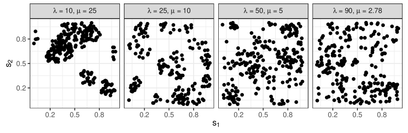
Figure 2: Realisations from a Matérn cluster process with parent Poisson point process intensity $\lambda$, mean number of daughter points $\mu$, and cluster-disk radius $\delta=0.1$. Various parameter combinations (see panel titles) were here chosen such that the expected number of sampled points, $\lambda\mu$, is fixed to 250. Spatial point processes are useful when constructing training data in order to cover a wide range of spatial configurations.

The definition of the neighbourhood in (3) is important, particularly when the number of observed locations, $n$, may vary. One possibility is to define the neighbourhood of a node as its $k$-nearest spatial neighbours with some fixed $k$, which results in an estimator with a computational complexity of $\mathcal{O}(n)$; however, with a fixed bounded domain, the spatial proximity of the $k$-nearest neighbours depends on $n$, which can compromise the estimator’s ability to extrapolate to more locations than used during training, since the estimator is calibrated for a certain distribution of the distances between a node and its neighbours. To mitigate this issue, one may define the neighbourhood of a given node as a disc of fixed radius. This definition makes the estimator more robust to different spatial configurations, since the distribution of the distances between a node and its neighbours no longer depends on $n$ and, in the case of small $n$ or highly unbalanced spatial configurations, distant nodes are not treated as neighbours. However, for a fixed spatial domain, this fixed-radius definition results in a computational complexity of $\mathcal{O}(n^{2})$, since increasing $n$ simultaneously increases the total number of nodes that must be convolved, and the number of neighbours for existing nodes. Therefore, we combine these two methods by (randomly) selecting $k$ nodes within a node’s neighbourhood disc. This definition harnesses the benefits of both methods, namely, it results in an estimator that has a computational complexity of $\mathcal{O}(n)$, as well as one which is stable with respect to the size of the data set. Note that randomness in the neighbourhood set leads to variability in the resulting estimator; if deemed an issue, this variability can be removed by using a deterministic selection strategy, such as one based on a minimum-maximum ordering, as is often employed in Vecchia approximations to likelihood functions (Guinness_2018).

2.2.3 Inference with independent replicates

Inference is often made from multiple independent replicates of a spatial field, particularly when modelling spatial extremes, or when working with highly-parameterised or weakly-identifiable models. In this case, we have multiple graphs (of potentially different structures) associated with a single output, which is not a standard problem in the GNN literature. We address this challenge by couching GNNs within the DeepSets framework (Zaheer_2017_Deep_Sets), which was also employed in the context of neural Bayes estimation for gridded spatial data by Sainsbury-Dale_2022_neural_Bayes_estimators. Suppose that we have data from $m$ mutually independent realisations from a spatial process that we collect in ${\mathchoice{\hbox{\boldmath$\displaystyle{Z}$}}{\hbox{\boldmath$\textstyle{Z}$}}{\hbox{\boldmath$\scriptstyle{Z}$}}{\hbox{\boldmath$\scriptscriptstyle{Z}$}}}\equiv({\mathchoice{\hbox{\boldmath$\displaystyle{Z}$}}{\hbox{\boldmath$\textstyle{Z}$}}{\hbox{\boldmath$\scriptstyle{Z}$}}{\hbox{\boldmath$\scriptscriptstyle{Z}$}}}_{1}^{\prime},\dots,{\mathchoice{\hbox{\boldmath$\displaystyle{Z}$}}{\hbox{\boldmath$\textstyle{Z}$}}{\hbox{\boldmath$\scriptstyle{Z}$}}{\hbox{\boldmath$\scriptscriptstyle{Z}$}}}_{m}^{\prime})^{\prime}$, where the locations, ${\mathchoice{\hbox{\boldmath$\displaystyle{S}$}}{\hbox{\boldmath$\textstyle{S}$}}{\hbox{\boldmath$\scriptstyle{S}$}}{\hbox{\boldmath$\scriptscriptstyle{S}$}}}_{i}\equiv({\mathchoice{\hbox{\boldmath$\displaystyle{s}$}}{\hbox{\boldmath$\textstyle{s}$}}{\hbox{\boldmath$\scriptstyle{s}$}}{\hbox{\boldmath$\scriptscriptstyle{s}$}}}_{i1},\dots,{\mathchoice{\hbox{\boldmath$\displaystyle{s}$}}{\hbox{\boldmath$\textstyle{s}$}}{\hbox{\boldmath$\scriptstyle{s}$}}{\hbox{\boldmath$\scriptscriptstyle{s}$}}}_{in_{i}})^{\prime}$, and number of observations, $n_{i}$, are allowed to vary between realisations $i=1,\dots,m$. Then, DeepSets-based parameter estimates may be evaluated from the data $\textstyle{Z}$ and their spatial locations as

$$\hat{{\mathchoice{\hbox{\boldmath$\displaystyle{\theta}$}}{\hbox{\boldmath$\textstyle{\theta}$}}{\hbox{\boldmath$\scriptstyle{\theta}$}}{\hbox{\boldmath$\scriptscriptstyle{\theta}$}}}} ={\mathchoice{\hbox{\boldmath$\displaystyle{\phi}$}}{\hbox{\boldmath$\textstyle{\phi}$}}{\hbox{\boldmath$\scriptstyle{\phi}$}}{\hbox{\boldmath$\scriptscriptstyle{\phi}$}}}({\mathchoice{\hbox{\boldmath$\displaystyle{T}$}}{\hbox{\boldmath$\textstyle{T}$}}{\hbox{\boldmath$\scriptstyle{T}$}}{\hbox{\boldmath$\scriptscriptstyle{T}$}}};{\mathchoice{\hbox{\boldmath$\displaystyle{\gamma}$}}{\hbox{\boldmath$\textstyle{\gamma}$}}{\hbox{\boldmath$\scriptstyle{\gamma}$}}{\hbox{\boldmath$\scriptscriptstyle{\gamma}$}}}_{\phi}),$$ (7)

$${\mathchoice{\hbox{\boldmath$\displaystyle{T}$}}{\hbox{\boldmath$\textstyle{T}$}}{\hbox{\boldmath$\scriptstyle{T}$}}{\hbox{\boldmath$\scriptscriptstyle{T}$}}} ={\mathchoice{\hbox{\boldmath$\displaystyle{a}$}}{\hbox{\boldmath$\textstyle{a}$}}{\hbox{\boldmath$\scriptstyle{a}$}}{\hbox{\boldmath$\scriptscriptstyle{a}$}}}\big{(}\{{\mathchoice{\hbox{\boldmath$\displaystyle{R}$}}{\hbox{\boldmath$\textstyle{R}$}}{\hbox{\boldmath$\scriptstyle{R}$}}{\hbox{\boldmath$\scriptscriptstyle{R}$}}}_{i}\mathrel{\mathop{\mathchar 58\relax}}i=1,\dots,m\}\big{)},$$

$${\mathchoice{\hbox{\boldmath$\displaystyle{R}$}}{\hbox{\boldmath$\textstyle{R}$}}{\hbox{\boldmath$\scriptstyle{R}$}}{\hbox{\boldmath$\scriptscriptstyle{R}$}}}_{i} ={\mathchoice{\hbox{\boldmath$\displaystyle{\psi}$}}{\hbox{\boldmath$\textstyle{\psi}$}}{\hbox{\boldmath$\scriptstyle{\psi}$}}{\hbox{\boldmath$\scriptscriptstyle{\psi}$}}}(\{{\mathchoice{\hbox{\boldmath$\displaystyle{Z}$}}{\hbox{\boldmath$\textstyle{Z}$}}{\hbox{\boldmath$\scriptstyle{Z}$}}{\hbox{\boldmath$\scriptscriptstyle{Z}$}}}_{i},{\mathchoice{\hbox{\boldmath$\displaystyle{S}$}}{\hbox{\boldmath$\textstyle{S}$}}{\hbox{\boldmath$\scriptstyle{S}$}}{\hbox{\boldmath$\scriptscriptstyle{S}$}}}_{i}\};{\mathchoice{\hbox{\boldmath$\displaystyle{\gamma}$}}{\hbox{\boldmath$\textstyle{\gamma}$}}{\hbox{\boldmath$\scriptstyle{\gamma}$}}{\hbox{\boldmath$\scriptscriptstyle{\gamma}$}}}_{\psi}),\quad i=1,\dots,m,$$

where ${\mathchoice{\hbox{\boldmath$\displaystyle{\psi}$}}{\hbox{\boldmath$\textstyle{\psi}$}}{\hbox{\boldmath$\scriptstyle{\psi}$}}{\hbox{\boldmath$\scriptscriptstyle{\psi}$}}}(\cdot;{\mathchoice{\hbox{\boldmath$\displaystyle{\gamma}$}}{\hbox{\boldmath$\textstyle{\gamma}$}}{\hbox{\boldmath$\scriptstyle{\gamma}$}}{\hbox{\boldmath$\scriptscriptstyle{\gamma}$}}}_{\psi})$ corresponds to the composition of the propagation and readout modules of a standard GNN with parameters ${\mathchoice{\hbox{\boldmath$\displaystyle{\gamma}$}}{\hbox{\boldmath$\textstyle{\gamma}$}}{\hbox{\boldmath$\scriptstyle{\gamma}$}}{\hbox{\boldmath$\scriptscriptstyle{\gamma}$}}}_{\psi}$ corresponding to the neural-network parameters in (3), ${\mathchoice{\hbox{\boldmath$\displaystyle{R}$}}{\hbox{\boldmath$\textstyle{R}$}}{\hbox{\boldmath$\scriptstyle{R}$}}{\hbox{\boldmath$\scriptscriptstyle{R}$}}}_{i}$ is a vector summarising ${\mathchoice{\hbox{\boldmath$\displaystyle{Z}$}}{\hbox{\boldmath$\textstyle{Z}$}}{\hbox{\boldmath$\scriptstyle{Z}$}}{\hbox{\boldmath$\scriptscriptstyle{Z}$}}}_{i}$ that is fixed in length irrespective of $i$, ${\mathchoice{\hbox{\boldmath$\displaystyle{a}$}}{\hbox{\boldmath$\textstyle{a}$}}{\hbox{\boldmath$\scriptstyle{a}$}}{\hbox{\boldmath$\scriptscriptstyle{a}$}}}(\{\cdot\})$ is a permutation-invariant set function (here chosen to be the elementwise average), $\textstyle{T}$ is a fixed-length vector summarising $\textstyle{Z}$, and ${\mathchoice{\hbox{\boldmath$\displaystyle{\phi}$}}{\hbox{\boldmath$\textstyle{\phi}$}}{\hbox{\boldmath$\scriptstyle{\phi}$}}{\hbox{\boldmath$\scriptscriptstyle{\phi}$}}}(\cdot;{\mathchoice{\hbox{\boldmath$\displaystyle{\gamma}$}}{\hbox{\boldmath$\textstyle{\gamma}$}}{\hbox{\boldmath$\scriptstyle{\gamma}$}}{\hbox{\boldmath$\scriptscriptstyle{\gamma}$}}}_{\phi})$ is a DNN parameterised by ${\mathchoice{\hbox{\boldmath$\displaystyle{\gamma}$}}{\hbox{\boldmath$\textstyle{\gamma}$}}{\hbox{\boldmath$\scriptstyle{\gamma}$}}{\hbox{\boldmath$\scriptscriptstyle{\gamma}$}}}_{\phi}$. Figure 3 illustrates the architecture (7). Note that, when applied to a single replicate (i.e., when $m=1$), (7) reduces to the architecture proposed in Section 2.2.1.

The representation (7) has several motivations. First, Bayes estimators are invariant to permutations of independent replicates; estimators constructed from (7) are guaranteed to exhibit this property. Further, functions of the form (7) can approximate any continuously differentiable permutation-invariant function arbitrarily well (Wagstaff_2021_universal_approximation_set_functions; Han_2019_universal_approximation_of_symmetric_functions); therefore, an estimator constructed in the form (7) can theoretically approximate any Bayes estimator that is a continuously differentiable function of the data. Finally, (7) may be applied to data sets with an arbitrary number of replicates, $m$, which allows the training cost to be amortised with respect to the number of replicates. See Sainsbury-Dale_2022_neural_Bayes_estimators for further details on the use of the DeepSets architecture in the context of neural Bayes estimation, and for a discussion on the architecture’s connection to conventional estimators.

Figure 3: The structure of a GNN-based neural Bayes estimator when making inference from $m$ mutually independent realisations, ${\mathchoice{\hbox{\boldmath$\displaystyle{Z}$}}{\hbox{\boldmath$\textstyle{Z}$}}{\hbox{\boldmath$\scriptstyle{Z}$}}{\hbox{\boldmath$\scriptscriptstyle{Z}$}}}_{1},\dots,{\mathchoice{\hbox{\boldmath$\displaystyle{Z}$}}{\hbox{\boldmath$\textstyle{Z}$}}{\hbox{\boldmath$\scriptstyle{Z}$}}{\hbox{\boldmath$\scriptscriptstyle{Z}$}}}_{m}$, observed at spatial locations, ${\mathchoice{\hbox{\boldmath$\displaystyle{S}$}}{\hbox{\boldmath$\textstyle{S}$}}{\hbox{\boldmath$\scriptstyle{S}$}}{\hbox{\boldmath$\scriptscriptstyle{S}$}}}_{1},\dots,{\mathchoice{\hbox{\boldmath$\displaystyle{S}$}}{\hbox{\boldmath$\textstyle{S}$}}{\hbox{\boldmath$\scriptstyle{S}$}}{\hbox{\boldmath$\scriptscriptstyle{S}$}}}_{m}$. The realisations are processed independently by ${\mathchoice{\hbox{\boldmath$\displaystyle{\psi}$}}{\hbox{\boldmath$\textstyle{\psi}$}}{\hbox{\boldmath$\scriptstyle{\psi}$}}{\hbox{\boldmath$\scriptscriptstyle{\psi}$}}}(\cdot)$, which is the composition of the propagation and readout modules described in Section 2.2.1, into a set of fixed-length vectors, ${\mathchoice{\hbox{\boldmath$\displaystyle{R}$}}{\hbox{\boldmath$\textstyle{R}$}}{\hbox{\boldmath$\scriptstyle{R}$}}{\hbox{\boldmath$\scriptscriptstyle{R}$}}}_{1},\dots,{\mathchoice{\hbox{\boldmath$\displaystyle{R}$}}{\hbox{\boldmath$\textstyle{R}$}}{\hbox{\boldmath$\scriptstyle{R}$}}{\hbox{\boldmath$\scriptscriptstyle{R}$}}}_{m}$. These vectors are aggregated using a permutation-invariant set function, ${\mathchoice{\hbox{\boldmath$\displaystyle{a}$}}{\hbox{\boldmath$\textstyle{a}$}}{\hbox{\boldmath$\scriptstyle{a}$}}{\hbox{\boldmath$\scriptscriptstyle{a}$}}}(\cdot)$, into a single vector of summary statistics, $\textstyle{T}$, which is then transformed by a DNN ${\mathchoice{\hbox{\boldmath$\displaystyle{\phi}$}}{\hbox{\boldmath$\textstyle{\phi}$}}{\hbox{\boldmath$\scriptstyle{\phi}$}}{\hbox{\boldmath$\scriptscriptstyle{\phi}$}}}(\cdot)$ into parameter estimates $\hat{{\mathchoice{\hbox{\boldmath$\displaystyle{\theta}$}}{\hbox{\boldmath$\textstyle{\theta}$}}{\hbox{\boldmath$\scriptstyle{\theta}$}}{\hbox{\boldmath$\scriptscriptstyle{\theta}$}}}}$.

2.2.4 Uncertainty quantification

Uncertainty quantification with neural Bayes estimators often proceeds through the bootstrap distribution (e.g., Lenzi_2021_NN_param_estimation; Sainsbury-Dale_2022_neural_Bayes_estimators; Richards_2023_censoring). Bootstrap-based approaches are particularly attractive when non-parametric bootstrap is possible (e.g., when the data are replicated), or when simulation from the fitted model is fast, in which case parametric bootstrap is also computationally efficient. However, these conditions are not always met in spatial statistics. For example, when making inference from a single spatial field, non-parametric bootstrap is not possible without breaking the spatial dependence structure, and the cost of simulation from the fitted model is often non-negligible (e.g., exact simulation from a Gaussian process model requires the factorisation of an $n\times n$ matrix, where $n$ is the number of spatial locations, which is a task that is $\mathcal{O}(n^{3})$ in computational complexity).

Alternatively, one may construct a neural Bayes estimator that approximates a set of marginal posterior quantiles, which can then be used to construct credible intervals. Inference then remains fully amortised since, once the neural Bayes estimators are trained, both point estimates and credible intervals can be obtained at almost no computational cost. Posterior quantiles can be targeted by employing the quantile loss function (e.g., Cressie_2022_loss_functions, Eqn. 7) which, for a single parameter $\theta$, is given by

$$\tilde{L}_{q}(\theta,\hat{\theta})=(\hat{\theta}-\theta)(\mathbb{I}(\hat{\theta}>\theta)-q),\quad q\in(0,1),$$ (8)

where $\mathbb{I}(\cdot)$ denotes the indicator function. In particular, the Bayes estimator under (8) is the $q$th posterior quantile. When there are $p>1$ parameters, ${\mathchoice{\hbox{\boldmath$\displaystyle{\theta}$}}{\hbox{\boldmath$\textstyle{\theta}$}}{\hbox{\boldmath$\scriptstyle{\theta}$}}{\hbox{\boldmath$\scriptscriptstyle{\theta}$}}}=(\theta_{1},\dots,\theta_{p})^{\prime}$, we define the joint loss function by summing (8) over each parameter, ${L({\mathchoice{\hbox{\boldmath$\displaystyle{\theta}$}}{\hbox{\boldmath$\textstyle{\theta}$}}{\hbox{\boldmath$\scriptstyle{\theta}$}}{\hbox{\boldmath$\scriptscriptstyle{\theta}$}}},\hat{{\mathchoice{\hbox{\boldmath$\displaystyle{\theta}$}}{\hbox{\boldmath$\textstyle{\theta}$}}{\hbox{\boldmath$\scriptstyle{\theta}$}}{\hbox{\boldmath$\scriptscriptstyle{\theta}$}}}})=\sum_{k=1}^{p}\tilde{L}_{q}(\theta_{k},\hat{\theta}_{k})}$. The Bayes estimator under this joint loss function is the vector of marginal posterior quantiles since, in general, a Bayes estimator under a sum of univariate loss functions is given by the vector of marginal Bayes estimators (see Theorem 1 in Appendix A).

Consider, for ease of exposition, the case where neural Bayes estimators are just a function of the data $\textstyle{Z}$. To ensure the correct ordering of the output quantiles, we design our neural Bayes estimator to map the data $\textstyle{Z}$ into intervals of the form

$$[U_{k}({\mathchoice{\hbox{\boldmath$\displaystyle{Z}$}}{\hbox{\boldmath$\textstyle{Z}$}}{\hbox{\boldmath$\scriptstyle{Z}$}}{\hbox{\boldmath$\scriptscriptstyle{Z}$}}}),U_{k}({\mathchoice{\hbox{\boldmath$\displaystyle{Z}$}}{\hbox{\boldmath$\textstyle{Z}$}}{\hbox{\boldmath$\scriptstyle{Z}$}}{\hbox{\boldmath$\scriptscriptstyle{Z}$}}})+\mathrm{exp}(V_{k}({\mathchoice{\hbox{\boldmath$\displaystyle{Z}$}}{\hbox{\boldmath$\textstyle{Z}$}}{\hbox{\boldmath$\scriptstyle{Z}$}}{\hbox{\boldmath$\scriptscriptstyle{Z}$}}}))],\quad k=1,\dots,p,$$ (9)

where ${\mathchoice{\hbox{\boldmath$\displaystyle{U}$}}{\hbox{\boldmath$\textstyle{U}$}}{\hbox{\boldmath$\scriptstyle{U}$}}{\hbox{\boldmath$\scriptscriptstyle{U}$}}}(\cdot)\equiv(U_{1}(\cdot),\dots,U_{p}(\cdot))^{\prime}$ and ${\mathchoice{\hbox{\boldmath$\displaystyle{V}$}}{\hbox{\boldmath$\textstyle{V}$}}{\hbox{\boldmath$\scriptstyle{V}$}}{\hbox{\boldmath$\scriptscriptstyle{V}$}}}(\cdot)\equiv(V_{1}(\cdot),\dots,V_{p}(\cdot))^{\prime}$ are neural networks that transform data into $p$-dimensional vectors (these neural networks are parameterised, but we do not make this explicit for notational convenience). In our context of making inference from irregular spatial data, these neural networks have architectures of the form (5) when $\textstyle{Z}$ contains a single replicate, or (7) when $\textstyle{Z}$ contains multiple replicates. We optimise the neural-network parameters in ${\mathchoice{\hbox{\boldmath$\displaystyle{U}$}}{\hbox{\boldmath$\textstyle{U}$}}{\hbox{\boldmath$\scriptstyle{U}$}}{\hbox{\boldmath$\scriptscriptstyle{U}$}}}(\cdot)$ and ${\mathchoice{\hbox{\boldmath$\displaystyle{V}$}}{\hbox{\boldmath$\textstyle{V}$}}{\hbox{\boldmath$\scriptstyle{V}$}}{\hbox{\boldmath$\scriptscriptstyle{V}$}}}(\cdot)$ jointly. This is done by defining ${\mathchoice{\hbox{\boldmath$\displaystyle{Q}$}}{\hbox{\boldmath$\textstyle{Q}$}}{\hbox{\boldmath$\scriptstyle{Q}$}}{\hbox{\boldmath$\scriptscriptstyle{Q}$}}}(\cdot)\equiv(Q_{1}(\cdot),\dots,Q_{2p}(\cdot))^{\prime}=({\mathchoice{\hbox{\boldmath$\displaystyle{U}$}}{\hbox{\boldmath$\textstyle{U}$}}{\hbox{\boldmath$\scriptstyle{U}$}}{\hbox{\boldmath$\scriptscriptstyle{U}$}}}(\cdot)^{\prime},{\mathchoice{\hbox{\boldmath$\displaystyle{U}$}}{\hbox{\boldmath$\textstyle{U}$}}{\hbox{\boldmath$\scriptstyle{U}$}}{\hbox{\boldmath$\scriptscriptstyle{U}$}}}(\cdot)^{\prime}+\exp\!{({\mathchoice{\hbox{\boldmath$\displaystyle{V}$}}{\hbox{\boldmath$\textstyle{V}$}}{\hbox{\boldmath$\scriptstyle{V}$}}{\hbox{\boldmath$\scriptscriptstyle{V}$}}}(\cdot))^{\prime}})^{\prime}$, where the exponential function is applied elementwise, and performing the optimisation task (2) under the loss function,

$$\sum_{k=1}^{p}\tilde{L}_{q_{1}}(\theta_{k},Q_{k}({\mathchoice{\hbox{\boldmath$\displaystyle{Z}$}}{\hbox{\boldmath$\textstyle{Z}$}}{\hbox{\boldmath$\scriptstyle{Z}$}}{\hbox{\boldmath$\scriptscriptstyle{Z}$}}}))+\sum_{k=1}^{p}\tilde{L}_{q_{2}}(\theta_{k},Q_{k+p}({\mathchoice{\hbox{\boldmath$\displaystyle{Z}$}}{\hbox{\boldmath$\textstyle{Z}$}}{\hbox{\boldmath$\scriptstyle{Z}$}}{\hbox{\boldmath$\scriptscriptstyle{Z}$}}})),$$

where $q_{1}$ and $q_{2}>q_{1}$ are low and high probability levels, respectively. By Theorem 1, once the neural-network parameters in ${\mathchoice{\hbox{\boldmath$\displaystyle{Q}$}}{\hbox{\boldmath$\textstyle{Q}$}}{\hbox{\boldmath$\scriptstyle{Q}$}}{\hbox{\boldmath$\scriptscriptstyle{Q}$}}}(\cdot)$ have been optimised, the first $p$ outputs of ${\mathchoice{\hbox{\boldmath$\displaystyle{Q}$}}{\hbox{\boldmath$\textstyle{Q}$}}{\hbox{\boldmath$\scriptstyle{Q}$}}{\hbox{\boldmath$\scriptscriptstyle{Q}$}}}(\cdot)$ approximate the marginal posterior $q_{1}$-quantiles, and the second $p$ outputs of ${\mathchoice{\hbox{\boldmath$\displaystyle{Q}$}}{\hbox{\boldmath$\textstyle{Q}$}}{\hbox{\boldmath$\scriptstyle{Q}$}}{\hbox{\boldmath$\scriptscriptstyle{Q}$}}}(\cdot)$ approximate the marginal posterior $q_{2}$-quantiles.

Finally, we note that there are several extensions of (9) that may be useful in some settings. First, one could extend (9) to jointly approximate the marginal posterior median (for point estimation) and other marginal posterior quantiles (for uncertainty quantification) in such a way that the point estimator is always contained within the corresponding credible interval. Second, when the marginal prior distribution for each parameter has compact support, ${\textrm{supp}(\theta_{k})}$, $k=1,\dots,p$, it is possible to modify (9) to ensure that the intervals are contained within the prior support. With this modification, our neural Bayes estimator maps data $\textstyle{Z}$ into intervals of the form

$$[g_{k}(U_{k}({\mathchoice{\hbox{\boldmath$\displaystyle{Z}$}}{\hbox{\boldmath$\textstyle{Z}$}}{\hbox{\boldmath$\scriptstyle{Z}$}}{\hbox{\boldmath$\scriptscriptstyle{Z}$}}})),g_{k}(U_{k}({\mathchoice{\hbox{\boldmath$\displaystyle{Z}$}}{\hbox{\boldmath$\textstyle{Z}$}}{\hbox{\boldmath$\scriptstyle{Z}$}}{\hbox{\boldmath$\scriptscriptstyle{Z}$}}})+\mathrm{exp}(V_{k}({\mathchoice{\hbox{\boldmath$\displaystyle{Z}$}}{\hbox{\boldmath$\textstyle{Z}$}}{\hbox{\boldmath$\scriptstyle{Z}$}}{\hbox{\boldmath$\scriptscriptstyle{Z}$}}})))],\quad k=1,\dots,p,$$ (10)

where $g_{k}(\cdot)$ is a logistic function that maps the real line to ${\textrm{supp}(\theta_{k})}$. Since the logistic function is monotonic, the architecture (10) also ensures that the quantiles do not cross.

3 Simulation studies

We now conduct several simulation studies to demonstrate the efficacy of GNN-based neural Bayes estimators for estimating parameters in spatial models. In Section 3.1, we outline the general setting. In Section 3.2, we estimate the parameters of a Gaussian process model. Since the likelihood function is available for this model, we compare our GNN-based estimator to that of the gold-standard maximum-likelihood (ML) estimator. In Section 3.3, we consider a spatial extremes setting and estimate the two parameters of Schlather’s max-stable model (Schlather_2002_max-stable_models): the likelihood function is computationally intractable for this model, and we are able to obtain substantial improvements over the usual composite-likelihood approach that is often used with this model.

3.1 General setting

Across the simulation studies we take the spatial domain to be the unit square. We implement our neural Bayes estimators using functionality we have added to the package NeuralEstimators (Sainsbury-Dale_2022_neural_Bayes_estimators), which is available in both the Julia and R programming languages. The GNN functionality of the package employs the Julia package GraphNeuralNetworks (Lucibello2021GNN). We conduct our experiments using a workstation with an AMD EPYC 7402 3.00GHz CPU with 52 cores and 128 GB of CPU RAM, and a Nvidia Quadro RTX 6000 GPU with 24 GB of GPU RAM. All results presented in the remainder of this paper can be generated using the reproducible code available at https://github.com/msainsburydale/NeuralEstimatorsGNN.

Our GNN architecture, summarised in Table S1 of the supplementary material, is based on the representation (7) which, we recall, can be applied to an arbitrary number $m$ of independent spatial fields (including $m=1$). The inner network, ${\mathchoice{\hbox{\boldmath$\displaystyle{\psi}$}}{\hbox{\boldmath$\textstyle{\psi}$}}{\hbox{\boldmath$\scriptstyle{\psi}$}}{\hbox{\boldmath$\scriptscriptstyle{\psi}$}}}(\cdot;{\mathchoice{\hbox{\boldmath$\displaystyle{\gamma}$}}{\hbox{\boldmath$\textstyle{\gamma}$}}{\hbox{\boldmath$\scriptstyle{\gamma}$}}{\hbox{\boldmath$\scriptscriptstyle{\gamma}$}}}_{\psi})$, is the composition of the propagation and readout modules; we use a propagation module based on (3) with 4 layers and 128 channels in each layer (i.e., ${\mathchoice{\hbox{\boldmath$\displaystyle{\Gamma}$}}{\hbox{\boldmath$\textstyle{\Gamma}$}}{\hbox{\boldmath$\scriptstyle{\Gamma}$}}{\hbox{\boldmath$\scriptscriptstyle{\Gamma}$}}}_{\!1}^{(l)}$ and ${\mathchoice{\hbox{\boldmath$\displaystyle{\Gamma}$}}{\hbox{\boldmath$\textstyle{\Gamma}$}}{\hbox{\boldmath$\scriptstyle{\Gamma}$}}{\hbox{\boldmath$\scriptscriptstyle{\Gamma}$}}}_{\!2}^{(l)}$ in (3) each have 128 rows for $l=1,\dots,4$), and define the neighbours of a node as those points falling within 0.2 units from that node (and randomly select up to a maximum of $k=30$ neighbours). We use the elementwise average for each element of ${\mathchoice{\hbox{\boldmath$\displaystyle{r}$}}{\hbox{\boldmath$\textstyle{r}$}}{\hbox{\boldmath$\scriptstyle{r}$}}{\hbox{\boldmath$\scriptscriptstyle{r}$}}}(\{\cdot\})$ in (4) and each element of ${\mathchoice{\hbox{\boldmath$\displaystyle{a}$}}{\hbox{\boldmath$\textstyle{a}$}}{\hbox{\boldmath$\scriptstyle{a}$}}{\hbox{\boldmath$\scriptscriptstyle{a}$}}}(\{\cdot\})$ in (7). The outer neural network, ${\mathchoice{\hbox{\boldmath$\displaystyle{\phi}$}}{\hbox{\boldmath$\textstyle{\phi}$}}{\hbox{\boldmath$\scriptstyle{\phi}$}}{\hbox{\boldmath$\scriptscriptstyle{\phi}$}}}(\cdot;{\mathchoice{\hbox{\boldmath$\displaystyle{\gamma}$}}{\hbox{\boldmath$\textstyle{\gamma}$}}{\hbox{\boldmath$\scriptstyle{\gamma}$}}{\hbox{\boldmath$\scriptscriptstyle{\gamma}$}}}_{\phi})$, is a DNN with three layers, with 128 neurons in the first two layers and $p$ neurons in the output layer (recall that $p$ denotes the number of parameters in the statistical model). For the final layer of ${\mathchoice{\hbox{\boldmath$\displaystyle{\phi}$}}{\hbox{\boldmath$\textstyle{\phi}$}}{\hbox{\boldmath$\scriptstyle{\phi}$}}{\hbox{\boldmath$\scriptscriptstyle{\phi}$}}}(\cdot;{\mathchoice{\hbox{\boldmath$\displaystyle{\gamma}$}}{\hbox{\boldmath$\textstyle{\gamma}$}}{\hbox{\boldmath$\scriptstyle{\gamma}$}}{\hbox{\boldmath$\scriptscriptstyle{\gamma}$}}}_{\phi})$, we use an exponential activation function for positive parameters and an identity activation function otherwise; for all other layers, we use a rectified linear unit (ReLU) activation function. In total, there are 132,100 + 129$p$ neural-network parameters. We perform uncertainty quantification by jointly approximating the 0.025 and 0.975 marginal posterior quantiles, as described in Section 2.2.4, from which 95% central credible intervals can be constructed; our neural credible-interval estimator is based on (10), with ${\mathchoice{\hbox{\boldmath$\displaystyle{U}$}}{\hbox{\boldmath$\textstyle{U}$}}{\hbox{\boldmath$\scriptstyle{U}$}}{\hbox{\boldmath$\scriptscriptstyle{U}$}}}(\cdot)$ and ${\mathchoice{\hbox{\boldmath$\displaystyle{V}$}}{\hbox{\boldmath$\textstyle{V}$}}{\hbox{\boldmath$\scriptstyle{V}$}}{\hbox{\boldmath$\scriptscriptstyle{V}$}}}(\cdot)$ given by the GNN architecture described above, but with an identity activation function for the final layers.

We assume that the parameters are independent a priori and uniformly distributed on parameter-dependent intervals. We train our neural Bayes point estimators under the mean-absolute-error loss, $L({\mathchoice{\hbox{\boldmath$\displaystyle{\theta}$}}{\hbox{\boldmath$\textstyle{\theta}$}}{\hbox{\boldmath$\scriptstyle{\theta}$}}{\hbox{\boldmath$\scriptscriptstyle{\theta}$}}},\hat{{\mathchoice{\hbox{\boldmath$\displaystyle{\theta}$}}{\hbox{\boldmath$\textstyle{\theta}$}}{\hbox{\boldmath$\scriptstyle{\theta}$}}{\hbox{\boldmath$\scriptscriptstyle{\theta}$}}}})=p^{-1}\sum_{k=1}^{p}|\hat{\theta}_{k}-\theta_{k}|,$ so that they target the marginal posterior medians (see Appendix A). We set $K$ in (2) to 10,000 and 2,000 for the training and validation parameter sets, respectively, and we keep these sets fixed during training. We construct the training and validation data by simulating $J=5$ sets of $m$ independent fields for each parameter vector in the training and validation set, where $m$ is model-dependent. Our training and validation data sets are simulated over spatial configurations, $\textstyle{S}$, sampled from a Matérn cluster process on the spatial domain $\mathcal{D}\equiv[0,1]\times[0,1]$ and whose parameters vary uniformly between the values illustrated in Figure 2 (with the expected number of sampled points in each field fixed to $n=250$). During training, we fix the validation data, but simulate the training data “on-the-fly”, which reduces overfitting (see Sainsbury-Dale_2022_neural_Bayes_estimators, Sec. 2.3); hence, in this paper, we define an epoch as a pass through the training sets when doing stochastic gradient descent, after which the training data (i.e., the $J=5$ data sets at each of the $10,000$ parameter samples) are refreshed. We cease training when the risk in (2) evaluated using the validation set has not decreased in five consecutive epochs.

3.2 Gaussian process model

In this subsection, we consider a classical spatial model, the Gaussian process model, with a single spatial replicate (i.e., $m=1$). The data model is

$$Z_{j}=Y({\mathchoice{\hbox{\boldmath$\displaystyle{s}$}}{\hbox{\boldmath$\textstyle{s}$}}{\hbox{\boldmath$\scriptstyle{s}$}}{\hbox{\boldmath$\scriptscriptstyle{s}$}}}_{j})+\epsilon_{j},\;j=1,\dots,n,$$ (11)

where ${\mathchoice{\hbox{\boldmath$\displaystyle{Z}$}}{\hbox{\boldmath$\textstyle{Z}$}}{\hbox{\boldmath$\scriptstyle{Z}$}}{\hbox{\boldmath$\scriptscriptstyle{Z}$}}}\equiv(Z_{1},\dots,Z_{n})^{\prime}$ are data observed at locations $\{{\mathchoice{\hbox{\boldmath$\displaystyle{s}$}}{\hbox{\boldmath$\textstyle{s}$}}{\hbox{\boldmath$\scriptstyle{s}$}}{\hbox{\boldmath$\scriptscriptstyle{s}$}}}_{1},\dots,{\mathchoice{\hbox{\boldmath$\displaystyle{s}$}}{\hbox{\boldmath$\textstyle{s}$}}{\hbox{\boldmath$\scriptstyle{s}$}}{\hbox{\boldmath$\scriptscriptstyle{s}$}}}_{n}\}\subset\mathcal{D}$, $Y(\cdot)$ is a spatially-correlated mean-zero Gaussian process, and $\epsilon_{j}\sim{\text{Gau}}(0,\tau^{2})$, $j=1,\dots,n$. Spatial dependence is captured through the covariance function, $C({\mathchoice{\hbox{\boldmath$\displaystyle{s}$}}{\hbox{\boldmath$\textstyle{s}$}}{\hbox{\boldmath$\scriptstyle{s}$}}{\hbox{\boldmath$\scriptscriptstyle{s}$}}},{\mathchoice{\hbox{\boldmath$\displaystyle{u}$}}{\hbox{\boldmath$\textstyle{u}$}}{\hbox{\boldmath$\scriptstyle{u}$}}{\hbox{\boldmath$\scriptscriptstyle{u}$}}})\equiv{\rm cov\!}\left(Y({\mathchoice{\hbox{\boldmath$\displaystyle{s}$}}{\hbox{\boldmath$\textstyle{s}$}}{\hbox{\boldmath$\scriptstyle{s}$}}{\hbox{\boldmath$\scriptscriptstyle{s}$}}}),\,Y({\mathchoice{\hbox{\boldmath$\displaystyle{u}$}}{\hbox{\boldmath$\textstyle{u}$}}{\hbox{\boldmath$\scriptstyle{u}$}}{\hbox{\boldmath$\scriptscriptstyle{u}$}}})\right)$, for ${\mathchoice{\hbox{\boldmath$\displaystyle{s}$}}{\hbox{\boldmath$\textstyle{s}$}}{\hbox{\boldmath$\scriptstyle{s}$}}{\hbox{\boldmath$\scriptscriptstyle{s}$}}},{\mathchoice{\hbox{\boldmath$\displaystyle{u}$}}{\hbox{\boldmath$\textstyle{u}$}}{\hbox{\boldmath$\scriptstyle{u}$}}{\hbox{\boldmath$\scriptscriptstyle{u}$}}}\in\mathcal{D}$. Here, we use the popular isotropic Matérn covariance function,

$$C({\mathchoice{\hbox{\boldmath$\displaystyle{s}$}}{\hbox{\boldmath$\textstyle{s}$}}{\hbox{\boldmath$\scriptstyle{s}$}}{\hbox{\boldmath$\scriptscriptstyle{s}$}}},{\mathchoice{\hbox{\boldmath$\displaystyle{u}$}}{\hbox{\boldmath$\textstyle{u}$}}{\hbox{\boldmath$\scriptstyle{u}$}}{\hbox{\boldmath$\scriptscriptstyle{u}$}}})=\sigma^{2}\frac{2^{1-\nu}}{\Gamma(\nu)}\Big{(}\frac{\|{\mathchoice{\hbox{\boldmath$\displaystyle{s}$}}{\hbox{\boldmath$\textstyle{s}$}}{\hbox{\boldmath$\scriptstyle{s}$}}{\hbox{\boldmath$\scriptscriptstyle{s}$}}}-{\mathchoice{\hbox{\boldmath$\displaystyle{u}$}}{\hbox{\boldmath$\textstyle{u}$}}{\hbox{\boldmath$\scriptstyle{u}$}}{\hbox{\boldmath$\scriptscriptstyle{u}$}}}\|}{\rho}\Big{)}^{\nu}K_{\nu}\Big{(}\frac{\|{\mathchoice{\hbox{\boldmath$\displaystyle{s}$}}{\hbox{\boldmath$\textstyle{s}$}}{\hbox{\boldmath$\scriptstyle{s}$}}{\hbox{\boldmath$\scriptscriptstyle{s}$}}}-{\mathchoice{\hbox{\boldmath$\displaystyle{u}$}}{\hbox{\boldmath$\textstyle{u}$}}{\hbox{\boldmath$\scriptstyle{u}$}}{\hbox{\boldmath$\scriptscriptstyle{u}$}}}\|}{\rho}\Big{)},$$ (12)

where $\sigma^{2}$ is the marginal variance, $\Gamma(\cdot)$ is the gamma function, $K_{\nu}(\cdot)$ is the Bessel function of the second kind of order $\nu$, and $\rho>0$ and $\nu>0$ are range and smoothness parameters, respectively. For ease of illustration, we fix $\sigma^{2}=1$ and $\nu=1$, which leaves two unknown parameters that need to be estimated: ${\mathchoice{\hbox{\boldmath$\displaystyle{\theta}$}}{\hbox{\boldmath$\textstyle{\theta}$}}{\hbox{\boldmath$\scriptstyle{\theta}$}}{\hbox{\boldmath$\scriptscriptstyle{\theta}$}}}\equiv(\tau,\rho)^{\prime}$. In Section 4, we illustrate a case where we also estimate $\sigma^{2}$.

We use the priors $\tau\sim{\text{Unif}}(0.1,1)$ and $\rho\sim{\text{Unif}}(0.05,0.3)$. The total training time for our GNN-based estimator is 24 minutes. In our implementation, the classical ML estimator takes 1.2 seconds to estimate the parameters from a single data set with $n=250$ spatial locations, while the GNN-based estimator takes 0.002 seconds; a 600-fold speedup post training. Figure 4 shows the empirical sampling distributions of both our GNN-based estimator and the ML estimator under a single parameter configuration, but over four different spatial sample configurations (which were not in the set of locations used to train the GNN-based estimator), all with $n=250$ locations. Although our neural Bayes estimator and the ML estimator are associated with different loss functions, both estimators are approximately unbiased and have similar variances. Next, to quantify the overall performance of the estimators, we construct a test set of 1000 parameter vectors sampled from the prior distribution, and compute the empirical root-mean-squared error (RMSE) averaged over the spatial configurations shown in Figure 4 (i.e., one data set is generated for each spatial configuration with $n=250$ locations and for each parameter vector). The RMSE values for the GNN-based and ML estimator are very similar, being 0.050 and 0.049, respectively. Our GNN-based estimator therefore performs nearly as well as the ML estimator in terms of RMSE, and it is clearly able to make inference from a wide range of spatial configurations.

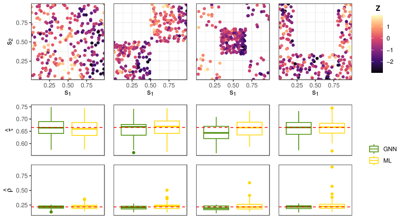
Figure 4: Several spatial data sets (top row) and empirical marginal sampling distributions (second and third rows) of two estimators for the Gaussian process model of Section 3.2 under a single parameter configuration (red dashed line). The estimators are the ML estimator (gold) and a GNN-based neural Bayes estimator (green). A single GNN was trained for all data sets.

Having established the efficacy of GNN-based point estimation, we next consider uncertainty quantification. Following our novel methodology described in Section 2.2.4, we construct a neural Bayes estimator that approximates the 0.025 and 0.975 marginal posterior quantiles, and use these to construct credible intervals with 95% nominal coverage. The training time is 52 minutes, while estimation from a single data set with $n=250$ locations takes 0.004 seconds. We assess these intervals by sampling 3000 parameter vectors from the prior distribution, simulating 10 data sets from the model for each parameter vector at $n=250$ locations, and computing the overall empirical coverage from these 30,000 data sets. The spatial locations vary with each data set, and are sampled from the Matérn cluster process used to train the estimator. The empirical coverages for $\tau$ and $\rho$ are 94.7% and 94.2%, respectively, which are close to the nominal value.

These results show that our GNN-based neural Bayes estimator is both performing as one would expect and that it can be applied to data sets with differing spatial configurations. For the Gaussian process model, inference with the likelihood function is feasible and neural Bayes estimators are usually not required unless we need to do estimation repeatedly, as we illustrate in Section 4. Neural Bayes estimators are particularly beneficial when the likelihood function is unavailable, as is the case for the model we consider next.

3.3 Schlather’s max-stable model

Max-stable processes are a central pillar of spatial extreme-value analysis (Davison_Huser_2015_Statistics_of_extremes; Davison_2019_spatial_extremes; Huser_2022_advances_in_spatial_extremes), being the only possible non-degenerate limits of properly renormalised pointwise block maxima of independent and identically distributed (i.i.d.) random fields. However, inference using the full likelihood function is computationally infeasible with even a moderate number of observed locations (Castruccio_2016_composite_likelihood_max-stable); they are, therefore, ideal candidates for likelihood-free inference. Here we consider Schlather’s max-stable model (Schlather_2002_max-stable_models), given by

$$Z_{ij}=\max_{k\in\mathbb{N}}\zeta_{ik}^{-1}\max\{0,Y_{ik}({\mathchoice{\hbox{\boldmath$\displaystyle{s}$}}{\hbox{\boldmath$\textstyle{s}$}}{\hbox{\boldmath$\scriptstyle{s}$}}{\hbox{\boldmath$\scriptscriptstyle{s}$}}}_{ij})\},\quad i=1,\dots,m,\;j=1,\dots,n_{i},$$ (13)

where, for replicates $i=1,\dots,m$, ${\mathchoice{\hbox{\boldmath$\displaystyle{Z}$}}{\hbox{\boldmath$\textstyle{Z}$}}{\hbox{\boldmath$\scriptstyle{Z}$}}{\hbox{\boldmath$\scriptscriptstyle{Z}$}}}_{i}\equiv(Z_{i1},\dots,Z_{in_{i}})^{\prime}$ are observed at locations $\{{\mathchoice{\hbox{\boldmath$\displaystyle{s}$}}{\hbox{\boldmath$\textstyle{s}$}}{\hbox{\boldmath$\scriptstyle{s}$}}{\hbox{\boldmath$\scriptscriptstyle{s}$}}}_{i1},\dots,{\mathchoice{\hbox{\boldmath$\displaystyle{s}$}}{\hbox{\boldmath$\textstyle{s}$}}{\hbox{\boldmath$\scriptstyle{s}$}}{\hbox{\boldmath$\scriptscriptstyle{s}$}}}_{in_{i}}\}\subset\mathcal{D}$, $\{\zeta_{ik}\mathrel{\mathop{\mathchar 58\relax}}k\in\mathbb{N}\}$ are i.i.d. Poisson point processes on $(0,\infty)$ with unit intensity, and $\{Y_{ik}(\cdot)\mathrel{\mathop{\mathchar 58\relax}}k\in\mathbb{N}\}$ are i.i.d. mean-zero Gaussian processes scaled so that $\mathbb{E}[{\max\{0,Y_{ik}(\cdot)\}}]=1$. Here, we model each $Y_{ik}(\cdot)$ using the Matérn covariance function (12), with $\sigma^{2}=1$. Hence, the unknown parameter vector to estimate is ${\mathchoice{\hbox{\boldmath$\displaystyle{\theta}$}}{\hbox{\boldmath$\textstyle{\theta}$}}{\hbox{\boldmath$\scriptstyle{\theta}$}}{\hbox{\boldmath$\scriptscriptstyle{\theta}$}}}\equiv(\rho,\nu)^{\prime}$.

We compare our GNN-based estimator to a likelihood-based estimator; however, for max-stable models, the likelihood function is computationally intractable, since the number of terms grows super-exponentially fast in the number of observed locations (see, e.g., Padoan_2010_composite_likelihood_max_stable_processes; Huser_2019_advances_in_spatial_extremes). A popular substitute is the pairwise likelihood (PL) function, a composite likelihood formed by considering only pairs of observed locations. Specifically, the pairwise log-likelihood function for the $i$th replicate is

$$\ell_{\rm{PL}}({\mathchoice{\hbox{\boldmath$\displaystyle{\theta}$}}{\hbox{\boldmath$\textstyle{\theta}$}}{\hbox{\boldmath$\scriptstyle{\theta}$}}{\hbox{\boldmath$\scriptscriptstyle{\theta}$}}};{\mathchoice{\hbox{\boldmath$\displaystyle{Z}$}}{\hbox{\boldmath$\textstyle{Z}$}}{\hbox{\boldmath$\scriptstyle{Z}$}}{\hbox{\boldmath$\scriptscriptstyle{Z}$}}}_{i})\equiv\sum_{j=1}^{n_{i}-1}\sum_{j^{\prime}=j+1}^{n_{i}}\omega^{(i)}_{jj^{\prime}}\log f(Z_{ij},Z_{ij^{\prime}}\mid{\mathchoice{\hbox{\boldmath$\displaystyle{\theta}$}}{\hbox{\boldmath$\textstyle{\theta}$}}{\hbox{\boldmath$\scriptstyle{\theta}$}}{\hbox{\boldmath$\scriptscriptstyle{\theta}$}}}),$$ (14)

where $f(\cdot,\cdot\mid{\mathchoice{\hbox{\boldmath$\displaystyle{\theta}$}}{\hbox{\boldmath$\textstyle{\theta}$}}{\hbox{\boldmath$\scriptstyle{\theta}$}}{\hbox{\boldmath$\scriptscriptstyle{\theta}$}}})$ denotes the bivariate probability density function for pairs in ${\mathchoice{\hbox{\boldmath$\displaystyle{Z}$}}{\hbox{\boldmath$\textstyle{Z}$}}{\hbox{\boldmath$\scriptstyle{Z}$}}{\hbox{\boldmath$\scriptscriptstyle{Z}$}}}_{i}$ (see Huser_2013_PhD_thesis, pg. 231–232) and $\omega^{(i)}_{jj^{\prime}}$ denotes a nonnegative weight. Hence, here we compare our GNN-based estimator to the maximum PL estimator. The computational and statistical efficiency of the PL estimator can often be improved by constructing (14) using only a subset of pairs that are within a fixed cut-off distance (Bevilacqua_2012; Sang_Genton_2014); here, we find that considering pairs within a distance of 0.2 units provides the best results and, therefore, we hereafter set $\omega^{(i)}_{jj^{\prime}}=\mathbb{I}(\|{\mathchoice{\hbox{\boldmath$\displaystyle{s}$}}{\hbox{\boldmath$\textstyle{s}$}}{\hbox{\boldmath$\scriptstyle{s}$}}{\hbox{\boldmath$\scriptscriptstyle{s}$}}}_{ij}-{\mathchoice{\hbox{\boldmath$\displaystyle{s}$}}{\hbox{\boldmath$\textstyle{s}$}}{\hbox{\boldmath$\scriptstyle{s}$}}{\hbox{\boldmath$\scriptscriptstyle{s}$}}}_{ij^{\prime}}\|\leq 0.2)$ in (14).

We use the priors $\rho\sim{\text{Unif}}(0.05,0.3)$ and $\nu\sim{\text{Unif}}(0.5,2.5)$, and we consider $m=20$ independent spatial fields for each parameter vector, with locations sampled during training according to the Matérn cluster process with $n=250$ locations on average, as in Section 3.1. The total training time for our GNN-based estimator is 2.6 hours. The PL estimator takes about 11.5 seconds to estimate the parameters from a single data set collected at $n=250$ locations, while the GNN-based estimator takes 0.002 seconds, a 5750-fold speedup post training. Figure 5 shows the empirical sampling distributions of both our GNN-based estimator and the PL estimator under a single parameter configuration but over four different spatial sample configurations. Both estimators are approximately unbiased, but the GNN-based estimator has substantially lower variance. Next, to quantify the overall performance of the estimators, we construct a test set of 1000 parameter vectors sampled from the prior distribution, and compute the empirical root-mean-squared error (RMSE) averaged over the spatial configurations shown in Figure 5. The RMSE of the GNN-based and PL estimator is 0.07 and 0.36, respectively; our GNN-based estimator thus provides a substantial reduction in RMSE over the PL estimator.

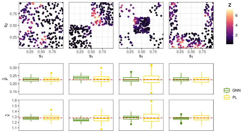
Figure S2: Several spatial data sets (top row) and corresponding empirical marginal sampling distributions (second and third rows) of two estimators for the Brown–Resnick max-stable model (Brown_Resnick_1977), with the same construction as given in Richards_2023_censoring. The estimators are the maximum-pairwise-likelihood (PL) estimator (gold) and a GNN-based neural Bayes estimator (green). A single GNN was trained for all data sets. The RMSE values of the GNN-based and PL estimators are 0.027 and 0.049, respectively. The PL estimator takes about 5.1 seconds to estimate the parameters from a single data set, while our GNN-based estimator takes 0.002 seconds post-training, a 2500-fold speedup.

Overall, the proposed GNN-based neural Bayes estimator is clearly superior to the composite-likelihood-based technique for Schlather’s max-stable model. We also considered the more popular Brown–Resnick max-stable process (Brown_Resnick_1977), which was previously used in the context of neural Bayes estimation by Lenzi_2021_NN_param_estimation and Richards_2023_censoring; our results, summarised in Figure S2 of the supplementary material, show that our GNN-based estimator again outperforms the conventional PL estimator (albeit to a lesser degree) and provides a substantial reduction in run time.

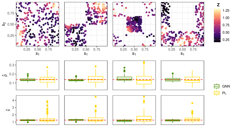
Figure 5: Several spatial data sets (top row) and corresponding empirical marginal sampling distributions (second and third rows) of two estimators for Schlather’s max-stable model of Section 3.3 under a single parameter configuration (red dashed line). The estimators are the maximum-pairwise-likelihood estimator (gold) and a GNN-based neural Bayes estimator (green). A single GNN was trained for all data sets.

4 Application to global sea-surface temperature

We now apply our methodology to the analysis of a massive global sea-surface temperature (SST) data set. Our application uses the data analysed by Zammit_2020 and Cressie_2021_review_spatial-basis-function_models, which consists of SST data obtained from the Visible Infrared Imaging Radiometer Suite (VIIRS) on board the Suomi National Polar-orbiting Partnership (Suomi NPP) weather satellite (Cao_2013_Suomi_NPP). The data set consists of 1,000,000 observed locations across the globe. As in Zammit_2020, we model the spatial residuals from a linear model with covariates given by an intercept, the latitude coordinate, and the square of the latitude coordinate. Figure 6 shows this detrended data set over the globe and in two equally-sized regions corresponding to the Brazil-Malvinas Confluence Zone and a region in the Indian Ocean. These regions provide clear evidence for spatial covariance non-stationarity in this data set.

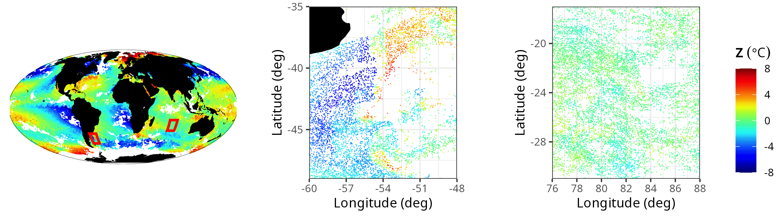
Figure 6: SST residuals over the globe (left), in the Brazil-Malvinas Confluence Zone (centre), and in the Indian Ocean (right). These regions, which are demarcated by red rectangles in the left panel, illustrate the spatial non-stationarity present in this data set.

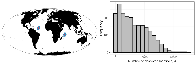
Figure S3: (Left) Two cell clusters used in the application study of Section 4; the parameter estimates for a given cell (red) are obtained using both the data within that cell and the data within its neighbouring cells (blue). (Right) Histogram of the number of observed locations, $n$, for all cell clusters used in the application study of Section 4.

To account for spatial covariance non-stationarity, we use a local modelling approach by partitioning the spatial domain and fitting a separate model within each region. Our partition is the ISEA Aperture 3 Hexagon (ISEA3H) discrete global grid (DGG) at resolution 5, which contains 2,432 equally-sized hexagonal cells. We model the dependence structure within each hexagon using the Gaussian process model of Section 3.2, with unknown range parameter, $\rho$, process standard deviation, $\sigma$, and measurement-error standard deviation, $\tau$. Therefore, within each cell, we estimate three unknown parameters, ${\mathchoice{\hbox{\boldmath$\displaystyle{\theta}$}}{\hbox{\boldmath$\textstyle{\theta}$}}{\hbox{\boldmath$\scriptstyle{\theta}$}}{\hbox{\boldmath$\scriptscriptstyle{\theta}$}}}\equiv(\rho,\sigma,\tau)^{\prime}$. We adopt a moving-window approach (Haas_1990_moving_window; Haas_1990_moving_window_lognormal; Castro-Camilo_2020_local_estimation) to parameter estimation, whereby the parameter estimates for a given cell are obtained using both the data within that cell and the data within its neighbouring cells. We refer to a cell and its neighbours as a cell cluster; the left panel of Figure S3 of the supplementary material shows an example of two cell clusters. This moving-window approach makes large-scale trends more apparent, facilitates the exploration of covariance non-stationarity, and it makes estimation both more efficient (through the use of more data), as well as possible in unobserved cells, provided that neighbouring cells contain data. In total, there are 2,161 cell clusters that contain data to make inference with, and these clusters contain a median number of $2,769$ observed locations, and a maximum of $12,591$ observed locations; the right panel of Figure S3 shows a histogram of the number of observed locations for all cell clusters.

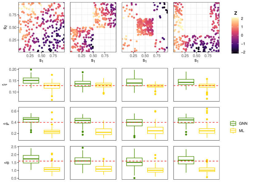
Figure S4: Several spatial data sets (top row), each with $n=250$ spatial locations, and empirical marginal sampling distributions (second, third, and fourth rows) of two estimators for the Gaussian process model of Section 4 under a single parameter configuration (red dashed line). The estimators are the ML estimator (gold) and a GNN-based neural Bayes estimator (green). A single GNN was trained for all data sets. We assessed our neural interval estimator in the same manner described in Section 3.2; the empirical coverages for $\tau$, $\rho$, and $\sigma$ were 95.6%, 94.9%, and 94.6%, respectively, which are close to the nominal value of 95%. Here the neural Bayes estimator outperforms the ML estimator, likely because the parameters are weakly identifiable in this model, which makes the likelihood function relatively flat in the region of its mode.

For point estimation, we use a single GNN-based neural Bayes estimator trained under the mean-absolute-error loss. For uncertainty quantification, we obtain credible intervals by approximating the 0.025 and 0.975 marginal posterior quantiles jointly using a single GNN-based neural Bayes estimator, as described in Section 2.2.4. We use the same architectures described in Section 3.1. We validate our trained estimators using the approach taken in Section 3; see Figure S4 of the supplementary material. Since the amount of data available varies between cell clusters, we train our estimator using simulated spatial data sets with variable sample sizes; each set of spatial configurations, $\textstyle{S}$, used to construct the training data are sampled from a Matérn cluster process (see Figure 2) on the unit square, with the expected number of sampled points varying between $n=30$ and $n=2000$. To estimate the parameters in cell clusters with a higher number of observed locations, we make use of the estimator’s ability to extrapolate to larger values of $n$ than those used during training (a property illustrated and discussed in Section S1 of the supplementary material). Note that we could train our estimator with a prior distribution on $n$ based on the distribution of sample sizes in our data set, shown in Figure S3; however, we choose not to do so since we prefer to illustrate the use of a single, broadly-applicable GNN-based neural Bayes estimator, rather than one tailored specifically to this data set. Since we train our estimator using spatial locations sampled within the unit square, our estimator is calibrated for distances within $[0,\sqrt{2}]$. Therefore, as a pre-processing step, we scale the distances within each cell cluster to be within this range, where the distance measure is the chordal distance, and the estimated range parameter is then similarly scaled back for interpretation after it is estimated. Note that use of the chordal distance is justified by the small size of the cells: it is reasonable to model the Earth’s surface as approximately flat within the cell clusters. We assume our parameters are independent a priori with marginal priors $\rho\sim{\text{Unif}}(0.05,0.60)$, $\sigma\sim{\text{Unif}}(0.1,3.0)$, and $\tau\sim{\text{Unif}}(0.1,1.0)$. The total training time for our point and credible-interval estimators is about 4 hours.

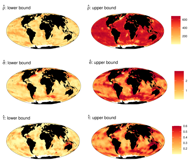
Figure S5: Spatially varying estimates of the marginal 0.025 quantile (left column) and marginal 0.975 quantile (right column) used as lower and upper bounds, respectively, for each parameter of the Gaussian process model used in Section 4. The first, second, and third rows correspond to the range parameter, $\rho$, process standard deviation, $\sigma$, and measurement-error standard deviation, $\tau$, respectively. The globe is partitioned using the ISEA Aperture 3 Hexagon (ISEA3H) discrete global grid (DGG) at resolution 5.

Figure 7 shows spatially varying point estimates and 95% credible-interval widths for each parameter. Figure S5 of the supplementary material shows estimates of the 0.025 and 0.975 quantiles. Our neural Bayes estimators provide point estimates and credible intervals over 2,161 cell clusters in just over three minutes. The point estimates given in Figure 7 conform with what one may expect when modelling global SST: energetic regions, for example, near the South-East coast of South America, tend to exhibit large estimates of the process standard deviation, $\sigma$, and small estimates of the length scale $\rho$; by contrast, more stable regions, such as those towards the centre of large ocean basins, tend to exhibit small estimates of $\sigma$ and larger estimates of $\rho$.

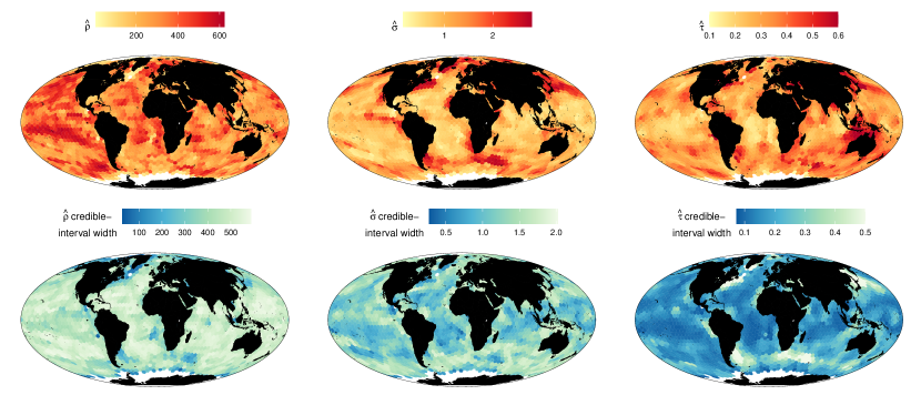
Figure 7: Spatially varying point estimates (top row) and corresponding 95% credible-interval widths (bottom row) for each parameter of the Gaussian process model used to analyse global SST in Section 4. The first, second, and third columns correspond to the range parameter, $\rho$, process standard deviation, $\sigma$, and measurement-error standard deviation, $\tau$. The globe is partitioned using the ISEA Aperture 3 Hexagon (ISEA3H) discrete global grid (DGG) at resolution 5.

5 Conclusion

In this paper, we develop a new approach for neural Bayes estimation from irregular spatial data that uses GNNs. Our approach has two main strengths. First, GNN-based neural Bayes estimators are specifically designed to capture spatial dependence, and are thus parsimonious approximators of Bayes estimators in spatial settings. Second, GNN-based estimators can be applied to data collected over any set of spatial locations, which allows the computationally-intensive training step to be amortised for a given spatial model. That is, a single GNN-based estimator can be re-used for new spatial data sets irrespective of the new observation locations. Importantly, we have also shown how to combine the GNN architecture with the DeepSets framework to construct a neural Bayes estimator applicable with any number of independent replicates, thus opening the door to amortised estimation in a wide range of application settings for arbitrary spatial models. We have also provided implementation guidelines, in particular for those pertaining to neural-network architecture design and the construction of synthetic spatial data sets for training the estimators, and we have proposed a novel approach to uncertainty quantification via a suitably designed neural Bayes estimator that approximates a set of marginal posterior quantiles (approximated jointly to avoid quantile crossing). Finally, we provide user-friendly access to our methodology by incorporating it within the package NeuralEstimators (Sainsbury-Dale_2022_neural_Bayes_estimators), which is available in the Julia and R programming languages.

We have considered inference from irregular spatial data; the extension to irregular spatio-temporal data using spatio-temporal GNNs (Wu_2021_GNN_review, Sec. VII) is the subject of future work. GNNs also extend naturally to multivariate spatial processes (Gneiting_2010_multivariate_Matern; Apanasovich_2012_multivariate_Matern; Genton_2015_multivariate_geostatistics; Genton_2015_multivariate_maxstable_processes), although the often complicated parameter constraints in these settings require careful consideration. We have focused on point estimation; GNNs, however, would also be useful for approximating the full posterior distribution, for instance by incorporating them as a module in a normalising flow (Radev_2022_BayesFlow) or a generative adversarial network (GAN; Pacchiardi_2022_GANs_scoring_rules), or by using them to automatically learn relevant summary statistics in approximate Bayesian computation (ABC; see, e.g., Jiang_2017; Chen_2021_NN-approximate_sufficient_statistics_for_implicit_models). GNNs may also prove useful in recent neural approaches to approximating the likelihood function (Walchessen_2023_neural_likelihood_surfaces). It is also straightforward to combine GNNs with the censoring framework of Richards_2023_censoring, in order to perform neural Bayes estimation from censored data collected over arbitrary spatial locations. Finally, GNNs may prove useful in non-spatial applications; for example, exponential random graph models (ERGMs; Robins_2007_ERGMs; Lusher_2013_ERGMs) used in network analysis have a normalising constant that prevents straightforward evaluation of the likelihood function, and would therefore likely benefit from the proposed likelihood-free inference framework.

Appendix A Bayes estimators under additive loss functions

Theorem 1.

Let $\mathcal{P}\equiv\{P_{{\mathchoice{\hbox{\boldmath$\displaystyle{\theta}$}}{\hbox{\boldmath$\textstyle{\theta}$}}{\hbox{\boldmath$\scriptstyle{\theta}$}}{\hbox{\boldmath$\scriptscriptstyle{\theta}$}}}}\mathrel{\mathop{\mathchar 58\relax}}{\mathchoice{\hbox{\boldmath$\displaystyle{\theta}$}}{\hbox{\boldmath$\textstyle{\theta}$}}{\hbox{\boldmath$\scriptstyle{\theta}$}}{\hbox{\boldmath$\scriptscriptstyle{\theta}$}}}\in\Theta\}$ denote a class of distributions parameterised by the $p$-dimensional vector $\textstyle{\theta}$, and suppose that we have observed data ${\mathchoice{\hbox{\boldmath$\displaystyle{z}$}}{\hbox{\boldmath$\textstyle{z}$}}{\hbox{\boldmath$\scriptstyle{z}$}}{\hbox{\boldmath$\scriptscriptstyle{z}$}}}\sim P_{{\mathchoice{\hbox{\boldmath$\displaystyle{\theta}$}}{\hbox{\boldmath$\textstyle{\theta}$}}{\hbox{\boldmath$\scriptstyle{\theta}$}}{\hbox{\boldmath$\scriptscriptstyle{\theta}$}}}}$ that is an element of the sample space $\mathcal{S}$. Let $L(\cdot,\cdot)$ denote a loss function of the form

$$L({\mathchoice{\hbox{\boldmath$\displaystyle{\theta}$}}{\hbox{\boldmath$\textstyle{\theta}$}}{\hbox{\boldmath$\scriptstyle{\theta}$}}{\hbox{\boldmath$\scriptscriptstyle{\theta}$}}},\hat{{\mathchoice{\hbox{\boldmath$\displaystyle{\theta}$}}{\hbox{\boldmath$\textstyle{\theta}$}}{\hbox{\boldmath$\scriptstyle{\theta}$}}{\hbox{\boldmath$\scriptscriptstyle{\theta}$}}}}({\mathchoice{\hbox{\boldmath$\displaystyle{z}$}}{\hbox{\boldmath$\textstyle{z}$}}{\hbox{\boldmath$\scriptstyle{z}$}}{\hbox{\boldmath$\scriptscriptstyle{z}$}}}))\equiv\sum_{k=1}^{p}\tilde{L}_{k}(\theta_{k},\hat{\theta}_{k}({\mathchoice{\hbox{\boldmath$\displaystyle{z}$}}{\hbox{\boldmath$\textstyle{z}$}}{\hbox{\boldmath$\scriptstyle{z}$}}{\hbox{\boldmath$\scriptscriptstyle{z}$}}})),$$ (15)

where $\hat{{\mathchoice{\hbox{\boldmath$\displaystyle{\theta}$}}{\hbox{\boldmath$\textstyle{\theta}$}}{\hbox{\boldmath$\scriptstyle{\theta}$}}{\hbox{\boldmath$\scriptscriptstyle{\theta}$}}}}(\cdot)\equiv(\hat{\theta}_{1}(\cdot),\dots,\hat{\theta}_{p}(\cdot))^{\prime}$ is an estimator of $\textstyle{\theta}$ and, for $k=1,\dots,p$, $\tilde{L}_{k}(\cdot,\cdot)$ is a univariate loss function. Then a Bayes estimator under $L(\cdot,\cdot)$ is given by $(\hat{\theta}_{1}^{\star}(\cdot),\dots,\hat{\theta}_{p}^{\star}(\cdot))^{\prime}$ where, for $k=1,\dots,p$, $\hat{\theta}_{k}^{\star}(\cdot)$ is the marginal Bayes estimator for $\theta_{k}$ under the loss $\tilde{L}_{k}(\cdot,\cdot)$.

• Here, for ease of exposition, we give the proof for the case where the posterior distribution ${\mathchoice{\hbox{\boldmath$\displaystyle{\theta}$}}{\hbox{\boldmath$\textstyle{\theta}$}}{\hbox{\boldmath$\scriptstyle{\theta}$}}{\hbox{\boldmath$\scriptscriptstyle{\theta}$}}}\mid{\mathchoice{\hbox{\boldmath$\displaystyle{z}$}}{\hbox{\boldmath$\textstyle{z}$}}{\hbox{\boldmath$\scriptstyle{z}$}}{\hbox{\boldmath$\scriptscriptstyle{z}$}}}$ admits a density function with respect to Lebesgue measure. For generic random quantities $A$ and $B$, we use $[A\mid B]$ to denote the conditional probability density function of $A$ given $B$. We use ${\mathchoice{\hbox{\boldmath$\displaystyle{\theta}$}}{\hbox{\boldmath$\textstyle{\theta}$}}{\hbox{\boldmath$\scriptstyle{\theta}$}}{\hbox{\boldmath$\scriptscriptstyle{\theta}$}}}_{\setminus k}$ to denote the vector $\textstyle{\theta}$ with its $k$th element removed; similarly, $\Theta_{k}$ and $\Theta_{\setminus k}$ denote the parameter spaces of $\theta_{k}$ and ${\mathchoice{\hbox{\boldmath$\displaystyle{\theta}$}}{\hbox{\boldmath$\textstyle{\theta}$}}{\hbox{\boldmath$\scriptstyle{\theta}$}}{\hbox{\boldmath$\scriptscriptstyle{\theta}$}}}_{\setminus k}$, respectively. Now, provided that the Bayes risk is finite, a Bayes estimator is obtained by minimising the conditional risk (i.e., the expected posterior loss),

  $$\int_{\Theta}L({\mathchoice{\hbox{\boldmath$\displaystyle{\theta}$}}{\hbox{\boldmath$\textstyle{\theta}$}}{\hbox{\boldmath$\scriptstyle{\theta}$}}{\hbox{\boldmath$\scriptscriptstyle{\theta}$}}},\hat{{\mathchoice{\hbox{\boldmath$\displaystyle{\theta}$}}{\hbox{\boldmath$\textstyle{\theta}$}}{\hbox{\boldmath$\scriptstyle{\theta}$}}{\hbox{\boldmath$\scriptscriptstyle{\theta}$}}}}({\mathchoice{\hbox{\boldmath$\displaystyle{z}$}}{\hbox{\boldmath$\textstyle{z}$}}{\hbox{\boldmath$\scriptstyle{z}$}}{\hbox{\boldmath$\scriptscriptstyle{z}$}}}))[{\mathchoice{\hbox{\boldmath$\displaystyle{\theta}$}}{\hbox{\boldmath$\textstyle{\theta}$}}{\hbox{\boldmath$\scriptstyle{\theta}$}}{\hbox{\boldmath$\scriptscriptstyle{\theta}$}}}\mid{\mathchoice{\hbox{\boldmath$\displaystyle{z}$}}{\hbox{\boldmath$\textstyle{z}$}}{\hbox{\boldmath$\scriptstyle{z}$}}{\hbox{\boldmath$\scriptscriptstyle{z}$}}}]\textrm{d}{\mathchoice{\hbox{\boldmath$\displaystyle{\theta}$}}{\hbox{\boldmath$\textstyle{\theta}$}}{\hbox{\boldmath$\scriptstyle{\theta}$}}{\hbox{\boldmath$\scriptscriptstyle{\theta}$}}},$$ (16)

  for all ${\mathchoice{\hbox{\boldmath$\displaystyle{z}$}}{\hbox{\boldmath$\textstyle{z}$}}{\hbox{\boldmath$\scriptstyle{z}$}}{\hbox{\boldmath$\scriptscriptstyle{z}$}}}\in\mathcal{S}$ (e.g., Lehmann_Casella_1998_Point_Estimation, Lehmann_Casella_1998_Point_Estimation, Ch. 4, Thm. 1.1; Robert_2007_The_Bayesian_Choice, Robert_2007_The_Bayesian_Choice, Thm. 2.3.2). Under the loss function (15), the conditional risk (16) is

  $$\int_{\Theta}L({\mathchoice{\hbox{\boldmath$\displaystyle{\theta}$}}{\hbox{\boldmath$\textstyle{\theta}$}}{\hbox{\boldmath$\scriptstyle{\theta}$}}{\hbox{\boldmath$\scriptscriptstyle{\theta}$}}},\hat{{\mathchoice{\hbox{\boldmath$\displaystyle{\theta}$}}{\hbox{\boldmath$\textstyle{\theta}$}}{\hbox{\boldmath$\scriptstyle{\theta}$}}{\hbox{\boldmath$\scriptscriptstyle{\theta}$}}}}({\mathchoice{\hbox{\boldmath$\displaystyle{z}$}}{\hbox{\boldmath$\textstyle{z}$}}{\hbox{\boldmath$\scriptstyle{z}$}}{\hbox{\boldmath$\scriptscriptstyle{z}$}}}))[{\mathchoice{\hbox{\boldmath$\displaystyle{\theta}$}}{\hbox{\boldmath$\textstyle{\theta}$}}{\hbox{\boldmath$\scriptstyle{\theta}$}}{\hbox{\boldmath$\scriptscriptstyle{\theta}$}}}\mid{\mathchoice{\hbox{\boldmath$\displaystyle{z}$}}{\hbox{\boldmath$\textstyle{z}$}}{\hbox{\boldmath$\scriptstyle{z}$}}{\hbox{\boldmath$\scriptscriptstyle{z}$}}}]\textrm{d}{\mathchoice{\hbox{\boldmath$\displaystyle{\theta}$}}{\hbox{\boldmath$\textstyle{\theta}$}}{\hbox{\boldmath$\scriptstyle{\theta}$}}{\hbox{\boldmath$\scriptscriptstyle{\theta}$}}} =\int_{\Theta}\sum_{k=1}^{p}\tilde{L}_{k}(\theta_{k},\hat{\theta}_{k}({\mathchoice{\hbox{\boldmath$\displaystyle{z}$}}{\hbox{\boldmath$\textstyle{z}$}}{\hbox{\boldmath$\scriptstyle{z}$}}{\hbox{\boldmath$\scriptscriptstyle{z}$}}}))[{\mathchoice{\hbox{\boldmath$\displaystyle{\theta}$}}{\hbox{\boldmath$\textstyle{\theta}$}}{\hbox{\boldmath$\scriptstyle{\theta}$}}{\hbox{\boldmath$\scriptscriptstyle{\theta}$}}}\mid{\mathchoice{\hbox{\boldmath$\displaystyle{z}$}}{\hbox{\boldmath$\textstyle{z}$}}{\hbox{\boldmath$\scriptstyle{z}$}}{\hbox{\boldmath$\scriptscriptstyle{z}$}}}]\textrm{d}{\mathchoice{\hbox{\boldmath$\displaystyle{\theta}$}}{\hbox{\boldmath$\textstyle{\theta}$}}{\hbox{\boldmath$\scriptstyle{\theta}$}}{\hbox{\boldmath$\scriptscriptstyle{\theta}$}}}$$

  $$=\sum_{k=1}^{p}\int_{\Theta}\tilde{L}_{k}(\theta_{k},\hat{\theta}_{k}({\mathchoice{\hbox{\boldmath$\displaystyle{z}$}}{\hbox{\boldmath$\textstyle{z}$}}{\hbox{\boldmath$\scriptstyle{z}$}}{\hbox{\boldmath$\scriptscriptstyle{z}$}}}))[\theta_{k}\mid{\mathchoice{\hbox{\boldmath$\displaystyle{z}$}}{\hbox{\boldmath$\textstyle{z}$}}{\hbox{\boldmath$\scriptstyle{z}$}}{\hbox{\boldmath$\scriptscriptstyle{z}$}}}][{\mathchoice{\hbox{\boldmath$\displaystyle{\theta}$}}{\hbox{\boldmath$\textstyle{\theta}$}}{\hbox{\boldmath$\scriptstyle{\theta}$}}{\hbox{\boldmath$\scriptscriptstyle{\theta}$}}}_{\setminus k}\mid\theta_{k},{\mathchoice{\hbox{\boldmath$\displaystyle{z}$}}{\hbox{\boldmath$\textstyle{z}$}}{\hbox{\boldmath$\scriptstyle{z}$}}{\hbox{\boldmath$\scriptscriptstyle{z}$}}}]\textrm{d}{\mathchoice{\hbox{\boldmath$\displaystyle{\theta}$}}{\hbox{\boldmath$\textstyle{\theta}$}}{\hbox{\boldmath$\scriptstyle{\theta}$}}{\hbox{\boldmath$\scriptscriptstyle{\theta}$}}}$$

  $$=\sum_{k=1}^{p}\int_{\Theta_{k}}\tilde{L}_{k}(\theta_{k},\hat{\theta}_{k}({\mathchoice{\hbox{\boldmath$\displaystyle{z}$}}{\hbox{\boldmath$\textstyle{z}$}}{\hbox{\boldmath$\scriptstyle{z}$}}{\hbox{\boldmath$\scriptscriptstyle{z}$}}}))[\theta_{k}\mid{\mathchoice{\hbox{\boldmath$\displaystyle{z}$}}{\hbox{\boldmath$\textstyle{z}$}}{\hbox{\boldmath$\scriptstyle{z}$}}{\hbox{\boldmath$\scriptscriptstyle{z}$}}}]\left(\int_{\Theta_{\setminus k}}[{\mathchoice{\hbox{\boldmath$\displaystyle{\theta}$}}{\hbox{\boldmath$\textstyle{\theta}$}}{\hbox{\boldmath$\scriptstyle{\theta}$}}{\hbox{\boldmath$\scriptscriptstyle{\theta}$}}}_{\setminus k}\mid\theta_{k},{\mathchoice{\hbox{\boldmath$\displaystyle{z}$}}{\hbox{\boldmath$\textstyle{z}$}}{\hbox{\boldmath$\scriptstyle{z}$}}{\hbox{\boldmath$\scriptscriptstyle{z}$}}}]\textrm{d}{\mathchoice{\hbox{\boldmath$\displaystyle{\theta}$}}{\hbox{\boldmath$\textstyle{\theta}$}}{\hbox{\boldmath$\scriptstyle{\theta}$}}{\hbox{\boldmath$\scriptscriptstyle{\theta}$}}}_{\setminus k}\right)\textrm{d}\theta_{k}$$

  $$=\sum_{k=1}^{p}\int_{\Theta_{k}}\tilde{L}_{k}(\theta_{k},\hat{\theta}_{k}({\mathchoice{\hbox{\boldmath$\displaystyle{z}$}}{\hbox{\boldmath$\textstyle{z}$}}{\hbox{\boldmath$\scriptstyle{z}$}}{\hbox{\boldmath$\scriptscriptstyle{z}$}}}))[\theta_{k}\mid{\mathchoice{\hbox{\boldmath$\displaystyle{z}$}}{\hbox{\boldmath$\textstyle{z}$}}{\hbox{\boldmath$\scriptstyle{z}$}}{\hbox{\boldmath$\scriptscriptstyle{z}$}}}]\textrm{d}\theta_{k}.$$

  which is minimised by minimising $\int_{\Theta_{k}}\tilde{L}_{k}(\theta_{k},\hat{\theta}_{k}({\mathchoice{\hbox{\boldmath$\displaystyle{z}$}}{\hbox{\boldmath$\textstyle{z}$}}{\hbox{\boldmath$\scriptstyle{z}$}}{\hbox{\boldmath$\scriptscriptstyle{z}$}}}))[\theta_{k}\mid{\mathchoice{\hbox{\boldmath$\displaystyle{z}$}}{\hbox{\boldmath$\textstyle{z}$}}{\hbox{\boldmath$\scriptstyle{z}$}}{\hbox{\boldmath$\scriptscriptstyle{z}$}}}]\textrm{d}\theta_{k}$ for each $k=1,\dots,p$. Therefore, for $k=1,\dots,p$, $\hat{\theta}_{k}^{\star}(\cdot)$ is a marginal Bayes estimator with respect to the loss $\tilde{L}_{k}(\cdot,\cdot)$. ∎

The estimator $\hat{\theta}_{k}^{\star}(\cdot)$, $k=1,\dots,p$, is a functional of the marginal posterior distribution of $\theta_{k}$, where the functional is the usual Bayes estimator with respect to $\tilde{L}_{k}(\cdot,\cdot)$. For example, if $\tilde{L}_{k}(\cdot,\cdot)$ is the absolute-error loss, then $\hat{\theta}_{k}^{\star}(\cdot)$ is the marginal posterior median of $\theta_{k}$.

In Section S1, we illustrate how our GNN-based neural Bayes estimators depend on the number of spatial locations. In Section S2, we provide additional figures and tables for the analysis given in the main text.

Appendix S1 Variable numbers of spatial locations

As discussed in the main text, a GNN-based neural Bayes estimator can be applied to data collected over any set of spatial locations, and with any number of locations, $n$. However, Bayes estimators are generally a function of $n$, and this must be taken into account during training if we wish the estimator to generalise over a wide range of possible sample sizes. Here, we illustrate how our GNN-based neural Bayes estimators depend on the sample size $n$ used during the training phase. We train several GNN-based neural Bayes estimators (with the same set-up described in Section 3.1 of the main text) for the Gaussian process model described in Section 3.2 of the main text: we train the estimators $\hat{{\mathchoice{\hbox{\boldmath$\displaystyle{\theta}$}}{\hbox{\boldmath$\textstyle{\theta}$}}{\hbox{\boldmath$\scriptstyle{\theta}$}}{\hbox{\boldmath$\scriptscriptstyle{\theta}$}}}}(\cdot;{\mathchoice{\hbox{\boldmath$\displaystyle{\gamma}$}}{\hbox{\boldmath$\textstyle{\gamma}$}}{\hbox{\boldmath$\scriptstyle{\gamma}$}}{\hbox{\boldmath$\scriptscriptstyle{\gamma}$}}}^{*}_{\scaleto{30}{5pt}})$ and $\hat{{\mathchoice{\hbox{\boldmath$\displaystyle{\theta}$}}{\hbox{\boldmath$\textstyle{\theta}$}}{\hbox{\boldmath$\scriptstyle{\theta}$}}{\hbox{\boldmath$\scriptscriptstyle{\theta}$}}}}(\cdot;{\mathchoice{\hbox{\boldmath$\displaystyle{\gamma}$}}{\hbox{\boldmath$\textstyle{\gamma}$}}{\hbox{\boldmath$\scriptstyle{\gamma}$}}{\hbox{\boldmath$\scriptscriptstyle{\gamma}$}}}^{*}_{\scaleto{1000}{5pt}})$ with spatial data sets containing exactly 30 or 1000 sampled locations, respectively, and we train the estimator $\hat{{\mathchoice{\hbox{\boldmath$\displaystyle{\theta}$}}{\hbox{\boldmath$\textstyle{\theta}$}}{\hbox{\boldmath$\scriptstyle{\theta}$}}{\hbox{\boldmath$\scriptscriptstyle{\theta}$}}}}(\cdot;{\mathchoice{\hbox{\boldmath$\displaystyle{\gamma}$}}{\hbox{\boldmath$\textstyle{\gamma}$}}{\hbox{\boldmath$\scriptstyle{\gamma}$}}{\hbox{\boldmath$\scriptscriptstyle{\gamma}$}}}^{*}_{\scaleto{30\mathrel{\mathop{\mathchar 58\relax}}1000}{5pt}})$ with $n$ treated as a discrete uniform random variable with support between 30 and 1000 inclusive. Irrespective of $n$, all spatial configurations are sampled uniformly over the unit square.

Figure S1, left panel, shows the empirical RMSE for each estimator evaluated over a test set of 1,000 parameter vectors, against the number of spatial locations, $n$. The estimators trained with fixed $n$ perform reasonably well when $n$ is close to the value used during training, but poorly for other sample sizes. On the other hand, the estimator $\hat{{\mathchoice{\hbox{\boldmath$\displaystyle{\theta}$}}{\hbox{\boldmath$\textstyle{\theta}$}}{\hbox{\boldmath$\scriptstyle{\theta}$}}{\hbox{\boldmath$\scriptscriptstyle{\theta}$}}}}(\cdot;{\mathchoice{\hbox{\boldmath$\displaystyle{\gamma}$}}{\hbox{\boldmath$\textstyle{\gamma}$}}{\hbox{\boldmath$\scriptstyle{\gamma}$}}{\hbox{\boldmath$\scriptscriptstyle{\gamma}$}}}^{*}_{\scaleto{30\mathrel{\mathop{\mathchar 58\relax}}1000}{5pt}})$ performs well for all $n\in\{30,\dots,1000\}$. All of the GNN-based neural Bayes estimators have some capacity to extrapolate to larger values of $n$ than those used during training, with the RMSE continuing to reduce slightly beyond the values of $n$ used during training. For small $n$, the maximum likelihood (ML) estimator is outperformed by the neural Bayes estimators trained for small samples, likely because the ML estimator is only asymptotically efficient with no finite sample guarantees. For large $n$, the ML estimator slightly outperforms the neural Bayes estimators trained with large values of $n$, likely because of some non-neglible error in our neural approximation of the Bayes estimator.

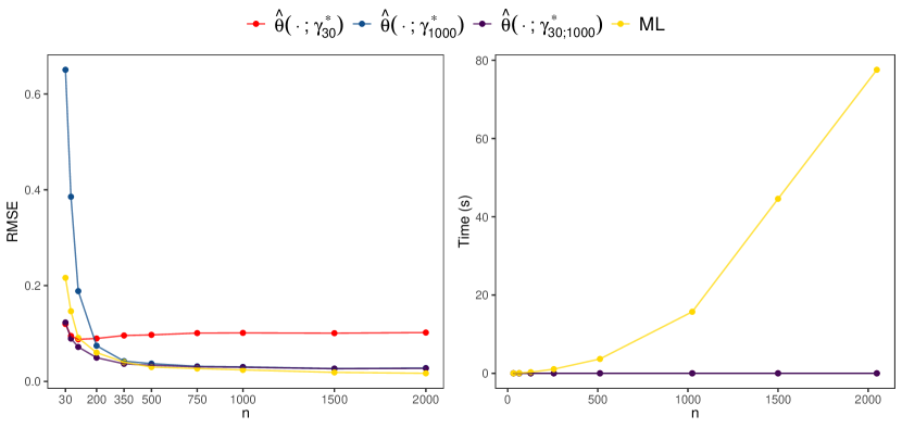
Figure S1: (Left) The RMSE against the number of spatial locations, $n$, for several estimators of the Gaussian process model of Section 3.2 of the main text. The estimators are the ML estimator (yellow) and several GNN-based neural Bayes estimators trained with either $n$ fixed to $30$ (red) or $1000$ (blue), or with $n$ sampled uniformly between $30$ and $1000$ (purple). (Right) The run time to estimate a single parameter vector against the sample size, $n$.

Figure S1, right panel, shows the run time (in seconds) to estimate a single parameter vector, against the number of spatial locations, $n$. The trained neural Bayes estimators have excellent computational properties with respect to $n$, since the computations involved in GNNs can be done in parallel and, therefore, are amenable to graphics processing units (GPUs) containing thousands of cores. By contrast, the computational bottleneck for ML estimation, the factorisation of an $n\times n$ covariance matrix, cannot be done in parallel without approximations, and is well known to have a computational complexity of $\mathcal{O}(n^{3})$. Note that ML estimation was performed using central processing units (CPUs).

Appendix S2 Additional figures and tables

Table S1: Summary of the neural-network architecture used in Sections 3 and 4. We follow the convention of reporting the dimension of the input and output of each layer, here using the notation $\{[q]\mathrel{\mathop{\mathchar 58\relax}}n\}$ to denote a set of $n$ vectors of length $q$ and, similarly, using $\{[q]\mathrel{\mathop{\mathchar 58\relax}}n\mathrel{\mathop{\mathchar 58\relax}}m\}$ to denote $m$ sets of $n$ vectors of length $q$. (Note that $n$, which in our work corresponds to the number of spatial locations, is allowed to vary between sets, but we do not make this explicit for notational convenience.) For all layers except the final layer we use a rectified linear unit (ReLU) activation function. For the final layer, we use an exponential activation function for positive parameters, and an identity activation function otherwise.

Module	Layer type	Input dimension	Output dimension	Parameters
propagation	graph conv	$\{[1]\mathrel{\mathop{\mathchar 58\relax}}n\mathrel{\mathop{\mathchar 58\relax}}m\}$	$\{[128]\mathrel{\mathop{\mathchar 58\relax}}n\mathrel{\mathop{\mathchar 58\relax}}m\}$	385
propagation	graph conv	$\{[128]\mathrel{\mathop{\mathchar 58\relax}}n\mathrel{\mathop{\mathchar 58\relax}}m\}$	$\{[128]\mathrel{\mathop{\mathchar 58\relax}}n\mathrel{\mathop{\mathchar 58\relax}}m\}$	32,897
propagation	graph conv	$\{[128]\mathrel{\mathop{\mathchar 58\relax}}n\mathrel{\mathop{\mathchar 58\relax}}m\}$	$\{[128]\mathrel{\mathop{\mathchar 58\relax}}n\mathrel{\mathop{\mathchar 58\relax}}m\}$	32,897
propagation	graph conv	$\{[128]\mathrel{\mathop{\mathchar 58\relax}}n\mathrel{\mathop{\mathchar 58\relax}}m\}$	$\{[128]\mathrel{\mathop{\mathchar 58\relax}}n\mathrel{\mathop{\mathchar 58\relax}}m\}$	32,897
readout	average	$\{[128]\mathrel{\mathop{\mathchar 58\relax}}n\mathrel{\mathop{\mathchar 58\relax}}m\}$	$\{[128]\mathrel{\mathop{\mathchar 58\relax}}m\}$	0
DeepSets agg.	average	$\{[128]\mathrel{\mathop{\mathchar 58\relax}}m\}$	$[128]$	0
mapping	dense	[128]	[128]	16,512
mapping	dense	[128]	[128]	16,512
mapping	dense	[128]	[$p$]	$129p$
Total trainable parameters:				132,100 + 129$p$

References

- Apanasovich et al., (2012) Apanasovich, T. V., Genton, M. G., and Sun, Y. (2012). A valid Matérn class of cross-covariance functions for multivariate random fields with any number of components. Journal of the American Statistical Association, 497:180–193.
- Baddeley et al., (2015) Baddeley, A., Rubak, E., and Turner, R. (2015). Spatial Point Patterns: Methodology and Applications with R. Chapman & Hall/CRC, Boca Raton, FL.
- Banesh et al., (2021) Banesh, D., Panda, N., Biswas, A., Roekel, L. V., Oyen, D., Urban, N., Grosskopf, M., Wolfe, J., and Lawrence, E. (2021). Fast Gaussian process estimation for large-scale in situ inference using convolutional neural networks. In IEEE International Conference on Big Data, pages 3731–3739.
- Bevilacqua et al., (2012) Bevilacqua, M., Gaetan, C., Mateu, J., and Porcu, E. (2012). Estimating space and space-time covariance functions for large data sets: A weighted composite likelihood approach. Journal of the American Statistical Association, 107:268–280.
- Brown and Resnick, (1977) Brown, B. M. and Resnick, S. I. (1977). Extreme values of independent stochastic processes. Journal of Applied Probability, 14:732–739.
- Cao et al., (2013) Cao, C., Xiong, J., Blonski, S., Liu, Q., Uprety, S., Shao, X., Bai, Y., and Weng, F. (2013). Suomi NPP VIIRS sensor data record verification, validation, and long-term performance monitoring. Journal of Geophysical Research: Atmospheres, 118:11–664.
- Castro-Camilo and Huser, (2020) Castro-Camilo, D. and Huser, R. (2020). Local likelihood estimation of complex tail dependence structures, applied to U.S. precipitation extremes. Journal of the American Statistical Association, 115:1037–1054.
- Castruccio et al., (2016) Castruccio, S., Huser, R., and Genton, M. G. (2016). High-order composite likelihood inference for max-stable distributions and processes. Journal of Computational and Graphical Statistics, 25:1212–1229.
- Chen et al., (2021) Chen, Y., Zhang, D., Gutmann, M. U., Courville, A., and Zhu, Z. (2021). Neural approximate sufficient statistics for implicit models. In Proceedings of the 9th International Conference on Learning Representations, ICLR.
- Cisneros et al., (2023) Cisneros, D., Richards, J., Dahal, A., Lombardo, L., and Huser, R. (2023). Deep graphical regression for jointly moderate and extreme Australian wildfires. arXiv:2308.14547v1.
- Creel, (2017) Creel, M. (2017). Neural nets for indirect inference. Econometrics and Statistics, 2:36–49.
- Cressie, (2023) Cressie, N. (2023). Decisions, decisions, decisions in an uncertain environment. Environmetrics, 34:e2767.
- Cressie et al., (2021) Cressie, N., Sainsbury-Dale, M., and Zammit-Mangion, A. (2021). Basis-function models in spatial statistics. Annual Review of Statistics and its Applications, 9:373–400.
- Davison and Huser, (2015) Davison, A. C. and Huser, R. (2015). Statistics of extremes. Annual Review of Statistics and its Application, 2:203–235.
- Davison et al., (2019) Davison, A. C., Huser, R., and Thibaud, E. (2019). Spatial extremes. In Gelfand, A. E., Fuentes, M., Hoeting, J. A., and Smith, R. L., editors, Handbook of Environmental and Ecological Statistics, pages 711–744. Chapman & Hall/CRC Press, Boca Raton, FL.
- Diggle, (2013) Diggle, P. (2013). Statistical Analysis of Spatial and Spatio-Temporal Point Patterns. Chapman & Hall/CRC, New York, NY, 3rd edition.
- Flagel et al., (2018) Flagel, L., Brandvain, Y., and Schrider, D. R. (2018). The unreasonable effectiveness of convolutional neural networks in population genetic inference. Molecular Biology and Evolution, 36:220–238.
- Genton and Kleiber, (2015) Genton, M. G. and Kleiber, W. (2015). Cross-covariance functions for multivariate geostatistics. Statistical Science, 30:147–163.
- Genton et al., (2015) Genton, M. G., Padoan, S. A., and Sang, H. (2015). Multivariate max-stable spatial processes. Biometrika, 102:215–230.
- Gerber and Nychka, (2021) Gerber, F. and Nychka, D. W. (2021). Fast covariance parameter estimation of spatial Gaussian process models using neural networks. Stat, 10:e382.
- Gilmer et al., (2017) Gilmer, J., Schoenholz, S. S., Riley, P. F., Vinyals, O., and Dahl, G. E. (2017). Neural message passing for quantum chemistry. In Precup, D. and Teh, Y. W., editors, Proceedings of the 34th International Conference on Machine Learning, volume 70 of Proceedings of Machine Learning Research, pages 1263–1272. PMLR.
- Gneiting et al., (2010) Gneiting, T., Kleiber, W., and Schlather, M. (2010). Matérn cross-covariance functions for multivariate random fields. Journal of the American Statistical Association, 105:1167–1177.
- Goodfellow et al., (2016) Goodfellow, I., Bengio, Y., and Courville, A. (2016). Deep Learning. MIT Press, Cambridge, MA.
- Grattarola et al., (2022) Grattarola, D., Zambon, D., Bianchi, F. M., and Alippi, C. (2022). Understanding pooling in graph neural networks. IEEE Transactions on Neural Networks and Learning Systems, pages 1–11.
- Guinness, (2018) Guinness, J. (2018). Permutation and grouping methods for sharpening Gaussian process approximations. Technometrics, 60:415–429.
- (26) Haas, T. C. (1990a). Kriging and automated variogram modeling within a moving window. Atmospheric Environment, 24:1759–1769.
- (27) Haas, T. C. (1990b). Lognormal and moving window methods of estimating acid deposition. Journal of the American Statistical Association, 85:950–963.
- Han et al., (2022) Han, J., Li, Y., Lin, L., Lu, J., Zhang, J., and Zhang, L. (2022). Universal approximation of symmetric and anti-symmetric functions. Communications in Mathematical Sciences, 20:1397–1408.
- Hornik et al., (1989) Hornik, K., Stinchcombe, M., and White, H. (1989). Multilayer feedforward networks are universal approximators. Neural Networks, 2:359–366.
- Huser, (2013) Huser, R. (2013). Statistical Modeling and Inference for Spatio-Temporal Extremes. PhD thesis, Swiss Federal Institute of Technology, Lausanne, Switzerland.
- Huser et al., (2019) Huser, R., Dombry, C., Ribatet, M., and Genton, M. G. (2019). Full likelihood inference for max-stable data. Stat, 8:e218.
- Huser and Wadsworth, (2022) Huser, R. and Wadsworth, J. (2022). Advances in statistical modeling of spatial extremes. Wiley Interdisciplinary Reviews: Computational Statistics, 14:e1537.
- Illian et al., (2008) Illian, J., Penttinen, A., Stoyan, H., and Stoyan, D. (2008). Statistical Analysis and Modelling of Spatial Point Patterns. Wiley, New York, NY.
- Jiang et al., (2017) Jiang, B., Wu, T.-Y., Zheng, C., and Wong, W. H. (2017). Learning summary statistic for approximate Bayesian computation via deep neural network. Statistica Sinica, 27:1595–1618.
- Lehmann and Casella, (1998) Lehmann, E. L. and Casella, G. (1998). Theory of Point Estimation. Springer, New York, NY, 2nd edition.
- Lenzi et al., (2023) Lenzi, A., Bessac, J., Rudi, J., and Stein, M. L. (2023). Neural networks for parameter estimation in intractable models. Computational Statistics & Data Analysis, 185:107762.
- Lucibello, (2021) Lucibello, C. (2021). GraphNeuralNetworks.jl: a geometric deep learning library for the Julia programming language.
- Lusher et al., (2013) Lusher, D., Koskinen, J., and Robins, G. (2013). Exponential Random Graph Models for Social Networks: Theory, Methods, and Applications. Cambridge University Press, Cambridge, England.
- Mesquita et al., (2020) Mesquita, D., Souza, A. H., and Kaski, S. (2020). Rethinking pooling in graph neural networks. In Advances in Neural Information Processing Systems.
- Møller and Waagepetersen, (2004) Møller, J. and Waagepetersen, R. P. (2004). Statistical Inference and Simulation for Spatial Point Processes. Chapman & Hall/CRC, Boca Raton, FL.
- Navarin et al., (2019) Navarin, N., Tran, D. V., and Sperduti, A. (2019). Universal readout for graph convolutional neural networks. In 2019 International Joint Conference on Neural Networks (IJCNN), pages 1–7.
- Pacchiardi and Dutta, (2022) Pacchiardi, L. and Dutta, R. (2022). Likelihood-free inference with generative neural networks via scoring rule minimization. arXiv:2205.15784.
- Padoan et al., (2010) Padoan, S. A., Ribatet, M., and Sisson, S. A. (2010). Likelihood-based inference for max-stable processes. Journal of the American Statistical Association, 105:263–277.
- Radev et al., (2022) Radev, S. T., Mertens, U. K., Voss, A., Ardizzone, L., and Köthe, U. (2022). BayesFlow: Learning complex stochastic models with invertible neural networks. IEEE Transactions on Neural Networks and Learning Systems, 33:1452–1466.
- Rai et al., (2023) Rai, S., Hoffman, A., Lahiri, S., Nychka, D. W., Sain, S. R., and Bandyopadhyay, S. (2023). Fast parameter estimation of generalized extreme value distribution using neural networks. arXiv:2305.04341v1.
- Richards et al., (2023) Richards, J., Sainsbury-Dale, M., Huser, R., and Zammit-Mangion, A. (2023). Neural Bayes estimators for censored inference with peaks-over-threshold models. arXiv:2306.15642.
- Robert, (2007) Robert, C. P. (2007). The Bayesian Choice. Springer, New York, NY, 2nd edition.
- Robins et al., (2007) Robins, G., Pattison, P., Kalish, Y., and Lusher, D. (2007). An introduction to exponential random graph models for social networks. Social Networks, 29:173–191.
- Rudi et al., (2021) Rudi, J., Julie, B., and Lenzi, A. (2021). Parameter estimation with dense and convolutional neural networks applied to the FitzHugh-Nagumo ODE. In Bruna, J., Hesthaven, J., and Zdeborova, L., editors, Proceedings of the 2nd Annual Conference on Mathematical and Scientific Machine Learning, volume 145 of Proceedings of Machine Learning Research, pages 1–28. PMLR.
- Sainsbury-Dale et al., (2023) Sainsbury-Dale, M., Zammit-Mangion, A., and Huser, R. (2023). Likelihood-free parameter estimation with neural Bayes estimators. The American Statistician, to appear, arXiv:2208.12942.
- Sang and Genton, (2012) Sang, H. and Genton, M. G. (2012). Tapered composite likelihood for spatial max-stable models. Spatial Statistics, 8:86–103.
- Schlather, (2002) Schlather, M. (2002). Models for stationary max-stable random fields. Extremes, 5:33–44.
- Tonks et al., (2022) Tonks, A., Harris, T., Li, B., Brown, W., and Smith, R. (2022). Forecasting west nile virus with graph neural networks: Harnessing spatial dependence in irregularly sampled geospatial data. arXiv:2212.11367v1.
- Wagstaff et al., (2022) Wagstaff, E., Fuchs, F. B., Engelcke, M., Osborne, M., and Posner, I. (2022). Universal approximation of functions on sets. Journal of Machine Learning Research, 23:1–56.
- Walchessen et al., (2023) Walchessen, J., Lenzi, A., and Kuusela, M. (2023). Neural likelihood surfaces for spatial processes with computationally intensive or intractable likelihoods. arXiv:2305.04634.
- Wu et al., (2021) Wu, Z., Pan, S., Chen, F., Long, G., Zhang, C., and Yu, P. S. (2021). A comprehensive survey on graph neural networks. IEEE Transactions on Neural Networks and Learning Systems, 32:4–24.
- Zaheer et al., (2017) Zaheer, M., Kottur, S., Ravanbakhsh, S., Poczos, B., Salakhutdinov, R. R., and Smola, A. J. (2017). Deep sets. In Guyon, I., Luxburg, U. V., Bengio, S., Wallach, H., Fergus, R., Vishwanathan, S., and Garnett, R., editors, Advances in Neural Information Processing Systems, volume 30. Curran Associates, Inc.
- Zammit-Mangion and Rougier, (2020) Zammit-Mangion, A. and Rougier, J. (2020). Multi-scale process modelling and distributed computation for spatial data. Statistics and Computing, 30:1609–1627.
- Zammit-Mangion and Wikle, (2020) Zammit-Mangion, A. and Wikle, C. K. (2020). Deep integro-difference equation models for spatio-temporal forecasting. Spatial Statistics, 37:100408.
- Zhan and Datta, (2023) Zhan, W. and Datta, A. (2023). Neural networks for geospatial data. arXiv:2304.09157v1.
- Zhang et al., (2019) Zhang, S., Tong, H., Xu, J., and Maciejewski, R. (2019). Graph convolutional networks: A comprehensive review. Computational Social Networks, 6:1–23.
- Zhou, (2018) Zhou, D. (2018). Universality of deep convolutional neural networks. Applied and Computational Harmonic Analysis, 48:787–794.
- Zhou et al., (2020) Zhou, J., Cui, G., Hu, S., Zhang, Z., Yang, C., Liu, Z., Wang, L., Li, C., and Sun, M. (2020). Graph neural networks: A review of methods and applications. AI Open, 1:57–81.
Supplementary Material for “Neural Bayes Estimators for Irregular Spatial Data using Graph Neural Networks”