TurboGenius: Python suite for high-throughput calculations of ab initio quantum Monte Carlo methods

Abstract

TurboGenius is an open-source Python package designed to fully control ab initio quantum Monte Carlo (QMC) jobs using a Python script, which allows one to perform high-throughput calculations combined with TurboRVB [K. Nakano et al. J. Phys. Chem. 152, 204121 (2020)]. This paper provides an overview of the TurboGenius package and showcases several results obtained in a high-throughput mode. For the purpose of performing high-throughput calculations with TurboGenius, we implemented another open-source Python package, TurboWorkflows, that enables one to construct simple workflows using TurboGenius. We demonstrate its effectiveness by performing (1) validations of density functional theory (DFT) and QMC drivers as implemented in the TurboRVB package and (2) benchmarks of Diffusion Monte Carlo (DMC) calculations for several data sets. For (1), we checked inter-package consistencies between TurboRVB and other established quantum chemistry packages. By doing so, we confirmed that DFT energies obtained by PySCF are consistent with those obtained by TurboRVB within the local density approximation (LDA), and that Hartree-Fock (HF) energies obtained by PySCF and Quantum Package are consistent with variational Monte Carlo energies obtained by TurboRVB with the HF wavefunctions. These validation tests constitute a further reliability check of the TurboRVB package. For (2), we benchmarked atomization energies of the Gaussian-2 set, binding energies of the S22, A24, and SCAI sets, and equilibrium lattice parameters of 12 cubic crystals using DMC calculations. We found that, for all compounds analyzed here, the DMC calculations with the LDA nodal surface give satisfactory results, i.e., consistent either with high-level computational or with experimental reference values.

I Introduction

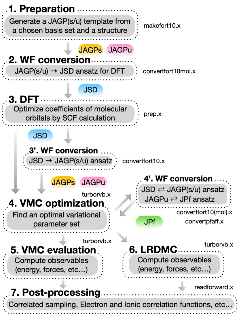
In recent years, there has been a surge of interest in materials informatics and digital transformation paradigms in the materials science community, which involve utilizing information science and computational chemistry/physics techniques to design or search for novel materials. The kernel method for high-throughput electronic structure calculations is most commonly the Density Functional Theory (DFT), which has been successfully used for designing various materials in silico [1, 2, 3, 4, 5, 6, 7, 8]. However, DFT sometimes loses the quantitative predictive power in particular cases, such as materials at extreme conditions or with strong electronic correlation [9, 10, 11, 12, 13, 14]. Instead, ab initio quantum Monte Carlo (QMC) does not lose predictive power even for such materials because it does not rely on any exchange-correlation functionals in its formalism [15]. However, when it comes to ab initio QMC applications, one of the biggest drawbacks is its complicated computational procedure. Indeed, a QMC study usually requires many involved operations, such as generating trial wave functions, variational optimizations, time-step or lattice-size extrapolation, and finite-size corrections. For instance, a typical workflow of a QMC calculation using the TurboRVB quantum Monte Carlo package [16, 17], is shown in Fig. 1. Automating such required tasks can offer a significant improvement in our productivity, enabling researchers to spend more time doing physics and chemistry rather than launching and monitoring jobs. So far, many workflow management packages have been developed to achieve a more productive research activity and high-throughput calculations. Some representatives are AiiDA [18], AFLOW [19], Fireworks [20], and  atomate [21], which have been widely used for generating and/or managing material science database such as NOMAD [22] and Materials Projects [23]. One could immediately exploit these established workflow systems also in QMC calculations, but the combination of a QMC code with these workflow packages is not straightforward due to the complexity of the QMC calculations. Thus, to manage them, we need to implement interfaces, if possible in Python, because most of the established workflow packages are also implemented based on Python, due to its appealing features. In fact, several packages for high-throughput QMC calculations, such as Nexus [24] and QMC-SW [25], are Python implementations. Wheeler et al. has very recently developed a new open-source Python-based package for real-space QMC, named PyQMC [26]. PyQMC is an all-Python package; thus, it enables one to develop algorithms and complex workflows more flexibly and user-friendly.

TurboGenius is an open-source Python package meant to manage TurboRVB calculations using a python script. In this paper, we explain the basic concepts, designs, functionalities, implemented classes, user interfaces, command-line tools of the package. TurboGenius provides Python classes and command-line tools that fully control TurboRVB jobs, which allow one to realize high-throughput QMC calculations. TurboGenius includes PyTurbo as a sub-package for providing users with more fundamental but more flexible building blocks to control TurboRVB jobs. For demonstrating high-throughput QMC calculations, we also implemented another open-source python package, TurboWorkflows. The demonstrations contain: (1) validations of DFT and QMC implementations of the TurboRVB package and (2) benchmarks of Diffusion Monte Carlo (DMC) calculations for several data sets. As per (1), we confirmed that DFT energies obtained by PySCF [27, 28] are consistent with those obtained by TurboRVB within the local density approximation (LDA), and Hartree-Fock (HF) energies obtained by PySCF and Quantum Package [29] are consistent with variational Monte Carlo (VMC) energies obtained by TurboRVB computed with the HF wavefunctions. The validation tests constitute a further reliability check of the TurboRVB package. As far as point (2) is concerned, we benchmarked atomization energies of the Gaussian-2 set [30], binding energies of the S22 [31], A24 [32], and SCAI [33] sets, and equilibrium lattice parameters of 12 cubic crystals. We found that, for all compounds analyzed in this study, the diffusion Monte Carlo (DMC) calculations with the LDA nodal surface give satisfactory results, i.e., consistent either with computational or with experimental reference values.

This paper is organized as follows: in Sec. II, we provide an overview of the TurboGenius program structure; in Sec. III, we provide an overview of the PyTurbo program structure; in Sec. IV, we describe the command-line tool and user interface implemented in TurboGenius; in Sec. V, we introduce TurboWorkflows, a python package for realizing high-throughput calculations using TurboGenius; and in Sec. VI, we showcase several validation and benchmark results obtained using TurboGenius and TurboWorkflows.

Figure 1: A typical workflow of a QMC calculation using TurboRVB; (1) Preparation of a JAGP(s/u) ansatz file from a chosen basis set, pseudo potentials, and a structure using makefort10.x binary. AGPs stands for the symmetric antisymmetrized geminal power (i.e., singlet correlation in the pairing function) [34], while AGPu stands for the broken symmetry antisymmetrized geminal power, (i.e., singlet + triplet correlations in the pairing function) [34]. The generated WF is a template, i.e., it is fulfilled with random numbers; thus, one needs to initialize it, typically using DFT; (2) Conversion of the generated JAGP(s/u) ansatz to JSD one using convertfort10mol.x binary because the subsequent DFT calculation works only with molecular orbitals (SD); (3) Initializing wave functions (WFs) using the build-in DFT module (prep.x); (3’) If one wants to use JAGP(s/u) ansatz, one can convert the initialized JSD ansatz to a JAGP(s/u) ansatz before the VMC optimization; (4) Optimization of a WF at the VMC level using turborvb.x binary; (4’) One can convert the optimized WF to another type of ansatz. Pf stands for the Pfaffian anstaz, which is the most general form of the AGP WF [17]. (5) Computation of observables such as energy and forces at the VMC level using turborvb.x binary; (6) Computation of observables such as energy and forces at the LRDMC level using turborvb.x; (7) Computation of other physical properties such as electron density.

II TurboGenius: Program overview

TurboGenius is implemented in Python 3 (the minimal requirement is Python 3.7). Python was chosen because it allows seamless integration with other major workflow frameworks. The main classes of TurboGenius are mainly composed of two types of classes. One is Wavefunction that stores and manipulates a wavefunction information including nuclear positions and pseudopotentials. The others are classes inheriting an abstract class (genius class). The classes enable one to control TurboRVB tasks, such as generating input files, launching jobs, and analyzing outcomes. The major classes of TurboGenius are listed in Table 1. Hereafter, we will describe the functionalities of the two main classes.

Table 1: Major classes of the TurboGenius package

Parent Class	Class (or Method)	Description
-	Wavefuntion	Manipulations and conversions of a TurboRVB WF file
Genius_IO	DFT_genius	Managing DFT calculations. The built-in program Prep is used.
	VMCopt_genius	Managing VMC optimizations.
	VMC_genius	Managing single-shot VMC calculations.
	LRDMC_genius	Managing single-shot LRDMC calculations.
	LRDMCopt_genius	Managing LRDMC optimizations.
	Correlated_sampling_genius	Managing correlated sampling jobs.

II.1 Wavefunction

Wavefunction is a class manipulating wavefunctions, such as for generating a JSD (Jastrow Slater Determinant) or JAGP (Jastrow correlated Antisymmetrized Geminal Power [16]) WF for a subsequent DFT initialization, and for converting a WF ansatz to another one (e.g., JSD to JAGP). The listing 1 shows a script to generate a WF file for the water molecule with the cc-pVQZ and cc-pVDZ basis sets for the determinant and the Jastrow parts, respectively, accompanied with the correlation consistent effective core potentials (ccECPs [35, 36, 37, 38]). The generated WF and PP files are fort.10 and pseudo.dat, respectively. Notice that Wavefunction currently has pre-defined keywords for correlation-consistent basis sets implemented in Basis Set Exchange [39] for all-electron calculations, and correlation-consistent effective core potentials (ccECPs) [35, 36, 37, 38] and Burkatzki-Filippi-Dolg (BFD) [40, 41] basis sets for pseudopotential calculations. One can also use different basis set and pseudopotentials by providing them as a text list. The generated WF is a Slater Determinant WF with randomized MO coefficients. Indeed, a user should initialize it using the built-in DFT (prep) code before doing QMC calculations.

The Wavefunction class also allows one to generate a wavefunction file from a TREXIO file [42]. The TREXIO library has a standard format for storing wave functions, together with a C-compatible API such that it can be easily used in any programming language, which is being developed in TREX (Targeting Real Chemical Accuracy at the Exascale) project [43]. The listing 2 shows a script to convert a TREXIO file. Thus, instead of using the built-in DFT program, prep, one can use standard quantum chemistry packages such as GAMESS [44] and PySCF [27, 28], then convert it to TurboRVB WF format. The class supports both all-electron and pseudopotential WF with/without periodic boundary conditions (i.e., for both molecules and crystals), and both restricted (ROHF) and unrestricted (UHF) open-shell WFs. Notice that a restricted WF is converted to the symmetric antisymmetrized geminal power (AGPs) (i.e., singlet correlation in the pairing function) [34], while an unrestricted WF is converted to the broken symmetry antisymmetrized geminal power (AGPu), (i.e., singlet + triplet correlations in the pairing function) [34].

Listing 1: A python script to generate a WF file

⬇

# import module

from turbogenius.wavefunction import Wavefunction

# generate a WF file from water.xyz

wavefunction = Wavefunction()

wavefunction.read_from_structure(

structure_file="water.xyz",

det_basis_set="cc-pVQZ",

jas_basis_set="cc-pVDZ",

pseudo_potential="ccECP",

)

wavefunction.to_jsd() # Jastrow-Slater WF.

Listing 2: A python script to read a TREXIO file

⬇

# import module

from turbogenius.wavefunction import Wavefunction

# Read a TREXIO File of water and convert

# it to the TurboRVB format.

wavefunction = Wavefunction()

wavefunction.from_trexio(

trexio_filename="trexio.hdf5"

)

wavefunction.to_jsd() # Jastrow-Slater WF.

wavefunction.to_jagps() # Jastrow-AGPs WF.

II.2 GeniusIO classes

GeniusIO is a parent class of the wrappers to manage complex QMC procedures. Several classes inheriting GeniusIO are implemented in TurboGenius, as shown in Table 1. Here, to make the explanation simple, we focus on one of the classes, VMC_genius. VMC_genius is a class to control VMC job of TurboRVB. The listing 3 shows a Python script to compute VMC energy of the hydrogen dimer.

Listing 3: A python script to compute VMC energy of the hydrogen dimer

⬇

# one needs "fort.10" (i.e., a WF file of the H2 dimer) for this calculation.

# import modules

from turbogenius.vmc_genius import VMC_genius

# (1) create a vmc_genius instance

vmc_genius = VMC_genius(

vmcsteps=600, # The number of MCMC steps

num_walkers=40, # The number of walkers

)

# (2) generate an input file

vmc_genius.generate_input(input_name="datas_vmc.input")

# (3) launch a VMC run

vmc_genius.run(input_name="datas_vmc.input", output_name="out_vmc.o")

# (4) compute energy and forces with reblocking

vmc_genius.compute_energy_and_forces(bin_block=10, warmupblocks=10)

# print vmc energy

print(f"VMC energy = {vmc_genius.energy:.5f} +- {vmc_genius.energy_error:.5f} Ha")

The procedure is composed of 4 steps, i.e., (1) create a vmc_genius instance, (2) generate an input file, (3) run the VMC job, and (4) post-processing (reblocking): (1) The input parameters used here are vmcsteps (int) and num_walkers (int) specifying the total number of Markov Chain Monte Carlo (MCMC) steps and the number of walkers used in total, respectively. (2) One can generage the input file corresponding to the parameters. (3) One can launch the VMC job. (4) After the VMC job is completed, one can post-process the outcomes depending on the type of jobs. For instance, in the VMC_genius class, the method compute_energy_and_forces allows one to get the means and variances of the energy, forces, and stresses using the TurboRVB built-in scripts implementing the bootstrap and jackknife methods [45], where one can use the reblocking (binning) technique to remove the autocorrelation bias.[46]. The related options are bin_block (int): block length and warmupblocks (int): the number of disregarded blocks.

The listing 4 shows a Python script to compute the VMC energy of the hydrogen dimer with JSD ansatz with DFT orbitals (JDFT). We notice that TurboRVB commands launched by TurboGenius can be specified through an environmental variable TURBOGENIUS_QMC_COMMAND. For instance, when one sets TURBOGENIUS_QMC_COMMAND=’mpirun -np 64 turborvb-mpi.x’, one can launch the VMC job with 64 MPI processes. One can run a serial job by an environmental value TURBOGENIUS_QMC_COMMAND=’turborvb-serial.x’.

Listing 4: A python workflow to obtain the VMC energy of the Hydrogen dimer.

⬇

#!/usr/bin/env python

# TREXIO -> JDFT WF (fort.10) -> VMCopt (only Jastrow) -> VMC (JDFT)

# import modules

import os, shutil

from turbogenius.pyturbo.basis_set import Jas_Basis_sets

from turbogenius.wavefunction import Wavefunction

from turbogenius.vmc_opt_genius import VMCopt_genius

from turbogenius.vmc_genius import VMC_genius

# trexio filename (Hydrogen dimer)

trexio_filename = "H2_trexio.hdf5"

# Start a workflow

root_dir = os.getcwd()

# TREXIO -> TurboRVB WF

trexio_dir = os.path.join(root_dir, "01trexio")

os.makedirs(trexio_dir, exist_ok=True)

shutil.copy(

os.path.join(root_dir, trexio_filename), os.path.join(trexio_dir, trexio_filename)

)

os.chdir(trexio_dir)

# Jastrow basis (GAMESS format)

H_jastrow_basis = """

S 1

1 1.873529 1.00000000

S 1

1 0.343709 1.00000000

S 1

1 0.139013 1.00000000

P 1

1 0.740212 1.00000000

"""

H2_jas_basis_sets = Jas_Basis_sets.parse_basis_sets_from_texts(

[H_jastrow_basis, H_jastrow_basis], format="gamess"

)

# convert the TREXIO file to the TurboRVB WF format (i.e., fort.10)

wavefunction = Wavefunction()

wavefunction.read_from_trexio(

trexio_filename=os.path.join(trexio_dir, trexio_filename),

jas_basis_sets=H2_jas_basis_sets,

)

os.chdir(root_dir)

# Optimization of Jastrow factor

vmcopt_dir = os.path.join(root_dir, "02vmcopt")

os.makedirs(vmcopt_dir, exist_ok=True)

copy_files = ["fort.10", "pseudo.dat"]

for file in copy_files:

shutil.copy(os.path.join(trexio_dir, file), os.path.join(vmcopt_dir, file))

os.chdir(vmcopt_dir)

# generate a vmcopt_genius instance

vmcopt_genius = VMCopt_genius(

vmcoptsteps=100,

steps=50,

warmupblocks=0,

num_walkers=40,

optimizer="lr",

learning_rate=0.35,

regularization=0.001,

opt_onebody=True,

opt_twobody=True,

opt_det_mat=False,

opt_jas_mat=True,

opt_det_basis_exp=False,

opt_jas_basis_exp=False,

opt_det_basis_coeff=False,

opt_jas_basis_coeff=False,

)

# generate the input file and run

vmcopt_genius.generate_input(input_name="datasmin.input")

vmcopt_genius.run(input_name="datasmin.input", output_name="out_min")

# average the optimized variational parameters

vmcopt_genius.average(optwarmupsteps=5)

os.chdir(root_dir)

# VMC calculation with the optimized WF

vmc_dir = os.path.join(root_dir, "03vmc")

os.makedirs(vmc_dir, exist_ok=True)

copy_files = ["fort.10", "pseudo.dat"]

for file in copy_files:

shutil.copy(os.path.join(vmcopt_dir, file), os.path.join(vmc_dir, file))

os.chdir(vmc_dir)

# generate a vmc_genius instance

vmc_genius = VMC_genius(

vmcsteps=300,

num_walkers=40,

)

# generate the input file and run

vmc_genius.generate_input(input_name="datasvmc.input")

vmc_genius.run(input_name="datasvmc.input", output_name="out_vmc")

# reblock the MCMC samples

vmc_genius.compute_energy_and_forces(bin_block=10, warmupblocks=5)

# VMC energy

energy, error = vmc_genius.energy, vmc_genius.energy_error

print(f"VMC-JDFT energy = {energy:.5f} +- {error:3f} Ha")

III PyTurbo: Program overview

PyTurbo is a sub-package of the TurboGenius package, which contains fundamental but flexible functionalities. The reason for implementing several classes in an independent sub-package is that there is a trade-off between flexibility and complexity (i.e., the availability of more sophisticated functionality). Indeed, we suppose advanced users will develop and exploit more elaborated procedures than the ones we expect at present. TurboGenius in its present status may not be flexible enough to support all of them. Therefore, we leave PyTurbo as an independent sub-package and keep its implementation as simple as possible, so that advanced users can be provided with the fundamental building blocks to fully control TurboRVB jobs in a Python environment. The major classes of PyTurbo are shown in shown in Table. 2. fort.10 is the most fundamental file containing all the WF information except for that of pseudo potentials. The information of pseudo potential is stored in a separate file, pseudo.dat. IO_fort10 and Pseudopotentials are classes for manipulating a WF file and PP files, respectively. PyTurbo contains several classes inheriting the abstract class fortranIO. They are essentially Fortran90 wrappers, i.e, in a one-to-one correspondence between a PyTurbo class and a TurboRVB Fortran binary (e.g., Makefort10 class in PyTurbo corresponds to makefort10.x in TurboRVB). The corresponding TurboRVB modules are listed in Table 3.

Table 2: Major classes of the PyTurbo package. Corresponding modules in TurboRVB are listed in Table 3.

Parent Class	Class	Description
-	IO_fort10	Represents many-body wavefunctions (i.e., fort.10). Allows wavefunction manipulations.
	Basis_sets	Represents basis sets.
	Pseudo_potentials	Represents pseudo potentials.
Fortran_IO	Makefort10	Python wrapper for a Fortran binary makefort10.x
	Convertfort10	Python wrapper for a Fortran binary convertfort10.x
	Convertfort10mol	Python wrapper for a Fortran binary convertfort10mol.x
	Convertpfaff	Python wrapper for a Fortran binary convertpfaff.x
	Prep	Python wrapper for a Fortran binary prep.x
	VMCopt	Python wrapper for a Fortran binary turborvb.x, tuned for VMC optimizations.
	VMC	Python wrapper for a Fortran binary turborvb.x, tuned for single-shot VMC calculations.
	LRDMCopt	Python wrapper for a Fortran binary turborvb.x, tuned for LRDMC optimizations.
	LRDMC	Python wrapper for a Fortran binary turborvb.x, tuned for single-shot LRDMC calculations.
	Readforward	Python wrapper for a Fortran binary readforward.x

Table 3: Main modules in TurboRVB [17].

Module	Description
makefort10.x	Generates a JSD/JAGP WF using a given basis set and structure.
convertfort10mol.x	Adds molecular orbitals. If the number of molecular orbitals is equal to (larger than) the half of the number of electrons in a system, the resultant WF becomes JSD (JAGPn).
convertfort10.x	Converts a JSD/JAGP/JAGPn WF to a JAGP one. It also converts an uncontracted atomic basis set to a hybrid (contracted) one using the geminal embedding scheme.
convertfortpfaff.x	Converts a JAGP WF to JPf one.
prep.x	Performs a DFT calculation.
turborvb.x	Performs VMC optimization, VMC evaluation, LRDMC, structural optimization and molecular dynamics.
readforward.x	Performs correlated samplings, and calculates various physical properties.

III.1 IO_fort10

IO_fort10 is a class to manipulate the TurboRVB WF file fort.10 and to extract particular information (e.g., the basis set for the determinant and the Jastrow parts). IO_fort10 internally uses the Basis_sets class that can store basis-set information for both the determinant and the Jastrow parts. Other information, such as lattice vectors, atomic positions, MO coefficients, AGP and Jastrow matrix elements, are stored in the corresponding attributes implemented in IO_fort10. The Atomic Simulation Environment (ASE) [47] package is used to read/write molecule and crystal structures for supporting various file formats.

III.2 Basis_sets

The Basis_sets class can store basis-set information for both the determinant and the Jastrow parts. TurboGenius supports the Gaussian-type localized atomic orbitals (GTOs):

$$\psi_{l,\pm m,I}^{{\text{Gaussian}}}\left({{\mathbf{r}};\zeta}\right)={\left|{{\mathbf{r}}-{{\mathbf{R}}_{I}}}\right|^{l}}{\operatorname{e}^{-\zeta{{\left|{{\mathbf{r}}-{{\mathbf{R}}_{I}}}\right|}^{2}}}}\cdot\Re[(-i)^{1\pm 1\over 2}{Y_{l,m,I}}\left({\theta,\varphi}\right)],$$ (1)

where the real and the imaginary part ($m>0$) of the spherical harmonic function ${Y_{l,m,I}}\left({\theta,\varphi}\right)$ centered at ${{{\mathbf{R}}_{I}}}$ are taken and rewritten in Cartesian coordinates in order to work with real defined and easy to compute orbitals, $l$ is the corresponding angular momentum and $m\geq 0$ is its projection number along the $z-$quantization axis. For the compatibility with TREXIO, the variables in the classes are defined in the exactly same way as in TREXIO. One can refer to the TREXIO documentation for the details [42]. The class also implements several parsers to write/read specific formats, such as GAMESS [48] and NWCHEM [49].

III.3 Pseudopotentials

Pseudopotentials class can store pseudopotential information. PyTurbo supports only the standard semi-local form

$$\hat{V}_{{\text{pp}}}^{I}\left({{{\mathbf{r}}_{i}}}\right)=V_{{\text{loc}}}^{I}\left({{r_{i,I}}}\right)+\sum\limits_{l=0}^{{l_{\max}}}V_{l}^{I}\left(r_{i,I}\right)\sum\limits_{m=-l}^{l}{\left|{{Y_{l,m}}}\right\rangle\left\langle{{Y_{l,m}}}\right|}$$ (2)

where $r_{i,I}=|{{\mathbf{r}}_{i}}-{{\mathbf{R}}_{I}}|$ is the distance between the $i$-th electron and the $I$-th ions, $l_{{\text{m}ax}}$ is the maximum angular momentum of the ion $I$, and $\sum\limits_{l=0}^{{l_{\max}}}{\sum\limits_{m=-l}^{l}{\left|{{Y_{l,m}}}\right\rangle\left\langle{{Y_{l,m}}}\right|}}$ is a projection operator on the spherical harmonics centered at the ion $I$. As it is now becoming a common practice not only in QMC, both the local $V_{{\text{loc}}}^{I}\left({{r_{i,I}}}\right)$ and the non-local $V_{l}^{I}\left(r_{i,I}\right)$ functions, are expanded over a simple Gaussian basis parametrized by coefficients (e.g., effective charge ${Z_{{\text{eff}}}}$ and other simple constants), multiplying simple powers of $r$, and a corresponding Gaussian term:

$${r^{2}}{V_{l}}\left(r\right)=\sum\limits_{k}{{\alpha_{k,l}}{r^{\beta_{k,l}-2}}\exp\left(-{{\gamma_{k,l}}{r^{2}}}\right)},$$ (3)

where ${{\alpha_{k,l}}}$, ${{\beta_{k,l}}}$ (usually small positive integers), and ${{\gamma_{k,l}}}$ are the parameters obtained by appropriate fitting. ${{\alpha_{k,l}}}$, ${{\beta_{k,l}}}$ and ${{\gamma_{k,l}}}$ are the parameters stored in the Pseudopotentials class. For the compatibility with TREXIO, the variables in the classes are defined in the exactly same way as in TREXIO. We refer to the documentation of TREXIO for the details [42].

III.4 Fortran90 wrappers

PyTurbo has several classes inheriting the fortranIO class, which are basically Fortran90 wrappers for the corresponding TurboRVB fortran binaries. The Listing 5 shows an example to compute the VMC energy of the Hydrogen dimer (assuming the optimized WF is given by a user) using PyTurbo. The input variable of VMC class is namelist instance that is an encapsulated dictionary with keys=fortran keyword and value=value of each parameter, as shown in Listing 5. Indeed, the input_parameters used in the Python script contains all parameters given to TurboRVB; thus, one can fully control TurboRVB jobs via PyTurbo.

Listing 5: VMC class in PyTurbo.

⬇

# pyturbo modules

from turbogenius.pyturbo.namelist import Namelist

from turbogenius.pyturbo.vmc import VMC

# input parameters of TurboRVB

input_parameters = {

"&simulation": {

"itestr4": 2,

"ngen": 5000,

"iopt": 1,

},

"&pseudo": {},

"&vmc": {},

"&readio": {},

"&parameters": {},

}

fortran_namelist = Namelist(namelist=input_parameters)

# Generate vmc instance with the above input parameters

vmc = VMC(namelist=fortran_namelist)

# VMC run

vmc.generate_input(input_name="datasvmc0.input")

vmc.run(input_name="datasvmc0.input", output_name="out_vmc0")

# VMC run (continuation)

vmc.set_parameter("iopt", 0)

vmc.generate_input(input_name="datasvmc1.input")

vmc.run(input_name="datasvmc1.input", output_name="out_vmc1")

# VMC, check if the jobs finished correctly

flags = vmc.check_results(output_names=["out_vmc0", "out_vmc1"])

# Reblock the MCMC samples

energy, error = vmc.get_energy(init=10, bin=10)

print(f"VMC energy = {energy:.4f} +- {error:.4f}")

IV Command-line tool and user interface

TurboGenius provides a useful command-line interface, named turbogenius_cli. The command-line tool can be run on a terminal by calling turbogenius, which is automatically installed during the setup procedure e.g., by pip. The command-line tool allows one to manipulate input and output files very efficiently and user-friendly. One of the most useful functions of the command-line tool is its helper, as shown in Listings 6 and 7. One can readily know what options are available and what each option does. This functionality is realized with the click package [50].

Listing 6: The helper implemented in TurboGenius.

⬇

% turbogenius --help

Usage: turbogenius [OPTIONS] COMMAND [ARGS]...

Options:

--help Show this message and exit.

Commands:

convertfort10 convertfort10_genius

convertfort10mol convertfort10mol_genius

convertpfaff readforward_genius

convertwf convert wavefunction

correlated-sampling correlated_sampling_genius

lrdmc lrdmc_genius

lrdmcopt lrdmcopt_genius

makefort10 makefort10_genius

prep prep_genius

vmc vmc_genius

vmcopt vmcopt_genius

Listing 7: The VMCopt helper implemented in TurboGenius.

⬇

% turbogenius vmcopt --help

Usage: turbogenius vmcopt [OPTIONS]

Options: (-g, -r, and/or -post is mandatory.)

-post Postprocess

-r Run a program

-g Generate an input file

-vmcoptsteps INTEGER Specify vmcoptsteps

-optwarmup INTEGER Specify optwarmupsteps

-steps INTEGER Specify steps per one iteration

-bin INTEGER Specify bin_block

-warmup INTEGER Specify warmupblocks

-nw INTEGER Specify num_walkers

-maxtime INTEGER Specify maxtime

-optimizer TEXT Specify optimizer, sr or lr

-learn FLOAT Specify learning_rate

-reg FLOAT Specify regularization

-opt_onebody flag for opt_onebody

-opt_twobody flag for opt_twobody

-opt_det_mat flag for opt_det_mat

-opt_jas_mat flag for opt_jas_mat

-opt_det_basis_exp flag for opt_det_basis_exp

-opt_jas_basis_exp flag for opt_jas_basis_exp

-opt_det_basis_coeff flag for opt_det_basis_coeff

-opt_jas_basis_coeff flag for opt_jas_basis_coeff

-twist flag for twisted average

-kpts INTEGER... kpts, Specify Monkhorst-Pack grids and shifts,

[nkx,nky,nkz,kx,ky,kz]

-plot flag for plotting graph

-log TEXT logger level, DEBUG, INFO, ERROR

--help Show this message and exit.

%

V TurboWorkflows: A python package for realizing high-throughput calculations using TurboGenius

Since TurboGenius is able to fully control TurboRVB jobs, one can implement workflows by combining it with a file/job managing package. To demonstrate it, as a proof of concept, we developed an open-source python package, TurboWorkflows, that enables one to compose simple workflows by combining TurboGenius with a job managing python package, TurboFilemanager. We notice that one can exploit other established workflow packages such as AiiDA [18] and Fireworks [20] as job-managing systems. Combining established workflow managers with TurboGenius is an intriguing future work. The main classes of TurboWorkflows are summarized in Table 4. Each workflow class inherits the parent Workflow class with options useful for a QMC calculation. For instance, in the VMC_workflow, one can specify a target accuracy (i.e., statistical error) of the VMC calculation. The VMC_workflow first submits an initial VMC run to a machine with the specified MPI and OpenMP processes to get a stochastic error bar per Monte Carlo step. Since the error bar is inversely proportional to the square root of the number of Monte Carlo samplings, the necessary steps to achieve the target accuracy is readily estimated by the initial run. The VMC_workflow then submits subsequent production VMC runs with the estimated necessary number of steps. Similar functionalities are also implemented in other workflow scripts such as VMCopt_workflow, LRDMC_workflow, and LRDMCopt_workflow. Figure LABEL:SI-fig:uml-vmc-workflow shows a Unified Modeling Language (UML) diagram of the VMC_workflow. The users can also define their own workflows inheriting the Workflow class.

TurboWorkflows can solve the dependencies of a given set of workflows and manage sequential jobs. The Launcher allows one to pass values and files obtained by a workflow to another workflow by using the Variable class, as shown in the listing 8. As shown in the listing 8, the Launcher class accepts workflows as a list, solves the dependencies of the workflows, and submits independent sequential jobs simultaneously. Launcher realizes this feature by the so-called topological ordering of a Directed Acyclic Graph (DAG) and the built-in python module, asyncio. The listing 8 shows a TurboWorkflows workflow script to perform a sequential job, PySCF $\rightarrow$ TREXIO $\rightarrow$ TurboRVB WF (JSD ansatz) $\rightarrow$ VMC optimization (Jastrow factor optimization) $\rightarrow$ VMC $\rightarrow$ LRDMC (lattice space $\rightarrow$ 0). Finally, we get the extrapolated LRDMC energy of the water dimer. Figure LABEL:SI-fig:uml-launcher shows the UML diagram corresponding to the script shown in the listing 8. If one wants to manipulate files or values in a more complex way, one should define a new workflow class inheriting the Workflow class and pass it into the Encapsulated_Workflow class.

Table 4: Major classes of the TurboWorkflows package.

Parent Class	Class	Description
-	Workflow	Abstract class for implementing workflows
	Encapsulated_Workflow	Encapsulated workflow class including input and output file handlings
	Launcher	A class for managing Encapsulated_Workflow instances, e.g., solving dependency.
Workflow	DFT_workflow	A workflow implementation based on DFT_genius
	VMC_workflow	A workflow implementation based on VMC_genius
	VMCopt_workflow	A workflow implementation based on VMCopt_genius
	LRDMC_workflow	A workflow implementation based on LRDMC_genius
	LRDMCopt_workflow	A workflow implementation based on LRDMCopt_genius
Workflow	PySCF_workflow	A workflow implementation based on PySCF
	TREXIO_workflow	A workflow implementation based on TREXIO

Listing 8: A python workflow to obtain the extrapolated LRDMC energy ($a\to 0$) of the water molecule.

⬇

#!/usr/bin/env python

# python packages

import os

import shutil

# turboworkflows packages

from turboworkflows.workflow_trexio import TREXIO_convert_to_turboWF

from turboworkflows.workflow_vmc import VMC_workflow

from turboworkflows.workflow_vmcopt import VMCopt_workflow

from turboworkflows.workflow_lrdmc_ext import LRDMC_ext_workflow

from turboworkflows.workflow_encapsulated import Encapsulated_Workflow

from turboworkflows.workflow_lanchers import Launcher, Variable

# dictionary of Jastrow basis (GAMESS format)

jastrow_basis_dict = {

"H": """

S 1

1 1.873529 1.00000000

S 1

1 0.802465 1.00000000

S 1

1 0.147217 1.00000000

""",

"O": """

S 1

1 1.686633 1.00000000

S 1

1 0.237997 1.00000000

S 1

1 0.125346 1.00000000

P 1

1 1.331816 1.00000000

""",

}

# Convert from a TREXIO file to a WF with TurboRVB format

trexio_workflow = Encapsulated_Workflow(

label="trexio-workflow",

dirname="trexio-workflow",

input_files=["water.hdf5"],

workflow=TREXIO_convert_to_turboWF(

trexio_filename="water.hdf5",

jastrow_basis_dict=jastrow_basis_dict,

),

)

# VMC optimization of Jastrow factor

# One-, two-, and three-body Jastrow are optimized

vmcopt_workflow = Encapsulated_Workflow(

label="vmcopt-workflow",

dirname="vmcopt-workflow",

input_files=[

Variable(label="trexio-workflow", vtype="file", name="fort.10"),

Variable(label="trexio-workflow", vtype="file", name="pseudo.dat"),

],

workflow=VMCopt_workflow(

# cluster information

cores=1,

openmp=1,

# vmc optimization, parameters

vmcopt_max_continuation=2,

vmcopt_num_walkers=40,

vmcopt_target_error_bar=7.5e-3,

vmcopt_trial_optsteps=10,

vmcopt_trial_steps=50,

vmcopt_production_optsteps=40,

vmcopt_optwarmupsteps_ratio=0.8,

vmcopt_bin_block=1,

vmcopt_warmupblocks=0,

vmcopt_optimizer="lr",

vmcopt_learning_rate=0.35,

vmcopt_regularization=0.001,

vmcopt_onebody=True,

vmcopt_twobody=True,

vmcopt_det_mat=False,

vmcopt_jas_mat=True,

vmcopt_det_basis_exp=False,

vmcopt_jas_basis_exp=False,

vmcopt_det_basis_coeff=False,

vmcopt_jas_basis_coeff=False,

vmcopt_maxtime=172000,

),

)

# VMC calculation with the optimized WF.

vmc_workflow = Encapsulated_Workflow(

label="vmc-workflow",

dirname="vmc-workflow",

input_files=[

Variable(label="vmcopt-workflow", vtype="file", name="fort.10"),

Variable(label="vmcopt-workflow", vtype="file", name="pseudo.dat"),

],

workflow=VMC_workflow(

# cluster information

cores=1,

openmp=1,

# vmc parameters

vmc_max_continuation=2,

vmc_num_walkers=40,

vmc_target_error_bar=5.0e-3,

vmc_trial_steps=150,

vmc_bin_block=10,

vmc_warmupblocks=5,

vmc_maxtime=172000,

),

)

# LRDMC calculations with the optimized WF

# LRDMC energies are computed with a = 0.20, 0.30, and 0.40, and then, extrapolated to a->0 limit.

lrdmc_ext_workflow = Encapsulated_Workflow(

label="lrdmc-ext-workflow",

dirname="lrdmc-ext-workflow",

input_files=[

Variable(label="vmc-workflow", vtype="file", name="fort.10"),

Variable(label="vmc-workflow", vtype="file", name="pseudo.dat"),

],

workflow=LRDMC_ext_workflow(

# cluster information

cores=1,

openmp=1,

# lrdmc, parameters

lrdmc_max_continuation=2,

lrdmc_num_walkers=40,

lrdmc_target_error_bar=5.0e-3,

lrdmc_trial_steps=150,

lrdmc_bin_block=10,

lrdmc_warmupblocks=5,

lrdmc_correcting_factor=10,

lrdmc_trial_etry=Variable(label="vmc-workflow", vtype="value", name="energy"),

lrdmc_alat_list=[-0.20, -0.30, -0.40, -0.50],

lrdmc_nonlocalmoves="tmove",

lrdmc_maxtime=172000,

),

)

# add the workflows to the Launcher class

cworkflows_list = [

trexio_workflow,

vmcopt_workflow,

vmc_workflow,

lrdmc_ext_workflow,

]

launcher = Launcher(cworkflows_list=cworkflows_list)

# Launch the jobs

launcher.launch()

VI Demonstrations of high-throughput calculations

In this section, we will show several results obtained using TurboGenius and TurboWorkflows. Earlier versions of TurboGenius was used for computing phonon dispersion calculations [51], equation of state calculations [51], potential energy surfaces of dimers [52, 53], binding energies of molecules [52, 53, 54], hydrogen liquids [55], and hydrogen solids [14]. However, they were not fully performed using a python script. The current versions of TurboGenius and TurboWorkflows allow one to fully control TurboRVB calculations using a python script. In this paper, we show two types of demonstrations, validations of the TurboRVB package and benchmarking QMC calculations using TurboRVB. The summary of the demonstrations are shown in Tables 5 and  6.

Table 5: Summary of the validation tests using TurboGenius and TurboWorkflows.

Data set	Target (TurboRVB)	Ref. (PySCF)	Purpose of the validation
38 molecules	LDA-DFT (prep)	LDA-DFT	Consistency check between the DFT module of PySCF and that of TurboRVB for open-boundary condition systems (molecules). The detail is written in Sec. VI.1.1.
10 crystals	LDA-DFT (prep)	LDA-DFT	Consistency check between the DFT module of PySCF and that of TurboRVB for periodic-boundary condition systems with insulating electronic states (without the smearing technique). $k$ = 4$\times$4$\times$4 was used. The detail is written in Sec. VI.1.1.
4 crystals	LDA-DFT (prep)	LDA-DFT	Consistency check between the DFT module of PySCF and that of TurboRVB for periodic-boundary condition systems with metallic electronic states (with the smearing technique). $k$ = 4$\times$4$\times$4 was used. The detail is written in Sec. VI.1.1.
100 molecules	VMC (turborvb)	RHF/ROHF	Consistency check between HF calculations done by PySCF and VMC calculations without Jastrow factor done by TurboRVB for open-boundary condition systems (molecules). RHF and ROHF were used for spin-unpolarized and spin-polarized systems, respectively. The same consistency check was done between TurboRVB and Quantum Package. The detail is written in sec. VI.1.2.
49 molecules	VMC (turborvb)	UHF	Consistency check between HF calculations done by PySCF and VMC calculations without Jastrow factor done by TurboRVB for open-boundary condition systems (molecules) with spin-polarized states (UHF was used). The detail is written in Sec. VI.1.2.
9 crystals	VMC (turborvb)	RHF/ROHF	Consistency check between HF calculations done by PySCF and VMC calculations without Jastrow factor done by TurboRVB for periodic-boundary condition systems. RHF and ROHF were used for spin-unpolarized and spin-polarized systems, respectively. $k$ = $\Gamma$, $k$ = (0.25, 0.25, 0.25), and $k$ = 4$\times$4$\times$4 were tested. The detail is written in Sec. VI.1.2.

Table 6: A summary of the benchmarks using TurboGenius and TurboWorkflows.

Data set	Description of the benchmark test
G2-set	Benchmarking the atomization energies of 55 molecules. They were computed using LRDMC at the $a\rightarrow 0$ limit. The JSD ansatz with the LDA-PZ nodal surface was employed. The references are experimental values. The detail is written in Sec. VI.2.1.
S22-set	Benchmarking the binding energies of 22 complex systems. They were computed using LRDMC at the $a\rightarrow 0$ limit. The JSD ansatz with the LDA-PZ nodal surface was employed. The references are CCSD(T) values. The detail is written in Sec. VI.2.1.
A24-set	Benchmarking the binding energies of 24 complex systems. They were computed using LRDMC at the $a\rightarrow 0$ limit. The JSD ansatz with the LDA-PZ nodal surface was employed. The references are CCSD(T) values. The detail is written in Sec. VI.2.1.
SCAI-set	Benchmarking the binding energies of 24 complex systems. They were computed using LRDMC at the $a\rightarrow 0$ limit. The JSD ansatz with the LDA-PZ nodal surface was employed. The references are CCSD(T) values. The detail is written in Sec. VI.2.1.
CO dimer	Benchmarking the equilibrium bond length and harmonic vibrational frequency of the CO dimer. They were estimated from potential energy surfaces with the JSD (LDA-PZ nodal surface) and JAGP ansatz. The references are experimental values. The details is written in Sec. VI.2.2.
Cubic crystals	Benchmarking the equilibrium lattice parameters 12 cubic crystals. They were estimated by fitting the equation of states obtained by LRDMC. The JSD ansatz with the LDA-PZ nodal surface was employed. The references are experimental values. The detail is written in Sec. VI.2.3.

VI.1 Validations of QMC implementations

Validation of scientific softwares, such as checking consistency among softwares that implement the same theory as employed in this study (i.e., inter-software test), is an important step to ensure one’s software reliability. The widespread use of validation tests is also important to ensure the trustability of numerical simulations in general. Such validation tests have been performed not-so-widely in the ab initio QMC community, since QMC requires complex computational procedures, as mentioned in the introduction. TurboGenius and TurboWorkflows enable one to do the tests much more easily and efficiently. In this paper, we report the results of inter-software tests for the TurboRVB package (v1.0.0). We checked inter-package consistencies between TurboRVB and other established quantum chemistry packages, such as PySCF [27, 28] and Quantum Package [29]. The details are written in Secs. VI.1.1 and  VI.1.2. Notice that the data and Python scripts to reproduce the validation tests are available from our public repositories (see Sec. VIII).

VI.1.1 Validation of DFT module: LDA (PySCF) v.s. LDA (TurboRVB-prep)

Using the implemented workflows, we have checked the consistency of the DFT-LDA calculations among packages. DFT energies should be consistent among packages as far as the same basis sets and ECPs are used even though those DFT codes employ different implementation schemes. For the reference calculations, we used the PySCF package (v2.0.1) [27, 28] with the Perdew-Zunger (PZ81) local density approximation (PZ-LDA) [56]. For the test sets, we have chosen (1) 38 molecules with singlet spins, (2) 10 insulating crystals, where both orthorhombic and non-orthorhombic cells are included, and (3) 4 metallic crystals. For the crystals, we employed the $k$ = 4 $\times$ 4 $\times$ 4 (i.e., twisted average) grid such that the reciprocal grid includes both real and complex points. For the real-space grid, which is needed for the numerical integration employed in the built-in DFT module (prep), we employed 0.05 Bohr for the molecules and insulating crystals, while 0.03 Bohr for the metallic crystals. We employed the Fermi-Dirac smearing method with 0.01 Ha for the metals. Figures. LABEL:SI-fig:sanity-check-molecules-LDA, LABEL:SI-fig:sanity-check-crystals-LDA-pbc-kgrid-insulator, and LABEL:SI-fig:sanity-check-crystals-LDA-pbc-kgrid-metal show the consistencies between PySCF and TurboRVB-prep LDA calculations for all the above cases. The very slight differences come from the implementations (i.e., TurboRVB-prep module employs the numerical integration to compute the overlap and Hamiltonian matrix elements). The corresponding numbers are shown in Tables. LABEL:SI-tab:sanity-check-molecules-LDA, LABEL:SI-tab:sanity-check-crystals-LDA-pbc-kgrid-insulator, and LABEL:SI-tab:sanity-check-crystals-LDA-pbc-kgrid-metal. The consistencies between the packages show that the implementations of DFT calculations in the TurboRVB package is correctly done.

VI.1.2 Validation of TurboRVB QMC module: HF (PySCF) v.s. VMC (TurboRVB w/o Jastrow)

One of the most prominent features of TurboGenius is the functionality to convert a TREXIO file to a TurboRVB WF because it allows one to use any quantum chemistry or DFT packages to generate trial WFs as long as they employ localized basis sets. We have carefully verified the implementation of the converter by confirming the consistency between HF and VMC energies without Jastrow factor, both for molecules (open systems) and crystals (periodic systems). More specifically, we computed the HF energies of 100 molecules and 9 crystals (such that both orthorhombic and non-orthorhombic cells are included) by PySCF v2.0.1, where the ccECP [35, 36, 37, 38] with accompanied basis sets were employed. The obtained PySCF checkpoint files were converted to TurboRVB WFs via TREXIO files using the converter implemented in TurboGenius package. Then, we computed VMC energies of the TurboRVB WFs without Jastrow factor. The PySCF to TurboRVB conversion via TREXIO supports both restricted (i.e., ROHF) and unrestricted (i.e., UHF) open-shell WFs. We tested the former implementation using the 100 molecules, while the latter using the 49 molecules. For the 100 molecules, the same consistency checks were done between HF calculations by Quantum Package (v2.1.2) and TurboRVB. For the crystals, we tested both single-$k$ and multi-$k$ (i.e., twisted average) calculations. For the single-$k$ tests, $k$=(0.00, 0.00, 0.00) and (0.25, 0.25, 0.25) were used. For the twisted average tests, we employed $k$ = 4 $\times$ 4 $\times$ 4 such that the grid includes both real and complex points. Notice that, in the twisted average case, we compared the VMC energies with the averages of the HF energies obtained at each $k$-point independently, since the VMC is independently done for each $k$ point (i.e., MCMC is done for each $k$.) We did not use metals for the VMC validation tests. This is because, for metals, the HF energy obtained with the smearing technique is not consistent with the VMC ones due to the fact that the orbital contributions above the Fermi energy are truncated when converting the DFT orbitals to the single Slater-Determinant ansatz. The HF and VMC energies should be consistent within the statistical errors (i.e., within $3\sigma$) as long as the conversions are done correctly. The results of the validation tests are shown in Figs.LABEL:SI-fig:sanity-check-molecules-RHF-LABEL:SI-fig:sanity-check-crystals-k-twist. The corresponding values are shown in Tables LABEL:SI-tab:sanity-check-molecules-RHF-LABEL:SI-tab:sanity-check-crystals-k-twist. The results show that the HF and VMC energies are consistent within the statistical errors (i.e., within $3\sigma$), implying that the implementations of the WF converter and VMC calculations in the TurboRVB package are correctly done.

VI.2 Benchmarking of QMC calculations

Benchmarking a theory with several typical systems is a task as important as the validation test, with the aim at examining the accuracy of the theory. Such benchmark calculations can also be performed efficiently using TurboGenius and TurboWorkflows. In this work, we benchmarked atomization energies of the Gaussian-2 set [30], binding energies of the S22 [31], A24 [32], and SCAI [33] sets, and equilibrium lattice parameters of 12 crystals via equation of states calculations. We found that, for all the compounds, the diffusion Monte Carlo calculations with the PZ-LDA nodal surface give satisfactory results, i.e., consistent either with CCSD(T) or experimental values. The details of the results are reported in the following parts.

VI.2.1 G2, S22, A24, and SCAI benchmark sets: atomization energy and binding energy calculations

We report the result of the benchmark tests using the G2 [30], S22 [31], A24 [32], and SCAI [33] sets. The G2-set targets atomization energies of 55 molecules, while the other sets benchmark binding energies of complex systems. The benchmark calculations were performed by TurboWorkflows. Our python workflow launched a sequential job for each atom and molecule, PySCF $\rightarrow$ TREXIO $\rightarrow$ TurboRVB WF (Jastrow Slater determinant ansatz) $\rightarrow$ VMC optimization (Jastrow factor) $\rightarrow$ VMC $\rightarrow$ LRDMC (lattice space $\rightarrow$ 0). Finally, we got extrapolated LRDMC energies of atoms and molecules of the benchmark sets. The quality of the Jastrow optimization did not affect the final extrapolated LRDMC energy because the determinant localization approximation (DLA) [57] was employed. Indeed, the workflow was fully automatic and fully reproducible since the determinant part which determines the nodal surface was obtained deterministically, and the Jastrow factor, which was obtained by stochastic optimization, did not affect the extrapolated FN energy. The geometries of the G2 set were taken from previous benchmark studies [58, 59, 60], while those of the other dataset were taken from Benchmark Energy and Geometry DataBase (BEGDB) [61]

Figure 2: Deviation of the LRDMC atomization energies obtained in this study from the experimentally obtained values. Corrections for zero-point energies and relativistic effects have been included before computing the differences between the LRDMC and experimental values [62]. The blue and red bounds represent discrepancies $\pm$ 5 kcal/mol and $\pm$ 1 kcal/mol, respectively. DFT calculations with PZ-LDA [56] exchange-correlation functional were used to generate the trial WFs. The cc-pVQZ basis set with the accompanied ccECP pseudo potentials [35, 36, 37, 38] were employed for the DFT calculations.

Figure 3: The binding energy comparison of the S22 benchmark set. The differences between the LRDMC values obtained in this study and the reference CCSD(T) values are plotted. The blue and red bounds represent discrepancies $\pm$ 5 kcal/mol and $\pm$ 1 kcal/mol, respectively. DFT calculations with PZ-LDA [56] exchange-correlation functional were used to generate the trial WFs. The cc-pVQZ basis set with the accompanied ccECP pseudo potentials [35, 36, 37, 38] were employed for the DFT calculations.

Figure 4: The binding energy comparison of the A24 benchmark set. The differences between the LRDMC values obtained in this study and the reference CCSD(T) values are plotted. The blue and red bounds represent discrepancies $\pm$ 5 kcal/mol and $\pm$ 1 kcal/mol, respectively. DFT calculations with PZ-LDA [56] exchange-correlation functional were used to generate the trial WFs. The cc-pVQZ basis set with the accompanied ccECP pseudo potentials [35, 36, 37, 38] were employed for the DFT calculations.

Figure 5: The binding energy comparison of the SCAI benchmark set. The differences between the LRDMC values obtained in this study and the reference CCSD(T) values are plotted. The blue and red bounds represent discrepancies $\pm$ 5 kcal/mol and $\pm$ 1 kcal/mol, respectively. DFT calculations with PZ-LDA [56] exchange-correlation functional were used to generate the trial WFs. The cc-pVQZ basis set with the accompanied ccECP pseudo potentials [35, 36, 37, 38] were employed for the DFT calculations.

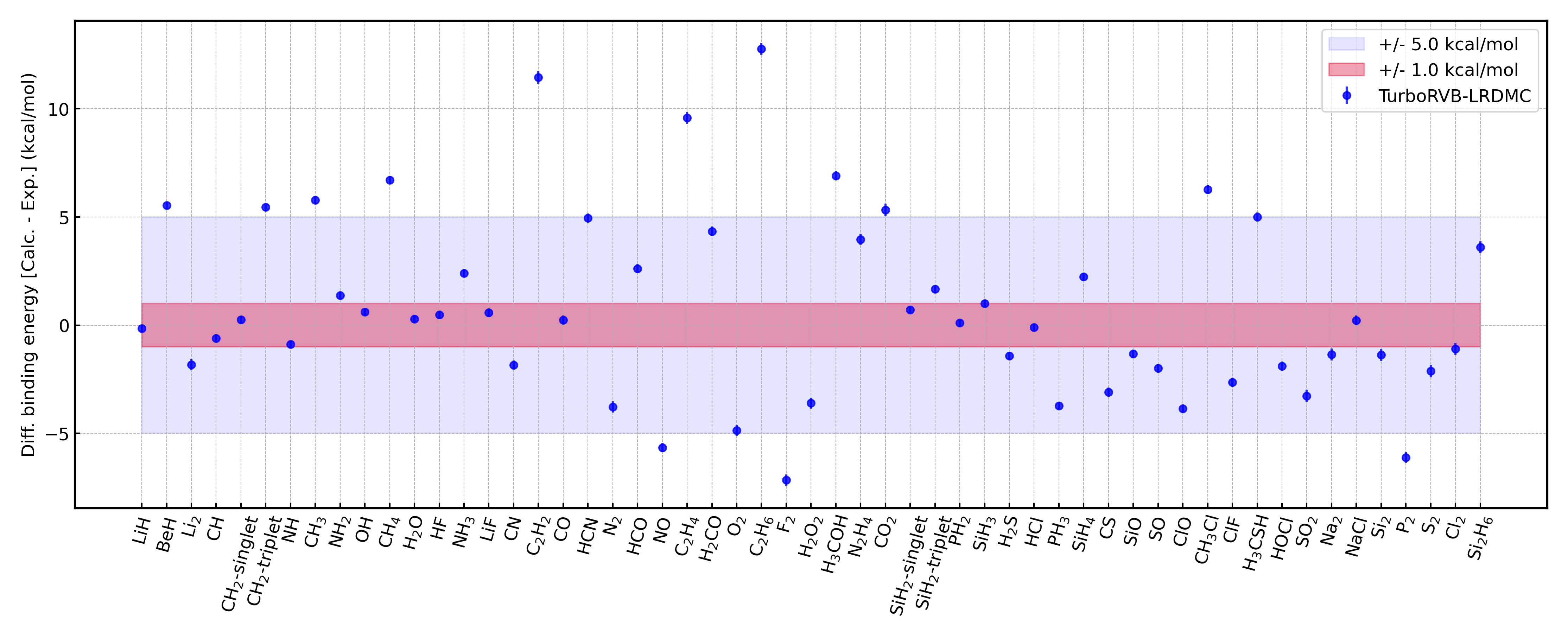
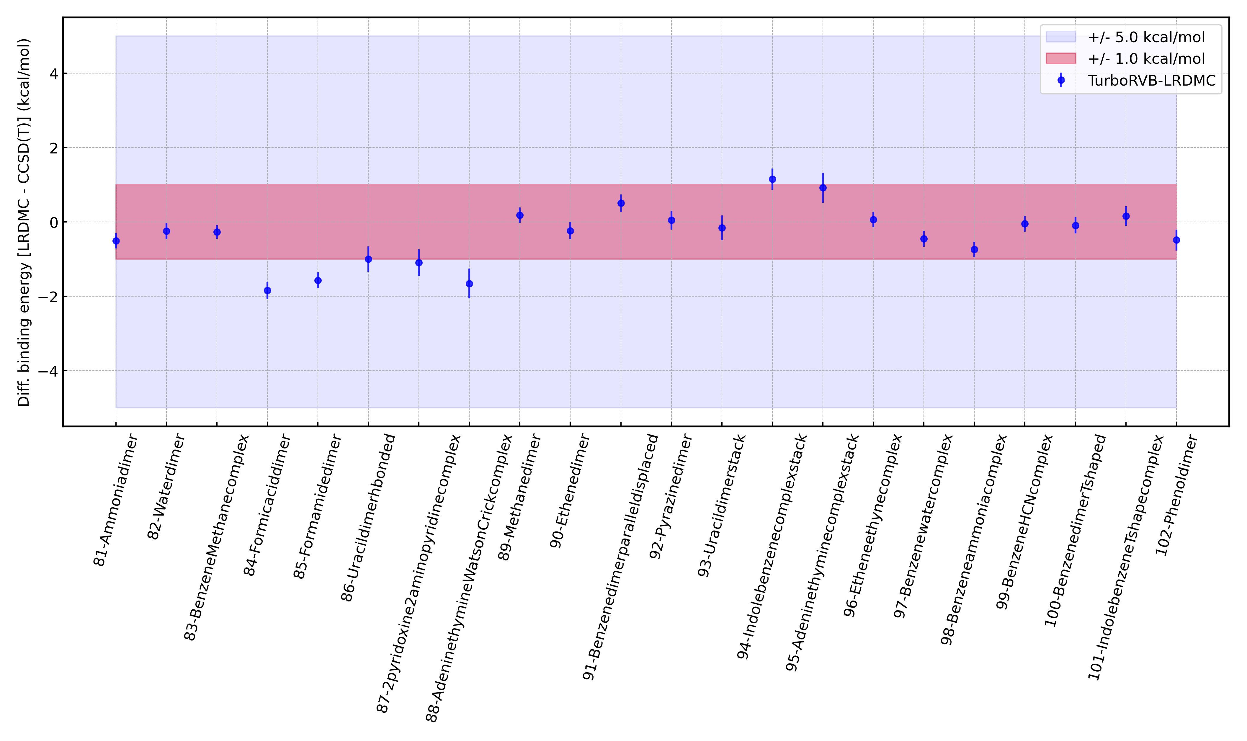
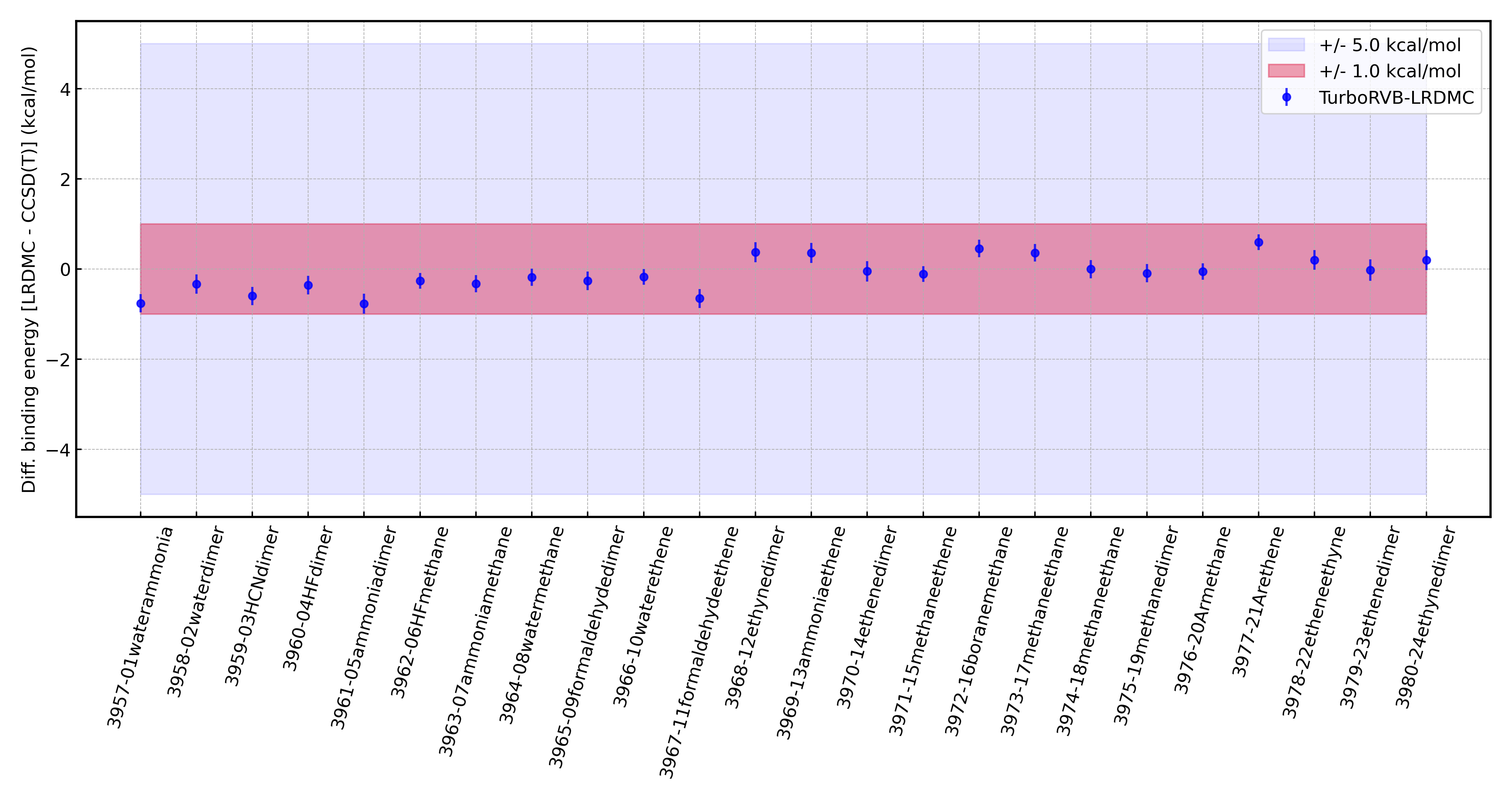
Figure. 2 shows the benchmark result for the G2-set [30]. The corresponding numbers are shown in Table LABEL:SI-tab:G2-set. We computed the atomization energies of the 55 molecules included in the G2-set by pseudo-potential LRDMC calculations with the JDFT ansatz. We employed the cc-pVQZ basis set with the accompanied ccECP [35, 36, 37, 38] pseudo potentials. For the DFT calculations, we used the PySCF package (v2.0.1) [27, 28] with PZ-LDA [56] exchange-correlation functional. The obtained Mean absolute deviation (MAD) with the JDFT ansatz is 3.242 kcal/mol, which is consistent with previous studies. Nemec et al. [62] used all-electron DMC on Slater determinant (SD) WF to obtain the binding energies of the G2 set to an MAD of 3.2 kcal/mol. Grossman [63] reported a similar accuracy, a MAD of 2.9 kcal/mol, in binding energies by DMC pseudopotential calculations. Abhishek et al. [54] reported a MAD of 3.2 kcal/mol by all-electron LRDMC calculations with the JDFT ansatz. Recently, Abhishek et al. [54] also reported a MAD of 1.6 kcal/mol by all-electron LRDMC calculations with the JAGPs ansatz. TurboGenius and TurboWorkflows support the same binding energy calculations with the JAGP ansatz also. However, to reproduce their results, large Jastrow basis sets and very careful optimizations are needed; otherwise, optimizations could be stuck at local mimina. The fully automatic optimization of WFs with many variational parameters is not established yet. This should be solved in the near future for realizing robust high-throughput QMC calculations with optimized (beyond-DFT) nodal surfaces.

The S22 dataset was developed by Hobza et al. for testing interaction energies for small complex systems [31]. Figure. 3 shows the benchmark result for the S22-set. The corresponding numbers are shown in Tab. LABEL:SI-tab:S22-set. We employed the cc-pVQZ basis set with the accompanied ccECP [35, 36, 37, 38] pseudo potentials. For the DFT calculations, we used the PySCF package (v2.0.1) [27, 28] with PZ-LDA [56] exchange-correlation functional. The obtained MAD is 0.610 kcal/mol. A subset of the S22-benchmark was studied by Dubecky et. al. [64, 65]. They extracted a subset of the S22 benchmark test, ammonia dimer, water dimer, methane dimer, ethene dimer, ethene–ethyne, benzene–water, benzene–methane, and benzene dimer (T-shape). They employed the ECPs with the corresponding basis sets (aug-TVZ) developed by Burkatzki et al. [40]. They used the B3LYP exchange-correlation functional for generating the trial wave functions. Their obtained binding energies, -3.10(6), -5.15(8), -0.44(5), -1.47(9), -1.56(8), -3.53(13), -1.30(13), and -2.88(16) kcal/mol are very closed to ours, -3.68(21), -5.26(21), -0.35(20), -1.75(23), -1.47(20), -3.73(21), -1.77(18) and -2.83(22) kcal/mol for ammonia dimer, water dimer, methane dimer, ethene dimer, ethene–ethyne, benzene–water, benzene–methane, and benzene dimer (T-shape), respectively. The full set of the S22-benchmark was studied by Korth et. al. [66]. They used the guidance functions of the Slater-Jastrow type with Hartree-Fock determinants and Schmidt-Moskowitz type correlation functions. [67]. They used quadruple $\zeta$ valence GTO basis sets fully optimized for the ECPs developed by Ovcharenko et al. [68]. Their obtained MAD (0.68 kcal/mol) is very close to ours (0.61 kcal/mol).

The A24 dataset is a set of non-covalent systems large enough to include various types of interactions [32]. The dataset was intended for testing accuracy of computational methods which are used as a benchmark in larger model systems. Figure. 4 shows the benchmark result for the A24-set. The corresponding numbers are shown in Table LABEL:SI-tab:A24-set. We employed the cc-pVQZ basis set with the accompanied ccECP [35, 36, 37, 38] pseudo potentials. For the DFT calculations, we used the PySCF package (v2.0.1) [27, 28] with PZ-LDA [56] exchange-correlation functional. The obtained MAD is 0.315 kcal/mol. The full set of the A24-benchmark was studied by Dubecky et. al. [65]. They investigated the effects of the basis set, Jastrow factor, and optimization protocols. They finally obtained MAD of 0.15 kcal/mol with the single-determinant trial wave functions of Slater-Jastrow type using B3LYP orbitals and aug-TZV basis sets accompanied with the ECPs developed by Burkatzki et al. [40]. Their MAD (0.15 kcal/mol) is very closed to the value reported in this study (0.315 kcal/mol).

The SCAI dataset is developed to benchmark interactions between amino acid side chains [33]. The dataset contains a representative set of 24 of the 400 (i.e., 20 $\times$ 20) possible interacting side chain pairs. Figure. 5 shows the benchmark result for the SCAI-set. The corresponding numbers are shown in Table. LABEL:SI-tab:SCAI-set. We employed the cc-pVQZ basis set with the accompanied ccECP [35, 36, 37, 38] pseudo potentials. For the DFT calculations, we used the PySCF package (v2.0.1) [27, 28] with PZ-LDA [56] exchange-correlation functional. The obtained MAD is   0.402 kcal/mol, which is as small as the S22 and A24 benchmark sets. To the best of our knowledge, no one has benchmarked the SCAI data set using QMC. Among the systems, 704-DH1 and 705-DHN1 show the largest deviations, -1.33(26) kcal/mol and -2.15(26) kcal/mol, respectively.

VI.2.2 Potential Energy Surface (PES) calculations

Potential Energy Surface (PES) calculations are often computed for dimers in QMC for benchmarking, i.e., for comparing binding energies, equilibrium bond lengths, and harmonic frequencies with experimental values, and for checking if the obtained forces and pressures are biased or not [69, 70, 34, 71, 72, 53, 73]. To reduce the computation costs of PES calculations and avoid being trapped at local minima, Jastrow factors are usually optimized at a certain bond length and copied to WFs with other bond lengths which will then be optimized with a better starting point. TurboWorkflows automatizes these procedure and, for a good point, solves the dependency automatically. An example workflow is shown in Listing LABEL:SI-lst:turboworkflows-CO-workflow, where the initial Jastrow optimization procedure is defined for a bond length (1.10 Å) and the optimized Jastrow factors are copied to WFs at other bond lengths and optimized again. The point is the Value instance that defines workflows that should be completed before. The workflow for the PES calculation is showin in Fig. 7. The PESs were computed at both the VMC and LRDMC levels. Two ansatz were employed in this study, JDFT and JAGPs. The JDFT ansatz were optimized according to the procedure described above using the linear method [74] at the VMC level and then they were converted to the JAGPs ansatz. The JAGPs were further optimized using the linear method at the VMC level. The optimized JDFT and JAGP ansatz were used for the subsequent LRDMC calculations. The T-move approach [75] with the lattice discretization = 0.30 Bohr was employed for the LRDMC calculations. The obtained PESs are shown in Fig. 6. The left-hand side of Fig. 6 shows that the PESs obtained with JDFT and JAGPs ansatz at the VMC level, while the righthand of Fig. 6 shows that the PESs obtained with JDFT and JAGPs ansatz at the LRDMC level. Table 7 summarizes the equilibrium bond length and the harmonic frequency obtained from the VMC and LRDMC calculations and those obtained from experiments. The LRDMC calculation with the JAGPs ansatz gives the closest values to the experiment, as expected. The remaining discrepancies can be solved using a larger determinant and Jastrow basis sets as they both affect the quality of the nodal surfaces. Such a benchmark test for other molecules is an intersting future work. The workflow will be also useful for benchmarking new ansatz and algorithms implemented in TurboRVB.

Figure 6: PESs of the CO dimer computed by a python workflow implemented using TurboWorkflows. The left and right PESs were computed at the VMC and LRDMC levels, respectively. The green and blue vertical broken lines represent the equilibrium distances obtained from the JSD (with the LDA-PZ nodal surface) and JAGP PESs, respectively. The red vertical broken line shows the experimental equilibrium distance.

Figure 7: Dependencies of the PES calculation for the CO dimer. The dependencies are automatically solved by the launcher implemented in TurboWorkflows.

Table 7: Equilibrium bond distances $r_{\rm eq}$ (Å) and harmonic frequencies $\omega$ (cm^-1) of the CO dimer obtained with the JDFT and JAGPs ansatz both at the VMC and LRDMC levels.

Method	Ansatz	$r_{{\rm eq}}$ (Å)	$\omega$ (cm-1)
VMC	JDFT	1.1150(2)	2272(3)
	JAGPs	1.1186(2)	2233(3)
LRDMC	JDFT	1.1223(2)	2212(3)
	JAGPs	1.1240(2)	2194(3)
Exp.	-	1.128323	2169.81358

VI.2.3 Benchmarking Equations of State in Solids

We report the Equation of States (EOSs) of 12 solids computed at the VMC and LRDMC levels by TurboWorkflows. Such a benchmark has been done for several crystals to test the accuracy of QMC calculations [77, 78]. Table 8 shows the Crystallography Open Database(COD)-IDs [79, 80] of the 12 crystals computed in this demonstration. The 12 crystals were chosen because Ref. 81 summarizes experimental lattice parameters at 0 K with the zero-point energy subtracted, which are directly comparable with our results.

First of all, we carefully checked the basis-set convergence since PySCF, which generates trial wavefunctions for the subsequent TurboRVB calculations, employs the localized basis set also for the periodic systems. In other words, the convergence is sometimes difficult to be achieved unlike the plane-wave one. To check the basis-set convergence, we compared the EOSs of the 12 crystals obtained by PySCF (localized basis-set) and QuantumEspresso (Plane-Wave basis set with a 800 Ryd cutoff) with the same ccECP pseudopotentials [35, 36, 37, 38]. The basis set convergence check using 1$\times$1$\times$1 supercell is shown in Fig. LABEL:SI-fig:eos-basis-check-s-1-1-1 and the finally chosen basis sets are listed in Table 8. We found that, to achieve the convergence, a large basis set (e.g., V5Z) is often needed. Notice that, in the localized basis sets, orbitals whose exponent is smaller than 0.10 were cut to avoid the numerical instability (i.e., linear-dependency [51]). The consistency holds also for the 2$\times$2$\times$2 supercells as shown in Fig. LABEL:SI-fig:eos-basis-check-s-2-2-2. The slow convergence with respect to the basis set size comes from the fact that the provided basis sets were tuned using molecules, not solids. Indeed, the exponents are not suitable for solids. Therefore, to achieve a better convergence, we recommend to use basis sets optimized for solids [82].

We have confirmed that the 2$\times$2$\times$2 supercell with $k$=2$\times$2$\times$2 twisted average is large enough to mitigate the one-body finite size effect for Diamond (Fig. LABEL:SI-fig:eos-onebody-check-diamond). It should be common among all the compounds we are studying because they are all insulators with similar lattice parameters. We have not checked whether 2$\times$2$\times$2 supercells are large enough to mitigate the two-body error, but we can assume so because the EOS calculations depend on the relative energies. In fact, Ref. 83 shows that larger supercells do not change the lattice parameter.

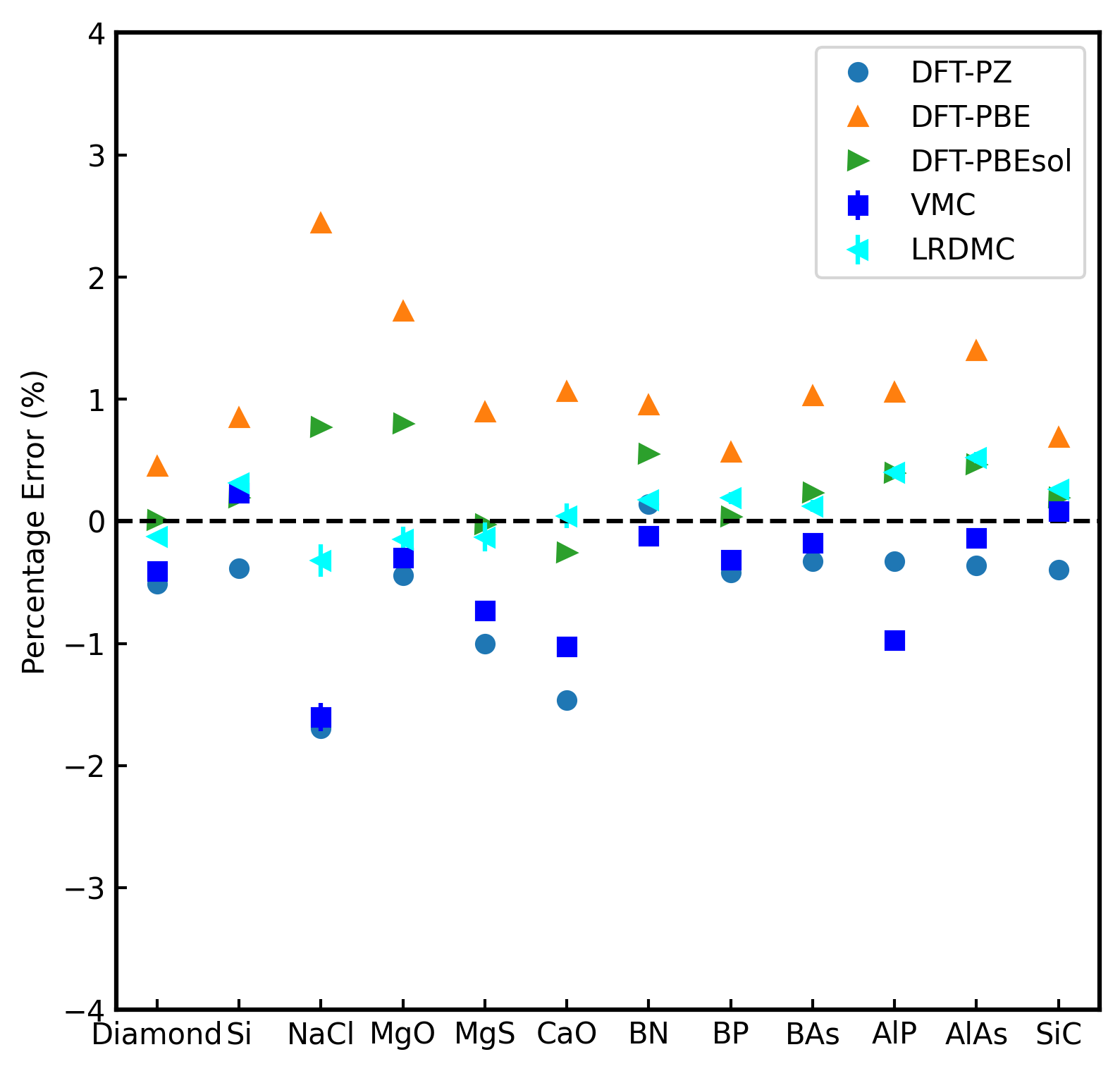
Figure 8 shows the EOSs of the 12 crystals computed at the VMC and LRDMC levels with the LDA-PZ nodal surfaces with the converged basis sets. The DFT calculations with the XC=LDA-PZ [56], PBE [84], and PBEsol [85] were performed using Quantum Espresso with the Ultra-soft PPs provided by the PS-library Project (v.1.0.0) [86]. The 2$\times$2$\times$2 supercells and $k$=2$\times$2$\times$2 meshes were employed for all the calculations. The obtained PESs were fitted by the Vinet function [87]. Table 8 shows the lattice parameters ($a_{0}$) obtained from the Vinet fittings and the available experimental values [81]. We evaluated the performance of the methods by mean absolute error (MAE: $\frac{1}{M}(\Sigma{|a_{\rm calc.}-a_{\rm exp.}|})$) and mean absolute relative error (MARE: $\frac{1}{M}(\Sigma{\frac{|a_{\rm calc.}-a_{\rm exp.}|}{a_{\rm exp.}}}\times 100)$), where $M$ is the sample size (i.e., $M=12$ in this work). Fig. 9 shows percentage errors in the calculated lattice parameters compared to experimental ones.

On one hand, our results show that the accuracy of the VMC calculations on the lattice parameter is strongly dependent on crystals. For instance, the estimated equilibrium lattice parameter of Diamond is well consistent with the experimental value both at the DFT and VMC levels, while that of NaCl was severely underestimated. The MARE for the VMC calculations is 0.5087(75) %, which is slightly better than that for the DFT-LDA calculations, while worse than that of the DFT-PBEsol calculations. The results imply the VMC calculations (with the small Jastrow factor employed in this study) is sometimes not sufficient to get accurate EOSs.

On the other hand, our results show that the DMC calculations with the LDA-PZ nodal surfaces are much less dependent on the choices of XCs for generating the trial wave functions, showing the accuracy of the methods. The conclusion is in line with the benchmark calculations presented in Refs. 77 and  78, showing that DMC is highly accurate in describing the structural properties of a broad range of solids and that these structural properties are rather insensitive to the given nodal surfaces. The MARE for the DMC calculations is 0.229(11) %, which is the best result among the methods tested in this study. The remaining discrepancy between the experiments and calculations could come either from the fixed nodal surface (i.e., the LDA-PZ is used in this study), from the qualities of the PPs (ccECP), or from their related non-local properties (i.e., in case of T-moves, the quality of the Jastrow factor can still affect the results). In these regards, more comprehensive benchmark tests on the EOS calculations using TurboWorkflows will be an interesting perspective.

Figure 8: Results of the equation of state calculations for the 12 crystals by DFT, VMC, and LRDMC. The dot points are obtained values, and the solid lines are the curves obtained by a fit of the Vinet equation to calculations. The VMC and DMC points have statistical errors. In the plots, the error bars represent 2$\sigma$. The experimental equilibrium volumes and those obtained by a fit of the Vinet equation to calculations are plotted as vertical broken lines. Notice that the finite temperature thermal expansion and zero point energy were corrected in the experimental values [81].

Figure 9: Percentage errors in the obtained lattice parameters as compared to the experimental values [81]. In the plots, the error bars represent 2$\sigma$. The positive (negative) percentage indicates that the calculation overestimates (underestimates) the lattice parameter.

Table 8: The columns 1-5 contain, compounds, crystal type (A4, diamond; B1, CsCl; B3, zinc blende), CODID, basis set, and ECP. The columns 6-10 contain the equilibrium lattice parameters obtained from the Vinet fitting to DFT, VMC, and LRDMC calculations performed in this paper. The VMC and DMC results include statistical errors (1$\sigma$) in the individual calculations. The column 11 contains the experimental values, where the finite temperature thermal expansion and zero point energy were subtracted in the work of Hao et al. [81]. The lattice parameters are given in Å. The two statistics are shown in the table, mean absolute error (MAE: $\frac{1}{M}(\Sigma{|a_{\rm calc.}-a_{\rm exp.}|})$) and mean absolute relative error (MARE: $\frac{1}{M}(\Sigma{\frac{|a_{\rm calc.}-a_{\rm exp.}|}{a_{\rm exp.}}}\times 100)$), where $M$ is the sample size (i.e., $M=12$ in this work).

System				Basis set and ECP		Equilibrium lattice parameter (Å)
Compound	Crystal type	CODID	Basis set	ECP	DFT (PZ)	DFT (PBE)	DFT (PBEsol)	VMC	LRDMC	Exp.
Diamond	A4	2101499	ccecp-ccpvtz	ccECP	3.5368	3.5711	3.5552	3.54043(45)	3.55055(49)	3.555
Si	A4	1526655	ccecp-ccpv5z	ccECP	5.4011	5.4681	5.4323	5.4346(11)	5.4390(11)	5.422
NaCl	B1	1000041	ccecp-ccpv5z	ccECP	5.4707	5.7009	5.6080	5.4758(32)	5.5472(37)	5.565
MgO	B1	1000053	ccecp-ccpvqz	ccECP	4.1695	4.2602	4.2214	4.1756(12)	4.1819(21)	4.188
MgS	B1	8104342	ccecp-ccpv5z	ccECP	5.1361	5.2346	5.1867	5.1502(16)	5.1814(29)	5.188
CaO	B1	1011094	ccecp-ccpvqz	ccECP	4.7111	4.8320	4.7688	4.7318(11)	4.7832(23)	4.781
BN	B3	9008834	ccecp-ccpvtz	ccECP	3.5991	3.6282	3.6139	3.58974(51)	3.60033(55)	3.594
BP	B3	1541726	ccecp-ccpvqz	ccECP	4.5080	4.5528	4.5287	4.51271(56)	4.5356(11)	4.527
BAs	B3	9008833	ccecp-ccpvqz	ccECP	4.7486	4.8130	4.7752	4.7556(11)	4.7700(12)	4.764
AlP	B3	9008831	ccecp-ccpv5z	ccECP	5.4322	5.5077	5.4714	5.3969(12)	5.4718(14)	5.450
AlAs	B3	9008830	ccecp-ccpv5z	ccECP	5.6287	5.7281	5.6753	5.6412(13)	5.6784(13)	5.649
SiC	B3	1010995	ccecp-ccpvtz	ccECP	4.3309	4.3780	4.3565	4.35153(60)	4.35948(62)	4.348
MAE (Å)	-	-	-	-	0.0307	0.0537	0.0158	0.02560(39)	0.01147(53)	-
MARE (%)	-	-	-	-	0.6219	1.0947	0.3271	0.5087(75)	0.229(11)	-

VII Conclusions

In this paper, we describe the features of the recently developed TurboGenius and demonstrate its applications. TurboGenius is a collection of python wrappers for the ab initio QMC code, TurboRVB. The users can combine the modules implemented in TurboGenius with their python scripts to manage QMC tasks in a python script. TurboWorkflows, which is implemented using TurboGenius, is a python package realizing QMC workflows. TurboWorkflows enables one to run sequential QMC calculations fully automatically and manage file and job transfers from/to cluster machines. As demonstrated in this paper, these Python packages are particularly helpful in performing validations of the methods and algorithms and in conducting benchmark calculations for various materials. In terms of future works, for example, generating a materials database with the ab initio QMC would be a very intriguing work, considering the recent successes of the DFT-based materials databases. As mentioned in the introduction, the importance of data provenance and data curation in the field of materials science has increased thanks to the development of information science and technology. In this regard, an accurate QMC database can be utilized, for instance, for the construction of machine learning potentials with accuracy exceeding DFT-based ones and for training machine learning exchange-correlation functionals. A package for high-throughput electronic structure calculations is an infrastructure technology in the materials science community. Thus, it should be continuously developed and maintained as an open-source package for the long-term perspective.

VIII Data availability

The TREXIO files used for the validation tests are available from our ZENODO repository [https://doi.org/10.5281/zenodo.8382156] and from NIMS Materials Data Repository (MDR) [https://doi.org/10.48505/nims.4231]. Several sample Python scripts for the validations tests are available from our GitHub repository [https://github.com/kousuke-nakano/turbotutorials].

IX Code availability and reliability

TurboGenius, TurboFilemanager, and TurboWorkflows are available from our GitHub repositories, [https://github.com/kousuke-nakano/turbogenius], [https://github.com/kousuke-nakano/turbofilemanager], and [https://github.com/kousuke-nakano/turboworkflows], respectively. To ensure the reliability of the TurboGenius package, we have adopted standard continuous integration and deployment (CD/CI) practices. Specifically, we have prepared unit tests as well as regression tests that are executed automatically using GitHub actions whenever changes are pushed to the repository. These tests cover many functionalities in the packages; Thus, they help us with identifying any potential issues and/or bugs in the packages. As open-source projects, we encourage contributions from anyone interested in the development of these packages. The QMC kernel, TurboRVB, is also available from the GitHub repository [https://github.com/sissaschool/turborvb].

X Conflict of interest

The authors declare no conflict of interest.

References

- Oganov and Ono [2004] A. R. Oganov and S. Ono, Nature 430, 445 (2004).
- Nishijima et al. [2014] M. Nishijima, T. Ootani, Y. Kamimura, T. Sueki, S. Esaki, S. Murai, K. Fujita, K. Tanaka, K. Ohira, Y. Koyama, et al., Nat. Commun. 5, 4553 (2014).
- Hayashi et al. [2017] H. Hayashi, S. Katayama, T. Komura, Y. Hinuma, T. Yokoyama, K. Mibu, F. Oba, and I. Tanaka, Adv. Sci. 4, 1600246 (2017).
- Wang et al. [2017] J. Wang, K. Hanzawa, H. Hiramatsu, J. Kim, N. Umezawa, K. Iwanaka, T. Tada, and H. Hosono, J. Am. Chem. Soc. 139, 15668 (2017).
- Wang et al. [2019a] J. Wang, T.-N. Ye, Y. Gong, J. Wu, N. Miao, T. Tada, and H. Hosono, Nat. Commun. 10, 2284 (2019a).
- Sun et al. [2019] W. Sun, C. J. Bartel, E. Arca, S. R. Bauers, B. Matthews, B. Orvañanos, B.-R. Chen, M. F. Toney, L. T. Schelhas, W. Tumas, et al., Nat. Mater. 18, 732 (2019).
- Ouyang et al. [2021] B. Ouyang, J. Wang, T. He, C. J. Bartel, H. Huo, Y. Wang, V. Lacivita, H. Kim, and G. Ceder, Nat. Commun. 12, 5752 (2021).
- Kato et al. [2023] D. Kato, P. Song, H. Ubukata, H. Taguro, C. Tassel, K. Miyazaki, T. Abe, K. Nakano, K. Hongo, R. Maezono, and H. Kageyama, Angew. Chem. Int. Ed. 62, e202301416 (2023).
- Clay et al. [2014] R. C. Clay, J. Mcminis, J. M. McMahon, C. Pierleoni, D. M. Ceperley, and M. A. Morales, Phys. Rev. B 89, 184106 (2014).
- Clay et al. [2016] R. C. Clay, M. Holzmann, D. M. Ceperley, and M. A. Morales, Phys. Rev. B 93, 035121 (2016).
- Sorella et al. [2018] S. Sorella, K. Seki, O. O. Brovko, T. Shirakawa, S. Miyakoshi, S. Yunoki, and E. Tosatti, Phys. Rev. Lett. 121, 066402 (2018).
- Ly and Ceperley [2022] K. K. Ly and D. M. Ceperley, J. Chem. Phys. 156, 044108 (2022).
- Nikaido et al. [2022] Y. Nikaido, T. Ichibha, K. Hongo, F. A. Reboredo, K. H. Kumar, P. Mahadevan, R. Maezono, and K. Nakano, J. Phys. Chem. C 126, 6000 (2022).
- Monacelli et al. [2023] L. Monacelli, M. Casula, K. Nakano, S. Sorella, and F. Mauri, Nat. Phys. 19, 845– (2023).
- Foulkes et al. [2001] W. M. C. Foulkes, L. Mitas, R. J. Needs, and G. Rajagopal, Rev. Mod. Phys. 73, 33 (2001).
- Casula and Sorella [2003] M. Casula and S. Sorella, J. Chem. Phys. 119, 6500 (2003).
- Nakano et al. [2020] K. Nakano, C. Attaccalite, M. Barborini, L. Capriotti, M. Casula, E. Coccia, M. Dagrada, C. Genovese, Y. Luo, G. Mazzola, A. Zen, and S. Sorella, J. Chem. Phys. 152, 204121 (2020).
- Huber et al. [2020] S. P. Huber, S. Zoupanos, M. Uhrin, L. Talirz, L. Kahle, R. Häuselmann, D. Gresch, T. Müller, A. V. Yakutovich, C. W. Andersen, et al., Sci. Data 7, 1 (2020).
- Curtarolo et al. [2012] S. Curtarolo, W. Setyawan, G. L. Hart, M. Jahnatek, R. V. Chepulskii, R. H. Taylor, S. Wang, J. Xue, K. Yang, O. Levy, et al., Comput. Mater. Sci. 58, 218 (2012).
- Jain et al. [2015] A. Jain, S. P. Ong, W. Chen, B. Medasani, X. Qu, M. Kocher, M. Brafman, G. Petretto, G.-M. Rignanese, G. Hautier, et al., Concurr. Comput. Pract. Exp. 27, 5037 (2015).
- Mathew et al. [2017] K. Mathew, J. H. Montoya, A. Faghaninia, S. Dwarakanath, M. Aykol, H. Tang, I.-h. Chu, T. Smidt, B. Bocklund, M. Horton, et al., Comput. Mater. Sci. 139, 140 (2017).
- Draxl and Scheffler [2019] C. Draxl and M. Scheffler, J. Physics: Mater. 2, 036001 (2019).
- Jain et al. [2013] A. Jain, S. P. Ong, G. Hautier, W. Chen, W. D. Richards, S. Dacek, S. Cholia, D. Gunter, D. Skinner, G. Ceder, et al., APL Mater. 1, 011002 (2013).
- Krogel [2016] J. T. Krogel, Comput. Phys. Commun. 198, 154 (2016).
- Konkov and Peverati [2019] V. Konkov and R. Peverati, SoftwareX 9, 7 (2019).
- Wheeler et al. [2023] W. A. Wheeler, S. Pathak, K. G. Kleiner, S. Yuan, J. N. B. Rodrigues, C. Lorsung, K. Krongchon, Y. Chang, Y. Zhou, B. Busemeyer, K. T. Williams, A. Muñoz, C. Y. Chow, and L. K. Wagner, J. Chem. Phys. 158, 114801 (2023).
- Sun et al. [2018] Q. Sun, T. C. Berkelbach, N. S. Blunt, G. H. Booth, S. Guo, Z. Li, J. Liu, J. D. McClain, E. R. Sayfutyarova, S. Sharma, et al., Wiley Interdiscip. Rev. Comput. Mol. Sci. 8, e1340 (2018).
- Sun et al. [2020] Q. Sun, X. Zhang, S. Banerjee, P. Bao, M. Barbry, N. S. Blunt, N. A. Bogdanov, G. H. Booth, J. Chen, Z.-H. Cui, et al., J. Chem. Phys. 153, 024109 (2020).
- Garniron et al. [2019] Y. Garniron, T. Applencourt, K. Gasperich, A. Benali, A. Ferté, J. Paquier, B. Pradines, R. Assaraf, P. Reinhardt, J. Toulouse, et al., J. Chem. Theory Comput. 15, 3591 (2019).
- Curtiss et al. [1991] L. A. Curtiss, K. Raghavachari, G. W. Trucks, and J. A. Pople, J. Chem. Phys. 94, 7221 (1991).
- Jurečka et al. [2006] P. Jurečka, J. Šponer, J. Černỳ, and P. Hobza, Phys. Chem. Chem. Phys. 8, 1985 (2006).
- Rezac and Hobza [2013] J. Rezac and P. Hobza, J. Chem. Theory Comput. 9, 2151 (2013).
- Berka et al. [2009] K. Berka, R. Laskowski, K. E. Riley, P. Hobza, and J. Vondrasek, J. Chem. Theory Comput. 5, 982 (2009).
- Genovese et al. [2020] C. Genovese, T. Shirakawa, K. Nakano, and S. Sorella, J. Chem. Theory Comput. 16, 6114 (2020).
- Bennett et al. [2017] M. C. Bennett, C. A. Melton, A. Annaberdiyev, G. Wang, L. Shulenburger, and L. Mitas, J. Chem. Phys. 147, 224106 (2017).
- Bennett et al. [2018] M. C. Bennett, G. Wang, A. Annaberdiyev, C. A. Melton, L. Shulenburger, and L. Mitas, J. Chem. Phys. 149, 104108 (2018).
- Annaberdiyev et al. [2018] A. Annaberdiyev, G. Wang, C. A. Melton, M. Chandler Bennett, L. Shulenburger, and L. Mitas, J. Chem. Phys. 149, 134108 (2018).
- Wang et al. [2019b] G. Wang, A. Annaberdiyev, C. A. Melton, M. C. Bennett, L. Shulenburger, and L. Mitas, J. Chem. Phys. 151, 144110 (2019b).
- Pritchard et al. [2019] B. P. Pritchard, D. Altarawy, B. T. Didier, T. D. Gibson, and T. L. Windus, J. Chem. Inf. Model. 59, 4814 (2019).
- Burkatzki et al. [2007] M. Burkatzki, C. Filippi, and M. Dolg, J. Chem. Phys. 126, 234105 (2007).
- Burkatzki et al. [2008] M. Burkatzki, C. Filippi, and M. Dolg, J. Chem. Phys. 129, 164115 (2008).
- Posenitskiy et al. [2023] E. Posenitskiy, V. G. Chilkuri, A. Ammar, M. Hapka, K. Pernal, R. Shinde, E. J. Landinez Borda, C. Filippi, K. Nakano, O. Kohulák, S. Sorella, P. de Oliveira Castro, W. Jalby, P. L. Ríos, A. Alavi, and A. Scemama, J. Chem. Phys. 158, 174801 (2023).
- tre [2022] Targeting Real Chemical accuracy at the EXascale (TREX), ”https://www.trex-coe.eu” (2022), [Online; accessed 20-June-2021].
- Barca et al. [2020] G. M. J. Barca, C. Bertoni, L. Carrington, D. Datta, N. De Silva, J. E. Deustua, D. G. Fedorov, J. R. Gour, A. O. Gunina, E. Guidez, T. Harville, S. Irle, J. Ivanic, K. Kowalski, S. S. Leang, H. Li, W. Li, J. J. Lutz, I. Magoulas, J. Mato, V. Mironov, H. Nakata, B. Q. Pham, P. Piecuch, D. Poole, S. R. Pruitt, A. P. Rendell, L. B. Roskop, K. Ruedenberg, T. Sattasathuchana, M. W. Schmidt, J. Shen, L. Slipchenko, M. Sosonkina, V. Sundriyal, A. Tiwari, J. L. Galvez Vallejo, B. Westheimer, M. Wloch, P. Xu, F. Zahariev, and M. S. Gordon, J. Chem. Phys. 152, 154102 (2020).
- Becca and Sorella [2017] F. Becca and S. Sorella, Quantum Monte Carlo approaches for correlated systems (Cambridge University Press, 2017).
- Flyvbjerg and Petersen [1989] H. Flyvbjerg and H. G. Petersen, J. Chem. Phys. 91, 461 (1989).
- Larsen et al. [2017] A. H. Larsen, J. J. Mortensen, J. Blomqvist, I. E. Castelli, R. Christensen, M. Dułak, J. Friis, M. N. Groves, B. Hammer, C. Hargus, E. D. Hermes, P. C. Jennings, P. B. Jensen, J. Kermode, J. R. Kitchin, E. L. Kolsbjerg, J. Kubal, K. Kaasbjerg, S. Lysgaard, J. B. Maronsson, T. Maxson, T. Olsen, L. Pastewka, A. Peterson, C. Rostgaard, J. Schiøtz, O. Schütt, M. Strange, K. S. Thygesen, T. Vegge, L. Vilhelmsen, M. Walter, Z. Zeng, and K. W. Jacobsen, J. Phys. Condens. Matter 29, 273002 (2017).
- Schmidt et al. [1993] M. W. Schmidt, K. K. Baldridge, J. A. Boatz, S. T. Elbert, M. S. Gordon, J. H. Jensen, S. Koseki, N. Matsunaga, K. A. Nguyen, S. Su, et al., J. Comput. Chem. 14, 1347 (1993).
- Valiev et al. [2010] M. Valiev, E. J. Bylaska, N. Govind, K. Kowalski, T. P. Straatsma, H. J. J. Van Dam, D. Wang, J. Nieplocha, E. Aprà, T. L. Windus, and W. A. de Jong, Comput. Phys. Commun. 181, 1477 (2010).
- 202 [2022] click, ”https://github.com/pallets/click/” (2022), [Online; accessed 20-June-2021].
- Nakano et al. [2021] K. Nakano, T. Morresi, M. Casula, R. Maezono, and S. Sorella, Phys. Rev. B 103, L121110 (2021).
- Nakano et al. [2019] K. Nakano, R. Maezono, and S. Sorella, J. Chem. Theory Comput. 15, 4044 (2019).
- Nakano et al. [2022] K. Nakano, A. Raghav, and S. Sorella, J. Chem. Phys. 156, 034101 (2022).
- Raghav et al. [2023] A. Raghav, R. Maezono, K. Hongo, S. Sorella, and K. Nakano, J. Chem. Theory Comput. 19, 2222 (2023).
- Tirelli et al. [2022] A. Tirelli, G. Tenti, K. Nakano, and S. Sorella, Phys. Rev. B 106, L041105 (2022).
- Perdew and Zunger [1981] J. P. Perdew and A. Zunger, Phys. Rev. B 23, 5048 (1981).
- Zen et al. [2019] A. Zen, J. G. Brandenburg, A. Michaelides, and D. Alfè, J. Chem. Phys. 151, 134105 (2019).
- Curtiss et al. [1997] L. A. Curtiss, K. Raghavachari, P. C. Redfern, and J. A. Pople, J. Chem. Phys. 106, 1063 (1997).
- Feller et al. [2008] D. Feller, K. A. Peterson, and D. A. Dixon, J. Chem. Phys. 129, 204105 (2008).
- O’eill and Gill* [2005] D. P. O’eill and P. M. Gill*, Mol. Phys. 103, 763 (2005).
- Řezáč et al. [2008] J. Řezáč, P. Jurečka, K. E. Riley, J. Černỳ, H. Valdes, K. Pluháčková, K. Berka, T. Řezáč, M. Pitoňák, J. Vondrášek, et al., Collect. Czechoslov. Chem. Commun. 73, 1261 (2008).
- Nemec et al. [2010] N. Nemec, M. D. Towler, and R. Needs, J. Chem. Phys. 132, 034111 (2010).
- Grossman [2002] J. C. Grossman, J. Chem. Phys. 117, 1434 (2002).
- Dubecky et al. [2013] M. Dubecky, P. Jurecka, R. Derian, P. Hobza, M. Otyepka, and L. Mitas, J. Chem. Theory Comput. 9, 4287 (2013).
- Dubeckỳ et al. [2014] M. Dubeckỳ, R. Derian, P. Jurečka, L. Mitas, P. Hobza, and M. Otyepka, Phys. Chem. Chem. Phys. 16, 20915 (2014).
- Korth et al. [2008] M. Korth, A. Lüchow, and S. Grimme, J. Phys. Chem. A 112, 2104 (2008).
- Schmidt and Moskowitz [1990] K. Schmidt and J. Moskowitz, J. Chem. Phys. 93, 4172 (1990).
- Ovcharenko et al. [2001] I. Ovcharenko, A. Aspuru-Guzik, and W. A. Lester Jr, J. Chem. Phys. 114, 7790 (2001).
- Assaraf and Caffarel [2003] R. Assaraf and M. Caffarel, J. Chem. Phys. 119, 10536 (2003).
- Moroni et al. [2014] S. Moroni, S. Saccani, and C. Filippi, J. Chem. Theory Comput. 10, 4823 (2014).
- Van Rhijn et al. [2021] J. Van Rhijn, C. Filippi, S. De Palo, and S. Moroni, J. Chem. Theory Comput. 18, 118 (2021).
- Tiihonen et al. [2021] J. Tiihonen, R. C. Clay III, and J. T. Krogel, J. Chem. Phys. 154, 204111 (2021).
- Larsson et al. [2022] H. R. Larsson, H. Zhai, C. J. Umrigar, and G. K.-L. Chan, J. Am. Chem. Soc. 144, 15932 (2022).
- Umrigar et al. [2007] C. J. Umrigar, J. Toulouse, C. Filippi, S. Sorella, and R. G. Hennig, Phys. Rev. Lett. 98, 110201 (2007).
- Casula [2006] M. Casula, Phys. Rev. B 74, 161102 (2006).
- Huber [2013] K.-P. Huber, Molecular spectra and molecular structure: IV. Constants of diatomic molecules (Springer Science & Business Media, 2013).
- Shulenburger and Mattsson [2013] L. Shulenburger and T. R. Mattsson, Phys. Rev. B 88, 245117 (2013).
- Santana et al. [2016] J. A. Santana, J. T. Krogel, P. R. Kent, and F. A. Reboredo, J. Chem. Phys. 144, 174707 (2016).
- Gražulis et al. [2009] S. Gražulis, D. Chateigner, R. T. Downs, A. F. T. Yokochi, M. Quirós, L. Lutterotti, E. Manakova, J. Butkus, P. Moeck, and A. Le Bail, J. Appl. Crystallogr. 42, 726 (2009).
- Gražulis et al. [2012] S. Gražulis, A. Daškevič, A. Merkys, D. Chateigner, L. Lutterotti, M. Quirós, N. R. Serebryanaya, P. Moeck, R. T. Downs, and A. Le Bail, Nucleic Acids Res. 40, D420 (2012).
- Hao et al. [2012] P. Hao, Y. Fang, J. Sun, G. I. Csonka, P. H. T. Philipsen, and J. P. Perdew, Phys. Rev. B 85, 014111 (2012).
- Ye and Berkelbach [2022] H.-Z. Ye and T. C. Berkelbach, J. Chem. Theory Comput. 18, 1595 (2022).
- Maezono et al. [2007] R. Maezono, A. Ma, M. D. Towler, and R. J. Needs, Phys. Rev. Lett. 98, 025701 (2007).
- Perdew et al. [1996] J. P. Perdew, K. Burke, and M. Ernzerhof, Phys. Rev. Lett. 77, 3865 (1996).
- Perdew et al. [2008] J. P. Perdew, A. Ruzsinszky, G. I. Csonka, O. A. Vydrov, G. E. Scuseria, L. A. Constantin, X. Zhou, and K. Burke, Phys. Rev. Lett. 100, 136406 (2008).
- Dal Corso [2014] A. Dal Corso, Comput. Mater. Sci. 95, 337 (2014).
- Vinet et al. [1987] P. Vinet, J. R. Smith, J. Ferrante, and J. H. Rose, Phys. Rev. B 35, 1945 (1987).