A Faster Deterministic Approximation Algorithm for TTP-2
Abstract
The traveling tournament problem (TTP) is to minimize the total traveling distance of all teams in a double round-robin tournament. In this paper, we focus on TTP-2, in which each team plays at most two consecutive home games and at most two consecutive away games. For the case where the number of teams (mod 4), Zhao and Xiao (2022) presented a -approximation algorithm. This is a randomized algorithm running in time, and its derandomized version runs in time. In this paper, we present a faster deterministic algorithm running in time, with approximation ratio . This ratio improves the previous approximation ratios of the deterministic algorithms with the same time complexity.
Keywords: Sports scheduling Traveling tournament problem Approximation algorithm.
1 Introduction
The traveling tournament problem (TTP) is a major topic in sports scheduling. The objective of this problem to minimize the total traveling distance of all teams in a double round-robin tournament of teams . In a double round-robin tournament, each team will play two games against each of the other teams, one at its home venue and the other at its opponent’s home venue.
In TTP, the tournament must satisfy the following four constraints.
-
•
Fixed-game-time: Each team will play one game in a day. All the games should be scheduled in consecutive days.
-
•
No-repeat: Each team does not play against the same opponent in two consecutive games.
-
•
Start-and-end-points: Each team stays at the home venue before the tournament, and returns to the home venue after the tournament.
-
•
Direct-travelng: If team plays a game at team ’s home venue and the next game at team ’s home venue, team directly travels from ’s home venue to ’s home venue without returning to its home venue.
Let be a positive integer. TTP with the following constraint is referred to as TTP-.
-
•
Bounded-by-k: Each team plays at most consecutive home games and at most consecutive away games.
For , let denote the distance from ’s home venue to ’s home venue. We assume that the distances are metric, i.e., , , , and for each .
TTP-k has been studied actively since a primary work of Easton et al. [4]. For , it is trivial that TTP-1 has no feasible schedule [3]. For , Miyashiro et al. [10] first designed a randomized approximation algorithm and then derandomized it. The approximation ratio of these algorithms is . It was improved to by Yamaguchi et al. [14] and to by Zhao et al. [19]. For , a -approximation algorithm was designed [19]. For , a -approximation algorithm was given [14]. For the case where , that is, the bounded-by- constraint is ineffective, a 2.75-approximation algorithm was provided by Imahori et al. [8]. A -approximation algorithm for all and a -approximation algorithm for were designed [18].
For , all known algorithms for TTP-2 apply to either the case of (mod 4) or that of (mod 4), because the structural properties of the problem are different. Two approximation algorithms for (mod 4) and (mod 4) were proposed by Thielen and Westphal [12], who made a significant contribution to TTP-2. Their approximation ratios are for (mod 4) and for (mod 4). For (mod 4), the approximation ratio was improved to by Xiao and Kou [13], and an algorithm with approximation ratio , which is better for , was also provided [2]. Zhao and Xiao [15] further improved the approximation ratio to .
For (mod 4), Imahori [7] presented an algorithm improving the approximation ratio from to for . This is a deterministic algorithm which uses a minimum weight perfect matching in numbering the teams and runs in time. It is followed by a -approximation algorithm by Zhao and Xiao [16], which also runs in time. More recently, Zhao and Xiao [17] further improved the approximation ratio to . This improvement is based on an elaborately constructed tournament in which each team plays as many two consecutive home games and away games as possible. They designed a randomized algorithm running in time, and its derandomized version running in time. The difference in the complexity comes from the fact that the randomized algorithm randomly determines the numbering, while the derandomized one actually computes the optimal numbering.
In this paper, we present a new deterministic approximation algorithm for TTP-2 for (mod 4). The algorithm is developed by applying the numbering of the teams and estimation of the traveling distances by Imahori [7] to the tournament constructed by Zhao and Xiao [17]. We modify the numbering by Imahori [7] so that it can be applied to the tournament by Zhao and Xiao [17], and obtain new upper bounds (2)–(4) on some of the traveling distances. In addition, we estimate the traveling distance of each team in a way similar to that in [7], which is different from that in [17]. Consequently, our algorithm has approximation ratio and time complexity . This approximation ratio is better than those of the previous deterministic algorithms with the same complexity [7, 16].
2 Preliminaries
2.1 Lower Bound
In the analysis of the approximation ratio of our algorithm, we will use the following lower bound on the total traveling distance [1]. Let denote the complete graph on vertices representing the teams, i.e., . The weight of the edge between two vertices and is defined as the distance . Let denote a minimum weight perfect matching in , and let denote the sum of the weights of the edges in . Let denote the total weight of the edges incident to , i.e., , and let .
For the away games of team against teams and , the traveling distance of becomes smaller by playing these games in two consecutive days than returning to its home venue between them, because of the triangle inequality . Hence, should play as many two consecutive away games as possible. Namely, plays two consecutive away games times and one away game between home games. The total traveling distance of is minimized if each of the pairs of the two opponents in the consecutive away games form a pair in the minimum weight perfect matching , and the opponent in the unique away game between home games is the team matched with in . The set of the edges in corresponding to this traveling is , where the edge in incident to is traversed twice. Thus, is a lower bound on the total traveling distance of . Therefore,
| (1) |
is a lower bound on the total traveling distance of all teams.
2.2 Construction of the Tournament by Zhao and Xiao
We describe the construction of the tournament by Zhao and Xiao [17]. Let . Recall that is a minimum weight perfect matching in , and let . We define a super-team as the pair of the endpoints of the edge in , i.e., .
Each team plays games, which are divided into super-games and six games. In each super-game, a team plays four games against teams in two or three super-teams, defined in the following way.
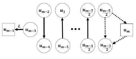
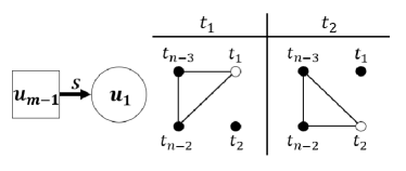
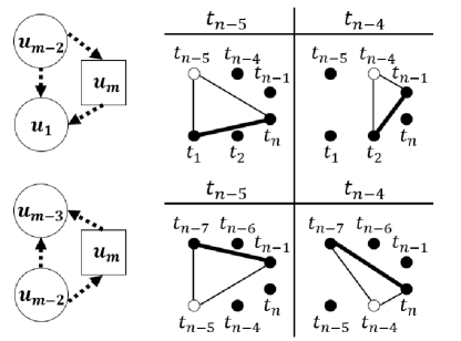
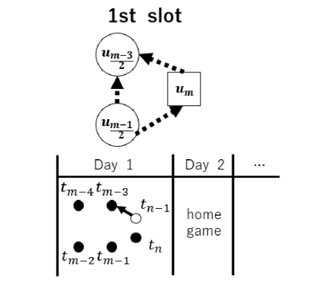
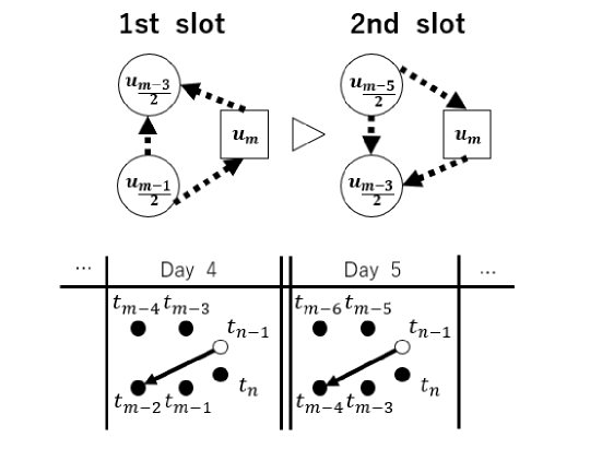
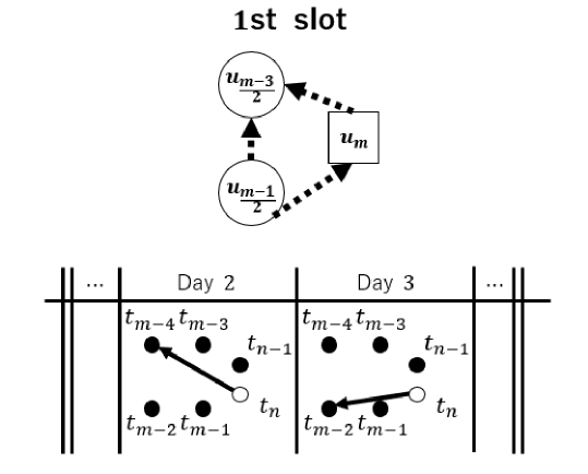
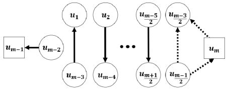
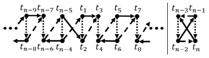
In the first slot, the super-teams are arranged as shown in Figure 1 if (mod 8). For the case (mod 8), the three dotted edges are reversed (the rightmost straight edge ( is also reversed). The two and three super-teams connected by the directed edges form a super-game. The super-game composed of three super-teams on the right is called a right super-game, and the other super-games of two super-teams are called normal super-games. The direction of the edge(s) in a super-game determines the games in the super-game, which will be explained below.
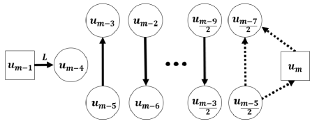
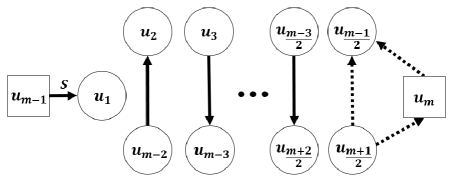
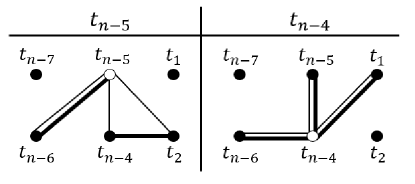
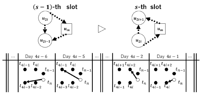
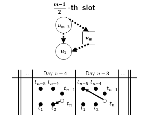
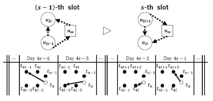
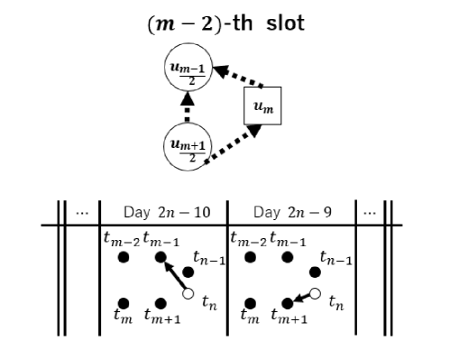
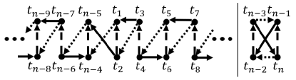
After the first slot, all super-teams except for and , i.e., the super-teams shown by circles in Figure 1, change the positions by moving one position in the clockwise direction, and all directed edges except for the leftmost edge incident to are reversed. Consequently, in the second slot, the super-teams are arranged as shown in Figure 8 in Appendix 5. The remaining slots are defined in the same manner. One exception is that the direction of the leftmost edge is reversed in each slot. The arrangement in the third slot is shown in Figure 9 in Appendix 5, and in the -th slot in Figure 10 in Appendix 5. From the second slot to the -th slot, the super-game including is called a left super-game , represented by in Figure 8 and Figure 9 in Appendix 5. Hence, in these slots, there are one left super-game, normal super-games and one right super-game. The left super-game in the -th slot is particularly called a special left super-game , represented by in Figure 10 in Appendix 5.
At the end of the -th slot, each team () has played two games against teams and has played no game against the other three teams. For , teams and in a super-team have played no game against each other, and against two of the four teams in the adjacent two super-teams. Teams , , and have played no game against the three of these four teams except for itself. Games against those three teams are played in the -th slot, which is in particular called the last slot, consisting of six days.
Next, we show how to set up the games in the super-games.
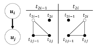
Normal super-games:
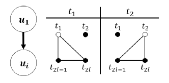
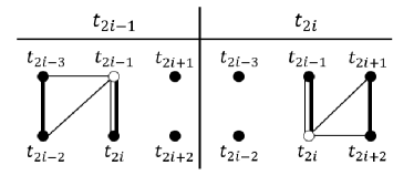
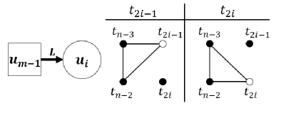
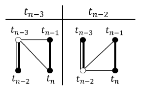
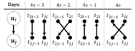
Each normal super-game is composed of eight games on four days. Let a normal super-game of super-teams and is held in the -th slot, where the direction of the edge is from to and . Recall that the super-team consists of two teams and , and of and . The eight games in this super-game will be played in days from to , as shown in Figure 2. In Figure 2, each directed edge represents a game held in the home venue of the team of the tail vertex.
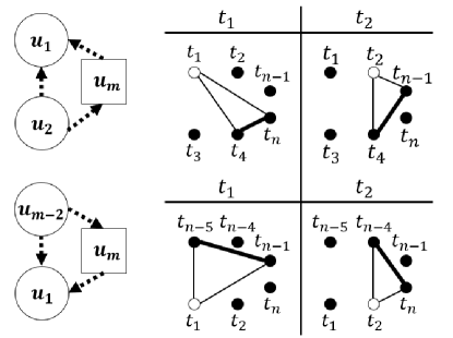
Left super-games:
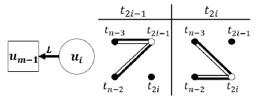
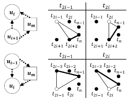
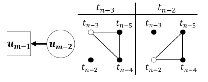
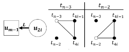
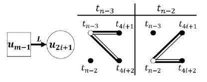
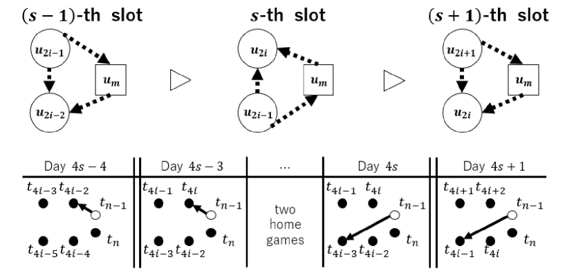
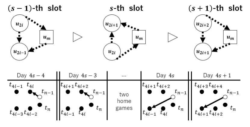
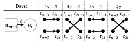
Each left super-game is composed of eight games on four days. Let a left super-game of super-teams and is held in the -th slot (, , ), and suppose that the direction of the edge is from to . Recall that the super-team consists of two normal teams and . The eight games in this super-game will be played in days from to , as shown in Figure 3. If directed edge between two super-teams is reversed, all directed edge between two teams are reversed.
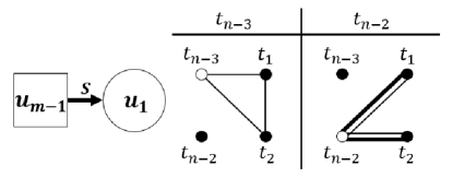
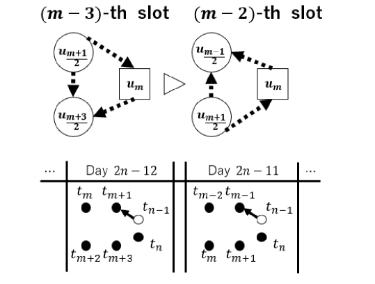
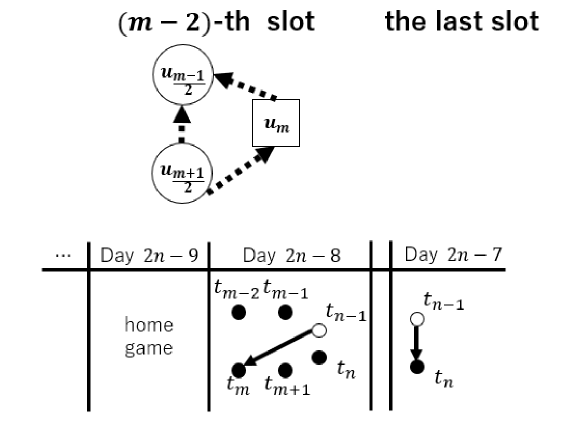
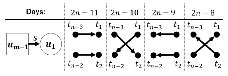
The special left super-game in the -th slot consists of super-teams and . The eight games in this super-game will be played in days from to , as shown in Figure 4. Special left super-game differs from other left super-games in that the edges incident to team on days and are reversed.
Right super-games:
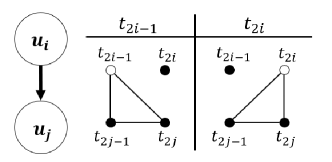
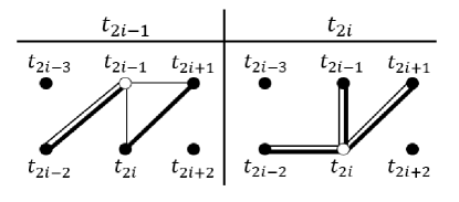
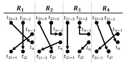
A right super-game consists of twelve games on four days, played by three super-teams (six teams). For concise notation, let . Let the super-game be held in the -th slot, and denote the three super-teams by , and ( (mod )). Suppose that the direction of the edges are from to , from to and from to .
The three games in each day are of eight types, , shown in Figure 5. For , the type is obtained from by reversing the edges. For , if there is a directed edge from to , the four days are arranged as , and otherwise . For , there is a directed edge from to , and the four days are arranged as . For , if there is a directed edge from to , the four days are arranged as , and otherwise .
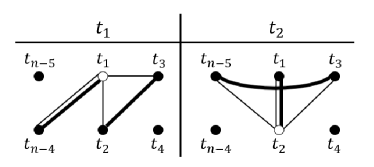
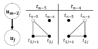
The last slot:
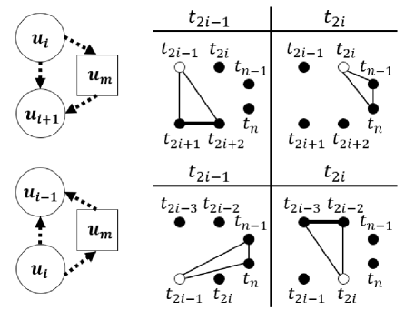
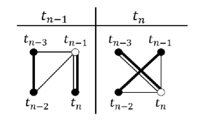
The first three days are shown in Figure 6, and the last three days in Figure 7. Figures 6 and 7 have directed edges of three types. A straight directed edge represents a game on the first day in Figure 6 and on the fourth day in Figure 7. A dotted directed edge represents a game on the second day in Figure 6 and on the fifth day in Figure 7. A broken directed edge represents a game on the third day in Figure 6 and on the sixth day in Figure 7.
3 Our Algorithm
In this section we present our algorithm. The algorithm is designed by combining the construction of the tournament by Zhao and Xiao [17] described in Section 2.2 and the numbering of the teams based on the idea of Imahori [7].
3.1 Numbering of the Teams
Recall that is a minimum weight perfect matching in and the two teams and must be connected by an edge in so that they form a super-team (). We determine four teams , and , forming two super-teams and , so that is the smallest and is the second smallest of . The other teams are numbered arbitrarily as long as is an edge in for each .
3.2 Analyzing the Approximation Ratio
Here we describe the analysis of the approximation ratio in the case of (mod 8). The case of (mod 8) can be analyzed in the same way.
Recall the lower bound (1), and define an extra traveling as a traveling of an edge that is not counted in defining (1). We estimate the distances of the extra travelings according to the following categorization of the super-teams into six classes.
Category : Super-team .
Teams and in super-team will play normal super-games, one special left super-game, two right super-games, and six games in the last slot. The travels of teams and are shown in Figures 11–14 in Appendix 5. In the normal super-games and the special left super-game, teams and have no extra traveling. The distance of the extra traveling of in the two right super-games is , and that of is . The distance of the extra traveling of in the six games in the last slot is , and that of is . These extra traveling distances are summarized in Table 1.
| Right super-games | (I-a) | (I-b) |
|---|---|---|
| Six games in the last slot | (I-c) | (I-d) |
Category : Super-teams .
Teams and in super-team will play normal super-games, one left super-game, two right super-games, and six games in the last slot. The travels of teams and are shown in Figure 15–18 in Appendix 5. The distances of the extra traveling are summarized in Table 2.
| Left | (II-a) | (II-b) |
|---|---|---|
| Right | (II-c) | (II-d) |
| Six games | (II-e) | (II-f) |
Category : Super-teams .
Teams and in super-team will play normal super-games, one left super-game, two right super-games, and six games in the last slot. The travels of teams and are shown in Figure 19–22 in Appendix 5. The distances of the extra traveling are summarized in Table 3.
| Right | (III-a) | (III-b) |
|---|---|---|
| Six games | (III-c) | (III-d) |
Category : Super-team .
Teams and in super-team will play normal super-games, two right super-games, and six games in the last slot. The travels of teams and are shown in Figure 23–25 in Appendix 5. The distances of the extra traveling are summarized in Table 4.
| Right | (IV-a) | (IV-b) |
|---|---|---|
| Six games | (IV-c) | (IV-d) |
Category : Super-team .
Teams and in super-team will play one normal super-game, left super-games, and six games in the last slot. The travels of teams and are shown in Figure 26–30 in Appendix 5. The distances of the extra traveling are summarized in Table 5.
| Left | (V-a) | (V-b) |
| Six games | (V-c) | (V-d) |
Category : Super-team .
Teams and in super-team will play right super-games, and six games in the last slot. The travels of teams and are shown in Figure 31–42 in Appendix 5. The distances of the extra traveling are summarized in Table 6.
| Right | (VI-a) | (VI-b) |
| Six games | (VI-c) | (VI-d) |
We have enumerated the distances of the extra travelings of all teams . We provide an upper bound of some of these distances by using triangle inequality, as shown Table 7.
| Distance | Upper bound | |
|---|---|---|
| (I-c) | ||
| (I-d) | ||
| (III-c) | ||
| (III-d) | ||
| (IV-c) | ||
| (IV-d) | ||
| (VI-a) | ||
| } | ||
| (VI-b) | ||
| (VI-c) | ||
It follows that all terms of these upper bounds and the distances of the extra travelings covered by the upper bounds are of the following three types:
-
(A)
;
-
(B)
; and
-
(C)
.
For each of these three types, we provide an upper bound of the sum of the distances in the following manner. First, we focus on Type (A). The distances and appear in (I-a), (I-b), (I-d), (II-a), (II-b), (III-a), (III-b), (IV-a), (IV-b), (IV-c), (IV-d), (V-a), (V-b), (V-c), (V-d), (VI-a), (VI-c), and (VI-d). Observe that each of and appears at most once, and hence the sum of the distances of Type (A) is at most
| (5) |
Second, we focus on the distances of Type (B). These appear in (I-c), (I-d), (III-c), (III-d), (IV-c), (IV-d), (VI-a), and (VI-b). Observe that each of appears at most five times, and hence the sum of the distances of Type (B) is at most
| (6) |
Last, we focus on the distances of Type (C). These appear in (I-c), (I-d), (II-c), (II-d), (II-e), (II-f), (III-c), (III-d), (IV-c), (IV-d), (VI-a), and (VI-b). Observe that each of appears at most six times, and hence the sum of the distances of Type (C) is at most
| (7) |
We have provided upper bounds on the extra traveling distances. Finally, we investigate the distances counted in the lower bound (1), because some of the edges in the perfect matching are not traveled by the two teams and in our tournament. In the first slots, each of and plays right super-games and the two opponents in one right super-game are in different super-teams. Hence, each of does not appear in the traveling of and . Accordingly, the distances of the edges counted in the lower bound (1) and used in our tournament is at most
| (8) |
Therefore, by summing (5), (6), (7), and (8), we obtain that the total traveling distance is at most
It follows from (3) and (4) that it is at most
Recall that is lower bound (1). We thus conclude that the approximation ratio of our algorithm is .
Theorem 1.
The approximation ratio of our algorithm is .
3.3 Analyzing the Time Complexity
Recall that is a complete graph with vertices. Let denote the maximum weight of an edge in , and the time complexity for finding a minimum weight perfect matching in . Currently,
We first compute a minimum weight perfect matching in . We second compute the sum of of the two teams in each edge of to determine and , which requires time. Thus, the computation time of dominates the other, and hence the computation time of our algorithm is , which is .
Theorem 2.
The time complexity of our algorithm is .
4 Conclusion
We have presented a deterministic -approximation algorithm for TTP-2, where is the number of the teams satisfying (mod 4). This algorithm runs in time. Compared with the deterministic -approximation algorithm by Zhao and Xiao [17], which runs in time, our algorithm has better complexity. Compared with the algorithm having the same complexity [7, 16], our algorithm has a better approximation ratio.
One direction of future work is to improve the approximation ratio. There is a gap between the total traveling distance in our algorithm and its upper bound obtained in Section 3.2. Possibly a further analysis of the upper bound results in a better approximation guarantee of our algorithm. Another direction is to investigate the time complexity of TTP-2. For , TTP- is shown to be NP-hard by Thielen and Westphal [11]. However, the complexity of TTP-2 is still not revealed, while a number of approximation algorithms are designed.
References
- [1] R. T. Campbell and D. Chen. A minimum distance basketball scheduling problem. Management Science in Sports, 4:15–26, 1976.
- [2] D. Chatterjee and B. K. Roy. An improved scheduling algorithm for traveling tournament problem with maximum trip length two. arXiv:2109.09065, 2021.
- [3] D. de Werra. Some models of graphs for scheduling sports competitions. Discrete Appl. Math., 21(1):47–65, 1988.
- [4] K. Easton, G. Nemhauser, and M. Trick. The traveling tournament problem description and benchmarks. In 7th CP, pages 580–584. Springer, 2001.
- [5] H. N. Gabow. Implementation of Algorithms for Maximum Matching on Nonbipartite Graphs. PhD thesis, Department of Computer Science, Stanford University, Stanford, California, 1973.
- [6] H. N. Gabow and R. E. Tarjan. Faster scaling algorithms for general graph matching problems. J. ACM, 38(4):815–853, 1991.
- [7] S. Imahori. A 1+ approximation algorithm for (2). arXiv:2108.08444, 2021.
- [8] S. Imahori, T. Matsui, and R. Miyashiro. A 2.75-approximation algorithm for the unconstrained traveling tournament problem. Ann. Oper. Res., 218(1):237–247, 2014.
- [9] E. L. Lawler. Combinatorial Optimization: Networks and Matroids. Holt, Rinehart and Winston, New York, 1976.
- [10] R. Miyashiro, T. Matsui, and S. Imahori. An approximation algorithm for the traveling tournament problem. Ann. Oper. Res., 194:317–324, 2012.
- [11] C. Thielen and S. Westphal. Complexity of the traveling tournament problem. Theor. Comput. Sci., 412(4-5):345–351, 2011.
- [12] C. Thielen and S. Westphal. Approximation algorithms for (2). Math. Methods Oper. Res., 76:1–20, 2012.
- [13] M. Xiao and S. Kou. An improved approximation algorithm for the traveling tournament problem with maximum trip length two. In 41st MFCS, LIPIcs, volume 58, pages 89:1–89:14, 2016.
- [14] D. Yamaguchi, S. Imahori, R. Miyashiro, and T. Matsui. An improved approximation algorithm for the traveling tournament problem. Algorithmica, 61(4):1077–1091, 2011.
- [15] J. Zhao and M. Xiao. A further improvement on approximating -2. In 27th COCOON, LNCS, volume 13025, pages 137–149. Springer, 2021.
- [16] J. Zhao and M. Xiao. The traveling tournament problem with maximum tour length two: A practical algorithm with an improved approximation bound. In 30th IJCAI, pages 4206–4212, 2021.
- [17] J. Zhao and M. Xiao. Practical algorithms with guaranteed approximation ratio for with maximum tour length two. arXiv:2212.12240, 2022.
- [18] J. Zhao and M. Xiao. A -approximation algorithm for the traveling tournament problem. arXiv:2309.01902, 2023.
- [19] J. Zhao, M. Xiao, and C. Xu. Improved approximation algorithms for the traveling tournament problem. In 47th MFCS, LIPIcs, volume 241, pages 83:1–83:15, 2022.
5 Supplementary Figures
We show Figures 8–10 and Figures 11–42, which are omitted in Section 2.2 and Section 3.2, respectively.