Evaluation of metrology using self-consistent approach in the MCTDH theory

Self-consistent many-body metrology

Abstract

We investigate performing classical and quantum metrology and parameter estimation by using interacting trapped bosons, which we theoretically treat by a self-consistent many-body approach of the multiconfigurational Hartree type. Focusing on a tilted double-well geometry, we compare a self-consistently determined and monitored two-mode truncation, with dynamically changing orbitals, to the conventional two-mode approach of fixed orbitals, where only Fock space coefficients evolve in time. We demonstrate that, as a consequence, various metrological quantities associated to a concrete measurement such as the classical Fisher information and the maximum likelihood estimator are deeply affected by the orbitals’ change during the quantum evolution. Self-consistency of the quantum many-body dynamics of interacting trapped ultracold gases thus fundamentally affects the attainable parameter estimation accuracy of a given metrological protocol.

Within the currently emerging quantum era, quantum metrology [1, 2, 3, 4, 5, 6, 7, 8] has proven itself to be a powerful tool for the accurate estimation of even very small physical parameters, such as gravitational wave amplitudes [9], or to limit the attainable measurement accuracy of fundamental constants like the speed of light [10]. As a result, quantum metrology promises to revolutionize the existing technologies of measurement.

While quantum metrology has frequently been employed in the quantum optical context [11, 12, 13, 14], more recently the corresponding experiments and theory are also exploring coherent matter waves cf., e.g., Refs. [15, 16, 17, 18, 19, 20, 21, 22, 23, 24, 25, 26, 27, 28, 29, 30, 31]. Photons freely propagating in the quantum vacuum are to a very good approximation noninteracting particles and are well described by plane waves of definite momentum. Matter waves forming Bose-Einstein condensates at very low temperatures are, however, interacting by the scattering of their elementary atomic or molecular constituents, and are spatially confined (trapped) by arbitrary scalar potentials. In what follows, we show that the full self-consistency of the quantum many-body evolution of such a system needs in general to be taken into account, to yield reliable parameter estimation. We demonstrate that the interplay of Fock space amplitudes and time-dependent field operator modes ($\coloneqq$ orbitals), the hallmark of self-consistent many-body evolution, is crucial. This interplay is not obtained when fixing the orbitals’ shape, thereby significantly restricting the associated Hilbert space.

We take as an archetypical model system and for concreteness a tilted double well, where the parameter to be estimated is the linear slope $p_{4}$ which could, e.g., represent exposing the gas to constant gravitational acceleration (see Fig. 1). To facilitate comparison with conventional interferometry, we stay for the whole time evolution in a (continuously monitored) two-mode approximation (TMA), corresponding to two interferometric arms. We consider a simple (Mach-Zehnder type) experiment which counts at the instant of measurement the number of particles on the left and right. It is demonstrated that while a non-self-consistent evolution yields a null result for $p_{4}$ [zero classical Fisher information (CFI)], a self-consistent quantum many-body evolution gives finite CFI, enabling $p_{4}$ estimation.

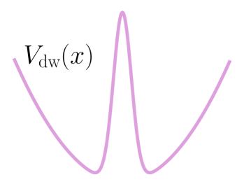
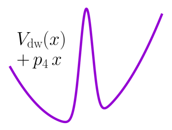
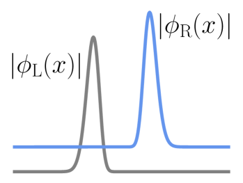
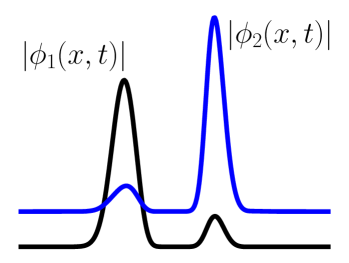
Figure 1: Top: Trap potential. Left: $t<0$, symmetric double well. Right: At $t=0$, the tilt is switched on. Bottom: Initially localized orbitals in the large-barrier double-well self-consistently evolve in time after tilting, and become delocalized, whereas without self-consistency they remain localized. The orbitals are vertically offset for clarity.

To determine the self-consistent evolution during the metrological protocol, we employ the multiconfigurational time-dependent Hartree (MCTDH) method [32, 33, 34, 35]. The general $N$-body state is described by the ansatz

$$|\Psi(t)\rangle=\sum\limits_{\vec{n}}C_{\vec{n}}(t)|\vec{n}(t)\rangle\,,\vspace*{-0.25em}$$ (1)

where $\sum_{\vec{n}}|C_{\vec{n}}|^{2}=1$ for state normalization and $\vec{n}$ denotes the set of occupation numbers $\{n_{i}\,|\,i=1,2,\cdots,M\}$ in each mode (orbital), with $\sum_{i=1}^{M}n_{i}=N$. The time-dependent Fock basis state $|\vec{n}(t)\rangle$ indicates that the orbitals change in time as a result of finite $M$ (see, Fig. 1). Their dynamics follows the system of nonlinear coupled integrodifferential Eqs. (S1) in the supplement [36]. Numerical solution enables the determination of Fock space coefficients $C_{\vec{n}}$ and orbitals at any time. Further details on the MCTDH-X implementation of MCTDH, used to solve Eqs. (S1), can be found in Ref. [35].

The quantum metrological approach to parameter estimation, see for example Refs. [37, 38, 39, 40, 41], proceeds essentially as follows. An initial state $|\psi\rangle$ experiences a dynamical evolution, e.g., $e^{-i\hat{H}_{X}t}$, during the time $t$ and the final state $|\psi_{X}\rangle$ contains the information of the parameter $X$. One chooses an appropriate measurement on $|\psi_{X}\rangle$ to estimate $X$. Previous studies on quantum metrology with ultracold atoms [15, 16, 17, 18, 19, 20, 21, 22, 23, 24, 25, 26, 27, 28, 29, 30, 31] have focused on the coefficients $C_{\vec{n}}(X;t)$ in Eq. (1), and have calculated the quantum Fisher information ${\mathfrak{F}}_{X}$ (QFI) from $C_{\vec{n}}(X;t)$ only. However, since the orbitals also evolve by Eqs. (S1) and the time evolution relies on $X$, the $|\vec{n}(X;t)\rangle$ must be considered in the calculation of the QFI as well as the CFI. To evaluate the sensitivity of a quantum mechanical state to a parameter change thus requires full exploitation of the information encoded in the state. Here, we make full use of the parameter dependence of the state, reflected in both coefficients and orbitals. We establish thereby numerically exact parameter estimation for trapped interacting quantum gases.

A single component bosonic gas with contact interactions, trapped in a quasi-one-dimensional (quasi-1D) double-well potential, is described by the Hamiltonian

$$\hat{H}=\sum_{j=1}^{N}\Big{\{}-\frac{1}{2}\frac{\partial^{2}}{\partial x_{j}^{2}}+V(x_{j})\Big{\}}+g\sum^{N}_{j<k}\delta(x_{j}-x_{k}),$$ (2)

where $V$ is the trap potential. We render $\hat{H}$ in a dimensionless form, fixing a unit length $L$ . The quasi-1D interaction coupling $g$ is controllable by either Feshbach or geometric scattering resonances and by transverse trapping [43]. Exact solutions of the Schrödinger equation associated to Eq. (2) exist for homogeneous gases under periodic boundary conditions or in a box trap; their metrological properties were explored in [44].

We assume a trap potential of the form $V(x)=V_{\rm dw}(x)+p_{4}x=\frac{1}{2}p_{1}x^{2}+p_{2}\exp[-x^{2}/(2\,p_{3}^{2})]+p_{4}\,x$, where $p_{4}=0$ initially, cf. Fig. 1. The remaining parameters, $p_{1}=0.5$, $p_{2}=50$, and $p_{3}=1$, are fixed throughout the dynamical evolution. The two lowest energy single-particle states are symmetric and antisymmetric with respect to the origin, respectively, and addition and subtraction of them result in two well-localized orbitals: left $\phi_{\rm L}(x)$ and right $\phi_{\rm R}(x)$, see Fig. 1. These orbitals, as approximate ground states of each well, are the basic one-particle states that furnish the two modes [45].

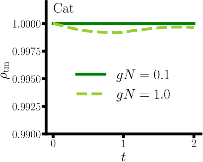
Figure 2: Monitoring the two-mode truncation after $p_{4}$ is turned on, by verifying whether $\rho_{\rm tm}=(\rho_{1}+\rho_{2})/N\lesssim 1$ (we put $N=10$), with $gN$ values as indicated. Cat state is on the left and spin coherent state on the right.

The estimation process of $p_{4}$ proceeds as follows. An initial state represented in the form of Eq. (1) is supposed to be created. With $\phi_{\rm L}(x)$ and $\phi_{\rm R}(x)$, we employ two coefficient distributions: A NOON (cat) state, which has $|\psi_{0}\rangle=(|N,0\rangle+|0,N\rangle)/\sqrt{2}$, and a spin coherent state $|\psi_{0}\rangle=\sum_{k=0}^{N}\sqrt{\frac{N!}{k!\,(N-k)!}}\cos^{N-k}(\frac{\pi}{4})\sin^{k}(\frac{\pi}{4})|N-k,k\rangle$. Then a small $p_{4}$ is switched on, tilting trap potential tilted and making it asymmetric. The state then evolves according to Eqs. (S1); finally, the number of particles in each well is measured and $p_{4}$ is estimated from the set of measurement outcomes.

As the relative interaction strength $gN$, a typical ratio of interaction over single-particle energies, increases, more modes than two ($M=2$) are required to correctly reproduce the many-body dynamics [46]. In order to adequately compare the self-consistent (SC) results to those of the conventional SU(2) two-mode interferometry (TMI), which operates with the Fock space coefficients only, we maintain the validity of the TMA throughout the time evolution. This can be assessed by evaluating $\rho_{\rm tm}\coloneqq(\rho_{1}+\rho_{2})/N$, cf. Fig. 2, where $\rho_{j}$ is the $j$th largest eigenvalue of the reduced one-body density matrix, $\rho^{(1)}(x,x^{\prime};t)$ [Eq. (S2)]. After diagonalization, $\rho^{(1)}(x,x^{\prime})=\sum_{j}\rho_{j}(t)\,\phi_{j}^{({\rm no})\ast}(x^{\prime},t)\,\phi_{j}^{({\rm no})}(x,t)$, with the natural orbitals $\{\phi_{j}^{({\rm no})}(x,t)|\,j=1,2,\cdots\}$. When a single $\rho_{1}=O(N)$ (in the formal limit $N\rightarrow\infty$), a Bose-Einstein condensate is obtained. For several $\rho_{j}$ of $O(N)$, we have a fragmented condensate [47]. The validity of the TMA (two-fold fragmented condensate) depends on whether $\rho_{1}\simeq\rho_{2}\simeq N/2$ and $\rho_{\rm tm}\simeq O(1)$ hold.

We define an initial state using four orbitals ($M=4$), which are including $\phi_{\rm L}(x)$ and $\phi_{\rm R}(x)$, and then monitor the natural occupations $\rho_{j}$ while the state evolves in time self-consistently under nonzero $p_{4}$, for both cat and spin coherent states. Fig. 2 shows the monitoring of $\rho_{\rm tm}$, where we observe it is close to unity. Also, both $\rho_{1}$ and $\rho_{2}$ are macroscopically occupied during the evolution, with negligible occupations $\rho_{3}$ and $\rho_{4}$. This fact however also depends on the parameter regime used. When $gN=0.1$, two modes are sufficient, but when $gN=1$, $\rho_{\rm tm}$ discernibly dips below unity. Increasing $p_{4}$ further, the TMA fails. An appropriate regime of parameters where $\rho_{\rm tm}\simeq 1$ is obtained when we fix $gN=0.1$ and $p_{4}=0.1$. Also, even though the natural orbitals are used in the discussion above, we can apply the two-mode criterion to the left/right orbitals or their time-evolved forms, i.e., $\phi_{1}(x,t)$ and $\phi_{2}(x,t)$, since there always exists a unitary transformation such that $\phi_{j}(x,t)=\sum_{jk}U_{jk}\,\phi_{k}^{({\rm no})}(x,t)$.

When the second-quantized form of Eq. (2) is two-mode expanded with $\hat{\Psi}(x)=\hat{b}_{\rm L}\,\phi_{\rm L}(x)+\hat{b}_{\rm R}\,\phi_{\rm R}(x)$, a two-site single-band Bose-Hubbard model Hamiltonian is obtained. In terms of the usual SU(2) Pauli matrices $\hat{J}_{x}=\frac{1}{2}(\hat{b}_{\rm L}\hat{b}_{\rm R}+\hat{b}^{\dagger}_{\rm R}\hat{b}_{\rm L})$ and $\hat{J}_{z}=\frac{1}{2}(\hat{b}_{\rm L}\hat{b}_{\rm L}-\hat{b}^{\dagger}_{\rm R}\hat{b}_{\rm R})$,

$$\hat{H}=-\tau\hat{J}_{x}+\epsilon\,\hat{J}_{z}+U\hat{J}_{z}^{2}\,,$$ (3)

where $\tau$ is tunneling amplitude, $\epsilon$ indicates an energy offset between wells, and $U\propto g$ is the interaction coupling, all of which depend on integrals involving the two orbitals. The implementation of quantum metrological protocols using the above Hamiltonian was carried out, e.g., in Refs. [20, 25, 41]: An initial state $|\psi_{0}\rangle$, as defined by the distribution of coefficients $C_{\vec{n}}$, evolves as $\exp(-i\hat{H}t)|\psi_{0}\rangle$, and the parameter of interest, e.g., $\epsilon$, is estimated from the population imbalance between the two modes [20, 25]. In our setup, the strong barrier renders the initial $\tau$ exponentially small compared to $\epsilon$ and $U$, and $\epsilon\neq 0$, as the symmetry of $V(x)$ is broken by $p_{4}$. Hence the TMI time evolution operator is, to very good accuracy, $\exp(-i(\epsilon\hat{J}_{z}+U\hat{J}_{z}^{2})t)$, and the QFI can be analytically calculated by $\mathfrak{F}_{\epsilon}=4\,\langle\psi_{0}|(\Delta\hat{J}_{z})^{2}|\psi_{0}\rangle$. When the cat state is used, $\mathfrak{F}_{\epsilon}=N^{2}\,t^{2}$, which is denoted as the Heisenberg limit. For the spin coherent state, $\mathfrak{F}_{\epsilon}=N\sin^{2}(\theta)\,t^{2}$, which represents the shot-noise limit (the so-called standard quantum limit). Any nonzero $\tau$ deteriorates the $N$-scaling of $\mathfrak{F}_{\epsilon}$, which can be confirmed by numerically calculating the QFI [20]. Note that here only the change of Fock space coefficients has been considered, while the orbital basis is fixed in TMI. Because of the latter fact, the still exponentially small $\tau$ and $U$ are kept constant during the evolution, and $\epsilon$ is abruptly switched on at $t=0$. In our setting, $\epsilon\in(-0.7,-0.6)$, and $U\in(0.002,0.03)$, with concrete values determined by $gN$ and $N$, on which in turn the initial orbitals $\phi_{\rm L}(x)$ and $\phi_{\rm R}(x)$ depend. Recall that our target parameter is $p_{4}$, not $\epsilon$, thus by using the chain rule, $\mathfrak{F}_{p_{4}}=\mathfrak{F}_{\epsilon}\times(h_{1}-h_{2})^{2}$, where the single-particle energies $h_{i}\coloneqq\int dx\,\phi_{i}^{\ast}(x)\left[-\frac{1}{2}\frac{\partial^{2}}{\partial x^{2}}+V(x)\right]\phi_{i}(x)$.

First, we compare the QFIs of the SC approach and the conventional TMI. The QFI with respect to a given parameter $X$ inscribed onto a pure state $|\psi_{X}\rangle$, is $\mathfrak{F}_{X}=4\big{(}\langle\partial_{X}\psi_{X}|\partial_{X}\psi_{X}\rangle-|\langle\psi_{X}|\partial_{X}\psi_{X}\rangle|^{2}\big{)}$, and insertion of Eq. (1) into $|\psi_{X}\rangle$ gives Eq. (S4), which facilitates calculation of the QFI using the ingredients of MCTDH theory from the expansion in Eq. (1). The first row in Fig. 3 shows the QFI versus time $t$ and particle number $N$, respectively. For each initial state, the SC method reproduces very well the QFI predicted by TMI. The influence of self-consistency thus plays a subdominant role for $\mathfrak{F}_{X}$, as the latter completely depends on the final state itself, and the self-consistency (changing orbitals) essentially represents fitting that state more exactly. When the bosons weakly interact ($gN=0.1$) and the disturbance to the system is small ($p_{4}=0.1$), conventional TMI therefore approximates well the QFI. We have verified in this regard that terms containing Fock space coefficients only and those involving orbitals, in the general relation for ${\mathfrak{F}}_{X}$ [Eq. (S4)], tend to compensate each other.

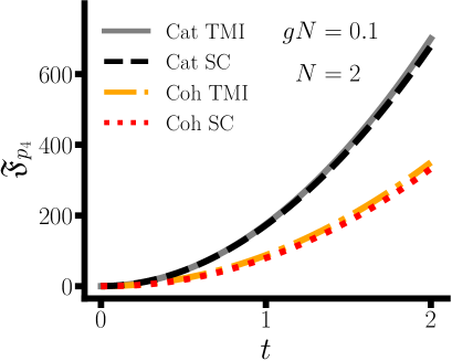
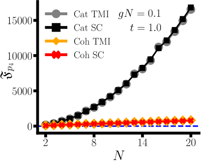
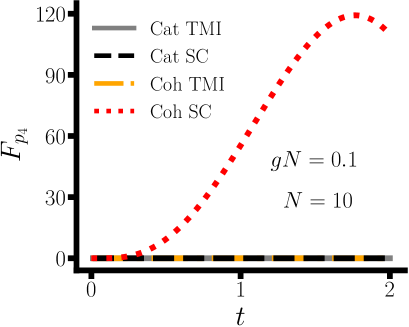
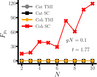
Figure 3: First and second row display quantum ($\mathfrak{F}$) and classical (F) Fisher information, respectively, plotted versus time $t$ (left) and particle number $N$ (right), for cat and coherent (coh) states, respectively. At the maximum on the lower left plot, which is at $t=1.77$, the tunneling amplitude in the SC evolution has increased to $\tau\simeq 0.09$ (for $N=10$).

We now turn to the CFI [48, 49], associated to a concrete measurement, for which, as we show, the impact of self-consistency becomes manifest. Since counting the number of bosons in each well constitutes our measurement, the corresponding CFI is defined as

$$F_{p_{4}}=\sum_{\vec{\mathbf{n}}}P(\vec{\mathbf{n}}|p_{4})\Big{(}\frac{\partial\log P(\vec{\mathbf{n}}|p_{4}))}{\partial\,p_{4}}\Big{)}^{2}\,,$$ (4)

where $P(\vec{\mathbf{n}}|p_{4})$ is the probability distribution (likelihood) of the measurement outcomes $\vec{\mathbf{n}}=(n_{\rm L},n_{\rm R})$, given $p_{4}$, and $n_{\rm L}$ and $n_{\rm R}$ are the numbers of particles that reside in the left and the right well, respectively. An appropriate $P(\vec{\mathbf{n}}|p_{4})$ has to be constructed to calculate the CFI and the conventional TMI approach considers that $P(\vec{\mathbf{n}}|p_{4})\coloneqq|\langle\vec{n}(t)|\Psi(t)\rangle|^{2}$. Then, the CFI always exactly vanishes, irrespective of the initial state, as the Hamiltonian contains only $\hat{J}_{z}$ and $\hat{J}_{z}^{2}$. The corresponding TMI time evolution therefore just changes the phases of the coefficients: $C_{k}(t)=\exp(-i\epsilon\frac{N-2k}{2}t)\,\exp(-iU(\frac{N-2k}{2})^{2}t)\,C_{k}(0)$, where the state $|\psi(t)\rangle=\sum_{k=0}^{N}C_{k}(t)|N-k,k\rangle=\exp(-i(\epsilon\hat{J}_{z}+U\hat{J}_{z}^{2})t)|\psi(0)\rangle$ and $\hat{J}_{z}|N-k,k\rangle=\frac{N-2k}{2}|N-k,k\rangle$. Then $P(\vec{\mathbf{n}}=(N-k,k)|p_{4})=|C_{k}(t)|^{2}=|C_{k}(0)|^{2}$, independent of $p_{4}$, yielding vanishing CFI in the TMI approach [36].

On the other hand, when the orbitals evolve together with the Fock space coefficients in the SC framework, the initial interpretation of the orbitals cannot be maintained throughout the time evolution. Initially well-localized orbitals, i.e., $\phi_{\rm L}(x)=\phi_{1}(x,0)$ and $\phi_{\rm R}(x)=\phi_{2}(x,0)$, correspond to particles being found in the left and right well, respectively. However, the orbitals change with time during the many-body evolution, thus the orbitals at a later time, i.e., $\phi_{1}(x,t)$ and $\phi_{2}(x,t)$, do not necessarily imply left or right localization at the time of measurement. Therefore, simply computing $P(\vec{\mathbf{n}}|p_{4})=|\langle\vec{n}(t)|\Psi(t)\rangle|^{2}$, as in the TMI approach, is not applicable. In the bosonic field operator $\hat{\Psi}(x)=\sum_{j}\hat{b}_{j}(t)\,\phi_{j}(x,t)$, it is clear that the bosonic annihilation operator $\hat{b}_{j}(t)$ corresponds to the time-evolving orbital $\phi_{j}(x,t)$, which delocalizes with increasing $t$, see Fig. 1. Thus the Fock state in Eq. (1)

$$|\vec{n}(t)\rangle=\frac{\big{(}\hat{b}_{1}^{\dagger}(t)\big{)}^{n_{1}}\big{(}\hat{b}_{2}^{\dagger}(t)\big{)}^{n_{2}}\cdots\big{(}\hat{b}_{M}^{\dagger}(t)\big{)}^{n_{M}}}{\sqrt{n_{1}!n_{2}!\cdots n_{M}!}}|0\rangle$$ (5)

cannot by itself appropriately project the quantum state into any of $|\vec{\mathbf{n}}\rangle$ and $\langle\vec{n}(t)|\Psi(t)\rangle$ cannot be interpreted as the probability amplitude for each measurement outcome as in TMI. In other words, $|\vec{n}(t)\rangle$ and $|\vec{\mathbf{n}}\rangle$ are different in the SC approach. Hence it is necessary to re-establish a connection between time-evolving orbitals and $|\vec{\mathbf{n}}\rangle$ that corresponds to a measurement outcome, resulting in the proper distribution $P(\vec{\mathbf{n}}|p_{4})=|\langle\vec{\mathbf{n}}|\Psi(t)\rangle|^{2}\neq|\langle\vec{n}(t)|\Psi(t)\rangle|^{2}$.

In the SC time evolution after the trap potential is tilted, $\phi_{1}(x,t)$ and $\phi_{2}(x,t)$ remain well-localized in the case of a cat state. That is, $\phi_{1}(x,t)$ ($\phi_{2}(x,t)$) begins from $\phi_{1}(x,0)=\phi_{\rm L}(x)$ [$\phi_{2}(x,0)=\phi_{\rm R}(x)$] and their absolute value remains nearly identical except slightly wider (narrower) width and shorter (taller) height, respectively. For the spin coherent state, however, $\phi_{1}(x,t)$ and $\phi_{2}(x,t)$ spread into opposite wells while they evolve under nonzero $p_{4}$; see Fig. 1. Then even when a particle resides in $\phi_{1}(x,t)$ or $\phi_{2}(x,t)$, to assign it to the left or right well is ambiguous. One can however still define mathematically “left” or “right” by integrating the orbitals from $-\infty$ to the center point $x=0$ of $V(x)$ and from the center point of $V(x)$ to $\infty$, respectively: $P_{\text{Left}}=\int_{-\infty}^{0}\!\!|\phi_{j}(x,t)|^{2}\,dx$ and $P_{\text{Right}}=\int_{0}^{\infty}\!\!|\phi_{j}(x,t)|^{2}\,dx$. One can then construct $P(\vec{\mathbf{n}}|p_{4})$ by computing the permanent of a special matrix composed from $P_{\text{Left}}$ and $P_{\text{Right}}$. The computable $N$ range is limited, though, due to rapidly increasing algorithmic complexity [36].

The second row in Fig. 3 shows the CFI versus $t$ and $N$. The conventional approach with fixed orbitals results in vanishing CFI, as expected. Also, even though the SC approach is used, the cat state shows almost vanishing CFI, which is attributed to the fact that the orbitals stay localized in each well during the whole evolution time and the probabilities, i.e., $P_{\text{Left}}$ and $P_{\text{Right}}$, remain nearly constant (for small $p_{4}$). Thus under the given measurement the change of $P(\vec{\mathbf{n}}|p_{4})$ with respect to $p_{4}$ is negligible. However, the spin coherent state displays a significant change in orbitals and increasing CFI during the early stage. Bottom right in Fig. 3 shows the $N$-scaling of the CFI, and here the SC approach with spin coherent state shows an almost linearly increasing CFI. The complex fluctuation pattern appears because of the short time $t=1.77$ after a nonzero $p_{4}$ is suddenly applied, and for increasing $t$ these fluctuations smoothen out. Thus a SC approach may yield drastically different metrological predictions from a TMI based method.

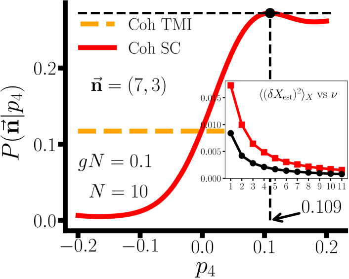
Figure 4: Shown is a single implementation of the MLE for an estimate of $p_{4}$ using the spin coherent state. Red solid line is for the SC approach and orange dashed line (a constant $\forall\,p_{4}$) for the TMI. In the inset, red squares represent the mean-square deviation and black rounds the Cramér-Rao lower bound from Eq. (6).

Fig. 4 shows our primary result: The implementation of parameter estimation at the final stage of the metrological protocol. The maximum likelihood estimator (MLE) [6, 50] is used as a concrete example here, because it asymptotically saturates the Cramér-Rao bound for an infinite number of measurements ($\nu\rightarrow\infty$) [36],

$$\langle(\delta X_{\text{est}})^{2}\rangle_{X}\geq\frac{1}{\nu F_{X}}\,.$$ (6)

Here, the parameter $X$ is our $p_{4}$, $X_{\text{est}}$ is an estimator of $X$, and $\delta X_{\text{est}}:=X_{\text{est}}/\big{|}\partial\langle X_{\text{est}}\rangle_{X}/\partial X\big{|}-X$, where the average $\langle\cdots\rangle_{X}$ is taken with respect to $P(\vec{\mathbf{n}}|p_{4})$.

In Fig. 4, the likelihood function $P(\vec{\mathbf{n}}|p_{4})$ is displayed supposing, for concreteness, that the measurement outcome is $\vec{\mathbf{n}}=(7,3)$, where $n_{\rm L}$ and $n_{\rm R}$ denote the number of particles found in left and right well, respectively. The red solid line shows the maximum of $P(\vec{\mathbf{n}}|p_{4})$ at $p_{4}\simeq 0.109$, thus the estimate of $p_{4}$ given $\vec{\mathbf{n}}=(7,3)$ is $X_{\text{est}}\simeq 0.109$. Similarly, every single outcome, $11$ in total, is connected to a corresponding estimate of $p_{4}$. The orange dashed line obtained by the conventional TMI approach with a spin coherent state stays flat, which means that the information given by the measurement outcome $\vec{\mathbf{n}}=(7,3)$ is zero, so one cannot extract an estimate of $p_{4}$, in accordance with $F_{p_{4}}=0$.

When $\langle X_{\text{est}}\rangle_{X}=X$ holds, an estimator is by definition unbiased. The present MLE is not unbiased except infinitesimally close to $p_{4}=0$ and the larger $p_{4}$, the more bias its estimation acquires. For instance, in Fig. 4, the true value of $p_{4}$ is $0.1$ and the bias of the MLE is on the level of 10 %, $\langle X_{\text{est}}\rangle_{X=0.1}\simeq 0.11$. Also, $\partial\langle X_{\text{est}}\rangle_{X}/\partial X|_{X=0.1}\simeq 0.6$, which then provides the mean-square deviation $\langle(\delta X_{\text{est}})^{2}\rangle_{X=0.1}$. The inset in Fig. 4 verifies that, asymptotically, $\langle(\delta X_{\text{est}})^{2}\rangle_{X=0.1}$ approaches the Cramér-Rao lower bound for large $\nu$.

In conclusion, we have found using a self-consistent many-body approach that the metrological outcome of a given measurement utilizing interacting confined bosons needs to conform to the final self-consistently computed many-body state. On one hand, the QFI completely depends on the parameter dependence of the final state itself, and is relatively unaffected by self-consistency (in the weakly interacting regime). On the other hand, even in the latter regime, the CFI for a parameter estimation experiment is strongly affected by self-consistency due to its sensitive dependence on the orbitals’ time evolution. As a particularly notable example, we have shown that fitting the outcome of a number-statistics experiment in a double well to conventional TMI gives a null result for estimating the slope parameter $p_{4}$. The SC approach we employ, however, enables $p_{4}$ estimation. We infer that metrology with ultracold quantum gases in general requires the self-consistency of dynamical evolution to correctly predict the estimation precision that can be accomplished in a given metrological protocol.

This work has been supported by the National Research Foundation of Korea under Grants No. 2017R1A2A2A05001422 and No. 2020R1A2C2008103.

I Supplemental Material

I.1 Multiconfigurational time-dependent Hartree theory

Given a set of coefficients and a set of orbitals for an initial state, the time evolution in the MCTDH framework proceeds according to the following system of equations:

$$i\,\frac{\partial\,\mathbf{C}(t)}{\partial\,t} = \mathbf{H}(t)\,\mathbf{C}(t)\,,$$

$$i\,\partial_{t}|\phi_{j}\rangle = \hat{P}\Big{[}\hat{h}|\phi_{j}\rangle+\sum_{k,s,q,l}[\rho^{-1}]_{jk}\rho_{ksql}\hat{W}_{sl}|\phi_{q}\rangle\Big{]},$$ (S1)

which is derived by applying the time-dependent variational principle to the interacting $N$-body Hamiltonian $\hat{H}=\sum_{j=1}^{N}\hat{h}(x_{j})+\sum_{j<k}\hat{W}(x_{j}-x_{k})$[33]. Here, $\mathbf{C}(t)$ is a column vector that consists of all possible expansion coefficients $C_{\vec{n}}(t)$ and $\mathbf{H}(t)$ corresponds to the time-dependent Hamiltonian matrix in the basis $\{|\vec{n}(t)\rangle\}$. Also, $\hat{h}$ is a single-particle Hamiltonian, $\hat{W}_{sl}=\int dx^{\prime}\,\phi_{s}^{\ast}(x^{\prime})\,\hat{W}(x-x^{\prime})\,\phi_{l}(x^{\prime})$, and $\hat{P}=1-\sum_{j=1}^{M}|\phi_{j}\rangle\langle\phi_{j}|$ is an projection operator to the subspace that is orthogonal to the one spanned by orbitals. The $[\rho^{-1}]_{jk}$ is a matrix element of the inverse of reduced one-body density matrix:

$$\rho(x,x^{\prime};t) = \langle\Psi(t)|\hat{\Psi}^{\dagger}(x^{\prime})\hat{\Psi}(x)|\Psi(t)\rangle$$ (S2)

$$= \sum_{k,q}\phi_{k}^{\ast}(x^{\prime},t)\phi_{q}(x,t)\langle\Psi(t)|\hat{b}_{k}^{\dagger}(t)\hat{b}_{q}(t)|\Psi(t)\rangle$$

$$= \sum_{k,q}\phi_{k}^{\ast}(x^{\prime},t)\phi_{q}(x,t)\rho_{kq}(t)\,,$$

where the $\rho_{kq}$ is, for the cases of $k=q$ and $k\neq q$,

$$\rho_{kk}=\sum_{\vec{n}}|C_{\vec{n}}(t)|^{2}n_{k},\quad\rho_{kq}=\sum_{\vec{n}}C_{\vec{n}}^{\ast}(t)C_{\vec{n}_{k}^{q}}(t)\sqrt{n_{k}(n_{q}+1)}\,.$$

Similarly, $\rho_{ksql}$ is a matrix element of the reduced two-body matrix

$$\rho(x_{1},x_{2},x^{\prime}_{1},x^{\prime}_{2};t) = \langle\Psi(t)|\hat{\Psi}^{\dagger}(x^{\prime}_{1})\hat{\Psi}^{\dagger}(x^{\prime}_{2})\hat{\Psi}(x_{1})\hat{\Psi}(x_{2})|\Psi(t)\rangle$$ (S3)

$$= \sum_{k,s,q,l}\phi_{k}^{\ast}(x^{\prime}_{1},t)\phi_{s}^{\ast}(x^{\prime}_{2},t)\phi_{q}(x_{1},t)\phi_{l}(x_{2},t)\rho_{ksql}(t)\,,$$

where

$$\rho_{kkkk} = \sum_{\vec{n}}|C_{\vec{n}}(t)|^{2}n_{k}(n_{k}-1)\,,\quad\rho_{ksks}=\sum_{\vec{n}}|C_{\vec{n}}(t)|^{2}n_{k}n_{s}\,,$$

$$\rho_{kkqq} = \sum_{\vec{n}}C_{\vec{n}}^{\ast}(t)\,C_{\vec{n}_{kk}^{qq}}(t)\sqrt{(n_{k}-1)n_{k}(n_{q}+1)(n_{q}+2)}\,,\quad\rho_{kkkl}=\sum_{\vec{n}}C_{\vec{n}}^{\ast}(t)\,C_{\vec{n}_{k}^{l}}(t)(n_{k}-1)\sqrt{n_{k}(n_{l}+1)}\,,$$

$$\rho_{ksss} = \sum_{\vec{n}}C_{\vec{n}}^{\ast}(t)\,C_{\vec{n}_{k}^{s}}(t)n_{s}\sqrt{n_{k}(n_{s}+1)}\,,\quad\rho_{kkql}=\sum_{\vec{n}}C_{\vec{n}}^{\ast}(t)\,C_{\vec{n}_{kk}^{ql}}(t)\sqrt{(n_{k}-1)n_{k}(n_{q}+1)(n_{l}+1)}\,,$$

$$\rho_{ksqq} = \sum_{\vec{n}}C_{\vec{n}}^{\ast}(t)\,C_{\vec{n}_{ks}^{qq}}(t)\sqrt{n_{k}n_{s}(n_{q}+1)(n_{q}+2)}\,,\quad\rho_{kssl}=\sum_{\vec{n}}C_{\vec{n}}^{\ast}(t)\,C_{\vec{n}_{k}^{l}}(t)n_{s}\sqrt{n_{k}(n_{l}+1)}\,,$$

$$\rho_{ksql} = \sum_{\vec{n}}C_{\vec{n}}^{\ast}(t)\,C_{\vec{n}_{ks}^{ql}}(t)\sqrt{n_{k}n_{s}(n_{q}+1)(n_{l}+1)}\,.$$

Infinite resources for numerical calculation makes it possible to assume the theoretical limit $M\rightarrow\infty$, thus $\hat{P}\rightarrow\hat{0}$ and $\partial_{t}|\phi_{j}\rangle=0$ in Eq. (S1), which means that a complete set of time-independent orbitals $\{\phi_{j}(x)\,|\,j=1,2,\cdots\}$ can be composed and the dynamics of systems is fully described only by the set of coefficients $\{C_{\vec{n}}(t)\}$, from which all quantum metrological properties can be extracted.

If $M=2$, with fixed orbitals, is adequate for the description of a system, the modes comprise the conventional TMI, using a SU(2) formulation. Optical systems have been used to realize such two-mode systems, e.g., a Mach-Zehnder interferometer, where only the Fock space coefficients matter to predict the number of photons in each interferometric arm. However, for interacting atoms, an exact description requires infinite $M$, and truncating at finite $M$ is valid only approximately, cf. the error-controlled extension of multiconfigurational Hartree put forth in [51]. As the interaction becomes weaker, a description in terms of finite $M$ improves. The self-consistent MCTDH framework here goes significantly further further than a conventional TMI and introduces time-evolving orbitals of changing shape.We also note here that a Hartree-Fock method, using plane waves for the field operator expansion as appropriate in a translationally invariant system, will fail to capture a trapped system when, as necessary for finite computational resources, the expansion is truncated at a finite $M$.

I.2 Quantum Fisher information of a pure state in the MCTDH framework

Because of the introduction of time-evolving orbitals, a formulation of the QFI is required which facilitates incorporating the result of solving the MCTDH time evolution in Eqs. (S1). The QFI, which is the ultimate limit of precision given by $|\psi_{X}\rangle$, is calculated by $\mathfrak{F}_{X}=4\big{(}\langle\partial_{X}\psi_{X}|\partial_{X}\psi_{X}\rangle-|\langle\psi_{X}|\partial_{X}\psi_{X}\rangle|^{2}\big{)}$ for general pure states, and for some state represented as Eq. (1), we have, for any number of modes,

$$\mathfrak{F}_{X}/4 = \sum_{\vec{n}}\partial_{X}C_{\vec{n}}^{\ast}\,\partial_{X}C_{\vec{n}}-\Big{|}\sum_{\vec{n}}C_{\vec{n}}^{\ast}\,\partial_{X}C_{\vec{n}}\Big{|}^{2}$$ (S4)

$$\,\,+\sum_{\vec{n}}\sum_{k,q}\big{(}\partial_{X}C_{\vec{n}}^{\ast}\,C_{\vec{n}_{k}^{q}}-C_{\vec{n}}^{\ast}\,\partial_{X}C_{\vec{n}_{k}^{q}}\big{)}(\partial_{X})_{kq}\,\zeta_{qk}-\sum_{\vec{n}}\big{(}\partial_{X}C_{\vec{n}}^{\ast}\,C_{\vec{n}}-C_{\vec{n}}^{\ast}\,\partial_{X}C_{\vec{n}}\big{)}\sum_{k,q}(\partial_{X})_{kq}\,\rho_{kq}$$

$$\quad-\sum_{k,s,q}(\partial_{X})_{ks}(\partial_{X})_{sq}\,\rho_{kq}+\Big{(}\sum_{k,q}(\partial_{X})_{kq}\rho_{kq}\Big{)}^{2}-\!\sum_{k,s,q,l}(\partial_{X})_{kq}(\partial_{X})_{sl}\,\rho_{ksql}\,,$$

where $\zeta_{qk}:=\sqrt{n_{k}(n_{q}+1)}$ or $\zeta_{qk}:=n_{k}$ if $q\neq k$ or $q=k$, respectively, and $(\partial_{X})_{kq}:=\int dx\,\phi^{\ast}_{k}(x,t)\,\partial_{X}\phi_{q}(x,t)$. Refer to Eq. (S2) and Eq. (S3) for the definitions of $\rho_{kq}$ and $\rho_{ksql}$. The first two terms involve only the coefficients and the remaining terms are related to the changes of coefficients and orbitals, for infinitesimal increment of $X$. In summary, Eq. (S4) completely incorporates the information orbitals as well as coefficients changing with $X$.

I.3 Construction of the probability distribution (likelihood) in MCTDH for bosons

Here we explain how to construct the probability distribution of measurement outcomes. This process obviously depends on the specific systems and the choice of measurement. Here, the metrological implementation with the ultracold bosons trapped in a double-well potential is covered and the number of particles in each well is counted after the time evolution is finished, and considered as the measurement. The probability of a particle in $\phi_{j}(x,t)$ to be found at the left ($L$) or the right ($R$) is defined as

$$P_{L,j}=\int_{-\infty}^{0}\!\!|\phi_{j}(x,t)|^{2}\,dx\,,\qquad P_{R,j}=\int_{0}^{\infty}\!\!|\phi_{j}(x,t)|^{2}\,dx\,,$$ (S5)

where we assume that the center of the 1D potential is at $x=0$.

Next, we need to consider the combinatorial problem related to many particles and bosonic statistics. Let us take for simplicity the example of $N=2$. There are three measurement outcomes: $\vec{\mathbf{n}}:=(n_{\rm L},n_{\rm R})=(2,0)$, $(1,1)$, and $(0,2)$, in which $n_{\rm L}$ and $n_{\rm R}$ mean the numbers of particles found in the left well and in the right well, respectively. When the final state is $\sum_{\vec{n}}C_{\vec{n}}|\vec{n}\rangle=\sum_{k=0}^{2}C_{k}|2-k,k\rangle$, the probability for each case is as follows:

$$P_{0} = P\big{(}\vec{\mathbf{n}}=(2,0)\big{)}=|C_{0}|^{2}P_{{\rm L},1}^{2}+|C_{1}|^{2}P_{{\rm L},1}P_{{\rm L},2}+|C_{2}|^{2}P_{{\rm L},2}^{2}\,,$$

$$P_{1} = P\big{(}\vec{\mathbf{n}}=(1,1)\big{)}=2\,|C_{0}|^{2}P_{{\rm L},1}P_{{\rm R},1}+|C_{1}|^{2}(P_{{\rm L},1}P_{{\rm R},2}+P_{{\rm R},1}P_{{\rm L},2})+2\,|C_{2}|^{2}P_{{\rm L},2}P_{{\rm R},2}\,,$$

$$P_{2} = P\big{(}\vec{\mathbf{n}}=(0,2)\big{)}=|C_{0}|^{2}P_{{\rm R},1}^{2}+|C_{1}|^{2}P_{{\rm R},1}P_{{\rm R},2}+|C_{2}|^{2}P_{{\rm R},2}^{2}\,,$$ (S6)

where it is trivial to show that $P(\vec{\mathbf{n}}=(2,0))+P(\vec{\mathbf{n}}=(1,1))+P(\vec{\mathbf{n}}=(0,2))=1$ using $P_{j,L}+P_{j,R}=1$ and $|C_{0}|^{2}+|C_{1}|^{2}+|C_{2}|^{2}=1$. After careful inspection, one can rewrite the above probabilities as

$$P_{0} = P\big{(}\vec{\mathbf{n}}=(2,0)\big{)}=\frac{|C_{0}|^{2}}{2}\Big{\{}\begin{array}[]{cc}P_{{\rm L},1}&P_{{\rm L},1}\\ P_{{\rm L},1}&P_{{\rm L},1}\end{array}\Big{\}}+\frac{|C_{1}|^{2}}{2}\Big{\{}\begin{array}[]{cc}P_{{\rm L},1}&P_{{\rm L},2}\\ P_{{\rm L},1}&P_{{\rm L},2}\end{array}\Big{\}}+\frac{|C_{2}|^{2}}{2}\Big{\{}\begin{array}[]{cc}P_{{\rm L},2}&P_{{\rm L},2}\\ P_{{\rm L},2}&P_{{\rm L},2}\end{array}\Big{\}},$$ (S13)

$$P_{1} = P\big{(}\vec{\mathbf{n}}=(1,1)\big{)}=|C_{0}|^{2}\Big{\{}\begin{array}[]{cc}P_{{\rm L},1}&P_{{\rm L},1}\\ P_{{\rm R},1}&P_{{\rm R},1}\end{array}\Big{\}}+|C_{1}|^{2}\Big{\{}\begin{array}[]{cc}P_{{\rm L},1}&P_{{\rm L},2}\\ P_{{\rm R},1}&P_{{\rm R},2}\end{array}\Big{\}}+|C_{2}|^{2}\Big{\{}\begin{array}[]{cc}P_{{\rm L},2}&P_{{\rm L},2}\\ P_{{\rm R},2}&P_{{\rm R},2}\end{array}\Big{\}},$$ (S20)

$$P_{2} = P\big{(}\vec{\mathbf{n}}=(0,2)\big{)}=\frac{|C_{0}|^{2}}{2}\Big{\{}\begin{array}[]{cc}P_{{\rm R},1}&P_{{\rm R},1}\\ P_{{\rm R},1}&P_{{\rm R},1}\end{array}\Big{\}}+\frac{|C_{1}|^{2}}{2}\Big{\{}\begin{array}[]{cc}P_{{\rm R},1}&P_{{\rm R},2}\\ P_{{\rm R},1}&P_{{\rm R},2}\end{array}\Big{\}}+\frac{|C_{2}|^{2}}{2}\Big{\{}\begin{array}[]{cc}P_{{\rm R},2}&P_{{\rm R},2}\\ P_{{\rm R},2}&P_{{\rm R},2}\end{array}\Big{\}},$$ (S27)

in which $\{V\}$ means the permanent of a matrix $V$. By tracing the factor in front of each term and by considering bosonic statistics, one can find a regular pattern and generalize as follows:

$$P_{j}=P\big{(}\vec{\mathbf{n}}=(N-j,j)\big{)}=\frac{1}{N!}\Big{(}\begin{array}[]{c}N\\ j\end{array}\Big{)}\sum_{k=0}^{N}|C_{k}|^{2}\{V_{j,k}\},$$ (S28)

where $V_{j,k}$ is a special $N\times N$ matrix, defined as below. The $j$ is the number of particles in the right well, i.e, $\vec{\mathbf{n}}=(N-j,j)$ and the $k$ means $\vec{n}=(N-k,k)$. The example above shows how to compose the matrix $V_{j,k}$. In order to compose $V_{1,2}$, for example, “$1$” is represented as $\{L,R\}$ and the “$2$” is represented as $\{2,2\}$. The former is an ordered set of $N-j$ of $L$ and $j$ of $R$, and the latter is a conversion of “how many particles there are in each mode” into an (ascending-)ordered set of the occupied mode numbers:

$$j=0\,:\,(2,0)\quad\rightarrow\quad\{L,L\}\,,\qquad j=1\,:\,(1,1)\quad\rightarrow\quad\{L,R\}\,,\qquad j=2\,:\,(0,2)\quad\rightarrow\quad\{R,R\}\,,$$

$$k=0\,:\,(2,0)\quad\rightarrow\quad\{1,1\}\,,\qquad k=1\,:\,(1,1)\quad\rightarrow\quad\{1,2\}\,,\qquad k=2\,:\,(0,2)\quad\rightarrow\quad\{2,2\}\,.$$

Then the former set makes up the row indices and the latter set makes up the column indices:

$$\begin{array}[]{ccc}&2&2\\ L&&\\ R&&\end{array}\quad\rightarrow\quad\left(\begin{array}[]{cc}P_{{\rm L},2}&P_{{\rm L},2}\\ P_{{\rm R},2}&P_{{\rm R},2}\end{array}\right)=V_{1,2}\,,$$ (S34)

and its permanent is now readily obtained to be

$$\{V_{1,2}\}=\Big{\{}\begin{array}[]{cc}P_{{\rm L},2}&P_{{\rm L},2}\\ P_{{\rm R},2}&P_{{\rm R},2}\end{array}\Big{\}}=P_{{\rm L},2}\,P_{{\rm R},2}+P_{{\rm L},2}\,P_{{\rm R},2}\,.$$ (S37)

For another example, let us suppose that $N=3$ and try to express $V_{1,2}$. The first subscript $1$ is converted into $\{L,L,R\}$ and the second one $2$ is converted into $\{1,2,2\}$. Then

$$\begin{array}[]{cccc}&1&2&2\\ L&&&\\ L&&&\\ R&&&\end{array}\quad\rightarrow\quad\left(\begin{array}[]{ccc}P_{{\rm L},1}&P_{{\rm L},2}&P_{{\rm L},2}\\ P_{{\rm L},1}&P_{{\rm L},2}&P_{{\rm L},2}\\ P_{{\rm R},1}&P_{{\rm R},2}&P_{{\rm R},2}\end{array}\right)=V_{1,2}\,,$$ (S45)

and the permanent is $\{V_{1,2}\}=4P_{{\rm L},1}P_{{\rm L},2}P_{{\rm R},2}+2P_{{\rm L},2}^{2}P_{{\rm R},1}$. Now we have all ingredients to construct the probability distribution of a measurement for which the number of particles in each well is counted. To calculate the permanent of a metrix, we used the advanced algorithm developed in [52]; for an introduction see [53].

I.4 Additional details on the MLE

I.4.1 Construction of estimator and likelihood function

The maximum likelihood estimator (abbreviated already in the main text as MLE) is a commonly used estimator in the field of statistics and is defined as follows:

$$X_{\text{est}}=\text{argmax}_{X}P(\vec{\mathbf{n}}|X)\,,$$ (S46)

where $\vec{\mathbf{n}}$ is used to denote the measurement outcome. Also, argmax_X denotes, by definition of the MLE, the unique point in the domain of interest, at which the function values are maximized. Whenever an outcome $\vec{\mathbf{n}}$ is attained, one inserts it into the RHS of Eq. (S46) and finds a value of $X$ that maximizes $P(\vec{\mathbf{n}}|X)$. This is a one-shot estimate of $X$, namely $X_{\text{est}}$. In order to implement the MLE, it is necessary to obtain the likelihood function, i.e., $P(\vec{\mathbf{n}}|X)$, the process of which we now describe.

In the conventional TMI, only considering the change of Fock space coefficients, $P(\vec{\mathbf{n}}|X)$ is calculated as $P(\vec{n}|X)=\langle\vec{n}|\hat{\Psi}(t)\rangle=|C_{\vec{n}}(t)|^{2}$, where $|\Psi(t)\rangle=\sum_{\vec{n}}C_{\vec{n}}(t)|\vec{n}\rangle$. For the two-mode (double-well) system covered in the main text, cf. Eq.(3), we may consider the general two-mode state $|\Psi(t)\rangle=\sum_{k=0}^{N}C_{k}(t)|N-k,k\rangle$. Then $\vec{n}=(n_{1},n_{2})$, denoting that $n_{1}$ particles are in $\phi_{1}(x,t)$ and $n_{2}$ particles in $\phi_{2}(x,t)$, is identified as the measurement result that $n_{1}$ particles are in the left well and $n_{2}$ particles are in the right well: $\vec{\mathbf{n}}=(n_{\rm L}=n_{1},n_{\rm R}=n_{2})$. In particular, with the metrological protocol adopted in the main text, i.e., $|\Psi(t)\rangle=e^{-i(\epsilon\hat{J}_{z}+U\hat{J}_{z}^{2})t}|\Psi(0)\rangle$, each $C_{k}(t)$ changes only by a phase (but not by magnitude): $C_{k}(t)=\exp(-i\epsilon\frac{N-2k}{2}t)\,\exp(-iU(\frac{N-2k}{2})^{2}t)\,C_{k}(0)$, where $\epsilon$ contains the information of $X$. Hence the likelihood $P(\vec{\mathbf{n}}|X)$ is independent of $X$ and invariant, which leads to vanishing CFI, see also the constant orange dashed line (coh TMI) in Fig. 4.

In the self-consistent approach, however, the calculation of $P(\vec{\mathbf{n}}|X)$ depends on the specifics of each system and measurement considered, since the measurement results are affected by the changing orbitals as well as by the changing Fock space coefficients. A quantum state is now written as $|\Psi(t)\rangle=\sum_{\vec{n}}C_{\vec{n}}(t)|\vec{n}(t)\rangle$, indicating that the orbitals associated by the Fock space basis state $|\vec{n}(t)\rangle$ evolve in time. In our double-well system, now $\vec{n}=(n_{1},n_{2})$ cannot be interpreted as “$n_{1}$ particles in the left well and $n_{2}$ particles in the right well” anymore. The correct statement now is “$n_{1}$ particles are in $\phi_{1}(x,t)$ and $n_{2}$ particles are in $\phi_{1}(x,t)$”. The orbitals may delocalize as time passes, thus at the instant of measurement a particle in the orbital $\phi_{1}(x,t)$ can be found in the left well or in the right well with some probabilities $P_{{\rm L},1}$ or $P_{{\rm R},1}$, respectively, where $P_{L,j}:=\int_{-\infty}^{0}|\phi_{j}(x,t)|^{2}dx$ and $P_{R,j}:=\int_{0}^{\infty}|\phi_{j}(x,t)|^{2}dx$. In other words, at time $t$, it is necessary to take further probability distributions into account other than just $|C_{k}(t)|^{2}$:

$$P(\vec{\mathbf{n}}=(N-j,j)|X) = |C_{k}(t)|^{2}\,,\qquad\qquad\qquad\,\,\,\,\text{Conventional Two-Mode Interferometry}$$ (S47)

$$P(\vec{\mathbf{n}}=(N-j,j)|X) = \sum_{k=0}P_{j,k}|C_{k}(t)|^{2}\,,\qquad\qquad\qquad\quad\text{Self-Consistent Approach}$$ (S48)

where the probability coefficients in (S48) read

$$P_{j,k}\coloneqq\frac{1}{N!}\left(\begin{array}[]{c}N\\ j\end{array}\right)\{V_{j,k}\}\,.$$

We refer to Eq. (S28) and the discussion it follows for the definition and calculation of the special matrix $\{V_{j,k}\}$. In summary, the difference in obtaining the probabilities $P(\vec{\mathbf{n}}|X)$ as outlined in the above leads to a discrepancy in the probability distribution (synonymously likelihood), and therefore in the CFI and the MLE.

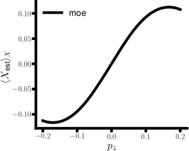
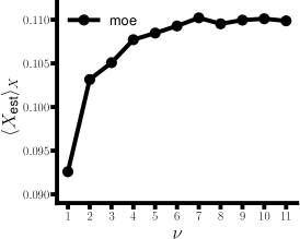
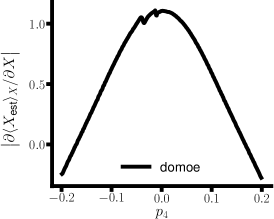
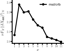
Figure S1: Additional results on maximum likelihood estimation, where “moe” is the mean of estimates ($\langle X_{\text{est}}\rangle_{X}$), “msd” is the mean-square deviation ($\langle(\delta X_{\text{est}})^{2}\rangle_{X}$), and “domoe” stands for the absolute value of the derivative of the mean of estimates ($\big{|}\partial\langle X_{\text{est}}\rangle_{X}/\partial X\big{|}$).

I.4.2 Further results on MLE statistics

Additional details on the MLE are supplied in Fig. S1 on the following page. The top left shows the mean of the maximum likelihood estimator with respect to the final state that has evolved under the true value of $p_{4}$. To calculate the mean, the probability distribution first needs to be composed. One measurement outcome is used at a single time of estimation, i.e., $\nu=1$. When the true value of $p_{4}$ is $0.1$, $\langle X_{\text{est}}\rangle_{X}\simeq 0.0926$. The top right plot shows the mean of the maximum likelihood estimator versus $\nu$ when $p_{4}=0.1$, which is the number of measurement outcomes for a single estimation of $p_{4}$. As $\nu$ increases, $\langle X_{\text{est}}\rangle_{X}$ converges at around $0.11$, which implies a bias of MLE. The bottom left shows this bias of the MLE, where $\big{|}\partial\langle X_{\text{est}}\rangle_{X}/\partial X\big{|}\simeq 1$ near $p_{4}\simeq 0$, which however does not hold as $p_{4}$ deviates more significantly from zero. Finally, the bottom right shows the ratio between the mean-square deviation and the Cramér-Rao lower bound (CRLB). This ratio decreases as $\nu$ increases: The MLE is known to make the mean-square deviation $\langle(\delta X_{\text{est}})^{2}\rangle_{X}$ converge to the CRLB as $\nu\rightarrow\infty$ according to the central limit theorem, which is thus confirmed.

References

- Helstrom [1967] C. W. Helstrom, Minimum mean-squared error of estimates in quantum statistics, Physics Letters A 25, 101 (1967).
- Helstrom [1969] C. W. Helstrom, Quantum detection and estimation theory, Journal of Statistical Physics 1, 231 (1969).
- Braunstein and Caves [1994] S. L. Braunstein and C. M. Caves, Statistical distance and the geometry of quantum states, Phys. Rev. Lett. 72, 3439 (1994).
- Braunstein et al. [1996] S. L. Braunstein, C. M. Caves, and G. Milburn, Generalized Uncertainty Relations: Theory, Examples, and Lorentz Invariance, Annals of Physics 247, 135 (1996).
- Giovannetti et al. [2006] V. Giovannetti, S. Lloyd, and L. Maccone, Quantum Metrology, Phys. Rev. Lett. 96, 010401 (2006).
- Wiseman and Milburn [2010] H. Wiseman and G. Milburn, Quantum Measurement and Control (Cambridge University Press, 2010).
- Tóth and Apellaniz [2014] G. Tóth and I. Apellaniz, Quantum metrology from a quantum information science perspective, Journal of Physics A: Mathematical and Theoretical 47, 424006 (2014).
- Braun et al. [2018] D. Braun, G. Adesso, F. Benatti, R. Floreanini, U. Marzolino, M. W. Mitchell, and S. Pirandola, Quantum-enhanced measurements without entanglement, Rev. Mod. Phys. 90, 035006 (2018).
- Schnabel et al. [2010] R. Schnabel, N. Mavalvala, D. E. McClelland, and P. K. Lam, Quantum metrology for gravitational wave astronomy, Nature Communications 1, 121 (2010).
- Braun et al. [2017] D. Braun, F. Schneiter, and U. R. Fischer, Intrinsic measurement errors for the speed of light in vacuum, Classical and Quantum Gravity 34, 175009 (2017).
- Giovannetti et al. [2011] V. Giovannetti, S. Lloyd, and L. Maccone, Advances in quantum metrology, Nature Photonics 5, 222 (2011).
- Pirandola et al. [2018] S. Pirandola, B. R. Bardhan, T. Gehring, C. Weedbrook, and S. Lloyd, Advances in photonic quantum sensing, Nature Photonics 12, 724 (2018).
- Polino et al. [2020] E. Polino, M. Valeri, N. Spagnolo, and F. Sciarrino, Photonic quantum metrology, AVS Quantum Science 2, 024703 (2020).
- Barbieri [2022] M. Barbieri, Optical Quantum Metrology, PRX Quantum 3, 010202 (2022).
- Pezzè et al. [2005] L. Pezzè, L. A. Collins, A. Smerzi, G. P. Berman, and A. R. Bishop, Sub-shot-noise phase sensitivity with a Bose-Einstein condensate Mach-Zehnder interferometer, Phys. Rev. A 72, 043612 (2005).
- Choi and Sundaram [2008] S. Choi and B. Sundaram, Bose-Einstein condensate as a nonlinear Ramsey interferometer operating beyond the Heisenberg limit, Phys. Rev. A 77, 053613 (2008).
- Boixo et al. [2009] S. Boixo, A. Datta, M. J. Davis, A. Shaji, A. B. Tacla, and C. M. Caves, Quantum-limited metrology and Bose-Einstein condensates, Phys. Rev. A 80, 032103 (2009).
- Gross et al. [2010] C. Gross, T. Zibold, E. Nicklas, J. Estève, and M. K. Oberthaler, Nonlinear atom interferometer surpasses classical precision limit, Nature 464, 1165 (2010).
- Chwedeńczuk et al. [2010] J. Chwedeńczuk, F. Piazza, and A. Smerzi, Phase estimation with interfering Bose-Einstein-condensed atomic clouds, Phys. Rev. A 82, 051601 (2010).
- Javanainen and Chen [2012] J. Javanainen and H. Chen, Optimal measurement precision of a nonlinear interferometer, Phys. Rev. A 85, 063605 (2012).
- Gross [2012] C. Gross, Spin squeezing, entanglement and quantum metrology with Bose–Einstein condensates, Journal of Physics B: Atomic, Molecular and Optical Physics 45, 103001 (2012).
- Berrada et al. [2013] T. Berrada, S. van Frank, R. Bücker, T. Schumm, J. F. Schaff, and J. Schmiedmayer, Integrated Mach–Zehnder interferometer for Bose–Einstein condensates, Nature Communications 4, 2077 (2013).
- Muessel et al. [2014] W. Muessel, H. Strobel, D. Linnemann, D. B. Hume, and M. K. Oberthaler, Scalable Spin Squeezing for Quantum-Enhanced Magnetometry with Bose-Einstein Condensates, Phys. Rev. Lett. 113, 103004 (2014).
- Strobel et al. [2014] H. Strobel, W. Muessel, D. Linnemann, T. Zibold, D. B. Hume, L. Pezzè, A. Smerzi, and M. K. Oberthaler, Fisher information and entanglement of non-Gaussian spin states, Science 345, 424 (2014).
- Gietka and Chwedeńczuk [2014] K. Gietka and J. Chwedeńczuk, Atom interferometer in a double-well potential, Phys. Rev. A 90, 063601 (2014).
- Huang et al. [2014] J. Huang, S. Wu, H. Zhong, and C. Lee, Quantum metrology with cold atoms, in Annual Review of Cold Atoms and Molecules (2014) Chap. 7, pp. 365–415.
- Ragole and Taylor [2016] S. Ragole and J. M. Taylor, Interacting Atomic Interferometry for Rotation Sensing Approaching the Heisenberg Limit, Phys. Rev. Lett. 117, 203002 (2016).
- Luo et al. [2017] C. Luo, J. Huang, X. Zhang, and C. Lee, Heisenberg-limited Sagnac interferometer with multiparticle states, Phys. Rev. A 95, 023608 (2017).
- Pezzè et al. [2018] L. Pezzè, A. Smerzi, M. K. Oberthaler, R. Schmied, and P. Treutlein, Quantum metrology with nonclassical states of atomic ensembles, Rev. Mod. Phys. 90, 035005 (2018), and the extensive list of references therein.
- Czajkowski et al. [2019] J. Czajkowski, K. Pawłowski, and R. Demkowicz-Dobrzański, Many-body effects in quantum metrology, New Journal of Physics 21, 053031 (2019).
- Szigeti et al. [2020] S. S. Szigeti, S. P. Nolan, J. D. Close, and S. A. Haine, High-Precision Quantum-Enhanced Gravimetry with a Bose-Einstein Condensate, Phys. Rev. Lett. 125, 100402 (2020).
- Streltsov et al. [2006] A. I. Streltsov, O. E. Alon, and L. S. Cederbaum, General variational many-body theory with complete self-consistency for trapped bosonic systems, Phys. Rev. A 73, 063626 (2006).
- Alon et al. [2008] O. E. Alon, A. I. Streltsov, and L. S. Cederbaum, Multiconfigurational time-dependent Hartree method for bosons: Many-body dynamics of bosonic systems, Phys. Rev. A 77, 033613 (2008).
- Lode et al. [2020] A. U. J. Lode, C. Lévêque, L. B. Madsen, A. I. Streltsov, and O. E. Alon, Colloquium: Multiconfigurational time-dependent Hartree approaches for indistinguishable particles, Rev. Mod. Phys. 92, 011001 (2020).
- Lin et al. [2020] R. Lin, P. Molignini, L. Papariello, M. C. Tsatsos, C. Lévêque, S. E. Weiner, E. Fasshauer, R. Chitra, and A. U. J. Lode, MCTDH-X: The multiconfigurational time-dependent Hartree method for indistinguishable particles software, Quantum Science and Technology 5, 024004 (2020).
- [36] The Supplemental Material, which quotes Refs. [51-53], contains a description of the MCTDH method and derivations of metrological quantities within the MCTDH framework, such as the quantum Fisher information, the probability distribution (likelihood), and details on the maximum likelihood estimator. Equation numbers quoted in the main text in the format (S#) refer to equations in the supplement.
- Fujiwara and Nagaoka [1995] A. Fujiwara and H. Nagaoka, Quantum Fisher metric and estimation for pure state models, Physics Letters A 201, 119 (1995).
- Barndorff-Nielsen and Gill [2000] O. E. Barndorff-Nielsen and R. D. Gill, Fisher information in quantum statistics, Journal of Physics A: Mathematical and General 33, 4481 (2000).
- Boixo et al. [2008] S. Boixo, A. Datta, S. T. Flammia, A. Shaji, E. Bagan, and C. M. Caves, Quantum-limited metrology with product states, Phys. Rev. A 77, 012317 (2008).
- Alipour et al. [2014] S. Alipour, M. Mehboudi, and A. T. Rezakhani, Quantum Metrology in Open Systems: Dissipative Cramér-Rao Bound, Phys. Rev. Lett. 112, 120405 (2014).
- Wasak et al. [2016] T. Wasak, A. Smerzi, L. Pezzè, and J. Chwedeńczuk, Optimal measurements in phase estimation: simple examples, Quantum Information Processing 15, 2231 (2016).
- Note [1] In , m yields a time unit msec.
- Olshaniǐ [1998] M. Olshaniǐ, Atomic Scattering in the Presence of an External Confinement and a Gas of Impenetrable Bosons, Phys. Rev. Lett. 81, 938 (1998).
- Baak and Fischer [2022] J.-G. Baak and U. R. Fischer, Classical and quantum metrology of the Lieb-Liniger model, Phys. Rev. A 106, 062442 (2022).
- Milburn et al. [1997] G. J. Milburn, J. Corney, E. M. Wright, and D. F. Walls, Quantum dynamics of an atomic Bose-Einstein condensate in a double-well potential, Phys. Rev. A 55, 4318 (1997).
- Alon and Cederbaum [2005] O. E. Alon and L. S. Cederbaum, Pathway from Condensation via Fragmentation to Fermionization of Cold Bosonic Systems, Phys. Rev. Lett. 95, 140402 (2005).
- Penrose and Onsager [1956] O. Penrose and L. Onsager, Bose-Einstein Condensation and Liquid Helium, Phys. Rev. 104, 576 (1956).
- Fisher [1922] R. A. Fisher, On the mathematical foundations of theoretical statistics, Philosophical Transactions of the Royal Society of London A 222, 309 (1922).
- Fisher [1925] R. A. Fisher, Theory of Statistical Estimation, Mathematical Proceedings of the Cambridge Philosophical Society 22, 700–725 (1925).
- Rossi [2018] R. Rossi, Mathematical Statistics: An Introduction to Likelihood Based Inference (Wiley, 2018).
- Lee and Fischer [2014] K.-S. Lee and U. R. Fischer, Truncated many-body dynamics of interacting bosons: A variational principle with error monitoring, International Journal of Modern Physics B 28, 1550021 (2014).
- Nijenhuis and Wilf [2014] A. Nijenhuis and H. Wilf, Combinatorial Algorithms: For Computers and Calculators, edited by W. Rheinboldt, Computer science and applied mathematics (Elsevier Science, 2014).
- Niu et al. [2020] X. Niu, S. Su, and J. Zheng, A New Fast Computation of a Permanent, IOP Conference Series: Materials Science and Engineering 790, 012057 (2020).