Practical, Private Assurance of the Value of Collaboration

Abstract

Two parties wish to collaborate on their datasets. However, before they reveal their datasets to each other, the parties want to have the guarantee that the collaboration would be fruitful. We look at this problem from the point of view of machine learning, where one party is promised an improvement on its prediction model by incorporating data from the other party. The parties would only wish to collaborate further if the updated model shows an improvement in accuracy. Before this is ascertained, the two parties would not want to disclose their models and datasets. In this work, we construct an interactive protocol for this problem based on the fully homomorphic encryption scheme over the Torus (TFHE) and label differential privacy, where the underlying machine learning model is a neural network. Label differential privacy is used to ensure that computations are not done entirely in the encrypted domain, which is a significant bottleneck for neural network training according to the current state-of-the-art FHE implementations. We prove the security of our scheme in the universal composability framework assuming honest-but-curious parties, but where one party may not have any expertise in labelling its initial dataset. Experiments show that we can obtain the output, i.e., the accuracy of the updated model, with time many orders of magnitude faster than a protocol using entirely FHE operations.

1 Introduction

Data collaboration, i.e., joining multiple datasets held by different parties, can be mutually beneficial to all parties involved as the joint dataset is likely to be more representative of the population than its constituents. In the real world, parties have little to no knowledge of each others’ datasets before collaboration. Arguably, the parties would only collaborate if they had some level of trust in the quality of data held by other parties. When the parties involved are reputable organizations, one may assume their datasets to be of high quality. However, in many cases, little may be known about them. In such cases, each party would like some sort of assurance that their collaboration will indeed be beneficial.

Let us elaborate this scenario with an example. Assume companies $P_{1}$ and $P_{2}$ are in the business of developing antivirus products. Each company holds a dataset of malware programs labelled as a particular type of malware, e.g., ransomware, spyware and trojan. This labelling is done by a team of human experts employed by the company. Since manual labelling is expensive, $P_{1}$ uses a machine learning model to label new malware programs. The performance of this model can be tested against a smaller holdout dataset of the latest malware programs labelled by the same experts. However, due to a number of reasons such as the under-representation of some of the malware classes in the training dataset or concept drift [1] between the training dataset and the holdout dataset, the performance of this model on the holdout dataset begs improvement. Company $P_{2}$ offers a solution: by combining $P_{2}$’s dataset with $P_{1}$’s, the resulting dataset would be more representative and hence would improve the accuracy of $P_{1}$’s model. Before going into the laborious process of a formal collaborative agreement with $P_{2}$, $P_{1}$ would like to know whether this claim will indeed be true. On the other hand, $P_{2}$ would not want to hand over its dataset, in particular, its labels to $P_{1}$ before the formal agreement.

Many similar examples to the one outlined above may occur in real-world data collaboration scenarios. A rather straightforward solution to this problem can be obtained using fully homomorphic encryption (FHE). Party $P_{2}$ encrypts the labels of its dataset using the encryption function of the FHE scheme, and sends its dataset with encrypted labels to $P_{1}$. Party $P_{1}$, then combines this dataset with its own, trains the model and tests its accuracy against the holdout dataset all using FHE operations. The final output is then decrypted by party $P_{2}$. However, this involves training the model entirely in the encrypted domain, which even with the state-of-the-art homomorphic encryption schemes, is computationally expensive [2, 3, 4, 5, 6].

In this paper, we propose an efficient solution to this problem. We combine fully homomorphic encryption over the torus [7] with label differential privacy [8] to provide an interactive solution where $P_{2}$ can use a specific value of the differentially privacy parameter $\epsilon$ such that the accuracy of the model on the joint datasets lies between the accuracy of $P_{1}$’s model and the accuracy achievable on the joint model if no differential privacy were to be applied. This provides assurance to $P_{1}$ that the combined dataset will improve accuracy promising further improvement if the parties combine their datasets in the clear via the formal collaborative agreement. Our main idea is that since the features are known in the clear, the first forward pass in the backpropagation algorithm of neural networks can be performed in the clear, up to the point where we utilize the (encrypted) labels from party $P_{2}$’s dataset. If further computation is done homomorphically, then we would endure the same computational performance bottleneck as previous work. We, therefore, add (label) differentially private noise to the gradients and decrypt them before the backward pass. This ensures that most steps in the neural network training are done in cleartext, albeit with differentially private noise, giving us computational performance improvements over an end-to-end FHE solution. In what follows, we first formally show that without domain knowledge it is not possible for $P_{2}$ to improve the model accuracy. We then describe our protocol in detail, followed by its privacy and security analysis. Finally, we evaluate the performance and accuracy of our protocol on multiple datasets.

2 Preliminaries and Threat Model

2.1 Notation

We follow the notations introduced in [9]. The datasets come from the joint domain: $\mathbb{D}=\mathcal{X}\times\mathcal{Y}$, where $\mathcal{X}$ denotes the domain of features, and $\mathcal{Y}$ denotes the domain of labels. A dataset $D$ is a multiset of elements drawn i.i.d. from the domain under the joint distribution $\mathcal{D}$ over domain points and labels. We denote by $\mathcal{D}_{x}$, the marginal distribution of unlabelled domain points. In some cases, a dataset may be constructed by drawing unlabelled domain points under $\mathcal{D}_{x}$, and then labelled according to some labelling function, which may not follow the marginal distribution of labels under $\mathcal{D}$, denoted $\mathcal{D}_{y|x}$. In such a case, we shall say that the dataset is labelled by the labelling function to distinguish it from typical datasets. Let $\mathcal{A}$ denote the learning algorithm, e.g., a neural network training algorithm. We denote by $M\leftarrow\mathcal{A}(D)$ the model $M$ returned by the learning algorithm on dataset $D$. Given the model $M$, and a sample $(x,y)\leftarrow\mathcal{D}$, we define a generic loss function $\ell(M,x,y)$, which outputs a non-negative real number. For instance, $\ell(M,x,y)$ can be the 0-1 loss function, defined as:

$$\ell(M,x,y)=\begin{cases}1,\text{ if }M(x)\neq y\\ 0,\text{ otherwise}\end{cases}$$

We define the true error of $M$ as

$$L_{\mathcal{D}}(M)=\mathbb{E}_{(x,y)\sim\mathcal{D}}[\ell(M,x,y)].$$

Notice that for the 0-1 loss function, this means that

$$L_{\mathcal{D}}(M)=\Pr_{(x,y)\sim\mathcal{D}}[M(x)\neq y]$$

The empirical error of the model $M$ over the dataset $D$ having $m$ elements $(x_{1},y_{1}),\ldots,(x_{m},y_{m})$ is defined as:

$$L_{D}(M)=\frac{1}{m}\sum_{i\in[m]}\ell(M,x_{i},y_{i})$$ (1)

2.2 The Setting

The Scenario. We consider two parties $P_{1}$ and $P_{2}$. For $i\in\{1,2\}$, party $P_{i}$’s dataset is denoted $D_{i}$. Each $D_{i}$ contains points of the form $(\mathbf{x},y)$. The parties wish to collaborate on their datasets $D_{i}$. The features $\mathbf{x}$ are shared in the open; whereas the labels $y$ for each $\mathbf{x}$ in $D_{i}$ are to be kept secret from the other party. This scenario holds in applications where gathering data ($\mathbf{x}$) may be easy, but labelling is expensive. For example, malware datasets (binaries of malware programs) are generally available to antivirus vendors, and often times features are extracted from these binaries using publicly known feature extraction techniques, such as the LIEF project [10]. However, labelling them with appropriate labels requires considerable work from (human) experts. Other examples include sentiment analysis on public social media posts, and situations where demographic information is public (e.g., census data) but income predictability is private [8].

The Model. Before the two parties reveal their datasets to each other, the parties want to have the guarantee that the collaboration would be valuable. We shall assume that party $P_{1}$ already has a model $M_{1}$ trained on data $D_{1}$. $P_{1}$ also has a labelled holdout data $D_{\text{hold}}$ against which $P_{1}$ tests the accuracy of $M_{1}$. The goal of the interaction is to obtain a new model $M_{2}$ trained on $D_{1}\cup D_{2}$. $M_{2}$’s accuracy again is tested against $D_{\text{hold}}$. The collaboration is defined to be valuable for $P_{1}$ if the accuracy of $M_{2}$ is higher than the accuracy of $M_{1}$ against $D_{\text{hold}}$. In this paper, we only study value from $P_{1}$’s perspective. We will consider a neural network trained via stochastic gradient descent as our canonical model.

The Holdout Dataset. As mentioned above, $P_{1}$ has a holdout dataset $D_{\text{hold}}$ against which the accuracy of the models is evaluated. This is kept separate from the usual training-testing split of the dataset $D_{1}$. It makes sense to keep the same holdout dataset to check how the model trained on the augmented/collaborated data performs. For instance, in many machine learning competitions teams compete by training their machine learning models on a publicly available training dataset, but the final ranking of the models, known as private leaderboard, is done on a hidden test dataset [11]. This ensures that the models are not overfitted by using the test dataset as feedback for re-training. We assume that $D_{\text{hold}}$ is continually updated by adding new samples (e.g., malware never seen by $P_{1}$) labelled by human experts, and is more representative of the population than $D_{1}$. For instance, the holdout dataset reflects the concept drift [1] better than $D_{1}$. If $D_{2}$ happens to have the same concept drift as $D_{\text{hold}}$, then $M_{2}$ (trained on $D_{1}\cup D_{2}$) would have better test accuracy than $M_{1}$ against $D_{\text{hold}}$. Alternatively, the holdout dataset could be more balanced than $D_{1}$, e.g., if $D_{1}$ has labels heavily skewed towards one class. Again, in this case, if $D_{2}$ is more balanced than $D_{1}$, then $M_{2}$ will show better accuracy. We argue that it is easy for $P_{1}$ to update $D_{\text{hold}}$ than $D_{1}$ as the latter requires more resources due to the difference in size.

2.3 Privacy

Privacy Expectations. We target the following privacy properties:

• Datasets $D_{1}$ and $D_{\text{hold}}$, and model $M_{1}$ should be hidden from $P_{2}$.

• The labels of dataset $D_{2}$ should be hidden from $P_{1}$.

• Neither $P_{1}$ nor $P_{2}$ should learn $M_{2}$, i.e., the model trained on $D_{1}\cup D_{2}$.

• Both parties should learn whether ${L}_{\text{hold}}(M_{2})<{L}_{\text{hold}}(M_{1})$, where ${L}_{\text{hold}}$ is the loss evaluated on $D_{\text{hold}}$ (see Eq. (1)).

Threat Model. We assume that the parties involved, $P_{1}$ and $P_{2}$, are honest-but-curious. This is a reasonable assumption since once collaboration is agreed upon, the model trained on clear data should be able to reproduce any tests to assess the quality of data pre-agreement. Why then would $P_{1}$ not trust the labelling from $P_{2}$? This could be due to the low quality of $P_{2}$’s labels, for many reasons. For example, $P_{2}$’s expertise could in reality be below par. In this case, even though the labelling is done honestly, it may not be of sufficient quality. Furthermore, $P_{2}$ can in fact lie about faithfully doing its labelling without the fear of being caught. This is due to the fact that technically there is no means available to $P_{1}$ to assess how $P_{2}$’s labels were produced. All $P_{2}$ needs to do is to provide the same labels before and after the collaborative agreement. As long as labelling is consistent, there is no fear of being caught.

2.4 Background

Feedforward Neural Networks. A fully connected feedforward neural network is modelled as a graph with a set of vertices (neurons) organised into layers and weighted edges connecting vertices in adjacent layers. The sets of vertices from each layer form a disjoint set. There are at least three layers in a neural network, one input layer, one or more hidden layers and one output layer. The number of neurons in the input layer equals the number of features (dimensions). The number of neurons in the output layer is equal to the number of classes $K$. The vector of weights $\mathbf{w}$ of all the weights of the edges constitutes the parameters of the network, to be learnt during training. We let $R$ denote the number of weights in the last layer, i.e., the number of edges connecting to the neurons in the output layer. For a more detailed description of neural networks, see [9].

Backward Propagation and Loss. Training a deep neural network involves multiple iterations/epochs of forward and backward propagation. The input to each neuron is the weighted sum of the outputs of all neurons connected to it (from the previous layer), where the weights are associated with the edge connecting to the current neuron. The output of the neuron is the application of the activation function on this input. In this paper, we assume the activation function to be the sigmoid function. Let $\mathbf{z}=\begin{pmatrix}z_{1},z_{2},\ldots,z_{K}\end{pmatrix}$ denote the output of the last layer of the neural network. We assume there to be a softmax layer, immediately succeeding this which outputs the probability vector $\mathbf{p}$, whose individual components are given as $p_{i}={e^{z_{i}}}/(\sum_{j}e^{z_{j}})$. Clearly, the sum of these probabilities is 1. Given the one-hot encoded label $\mathbf{y}$, one can compute the loss as $L(\mathbf{w})=\sum_{i=1}^{K}\ell(p_{i},y_{i})$, where $\ell(\cdot,\cdot)$ is the loss function. In this paper, we shall consider it to be the cross-entropy loss given by: $\ell(p_{i},y_{i})=-\sum_{i=1}^{K}y_{i}\ln p_{i}$. Given $L(\mathbf{w})$, we can calculate its gradient as:

$$\nabla L(\mathbf{w})=\frac{\partial L}{\partial\mathbf{w}}=\frac{\partial L}{\partial\mathbf{p}}\frac{\partial\mathbf{p}}{\partial\mathbf{z}}\frac{\partial\mathbf{z}}{\partial\mathbf{w}}$$

This chain rule can be used in the backpropagation algorithm to calculate the gradients to minimise the loss function via stochastic gradient descent (SGD). The calculated gradients will be then used to update the weights associated with each edge for the forward propagation in the next epoch. For more details of the backpropagation-based SGD algorithm, see [9].

Label Differential Privacy. Since only the labels of the dataset $D_{2}$ are needed to be private, we shall use the notion of label differential privacy to protect them. Ordinary differential privacy [12] defines neighbouring datasets as a pair of datasets which differ in one row. Label differential privacy considers two datasets of the same length as being neighbours if they differ only in the label of exactly one row [8]. This is a suitable definition of privacy for many machine learning applications such as malware labels (as already discussed) and datasets where demographic information is already public but some sensitive feature (e.g., income) needs to be protected [8]. Furthermore, for tighter privacy budget analysis we use the notion of $f$-differential privacy [13], modified for label privacy since it allows straightforward composition of the Gaussian mechanism as opposed to the normal definition of differential privacy which needs to invoke its approximate variant to handle this mechanism. More formally, two datasets $D_{1}$ and $D_{2}$ are said to be neighbouring datasets, if they are of the same size and differ only in at most one label.

The $f$-differential privacy framework is based on the hypothesis testing interpretation of differential privacy. Given the output of the mechanism $\mathcal{A}$, the goal is to distinguish between two competing hypotheses: the underlying data set being $D_{1}$ or $D_{2}$. Let $Q_{1}$ and $Q_{2}$ denote the probability distributions of $\mathcal{A}(D_{1})$ and $\mathcal{A}(D_{2})$, respectively. Given any rejection rule $0\leq\phi\leq 1$, the type-I and type-II errors are defined as follows  [13]: $\alpha_{\phi}=\mathbb{E}_{Q_{1}}[\phi]$ and $\beta_{\phi}=1-\mathbb{E}_{Q_{2}}[\phi]$.

Definition 1 (Trade-off function [13]).

For any two probability distributions $Q_{1}$ and $Q_{2}$ on the same space, the trade-off function $T(Q_{1},Q_{2}):[0,1]\to[0,1]$ is defined by

$$T(Q_{1},Q_{2})(\alpha)=\inf\{\beta_{\phi}:\alpha_{\phi}\leq\alpha\}$$

for all $\alpha\in[0,1]$, where the infimum is taken over all (measurable) rejection rules.

A trade-off function gives the minimum achievable type-II error at any given level of type-I error. For a function to be a trade-off function, it must satisfy the following conditions.

Proposition 1 ([13]).

A function $f:[0,1]\to[0,1]$ is a trade-off function if and only if $f$ is convex, continuous and non-increasing, and $f(x)\leq 1-x$ for all $x\in[0,1]$.

Abusing notation, let $\mathcal{A}(D)$ denote the distribution of a mechanism $\mathcal{A}$ when given a data set $D$ as input. We now give a definition of $f$-label differential privacy based on the definition of ordinary $f$-differential privacy:

Definition 2 ($f$-Label Differential Privacy [13]).

Let $f$ be a trade-off function. A mechanism $\mathcal{A}$ is said to be $f$-label differentially private if $T(\mathcal{A}(D_{1}),\mathcal{A}(D_{2}))\geq f$ for all neighbouring data sets $D_{1}$ and $D_{2}$.

Note that the only change here from the definition of $f$-differential privacy from [13] is how we define neighbouring datasets. In our case neighbouring datasets differ only in the label of at most one sample. We now give a concrete $f$-label differentially private mechanism.

Proposition 2 ($\epsilon$-Gaussian Label Differential Privacy [13]).

The mechanism $q(D)+\mathcal{N}(0,\Delta q^{2}/\epsilon^{2})$ is $\epsilon$-GLDP where $\Delta q$ is the sensitivity of the function $q$ over any pairs of neighbouring (in label) datasets $D_{1}$ and $D_{2}$.

The notion of $\epsilon$-GLDP satisfies both sequential and parallel composition.

Proposition 3 (Sequential and Parallel Composition).

The composition of $n$-fold (sequential) $\epsilon_{i}$-GLDP mechanisms is $\sqrt{\epsilon_{1}^{2}+\cdots+\epsilon_{n}^{2}}$-GLDP [13]. Let a sequence of $n$ mechanisms $\mathcal{A}_{i}$ each be $\epsilon_{i}$-GLDP. Let $\mathbb{D}_{i}$ be disjoint subsets of the data domain $\mathbb{D}$. The joint mechanism defined as the sequence of $\mathcal{A}_{i}(D\cap\mathbb{D}_{i})$ (given also the output of the previous $i-1$ mechanisms) is $\max\{\epsilon_{1},\ldots,\epsilon_{n}\}$-GLDP [14].

Lastly, $f$-differential privacy is also immune to post-processing [13]. That is, applying a randomised map with an arbitrary range to the output of an $f$-label differentially private algorithm maintains $f$-label differential privacy.

Fully Homomorphic Encryption over the Torus (TFHE). Let $\mathbb{T}$ denote the torus, the set of real numbers modulo 1, i.e., the set $[0,1)$. The torus defines an Abelian group where two elements can be added modulo 1. The internal product is not defined. However, one can multiply an integer with a torus element by simply multiplying them in a usual way and reducing modulo 1. For a positive integer $q$, the discretised torus $\mathbb{T}_{q}$ is defined as the set $\{0,\frac{1}{q},\ldots,\frac{q-1}{q}\}$. Clearly $\mathbb{T}_{q}\subset\mathbb{T}$. Given elements $\frac{a}{q},\frac{b}{q}\in\mathbb{T}_{q}$, their sum is $\frac{c}{q}\in\mathbb{T}_{q}$, where $c\equiv a+b\pmod{q}$. Given an integer $z\in\mathbb{Z}$ and a torus element $\frac{a}{q}\in\mathbb{T}_{q}$, we define their product $z\cdot\frac{a}{q}$ as $\frac{b}{q}$ where $b\equiv za\pmod{q}$. The plaintext space is a subgroup of $\mathbb{T}_{q}$, defined as $\mathcal{P}=\{0,\frac{1}{p},\ldots,\frac{p-1}{p}\}$, for some $p\geq 2$ such that $p$ divides $q$.

Let $\chi$ be the normal distribution $\mathcal{N}(0,\sigma^{2})$ over $\mathbb{R}$. Let $e_{0}\leftarrow\chi$. The noise error $e\in\hat{\chi}$ is defined as

$$e=\frac{\lfloor qe_{0}\rceil}{q}$$

Let $N$ be a positive integer. Let $\mathbf{s}=(s_{1},\ldots,s_{N})$ be a binary vector chosen uniformly at random (the private key). Given a message $x\in\mathcal{P}$, the TLWE encryption of $x$ under $\mathbf{s}$ is defined as $\mathbf{c}=(\mathbf{a},b)\in\mathbb{T}_{q}^{N+1}$, where $\mathbf{a}$ is a vector of $N$-elements drawn uniformly at random from $\mathbb{T}_{q}$, and

$$b=\langle\mathbf{s},\mathbf{a}\rangle+x+e.$$

To decrypt $\mathbf{c}$ one computes: $x^{*}=b-\langle\mathbf{s},\mathbf{a}\rangle$, and returns the nearest element in $\mathcal{P}$ to $x^{*}$. The scheme is secure under the learning with errors (LWE) problem over the discretized torus [7, 15]:

Definition 3 (TLWE Assumption).

Let $q,N\in\mathbf{N}$. Let $\mathbf{s}=(s_{1},\ldots,s_{N})$ be a binary vector chosen uniformly at random. Let $\hat{\chi}$ be an error distribution defined above. The learning with errors over the discretized torus (TLWE) problem is to distinguish samples chosen according to the following distributions:

$$\mathcal{D}_{0}=\{(\mathbf{a},b)\mid\mathbf{a}\leftarrow\mathbb{T}_{q}^{N},b\leftarrow\mathbb{T}_{q}\},$$

and

$$\mathcal{D}_{1}=\{(\mathbf{a},b)\mid\mathbf{a}\leftarrow\mathbb{T}_{q}^{N},b=\langle\mathbf{s},\mathbf{a}\rangle+e,e\leftarrow\hat{\chi}\},$$

where except for $e$ which is sample according to the distribution $\hat{\chi}$, the rest are sampled uniformly at random from the respective sets.

Integer Encoding. Before encrypting, we will encode the input as an integer. This is a requirement in the current version of Zama’s Concrete TFHE library [16], which we use for our implementation. Let $\mathbf{x}\in\mathbb{R}^{m}$. For a precision level $r$, where $r$ is a positive integer, we will encode $\mathbf{x}$ as $\lfloor r\mathbf{x}\rfloor=(\lfloor rx_{1}\rfloor,\ldots,\lfloor rx_{m}\rfloor)$, before encrypting. Decoding is done, after decryption, by dividing the encoded vector by $r$. For instance if $r=10$, then the real number $3.456$ is encoded as $\lfloor 34.56\rfloor=34$. Decoding it yields $3.4$.

Parameters. We use the default parameters for TLWE encryption available through the Concrete library. Under the default setting, we have $N=630$, giving us a security level of 128 bits. The parameter $q$ is set to 64 bits, meaning a torus element can be represented by 64 bits [15]. Since the plaintext parameter $p$ divides $q$, we can assume $p$ to be less than 64 bits. The noise parameter $\sigma$ is $2^{-15}$ [15].

3 Lack of Domain Knowledge

Before we give a privacy-preserving solution to our problem, we want to show that the problem does indeed have a solution in the clear domain. More precisely, we show that if party $P_{2}$ lacks domain knowledge, then the party cannot come up with a dataset $D_{2}$ such that ${L}_{\text{hold}}(M_{2})<{L}_{\text{hold}}(M_{1})$, where $M_{2}\leftarrow\mathcal{A}(D_{1}\cup D_{2})$ and $M_{1}\leftarrow\mathcal{A}(D_{1})$, where $L_{\text{hold}}$ is as defined in Eq. (1). For simplicity we assume binary classification, although the results can be easily extended to multiclass classification. We also assume the 0-1 loss function. How do we define lack of domain knowledge? Since the feature vectors are public, $P_{2}$ can easily obtain a set of raw inputs to obtain the feature vectors in $D_{2}$. Thus, domain knowledge should be captured in the labels to the feature vectors in $D_{2}$. We define lack of domain knowledge as using a labeling function $g$ which labels any domain point $x$ independent of the distribution of its true label. That is given any $x\in\mathcal{X}$:

$$\Pr[g(x)=y^{\prime}\mid\mathcal{D}_{y|x}]=\Pr[g(x)=y^{\prime}],$$ (2)

for all $y^{\prime}\in\mathcal{Y}$. Note that this does not mean that the labeling is necessarily incorrect. We call $g$ as defined in Eq. 2 as an oblivious labeling function. We shall first show that if $D$ is labelled by an oblivious labeling function, then $M$ as returned by a learning algorithm $\mathcal{A}$ (taking $D$ as the input) will have:

$${L}_{\text{hold}}(M)=1/2,$$

provided that $D_{\text{hold}}$ is a balanced dataset. Having established the necessity of $D_{\text{hold}}$ to be balanced, we shall then show that

$${L}_{\text{hold}}(M_{2})\geq{L}_{\text{hold}}(M_{1}),$$

where $M_{2}\leftarrow\mathcal{A}(D_{1}\cup D_{2})$, and $M_{1}\leftarrow\mathcal{A}(D_{1})$.

Theorem 1.

Let $D_{\text{hold}}$ be a balanced dataset. That is $\Pr[y=1\mid(x,y)\sim D_{\text{hold}}]=\frac{1}{2}$, where $\sim$ denotes uniform random sampling. Let $D$ be a dataset labelled by an oblivious labeling function $g$. Let $\mathcal{A}$ be a learning algorithm. Let $M\leftarrow\mathcal{A}(D)$. Then,

$${L}_{\text{hold}}(M)=1/2.$$

Proof.

See Appendix A ∎

What happens if $D_{\text{hold}}$ is not balanced? Then, we may get a loss less than $1/2$. To see this, assume that $\Pr[y=1\mid(x,y)\sim D_{\text{hold}}]=q>\frac{1}{2}$. Consider the oblivious labelling function $g$ which outputs 1 with probability $p=1$, i.e., the constant function $g(x)=1$. Then if $M$ is the Bayes optimal classifier [9, §3.2.1] for $g$, we have:

$$\Pr[M(x)\neq y] =\Pr[M(x)=0\mid y=1]\Pr[y=1]$$

$$+\Pr[M(x)=1\mid y=0]\Pr[y=0]$$

$$=\Pr[M(x)=1\mid y=0]\Pr[y=0]$$

$$=\Pr[y=0]=1-q<\frac{1}{2}.$$

Thus, it is crucial to test the model over a balanced dataset.

Theorem 2.

Let $D_{1}$ be a dataset. Let $D_{2}$ be a dataset labelled according to an oblivious labeling function $g$. Let $D_{\text{hold}}$ be a balanced dataset. Let $\mathcal{A}$ be a learning algorithm. Let $M_{1}\leftarrow\mathcal{A}(D_{1})$ and $M_{2}\leftarrow\mathcal{A}(D_{1}\cup D_{2})$. Then,

$${L}_{\text{hold}}(M_{2})\geq{L}_{\text{hold}}(M_{1})$$

Proof.

See Appendix A. ∎

4 Our Solution

4.1 Intuition

Figure 1: A batch will contain some points from $D_{1}$ and some from $D_{2}$. Only the labels from the points in $D_{2}$ needs to be kept private (shaded black) from $P_{1}$.

Consider the training of the neural network on $D_{1}\cup D_{2}$, with weights $\mathbf{w}$. Using the stochastic gradient descent (SGD) algorithm, one samples a batch $B$, from which we calculate per sample loss $L_{s}(\mathbf{w})$, where $s=(\mathbf{x},\mathbf{y})\in B$. Given this, we can compute the average loss over the batch via:

$$L_{B}(\mathbf{w})=\frac{1}{|B|}\sum_{s\in B}L_{s}(\mathbf{w})=\frac{1}{|B|}\sum_{\begin{subarray}{c}s\in B\\ s\in D_{1}\end{subarray}}L_{s}(\mathbf{w})+\frac{1}{|B|}\sum_{\begin{subarray}{c}s\in B\\ s\in D_{2}\end{subarray}}L_{s}(\mathbf{w})$$ (3)

As shown in Figure 1, everything in this computation is known to $P_{1}$, except for the labels in $D_{2}$. Thus, $P_{1}$ can compute the gradients for samples in $D_{1}$, but to update the weights, $P_{1}$ needs the gradients for samples from $D_{2}$. From Eq. (3), we are interested in computing the loss through the samples in a batch $B$ that belong to the dataset $D_{2}$. Overloading notation, we still use $B$ to denote the samples belonging to $D_{2}$. The algorithm to minimize the loss is the stochastic gradient descent algorithm using backpropagation. This inolves calculating the gradient $\nabla L_{B}(\mathbf{w})$. As noted in [17], if we are using the backpropagation algorithm, we only need to be concerned about the gradients corresponding to the last layer. Again, to simplify notation, we denote the vector of weights in the last layer by $\mathbf{w}$.

In Appendix B, we show that the gradient of the loss can be computed as:

$$\nabla L_{B}(\mathbf{w})=\frac{1}{|B|}\sum_{s\in B}\sum_{i=1}^{K}p_{i}(s)\frac{\partial z_{i}(s)}{\partial\mathbf{w}}-\frac{1}{|B|}\sum_{s\in B}\sum_{i=1}^{K}y_{i}(s)\frac{\partial z_{i}(s)}{\partial\mathbf{w}},$$ (4)

where $y_{i}(s)$ is the $i$th label of the sample $s$, $p_{i}(s)$ is the probability of the $i$th label of sample $s$, $z_{i}(s)$ is the $i$th input to the softmax function for the sample $s$, and $K$ denotes the number of classes. The LHS term of this equation can be computed by $P_{1}$ as this is in the clear. However, the RHS term requires access to the labels.

If we encrypt the labels, the gradients calculated in Eq. (4) will be encrypted, using the homomorphic property of the encryption scheme. This means that the gradient of the batch, as well as the weight updates will be encrypted. Thus, the entire training process after the first forward pass of the first epoch will be in the encrypted domain. While this presents one solution to our problem, i.e., obtaining an encrypted trained model, which could then be decrypted once the two parties wish to collaborate, existing line of works [2, 3, 4, 5, 6] show that neural network training entirely in the encrypted domain is highly inefficient. For instance, a single mini-batch of 60 samples can take anywhere from more than 30 seconds to several days with dedicated memory ranging from 16GB to 250GB using functional encryption or homomorphic encryption [6]. In some of our neural network implementations, we use a batch size of 128 with 100 epochs, which means that the time consumed for an end-to-end training entirely in the encrypted domain would be prohibitive. Our idea is to take advantage of the fact that the feature vectors are in the clear, and hence it may be possible to decrypt the labels in each batch so that backpropagation can be carried out in cleartext, giving us computational advantage over an all encrypted solution. This is where we employ label differential privacy. A straightforward way to accomplish this is to let $P_{2}$ add differentially private noise to all its labels and simply handover its noisy dataset to $P_{1}$, playing no further part (except for receiving the accuracy result). However, this is less desirable from the utility point of view as we argue in detail in Section 6.4. Instead, we add noise to the gradients in each batch with $P_{2}$ interactively adding noise to the average gradient computed in each epoch, similar to what is done in [17].

4.2 Proposed Protocol

Our solution is as follows.

1. To start, $P_{2}$ sends only the encrypted form of its dataset $D_{2}$ where each sample is $(\mathbf{x},\llbracket\mathbf{y}\rrbracket_{\mathsf{k}})$, where $\mathsf{k}$ is $P_{2}$’s encryption key of a homomorphic encryption scheme. In particular, $\llbracket\mathbf{y}\rrbracket_{\mathsf{k}}$ is a vector of $K$ elements, each element of which is encrypted under $\mathsf{k}$.

2. For each sample $s\in B$ and $1\leq i\leq K$, $P_{1}$ computes $\frac{\partial z_{i}(s)}{\partial\mathbf{w}}$. This results in $K\times|B|$ vectors of $R$-elements each, where $R$ is the number of weights in the last layer.

3. For each sample $s\in B$ and $1\leq i\leq K$, $P_{1}$ does element-wise homomorphic scalar multiplication: $\frac{\partial z_{i}(s)}{\partial\mathbf{w}}\llbracket y_{i}(s)\rrbracket_{\mathsf{k}}=\llbracket y_{i}(s)\lfloor r\frac{\partial z_{i}(s)}{\partial\mathbf{w}}\rfloor\rrbracket_{\mathsf{k}}$, where $r$ is the precision parameter. This amounts to a total of $K\times|B|\times R$ homomorphic scalar multiplications.

4. $P_{1}$ homomorphically adds:

   $$\sum_{s\in B}\sum_{i=1}^{K}\left\llbracket y_{i}(s)\left\lfloor r\frac{\partial z_{i}(s)}{\partial\mathbf{w}}\right\rfloor\right\rrbracket_{\mathsf{k}}$$

   $$= \left\llbracket\sum_{s\in B}\sum_{i=1}^{K}y_{i}(s)\left\lfloor r\frac{\partial z_{i}(s)}{\partial\mathbf{w}}\right\rfloor\right\rrbracket_{\mathsf{k}}=\left\llbracket N_{B}(\mathbf{w})\right\rrbracket_{\mathsf{k}},$$ (5)

   which amounts to a total of $K\times|B|\times R$ homomorphic additions. This results in an $R$-element vector encrypted under $\mathsf{k}$.

5. $P_{1}$ computes the sensitivity of the gradients of the loss function for the current batch. As shown in Appendix C this is $r\Delta S_{B}(\mathbf{w})$, where:

   $$\Delta S_{B}(\mathbf{w})=\frac{2}{|B|}\max_{i,s}\left\lVert\frac{\partial z_{i}(s)}{\partial\mathbf{w}}\right\rVert_{2},$$ (6)

   is the sensitivity of the gradients without encoding.

6. $P_{2}$ computes $R$-dimensional Gaussian noise vector $\mathcal{N}(0,\sigma^{2}\mathbf{1}_{R})$, where $\sigma=1/\epsilon$ and $\mathbf{1}_{R}$ is a vector of $R$ $1$’s. For each value $s$ in the list of allowable values of sensitivity of size $t$ (see below), $P_{2}$ updates the noise as $rs\mathcal{N}(0,\sigma^{2}\mathbf{1}_{R})=\mathcal{N}(0,(rs\sigma)^{2}\mathbf{1}_{R})$, and sends $\left\llbracket\lfloor\mathcal{N}(0,(rs\sigma)^{2}\mathbf{1}_{R})\rfloor\right\rrbracket_{\mathsf{k}}$ to $P_{1}$.

7. $P_{1}$ looks up the index of the smallest allowable sensitivity $s$ such that $\Delta S_{B}(\mathbf{w})\leq s$. $P_{1}$ then chooses the noise vector $\left\llbracket\lfloor\mathcal{N}(0,(rs\sigma)^{2}\mathbf{1}_{R})\rfloor\right\rrbracket_{\mathsf{k}}$ corresponding to this index as sent by $P_{2}$.

8. $P_{1}$ “blinds” the encrypted quantity $\left\llbracket N_{B}(\mathbf{w})\right\rrbracket_{\mathsf{k}}$ resulting in $\left\llbracket N_{B}(\mathbf{w})+\boldsymbol{\mu}\right\rrbracket_{\mathsf{k}}$ (see below). $P_{1}$ homomorphically adds the scaled noise vector and sends the following to $P_{2}$:

   $$\left\llbracket N_{B}(\mathbf{w})+\boldsymbol{\mu}+\lfloor\mathcal{N}(0,(rs\sigma)^{2}\mathbf{1}_{R})\rfloor\right\rrbracket_{\mathsf{k}}$$ (7)

9. $P_{2}$ decrypts the ciphertext and sends the following to $P_{1}$

   $$N_{B}(\mathbf{w})+\boldsymbol{\mu}+\lfloor\mathcal{N}(0,(rs\sigma)^{2}\mathbf{1}_{R})\rfloor$$ (8)

10. $P_{1}$ substracts $\mu$ and obtains $N_{B}(\mathbf{w})+\lfloor\mathcal{N}(0,(rs\sigma)^{2}\mathbf{1}_{R})\rfloor$. $P_{1}$ decodes this by dividing by $r$, plugs this into Equation (4) and proceeds with backgpropagation in the unencrypted domain.

Remark 1.

The parameter $R$, i.e., the number of weights in the last layer is being leaked here. We assume that this quantity, along with the batch size and the number of epochs are known by party $P_{2}$.

Adding a Random Blind. The labels are encrypted under party $P_{2}$’s key. Therefore, the computation of the quantity

$$\left\llbracket N_{B}(\mathbf{w})+\lfloor\mathcal{N}(0,(rs\sigma)^{2}\mathbf{1}_{R})\rfloor\right\rrbracket_{\mathsf{k}}$$

(without the blind) can be done homomorphically in the encrypted domain. At some point, this needs to be decrypted. However, decrypting this quantity will leak information about the model parameters to $P_{2}$. That’s why $P_{1}$ uses the following construct to “blind” the plaintext model parameters. Namely, assume that encryption of a message $x$ is done under TLWE. Then before decryption, the ciphertext will be of the form:

$$b=\langle\mathbf{s},\mathbf{a}\rangle+x+e.$$

$P_{1}$ samples an element $\mu$ uniformly at random from $\mathcal{P}$ and adds it to $b$. This then serves as a one-time pad, as the original message $m$ can be any of the $p$ possible messages in $\mathcal{P}$. Once the ciphertext has been decrypted, player $P_{1}$ receives $x+\mu$, from which $\mu$ can be subtracted to obtain $m$.

Allowable Values of Sensitivity. The multiplication in Step 6 works for Gaussian noise because we can multiply a constant times a Gaussian distribution and still obtain a Gaussian with the scaled variance. If we encrypt the unit variance Gaussian noise first, then multiplication by a constant no longer implies a scaled Gaussian random variable, as the noise needs to be integer encoded before encryption. As a result, we only use a predefined list of $t$ values of sensitivity. This incurs a slight utility cost, as $P_{1}$ would choose a value of sensitivity which is the smallest value greater than or equal to the true sensitivity in Eq. 6. Since $P_{2}$ does not know which of the $t$ values are used by $P_{1}$, we maintain secrecy of the actual sensitivity, albeit $P_{2}$ now knows that the sensitivity in each batch can only be one of the $t$ allowable values of sensitivity. For the concrete values used in our protocol, see Section 6.4.

5 Privacy and Security Analysis

5.1 Proving Privacy

Fix a batch $B$. The quantity $N_{B}(\mathbf{w})$ from Eq. 4 is a vector of $R$ elements, $R$ being the number of weights in the last layer. This quantity is first encoded into the integer domain (for encryption). In Appendix C, we show that the sensitivity of the loss function when no encoding is employed is given by:

$$\lVert\nabla L_{B^{\prime}}(\mathbf{w})-\nabla L_{B^{\prime\prime}}(\mathbf{w})\rVert_{2}\leq\frac{2}{|B|}\max_{i,s}\left\lVert\frac{\partial z_{i}(s)}{\partial\mathbf{w}}\right\rVert_{2}=\Delta S_{B}(\mathbf{w}),$$

where $B^{\prime}$ and $B^{\prime\prime}$ are batches in neighbouring datasets $D^{\prime}$ and $D^{\prime\prime}$. We then show that the sensitivity of the loss function when the partial derivative vector is encoded as $\left\lVert\left\lfloor r\frac{\partial z_{i}(s)}{\partial\mathbf{w}}\right\rfloor\right\rVert_{2}$, as in the quantity $N_{B}(\mathbf{w})$, is given as: $r\Delta S_{B}(\mathbf{w})$. Let $rs\geq r\Delta S_{B}(\mathbf{w})$, where $s$ is the smallest value in the allowable list of sensitivity values that is greater than or equal to $\Delta S_{B}(\mathbf{w})$. Then the mechanism

$$N_{B}(\mathbf{w})+rs\mathcal{N}(0,\sigma^{2}\mathbf{1}_{R})=N_{B}(\mathbf{w})+\mathcal{N}(0,(rs\sigma)^{2}\mathbf{1}_{R})$$

is $\epsilon$-GLDP, where $\sigma=1/\epsilon$, and $\mathbf{1}_{R}$ is an $R$-element vector each element of which is 1. To cast this result as an integer, we simply floor the result:

$$\lfloor N_{B}(\mathbf{w})+\mathcal{N}(0,(rs\sigma)^{2}\mathbf{1}_{R})\rfloor=N_{B}(\mathbf{w})+\lfloor\mathcal{N}(0,(rs\sigma)^{2}\mathbf{1}_{R})\rfloor,$$

as the noise is already of scale $\approx r$. The mechanism on the left remains differentially private due to the post-processing property of Gaussian differential privacy. The expression on the right remains differentially private due to the fact that $N_{B}(\mathbf{w})$ is an integer. In other words, we can generate noise and truncate it before adding it to the true value without losing the differential privacy guarantee, as is done in Steps 7 and 8 of the protocol. Since the batches are disjoint in each epoch (if not using a random sample), we retain $\epsilon$-GLDP by invoking parallel composition (Proposition 3). Over $n$ epochs the mechanism is $\sqrt{n}\epsilon$-GLDP invoking sequential composition (Proposition 3).

5.2 Proving Security

Due to lack of space, we present the security proof in Appendix D in the universal composability framework [18, §23.5],[19]. Intuitively, $P_{1}$ only learns the noisy gradients of the batches, whereas $P_{2}$ does not learn parameters of $P_{1}$’s model except for batch size $|B|$, number of weights $R$ in the last layer, the number of epochs $n$, and the fact that the sensitivity can only be approximated to one of the $t$ allowable values of sensitivity.

6 Experimental Evaluation

In this section, we evaluate our protocol over several datasets. We first show that joining two datasets (in cleartext) does indeed improve the accuracy of the model. We then implement our protocol on Zama’s concrete TFHE library [16], show the training time and accuracy of the trained model, and the values of the privacy parameter $\epsilon$ where the model shows accuracy improvement over $P_{1}$’s dataset but less than the accuracy if the model were to trained without differential privacy. This setting is ideal for $P_{2}$ as this would persuade $P_{1}$ to go ahead with the collaboration without revealing the fully improved model.

Configurations and Datasets. For all the experiments, we used a 64-bit Ubuntu 22.04.2 LTS with 32G RAM and the 12th Gen Intel(R) Core(TM) i7-12700 CPU. We did not use GPUs for our experiments. Table I shows the common hyperparameters used in our experiments. When using different values (e.g., number of neurons in the hidden layer), we attach them with the experimental results. Table II illustrates the brief statistics (number of records, number of features, number of classes and number of samples in each class) of the datasets. All datasets contain (almost) balanced classes, except for Drebin, where the benign class has twice the number of samples as the malware class.

TABLE I: Common hyperparameters for all models.

Hyperparameters	Configuration
activation function	sigmoid
output function	softmax
loss function	cross entropy
optimiser	SGD
$L2$ regulariser	0.01

TABLE II: Datasets statistics.

Dataset	#Rec.	#Feat.	#Classes	Class distribution
Iris [20]	150	4	3	(50, 50, 50)
Seeds [20]	210	7	3	(70, 70, 70)
Wine [20]	178	13	3	(59, 71, 58)
Abrupto [21]	10,000	4	2	(5,000, 5,000)
Drebin [22]	16,680	3,506	2	(55,60, 11,120)

6.1 Model Improvement by Joining Datasets

In Section 3, we showed that if $P_{2}$ does not have domain knowledge, then training the model $M_{2}$ on the dataset $D_{1}\cup D_{2}$ will not increase the accuracy of $M_{2}$ on $D_{\text{hold}}$, as long as $D_{\text{hold}}$ is a balanced dataset. We are now interested in knowing the other side of the coin: if $P_{2}$’s dataset $D_{2}$ is indeed of better quality, does this result in an improved performance on $M_{2}$? To demonstrate this, we will use the scenario where $D_{1}$ is small and imbalanced, i.e., for one of the labels, it has under-representative samples. On the other hand, $D_{2}$ is larger and more balanced. Intuitively, joining the two should show substantial improvement in accuracy.

We use the first 10,000 samples from the Abrupto dataset [21], i.e., the dataset mixed_1010_abrupto, which is a balance binary dataset. From this dataset, we set aside 200 samples labelled 0 and 200 samples labelled 1 for $D_{\text{hold}}$, 96 samples labelled 0, and 864 samples labelled 1 to dataset $D_{1}$, and the remaining samples to dataset $D_{2}$. Note that $D_{2}$ is considerably larger and more balanced than dataset $D_{1}$. Given these datasets, model $M_{1}$ is trained on $D_{1}$, and model $M_{2}$ on $D_{1}\cup D_{2}$, and their accuracies evaluated over $D_{\text{hold}}$.

The configuration is the same for the two models except for the learning rate and batch sizes, which are tailored to account for the relative size difference between datasets $D_{1}$ and $D_{1}\cup D_{2}$. With these settings, we report the average test accuracy (over $D_{\text{hold}}$) of training each model 10 times. These are shown in Table III. There is very little difference in accuracy results in each of these runs. Model $M_{1}$ achieves an average accuracy of $0.703$, whereas model $M_{2}$ achieves an accuracy of $0.912$. We therefore conclude that augmenting a small and unbalanced dataset with a large and balanced dataset will increase the accuracy of the resulting model (as long as the dataset labels are of good quality as ascertained by the holdout dataset).

TABLE III: Accuracy of Models $M_{1}$ (hidden neurons: 4, batch size: 128, learning rate: 0.2, epochs: 100) and $M_{2}$ (hidden neurons: 4, batch size: 512, learning rate: 0.1, epochs: 100) against The Holdout Dataset.

Run	Model $M_{1}$	Model $M_{2}$
1	0.700	0.912
2	0.700	0.915
3	0.712	0.912
4	0.700	0.908
5	0.700	0.915
6	0.700	0.912
7	0.700	0.915
8	0.700	0.908
9	0.718	0.912
10	0.708	0.910
Average	0.704	0.912

6.2 Neural Network Implementation from Scratch

There are plenty of libraries available for training deep neural networks, e.g., PyTorch. Looking at our protocol, we want to be able to access derivatives of the last layer in order to perform homomorphic encryption operations on them (Eq. (4)). However, in end-to-end implementations of neural networks, such as in PyTorch, we do not have access to them. We therefore implement the loss function, activation functions and their derivatives from scratch in Python 3.10 using Numpy and sklearn based on Eq. (4). To ensure our implementation (from scratch) ends up with the same learning outcome as the model implemented by torch.nn (the PyTorch neural network library), we compare the model parameters and the accuracy of the two models over the same training ($70\%$ of the raw Iris dataset [20]) and test ($30\%$ of the raw Iris dataset [20]) datasets.

Learned Parameters. For the two neural networks (excluding operations such as dropout), if the order in which the datasets are read, the initialization of the weights, and their parameter configurations (learning rate, epochs, etc.) are the same, then their final trained weights are also the same as can be seen from Table VI in Appendix E, where the weights assigned to each layer are exactly the same in the two implementations up to four decimal places of accuracy.

Accuracy. Figure 2 depicts the ROC curve from our model versus the PyTorch implementation on the Iris dataset (Table II). As can be seen, our model faithfully reproduces the results from PyTorch. We are therefore convinced that our implementation from scratch is an accurate representation of the model from PyTorch.

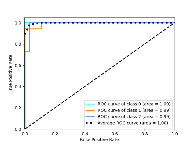
(a) Model from Scratch.

(b) PyTorch Model.

Figure 2: ROC curves of model from scratch and PyTorch model on the Iris dataset.

Implementation Time. Table IV compares the average (of 10 runs) training time (in seconds) of the model $M_{2}$ implemented from scratch (Model $M_{2}$, Plaintext, no DP), and the PyTorch baseline model (Model $M_{2}$ Baseline) on all datasets from Table II. It is observed that, training time in the plaintext of our implementation is about 100 to 300 times slower than that of the PyTorch baseline. We analysed the source code of our implementation and the PyTorch documentation and then concluded three points caused this observation.

• Due to the need to incorporate Gaussian-distributed noise, smaller negative numbers may occur, which can lead to data overflow when the activation function sigmoid is entered. Therefore our program is designed in such a way that for all model training, the sigmoid will be adjusted to Eq. (9).

  $$\text{sigmoid}(x)=\begin{cases}\frac{1}{1+e^{-x}},&\text{if}\ x\geq 0,\\ \frac{e^{x}}{1+e^{x}},&\text{otherwise.}\\ \end{cases}$$ (9)

• PyTorch optimizes low-level implementation for training, i.e., dynamic computational graphs, which means the network behaviour can be changed programmatically at training time to accelerate the training process.

• We implemented more functions to accommodate the Concrete library [16] even in the plaintext domain. A main deviation from the general neural network training is the way we treat the gradients. As discussed in Section 4.1, we calculate the gradients separately using two pathways depending on unencrypted (from $D_{1}$) vs encrypted labels (from $D_{2}$) as shown in Eq. (4). Hence, in our code, we defined a separate function for preparing a batch of sample forward propagation results, which are forced to be divided into two terms for computation.

Encrypted Domain. Zama’s current Concrete framework for TFHE [16] mandates decimals to be converted to integers. For our experiments, we chose a precision level of six decimal places, i.e., we use $r=10^{6}$. Additionally, in order to verify that the encryption operations do not affect the accuracy of our implementation, we use the Iris dataset for a simple experiment. After setting the same initialization of weights and the order of reading the datasets, we train the model from scratch in plaintext and train another model from scratch on the ciphertext, and compare the trained model parameters. The weights of the two models were almost identical up to four decimal places. The exact weights and biases are shown in Table VII in Appendix F.

Figure 3: Our homomorphic encryption circuit in Zama’s Concrete.

6.3 Protocol Implementation

We use the Concrete framework from Zama [16] to implement the TFHE components of our protocol. Note that not all the operations in our protocol require homomorphic operations. The circuit to compute the protocol operations for one sample is given in Figure 3. Given a sample $s$ of the batch $B$, from Eq. (4) in Step 4 of the protocol, we first need to multiply the derivatives of the inputs to the softmax function with the encrypted labels. Dropping subscripts and abbreviating notation, these are shown as $z_{\mathbf{w}}$ and $y$ respectively in the figure. For brevity, we skip the integer encoding step, but it is understood that $z_{\mathbf{w}}$ is multiplied by $r$ (the precision parameter), truncated, and then multiplied with $y$ as given by Eq. (4). Next, Step 6 of the protocol samples noise of scale $\mathcal{N}(0,\sigma^{2}\mathbf{1}_{R})$, which for a single entry with Gaussian differential privacy is $\eta=\mathcal{N}(0,1/\epsilon^{2})$. The noise is then multiplied by the $t$ allowable values of sensitivity and then the truncated noise value is encrypted as in Step 6 of the protocol. Again to avoid excessive notation, we simply show this as multiplying $\eta$ by one of the allowable values of sensitivity $rs$ (noting $r$ being the precision parameter). These quantiities are then added homomorphically according to Step 8 of the protocol. On the other side of the circuit, once decrypted, we get the blinded and differentially private gradients (Eq (8)), which result in the differentially private gradients after subtracting the blind.

Implementation Notes. As Concrete only accepts integer inputs, we need to convert the respective inputs to integer equivalents. To do so, we compute $z_{\mathbf{w}}$ to six decimal places, i.e., we multiply it by the precision factor $r=10^{6}$, and floor the result. Similarly, we floor $rs\cdot\eta$, since the noise is already of scale $r$. Thus, the two quantities are in effect multiples of $r=10^{6}$. Note that the label $y$ is unchanged, as it is already an integer.

6.4 Plaintext vs Ciphertext Versions of the Protocol

To ensure that the protocol replicates the scenario of Section 6.1, we evaluate our protocol against the unencrypted setting. Namely, we evaluate model $M_{1}$ on dataset $D_{1}$, model $M_{2}$ on dataset $D_{1}\cup D_{2}$, both unencrypted and without differential privacy, and model $\widetilde{M}_{2}$ on dataset $D_{1}\cup D_{2}$ computed through our protocol (with encryption and differential privacy). We use all the datasets from Table II to evaluate this. Furthermore, we retain $3,506$ features from the Drebin dataset which is a subset of all available features. The feature classes retained include ‘api_call’, ‘call’, ‘feature’, ‘intent’, ‘permission’, ‘provider’, and ‘real_permission’.

For each dataset and each value of $\epsilon$, we report the average (of 10 runs) results. Each time, the dataset is re-partitioned and $30\%$ of the data is randomly used as $D_{\text{hold}}$. Due to the different sizes of the datasets, we divide $D_{1}$ and $D_{2}$ differently for different datasets:

• For Iris, Seeds and Wine, $D_{1}$ is $10\%$ of the total data and $D_{2}$ is $60\%$ of the total data.

• For Abrupto and Drebin, $D_{1}$ is $1\%$ of the total data and $D_{2}$ is $69\%$ of the total data.

Note that we do not artificially induce a skewed distribution of samples in $D_{1}$ for these experiments, as this was done in Section 6.1.

Table IV shows the results of our experiments. The column $\epsilon$ contains the overall privacy budget. We use $t=100$ allowable values of sensitivity. In all our experiments, we found $\Delta S_{B}(\mathbf{w})$, i.e., the sensitivity of the gradients without encoding from Eq. (6), ranged from $0.019$ to $0.035$. We extended this range to $[0,0.1]$ and picked 100 evenly spaced samples as the $t=100$ allowed values of sensitivity. For datasets Iris, Seeds and Wine, training our protocol ($\widetilde{M}_{2}$) is about 10,000 times slower than training the same model in the clear ($M_{2}$). However, this time is mainly due to the encryption of the noise vector with all $t=100$ allowable values of sensitivity. The time per epoch and total time consumed in encrypting this list is shown in the column labelled “$t$-list time” in the table. The total time is obtained by multiplying per epoch time by 50, the total number of epochs. Subtracting this time means that these three datasets can be trained between 100 to 250 seconds, which is very reasonable. Note that this list of noisy sensitivities does not depend on the datasets. Therefore $P_{2}$ can precompute these lists, significantly reducing interactive time. With this speed-up our implementation is only $\approx$100 times slower than training in the clear, i.e., $M_{2}$. The $\epsilon=100$ regime gives little to no privacy. Looking at the numbers corresponding to those rows, we see that the accuracy of $\widetilde{M}_{2}$ is almost identical to $M_{2}$. This shows that our encrypted portion of the protocol does not incur much accuracy loss. For each dataset, we also show values of $\epsilon$ between $0.25$ and $0.5$, where the accuracy of $\widetilde{M}_{2}$ lies nicely in between $M_{1}$ and $M_{2}$. Thus, this value of $\epsilon$ can be used by $P_{2}$ such that $\widetilde{M}_{2}$ shows an improvement over $M_{1}$, yet at the same time, training over the noiseless data promises even more improvement.

TABLE IV: Training time and accuracy of $M_{1}$ (dataset $D_{1}$), $M_{2}$ (dataset $D_{1}\cup D_{2}$) in the clear, $\widetilde{M}_{2}$ (dataset $D_{1}\cup D_{2}$) through our protocol, $M^{\text{Py}}_{2}$ (dataset $D_{1}\cup D_{2}$) implemented in PyTorch in the clear, and ${M}^{\text{RR}}_{2}$ (dataset $D_{1}\cup D_{2}$) with randomized response (hidden neurons: 20, batch size: 256, learning rate: 0.1, epochs: 50).

Dataset	$\epsilon$	Model $M_{1}$ Plaintext, no DP		Model $M_{2}$ Plaintext, no DP		Model $\widetilde{M}_{2}$ Our protocol			Model $M^{\text{Py}}_{2}$ PyTorch baseline		Model $M^{\text{RR}}_{2}$ Randomized Response
		Time(s)	Test Acc.	Time(s)	Test Acc.	$t$-list time(s) per epoch & total	Time(s)	Test Acc.	Time(s)	Test Acc.	Test Acc.
Iris	0.1	0.0619	0.7289	0.4244	0.8467	81.3214 $\approx$4050	4162.2530	0.7733	0.0078	0.8467	0.3711
	1	0.0624	0.7289	0.4268	0.8467		4220.4972	0.8511	0.0079	0.8467	0.6244
	10	0.0616	0.7289	0.4248	0.8467		4179.3149	0.8521	0.0079	0.8467	0.8189
	100	0.0619	0.7222	0.4236	0.8444		4186.3186	0.8554	0.0079	0.8444	0.8311
	0.2	0.0618	0.7289	0.4247	0.8467		4210.8248	0.7821	0.0079	0.8467	0.3416
	0.5	0.0618	0.7289	0.4247	0.8467		4210.8248	0.8422	0.0079	0.8467	0.6266
Seeds	0.1	0.0896	0.8079	0.6216	0.8762	110.1530 $\approx$5525	5613.6482	0.6132	0.0084	0.8762	0.3682
	1	0.0889	0.8079	0.6124	0.8762		5602.3480	0.8762	0.0084	0.8762	0.6873
	10	0.0884	0.8079	0.6120	0.8762		5739.1349	0.8719	0.0083	0.8762	0.8550
	100	0.0902	0.8079	0.6219	0.8762		5689.1976	0.8730	0.0083	0.8762	0.8762
	0.2	0.0885	0.8079	0.6126	0.8762		5670.3486	0.8111	0.0083	0.8762	0.3794
	0.5	0.0897	0.8079	0.6204	0.8762		5703.6741	0.8714	0.0083	0.8762	0.6174
Wine	0.1	0.1161	0.7981	0.5265	0.9302	90.8877 $\approx$4544	4773.6742	0.7792	0.0105	0.9302	0.4361
	1	0.1046	0.7925	0.5311	0.9472		4628.6748	0.9340	0.0106	0.9472	0.7981
	10	0.0745	0.8283	0.5289	0.9483		4629.9854	0.9396	0.0089	0.9283	0.9205
	100	0.0747	0.8283	0.5313	0.9483		4665.1684	0.9396	0.0089	0.9283	0.9283
	0.2	0.0747	0.8283	0.5322	0.9283		4679.4358	0.8905	0.0081	0.9283	0.4999
	0.5	0.1155	0.8604	0.5205	0.9660		4626.1674	0.9320	0.0104	0.9660	0.5168
Abrupto	0.1	0.4212	0.8399	28.3430	0.9077	3472.1348 $\approx$173606	175797.7331	0.7794	0.2687	0.9077	0.6593
	1	0.4108	0.8331	27.8466	0.9057		175784.2495	0.9028	0.2247	0.9057	0.8869
	10	0.4065	0.8331	27.7893	0.9055		175791.6472	0.9059	0.2226	0.9055	0.9004
	100	0.4082	0.8331	28.0041	0.9067		175783.6481	0.9061	0.2238	0.9067	0.9067
	0.2	0.4214	0.8299	28.3819	0.9067		175781.3571	0.8850	0.2681	0.9067	0.7413
	0.5	0.4198	0.8331	28.4917	0.9067		175791.3479	0.9045	0.2240	0.9067	0.8916
Drebin	0.1	8.5758	0.8571	628.0991	0.9470	5760.3054 $\approx$288015	299113.0059	0.7010	2.8677	0.9470	0.6053
	1	8.4595	0.8680	635.2497	0.9507		299109.3641	0.9235	2.9562	0.9507	0.9191
	10	8.4930	0.8530	623.5984	0.9492		299124.6524	0.9462	2.9583	0.9492	0.9490
	100	8.5634	0.8871	628.6070	0.9489		299117.0157	0.9476	2.4226	0.9489	0.9489
	0.5	8.4300	0.8743	632.0590	0.9496		299111.1248	0.8860	2.5718	0.8817	0.8741
	0.7	8.6314	0.8571	638.8455	0.9470		299118.4348	0.9172	2.7122	0.9470	0.9023

The appropriate choice of $\epsilon$ depends on the size of the dataset, as it is different for the two larger datasets. One is a synthetic dataset Abrupto and the other one is a real-world Android malware dataset Drebin. Table IV also shows the results of these two larger datasets. In terms of training time, unlike small datasets, there is a significant difference in their training time. This is due to the large number of features in the Drebin dataset, which is around 876 times more than the features in the Abrupto dataset. However, once again, the majority of the time is consumed in encrypting the noisy $t$-list, which as we mentioned before, can be precomputed. Since these datasets have multiple batches per epoch, the per epoch time for the $t$-list is also higher. However, subtracting the total time of the $t$-lists, the training of these two datasets takes between 2,000 to 11,000 seconds, which is reasonably fast considering the sizes of these datasets. When $\epsilon=100$, the accuracy of $\widetilde{M}_{2}$ is almost the same or even better than that of $M_{2}$. For Abrupto datasets, at $\epsilon\in$ [0.15, 0.5] we find the spot between the accuracy of model $M_{1}$ and $M_{2}$. On the other hand, with $\epsilon\in[0.3,0.5]$ we find the spot between the accuracy of model $M_{1}$ and $M_{2}$ based on the Drebin dataset.

Randomized Response-based Protocol. In Section 4.1 we briefly mentioned that one way to obtain an updated model $M_{2}$ is for $P_{2}$ to apply differentially private noise to the labels of $D_{2}$, and then handover the noisy labelled dataset to $P_{1}$. This will then enable $P_{1}$ to run the entire neural network training in the clear, giving significant boost in training time. This can be done by adding noise to the labels via the randomized response (RR) protocol, given in [23], which is used in many previous works as well. However, our experiments show that for a reasonable guarantee of privacy of the labels, the resulting accuracy through RR is less than the accuracy of even $M_{1}$ in most cases. To be more precise, let us detail the RR protocol for binary labels. For each label, $P_{2}$ samples a bit from a Bernoulli distribution with parameter $\gamma$. If the bit is 0, $P_{2}$ keeps the true label, otherwise, $P_{2}$ replaces the label with a random binary label [23]. Note that the probability that the resulting label is the true label is $1-\gamma/2$. The mechanism is $\epsilon$-label differentially private as long as:

$$\frac{1-\gamma/2}{\gamma/2}\leq{e^{\epsilon}}\Rightarrow\epsilon\geq\ln(\gamma/2-1)$$ (10)

for all $\gamma<1$. Setting the value of $\epsilon$ exactly equal to the quantity on the right, we see that the probability that the resulting label is the true label is given by $e^{\epsilon}/(e^{\epsilon}+1)$. Thus, for instance, if $\epsilon=1$, the probability of the label being the true label is $\approx 73\%$, for $\epsilon=\ln 3$ it is $75\%$, for $\epsilon=3$ it is $\approx 95\%$, for $\epsilon=5$ it is $\approx 99.33\%$, and for $\epsilon=10$ it is $\approx 99.99\%$. Thus, for reasonable privacy we would like to choose $\epsilon$ less than 1, and definitely not close to 10, otherwise, $P_{2}$ is effectively handing over the true labels to $P_{1}$.

We trained the model by using the above mentioned RR protocol. The results are shown in Table IV under the column labelled ${M}^{\text{RR}}_{2}$. As we can see, the accuracy is less than the accuracy of even $M_{1}$ for the smaller Iris, Seeds and Wine datasets, only approaching the accuracy between $M_{1}$ and $M_{2}$ when $\epsilon$ is close to $10$, but which as we have argued above is not private enough. For the two larger datasets, Abrupto and Drebin, $\epsilon=1$ gives better accuracy than $M_{1}$ while being less than $M_{2}$. However, we achieve the same using our protocol for a significantly smaller value of $\epsilon$. This is advantageous because it means that $P_{1}$ and $P_{2}$ can do multiple collaborations without exhausting the budget.

Communication Overhead. The TLWE ciphertext is defined as $\mathbf{c}=(\mathbf{a},b)\in\mathbb{T}_{q}^{N+1}$. As mentioned in Section 2.4, we use $N=630$ and $q$ is 64 bits long. This means that the ciphertext is of size: $631\times 64=40,384$ bits. Luckily, as shown in [15], a more compact way to represent $\mathbf{c}$ is to first uniformly sample a random seed $\theta$ of 128 bits (the same level of security as the key $\mathsf{k}$), and then use a cryptographically secure PRNG to evaluate the vectors $\mathbf{a}\leftarrow\text{PRNG}(\theta)$. This ciphertext representation is only $128+64=192$ bits long (adding the bit-lengths of $\theta$ and $b$). This reduction applies only when $P_{2}$ generates fresh ciphertexts, as any homomorphic computations will, in general, not be able to keep track of the changes to the vectors $\mathbf{a}$. With these calculations, we estimate the communication cost of our protocol as follows:

• In Step 1 of the protocol, $P_{2}$ sends $m_{2}$ encrypted labels under key $\mathsf{k}$ of its dataset $D_{2}$ of size $m_{2}$. Using the compact representation just mentioned, this results in communication cost of $192m_{2}$ bits. We ignore the cost of plaintext features of $D_{2}$ being transmitted, as this cost is the same for any protocol, secure or not.

• In Step 6, $P_{2}$ sends the encryption of the $R$-element noise vector for all $t$ allowable values of sensitivity. Once again, since these are fresh encryptions under $\mathsf{k}$, we have communication cost of $192tR$ bits.

• In Step 8, $P_{1}$ sends the $R$-element encrypted, blinded and noise added vector to $P_{2}$. Since this is obtained through homomorphic operations, we use the non-compact representation, yielding $40384R$ bits of communication cost.

• Lastly, in Step 9 $P_{2}$ sends the decrypted version of the quantity above. The communication cost is less than $64R$ bits, as this is plaintext space.

Note that Step 6, 8 and 9 need to be repeated for every batch in an epoch. Let $m_{1,2}$ be the size of the dataset $D_{1}\cup D_{2}$. Then the number of times these steps are repeated in each epoch is given by $\lceil m_{1,2}/|B|\rceil$, where $|B|$ is the batch size. Thus the total communication cost for one epoch is $192m_{2}+(192tR+40384R+64R)(\lceil m_{1,2}/|B|\rceil=192m_{2}+(192tR+40448R)(\lceil m_{1,2}/|B|\rceil$. Over $n$ epochs, the communication cost in bits is thus:

$$C=\left(192m_{2}+\left(192t+40448\right)R\left\lceil\frac{m_{1,2}}{|B|}\right\rceil\right)n$$ (11)

For the datasets in Table IV, we have $R=40$, since the number of hidden neurons is 20 (and binary classification), number of epochs $n=50$, and $t=100$. The size of $D_{2}$, i.e., $m_{2}$ is $0.6m$ for Iris, Seeds and Wine datasets, and equals $0.69m$ for the remaining two datasets where $m$ is the total size of the datasets as mentioned in Section 6.4. For all datasets we have $m_{1,2}=0.7m$. The batch size $|B|=256$. The communication cost in units of megabytes MB is shown in Table V. By far, the major cost is the $t$ encrypted noise values which need to be sent for each batch in an epoch in case of larger datasets. As mentioned earlier, these encrypted noise vectors can be generated well in advance to reduce interactive communication cost, as they do not use of any data specific parameter. For instance, with precomputed noise lists, the communication cost on the Drebin dataset reduces to 9.54MB per epoch. These times without the encrypted noise vectors are shown in the last two columns of the table labelled “no $t$-list.” Regardless, we see that communication in each round of the protocol (each epoch) can be done in a few seconds with typical broadband speeds.

TABLE V: Communication cost in megabytes (MBs) of our protocol as calculated through Eq. 11 for the five datasets used in our implementation.

Dataset	Size	Cost per epoch	Total cost	Cost per epoch	Total cost
	$m$			no $t$-list	no $t$-list
Iris	150	1.16MB	58.22MB	0.20MB	10.22MB
Seeds	210	1.17MB	58.26MB	0.21MB	10.26MB
Wine	178	1.16MB	58.24MB	0.20MB	10.24MB
Abrupto	10,000	32.69MB	1,634.34MB	5.81MB	290.33MB
Drebin	16,680	53.70MB	2,685.16MB	9.54MB	477.16MB

6.5 Discussion – Privacy Budget, Training Time and Limitations

Setting $\epsilon$ for Data Collaboration. The value of $\epsilon$ used depends on the size of the dataset, with a smaller $\epsilon$ required for larger datasets. However, for all the datasets used in the experiment, with $\epsilon$ in the range $(0.3,0.5)$ the accuracy of the model $\widetilde{M_{2}}$ is higher than that of $M_{1}$, and lower than that of $M_{2}$. Thus, party $P_{2}$ can set an $\epsilon$ within this range, which provides visible benefits for $P_{1}$ to proceed with data collaboration in the clear.

Fast Training of Our Protocol. The training time of our protocol (Table IV) is many orders of magnitude faster than protocols using entirely FHE operation reported in [2, 3, 5]. This is a direct result of keeping the forward and backward propagation in the clear even though some labels from the training data are encrypted. To compare the training time of our protocol against an end-to-end encrypted solution for neural network training, we look at the work from [2]. They use polynomial approximations for the activation functions (e.g., sigmoid) to allow homomorphic operations. In one set of experiments, they train a neural network with one hidden layer over the Crab dataset, which has 200 rows and two classes. This dataset is comparable in size and number of classes to the Iris dataset used by us. They implement the homomorphically encrypted training of the neural network using HELib [24]. The time required for training one batch per epoch is 217 seconds (Table 3a in [2]). For 50 epochs, and processing all batches in parallel, this amounts to 10,850 seconds. We note that after each round the ciphertext is sent to the client to re-encrypt and send fresh ciphertexts back to the server in order to reduce noise due to homomorphic operations. Thus, this time is a crude lower bound on the total time. In comparison, our protocol takes a total time of around 4,200 seconds for the entire 50 epochs over the comparable Iris dataset with one hidden layer, and just 150 seconds if the noise lists are pre-processed. (Table  IV). With a more optimised implementation (say via PyTorch), this time can be reduced even further.

Implementation Limitations. The minimum value of the total budget $\epsilon$ tested by us is $0.1$. This is because of the limitation of Concrete in handling high precision real numbers (as they need to be converted into integers). When we inject differentially private noise using a (very) small $\epsilon$, it is highly likely to be inaccurate as it generate numbers with large absolute value, leading to the float overflow problem for sigmoid. In addition to that, our implementation of a neural network is many orders of magnitude slower than the PyTorch benchmark even though our accuracy matches that of the PyTorch baseline. If we are able to access gradients in a batch from the PyTorch implementation, then we would significantly accelerate the proposed protocol. For instance, the model $\widetilde{M}_{2}$ through our protocol takes 5-6 times more than $M_{2}$ (via our implementation) on the Drebin dataset (see Table IV). This means that we can potentially run our protocol between 14 to 18 seconds if the protocol is run over PyTorch’s implementation.

7 Related Work

The closest work to ours is that of Yuan et al [17]. They assume a scenario where one of the two parties holds the feature vectors and the labels are secret shared between the two parties. The goal is to jointly train a neural network on this dataset. At the end of the protocol, the first party learns the trained model whereas the second party does not learn anything. Like us, they use label differential privacy to obtain a more computationally efficient solution. Our scenario is different in that it enables party $P_{1}$ to assess the quality of the resulting dataset without knowing the model, where $P_{1}$ does not initially trust the labelling from $P_{2}$. Another major difference is that we use FHE instead of secure multiparty computation (SMC) to train the model [17]. Moreover, it is unclear whether their protocol remains differentially private as they also encode the noise in the group of integers modulo a prime before multiplying with encoded sensitivity. As mentioned in Section 4.2, this multiplication no longer means that the resulting Gaussian is appropriately scaled, resulting in violation of differential privacy. Another difference is that they share the gradient after each epoch between the two parties, which we hide from $P_{2}$.

Apart from Yuan et al [17], several works have investigated training neural network models entirely in the encrypted domain, encompassing both features and labels [2, 3, 4, 5, 6]. Hesamifard et al [2] propose the CryptoDL framework, which employs Somewhat Homomorphic Encryption (SWHE) and Leveled Homomorphic Encryption (LHE) on approximated activation functions to facilitate interactive deep neural network training over encrypted training sets. However, the training time is prolonged even on small datasets (e.g., on the Crab dataset with dimensions of $200\times 6$ cells, it takes over $200$ seconds per epoch/iteration during the training phase). Furthermore, the omission of details regarding the CPU clock speed (frequency) and the number of hidden layer neurons in their experiments renders the reported training time less equitable. Nandakumar et al [3] introduce the first fully homomorphic encryption (FHE)-based stochastic gradient descent technique (FHE-SGD). As pioneers in this field, FHE-SGD investigates the feasibility of training a DNN in the fixed-point domain. Nevertheless, it encounters substantial training time challenges due to the utilisation of BGV-lookup-table-based sigmoid activation functions. Lou et al [5] present the Glyph framework, which expedites training for deep neural networks by alternation between TFHE (Fast Fully Homomorphic Encryption over the Torus) and BGV [25] cryptosystems. However, Glyph heavily relies on transfer learning to curtail the required training epochs/iterations, significantly reducing the overall training time for neural networks. It should be noted that Glyph’s applicability is limited in scenarios where a pre-trained teacher model is unavailable. Xu et al propose CryptoNN [4], which employs functional encryption for inner-product [26] to achieve secure matrix computation. However, the realisation of secure computation in CryptoNN necessitates the presence of a trusted authority for the generation and distribution of both public and private keys, a dependency that potentially compromises the security of the approach. NN-emd [6] extends CryptoNN’s capabilities to support training a secure DNN over vertically partitioned data distributed across multiple users.

By far, the major bottleneck of end-to-end homomorphic encryption or functional encryption approaches to neural network training is the run-time. For instance, a single mini-batch of 60 samples can take anywhere from 30 seconds to several days with dedicated memory [6]. Another option is to use a secure multiparty computation (SMC) approach. In this case, the (joint) dataset can be secret shared between two parties, and they can jointly train the model learning only the trained model [27]. However, once again end-to-end SMC solutions remain costly. For instance, the work from  [27] achieves SMC-based neural network training in 21,000 seconds with a network of 3 layers and 266 neurons. Undoubtedly, these benchmarks are being surpassed, e.g., [28], however, it is unlikely that they will achieve the speed achieved by our solution, or the one from Yuan et al. [17].

A related line of work looks at techniques to check the validity of inputs without revealing them. For instance, one can use zero-knowledge range proofs [29] to check if an input is within an allowable range without revealing the input, e.g., age. This has, for instance, been used in privacy-preserving joint data analysis schemes such as Drynx [30] and Prio [31] to ensure that attribute values of datasets are within the allowable range. However, in our case, we do not assume that the party $P_{2}$ submits any label that is out of range. Instead, the party may not have the domain expertise to label feature vectors correctly. This cannot be determined through input validity checking.

8 Conclusion

We have shown how two parties can assess the value of their potential machine learning collaboration without revealing their models and respective datasets. With the use of label differential privacy and fully homomorphic encryption over the torus, we are able to construct a protocol for this use case which is many orders of magnitude more efficient than an end-to-end homomorphic encryption solution. Our work can be improved in a number of ways. One direction is to go beyond the honest-but-curious model and assume malicious parties. A key challenge is to maintain efficiency as several constructs used by us cannot be used in the malicious setting, e.g., the use of the random blind. Due to several limitations in accessing components in PyTorch’s neural network implementation and the integer input requirement in Zama’s Concrete TFHE framework, our implementation is short of speedups that can potentially be achieved. As a result, we are also not able to test our protocol on larger datasets (say, 100k or more rows). Future versions of this framework may remove these drawbacks. Finally, there could be other ways in which two parties can check the quality of their datasets. We have opted for the improvement in the model as a proxy for determining the quality of the combined dataset.

Appendix A Proofs of Theorems from Section 3

Proof of Theorem 1

Proof.

Consider $(x,y)\sim D_{\text{hold}}$. We consider the probability:

$$\Pr[M(x)\neq y],$$

where the probability is over the coin tosses of the learning algorithm $\mathcal{A}$ that outputs $M$, and the distribution of samples in $D_{\text{hold}}$. Since we sample points from $D_{\text{hold}}$ uniformly at random, the above probability is exactly ${L}_{\text{hold}}(M)$. We have

$$\Pr[M(x)\neq y] =\Pr[M(x)\neq y\mid y=1]\Pr[y=1]$$

$$+\Pr[M(x)\neq y\mid y=0]\Pr[y=0]$$

$$=\Pr[M(x)=0\mid y=1]\Pr[y=1]$$

$$+\Pr[M(x)=1\mid y=0]\Pr[y=0]$$

Now, the learning algorithm $\mathcal{A}$’s input, i.e., $D$, remains unchanged whether $y$, i.e., the label of $x$ in $D_{\text{hold}}$, is equal to 0 and 1. This is because $D$ is labelled by $g$ which is independent of the true label $y$ (Eq. 2). Therefore,

$$\Pr[M(x)=0\mid y=1]=\Pr[M(x)=0],$$

and

$$\Pr[M(x)=1\mid y=0]=\Pr[M(x)=1].$$

We get:

$$\Pr[M(x)\neq y] =\Pr[M(x)=0]\Pr[y=1]$$

$$+\Pr[M(x)=1]\Pr[y=0]$$

$$=\Pr[M(x)=0]\frac{1}{2}+\Pr[M(x)=1]\frac{1}{2}$$

$$=\frac{1}{2}(\Pr[M(x)=0]+\Pr[M(x)=1])=\frac{1}{2}$$

Therefore ${L}_{\text{hold}}(M)=\Pr[M(x)\neq y]=\frac{1}{2}$. ∎

Proof of Theorem 2

Proof.

Since $D_{2}$ is labelled according to $g$, it does not increase $\mathcal{A}$’s information about $D_{\text{hold}}$. Therefore, the overall error of $M_{2}$ on $D_{\text{hold}}$ can at best be greater than or equal to that of $M_{1}$ on $D_{\text{hold}}$, as both are outputs of the same learning algorithm $\mathcal{A}$. In other words, if $(x,y)\sim D_{\text{hold}}$ then

$$\Pr[M_{2}(x)=0\mid y=1]+\Pr[M_{2}(x)=1\mid y=0]$$

$$\geq\Pr[M_{1}(x)=0\mid y=1]+\Pr[M_{1}(x)=1\mid y=0],$$

where once again the probabilities are also over the coin tosses of the algorithm $\mathcal{A}$ generating $M_{1}$ and $M_{2}$. Notice that this does not necessarily mean, for instance, that $\Pr[M_{2}(x)=0\mid y=1]\geq\Pr[M_{1}(x)=0\mid y=1]$, since $M_{2}$ may assign the label 1 to every sample. Now since $D_{\text{hold}}$ is balanced, for $(x,y)\sim D_{\text{hold}}$, we have

$$\Pr[M_{2}(x)\neq y] =\Pr[M_{2}(x)=0\mid y=1]\Pr[y=1]$$

$$+\Pr[M_{2}(x)=1\mid y=0]\Pr[y=0]$$

$$=\frac{1}{2}(\Pr[M_{2}(x)=0\mid y=1]$$

$$+\Pr[M_{2}(x)=1\mid y=0])$$

$$\geq\frac{1}{2}(\Pr[M_{1}(x)=0\mid y=1]$$

$$+\Pr[M_{1}(x)=1\mid y=0])$$

$$=\Pr[M_{1}(x)\neq y].$$

Therefore, ${L}_{\text{hold}}(M_{2})\geq{L}_{\text{hold}}(M_{1})$. ∎

Appendix B Computing Gradients via the Chain Rule

From Equation (3), we are interested in computing the loss through the samples in a batch $B$ that belong to the dataset $D_{2}$. Overloading notation, we still use $B$ to denote the samples belonging to $D_{2}$. The algorithm used to minimizing the loss is the stochastic gradient descent algorithm using backpropagation. This inolves calculating the gradient $\nabla L_{B}(\mathbf{w})$. As noted in [17], if we are using the backpropagation algorithm, we only need to be concerned about the gradients corresponding to the last layer. Again, to simplify notation, we denote the vector of weights in the last layer by $\mathbf{w}$.

Let $s=(\mathbf{x},\mathbf{y})$ be a sample in the batch $B$. Let $K$ denote the number of classes. We assume that $\mathbf{y}$ is one-hot encoded, meaning that only one of its element is 1, and the rest are zero. We denote the index of this element by $c$ (which of course is different for different samples). The output from the neural network is the softmax output $\mathbf{p}$ of size $K$, where:

$$p_{i}=\frac{e^{z_{i}}}{\sum_{j}e^{z_{j}}},$$

where $\mathbf{z}=(z_{1},\ldots,z_{K})$ is the output before the softmax layer. Consider the cross-entropy loss. Under this loss, we have:

$$L_{s}(\mathbf{w})=-\sum_{i=1}^{K}y_{i}\ln p_{i}=-\ln p_{c},$$ (12)

since $\mathbf{y}$ is one-hot encoded. Now, we have:

$$\nabla L_{B}(\mathbf{w})=\frac{1}{|B|}\sum_{s\in B}\nabla L_{s}(\mathbf{w})$$ (13)

Let us, therefore, focus on the gradient of per-sample loss. By the chain rule, we have:

$$\nabla L_{s}(\mathbf{w})=\frac{\partial L}{\partial\mathbf{w}}=\frac{\partial L}{\partial\mathbf{z}}\frac{\partial\mathbf{z}}{\partial\mathbf{w}}$$ (14)

Consider the $i$th element of $\frac{\partial L}{\partial\mathbf{z}}$:

$$\frac{\partial L}{\partial z_{i}} =\frac{\partial}{\partial z_{i}}\left(-\ln p_{c}\right)=-\frac{1}{p_{c}}\frac{\partial p_{c}}{\partial z_{i}}.$$ (15)

Solving for the case when $i=c$, the above becomes $p_{c}-1$, whereas for the case $i\neq c$, we get $p_{i}$. In both cases, we get:

$$\frac{\partial L}{\partial z_{i}}=p_{i}-\mathbf{1}_{c}(i)=p_{i}-y_{i}$$

Plugging this into Equation (14), we get:

$$\nabla L_{s}(\mathbf{w})=\sum_{i=1}^{K}(p_{i}-\mathbf{1}_{c}(i))\frac{\partial z_{i}}{\partial\mathbf{w}}$$ (16)

Plugging this into Equation (13), we get:

$$\nabla L_{B}(\mathbf{w}) =\frac{1}{|B|}\sum_{s\in B}\sum_{i=1}^{K}(p_{i}(s)-\mathbf{1}_{c(s)}(i))\frac{\partial z_{i}(s)}{\partial\mathbf{w}}$$

$$=\frac{1}{|B|}\sum_{s\in B}\sum_{i=1}^{K}p_{i}(s)\frac{\partial z_{i}(s)}{\partial\mathbf{w}}$$

$$-\frac{1}{|B|}\sum_{s\in B}\sum_{i=1}^{K}\mathbf{1}_{c(s)}(i)\frac{\partial z_{i}(s)}{\partial\mathbf{w}},$$ (17)

where $c(s),p_{i}(s)$ and $z_{i}(s)$ denote the fact that these quantities depend on the sample $s$.

Appendix C Sensitivity of the Gradient of the Loss Function

We now compute the $\ell_{2}$-sensitivity of the loss function. Let $D^{\prime}$ and $D^{\prime\prime}$ be neighbouring datasets, where all but one of the samples have the labels changed to another label. Let $s^{\prime}$ and $s^{\prime\prime}$ represent the differing samples. Let $B^{\prime}$ and $B^{\prime\prime}$ be the batches drawn in the two datasets. Note that $|B^{\prime}|=|B^{\prime\prime}|$ and we denote this by $|B|$. Then, the $\ell_{2}$-sensitivity of the loss function, when no encoding is employed, is:

$$\lVert\nabla L_{B^{\prime}}(\mathbf{w})-\nabla L_{B^{\prime\prime}}(\mathbf{w})\rVert_{2}$$

$$=\frac{1}{|B|}\left\lVert\sum_{s\in B^{\prime}}\nabla L_{s}(\mathbf{w})-\sum_{s\in B^{\prime\prime}}\nabla L_{s}(\mathbf{w})\right\rVert_{2}$$

$$=\frac{1}{|B|}\left\lVert\nabla L_{s^{\prime}}(\mathbf{w})-\nabla L_{s^{\prime\prime}}(\mathbf{w})\right\rVert_{2}$$

$$=\frac{1}{|B|}\left\lVert\sum_{i=1}^{K}(p_{i}-\mathbf{1}_{c(s^{\prime})}(i))\frac{\partial z_{i}}{\partial\mathbf{w}}\right.$$

$$-\left.\sum_{i=1}^{K}(p_{i}-\mathbf{1}_{c(s^{\prime\prime})}(i))\frac{\partial z_{i}}{\partial\mathbf{w}}\right\rVert_{2}$$

$$=\frac{1}{|B|}\left\lVert\sum_{i=1}^{K}(\mathbf{1}_{c(s^{\prime\prime})}(i)-\mathbf{1}_{c(s^{\prime})}(i))\frac{\partial z_{i}}{\partial\mathbf{w}}\right\rVert_{2}$$

$$\leq\frac{1}{|B|}\sum_{i=1}^{K}\left\lVert(\mathbf{1}_{c(s^{\prime\prime})}(i)-\mathbf{1}_{c(s^{\prime})}(i))\frac{\partial z_{i}}{\partial\mathbf{w}}\right\rVert_{2}$$

$$=\frac{1}{|B|}\sum_{i=1}^{K}\left\lvert\mathbf{1}_{c(s^{\prime\prime})}(i)-\mathbf{1}_{c(s^{\prime})}(i)\right\rvert\left\lVert\frac{\partial z_{i}}{\partial\mathbf{w}}\right\rVert_{2}$$

$$\leq\frac{1}{|B|}\left(\sum_{i=1}^{K}\left\lvert\mathbf{1}_{c(s^{\prime\prime})}(i)-\mathbf{1}_{c(s^{\prime})}(i)\right\rvert\right)\max_{i}\left\lVert\frac{\partial z_{i}}{\partial\mathbf{w}}\right\rVert_{2}$$

$$=\frac{2}{|B|}\max_{i}\left\lVert\frac{\partial z_{i}}{\partial\mathbf{w}}\right\rVert_{2}$$

And over all possible choice of samples $s$ in the batch, we get that

$$\lVert\nabla L_{B^{\prime}}(\mathbf{w})-\nabla L_{B^{\prime\prime}}(\mathbf{w})\rVert_{2} \leq\frac{2}{|B|}\max_{i,s}\left\lVert\frac{\partial z_{i}(s)}{\partial\mathbf{w}}\right\rVert_{2}$$

$$=\Delta S_{B}(\mathbf{w}),$$ (18)

where $z_{i}(s)$ is the $i$th coordinate of the vector $\mathbf{z}$ in the sample $s$.

Now, in Step 4 of our protocol the partial derivative vector $\frac{\partial z_{i}(s)}{\partial\mathbf{w}}$ from Eq. 17 is encoded as:

$$\left\lfloor r\frac{\partial z_{i}(s)}{\partial\mathbf{w}}\right\rfloor.$$

Plugging this instead of the partial derivative vector in Eq. 17, we see that the expression remains the same except that now the partial derivative vector has been changed. Therefore, from Eq. 18, we get:

$$\lVert\nabla\widetilde{L}_{B^{\prime}}(\mathbf{w})-\nabla\widetilde{L}_{B^{\prime\prime}}(\mathbf{w})\rVert_{2}\leq\frac{2}{|B|}\max_{i,s}\left\lVert\left\lfloor r\frac{\partial z_{i}(s)}{\partial\mathbf{w}}\right\rfloor\right\rVert_{2},$$

where $\widetilde{L}$ represents the loss function using the encoded partial derivative vector. Next we use the following proposition:

Proposition 4.

Let $\mathbf{x}\in\mathbb{R}^{m}$ and $r$ be a positive integer. Then

$$\lVert\lfloor r\mathbf{x}\rfloor\rVert_{2}\leq r\lVert\mathbf{x}\rVert_{2}.$$

Proof.

We have

$$\lVert\lfloor r\mathbf{x}\rfloor\rVert_{2} =\sqrt{\sum_{i=1}^{m}(\lfloor rx_{i}\rfloor)^{2}}$$

$$\leq\sqrt{\sum_{i=1}^{m}(rx_{i})^{2}}=r\sqrt{\sum_{i=1}^{m}(x_{i})^{2}}=r\lVert\mathbf{x}\rVert_{2}.$$

∎

Let us denote the vector $\frac{\partial z_{i}(s)}{\partial\mathbf{w}}$ which maximizes $\left\lVert\left\lfloor r\frac{\partial z_{i}(s)}{\partial\mathbf{w}}\right\rfloor\right\rVert_{2}$ as $\mathbf{z}$. Then, in light of the above proposition and Eq. 18:

$$\lVert\nabla\widetilde{L}_{B^{\prime}}(\mathbf{w})-\nabla\widetilde{L}_{B^{\prime\prime}}(\mathbf{w})\rVert_{2} \leq\frac{2}{|B|}\max_{i,s}\left\lVert\left\lfloor r\frac{\partial z_{i}(s)}{\partial\mathbf{w}}\right\rfloor\right\rVert_{2}$$

$$=\frac{2}{|B|}\left\lVert\left\lfloor r\mathbf{z}\right\rfloor\right\rVert_{2}$$

$$\leq\frac{2}{|B|}r\left\lVert\mathbf{z}\right\rVert_{2}$$

$$\leq\frac{2}{|B|}r\max_{i,s}\left\lVert\frac{\partial z_{i}(s)}{\partial\mathbf{w}}\right\rVert_{2}$$

$$=r\Delta S_{B}(\mathbf{w})$$ (19)

Appendix D Proving Security

We will prove security in the universal composability framework [18, §23.5],[19]. Under this framework, we need to consider how we can define ideal functionality for $P_{2}$. More specifically, $P_{2}$ applies differentially private (DP) noise at places in the protocol. One way around this is to assume that the ideal functionality applies DP noise to the labels of $P_{2}$’s dataset at the start, and uses these noisy labels to train the dataset. However, this may cause issues with the amount of DP noise added in the ideal world vs the real world. To get around this, we assume that the ideal functionality does the same as what happens in the real-world, i.e., in each batch, the ideal functionality adds noise according to the sensitivity of the batch. We can then argue that the random variables representing the output in both settings will be similarly distributed. We assume $R$, the number of weights in the last layer, $|B|$, the batch size, and the number of epochs to be publicly known.

The ideal world. In the ideal setting, the simulator $\mathcal{S}$ replaces the real-world adversary $\mathcal{B}$. The ideal functionality $\mathcal{F}$ for our problem is defined as follows. The environment $\mathcal{Z}$ hands to $\mathcal{F}$ inputs $D_{1}$, hold-out set $D_{\text{hold}}$, learning algorithm $\mathcal{A}$, $L_{\text{hold}}({M_{1}})$, where $M_{1}\leftarrow\mathcal{A}(D_{1})$, and the features of the dataset $D_{2}$, i.e., without the labels, which is the input to party $P_{1}$. The environment $\mathcal{Z}$ also gives dataset $D_{2}$ to $\mathcal{F}$ which is the input to party $P_{2}$. Finally, the environment gives the parameters $R$ (number of weights in the last layer), batch size $|B|$, number of epochs $n$, precision parameter $r$, the privacy parameter $\epsilon$, and the list of $t$ allowable sensitivities to the ideal functionality $\mathcal{F}$. The ideal functionality sets $D\leftarrow D_{1}\cup D_{2}$. Then for each epoch, it samples a random batch $B$ of size $|B|$ from $D$. If there is at least one element in $B$ from $D_{2}$, it computes the sensitivity of the gradients of the loss function for the current batch. It then looks up the smallest value $s$ in the list of allowable sensitivity values which is greater than or equal to the computed sensitivity, and generates DP-noise $rs\mathcal{N}(0,\sigma^{2}\mathbf{1}_{R})$, and adds it to the quantity $N_{B}(\mathbf{w})$ as $N_{B}(\mathbf{w})+\lfloor rs\mathcal{N}(0,\sigma^{2}\mathbf{1}_{R})\rfloor=\widetilde{N}_{B}(\mathbf{w})$. $\mathcal{F}$ then sends the current batch $B$ and the quantity $\widetilde{N}_{B}(\mathbf{w})$ to $P_{1}$. $\mathcal{F}$ then decodes the quantity as $\widetilde{N}_{B}(\mathbf{w})/r$ and continues with backpropogation. Note that if $B$ does not contain any sample from $D_{2}$, the quantity $\widetilde{N}_{B}(\mathbf{w})$ is not sent. At the end, the functionality outputs 1 if $L_{\text{hold}}(M_{2})<L_{\text{hold}}(M_{1})$, where $M_{2}$ is the resulting training model on dataset $D$ using algorithm $\mathcal{A}$. Each party’s input is forwarded directly to the ideal functionality $\mathcal{F}$. $\mathcal{S}$ may ask the ideal functionality for the inputs to and outputs from a corrupt party. Since we assume the honest-but-curious model, $\mathcal{S}$ cannot modify these values.

The real world. In the real world, the environment $\mathcal{Z}$ supplies the inputs (both private and public) to and receives the outputs from both parties. Any corrupt party immediately reports any message it receives or any random coins it generates to the environment $\mathcal{Z}$.

Simulation when $P_{1}$ is corrupt. $\mathcal{S}$ first obtains the inputs to $P_{1}$ directly from the ideal functionality.

• At some point $\mathcal{Z}$ will generate a control message which results in the real-world $P_{1}$ receiving the encrypted dataset $D_{2}$ from real-world $P_{2}$ (Step 1). To simulate this, $\mathcal{S}$ generates $|D_{2}|$ fresh samples from the distribution $\mathcal{D}_{0}$ from Definition 3, and adds one to each row of $D_{2}$ as the purported encrypted label. $\mathcal{S}$ reports this encrypted dataset to $\mathcal{Z}$, just like real-world $P_{1}$ would do. After this step the two encrypted databases (real and simulated) are statistically indistinguishable due to the TLWE assumption over the torus (Definition 3).

• At a later point $\mathcal{Z}$ generates a control message resulting in $P_{1}$ receiving $t$ encrypted $R$-element noise vectors (one for each allowable value of sensitivity) from $P_{2}$ (Step 6). To simulate this, $\mathcal{S}$ again generates $tR$ fresh samples from $\mathcal{D}_{0}$, and reports the $t$ encrypted $R$-element vectors as the supposed noise vectors to $\mathcal{Z}$. Notice that, the length of each vector does not depend on the number of elements in the batch belonging to $D_{2}$, as long as there is at least one. If none are from $D_{2}$, then $P_{1}$ will not ask $P_{2}$ to send a noise vector. Once again, at this step the real and simulated outputs are statistically indistinguishable under the TLWE assumption over the torus.

• Lastly, $\mathcal{Z}$ generates a control message resulting in $P_{1}$ obtaining the blinded and noise-added $R$-element vector $N_{B}(\mathbf{w})$ (Step 9). $\mathcal{S}$ queries $\mathcal{F}$ to obtain the batch $B$ and the quantity $\widetilde{N}_{B}(\mathbf{w})$. If the batch $B$ does not contain any sample from $D_{2}$, $\mathcal{S}$ does nothing. Otherwise, it generates a blind vector $\boldsymbol{\mu}$ (Step 8 of the protocol), by generating fresh coins to generate $R$ elements uniformly at random from $\mathcal{P}$. $\mathcal{S}$ reports these coins to $\mathcal{Z}$. $\mathcal{S}$ reports $\widetilde{N}_{B}(\mathbf{w})+\boldsymbol{\mu}$ to $\mathcal{Z}$. At this step the real and simulated outputs are perfectly indistinguishable. due to the fact that the blinds are generated uniformly at random.

• If this is the last epoch, $\mathcal{S}$ sends the output returned by $\mathcal{F}$ to $P_{1}$ dutifully to $\mathcal{Z}$.

Thus, overall the output of the environment is statistically indistinguishable from the ideal case under the TLWE assumption over the torus.

Simulation when $P_{2}$ is corrupt. The simulation from $\mathcal{S}$ is as follows.

• When $\mathcal{Z}$ sends the initial input to $P_{2}$, $\mathcal{S}$ queries $\mathcal{F}$ to obtain this input. At the same time, $\mathcal{S}$ generates fresh coins and uses them to generate the key $\mathsf{k}$ for the TLWE scheme. $\mathcal{S}$ reports these coins to $\mathcal{Z}$.

• For generation of Gaussian noise, $\mathcal{S}$ generates an $R$-element noise vector using fresh coins as $\mathcal{N}(0,\sigma^{2}\mathbf{1}_{R})$. Then for each $s$ in the list of allowable sensitivities, $\mathcal{S}$ computes $rs\mathcal{N}(0,\sigma^{2}\mathbf{1}_{R})$. $\mathcal{S}$ then encrypts each of these $t$ vectors under $\mathsf{k}$ as $\left\llbracket\lfloor rs\mathcal{N}(0,\sigma^{2}\mathbf{1}_{R})\rfloor\right\rrbracket_{\mathsf{k}}$. $\mathcal{S}$ reports these coins to the environment $\mathcal{Z}$ (as the real-world $P_{2}$ would do).

• At some point $\mathcal{Z}$ generates a control message resulting in $P_{2}$ receiving the encrypted, blinded and noise-added $R$-element vector $N_{B}(\mathbf{w})$ (Step 8). $\mathcal{S}$ generates $R$ elements uniformly at random from $\mathcal{P}$, and then encrypts the resulting $R$-element vector under $\mathsf{k}$. $\mathcal{S}$ hands this to $\mathcal{Z}$ as the purported received vector.

• If this is the last epoch, $\mathcal{S}$ sends the output returned by $\mathcal{F}$ to $P_{2}$ dutifully to $\mathcal{Z}$.

In this case, in each step, the simulation is perfect. We are using the fact that the blinds used completely hide the underlying plaintext.

Appendix E Neural Network Weights of PyTorch vs Our Implementation

Table VI below shows the weights and biases of the neural network trained via our implementation from scratch versus the PyTorch implementation.

TABLE VI: Weights and biases of of the neural network training from scratch versus neural netowrk from PyTorch (hidden neurons: [4,4], batch size: 16, learning rate: 0.1, epochs: 100).

Input layer to hidden layer 1
Type	Weights				Bias
Ours	$-0.4916$	$-$0.6516	1.0534	0.6013	$-$0.2006
	0.298	0.4451	$-$0.7782	$-$0.2451	0.119
	$-$0.4741	$-$0.7003	1.1115	0.4583	$-$0.2123
	0.3005	0.6029	$-$0.754	$-$0.6411	0.1407
PyTorch	$-$0.4916	$-$0.6516	1.0534	0.6013	$-$0.2006
	0.2980	0.4451	$-$0.7782	$-$0.2451	0.119
	$-$0.4741	$-$0.7003	1.1115	0.4583	$-$0.2123
	0.3005	0.6029	$-$0.754	$-$0.6411	0.1407
Hidden layer 1 to hidden layer 2
Type	Weights				Bias
Ours	$-$1.4098	0.94	$-$1.3221	1.0272	0.4485
	1.1843	$-$0.5146	1.0718	$-$0.9094	$-$0.2474
	$-$0.8463	0.5649	$-$1.0814	0.7063	0.2926
	1.0468	$-$0.4571	1.0761	$-$0.6371	$-$0.1646
PyTorch	$-$1.4098	0.94	$-$1.3221	1.0272	0.4485
	1.1843	$-$0.5146	1.0718	$-$0.9094	$-$0.2474
	$-$0.8463	0.5649	$-$1.0814	0.7063	0.2926
	1.0468	$-$0.4571	1.0761	$-$0.6371	$-$0.1646
Hidden layer 2 to output layer
Type	Weights				Bias
Ours	2.0928	$-$1.7484	1.3045	$-$1.6554	-
	$-$0.1631	0.3837	0.1516	0.4605	-
	$-$2.1381	1.5229	$-$1.2348	1.0557	-
PyTorch	2.0928	$-$1.7484	1.3045	$-$1.6554	-
	$-$0.1631	0.3837	0.1516	0.4605	-
	$-$2.1381	1.5229	$-$1.2348	1.0557	-

Appendix F Neural Network Weights of Our Model in Plaintext vs Ciphertext

Table VII shows the weights and biases of our neural network model when no encryption is involved (plaintext) versus those of the model implemented through Zama’s Concrete, i.e., with homomorphic opertions.

TABLE VII: Weights and biases of models trained on the Iris dataset in plaintext and ciphertext (hidden neurons: 4, batch size: 16, learning rate: 0.1, epochs: 50).

Input layer to hidden layer 1
Type	Weight				Bias
Model Trained on Plaintext	0.6511	0.0704	0.2909	1.0547	$-0.3171$
	0.4029	$-0.4721$	1.2437	0.6597	0.472
	$-0.374$	0.5	$-0.9141$	$-0.512$	0.0603
	$-0.3569$	0.3907	$-0.9173$	$-0.8551$	$-0.0134$
Model Trained on Ciphertext	0.6511	0.0704	0.2909	1.0546	$-0.3171$
	0.4029	$-0.4721$	1.2437	0.6597	0.472
	$-0.374$	0.4999	$-0.9141$	$-0.5119$	0.0603
	$-0.3569$	0.3907	$-0.9173$	$-0.8551$	$-0.0135$
Hidden layer 1 to output layer
Type	Weight				Bias
Model Trained on Plaintext	$-1.0483$	$-1.8553$	1.194	1.3057	-
	$-0.4617$	0.8366	0.2772	$-0.0569$	-
	0.9567	0.822	$-0.9533$	$-1.4343$	-
Model Trained on Ciphertext	$-1.0483$	$-1.8553$	1.194	1.3057	-
	$-0.4617$	0.8366	0.2772	$-0.0569$	-
	0.9566	0.822	$-0.9533$	$-1.4343$	-

References

- [1] G. Widmer and M. Kubat, “Learning in the presence of concept drift and hidden contexts,” Machine learning, vol. 23, pp. 69–101, 1996.
- [2] E. Hesamifard, H. Takabi, M. Ghasemi, and R. N. Wright, “Privacy-preserving machine learning as a service.” Proc. Priv. Enhancing Technol., vol. 2018, no. 3, pp. 123–142, 2018.
- [3] K. Nandakumar, N. Ratha, S. Pankanti, and S. Halevi, “Towards deep neural network training on encrypted data,” in Proceedings of the IEEE/CVF Conference on Computer Vision and Pattern Recognition Workshops, 2019, pp. 0–0.
- [4] R. Xu, J. B. Joshi, and C. Li, “Cryptonn: Training neural networks over encrypted data,” in 2019 IEEE 39th International Conference on Distributed Computing Systems (ICDCS). IEEE, 2019, pp. 1199–1209.
- [5] Q. Lou, B. Feng, G. Charles Fox, and L. Jiang, “Glyph: Fast and accurately training deep neural networks on encrypted data,” Advances in Neural Information Processing Systems, vol. 33, pp. 9193–9202, 2020.
- [6] R. Xu, J. Joshi, and C. Li, “Nn-emd: Efficiently training neural networks using encrypted multi-sourced datasets,” IEEE Transactions on Dependable and Secure Computing, vol. 19, no. 4, pp. 2807–2820, 2022.
- [7] I. Chillotti, N. Gama, M. Georgieva, and M. Izabachène, “Tfhe: fast fully homomorphic encryption over the torus,” Journal of Cryptology, vol. 33, no. 1, pp. 34–91, 2020.
- [8] K. Chaudhuri and D. Hsu, “Sample complexity bounds for differentially private learning,” in Proceedings of the 24th Annual Conference on Learning Theory. JMLR Workshop and Conference Proceedings, 2011, pp. 155–186.
- [9] S. Shalev-Shwartz and S. Ben-David, Understanding machine learning: From theory to algorithms. Cambridge university press, 2014.
- [10] R. Thomas, “Lief - library to instrument executable formats,” https://lief.quarkslab.com/, apr 2017.
- [11] A. Blum and M. Hardt, “The ladder: A reliable leaderboard for machine learning competitions,” in International Conference on Machine Learning. PMLR, 2015, pp. 1006–1014.
- [12] C. Dwork, F. McSherry, K. Nissim, and A. Smith, “Calibrating noise to sensitivity in private data analysis,” in Theory of Cryptography: Third Theory of Cryptography Conference, TCC 2006, New York, NY, USA, March 4-7, 2006. Proceedings 3. Springer, 2006, pp. 265–284.
- [13] J. Dong, A. Roth, and W. J. Su, “Gaussian differential privacy,” Journal of the Royal Statistical Society Series B: Statistical Methodology, vol. 84, no. 1, pp. 3–37, 2022.
- [14] J. Smith, H. J. Asghar, G. Gioiosa, S. Mrabet, S. Gaspers, and P. Tyler, “Making the most of parallel composition in differential privacy,” Proceedings on Privacy Enhancing Technologies, vol. 1, pp. 253–273, 2022.
- [15] M. Joye, “Sok: Fully homomorphic encryption over the [discretized] torus,” IACR Transactions on Cryptographic Hardware and Embedded Systems, pp. 661–692, 2022.
- [16] Zama, “Concrete: TFHE Compiler that converts python programs into FHE equivalent,” 2022, https://github.com/zama-ai/concrete.
- [17] S. Yuan, M. Shen, I. Mironov, and A. Nascimento, “Label private deep learning training based on secure multiparty computation and differential privacy,” in NeurIPS 2021 Workshop Privacy in Machine Learning, 2021.
- [18] D. Boneh and V. Shoup, “A graduate course in applied cryptography,” Draft 0.6, 2023.
- [19] R. Canetti, “Universally composable security: A new paradigm for cryptographic protocols,” in Proceedings 42nd IEEE Symposium on Foundations of Computer Science. IEEE, 2001, pp. 136–145.
- [20] M. Kelly, R. Longjohn, and K. Nottingham, “The uci machine learning repository,” 2022. [Online]. Available: https://archive.ics.uci.edu
- [21] J. López Lobo, “Synthetic datasets for concept drift detection purposes,” 2020. [Online]. Available: https://doi.org/10.7910/DVN/5OWRGB
- [22] D. Arp, M. Spreitzenbarth, M. Hubner, H. Gascon, K. Rieck, and C. Siemens, “Drebin: Effective and explainable detection of android malware in your pocket.” in Ndss, vol. 14, 2014, pp. 23–26.
- [23] B. Balle, J. Bell, A. Gascón, and K. Nissim, “The privacy blanket of the shuffle model,” in Advances in Cryptology–CRYPTO 2019: 39th Annual International Cryptology Conference, Santa Barbara, CA, USA, August 18–22, 2019, Proceedings, Part II 39. Springer, 2019, pp. 638–667.
- [24] S. Halevi and V. Shoup, Design and implementation of HElib: a homomorphic encryption library, 2020.
- [25] Z. Brakerski, C. Gentry, and V. Vaikuntanathan, “(leveled) fully homomorphic encryption without bootstrapping,” ACM Transactions on Computation Theory (TOCT), vol. 6, no. 3, pp. 1–36, 2014.
- [26] M. Abdalla, F. Bourse, A. De Caro, and D. Pointcheval, “Simple functional encryption schemes for inner products,” in IACR International Workshop on Public Key Cryptography. Springer, 2015, pp. 733–751.
- [27] P. Mohassel and Y. Zhang, “Secureml: A system for scalable privacy-preserving machine learning,” in 2017 IEEE symposium on security and privacy (SP). IEEE, 2017, pp. 19–38.
- [28] M. Keller and K. Sun, “Secure quantized training for deep learning,” in International Conference on Machine Learning. PMLR, 2022, pp. 10 912–10 938.
- [29] E. Morais, T. Koens, C. Van Wijk, and A. Koren, “A survey on zero knowledge range proofs and applications,” SN Applied Sciences, vol. 1, pp. 1–17, 2019.
- [30] D. Froelicher, J. R. Troncoso-Pastoriza, J. S. Sousa, and J. Hubaux, “Drynx: Decentralized, secure, verifiable system for statistical queries and machine learning on distributed datasets,” IEEE Transactions on Information Forensics and Security, vol. 15, pp. 3035–3050, 2020.
- [31] H. Corrigan-Gibbs and D. Boneh, “Prio: Private, robust, and scalable computation of aggregate statistics,” in 14th USENIX Symposium on Networked Systems Design and Implementation (NSDI 17), 2017, pp. 259–282.