Integrated Sensing and Communications Towards Proactive Beamforming in mmWave V2I via Multi-Modal Feature Fusion (MMFF)

Abstract

The future of vehicular communication networks relies on mmWave massive multi-input-multi-output antenna arrays for intensive data transfer and massive vehicle access. However, reliable vehicle-to-infrastructure links require exact alignment between the narrow beams, which traditionally involves excessive signaling overhead. To address this issue, we propose a novel proactive beamforming scheme that integrates multi-modal sensing and communications via Multi-Modal Feature Fusion Network (MMFF-Net), which is composed of multiple neural network components with distinct functions. Unlike existing methods that rely solely on communication processing, our approach obtains comprehensive environmental features to improve beam alignment accuracy. We verify our scheme on the Vision-Wireless (ViWi) dataset, which we enriched with realistic vehicle drifting behavior. Our proposed MMFF-Net achieves more accurate and stable angle prediction, which in turn increases the achievable rates and reduces the communication system outage probability. Even in complex dynamic scenarios with adverse environment conditions, robust prediction results can be guaranteed, demonstrating the feasibility and practicality of the proposed proactive beamforming approach.

I Introduction

The vehicular communication network (VCN) is playing an increasingly important role in intelligent transportation systems [1, 2, 3]. To meet the ultra-reliable and low latency communication requirements of VCN applications [4, 5], millimeter-wave (mmWave) communications have been recognized as one of the key enablers for the fifth-generation (5G) and beyond wireless systems [6, 7, 8]. To compensate for the high path loss in the mmWave band and reduce interference to non-target users [9, 10, 11], the transmitter typically deploys a massive multi-input-multi-output (mMIMO) antenna array and formulates “pencil-like” beams to focus energy on the directions of users. Due to the narrow beamwidth, it is crucial to align the transmit and receive beams between the road side unit (RSU) and vehicles to establish a reliable vehicle-to-infrastructure (V2I) communication.

Conventional beam alignment methods generally design the precoding matrix based on dedicated beam training [12, 13, 14, 15, 16]. The typical solution involves the exhaustive search for the beam pair with the strongest signal-to-noise ratio (SNR) in the codebook [12, 13]. However, the subsequent high overhead and latency make it impractical for VCN, where the beamforming angle needs to be updated frequently due to potentially frequent channel variations [17]. To overcome this deficiency, beam tracking [14] has been proposed to reduce the search space of the optimal beam pairs by utilizing temporal correlation. However, the periodic signaling interaction is still inevitable. To further reduce the pilots, proactive beamforming has recently been proposed to avoid frequent training from the scratch. Existing proactive beamforming schemes generally adopt simple kinematic models and take up additional spectrum resources to conduct motion detection or state feedback [18, 19, 20, 21, 22, 23]. They mainly rely on state evolution models to track the vehicle’s motion parameters, such as the Kalman filter (KF) or extended Kalman filter (EKF) [18, 19], which limits their applicability to ideal straight paths. To make the application scenarios more generic, Liu et al. [24] proposed a maximum likelihood estimator-based scheme using the vehicle’s historical trajectory data rather than a state evolution model. However, the above methods are subject to approximations due to the high nonlinearity of the state evolution model, which limits the prediction accuracy.

To address this limitation, researchers have started exploring alternative methods that rely on deep learning (DL) techniques. Specifically, in [22, 23], DL has been utilized to vehicle’s motion prediction and beamforming matrix prediction with received signals and historical estimated channels serving as input. Though the above schemes partially address the problem of predicting the vehicle’s angular parameter, they primarily utilize the electromagnetic propagation environment information to learn the vehicle’s motion parameter evolution characteristic. This limitation restricts the application of such schemes in complex and dynamic environments.

Fortunately, with the increasing prevalence of advanced sensors in intelligent transportation infrastructure, various studies have explored the benefits of incorporating multi-modal sensing into communication system design [25, 26, 27, 28, 29, 30, 31]. This aligns with a crucial objective of the integrated sensing and communications (ISAC), aiming to achieve mutual enhancement between communications and sensing. This includes communication-assisted sensing and sensing-assisted communications, operating at a level beyond hardware or waveform considerations [32]. Within the category of sensing aided communications, Alrabeiah et al. [25] proposed to utilize red-green-blue (RGB) images to aid mmWave beam and blockage prediction tasks in VCN. Demirhan et al. [26] developed beam prediction schemes based on radar raw data, range-angle maps, and range-velocity maps. In [27] and [28], the light detection and ranging (LiDAR) point cloud was leveraged for beam selection and link blockage prediction tasks. Charan et al. [29] combined sequences of images and mmWave beams to predict blockages and proactively initiate hand-off decisions.

The work discussed in [25, 26, 27, 28, 30, 29, 31] utilizes uni-modal sensory data, which falls short in offering comprehensive environmental features and yields limited gains in communication functionalities. Furthermore, the non-radio frequency sensors are sensitive to weather and lighting conditions, causing uni-modal sensor-based schemes to fail in certain cases. Recently, Cheng et al. [33] raised that multi-modal sensing can potentially reflect the channel propagation characteristics and bring broader functional optimization in communication systems beyond hardware resources, which is summarized as the Synesthesia of Machines (SoM) framework. However, merely combining multi-modal data is far from sufficient in real use, thus advanced data processing and feature analysis require an in-depth investigation. Firstly, efficient data pre-processing methods for multi-modal data with different semantic information and data structures must be developed to extract relevant features and eliminate redundant information. Secondly, dedicated DL models capable of extracting multi-modal features and reasonably fusing them need to be explored. To this end, we propose a Multi-Modal Feature Fusion Network (MMFF-Net) which includes three judiciously designed feature extraction modules, an intelligent multi-modal feature fusion mechanism, and two distinct regression models for predicting the beamforming angle, realizing the goal of sensing-assisted communications. Our main contributions are summarized as follows:

• The proposed scheme addresses the V2I proactive beamforming issue through a dedicated neural network (NN) construction, essentially realizing the integration of multi-modal sensing and communications. This approach incorporates multi-modal feature extraction and fusion modules with adaptive weight learning to intelligently obtain the motion characteristics of a vehicle. The MMFF-Net includes two regression models to accommodate the high-dimensional input and the vehicle’s random drifting behavior, aiming at accurately predicting the vehicle’s future position. The proposed scheme is suitable for scenarios where the vehicle drifts randomly while driving.

• The dataset is enriched with complex user behavior to expand the applicability of proactive beamforming. It is constructed based on the Vision-Wireless (ViWi) data-generation framework [34] and further enhanced by considering the vehicle’s random drifting behavior. Each trajectory point in the dataset is accompanied by synchronized RGB images, depth maps, and channel state information (CSI). The proposed MMFF-Net has been proven to efficiently support more complicated and realistic scenarios. Furthermore, the robustness of MMFF-Net against environmental interference in practical applications is demonstrated through validating the trained network model on datasets added with noises.

• The proposed scheme outperforms up to eight benchmark schemes in terms of the prediction accuracy and adaptability to the vehicle’s behavior. MMFF-Net reduces the angle prediction error by 8.90 percent in the overall process and by 22.68 percent when vehicle approaches the RSU in comparison with the benchmark schemes. This in turn leads to an achievable rate gain of at least 8.91 percent and an outage probability reduction of at least 5.97 percent when a large antenna array is adopted. The proposed algorithm will be made open source, providing a reference point for future research.

The remainder of this paper is organized as follows. Section II introduces the scenario considered and the proactive beamforming problem to be solved. Section III presents the operation process of the multi-modal feature extraction modules. Section IV details the multi-modal feature fusion and beamforming angle prediction. Section V provides the details of the experimental setup to verify the proposed scheme. Section VI presents extensive simulation results and analyses. The conclusions are given in Section VII.

Notations: Throughout this paper, we use a capital boldface letter A, a lowercase boldface letter a, and a lowercase letter $a$ to represent a matrix, a vector, and a scalar, respectively. $\textbf{A}[m,:]$ and $\textbf{A}[:,m]$ represent the $m$-th row and $m$-th column of A. $\mathbb{C}^{M\times N}$ represents a complex space of dimension $M\times N$ and $\mathbb{R}^{M\times N\times K}$ represents a real space of dimension $M\times N\times K$. $\textbf{A}^{-1}$, $\textbf{A}^{\rm{T}}$, $\textbf{A}^{\rm{H}}$, and $\textbf{A}^{\dagger}$ represent the inverse, transpose, Hermitian, and pseudo-inverse transpose of A, respectively. $\lvert\cdot\rvert$ represents the modulus of a complex number. $\|\cdot\|_{\rm{F}}$ represents the Frobenius norm of a matrix. The notations $\otimes$ and $\oplus$ represent the matrix element-wise product and the concatenation operation, respectively. Given vectors $\textbf{a}\in\mathbb{C}^{1\times M}$ and $\textbf{b}\in\mathbb{C}^{1\times N}$, $\textbf{a}\oplus\textbf{b}=[\textbf{a},\textbf{b}]\in\mathbb{C}^{1\times(M+N)}$.

II Scenario and Problem Description

In this section, we provide a high-level overview of the VCN scenario studied in this paper. Subsequently, we describe the proactive beamforming problem that we aim to address.

II-A Scenario

In this paper, we consider a VCN scenario where an RSU is serving a passing vehicle. We assume that the C/U-plane decoupled network architecture is adopted, which integrates sub-6 GHz bands and broadband mmWave bands to expand the system bandwidth. The control channel is assumed to operate at sub-6 GHz bands and transmit control information between the vehicle and RSU. The data channel is assumed to operate at mmWave bands and transmit user data. As depicted in Fig. 1, the RSU is equipped with a MIMO uniform linear array (ULA) which operates at both mmWave band and sub-6 GHz band with $N^{\rm{HF}}_{\rm{t}}$ transmit antennas at mmWave band, and $N^{\rm{LF}}_{\rm{t}}$ transmit antennas at sub-6 GHz band. The vehicle is assumed to be equipped with a MIMO ULA which also operates at both the mmWave band and sub-6 GHz band with $M^{\rm{HF}}_{\rm{r}}$ receive antennas at mmWave band and single antenna at sub-6 GHz band. The communication system is assumed to adopt the orthogonal frequency division multiplexing (OFDM) technique with $K_{\rm{HF}}$ subcarriers at the mmWave band and $K_{\rm{LF}}$ subcarriers at the sub-6 GHz band. In order to collect real-time multi-modal sensory data, the RSU is also equipped with a red-green-blue-depth (RGB-D) camera. Note that the depth data (the distances from the object to the depth camera) added with Gaussian noise is used to mimic frequent radar sensing.

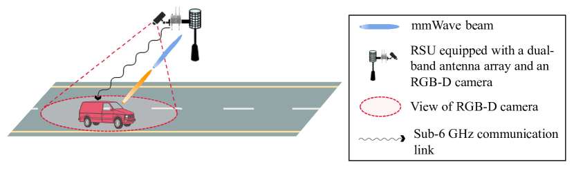
Figure 1: An illustration of the considered V2I scenario model.

II-B Problem Description

To avoid large signaling overhead and latency caused by beam training or tracking methods, RSUs can proactively predict the beamforming angle in the next time slot to formulate a narrow transmit beam that accurately points to the vehicle.

We propose to utilize multi-modal sensory data and wireless channel data to assist the RSU in achieving the above goal. Specifically, RSU senses the traffic environment at a fixed frequency and communicates with the passing vehicle constantly. At the $(n-1)$-th time slot, RSU predicted the relative angle $\hat{\theta}_{n}$ at the passing vehicle using the sequences of RGB images, depth maps, and CSI of sub-6 GHz channel, while the actual angle is denoted by $\theta_{n}$. To achieve this, dedicated pre-processing methods for multi-modal data and feature fusion methods based on DL model need to be developed. Note that the vehicle also needs to formulate the narrow beam that points to RSU based on the angle of the RSU relative to itself when it adopts a MIMO ULA, which is denoted by $\phi_{n}$. For simplicity but without loss of generality, we assume the vehicle drives parallel to the RSU’s antenna array. Then, it follows $\theta_{n}=\phi_{n},{\forall}n$. Therefore, we omit $\phi_{n}$ in this paper and assume that RSU conducts the angle prediction and sends the result to the vehicle instantly within the current downlink transmission block to ensure the link establishment at the next time instance. With the angle prediction result $\hat{\theta}_{n}$, both the RSU and vehicle accordingly formulate the narrow beams using the transmit beamforming matrix $\mathbf{f}_{n}=\mathbf{a}(\hat{\theta}_{n})$ and receive beamforming matrix $\mathbf{w}_{n}=\mathbf{b}(\hat{\theta}_{n})$, respectively. $\mathbf{a}(\theta)$ and $\mathbf{b}(\theta)$ are the transmit steering vector of the RSU’s antenna array and receive steering vector of the vehicle’s antenna array, respectively. The goal of a desirable proactive beamforming scheme is to predict the future relative angle as accurately as possible and maintain stable results when facing realistic random behavior, thus maximizing the achievable rate and reducing the outage probability of the communication system. This could be mathematically expressed as

$$\mathop{\max}\limits_{\mathbf{\Theta}}\ R_{n}(\mathbf{\Theta})=\log_{2}(1+{\rm SNR}_{n}(\hat{\theta}_{n}))$$ (1)

$$s.t.\quad\hat{\theta}_{n}=f_{\mathbf{\Theta}}(\mathbf{h}_{n-2}^{\rm{P}^{\prime}},\mathbf{h}_{n-1}^{\rm{P}^{\prime}},\hat{\mathbf{X}}^{\rm{P}}_{n-2},\hat{\mathbf{X}}^{\rm{P}}_{n-1},\hat{\mathbf{Y}}^{\rm{P}}_{n-2},\hat{\mathbf{Y}}^{\rm{P}}_{n-1})$$

where $f_{\mathbf{\Theta}}(\cdot)$ is the proposed MMFF-Net model; $\mathbf{\Theta}$ is the set of model parameters; $\mathbf{h}_{n-1}^{{\rm{P}}^{\prime}}$, $\hat{\mathbf{X}}^{\rm{P}}_{n-1}$, and $\hat{\mathbf{Y}}^{\rm{P}}_{n-1}$ are the ultimate pre-processed CSI matrix, RGB image, and depth map at the $(n-1)$-th time instance, respectively.

III Multi-Modal Feature Extraction

While serving the passing vehicle, RSU continuously senses the traffic environment. At each slot, it proactively predicts the future position of the vehicle and optimizes beamforming using multi-modal sensory data and wireless channel data. However, multi-modal data has distinct semantic information and data formats, which calls for dedicated data pre-processing and feature extraction that relate to vehicle motion parameters. To address this, we design a novel MMFF-Net consisting of three distinct feature extraction modules, each utilizing different data pre-processing methods and containing NNs with distinct architectures and functions. For simplicity, in the following content, all subscripts $n$ refer to certain data at the $n$-th time instance and will not be reiterated.

III-A Angular Feature Extraction Module

CSI can be regarded as the compressed electromagnetic environment characterization, which is roughly characterized by the relative angle at the passing vehicle. Therefore, we define the angular feature related to the line-of-sight (LoS) channel’s azimuth. Benefiting from the angular feature, the NN can learn the vehicle’s motion state evolution characteristics more efficiently and predict the future position more accurately.

However, obtaining the angular feature faces challenges. First, the MIMO and OFDM techniques jointly lead to a large CSI matrix which causes the high processing load of NN and long training time. Second, the acquisition of CSI in mmWave bands requires excessive signaling overhead and time to transmit sufficient training symbols due to the limited radio frequency (RF) chains in the commonly adopted hybrid structure. Third, raw CSI does not explicitly reflect the angular information of the signal transmission paths though it is a joint result of them. In response to these challenges, we design an angular feature extraction (AFE) module to pre-process the raw CSI into a low-dimensional one and extract the implied angular feature. To avoid the excessive signaling overhead and latency, we assume that RSU obtains the CSI through necessary control signaling (such as synchronous signal) transmitted at sub-6 GHz bands. Though MIMO beamforming is conducted at mmWave bands, CSI at lower frequencies still reflects extremely similar signal propagation process with that of mmWave bands, especially the LoS component [35, 36]. Existing studies [38, 39, 37] also prove such a correlation by predicting the optimal mmWave downlink beam directly from sub-6 GHz channels. Moreover, the co-existing sub-6 GHz and mmWave antenna structure has also appeared in academia and industry [40]. Considering these facts, we propose to use CSI of sub-6 GHz bands to provide rough angular information of vehicle in the electromagnetic domain. In what follows, we will introduce the pre-processing methods of raw CSI and the extraction of the angular feature.

III-A1 Pre-Processing of Raw CSI

The proposed CSI pre-processing method in the AFE module is dedicated to transforming the primitive CSI matrix into a representation with explicit angular features, which is composed of three steps.

Step 1: Beam energy calculation and dimensionality reduction. The size of sub-6 GHz antenna arrays is typically small. In this case, using a conventional discrete Fourier transform (DFT) codebook to calculate the energy of CSI at different beam angles can only provide extremely rough directional information due to the limited number of steering vectors therein. Therefore, we adopt a super-resolution DFT codebook $\mathbf{D}=\left\{\mathbf{d}_{1},\mathbf{d}_{2},...,\mathbf{d}_{\rm{B}}\right\}$ to calculate the total energy of all subcarriers at each beam angle, where $\mathbf{d}_{\rm{b}}\in\mathbb{C}^{N^{\rm{LF}}_{\rm{t}}\times 1}$ and $B$ denote the $b$-th steering vector and angle resolution, respectively. Let $\mathbf{H}_{n}[k]\in\mathbb{C}^{N^{\rm{LF}}_{\rm{t}}\times 1}$ be the sub-6 GHz channel at the $k$-th subcarrier, and $\mathbf{h}_{n}^{\rm{P}}\in\mathbb{R}^{B\times 1}$ be the processed CSI matrix after energy calculation and dimensionality reduction. Then, $\mathbf{h}_{n}^{\rm{P}}[i]$ is represented as:

$$\mathbf{h}_{n}^{\rm{P}}[i]=\frac{1}{K_{\rm{LF}}}\sum_{k=1}^{K_{\rm{LF}}}\log_{2}{(1+\rho\lvert\mathbf{d}_{i}^{\rm{T}}\mathbf{H}_{n}[k]\rvert^{2})}$$ (2)

where $\rho$ denotes the SNR. As the steering angle gets closer to the relative angle between the RSU and the vehicle, the achievable rate increases. Since all subcarriers share the same beam eigenvectors [41], averaging achievable rates across all subcarriers as in (2) will help increase the reliability in identifying the effective beams from $\mathbf{h}_{n}^{\rm{P}}$.

Step 2: Major beam detection by orthogonal matching pursuit (OMP). The use of super-resolution DFT codebook can significantly improve the accuracy of the potential azimuth information of the main signal propagation paths. However, such information cannot be directly obtained by identifying the beam indices with top-$k$ highest energy from $\mathbf{h}_{n}^{\rm{P}}$. This is because of the beam energy dispersion jointly caused by the large number of beam energy generated by the super-resolution DFT codebook and the limited number of actual beams generated by the sub-6 GHz antenna array. To address this issue, we propose to apply the OMP over the $\mathbf{h}_{n}^{\rm{P}}$ to coarsely identify the major beams. The pseudo-code of this method is presented in Algorithm 1.

Algorithm 1 Major Beam Detection by OMP

0:  Processed CSI matrix $\mathbf{h}_{n}^{\rm{P}}$, Original CSI matrix $\mathbf{H}_{n}$, Number of major beams to be detected $G$.

0:  Major beam index set $\mathcal{I}$

1:  Initialization: The residual $\mathbf{R}_{n}=\mathbf{H}_{n}$, beam energy vector $\hat{\mathbf{h}}_{n}^{\rm{P}}=\mathbf{h}_{n}^{\rm{P}}$, and $\mathcal{I}=\emptyset$.

2:  for $j=1:G$ do

3:     $m_{j}=\mathop{\arg\max}\limits_{i}\hat{\mathbf{h}}_{n}^{\rm{P}}[i],i\in[1,B]$

4:     $\mathcal{I}=\{\mathcal{I},m_{j}\}$

5:     $\hat{\mathbf{D}}=\mathbf{D}[:,{\mathcal{I}}]$, $\hat{\mathbf{H}}_{n}^{\rm{a}}=\mathbf{H}_{n}^{\rm{a}}[\mathcal{I},:]$

6:     $\mathbf{R}_{n}=\mathbf{R}_{n}-(\hat{\mathbf{D}}^{\rm{T}})^{\dagger}\hat{\mathbf{H}}_{n}^{\rm{a}}$

7:     for $q=1:B$ do

8:        $\hat{\mathbf{h}}_{n}^{\rm{P}}[q]=\frac{1}{K_{\rm{LF}}}\sum_{k=1}^{K_{\rm{LF}}}\log_{2}{(1+\rho\lvert\mathbf{d}_{q}^{\rm{T}}\mathbf{R}_{n}[k]\rvert^{2})}$

9:     end for

10:  end for

11:  Return the detected major beam index set $\mathcal{I}$.

Step 3: Exclusion of negligible beams. Note that only $k$ major beams are detected in Step 2. To highlight the angular feature and boost the NN’s learning capability, the corresponding elements in $\mathbf{h}_{n}^{\rm{P}}$ are retained and the other elements are set to $0$. We refer to this operation as exclusion of negligible beams. The rationality of this operation will be demonstrated in the next subsection. The ultimate pre-processed CSI matrix $\mathbf{h}_{n}^{{\rm{P}}^{\prime}}\in\mathbb{R}^{B\times 1}$ is expressed as

$$\mathbf{h}_{n}^{{\rm{P}}^{\prime}}[i]=\left\{\begin{array}[]{cl}\mathbf{h}_{n}^{\rm{P}}[i]&,~{}i\in\mathcal{I}\\ 0&,~{}otherwise\end{array}\right.$$ (3)

III-A2 Angular Feature Extraction

Following the above pre-processing, $\mathbf{h}_{n}^{{\rm{P}}^{\prime}}$ is regarded as the wireless part of the multi-modal input data. To extract the angular feature from $\mathbf{h}_{n}^{{\rm{P}}^{\prime}}$, the AFE module adopts the multilayer perceptron (MLP) architecture which contains $L_{\rm{A}}$ layers. Let $\bm{\nu}_{n}$ be the angular feature. $\bm{\nu}_{n}$ is obtained by

$$\bm{\nu}_{n}=\text{MLP}_{\rm A}(\mathbf{h}_{n}^{{\rm{P}}^{\prime}},\mathbf{\Theta}_{\rm A})=\varphi_{\rm A}^{L_{\rm A}}(\varphi_{\rm A}^{L_{\rm A}-1}(...\varphi_{\rm A}^{1}(\mathbf{h}_{n}^{{\rm{P}}^{\prime}})...))$$ (4)

where $MLP_{\rm{A}}$ represents the MLP network, $\mathbf{\Theta}_{\rm{A}}=\left\{\mathbf{W}_{\rm{A}},\mathbf{b}_{\rm{A}}\right\}$ represents its weights and bias, and $\varphi_{\rm{A}}^{l}(\cdot)$ represents the non-linear function of the $l$-th layer. $\varphi_{\rm{A}}^{1}$ can be expressed as

$$\varphi_{\rm A}^{1}(\mathbf{h}_{n}^{{\rm{P}}^{\prime}})=f_{\text{ReLU}}(\mathbf{W}_{\rm{A}}^{1}\mathbf{h}_{n}^{{\rm{P}}^{\prime}}+\mathbf{b}_{\rm{A}}^{1})$$ (5)

where $\mathbf{W}_{\rm{A}}^{1}$ and $\mathbf{b}_{\rm{A}}^{1}$ represent the weight and bias of the first layer. $f_{\rm{ReLU}}(\cdot)$ represents the ReLU function and can be expressed as $f_{\rm{ReLU}}(x)=\max(0,x)$.

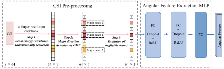
Figure 2: Processing flow for the AFE module.

For clarity, Fig. 2 shows the processing flow of the AFE module, where the CSI is first pre-processed and the angular feature is then extracted. As shown in Fig. 2, the proposed AFE MLP consists of three hidden layers and one output layer. Let $L_{\rm{A}}$ be the number of neurons in the output layer which is also the size of the angular feature and can be adaptively adjusted.

III-A3 Top-K Versus All

The validity of prior CSI pre-processing is demonstrated via “Top-K Versus All” criterion. Specifically, the energy of the $i$-th beam (corresponding to the $i$-th steering vector) is given by $e_{i}={\|(\mathbf{d}_{i}^{\rm{T}})^{\dagger}(\mathbf{D}^{\rm{T}}\mathbf{R}_{n})[i]\|_{\rm{F}}^{2}}$. Then, the proportion of the sum of the top-$k$ major beam energy to the total energy is computed. As shown in Fig. 3, the proportion dramatically increases as the number of selected major beams $k$ increases from $0$ to $2$. This can be attributed to the presence of a few main propagation paths between the RSU and the vehicle, with the total energy of the major beams whose directions are close to these paths accounting for the majority of the total energy. When $k$ becomes larger than $2$, the curve soon saturates, implying the power contributed by the remaining beams becomes negligible. As can be seen in Fig. 3, the top-$2$ beams account for $97.9\%$ of the total energy. Thus, they can be extracted as the latent features to streamline the processing with minimal performance loss.

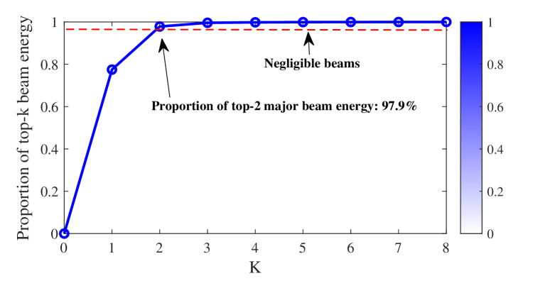
Figure 3: Proportion of the top-$k$ major beam energy to the total energy.

III-B 2D-Visual Feature Extraction Module

As mentioned in Section III-A, CSI provides compressed electromagnetic environment information, and the angular feature potentially indicates the relative angle of the passing vehicle through LoS channel’s azimuth. However, the location information of the vehicle provided by angular feature is relatively rough, calling for a more explicit and adequate environmental awareness as a complement. Images can visually show the location and surrounding environment of the vehicle. The global visual features of the 2D environment provided by images can benefit the localization of the vehicle and the prediction of the future position. The 2D-visual features can supplement relevant information in a non-RF format, such as the locations of scatterers. To efficiently extract the 2D-visual feature, a 2D-visual feature extraction (VFE) module is incorporated into the MMFF-Net.

III-B1 RGB Image Pre-processing

Let $\mathbf{X}_{n}\in\mathbb{R}^{H\times W\times C}$ be the input image of the NN, where $H$, $W$ and $C$ represent the height, width and the number of color channels of the image, respectively. To adjust the values of the features in the RGB image to a similar range, the Z-score normalization is adopted to normalize the three channels of the input RGB images as

$$\hat{\mathbf{X}}_{n}^{(j)}=\frac{\mathbf{X}_{n}^{(j)}-\mu_{n}^{(j)}}{\sigma_{n}^{(j)}},j=1,2,3$$ (6)

where $\hat{\mathbf{X}}_{n}^{(j)}$ is the $j$-th normalized channel, $\mu_{n}^{(j)}$ and $\sigma_{n}^{(j)}$ are the mean value and the standard deviation of the pixel value in the $j$-th channel, respectively. Then, the normalized RGB images are resized to $224\times 224$ to reduce unnecessary computation for NN since there is plenty of redundant information in the original images.

III-B2 2D-Visual Feature Extraction

After the Z-score normalization and resizing operations, $\hat{\mathbf{X}}_{n}^{\rm{P}}$ is regarded as the visual part of the multi-modal input data. In the computer vision field, many powerful NNs have been designed for image feature extraction and analysis [42], serving tasks like target detection and tracking (e.g., Res-Net [43] and AlexNet [44]). To efficiently extract the deep feature of RGB images, the ResNet-18 [43] is adopted in VFE module for its capability of extracting more abundant features while simplifying the learning difficulty and preventing the vanishing gradient issue. Note that the adopted ResNet-18 is customized to adaptively adjust the size of the extracted 2D-visual feature in the MMFF-Net. Specifically, its output fully connected (FC) layer is replaced by one with customized length $L_{\rm{V}}$ which also represents the length of the 2D-visual feature. For clarity, the processing flow for VFE module is shown in Fig. 4.

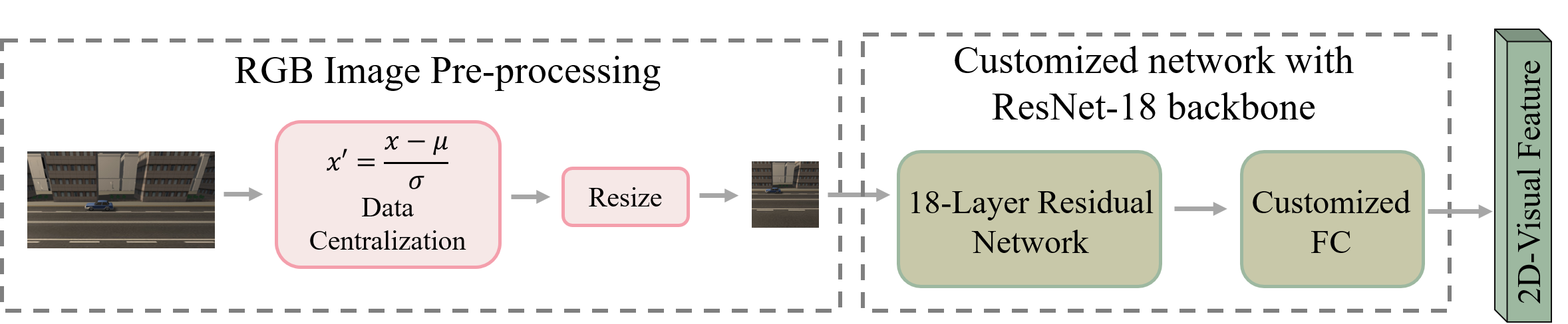
Figure 4: Processing flow for the VFE module.

III-C Distance Feature Extraction Module

Distance information is critical for accurate position prediction, but the AFE and VFE modules do not provide precise distance information. This lack of information limits the ability to reconstruct the 3D environment and predict the vehicle’s exact position. To address this issue, we propose incorporating radar ranging results as an essential sensing modality that naturally complements the semantic information of RGB images by providing 3D geometric shapes for 2D-visual information. To address the lack of radar data in the ViWi dataset, we simulate radar sensing by adding Gaussian noise to depth maps. While the amount of distance data in simulation exceeds that of actual radar ranging, our goal is to showcase the benefits of incorporating distance information in position prediction. We will describe the pre-processing of depth maps and the extraction of distance features in the distance feature extraction (DFE) module.

III-C1 Depth Map Pre-processing

At present, the processing methods of depth map is generally regarding it as an additional channel of the RGB image. This pre-processing approach is not adopted in DFE module. The reasons are as follows. First, the commonly adopted approach assumes that the distance data is accurate and perfectly aligned with RGB image pixels, which is difficult to achieve by practical radar sensing. Second, distance data in depth maps are used to mimic frequent radar ranging results in this scheme. The multi-modal feature extraction and fusion method needs to be universal to radars of various operating frequencies in practical applications. To this end, the depth map is treated as an independent data source.

To boost the learning performance of the MMFF-Net, the order of magnitude of input multi-modal data needs to be approximately the same. Also, the values of features within the depth map need to be aligned comparably. To this end, the min-max normalization is adopted to normalize the input depth map. Let $\mathbf{Y}_{n}$, $\hat{\mathbf{Y}}^{\rm{P}}_{n}$, and $\mathbf{Z}$ be the raw, the pre-processed depth map, and Gaussian noise with zero mean and variance $N_{0}$, respectively. $N_{0}$ is set as $0.1$ in this paper. Then, the $\hat{\mathbf{Y}}^{\rm{P}}_{n}$ is obtained as

$$\hat{\mathbf{Y}}^{\rm{P}}_{n}=\frac{(\mathbf{Y}_{n}+\mathbf{Z})-\min(\mathbf{Y}_{n}+\mathbf{Z})}{\max(\mathbf{Y}_{n}+\mathbf{Z})-\min(\mathbf{Y}_{n}+\mathbf{Z})}$$ (7)

III-C2 Distance Feature Extraction

The radar ranging results are spatially-independent discrete values. In order to make the frequent radar ranging results reflect the overall spatial structure of the environment, the radar ranging results are arranged in the form of images according to the ranging direction. In this scheme, the depth map is equivalent to the radar ranging results with spatial correlation.

Similar to the VFE module, the ResNet-18 is adopted and customized in DFE module to adaptively adjust the size of the extracted distance feature. The output FC layer of ResNet-18 is replaced by one with length $L_{\rm{D}}$ which also represents the length of distance feature. For clarity, the processing flow for DFE module is shown in Fig. 5.

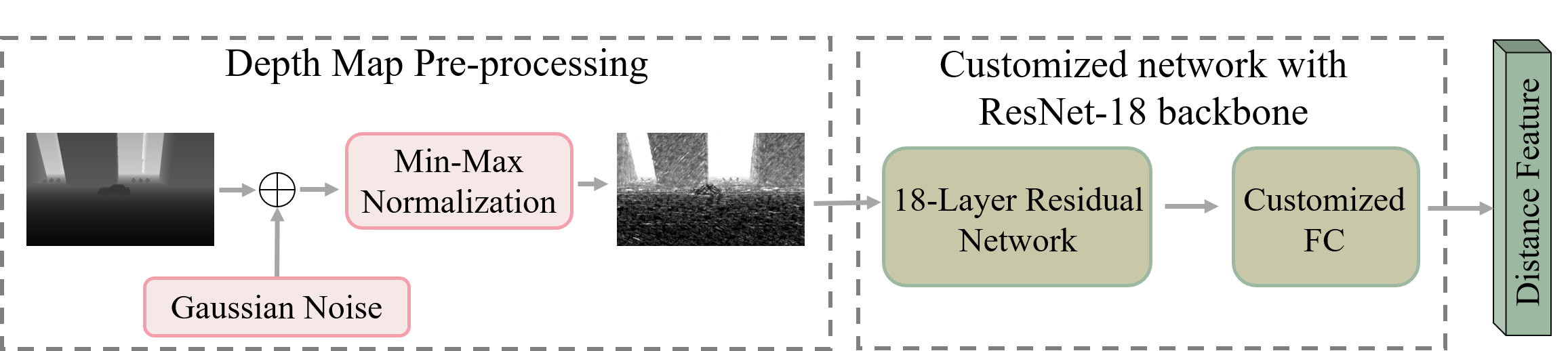
Figure 5: Processing flow for the DFE module.

IV Multi-Modal Feature Fusion and Beamforming Angle Prediction

In this section, we will introduce the adaptive weighted fusion method for combining the angular feature, 2D-visual feature, and distance feature. Following that, we will elaborate on how to proactively predict the beamforming angle based on the two regression models in the MMFF-Net.

IV-A Adaptive Weighted Fusion of Multi-Modal Feature

The multi-modal data used in this scheme contains completely different semantic information. The 2D-visual feature, distance feature, and angular feature need to be preserved entirely to prevent the mixing of different features. Therefore, a tensor concatenation operation is first applied to combine the three features and create an informative representation of the multi-modal feature.

Let ${\rm{AFE}}$, ${\rm{VFE}}$, and ${\rm{DFE}}$ represent the feature extraction processing of the proposed AFE module, VFE module, and DFE module, respectively. Let $\bm{\nu}_{n}$, $\mathbf{\chi}_{n}$, $\bm{\tau}_{n}$, and $\mathbf{f}_{n}$ represent the angular feature, 2D-visual feature, distance feature, and multi-modal feature, respectively. Then, the multi-modal feature $\mathbf{f}_{n}$ can be obtained through (8a) - (8d)

$$\bm{\nu}_{n}={\rm{AFE}}(\mathbf{h}_{n}^{\rm{P}^{\prime}})$$ (8a)

$$\bm{\chi}_{n}={\rm{VFE}}(\hat{\mathbf{X}}^{\rm{P}}_{n})$$ (8b)

$$\bm{\tau}_{n}={\rm{DFE}}(\hat{\mathbf{Y}}^{\rm{P}}_{n})$$ (8c)

$$\mathbf{f}_{n}=\bm{\nu}_{n}\oplus\bm{\chi}_{n}\oplus\bm{\tau}_{n}$$ (8d)

However, treating different features as equally important may potentially lead to performance loss. Therefore, we introduce an adaptive weight learning network (AWLN) module in the MMFF-Net to learn and assign appropriate weights to the multi-modal features. Let $\varphi_{\rm{w}}^{l}(\cdot)$ be the non-linear function of the $l$-th layer in AWLN module with ReLU serving as the activation function. $\varphi_{\rm{w}}^{l}(\cdot)$ is similarly defined as in (5). Then the weight vector $\mathbf{w}_{n}$ output by AWLN can be expressed as

$$\mathbf{w}_{n}=f_{\rm{Sig}}(\mathbf{W}_{\rm{L}}(\varphi_{\rm{w}}^{2}(\varphi_{\rm{w}}^{1}(\mathbf{f}_{n})))+\mathbf{b}_{\rm{L}})$$ (9)

where $\mathbf{W}_{\rm{L}}$ and $\mathbf{b}_{\rm{L}}$ are the weight and bias of the last FC layer in the AWLN module; $f_{\rm{Sig}}(\cdot)$ is the Sigmoid function and can be expressed as $f_{\rm{Sig}}(x)=\frac{1}{1+e^{-x}}$. $f_{\rm{Sig}}(\cdot)$ is served as the activation function of the last FC layer to ensure that the values in the weight vector are between $0$ and $1$.

In fact, the intra-modality weight difference can be omitted and we only need to focus on the inter-modality weight difference. Therefore, we calculate the mean values of the angular feature weight, 2D-visual feature weight, and distance feature weight from the weight vector $\mathbf{w}_{n}$, denoted by $w_{\rm{A}}$, $w_{\rm{V}}$, and $w_{\rm{D}}$, respectively. They are calculated by $w_{\rm{A}}=\frac{1}{L_{\rm{A}}}\sum_{i=1}^{L_{\rm{A}}}\mathbf{w}_{n}(i)$, $w_{\rm{V}}=\frac{1}{L_{\rm{V}}}\sum_{i=1+L_{\rm{A}}}^{L_{\rm{A}}+L_{\rm{V}}}\mathbf{w}_{n}(i)$, and $w_{\rm{D}}=\frac{1}{L_{\rm{D}}}\sum_{i=1+L_{\rm{A}}+L_{\rm{V}}}^{L_{\rm{A}}+L_{\rm{V}}+L_{\rm{D}}}\mathbf{w}_{n}(i)$. Then, we adopt a modality-wise product to obtain the weighted multi-modal feature $\mathbf{f}_{n}^{\rm{w}}$:

$$\mathbf{f}_{n}^{\rm{w}}=w_{\rm{A}}\bm{\nu}_{n}\oplus w_{\rm{V}}\bm{\chi}_{n}\oplus w_{\rm{D}}\bm{\tau}_{n}$$ (10)

For clarity, the processing flow for AWLN module is depicted in Fig. 6. The weighted multi-modal features $\mathbf{f}_{n}^{\rm{w}}$ and $\mathbf{f}_{n-1}^{\rm{w}}$ are then input into the X-axis prediction MLP and Y-axis recurrent prediction module to predict the beamforming angle, as elaborated in the next subsection.

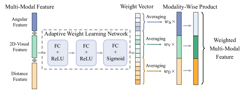
Figure 6: Processing flow for the multi-modal feature fusion module.

IV-B Beamforming Angle Prediction

In the studied scenario, the vehicle is allowed to drift laterally rather than moving in an ideal straight lane. The vehicle’s position tracking is equivalent to the 2D coordinate $(\hat{x}_{{n}+1},\hat{y}_{{n}+1})$ prediction of the vehicle. Assume that the vehicle keeps moving in a straight lane on the $x$-axis, and drifts laterally with a certain probability on the $y$-axis.

IV-B1 Temporal Feature Extraction and Recurrent Prediction for Y-Coordinates Prediction

When the KF-based and the EKF-based state tracking schemes are applied to irregular motion scenarios, the tracking results when the motion state changes have large errors. The motion parameters of vehicles naturally exhibit correlation at adjacent time slots and the correlation tends to decrease with the increase of time interval. Consequently, we propose to extract the temporal feature of the vehicle’s movement and conduct recurrent prediction of the vehicle’s $y$-coordinates. By learning the short-term features of the vehicle’s movement from the historical multi-modal data, there will be no large error in the coordinate prediction results when the vehicle drifts laterally.

Long short-term memory and gated recurrent unit (GRU) networks were designed to solve the problem of vanishing gradient in recurrent neural networks for time series prediction [45]. In the MMFF-Net, GRU is adopted to extract the temporal feature of the vehicle’s movement and conduct the recurrent prediction. Assume that each GRU layer contains $T_{\rm{u}}$ GRU units. The input to the GRU layers in the MMFF-Net consists of sequences of weighted multi-modal features, denoted as $\mathbf{f}^{\rm{w}}_{1,2,\cdots,T_{\rm{u}}}$. Then, the output of the GRU layers can be expressed as

$$\bm{O}_{(T_{\rm{u}})}=F_{\rm{GRU}}(\mathbf{f}_{\rm{1}}^{\rm{w}},\mathbf{f}_{\rm{2}}^{\rm{w}},\cdots,\mathbf{f}_{(T_{\rm{u}})}^{\rm{w}})$$ (11)

GRU utilizes the update gate and reset gate to control the flow of information and determines the update of the hidden state. Given the page limit, the relationships between the input sequences $\mathbf{f}_{1,2,\cdots,T_{\rm{u}}}^{\rm{w}}$ and output $\bm{O}_{(T_{\rm{u}})}$ are not detailed in this paper. We only give the relationship between $\bm{O}_{(T_{\rm{u}})}$, which is also the output of the last unit, and other information as follows

$$\bm{O}_{(T_{\rm{u}})}=(1-\bm{z}_{(T_{\rm{u}})})\otimes\bm{O}_{(T_{\rm{u}}-1)}+\bm{z}_{(T_{\rm{u}})}\otimes\widetilde{\bm{O}}_{(T_{\rm{u}})}$$ (12)

where $\bm{z}_{(T_{\rm{u}})}$ is the value of the $T_{\rm{u}}$-th update gate in GRU and $\widetilde{\bm{O}}_{(T_{\rm{u}})}$ is the information retained by the $T_{\rm{u}}$-th unit.

IV-B2 MLP Prediction for X-Coordinates Prediction

The prediction of the vehicle’s $x$-coordinates is carried out by a four-layer MLP rather than a recurrent NN, since the feature of the vehicle’s movement on the $x$-axis is easily learned by NN. This design ensures prediction accuracy while reducing the computational load and accelerating the convergence of NN.

With the predicted vehicle’s 2D coordinate, the beamforming angle in the next time instance $\hat{\theta}_{n+1}$ can be determined by $\hat{\theta}_{n+1}=\arctan(\frac{\hat{x}_{{n}+1}-x_{RSU}}{\hat{y}_{{n}+1}})$ with $x_{RSU}$ being the x-coordinate of the RSU. For clarity, Fig. 7 shows the overall block diagram of the MMFF-Net.

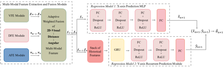
Figure 7: The proposed MMFF-Net is composed of three main modules: (i) multi-modal feature extraction and fusion module; (ii) Y-axis recurrent prediction module; and (iii) X-axis prediction MLP.

Remark 1: The proposed MMFF-Net can be extended to multi-user scenarios. By allocating orthogonal subcarriers to different vehicles, the system can differentiate between them and effective angular features can be extracted from CSI matrices corresponding to different subcarriers. In the VFE module, multi-object detection and tracking algorithms can distinguish multiple vehicles and the DFE module can obtain their ranging information.

V Experimental Setup

This section introduces the evaluation dataset and metrics, as well as the network architecture and training methodology for MMFF-Net.

V-A Dataset Overview

The dataset used for testing is based on the ViWi data-generation framework [34]. The “dist_cam” scenario acts as the basis, where a single car drives through a city street. The hyper-parameters for channel generation are presented in Table I. We simulate the sub-6 GHz CSI based on the wireless channel parameters provided by ViWi dataset. To emulate the rich multi-path components in sub-6 GHz band, we reset the path gains while keeping the other parameters of paths unchanged such as angle of arrival (AoA) and time of arrival (ToA). The parameters of the LoS component remain unchanged, assuming that there are two paths with a $2-5$ dB random gain reduction compared to the LoS component and three paths with a $5-10$ dB random gain reduction. The rationality of this methodology is supported by a comprehensive channel measurement campaign conducted in diverse scenarios [36], which indicated that the geometries of main propagation paths of two frequency bands are almost similar. Furthermore, to make the dataset more realistic, the vehicle is assumed to randomly move to adjacent lanes during its movement. The complete trajectory remains continuous except for some time instances of lane changing. This randomness can also be regarded as the vehicle’s drifting. Fig. 8 displays an example of the vehicle’s trajectory where it randomly drifts. For the construction of training and testing datasets, we randomly generate two entirely different trajectories, where the vehicle’s drifting behaviors occur randomly and differently.

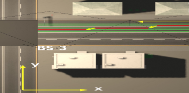
Figure 8: An example of the vehicle’s trajectory where the vehicle randomly drifts. This example is constructed based on the “dist_cam” scenario.

TABLE I: Hyper-parameters for channel generation

Parameter	mmWave Band	Sub-6 GHz Band
Scenario name	dist_cam
Active BSs	1
Codebook size $B$	64
Transmit antennas (x, y, z)	(8/16/32,1,1)	(8,1,1)
Receive antennas (x, y, z)	(8/16/32,1,1)	(1,1,1)
Bandwidth (GHz)	–	0.08
Antenna spacing	0.5
OFDM sub-carriers	–	64
OFDM limit	–	32
Paths	–	15

V-B Signal Model

At the $n$-th epoch, RSU sends a downlink directional data stream $s_{n}(t)$ to the vehicle using beamforming matrix $\mathbf{f}_{n}\in\mathbb{C}^{N^{\rm{HF}}_{\rm{t}}\times 1}$ (equivalent to the transmit beamformer for the single vehicle). The beamforming matrix $\mathbf{f}_{n}$ is designed based on the intended direction. Assume that the beamforming direction $\hat{\theta}_{n}$ is already obtained by the proposed scheme, the beamforming matrix is given by $\textbf{f}_{n}=\mathbf{a}(\hat{\theta}_{n})$, with $\mathbf{a}(\theta)=\frac{1}{\sqrt{N^{\rm{HF}}_{\rm{t}}}}[1,e^{-{\rm{j}}\pi\cos\theta},\cdots,e^{-{\rm{j}}\pi(N^{\rm{HF}}_{\rm{t}}-1)\cos\theta}]^{\rm{T}}$ representing the transmit steering vector of RSU’s antenna array, which is assumed to adopt half-wavelength antenna spacing. Likewise, let $\mathbf{b}(\theta)=\frac{1}{\sqrt{M^{\rm{HF}}_{\rm{r}}}}[1,e^{-{\rm{j}}\pi\cos\theta},\cdots,e^{-{\rm{j}}\pi(M^{\rm{HF}}_{\rm{r}}-1)\cos\theta}]^{\rm{T}}$ be the receive steering vector.

At the $n$-th epoch, the vehicle forms a receive beamformer $\mathbf{w}_{n}$ according to the predicted angle to receive the signals transmitted by RSU. The receive signal is expressed as [16]

$$c_{n}(t)=\tilde{\kappa}\sqrt{p_{n}}\alpha_{n}e^{{\rm{j}}2\pi\mu_{n}t}\mathbf{w}_{n}^{\rm{H}}\mathbf{b}(\theta_{n})\mathbf{a}^{\rm{H}}(\theta_{n})\mathbf{f}_{n}s_{n}(t)+z_{\rm{c}}(t)$$ (13)

where $p_{n}$ is the transmit power; $\tilde{\kappa}=\sqrt{N_{\rm{t}}^{\rm{HF}}M_{\rm{r}}^{\rm{HF}}}$ is the antenna array gain; $\alpha_{n}$ is the reflection coefficient, $z_{\rm{c}}(t)$ is the Gaussian noise term which has zero mean and variance $\sigma_{\rm{c}}^{2}$. $\textbf{w}_{n}=\mathbf{b}(\hat{\theta}_{n})$ is the receive beamformer that the vehicle prepares according to the predicted relative angle between the vehicle and RSU at the $n$-th epoch. $\mu_{n}$ denotes the Doppler frequency and is affected by the vehicle’s velocity $v_{n}$, relative angle with RSU $\theta_{n}$, and carrier frequency $f_{\rm{c}}$, i.e., $\mu_{n}=\frac{v_{n}\cos\theta_{n}f_{\rm{c}}}{c}$. $\alpha_{n}=\tilde{\alpha}d_{n}^{-1}e^{{\rm{j}}\frac{2\pi f_{\rm{c}}}{c}d_{n}}$ denotes the LoS channel coefficient. $\tilde{\alpha}$ representing the reference power gain factor which is assumed to be known to RSU by calculating the channel power gain at the reference distance and $\frac{2\pi f_{\rm{c}}}{c}d_{n}$ represents the phase of the LoS channel.

Suppose that the transmit signal has a unit power, then the SNR of the signal received by the vehicle is given by ${\rm SNR}_{n}=\frac{p_{n}{\lvert\tilde{\kappa}\alpha_{n}\mathbf{b}(\hat{\theta}_{n})^{\rm{H}}\mathbf{b}(\theta_{n})\mathbf{a}^{\rm{H}}(\theta_{n})\mathbf{a}(\hat{\theta}_{n})\rvert}^{2}}{\sigma^{2}_{\rm{c}}}$. The achievable rate of the established link is given by $R_{n}=\log_{2}(1+{\rm SNR}_{n})$. As discussed above, the achievable rate depends on the transmit and receive beamformers, which are designed based on the predicted relative angle between the vehicle and RSU. The achievable rate is maximized if the predicted beamforming angle is perfectly consistent with the actual angle, i.e., $\theta_{n}=\hat{\theta}_{n}$, yielding a SNR upper bound as ${\rm SNR}_{\rm{max}}=\frac{p_{n}{\lvert\tilde{\kappa}\alpha_{n}\rvert}^{2}}{\sigma^{2}_{\rm{c}}}$.

V-C Network Configuration

Table II shows the hyper-parameters used for designing the network, including the sizes of multi-modal features and the architecture details of multiple NN modules in the MMFF-Net. The size of angular feature is set smaller than the others since the vehicle’s position information it contains may not be as intuitive and reliable as that present in visual and distance features, especially in complex environments. In terms of NN architectures, we evaluated NNs with various depths and widths, and then determined the architecture used in this paper based on their performance and computational complexity. The AFE MLP has two hidden layers and one output layer, with all dropout layers having a deactivation rate of $0$. The X-axis prediction MLP has three hidden layers and one output layer, with all dropout layers having a deactivation rate of $p=0$. The Y-axis recurrent prediction module has two layers of GRUs, each with $r$ GRU units. The MLP connected to the second GRU layer has two hidden layers and one output layer, with two dropout layers having a deactivation rate of $p=0.1$. Table III lists the hyper-parameters used for fine-tuning the model. The training of MMFF-Net is performed by PyTorch, using the adaptive moment estimation (ADAM) optimizer [46].

TABLE II: Hyper-parameters for network design

Parameter	Value
The size of multi-modal features@[$L_{\rm{A}}$, $L_{\rm{V}}$, $L_{\rm{D}}$]	[16, 256, 256]
GRU units per layer $r$	16
Neurons in hidden layers of AFE MLP@[layer1, layer2, layer3]	[64, 32, 16]
Neurons in hidden layers of X-axis prediction MLP@[layer1, layer2, layer3, layer4]	[528, 256, 128, 64]
Neurons in hidden layers of Y-axis recurrent prediction module@[layer1, layer2, layer3]	[16, 32, 16]
Neurons in hidden layers of AWLN module@[layer1, layer2, layer3]	[528, 264, 528]

TABLE III: Hyper-parameters for network fine-tuning

Parameter	Value
Batch size	[1, 5, 10]
Learning rate	$3\times 10^{-4}$
Learning rate scheduler	Epochs 15 and 30
Learning-rate decaying factor	0.3
Epochs	50
Optimizer	ADAM
Loss funtion	SmoothL1Loss

V-D Benchmarks

In this paper, extensive simulation results are provided and comprehensive comparisons between the proposed scheme with several existing benchmarks are conducted. In order to highlight the superiority and importance of multimodality fusion, three uni-modal data based schemes are designed and fine-tuned to perform the same proactive beamforming task.

• KF-based tracking (KF-T): A typical KF is adopted to track the vehicle’s motion parameters, where ground truth values added with noises serve as the observation values.

• EKF-based tracking (EKF-T) [18]: In [18], an EKF-based method is proposed where the observation values are the transmit signal echoes. The state variables are the vehicle’s position and velocity, as well as the channel coefficient. The vehicle is assumed to move in an ideal straight line in the considered scenario.

• Dual-functional radar-communication (DFRC) aided tracking (DFRC-T) [19]: In [19], an EKF-based method is proposed where the DFRC signals are used for probing the target to avoid dedicated pilots. The state variables used are different from those in EKF-T. The vehicle is also assumed to move in an ideal straight lane.

• DL-based predictive beamforming (DL-PB) [22]: In [22], an FC network is designed to estimate the current angular parameter and calculate the beamforming angle at the next time slot based on the state evolution model established on the ideal straight lane. The echoes of DFRC signals are used as network input.

• Vision-aided mmWave beam prediction (V-A-BP) [25]: In [25], the proactive beamforming task is degenerated to an image classification one and RGB images are utilized to predict the optimal beam from a pre-defined codebook. The images where the vehicle is at similar positions are classified into one category. Consequently, RSU uses the same beam to communicate with the vehicle at similar positions, which inevitably leads to the deviation of beam alignment.

• Image-aided predictive beamforming (I-PB): A uni-modal data based scheme that utilizes images to predict the vehicle position is designed. The I-PB scheme is designed to explore the role and effect of the 2D-visual feature for vehicle position prediction. Therefore, apart from the absence of data from the other two modalities and their respective NN modules, the image parameters, data processing methods, and network architecture of I-PB are identical to those of MMFF-Net.

• Depth map-aided predictive beamforming (D-PB): A uni-modal data based scheme that utilizes depth maps to predict the vehicle position is designed. The D-PB scheme is designed to explore the role and effect of the distance feature for vehicle position prediction. Similar with I-PB, the only difference between D-PB and MMFF-Net is the absence of CSI and images.

• CSI-aided predictive beamforming (C-PB): A uni-modal data based scheme that utilizes CSI to predict the vehicle position is designed. Note that the mapping between CSI and the vehicle’s absolute coordinates is difficult to fit through NN since CSI represents the compressed electromagnetic environment feature and the vehicle’s position is just one of the contributing factors. Therefore, a temporal-difference prediction scheme is designed. That is, the NN predicts the displacement of vehicles at adjacent time slots through the potential angle variation feature in CSI sequences. The CSI data and its processing methods have not been changed.

VI Performance Evaluation

In this section, extensive simulation results are presented to verify the effectiveness and superiority of the proposed scheme over the benchmarks. All the simulation results presented are on the average of $300$ independent realizations.

VI-A Angle Prediction

First, the angle prediction performances of the proposed MMFF-Net and benchmarks are given in Fig. 9. To present the results more clearly, the relative errors are presented instead of the absolute prediction results. The EKF-T and DFRC-T periodically utilize the received radar echoes at BS as the measurement signal vector, which causes excessive signaling overhead. However, the MMFF-Net does not consume extra communication overhead to detect vehicle’s motion status periodically, thereby saving extensive spectrum resources. The angle tracking error of the KF-T is large due to its inapplicability in the non-linear motion model. The performance of DFRC-T is slightly better than that of EKF-T. The minimum angle prediction error of DFRC-T is $3.75\times 10^{-2}$ when $N_{\rm{t}}^{\rm{HF}}=M_{\rm{r}}^{\rm{HF}}=8$ but it is still $74.41\%$ higher than that of MMFF-Net. While the EKF-T and DFRC-T methods can initially achieve relatively accurate prediction results during the early stages of the tracking process, their errors gradually accumulate over time, causing the predicted angles to deviate from the actual angle, as depicted in Fig. 9. This deviation ultimately leads to the failure of beam tracking, which will be discussed in the next subsection. By contrast, the MMFF-Net consistently maintains stable and accurate prediction performance throughout the tracking process.

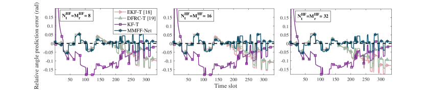
Figure 9: Angle prediction performance comparisons among MMFF-Net, KF-T, EKF-T [18], and DFRC-T [19] schemes.

Fig. 10 shows the angle tracking performances of MMFF-Net, DL-PB [22], and V-A-BP schemes [25]. The hyper-parameters for the network design and fine-tuning given in [22, 25] are adopted in our simulations. The equivalent angle prediction values corresponding to the beam prediction results of V-A-BP are obtained, which are finite discrete values due to the codebook with finite angular resolution. As can be seen in Fig. 10, the V-A-BP can only complete rough angle tracking with relatively large errors, especially when the vehicle approaches the RSU. The DL-PB can hardly realize effective tracking of the vehicle since it merely relies on limited received signals and simple NN architecture.

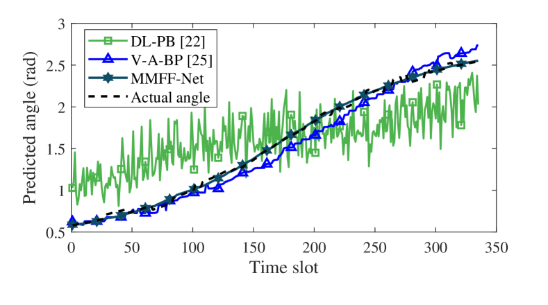
Figure 10: Angle prediction performance comparisons among MMFF-Net, DL-PB [22], and V-A-BP [25] schemes.

To further illustrate the necessity and superiority of multimodality fusion, the angle prediction performance of MMFF-Net and uni-modal schemes is presented in Table IV. The angle prediction errors of C-PB and D-PB is larger than EKF-T, which indicates that merely relying on the angular feature and distance feature is not sufficient for accurate vehicle tracking. Among the uni-modal schemes, the I-PB scheme performs the closest to the MMFF-Net but its average prediction error is still $9.77\%$ higher and the standard deviation of error is $21.20\%$ higher. Furthermore, when the vehicle approaches RSU, the angle prediction error of I-PB is $1.99\times 10^{-2}$ and $32.67\%$ higher than that of MMFF-Net, demonstrating its weaker tracking ability for fast-varying angles. The performance gain brought by the proposed AWLN module can be reflected through the reduction in mean and standard deviation of angle prediction error, highlighting the significance of weight allocation among distinct multi-modal features.

From the discussions above, it can be concluded that the superior performance of MMFF-Net is attributed to the efficient extraction of diverse behavioral features from multi-modal data that complement each other and reflect the vehicle’s motion parameters more comprehensively and the thoughtful design of feature extraction and fusion mechanisms. Despite the increased complexity, MMFF-Net is first trained offline and then deployed on high-performance RSU for online operation. Therefore, the increased complexity does not pose significant difficulties in MMFF-Net’s practical application.

TABLE IV: Angle prediction performances of MMFF-Net, MMFF-Net w/o AWLN module, and other uni-modal schemes.

Schemes	Mean of angle prediction error (rad)	Standard deviation of angle prediction error (rad)
I-PB	$2.36\times 10^{-2}$	$2.23\times 10^{-2}$
D-PB	$3.30\times 10^{-2}$	$2.71\times 10^{-2}$
C-PB	$7.15\times 10^{-2}$	$5.70\times 10^{-2}$
MMFF-Net w/o AWLN	$2.18\times 10^{-2}$	$1.85\times 10^{-2}$
MMFF-Net	$2.15\times 10^{-2}$	$1.84\times 10^{-2}$

VI-B Achievable Rate

In Fig. 11, the achievable rate comparisons between MMFF-Net and several benchmark schemes are shown. The transmit power $p_{n}$ is set to $15$dB. In the simulation scenario, the vehicle travels from one side of the RSU to the other, and the distance between them decreases first and then increases. Consequently, most of the achievable rates increase first, reach the maxima when the vehicle passes RSU, and then decrease, as can be observed in Fig. 11. Furthermore, the average achievable rates increase as $N_{\rm{t}}^{\rm{HF}}$ and $M_{\rm{r}}^{\rm{HF}}$ increase thanks to the corresponding increased array gain. As shown in Fig. 11, the MMFF-Net and DFRC-T schemes achieve similar performances in 8-antenna array case, both outperforming the I-PB. In 16-antenna and 32-antenna array cases, the advantage of MMFF-Net over I-PB and EKF-T becomes notable especially in the latter half of the tracking process. The average achievable rates of MMFF-Net, I-PB, and DFRC-T are $8.05$bps/Hz, $7.77$bps/Hz, and $7.48$bps/Hz in 16-antenna array case, and $8.56$bps/Hz, $7.86$bps/Hz, and $6.30$bps/Hz in 32-antenna array case, respectively. It is worth noting that the V2I link that DFRC-T establishes is extremely unstable in the latter half of the tracking process since the linearization assumption and the approximation of the model in EKF algorithm causes error accumulation issue when dealing with highly nonlinear models, which severely limits its practical application effectiveness. However, MMFF-Net can effectively avoid this issue thanks to its powerful capability in handling nonlinear relationships and its characteristic of not requiring an explicit prior model. In the latter half of the tracking process, the average achievable rates of DFRC-T are $6.80$bps/Hz and $3.52$bps/Hz in 16 and 32-antenna array cases, while those of MMFF-Net are $8.12$bps/Hz and $8.77$bps/Hz.

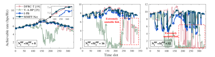
Figure 11: Achievable rate performance comparisons among MMFF-Net, DFRC-T [19], V-A-BP [25], and I-PB schemes.

Fig. 11 also presents the effect of vehicle drifting on achievable rate performance. The drifting behavior is realized by randomly generating a trajectory from discrete points on five parallel lanes, which is an abrupt event without any sign. Therefore, neither the uni-modal schemes nor the proposed scheme can predict such an event. All schemes experience a notable rate decrease due to misalignment in drifting, as observed in Fig. 11.

It is noteworthy that adding antennas does not necessarily ensure an increasing achievable rate. Despite the high array gain, a larger array generates a narrower beam, which is likely to miss the target vehicle and thus leads to a larger beam misalignment probability. As shown in Fig. 11, the achievable rates of the DFRC-T, I-PB, and MMFF-Net for the 16-antenna array case are higher than those of 8-antenna array case since their angle prediction accuracy can meet the alignment accuracy demand of 16-antenna array case. However, the angle prediction results of all schemes are not accurate enough to align the narrow beam generated by the 32-antenna array when the vehicle drifts, thereby causing the 32-antenna array case to perform worse than the 16-antenna array case in terms of achievable rates when the vehicle drifts.

VI-C Outage Probability

To evaluate the improvement of the proposed proactive beamforming scheme on the system’s outage capacity, we analyze the outage probability for different proactive beamforming approaches. Let $P(R_{\rm{T}})$ be the outage probability when $R_{\rm{T}}$ is the minimum required achievable rate, $R_{n}$ be the achievable rate at the $n$-th time slot, $N(R_{\rm{T}})$ be the total number of time slots that meet the minimum achievable rate demand, and $N$ be the total number of time slots, then

$$P(R_{\rm{T}})=1-\frac{N(R_{\rm{T}})}{N}$$ (14a)

$$N(R_{\rm{T}})=\sum_{n=0}^{N}{\chi(R_{n},R_{\rm{T}})}$$ (14b)

$$\chi(R_{n},R_{\rm{T}})=\left\{\begin{array}[]{cl}1&,~{}R_{n}\geq R_{\rm{T}}\\ 0&,~{}\mathrm{otherwise}\end{array}\right.\par$$ (14e)

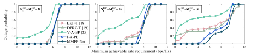
Figure 12: Comparisons of outage probability performance among MMFF-Net, EKF-T [18], DFRC-T [19], V-A-BP [25], and I-PB schemes.

Fig. 12 demonstrates the proposed scheme has a lower outage probability than other schemes, with the superiority becoming evident as $N_{\rm{t}}^{\rm{HF}}$ and $M_{\rm{r}}^{\rm{HF}}$ increase. As discussed in Section VI-B, a larger antenna does not necessarily lead to an increasing achievable rate since the narrower beam is more likely to miss the target vehicle. This conclusion can also be confirmed by the outage probability of the communication system. As shown in Fig. 12, the outage probability of the 32-antenna array case is larger than that of 16-antenna array case when using the MMFF-Net, under a minimum achievable rate requirement of $4.80$-$7.60$bps/Hz. DFRC-T achieves slightly higher achievable rates when the vehicle is very close to the RSU thanks to the abundant measurements with large-size antennas. This leads to a lower outage probability when the required minimum rate is higher than $8.00$bps/Hz and $9.90$bps/Hz in 16 and 32-antenna array cases. However, for the overall tracking process, the outage probability is minimized when adopting MMFF-Net. MMFF-Net achieves a reduction of $1.36\%$, $5.90\%$, and $19.43\%$ in the outage probability compared to DFRC-T in 8, 16, 32-antenna array cases, and $1.12\%$, $2.88\%$, and $5.97\%$ compared to I-PB.

VI-D Robustness Testing Against Adverse Environmental Conditions

TABLE V: Achievable rate performance of MMFF-Net confronted with adverse environmental conditions.

Schemes $(N_{\rm{t}}^{\rm{HF}},M_{\rm{r}}^{\rm{HF}})=(8,16,32)$	Mean of achievable rates	Maximum of achievable rates	Minimum of achievable rates
MMFF-Net	(6.41, 8.05, 8.56)	(7.43, 9.24, 10.49)	(5.48, 6.95, 4.86)
MMFF-Net confronted with adverse environment conditions	(6.31, 7.72, 7.88)	(7.26, 8.65, 9.76)	(5.44, 5.20, 1.86)

The MMFF-Net system may encounter scenarios with varying degrees of errors in multi-modal data due to adverse environmental conditions. To assess the model’s performance and robustness in such real-world scenarios, we manually introduce noise to the testing set simulating sensing device errors caused by environmental interference. Firstly, we reduce the RGB image brightness to simulate poor lighting conditions. Secondly, we introduce channel estimation errors to the CSI to simulate a non-ideal communication environment. The errors are measured using average normalized mean squared error (NMSE) and are set to $-15$dB. The NMSE is defined by ${\rm NMSE}=\frac{\|\hat{\mathbf{H}}_{n}-\mathbf{H}_{n}\|_{\rm{F}}^{2}}{\|\mathbf{H}_{n}\|_{\rm{F}}^{2}}$, with $\hat{\mathbf{H}}_{n}$ representing the CSI with errors. Thirdly, we increase the variance of the Gaussian noise added to the depth map to $1$ to simulate distance measurement errors due to weather factors. Then, the testing dataset is used to test the robustness of the MMFF-Net model pre-trained with the normal training set and the results are shown in Table V. The MMFF-Net inevitably experiences performance degradation and its average achievable rates are lower than those of I-PB and MMFF-Net in normal environment condition but are $3.21\%$ and $25.08\%$ higher than those of DFRC-T in 16 and 32-antenna array cases. Therefore, the pre-trained MMFF-Net model exhibits robustness in maintaining a reliable V2I communication link even in the presence of environmental interference, demonstrating its reliable network architecture as well as strong feature extraction and fusion capabilities.

VII Conclusions

In this paper, we presented a novel proactive beamforming scheme for V2I links that leverages multi-modal sensing and communication integration. Our proposed scheme takes advantage of the complementary nature of multi-modal environment information and captures distinct features of the surrounding environment. To effectively extract and fuse the multi-modal features implied by the multi-modal data, we designed a novel MMFF-Net capable of pre-processing the multi-modal data with distinct data structures in the form of time series. To demonstrate the applicability of the proposed scheme to complex and dynamic scenarios, we constructed a dataset using the ViWi data-generation framework and enriched it by considering the vehicle’s drifting behavior. We compared our proposed scheme with eight representative methods and revealed it can outperform all in terms of angle prediction accuracy, achievable rate, and outage performance. Moreover, our proposed scheme possesses the strongest robustness against vehicle drifting and environmental interference, demonstrating its practicality and effectiveness in complex dynamic scenarios. For future work, we aim to refine the CSI pre-processing at lower frequencies and extend the MMFF-Net to multi-vehicle scenarios.

References

- [1] W. Xu et al., “Internet of Vehicles in big data era,” IEEE/CAA J. Automat. Sinica, vol. 5, no. 1, pp. 19–35, Jan. 2018.
- [2] N. Lu, N. Cheng, N. Zhang, X. Shen, and J. W. Mark, “Connected Vehicles: Solutions and Challenges,” IEEE Internet Things J., vol. 1, no. 4, pp. 289–299, Aug. 2014.
- [3] X. Cheng, D. Duan, S. Gao, and L. Yang, “Integrated Sensing and Communications (ISAC) for Vehicular Communication Networks (VCN),” IEEE Internet Things J., vol. 9, no. 23, pp. 23441–23451, Dec. 2022.
- [4] S. Chen et al., “Vehicle-to-Everything (v2x) Services Supported by LTE-Based Systems and 5G,” IEEE Commun. Stand. Mag., vol. 1, no. 2, pp. 70–76, 2017.
- [5] X. Cheng, S. Gao, and L. Yang, mmWave Massive MIMO Vehicular Communications. Springer, Nature, Switzerland, 2022.
- [6] F. Boccardi, R. W. Heath, A. Lozano, T. L. Marzetta, and P. Popovski, “Five disruptive technology directions for 5G,” IEEE Commun. Mag., vol. 52, no. 2, pp. 74–80, Feb. 2014.
- [7] F. Rusek, D. Persson, B. K. Lau, E. G. Larsson, T. L. Marzetta, O. Edfors, and F. Tufvesson, “Scaling Up MIMO: Opportunities and Challenges with Very Large Arrays,” IEEE Signal Process. Mag., vol. 30, no. 1, pp. 40–60, Jan. 2013.
- [8] K. V. Mishra, M. R. B. Shankar, V. Koivunen, B. Ottersten, and S. A. Vorobyov, “Toward millimeter wave joint radar-communications: A signal processing perspective,” IEEE Signal Process. Mag., vol. 36, no. 5, pp. 100–114, Sep. 2019.
- [9] O. El Ayach, S. Rajagopal, S. Abu-Surra, Z. Pi, and R. W. Heath, “Spatially Sparse Precoding in Millimeter Wave MIMO Systems,” IEEE Trans. Wireless Commun., vol. 13, no. 3, pp. 1499–1513, Mar. 2014.
- [10] S. Gao, X. Cheng, and L. Yang, “Mutual Information Maximizing Wideband Multi-User (wMU) mmWave Massive MIMO,” IEEE Trans. Commun., vol. 69, no. 5, pp. 3067–3078, May. 2021.
- [11] T. Van Luong, N. Shlezinger, C. Xu, T. M. Hoang, Y. C. Eldar, and L. Hanzo, “Deep Learning Based Successive Interference Cancellation for the Non-Orthogonal Downlink,” IEEE Trans. Veh. Technol., vol. 71, no. 11, pp. 11876–11888, Nov. 2022.
- [12] J. Wang et al., “Beam codebook based beamforming protocol for multi-Gbps millimeter-wave WPAN systems,” IEEE J. Sel. Areas Commun., vol. 27, no. 8, pp. 1390–1399, Oct. 2009.
- [13] Z. Xiao, T. He, P. Xia, and X.-G. Xia, “Hierarchical Codebook Design for Beamforming Training in Millimeter-Wave Communication,” IEEE Trans. Wireless Commun., vol. 15, no. 5, pp. 3380–3392, May. 2016.
- [14] V. Va, H. Vikalo, and R. W. Heath, “Beam tracking for mobile millimeter wave communication systems,” in 2016 IEEE Global Conference on Signal and Information Processing (GlobalSIP), Washington, DC, USA, Dec. 2016, pp. 743–747.
- [15] A. Alkhateeb, O. El Ayach, G. Leus, and R. W. Heath, “Channel Estimation and Hybrid Precoding for Millimeter Wave Cellular Systems,” IEEE J. Sel. Top. Sign. Proces., vol. 8, no. 5, pp. 831–846, Oct. 2014.
- [16] S. Gao, X. Cheng, and L. Yang, “Estimating Doubly-Selective Channels for Hybrid mmWave Massive MIMO Systems: A Doubly-Sparse Approach,” IEEE Trans. Wireless Commun., vol. 19, no. 9, pp. 5703–5715, Sep. 2020.
- [17] X. Cheng, Z. Huang, and L. Bai, “Channel Nonstationarity and Consistency for Beyond 5G and 6G: A Survey,” IEEE Commun. Surveys Tutor., vol. 24, no. 3, pp. 1634–1669, 3rd Quart., 2022.
- [18] S. Shaham, M. Ding, M. Kokshoorn, Z. Lin, S. Dang, and R. Abbas, “Fast Channel Estimation and Beam Tracking for Millimeter Wave Vehicular Communications,” IEEE Access, vol. 7, pp. 141104–141118, 2019.
- [19] F. Liu, W. Yuan, C. Masouros, and J. Yuan, “Radar-Assisted Predictive Beamforming for Vehicular Links: Communication Served by Sensing,” IEEE Trans. Wireless Commun., vol. 19, no. 11, pp. 7704–7719, Nov. 2020.
- [20] W. Yuan, F. Liu, C. Masouros, J. Yuan, D. W. K. Ng, and N. González-Prelcic, “Bayesian Predictive Beamforming for Vehicular Networks: A Low-Overhead Joint Radar-Communication Approach,” IEEE Trans. Wireless Commun., vol. 20, no. 3, pp. 1442–1456, Mar. 2021.
- [21] W. Yuan, Z. Wei, S. Li, J. Yuan, and D. W. K. Ng, “ Integrated Sensing and Communication-Assisted Orthogonal Time Frequency Space Transmission for Vehicular Networks,” IEEE J. Sel. Top. Sign. Proces., vol. 15, no. 6, pp. 1515–1528, Nov. 2021.
- [22] J. Mu, Y. Gong, F. Zhang, Y. Cui, F. Zheng, and X. Jing, “Integrated Sensing and Communication-Enabled Predictive Beamforming With Deep Learning in Vehicular Networks,” IEEE Commun. Lett., vol. 25, no. 10, pp. 3301–3304, Oct. 2021.
- [23] C. Liu, W. Yuan, S. Li, X. Liu, H. Li, D. K. Ng, and Y. Li, “Learning-Based Predictive Beamforming for Integrated Sensing and Communication in Vehicular Networks,” IEEE J. Sel. Areas Commun., vol. 40, no. 80, pp. 2317–2334, Aug. 2022.
- [24] F. Liu and C. Masouros, “A Tutorial on Joint Radar and Communication Transmission for Vehicular Networks—Part III: Predictive Beamforming Without State Models,” IEEE Commun. Lett., vol. 25, no. 2, pp. 332–336, Feb. 2021.
- [25] M. Alrabeiah, A. Hredzak, and A. Alkhateeb, “Millimeter Wave Base Stations with Cameras: Vision-Aided Beam and Blockage Prediction,” in Proc. VTC-Spring, Antwerp, Belgium, May. 2020, pp. 1–5.
- [26] U. Demirhan and A. Alkhateeb, “Radar Aided 6G Beam Prediction: Deep Learning Algorithms and Real-World Demonstration,” in Proc. WCNC, Austin, TX, USA, Apr. 2022, pp. 2655–2660.
- [27] A. Klautau, N. González-Prelcic, and R. W. Heath, “LIDAR Data for Deep Learning-Based mmWave Beam-Selection,” IEEE Wireless Commun. Lett., vol. 8, no. 3, pp. 909–912, Jun. 2019.
- [28] S. Wu, C. Chakrabarti, and A. Alkhateeb, “LiDAR-Aided Mobile Blockage Prediction in Real-World Millimeter Wave Systems,” in Proc. WCNC, Austin, TX, USA, Apr. 2022, pp. 2631–2636.
- [29] G. Charan, M. Alrabeiah, and A. Alkhateeb, “Vision-Aided 6G Wireless Communications: Blockage Prediction and Proactive Handoff,” IEEE Trans. Veh. Technol., vol. 70, no. 10, pp. 10193–10208, Oct. 2021.
- [30] Y. Fan, S. Gao, D. Duan, X. Cheng, and L. Yang, “Radar Integrated MIMO Communications for Multi-Hop V2V Networking,” IEEE Wireless Commun. Lett., vol. 12, no. 2, pp. 307–311, Feb. 2023.
- [31] W. Xu, F. Gao, X. Tao, J. Zhang, and A. Alkhateeb, “Computer Vision Aided mmWave Beam Alignment in V2X Communications,” IEEE Trans. Wireless Commun., vol. 22, no. 4, pp. 2699-2714, Apr. 2023.
- [32] F. Liu et al., “Integrated Sensing and Communications: Towards Dual-Functional Wireless Networks for 6G and Beyond,” IEEE J. Sel. Areas Commun., vol. 40, no. 6, pp. 1728–1767, Jun. 2022.
- [33] X. Cheng et al., “Intelligent Multi-Modal Sensing-Communication Integration: Synesthesia of Machines,” IEEE Commun. Surveys Tuts., early access, doi: 10.1109/COMST.2023.3336917.
- [34] M. Alrabeiah, A. Hredzak, Z. Liu, and A. Alkhateeb, “ViWi: A Deep Learning Dataset Framework for Vision-Aided Wireless Communications,” in Proc. IEEE 91st Vehicular Technol. Conf. (VTC2020-Spring), Antwerp, Belgium, May. 2020, pp. 1–5.
- [35] A. Ali, N. González-Prelcic, and R. W. Heath, “Estimating millimeter wave channels using out-of-band measurements,” in Proc. Inf. Theory Appl. Workshop (ITA), La Jolla, California, USA, 2016, pp. 1–6.
- [36] M. Peter et al., “Measurement campaigns and initial channel models for preferred suitable frequency ranges, deliverable D2.1,” mmMAGIC Project, Tech. Rep., 2016. [Online]. Available: https://bscw.5g-mmmagic.eu/pub/bscw.cgi/d94832/mmMAGIC_D2-1.pdf
- [37] F. Gao, B. Lin, C. Bian, T. Zhou, J. Qian, and H. Wang, “FusionNet: Enhanced Beam Prediction for mmWave Communications Using Sub-6 GHz Channel and a Few Pilots,” IEEE Trans. Commun., vol. 69, no. 12, pp. 8488–8500, Dec. 2021.
- [38] M. S. Sim, Y.-G. Lim, S. H. Park, L. Dai, and C.-B. Chae, “Deep Learning-Based mmWave Beam Selection for 5G NR/6G With Sub-6 GHz Channel Information: Algorithms and Prototype Validation,” IEEE Access, vol. 8, pp. 51634–51646, 2020.
- [39] M. Alrabeiah and A. Alkhateeb, “Deep Learning for mmWave Beam and Blockage Prediction Using Sub-6 GHz Channels,” IEEE Trans. Commun., vol. 68, no. 9, pp. 5504–5518, Sep. 2020.
- [40] Qualcomm Announces Successful Data Calls Using 5G mmWave and Sub-6 GHz Aggregation. Accessed: Apr. 13, 2021. [Online]. Available: https://www.qualcomm.com/news/releases/2021/04/13/qualcommannounces-successful-data-calls-using-5g-mmwave-and-sub-6-ghz.
- [41] A. Alkhateeb and R. W. Heath, “Frequency Selective Hybrid Precoding for Limited Feedback Millimeter Wave Systems,” IEEE Trans. Commun., vol. 64, no. 5, pp. 1801–1818, May. 2016.
- [42] J. Ngiam, A. Khosla, M. Kim, J. Nam, H. Lee, and A. Ng, “Multimodal deep learning,” in Proc. 28th Int. Conf. Mach. Learn. (ICML), Jan. 2011, pp. 689–696.
- [43] K. He, X. Zhang, S. Ren, and J. Sun, “Deep Residual Learning for Image Recognition,” in Proc. IEEE Conf. Comput. Vis. Pattern Recognit. (CVPR), Jun. 2016, pp. 770–778.
- [44] A. Krizhevsky, I. Sutskever, and G. E. Hinton, “ImageNet Classification with Deep Convolutional Neural Networks,” in Proc. Int. Conf. Neural Inf. Process. Syst. (NIPS), Dec. 2012, pp. 1097–1105.
- [45] I. Goodfellow, Y. Bengio, and A. Courville, Deep Learning. Cambridge, MA, USA: MIT Press, 2016.
- [46] D. P. Kingma and J. Ba, “Adam: A method for stochastic optimization,” in Proc. Int. Conf. Learn. Representations, 2015.