ISAC Signal Processing Over Unlicensed
Spectrum Bands

Abstract

As a promising key technology of 6th-Generation (6G) mobile communication systems, integrated sensing and communication (ISAC) technology aims to make full use of spectrum resources to enable the functional integration of communication and sensing. The ISAC-enabled mobile communication systems regularly operate in non-continuous spectrum bands due to crowded licensed frequency bands. However, the conventional sensing algorithms over non-continuous spectrum bands have disadvantages such as reduced peak-to-sidelobe ratio (PSR) and degraded anti-noise performance. Facing this challenge, we propose a high-precision ISAC signal processing algorithm based on compressed sensing (CS) in this paper. By integrating the resource block group (RBG) configuration information in 5th-Generation new radio (5G NR) and channel information matrices, we can dynamically and accurately obtain power estimation spectra. Moreover, we employ the fast iterative shrinkage-thresholding algorithm (FISTA) to address the reconstruction problem and utilize K-fold cross validation (KCV) to obtain optimal parameters. Simulation results show that the proposed algorithm has lower sidelobes or even zero sidelobes and high anti-noise performance compared with conventional sensing algorithms.

I Introduction

TABLE I: Abbreviations and Notations

Abbreviation	Description	Abbreviation	Description
5G-A	5th-Generation-Advanced	6G	6th-Generation
5G NR	5th-Generation New Radio	5G NR-U	5th-Generation New Radio-Unlicensed
2D	Two-Dimensional	AWGN	Additive White Gaussian Noise
ADC	Analog-to-digital Converter	CS	Compressed Sensing
CP	Cyclic Prefix	CR	Cognitive Radio
DFT	Discrete Fourier Transform	DAC	Digital-to-Analog Converter
FFT	Fast Fourier Transform	FISTA	Fast Iterative Shrinkage-Thresholding Algorithm
JCMSA	Joint CS and Machine Learning ISAC Signal Processing Algorithm	IDFT	Inverse Discrete Fourier Transform
IFFT	Inverse Fast Fourier Transform	ISAC	Integrated Sensing and Communication
KCV	K-fold Cross Validation	LTE-U	Long Term Evolution-Unlicensed
MM	Majorization-Minimization	MU-MIMO	Multi-User Multi-Input Multi-Output
NC-OFDM	Non-Continuous OFDM	NP	Non-deterministic Polynomial-time
P/S	Parallel-to-Serial Converter	PSR	Peak-to-Sidelobe Ratio
RBG	Resource Block Group	RX	Receiver
RIP	Restricted Isometry Property	RMSE	Root Mean Square Error
S/P	Serial-to-Parallel Converter	SNR	Signal-to-Noise Ratio
SI	Subcarrier Interleaving	TX	Transmitter
Notation	Description	Notation	Description
${N_{\text{c}}}$	Total number of subcarriers	$\Omega$	Available subcarriers set
$n\in\Omega$	Sequence number of an available subcarrier in total $N_{\text{c}}$	$n^{\prime}$	The $n^{\prime}$-th subcarrier, $n^{\prime}\in\left\{1,2,\cdots,N_{\text{c}}\right\}$
${M_{\text{sym}}}$	Total number of OFDM symbols	$T_{\text{sym}}$	Entire symbol duration
$T_{\text{cp}}$	CP length	$T_{\text{ofdm}}$	Elementary symbol duration
$\Delta f$	Subcarrier spacing	$\circ$	Hadamard product
$N_{\text{op}}$	The number of available subcarriers of $m$-th symbol	$\mathbf{A}_{m}$	The spectrum occupancy sequence of $m$-th symbol
$\mathbf{D}_{\text{R}1}$	The channel information matrix without noise in scenario 1	$\mathbf{D}_{\text{V2}}$	The channel information matrix without noise in scenario 2
$\otimes$	Kronecker product	$\mathbf{\Psi},\mathbf{\Upsilon}$	IDFT matrix, DFT matrix
$\mathbf{y}_{m}$	The $m$-th column vector of $\mathbf{D}_{\text{R}1}$	$\mathbf{k}_{n}$	The $n$-th row vector of $\mathbf{D}_{\text{V2}}$
$\mathbf{P}_{m},\mathbf{Q}_{n}$	The power spectra of range and velocity	$\mathbf{J},\mathbf{F}$	The matrix for compressive reconstruction
$\lambda$	The regularization parameter	$\varpi$	The gain produced by FISTA
$(\cdot)^{-1}$	Inverse operation	$(\cdot)^{\text{T}},[\cdot]^{\text{T}}$	Transpose operation
$\|\cdot\|_{0}$	The $\ell_{0}$-norm	$\|\cdot\|_{1}$	The $\ell_{1}$-norm
$\|\cdot\|_{2}$	The $\ell_{2}$-norm	$|\cdot|$	An absolute value

With the emerging typical applications such as smart city and intelligent transportation, the integrated sensing and communication (ISAC) in 5th-Generation-Advanced (5G-A) and 6th-Generation (6G) mobile communication systems aims to integrate sensing services into mobile communication infrastructure. On one hand, compared with separated design of communication and radar sensing, the ISAC system realizes the sharing of hardware and spectrum resources of radar sensing and communication, thus saving spectrum resources and improving hardware efficiency [1, 2]. On the other hand, radar and communication systems have high similarities in hardware architecture, antenna structure, and spectrum band, which provide feasibility for the integrated design of communication and sensing. Therefore, the research on ISAC system has attracted wide attention in academia and industry.

Due to the scarcity of spectrum resources and the requirement to improve the utilization of spectrum bands, cognitive radio (CR) originally proposed by Dr. Joseph Mitola has attracted wide attention [3], where unlicensed spectrum bands are utilized. At present, unlicensed spectrum bands are also used in mobile communication systems, evolving into long term evolution-unlicensed (LTE-U) and 5G new radio-unlicensed (5G NR-U) [4]. Hence, the mobile communication systems enabled by ISAC technology will work in non-continuous spectrum bands. However, the non-continuous of spectrum bands will lead to the degradation of anti-noise performance, resolution, and deterioration of Fourier sidelobes with conventional ISAC signal processing algorithms. Hence, enhancing the sensing capabilities in non-continuous spectrum bands faces significant challenges.

In view of the challenges existing in the ISAC system over non-continuous spectrum bands, it is mainly solved from the aspects of signal design and signal processing, which are summarized as follows.

Signal design: The OFDM pilot signal, being a typical non-continuous signal, has been studied in the perspectives of pilot design and pilot optimization. In terms of pilot design, Chen [5] designed a time-frequency continuous pilot structure with low parameter estimation error and high anti-noise capability. Bao et al. [6] exploited superimposed pilots to realize target sensing with limited energy and high detection probability. In terms of pilot optimization, Liu et al. [7] optimized the pilot structure by minimizing the Cramér-Rao bound in the scenario of single target detection. Tzoreff et al. [8] optimized the pilot matrix by minimizing the maximum eigenvalue of the Cramér-Rao bound. Both of these researches applied the semi-definition relaxation (SDR) to release rank-1 constraint. However, SDR-based optimization algorithm performs poorly on multi-objective detection problems. To address this challenge, Huang et al. [9] replaced the rank-1 constraint with a tight and smooth approximation, and applied the majorization-minimization (MM) method to solve the pilot optimization problem.

Signal processing: Schweizer et al. [10] exploited a stepped OFDM signal for sensing, which is non-continuous in time-frequency domain. Then, the range phase error due to discontinuity is compensated by modifying the standard discrete Fourier transform (DFT). Knill et al. [11] presented frequency-agile sparse OFDM radar and applied a two-dimensional (2D) compressed sensing (CS) method to obtain the complete range-velocity profile. Sturm et al. [12] considered the multi-user multi-input multi-output (MU-MIMO) radar and used equally spaced subcarriers per user to achieve full bandwidth sensing resolution. However, this method has the disadvantage of reduced maximum unambiguous distance. To overcome this disadvantage, Hakobyan et al. [13] used non-equidistant dynamic subcarriers instead of equally spaced subcarriers. Furthermore, an optimized subcarrier interleaving (SI) scheme is proposed to maximize sidelobes reduction while addressing the deteriorating effect of dynamic subcarriers on sidelobes. For the ISAC system working in unlicensed and non-continuous spectrum bands, Wei et al. [14] extracted the configuration information of the resource block group (RBG) in 5G new radio (5G NR) to obtain the spectrum judgment sequence. This sequence is then used to zero the non-data parts of the channel information matrix and perform a 2D fast Fourier transform (2D FFT) to estimate target range and velocity information. Simulation results show that the improved 2D FFT algorithm enhances the anti-noise performance of target estimation in non-continuous spectrum bands. It is obvious that the above studies provide solutions in terms of ISAC signal design and processing under non-continuous spectrum bands. However, the non-continuous spectrum bands cause high Fourier sidelobes and low signal-to-noise ratio (SNR) problems in conventional radar estimation algorithms, and the ISAC signal processing with the capabilities of anti-noise and low sidelobes in dynamic unlicensed spectrum bands is still challenging.

In this paper, we propose a high-precision CS-based ISAC signal processing algorithm combined with machine learning to improve sensing performance. This study focuses on mobile communication systems, adopting OFDM as the ISAC signal, which is the standard signal of mobile communication systems. The OFDM ISAC signals in the non-continuous spectrum bands are collectively referred to as non-continuous OFDM (NC-OFDM) signals. Firstly, we extract the spectrum occupancy sequence from the RBG configuration information in 5G NR and partially zero the channel information matrix according to the processing method in [14]. Then, we apply the proposed CS-based 2D FFT algorithm for parameter estimation on the modified channel information matrix, combine it with machine learning to search for optimal parameters, and ultimately obtain the power spectrum with low sidelobes and high SNR. The main contributions of this paper are summarized as follows.

• CS-based high-precision sensing algorithm: Combining the spectrum occupancy sequence information and CS theory, we transform the target estimation problem into a power spectrum reconstruction problem and use fast iterative shrinkage-thresholding algorithm (FISTA) [15] to solve the optimization problem. Thus, high-precision sensing is achieved under dynamic, stochastic, and non-continuous unlicensed spectrum bands.

• Machine learning-based parameter optimization: The $K$-fold cross validation (KCV) is applied to select the optimal regularization parameter $\lambda$ to realize faster convergence speed and a smaller reconstruction error compared with traditional methods.

• Algorithm superiority: Simulation results show that the proposed CS-based ISAC signal processing algorithm has a higher peak-to-sidelobe ratio (PSR) and better anti-noise performance in non-continuous spectrum bands than the conventional sensing algorithm. We provide the optimal regularization parameter for the SNR between 0 and 10 dB, which results in a power spectrum with zero sidelobes.

The rest of this paper is arranged as follows. Section II introduces the NC-OFDM-based ISAC signal model and CS theory. Section III presents the ISAC signal processing over unlicensed spectrum bands. Section IV reveals the optimal choice of the regular term $\lambda$ and the sensing performance analysis. Section V shows simulation results demonstrating improved anti-noise performance and PSR of target estimation under non-continuous spectrum bands using the proposed algorithm. Finally, this paper is summarized in Section VI. Table I provides a comprehensive list of the abbreviations and notations that are utilized throughout this paper.

II Signal Model and Compressed Sensing

II-A Signal Model

The ISAC signals based on NC-OFDM and continuous OFDM have similar expression form. Assuming that the total number of subcarriers in the NC-OFDM system is $N_{\text{c}}$ and the set of available subcarrier numbers obtained with the assistance of the spectrum sensing module is $\Omega\subseteq\{1,2,\cdots,N_{\text{c}}\}$, the base band transmit signal at the transmitter (TX) is expressed as [16]

$$x\left(t\right)_{\text{\tiny NC-OFDM}}= \sum\limits_{m=1}^{M_{\text{sym}}}\sum\limits_{n=1}^{N_{\text{c}}}d_{m,n}\exp{\left(j2\pi f_{n}t\right)}$$ (1)

$$\times\operatorname{rect}\left(\frac{t-mT_{\text{sym}}}{T_{\text{sym}}}\right),$$

where $m\in\{1,2,\cdots,M_{\text{sym}}\}$ represents the index value of an NC-OFDM symbol in total $M_{\text{sym}}$ NC-OFDM symbols, and $n\in\Omega$ represents the sequence number of an available subcarrier in total $N_{c}$ subcarriers, $T_{\text{sym}}=T_{\text{ofdm}}+T_{\text{cp}}$ is the duration of the entire NC-OFDM symbol, $T_{\text{ofdm}}$ is the elementary NC-OFDM symbol duration, $T_{\text{cp}}$ is the length of cyclic prefix (CP). $d_{m,n}$ is the modulation symbol at the $m$-th NC-OFDM symbol of the $n$-th subcarrier. $f_{n}$ is the frequency of $n$-th subcarrier, which is $n$ times of $\Delta f$ with $\Delta f$ representing the subcarrier spacing [17, 16].

The ISAC signal based on NC-OFDM is reflected on the surface of the target with a range of $R$ and a Doppler frequency shift $f_{\text{D}}=2v_{0}f_{\text{c}}/c$ is generated due to relative motion, where $v_{0}$ represents the relative velocity between the target and TX, $c$ represents the velocity of light, and $f_{\text{c}}$ represents the carrier frequency. Then, the received signal at the receiver (RX) is expressed as [16]

$$y(t)_{\text{\tiny NC-OFDM}}= \sum_{m=1}^{M_{\text{sym}}}\sum_{n=1}^{N_{\text{c}}}\alpha_{m,n}d_{m,n}\exp\left(j2\pi f_{n}(t-\tau)\right)$$ (2)

$$\times\exp\left(j2\pi f_{\text{D}}t\right)\operatorname{rect}\left(\frac{t-mT_{\text{sym}}-\tau}{T_{\text{sym}}}\right),$$

where $\alpha_{m,n}$ represents the channel coefficient at the $m$-th OFDM symbol of the $n$-th subcarrier. $\tau=2R/c$ is the time delay [18]. In [16], the improved signal processing algorithm based on the radar signal processing algorithm in the symbol modulation domain was proposed. In order to highlight the influence of target range and Doppler frequency shift, (2) is rewritten as [16]

$$y(t)_{\text{\tiny NC-OFDM}}= \sum_{m=1}^{M_{\text{sym}}}\exp\left(j2\pi f_{\text{D}}t\right)\sum_{n=1}^{N_{\text{c}}}\alpha_{m,n}$$ (3)

$$\times\left\{d_{m,n}\exp\left(-j2\pi f_{n}\frac{2R}{c}\right)\right\}$$

$$\times\exp\left(j2\pi f_{n}t\right)\operatorname{rect}\left(\frac{t-mT_{\text{sym}}-\frac{2R}{c}}{T_{\text{sym}}}\right).$$

As shown in Fig 1, the spectrum occupancy is dynamically sensed and the available subcarriers are allocated to unlicensed users. At the radar component, the spectrum usage information in the current $N_{\text{c}}$ subcarriers can be obtained through the RBG configuration information module in ISAC system based on NC-OFDM. The output result of spectrum occupancy sequence module can be represented by a spectrum occupancy sequence $\textbf{A}_{m}\in\mathbb{C}^{N_{\text{c}}\times 1}$, where $\textbf{A}_{m}=\left[a_{1,m},a_{2,m},\cdots,a_{N_{\text{c}},m}\right]^{\mathrm{T}}$ and $[\cdot]^{\text{T}}$ represents transpose operation. $a_{i,m}=0$ indicates that the $i$-th subcarrier of the $m$-th symbol is unavailable, and $a_{i,m}=1$ indicates that the $i$-th subcarrier of the $m$-th symbol is available. The number of non-zero elements in $\textbf{A}_{m}$ is $\mathcal{N}_{m}$, and $\mathcal{N}_{m}$ is the number of subcarriers occupied at the $m$-th NC-OFDM symbol. Finally, the radar sensing module integrates information from the element-wise complex division module, the spectrum occupancy sequence module, and the machine learning-based parameter optimization module to estimate the target range and velocity information carried by the reflected signal.

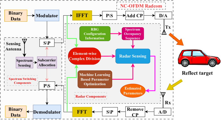
Figure 1: Structure of NC-OFDM ISAC system, with abbreviations CP: cyclic prefix, FFT: fast Fourier transforms, IFFT: inverse fast Fourier transform, ADC: analog-to-digital converter, DAC: digital-to-analog converter, S/P: serial-to-parallel converter, P/S: parallel-to-serial converter.

The spectrum occupancy of NC-OFDM ISAC system is dynamic. Especially, ISAC system works in the unlicensed spectrum bands and the spectrum switching will be performed according to the spectrum switching component. The following research is carried out in two scenarios [19, 20]. It is crucial to note that the band for unlicensed users is called the available band, while the band for licensed users is the unavailable band.

• Scenario 1: The spectrum bands occupied by licensed users and unlicensed users are not switched within the target sensing period.

• Scenario 2: The spectrum bands occupied by licensed users and unlicensed users are switched within the target sensing period.

Given that the study of this paper employs the CS theory, in order to facilitate the understanding of Section III, we briefly introduce the theory of CS in Section II-B.

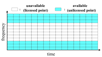
Figure 2: Spectrum occupancy under scenario 1.

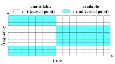
Figure 3: Spectrum occupancy under scenario 2.

II-B Compressed Sensing Theory

CS is a technique for finding sparse solutions to overdetermined linear systems. It allows the recovery of the original signal with high accuracy using a small amount of under-sampled information by solving an optimization problem with a measurement matrix irrelevant to the transformation matrix [21].

Under an orthogonal basis $\psi\in\mathbb{C}^{N\times N}$, the transformation of signal x is $\mathbf{\theta}=(\mathbf{\psi})^{\mathrm{T}}\textbf{x}$, where $(\cdot)^{\text{T}}$ denotes transpose operation. If the number of non-zero elements in the sparse vector $\theta$ is equal to an integer $K$, the sparsity of the signal x is called $K$-sparse. CS is applied to solve the problem of reconstructing the original vector x from the observed vector y, which is given by

$$\textbf{y}=\mathbf{\Phi}\textbf{x}=\textbf{A}\theta,$$ (4)

where $\textbf{y}\in\mathbb{C}^{M\times 1}(M<N)$, $\textbf{x}\in\mathbb{C}^{N\times 1}$, $\mathbf{\Phi}\in\mathbb{C}^{M\times N}$ is a measurement matrix, and $\textbf{A}\in\mathbb{C}^{M\times N}=\mathbf{\Phi}\mathbf{\psi}$ is called sensing matrix. Solving (4) directly is an ill-conditioned problem. If $M\gg K$ and the sensing matrix A satisfies the restricted isometry property (RIP) condition, the problem of (4) can be transformed into the minimum $\ell_{0}$ norm problem, namely

$$\min\limits_{\theta}\|\theta\|_{0}\quad\mathrm{s.t.}\quad\textbf{A}\theta=\textbf{y}.$$ (5)

where $\|\cdot\|_{0}$ represents the $\ell_{0}$-norm.

The above problem is non-deterministic polynomial-time hard (NP-hard) [22]. [23] mentions that the solution of the minimum $\ell_{0}$ norm problem is equivalent to the solution of the minimum $\ell_{1}$ norm problem according to the sparsity of reconstructed signal and the correlation of sensing matrix, namely, the non-convex optimization problem is transformed into a convex optimization problem. Then, (5) is transformed into

$$\min\limits_{\theta}\|\theta\|_{1}\quad\mathrm{s.t.}\quad\textbf{A}\theta=\textbf{y}.$$ (6)

where $\|\cdot\|_{1}$ represents $\ell_{1}$-norm.

In practice, the observed vector y is generally contains noise, so that (4) is transformed into $\textbf{y}=\mathbf{\Phi}\textbf{x}+\varepsilon$, where $\varepsilon$ is additive white Gaussian noise (AWGN). Therefore, (6) is transformed into [24]

$$\min\limits_{\theta}\|\theta\|_{1}\quad\mathrm{s.t.}\quad\|\textbf{A}\theta-\textbf{y}\|_{2}\leqslant\varepsilon.$$ (7)

By solving the above convex optimization problem, we achieve the recovery of the original data from the under-sampled data.

III ISAC Signal Processing over Unlicensed Spectrum Bands

In this section, the ISAC signal processing algorithm over unlicensed spectrum bands is proposed. Specifically, we first describe how to obtain the channel information matrix. Then the estimation algorithms for target’s range and velocity are presented, respectively. We denote this ISAC signal processing method as “Joint CS and Machine Learning ISAC Signal Processing Algorithm”, abbreviated as JCMSA.

In 2011, Sturm et al. [16] proposed the 2D FFT method, which utilizes a 2D Fourier transform to estimate velocity and range of target. Velocity and range estimation can be obtained by the modulation symbols sequence $\mathbf{d}_{\text{TX}}\left(m,n^{\prime}\right)$ and $\mathbf{d}_{\text{RX}}\left(m,n^{\prime}\right)$, where $n^{\prime}\in\left\{1,2,\cdots,N_{\text{c}}\right\}$ represents the $n^{\prime}$-th subcarrier. Upon observing (3), the delay and Doppler frequency shift caused by the target are independent in the modulation symbol. Thus, the modulation symbol on the RX can be expressed as [16]

$$\mathbf{d}_{\text{RX}}\left(mN_{\text{c}},n^{\prime}\right)= \alpha_{m,n^{\prime}}\mathbf{d}_{\text{TX}}\left(mN_{\text{c}},n^{\prime}\right)\exp\left(-j2\pi f_{n}^{\prime}\frac{2R}{c}\right)$$ (8)

$$\times\exp\left(j2\pi mT_{\text{sym}}f_{\text{D}}\right).$$

For a clear representation, the modulation symbols can be converted to the matrix form, where each row represents a subcarrier of the same frequency and each column represents an NC-OFDM symbol. (8) can be expressed as [25]

$$\left(\mathbf{D}_{\text{RX}}\right)_{m,n^{\prime}}=\alpha_{m,n^{\prime}}\left(\mathbf{D}_{\text{TX}}\right)_{m,n^{\prime}}\circ\left(\mathbf{d}_{\text{r}}\otimes\mathbf{d}_{\text{v}}\right)_{m,n^{\prime}},$$ (9)

where $\circ$ denotes Hadamard product, and $\otimes$ denotes Kronecker product. Through an element-wise complex division, the channel information matrix $(\mathbf{D}_{\text{div}})_{m,n^{\prime}}$ is obtained by

$$\left(\mathbf{D}_{\text{div }}\right)_{m,n^{\prime}}=\frac{\left(\mathbf{D}_{\text{Rx}}\right)_{m,n^{\prime}}}{\left(\mathbf{D}_{\text{Tx}}\right)_{m,n^{\prime}}}=\alpha_{m,n^{\prime}}\left(\mathbf{d}_{\text{r}}\otimes\mathbf{d}_{\text{v}}\right)_{m,n^{\prime}},$$ (10)

where the vector $\mathbf{d}_{\text{r}}$ and $\mathbf{d}_{\text{v}}$ can be transformed into

$$\mathbf{d}_{\text{r}}(n^{\prime})=\exp\left(-j2\pi f_{n}^{\prime}\frac{2R}{c}\right),\quad n^{\prime}=1,\ldots,N_{\text{c}}$$ (11)

and

$$\mathbf{d}_{\text{v}}(m)=\exp\left(j2\pi mT_{\text{sym}}\frac{2v_{0}f_{\text{c}}}{c}\right).\quad m=1,\ldots,M_{\text{sym}}$$ (12)

Finally, the target’s range and relative velocity can be obtained by applying (11) and (12) to perform inverse discrete Fourier transform (IDFT) and discrete Fourier transform (DFT) [16].

When the ISAC-based mobile communication systems work on unlicensed spectrum bands with spectrum occupancy as shown in Fig. 2 and Fig. 3, the 2D FFT method shows deterioration in sensing performance. Specifically, the spectrum holes caused by the non-continuous spectrum bands can lead to deterioration of the Fourier sidelobes of the power spectrum and degradation of anti-noise performance [26]. To address the above problem, we proposed a novel algorithm, namely JCMSA, which transforms the power spectrum estimation problem into a compressive reconstruction problem, thereby obtaining lower sidelobes and better anti-noise performance.

III-A Range Estimation Algorithm

First, we use modulation symbol division to obtain the unprocessed channel information matrix. Due to the non-continuous spectrum, the noise power of the unavailable points in the unprocessed channel information matrix is amplified [14]. To reduce the noise, we first extract the RBG configuration information in 5G NR to obtain the spectrum occupancy sequence $\mathbf{A}_{m}$. Then, we combine $\mathbf{A}_{m}$ and the unprocessed channel information matrix to set the unavailable points to zero. The processed channel information matrix $\mathbf{D}_{\text{R1}}$ for scenario 1 is expressed as (23).

In (23),

$$\mathbf{D}_{\text{R1}}=\left[\begin{array}[]{cccc}s_{1,1}+\varepsilon_{1,1}&s_{1,2}+\varepsilon_{1,2}&\cdots&s_{1,M_{\text{sym}}}+\varepsilon_{1,M_{\text{sym}}}\\ s_{2,1}+\varepsilon_{2,1}&s_{2,2}+\varepsilon_{2,2}&\cdots&s_{2,M_{\text{sym}}}+\varepsilon_{2,M_{\text{sym}}}\\ \vdots&\vdots&\ddots&\vdots\\ s_{\frac{\mathcal{N}_{m}}{2},1}+\varepsilon_{\frac{\mathcal{N}_{m}}{2},1}&s_{\frac{\mathcal{N}_{m}}{2},2}+\varepsilon_{\frac{\mathcal{N}_{m}}{2},2}&\cdots&s_{\frac{\mathcal{N}_{m}}{2},M_{\text{sym}}}+\varepsilon_{\frac{\mathcal{N}_{m}}{2},M_{\text{sym}}}\\ 0&0&\cdots&0\\ \vdots&\vdots&\ddots&\vdots\\ 0&0&\cdots&0\\ s_{N_{\text{c}}-\frac{\mathcal{N}_{m}}{2}+1,1}+\varepsilon_{N_{\text{c}}-\frac{\mathcal{N}_{m}}{2}+1,1}&s_{N_{\text{c}}-\frac{\mathcal{N}_{m}}{2}+1,2}+\varepsilon_{N_{\text{c}}-\frac{\mathcal{N}_{m}}{2}+1,2}&\cdots&s_{N_{\text{c}}-\frac{\mathcal{N}_{m}}{2}+1,M_{\text{sym}}}+\varepsilon_{N_{\text{c}}-\frac{\mathcal{N}_{m}}{2}+1,M_{\text{sym}}}\\ \vdots&\vdots&\ddots&\vdots\\ s_{N_{\text{c}},1}+\varepsilon_{N_{\text{c}},1}&s_{N_{\text{c}},2}+\varepsilon_{N_{\text{c}},2}&\cdots&s_{N_{\text{c}},M_{\text{sym}}}+\varepsilon_{N_{\text{c}},M_{\text{sym}}}\end{array}\right],$$ (23)

 

$s_{m,n^{\prime}}$ and $\varepsilon_{m,n^{\prime}}$ denote that the data and noise after the modulation symbols have undergone element-wise complex division. The position of the zero-row vector in $\mathbf{D}_{\text{R1}}$ corresponds to the spectrum occupancy sequence $\textbf{A}_{m}$. From (10), it is obtained that the linear phase shift of range is only along the frequency axis. Therefore, by processing the columns of $\mathbf{D}_{\text{R1}}$, the target’s range information can be obtained.

III-A1 Compressive reconstruction of the power spectrum of range

$\mathbf{D}_{\text{R1}}$ is split into $M_{\text{sym}}$ column vectors, with expressions as follows.

$$\mathbf{D}_{\text{R1}}=\left(\mathbf{y}_{1},\mathbf{y}_{2},\cdots,\mathbf{y}_{m},\cdots,\mathbf{y}_{M_{\text{sym}}}\right),$$ (24)

where $\mathbf{y}_{m}\in\mathbb{C}^{N_{\text{c}}\times 1}$ is the $m$-th column vector of $\mathbf{D}_{\text{R1}}$. According to (23), the position of the zero element in $\mathbf{y}_{m}$ corresponds to the element 0 in $\mathbf{A}_{m}$, which is expressed by

$$\mathbf{y}_{m}=\mathbf{A}_{m}\circ\mathbf{y}_{m(\text{full})},$$ (25)

where $\mathbf{y}_{m(\text{full})}$ represents the $m$-th column vector of the channel information matrix obtained from the OFDM signal that occupies all subcarriers. According to 2D FFT algorithm, the power spectrum of the range can be obtained by performing IDFT on the column vectors of the channel information matrix. Hence, the above operation can be expressed by

$$\mathbf{\Psi}\mathbf{y}_{m(\text{full})}=\mathbf{P}_{m},$$ (26)

where $\mathbf{\Psi}\in\mathbb{C}^{N_{\text{c}}\times N_{\text{c}}}$ is IDFT matrix, and $\mathbf{P}_{m}\in\mathbb{C}^{N_{\text{c}}\times 1}$ represents the power spectrum of range. Given that $\mathbf{\Psi}$ is an invertible square matrix, (26) can be transformed as

$$\mathbf{y}_{m(\text{full})}=\mathbf{\Psi}^{-1}\mathbf{P}_{m},$$ (27)

where $(\cdot)^{-1}$ is the inverse operation.

Substituting (27) into (25), and expanding $\mathbf{A}_{m}$ into the matrix $\mathbf{A^{\prime}}_{m}\in\mathbb{C}^{N_{\text{c}}\times N_{\text{c}}}$ for Hadamard product operation with $\mathbf{\Psi}$, we have

$$\mathbf{y}_{m}=\mathbf{A}_{m}\circ\left(\mathbf{\Psi}^{-1}\mathbf{P}_{m}\right)=\left(\mathbf{A^{\prime}}_{m}\circ\mathbf{\Psi}^{-1}\right)\mathbf{P}_{m},$$ (28)

where $\mathbf{A^{\prime}}_{m}=\left(\mathbf{A}_{m},\mathbf{A}_{m},\cdots,\mathbf{A}_{m}\right)$. Define a selection matrix $\mathbf{S}_{m}\in\mathbb{C}^{\mathcal{N}_{m}\times N_{\text{c}}}$ to filter out the valid data on the $m$-th NC-OFDM symbol, and the intuitive filtering process is shown in Fig. 4. Multiplying both sides of (28) by $\mathbf{S}_{m}$, we can get

$$\mathbf{y^{\prime}}_{m}=\mathbf{J}_{m}\mathbf{P}_{m},$$ (29)

where

$$\begin{cases}\mathbf{y^{\prime}}_{m}=\mathbf{S}_{m}\mathbf{y}_{m}\\ \mathbf{J}_{m}\in\mathbb{C}^{\mathcal{N}_{m}\times N_{\text{c}}}=\mathbf{S}_{m}\left(\mathbf{A^{\prime}}_{m}\circ\mathbf{\Psi}^{-1}\right)\end{cases}$$ (30)

The problem of solving (29) is equivalent to (4). It is known from CS theory that the above problem can be solved if the following two conditions are satisfied.

Condition 1: $\mathbf{P}_{m}$ is a sparse vector.

Condition 2: The sensing matrix $\mathbf{J}_{m}$ satisfies RIP.

Due to the limited number of targets in radar sensing, one target corresponds to a peak in range-velocity profile, so that most radar signals are sparse in range-velocity profile space [11]. Therefore, $\mathbf{P}_{m}$ is a sparse vector. According to (30), it is revealed that $\mathbf{J}_{m}$ is a partial DFT matrix. It is shown in [27] that the partial DFT matrix satisfies the RIP with high probability. Thus, (29) can satisfy the condition for accurate reconstruction of the spare vector $\mathbf{P}_{m}$. The received signal usually contains AWGN, in which case the sparse power spectrum can be obtained by solving (7). In this paper, the FISTA [15] is used to undergo the solution, and the power spectrum $\mathbf{P}_{m}$ of range is finally obtained after several iterations by choosing a suitable regularization parameter $\lambda$. Details about the FISTA and parameter selection are given in section IV.

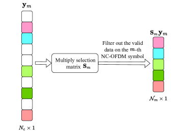
Figure 4: The process of selecting valid data. The various colored squares represent the different valid data, and the white squares represent the invalid data.

III-A2 Range estimation process

With the following four steps, we can use the unprocessed channel information matrix to estimate the target’s range information.

• Step 1: The processed channel information matrix is obtained by modulation symbol division and the spectrum occupancy sequence $\mathbf{A}_{m}$, e.g. (23).

• Step 2: For each non-zero column vector $\mathbf{y}_{m}$ of the processed channel information matrix, we use FISTA to solve (29) to obtain $\mathbf{P}_{m}$.

• Step 3: To improve anti-noise performance, we accumulate and normalize $M_{\text{a}}$ range power spectra, where $M_{\text{a}}\leq M_{\text{sym}}$ represents the number of non-zero column vectors $\mathbf{y}_{m}$. Given that the velocity of target is unknown, the accumulation is non-coherent.

• Step 4: The peak of power spectrum is searched to obtain the peak index value $k_{0}$, which is brought into (31) to get the range of target.

$$\hat{R}=\dfrac{c}{2N_{\text{c}}\Delta f}(k_{0}-1).$$ (31)

The improved range estimation algorithm is given in Algorithm 1.

In terms of target range estimation, the algorithm proposed in this paper is suitable for the scenario where the spectrum bands are dynamically changed and only the spectrum occupancy at each moment needs to be known. Therefore, this algorithm is highly adaptable.

Algorithm 1: Improved Range Estimation Algorithm
Input:	Unprocessed channel information matrix $\mathbf{D}_{\mathrm{R}}$; Spectrum occupancy sequence $\mathbf{A}_{m}$, $m\in\left\{{1,2,\cdots,M_{\text{sym}}}\right\}$; Selection matrix $\mathbf{S}_{m}$; The sensing matrix $\mathbf{J}_{m}$ for compressive reconstruction; Regularization parameter $\lambda$; The number of NC-OFDM symbols $M_{\text{sym}}$; The total number of subcarriers $N_{\text{c}}$;
1:	Initialize the processed channel information matrix $\mathbf{D^{\prime}}_{\mathrm{R}}\in\mathbb{C}^{N_{\text{c}}\times M_{\text{sym}}}$;
2:	For $\mathbf{D}_{\mathrm{R}}$ $m$ in $M_{\text{sym}}$ do
3:	The $m$-th column vector of $\mathbf{D}_{\mathrm{R}}$ and $\mathbf{A}_{m}$ perform the Hadamard product;
4:	Results of the 3 step $\to\mathbf{D^{\prime}}_{\mathrm{R}}(:,m)$;
5:	End For
6:	Obtain $\mathbf{D^{\prime}}_{\mathrm{R}}$;
7:	Initialize a range power spectrum $\mathbf{P}\in\mathbb{C}^{1\times N_{\text{c}}}$ and $i=1$;
8:	For $\mathbf{D^{\prime}}_{\mathrm{R}}$ $m$ in $M_{\text{sym}}$ do
9:	If the $m$-th column vector of $\mathbf{D^{\prime}}_{\mathrm{R}}$ $>0$ then
10:	Set the regularization parameter $\lambda$ according to Table 8 and 8;
11:	Set the maximum number of iterations $I_{\text{max}}$;
12:	Set the threshold of iterations error $\Theta$;
13:	The $m$-th column vector of $\mathbf{D^{\prime}}_{\mathrm{R}}$ and selection matrix $\mathbf{S}_{m}$ perform (30) to obtain $\mathcal{y^{\prime}}_{m}$;
14:	$\textbf{While}\ \text{error}(k+1)-\text{error}(k)\geq\Theta$ and $k\leq I_{\text{max}}$ do
15:	$(1)$ Take $\mathcal{P}_{1}=\mathcal{Z}\in\mathbb{R}^{N_{\text{c}}}$, $t_{1}=1$;
16:	$\cdots$
17:	$(k)$ $\mathcal{Z}_{k}=p_{L}(\mathcal{P}_{k})$ according to Table II;
18:	$t_{k+1}=\frac{1+\sqrt{1+4t_{k}^{2}}}{2}$;
19:	$\mathcal{P}_{k+1}=\mathcal{Z}_{k}+\left(\frac{t_{k}-1}{t_{k+1}}\right)(\mathcal{Z}_{k}-\mathcal{Z}_{k-1})$;
20:	$\text{error}(k+1)=\|\mathbf{J}_{m}\mathcal{Z}_{k}-\mathcal{y^{\prime}}_{m}\|_{2}$;
21:	End While
22:	Obtian the reconstruction data $\mathcal{Z}$;
23:	$\mathbf{P}=\mathbf{P}+|\mathcal{Z}|$, where $|\cdot|$ is an absolute value;
24:	$i=i+1$;
25:	End If
26:	End For
27:	$\mathbf{P}=\mathbf{P}/i$;
28:	Search for the peak value of $\mathbf{P}$ and get the peak index value;
29:	Substitute the index value into (31);
Output:	The range of target $\hat{R}$

III-B Velocity Estimation Algorithm

Since the Doppler effect causes a linear phase shift along the time axis, the target’s velocity can be obtained by processing row vectors of the channel information matrix. First, the processed channel information matrix need to be obtained. However, unlike the range estimation algorithm, $\mathbf{A}_{m}$ cannot be directly used for Hadamard product. Therefore the spectrum occupancy sequences in $M_{\text{sym}}$ symbol times need to be processed.

First, the matrix $\mathbf{Z}\in\mathbb{C}^{N_{\text{c}}\times M_{\text{sym}}}$ is obtained as follows by arranging the spectrum occupancy sequences $\mathbf{A}_{m}$ in $M_{\text{sym}}$ symbol times in rows.

$$\mathbf{Z}=\left(\mathbf{A}_{1},\mathbf{A}_{2},\cdots,\mathbf{A}_{m},\cdots,\mathbf{A}_{M_{\text{sym}}}\right).$$ (32)

Then, the $\mathbf{Z}$ is Hadamard product with the corresponding unprocessed channel information matrix to obtain the processed channel information matrix. The processed channel information matrix $\mathbf{D}_{\mathrm{V2}}$ under scenario 2 is expressed as (33),

$$\mathbf{D}_{\mathrm{V2}}=$$ (33)

$$\left[\begin{array}[]{cccccc}q_{1,1}+\varepsilon_{1,1}&\cdots&q_{1,\frac{M_{\text{sym}}}{2}}+\varepsilon_{1,\frac{M_{\text{sym}}}{2}}&0&\cdots&0\\ \vdots&\ddots&\vdots&\vdots&\ddots&\vdots\\ q_{\frac{\mathcal{N}_{m}}{2},1}+\varepsilon_{\frac{\mathcal{N}_{m}}{2},1}&\cdots&q_{\frac{\mathcal{N}_{m}}{2},\frac{M_{\text{sym}}}{2}}+\varepsilon_{\frac{\mathcal{N}_{m}}{2},\frac{M_{\text{sym}}}{2}}&0&\cdots&0\\ 0&\cdots&0&q_{\frac{\mathcal{N}_{m}}{2}+1,\frac{M_{\text{sym}}}{2}+1}+\varepsilon_{\frac{\mathcal{N}_{m}}{2}+1,\frac{M_{\text{sym}}}{2}+1}&\cdots&q_{\frac{\mathcal{N}_{m}}{2}+1,M_{\text{sym}}}+\varepsilon_{\frac{\mathcal{N}_{m}}{2}+1,M_{\text{sym}}}\\ \vdots&\ddots&\vdots&\vdots&\ddots&\vdots\\ 0&\cdots&0&q_{N_{\text{c}}-\frac{\mathcal{N}_{m}}{2},\frac{M_{\text{sym}}}{2}+1}+\varepsilon_{N_{\text{c}}-\frac{\mathcal{N}_{m}}{2},\frac{M_{\text{sym}}}{2}+1}&\cdots&q_{N_{\text{c}}-\frac{\mathcal{N}_{m}}{2},M_{\text{sym}}}+\varepsilon_{N_{\text{c}}-\frac{\mathcal{N}_{m}}{2},M_{\text{sym}}}\\ q_{N_{\text{c}}-\frac{\mathcal{N}_{m}}{2}+1,1}+\varepsilon_{N_{\text{c}}-\frac{\mathcal{N}_{m}}{2}+1,1}&\cdots&q_{N_{\text{c}}-\frac{\mathcal{N}_{m}}{2}+1,\frac{M_{\text{sym}}}{2}}+\varepsilon_{N_{\text{c}}-\frac{\mathcal{N}_{m}}{2}+1,\frac{M_{\text{sym}}}{2}}&0&\cdots&0\\ \vdots&\ddots&\vdots&\vdots&\ddots&\vdots\\ q_{N_{\text{c}},1}+\varepsilon_{N_{\text{c}},1}&\cdots&q_{N_{\text{c}},\frac{M_{\text{sym}}}{2}}+\varepsilon_{N_{\text{c}},\frac{M_{\text{sym}}}{2}}&0&\cdots&0\end{array}\right].$$

 

where $q_{m,n^{\prime}}$ represents that the data after the modulation symbols have undergone element-wise complex division.

III-B1 Compressive reconstruction of the power spectrum of velocity

The matrix $\mathbf{Z}$ is divided into $N_{\text{c}}$ row vectors and the $n^{\prime}$-th row vector is denoted by $\mathbf{U}_{n^{\prime}}$. The same operation is used for the matrix $\mathbf{D}_{\mathrm{V}2}$ to obtain the row vector $\mathbf{k}_{n^{\prime}}$ of its $n^{\prime}$-th row. The derivation of the equation is performed below, which is transformed into column vectors in order to be consistent with the derivation of the range estimation. Similar to (25), (26) and (27), we obtain the relationship in terms of velocity

$$(\mathbf{k}_{n^{\prime}})^{\mathrm{T}}=(\mathbf{U}_{n^{\prime}})^{\mathrm{T}}\circ(\mathbf{k}_{{n^{\prime}}(\text{full})})^{\mathrm{T}},$$ (34a)

$$\mathbf{k}_{{n^{\prime}}(\text{full})}\mathbf{\Upsilon}=\mathbf{Q}_{n^{\prime}},$$ (34b)

$$\mathbf{k}_{{n^{\prime}}(\text{full})}=\mathbf{Q}_{n^{\prime}}\mathbf{\Upsilon}^{-1},$$ (34c)

where $(\cdot)^{\mathrm{T}}$ represents transpose operation, $\mathbf{k}_{{n^{\prime}}(\text{full})}$ is the $n^{\prime}$-th row vector of the channel information matrix obtained from the OFDM signal that occupies all subcarriers, $\mathbf{\Upsilon}\in\mathbb{C}^{M_{\text{sym}}\times M_{\text{sym}}}$ is DFT matrix, and $\mathbf{Q}_{n^{\prime}}\in\mathbb{C}^{1\times M_{\text{sym}}}$ represents the power spectrum of velocity. Substituting (34c) into (34a), and expanding $\mathbf{U}_{n^{\prime}}$ into matrix $\mathbf{U^{\prime}}_{n^{\prime}}\in\mathbb{C}^{M_{\text{sym}}\times M_{\text{sym}}}$ for Hadamard product operation with $\mathbf{\Upsilon}$, we can get

$$(\mathbf{k}_{n^{\prime}})^{\mathrm{T}} =(\mathbf{U}_{n^{\prime}})^{\mathrm{T}}\circ(\mathbf{Q}_{n^{\prime}}\mathbf{\Upsilon}^{-1})^{\mathrm{T}}$$ (35)

$$=(\mathbf{U}_{n^{\prime}})^{\mathrm{T}}\circ\left[(\mathbf{\Upsilon}^{-1})^{\mathrm{T}}(\mathbf{Q}_{n^{\prime}})^{\mathrm{T}}\right]$$

$$=\left[(\mathbf{U^{\prime}}_{n^{\prime}})^{\mathrm{T}}\circ(\mathbf{\Upsilon}^{-1})^{\mathrm{T}}\right](\mathbf{Q}_{n^{\prime}})^{\mathrm{T}}$$

$$=\left(\mathbf{U^{\prime}}_{n^{\prime}}\circ\mathbf{\Upsilon}^{-1}\right)^{\mathrm{T}}(\mathbf{Q}_{n^{\prime}})^{\mathrm{T}},$$

where $\mathbf{U^{\prime}}_{n^{\prime}}=\left(\mathbf{U}_{n^{\prime}},\mathbf{U}_{n^{\prime}},\cdots,\mathbf{U}_{n^{\prime}}\right)^{\mathrm{T}}$. Define a selection matrix $\mathbf{G}_{n^{\prime}}\in\mathbb{C}^{\mathcal{M}_{n^{\prime}}\times M_{\text{sym}}}$ to filter out the valid data on the $n^{\prime}$-th subcarrier. $\mathcal{M}_{n^{\prime}}$ is the number of valid data in the $n^{\prime}$-th subcarrier and the intuitive filtering process is similar to Fig. 4. Multiplying both sides of (35) by $\mathbf{G}_{n^{\prime}}$, we have

$$\mathbf{k^{\prime}}_{n^{\prime}}=\mathbf{F}_{n^{\prime}}(\mathbf{Q}_{n^{\prime}})^{\mathrm{T}},$$ (36)

where

$$\begin{cases}\mathbf{k^{\prime}}_{n^{\prime}}=\mathbf{G}_{n^{\prime}}(\mathbf{k}_{n^{\prime}})^{\mathrm{T}}\\ \mathbf{F}_{n^{\prime}}\in\mathbb{C}^{\mathcal{M}_{n^{\prime}}\times M_{\text{sym}}}=\mathbf{G}_{n^{\prime}}\left(\mathbf{U^{\prime}}_{n^{\prime}}\circ\mathbf{\Upsilon}^{-1}\right)^{\mathrm{T}}\end{cases}$$ (37)

Since the sensing matrix $\mathbf{F}_{n^{\prime}}$ is a partial IDFT matrix and $(\mathbf{k}_{n^{\prime}})^{\mathrm{T}}$ is a sparse vector, the conditions for accurate reconstruction of the spare vector $\mathbf{Q}_{n^{\prime}}$ are still satisfied. The FISTA is applied to solve the optimization problem.

III-B2 Velocity estimation process

With the following four steps, we can use the unprocessed channel information matrix to estimate the target’s velocity information.

• Step 1: The processed channel information matrix is obtained by an element-wise complex division and the matrix $\mathbf{Z}$, e.g. (33).

• Step 2: For each non-zero row vector $\mathbf{k}_{n}$ of the processed channel information matrix, the FISTA is applied to obtain $\mathbf{Q}_{n^{\prime}}$.

• Step 3: To improve anti-noise performance, we accumulate and normalize $N_{\text{b}}$ number of $\mathbf{Q}_{n^{\prime}}$. $N_{\text{b}}\leq N_{\text{c}}$ is the number of non-zero row vectors $\mathbf{k}_{n^{\prime}}$. Given that the range of target is unknown, the accumulation is non-coherent.

• Step 4: The peak of power spectrum is searched to obtain the peak index value $l_{0}$, which is substituted into (38) to get the velocity of target.

$$\hat{v_{0}}=\frac{c}{2M_{\text{sym}}T_{\text{sym}}f_{\text{c}}}(l_{0}-1).$$ (38)

The improved velocity estimation algorithm is given in Algorithm 2.

Algorithm 2: Improved Velocity Estimation Algorithm
Input:	Unprocessed channel information matrix $\mathbf{D}_{\mathrm{R}}$; Spectrum occupancy sequence $\mathbf{A}_{m}$,$m\in{1,2,\cdots,M_{\text{sym}}}$; Selection matrix $\mathbf{G}_{n^{\prime}}$; The sensing matrix $\mathbf{F}_{n^{\prime}}$ for compressive reconstruction; Regularization parameter $\lambda$; The number of NC-OFDM symbols $M_{\text{sym}}$; The total number of subcarriers $N_{\text{c}}$;
1:	Initialize a matrix $\mathbf{Z}\in\mathbb{C}^{N_{\text{c}}\times M_{\text{sym}}}$;
2:	For $\mathbf{Z}$ $m$ in $M_{\text{sym}}$ do
3:	The $m$-th sequence $\mathbf{A}_{m}$ $\to\mathbf{Z}(:,m)$;
4:	End For
5:	Obtain $\mathbf{Z}$;
6:	Initialize the processed channel information matrix $\mathbf{D^{\prime}}_{\mathrm{V}}\in\mathbb{C}^{N_{\text{c}}\times M_{\text{sym}}}$;
7:	The matrix $\mathbf{D}_{\mathrm{V}}$ and matrix $\mathbf{Z}$ perform the Hadamard product $\to\mathbf{D^{\prime}}_{\mathrm{V}}(:,:)$;
8:	Obtain $\mathbf{D^{\prime}}_{\mathrm{V}}$;
9:	Initialize a velocity power spectrum $\mathbf{Q}\in\mathbb{C}^{1\times M_{\text{sym}}}$ and $i=1$;
10:	For $\mathbf{D^{\prime}}_{\mathrm{V}}$ $n^{\prime}$ in $N_{\text{c}}$ do
11:	If the $n^{\prime}$-th row vector of $\mathbf{D^{\prime}}_{\mathrm{V}}$ $>0$ then
12:	Set the regularization parameter $\lambda$ according to Table 8 and Table 8;
13:	Set the maximum number of iterations $I_{\text{max}}$;
14:	Set the threshold of iterations error $\Theta$;
15:	The $n^{\prime}$-th row vector of $\mathbf{D^{\prime}}_{\mathrm{V}}$ and the selection matrix $\mathbf{G_{n^{\prime}}}$ perform (37) to obtain $\mathcal{K^{\prime}}_{n^{\prime}}$;
16:	$\textbf{While}\ \text{error}(k+1)-\text{error}(k)\geq\Theta$ and $k\leq I_{\text{max}}$ do
17:	$(1)$ Take $\mathcal{P}_{1}=\mathcal{Z}\in\mathbb{R}^{M_{\text{sym}}}$, $t=1$;
18:	$\cdots$
19:	$(k)$ $\mathcal{Z}_{k}=p_{L}(\mathcal{P}_{k})$;
20:	$t_{k+1}=\frac{1+\sqrt{1+4t_{k}^{2}}}{2}$;
21:	$\mathcal{P}_{k+1}=\mathcal{Z}_{k}+\left(\frac{t_{k}-1}{t_{k+1}}\right)(\mathcal{Z}_{k}-\mathcal{Z}_{k-1})$;
22:	$\text{error}(k+1)=\|\mathbf{F}_{n^{\prime}}\mathcal{Z}_{k}-\mathcal{K^{\prime}}_{n^{\prime}}\|_{2}$;
23:	End While
24:	Obtain the reconstruction data $\mathcal{Z}$;
25:	$\mathbf{Q}=\mathbf{Q}+|(\mathcal{Z})^{\text{T}}|$;
26:	$i=i+1$;
27:	End If
28:	End For
29:	$\mathbf{Q}=\mathbf{Q}/i$;
30:	Search for the peak value of $\mathbf{Q}$ and get the peak index value;
31:	Substitute the index value into $(\ref{eq28})$;
Output:	The velocity of target $\hat{v_{0}}$

When the input $\mathbf{y}_{m}$ or $\mathbf{k}_{n^{\prime}}$ is a vector without zero elements, such as the first row vector under scenario 1. In this case, there is no deterioration of sidelobes due to the zero elements. However, using the FISTA can achieve the effect of noise reduction, and the noise reduction can also improve PSR [28].

IV The Selection of $\lambda$ based on Machine Learning and Sensing Performance Analysis

In this section, the KCV in machine learning is applied to find the optimal value of $\lambda$, which results in a faster and more accurate reconstruction capability for JCMSA. Then, the impact of JCMSA on sensing performance including SNR gain and resolution is analyzed.

IV-A The Selection of $\lambda$ based on Machine Learning

FISTA is a fast algorithm used to solve linear inverse problems and can also be applied to CS reconstruction problems. For the mathematical model of the solution of (7), it can be transformed into an equivalent mathematical model [29]

$$\min\limits_{\theta}\frac{1}{2}\|\mathbf{A}\theta-\mathbf{y}\|_{2}^{2}+\lambda\|\theta\|_{1},$$ (39)

where $\|\cdot\|_{2}$ represents the $\ell_{2}$-norm, and $\lambda$ is the regularization parameter [15]. This is a least square optimization problem with an $\ell_{1}$ regularization term. The FISTA used for solving such problems are shown in Table II.

TABLE II: FISTA with a constant stepsize [15].

Input: $L=L(f)$ : A Lipschitz constant of $\bigtriangledown f$.

Step 0. Take $\mathbf{y}_{1}=\mathbf{x}_{0}\in\mathbb{R}^{n}$, $t_{1}=1$.

Step k. $(k\geq 1)$ Compute

$\mathrm{x}_{k}=p_{L}(\mathbf{y}_{k})$,

$t_{k+1}=\frac{1+\sqrt{1+4{t_{k}}^{2}}}{2}$,

$\mathbf{y}_{k+1}=\mathbf{x}_{k}+(\frac{t_{k}-1}{t_{k+1}})(\mathbf{x}_{k}-\mathbf{x}_{k-1})$,

where

$p_{L}(\mathbf{y})=\underset{\mathbf{x}}{\operatorname*{argmin}}\left\{g(\mathbf{x})+\frac{L}{2}\left\|\mathbf{x}-\left(\mathbf{y}-\frac{1}{L}\nabla f(\mathbf{y})\right)\right\|^{2}\right\}$,

$g(\mathbf{x})=\lambda\|\mathbf{x}\|_{1}$ ,

Since the $\lambda$ effects overfitting and underfitting, choosing the appropriate regularisation parameter is beneficial to obtain the optimal reconstruction. The selection of the optimal $\lambda$ in machine learning applications is achieved using the KCV technique [30].

In KCV, the dataset is divided into $\mathbf{K}$ folds, a model is learned using $\mathbf{K}-1$ folds, and an error value is calculated by testing the model in the remaining fold. Finally, the KCV estimation of the error is the average value of the errors committed in each fold [31]. In this paper, the training set is not used for training as the mathematical model is already given, e.g. (39). We reconstruct the test set using the FISTA in each iteration and use the reconstruction error and the speed of convergence as scores to select the optimal $\lambda$.

• Dataset selection: For the input dataset, we use the processed channel information matrix as the observation dataset, e.g. (23). The sparse power spectrum is also used as the ideal reconstruction dataset and the sensing matrix is used as the sensing matrix dataset, e.g. $\mathbf{J}_{m}$ or $\mathbf{F}_{n^{\prime}}$.

• Trade-offs for rewards: We use reconstruction error and convergence speed as a bonus (or score), both of which are $90$ percent and $10$ percent, respectively. The goal is to find the optimal $\lambda$ for different SNRs within an interval of $\lambda$ using grid searches of different step sizes.

A detailed flow chart for the selection of $\lambda$ is shown in Fig. 5.

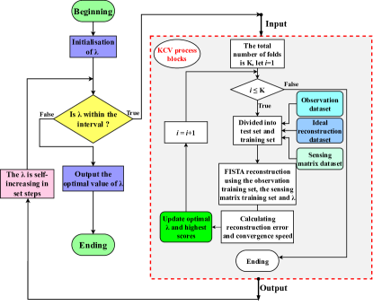
Figure 5: The flow chart for the selection of $\lambda$.

IV-B Sensing Performance Analysis

IV-B1 SNR performance

An important performance metric is the SNR of radar estimation. We take the channel information matrix in scenario 1 as the scenario of SNR performance analysis, and the channel information matrix in other scenarios can be analyzed in the same way using the following procedures.

The SNR gain with JCMSA processing has three contributions: the gain generated by DFT or IDFT processing, the gain generated by FISTA processing, and the gain generated by non-coherent accumulation. Given that the gain from FISTA processing is related to the regularisation parameter and the Lipschitz constant [15], which is adjusted according to the optimization model and the practical SNR situation. We assume that the gain produced by FISTA processing is $\varpi\ (\varpi\geq 0)$.

The assumptions for performance analysis are as follows.

1. SNR is defined as (40), where $P_{\text{s}}(x)$ and $P_{\text{noise}}$ denote the power of signal and noise, respectively. $N$ is the number of sampling points of $x$ in $P_{\text{s}}(x)$.

2. In scenario 1, a total of $\mathcal{N}_{m}\ (\mathcal{N}_{m}<N_{\text{c}})$ subcarriers are available. Consider $\hat{\textbf{D}}_{\mathrm{R1}}$ as the matrix of unprocessed channel information under scenario 1, and the element $K_{m,n^{\prime}}$ in $\hat{\textbf{D}}_{\mathrm{R1}}$ is written as (41), where $K^{\prime}_{m,n^{\prime}}$ and $\varepsilon_{m,n^{\prime}}$ are the signal and noise component in $K_{m,n^{\prime}}$, respectively.

3. Suppose that the modulus of $K^{\prime}_{m,n^{\prime}}$ in each element of matrix $\hat{\textbf{D}}_{\mathrm{R1}}$ is $h$, while the variance of noise component $\varepsilon_{m,n^{\prime}}$ is $h^{2}\sigma^{2}$.

$$\begin{cases}\text{SNR}=\dfrac{P_{\text{s}}(x)}{P_{\text{noise}}},\\[7.0pt] P_{\text{s}}(x)=\dfrac{\sum_{\mu=0}^{N-1}\left|x(\mu)\right|^{2}}{N},\\[7.0pt] x\ $is the discrete signal sequence.$\end{cases}$$ (40)

$$K_{m,n^{\prime}}=\begin{cases}\varepsilon_{m,n^{\prime}},K_{m,n^{\prime}}$\ in licensed point$,\\ K^{\prime}_{m,n^{\prime}}+\varepsilon_{m,n^{\prime}},K_{m,n^{\prime}}$\ in unlicensed point $.\end{cases}$$ (41)

Theorem 1

When FISTA finds the optimal parameter $\lambda$, the SNR gain with FISTA is $\varpi>0$, and hence we derive

$$\begin{cases}\underbrace{\sqrt{M_{\text{sym}}}\left(\frac{\mathcal{N}_{m}}{\sigma^{2}}+\varpi\right)}_{\text{ JCMSA}}>\underbrace{\frac{\sqrt{M_{\text{sym}}}\mathcal{N}_{m}}{\sigma^{2}}}_{\text{ \cite[cite]{[\@@bibref{}{wei2022robust}{}{}]}}}>\underbrace{\frac{\mathcal{N}_{m}^{2}}{N_{\text{c}}\sigma^{2}}}_{\text{2D FFT}},\ (\mathrm{range})\\ \underbrace{\sqrt{\mathcal{N}_{m}}\left(\frac{M_{\text{sym}}}{\sigma^{2}}+\varpi\right)}_{\text{ JCMSA}}>\underbrace{\frac{\sqrt{\mathcal{N}_{m}}M_{\text{sym}}}{\sigma^{2}}}_{\text{ \cite[cite]{[\@@bibref{}{wei2022robust}{}{}]}}}>\underbrace{\frac{M_{\text{sym}}}{\sigma^{2}}}_{\text{2D FFT}}.\ (\mathrm{velocity})\end{cases}$$ (42)

Proof:

In the following, we first derive the SNR gains for range and velocity with JCMSA processing, and then give the SNR gains with conventional 2D FFT processing and the SNR gains with improved algorithm processing in [14]. The results show that the JCMSA proposed in this paper has better SNR performance gain.

The SNR gain of range with JCMSA processing is derived as follows.

• Step 1: After the lines 1-6 in Algorithm 1, each column vector of matrix $\hat{\textbf{D}}_{\mathrm{R1}}$ contains $\mathcal{N}_{m}$ signal elements and $\mathcal{N}_{m}$ noise elements.

• Step 2: The lines 7-26 in Algorithm 1 contains three operations: IDFT, FISTA, and non-coherent accumulation. After the IDFT on each column vector, the SNR of each column vector is $\mathcal{N}_{m}/\sigma^{2}$. Then after FISTA, the SNR is improved to $(\mathcal{N}_{m}/\sigma^{2})+\varpi$.

• Step 3: It is not possible to directly compute an SNR after non-coherent accumulation from [32]. Therefore, in this paper, the non-coherent accumulation gain is assumed to be $\sqrt{E}$, where $E$ is the number of symbols undergoing non-coherent accumulation. In scenario 1, there are $M_{\text{sym}}$ symbols for non-coherent accumulation. Thus, after the non-coherent accumulation, the SNR of output signal is $\sqrt{M_{\text{sym}}}\left[(\mathcal{N}_{m}/\sigma^{2})+\varpi\right]$.

The SNR gain of velocity with JCMSA processing is derived as follows.

• Step 1: After the lines 1-8 in Algorithm 2, the noise elements of the unavailable subcarrier positions in $\hat{\textbf{D}}_{\mathrm{R1}}$ are zeroed out.

• Step 2: The lines 9-28 in Algorithm 2 contains three operations: DFT, FISTA, and non-coherent accumulation. After the DFT on each row vector, the SNR of each row vector is $M_{\text{sym}}/\sigma^{2}$. Then after FISTA, the SNR is improved to $(M_{\text{sym}}/\sigma^{2})+\varpi$.

• Step 3: Unlike the non-coherent accumulation of range, the number of accumulations is the number of available subcarriers, i.e., $\mathcal{N}_{m}$. Thus, after the non-coherent accumulation, the SNR of output signal is $\sqrt{\mathcal{N}_{m}}\left[(M_{\text{sym}}/\sigma^{2})+\varpi\right]$.

For the conventional 2D FFT algorithm, IDFT is performed on a column of $\hat{\textbf{D}}_{\mathrm{R1}}$ to obtain the range power spectrum, and DFT is performed on a row to obtain the velocity power spectrum. Thus, the SNR for range and velocity of the output signal after the conventional 2D FFT algorithm are $\mathcal{N}_{m}^{2}/(N_{\text{c}}\sigma^{2})$ and $M_{\text{sym}}/\sigma^{2}$, respectively.

For the improved algorithm in [14], only the FISTA gain is missing compared to JCMSA. Hence, the total SNR gain results are just missing $\varpi$. ∎

Theorem 2

When the input signal-to-noise ratio lower than -25 dB, it is difficult to find the optimal FISTA parameter $\lambda$, i.e. $\varpi\approx 0$. Thus, we derive

$$\begin{cases}\underbrace{\sqrt{M_{\text{sym}}}\left(\frac{\mathcal{N}_{m}}{\sigma^{2}}\right)}_{\text{ JCMSA}}\approx\underbrace{\frac{\sqrt{M_{\text{sym}}}\mathcal{N}_{m}}{\sigma^{2}}}_{\text{ \cite[cite]{[\@@bibref{}{wei2022robust}{}{}]}}}>\underbrace{\frac{\mathcal{N}_{m}^{2}}{N_{\text{c}}\sigma^{2}}}_{\text{2D FFT}},\ (\mathrm{range})\\ \underbrace{\sqrt{\mathcal{N}_{m}}\left(\frac{M_{\text{sym}}}{\sigma^{2}}\right)}_{\text{ JCMSA}}\approx\underbrace{\frac{\sqrt{\mathcal{N}_{m}}M_{\text{sym}}}{\sigma^{2}}}_{\text{ \cite[cite]{[\@@bibref{}{wei2022robust}{}{}]}}}>\underbrace{\frac{M_{\text{sym}}}{\sigma^{2}}}_{\text{2D FFT}}.\ (\mathrm{velocity})\end{cases}$$ (43)

Proof:

Upon observing the (42) in Theorem 1, we notice that the only difference between the SNR gains of JCMSA and improved algorithm in [14] is $\varpi$. Therefore, When $\varpi\approx 0$, the JCMSA and improved algorithm in [14] have similar SNR gains, both of which perform better than the conventional 2D FFT algorithm. ∎

IV-B2 Resolution performance

As depicted in Fig. 6, two extreme cases of spectrum occupancy have been selected to facilitate the analysis of resolution.

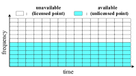
(a) Continuous occupancy of $N_{\text{c}}/2$ subcarriers within a sensing frame.

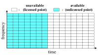
(b) Continuous occupancy of $M_{\text{sym}}/2$ NC-OFDM symbols within a sensing frame.

Figure 6: Dynamic changes in spectrum occupancy.

For conventional 2D FFT algorithm, the resolution of the range is not affected by the waveform used or the specific parameterization of the NC-OFDM system. It is solely determined by the bandwidth taken up by the transmit signal[33]. Therefore, When the spectrum occupancy of the ISAC system is as shown in Fig. 6(a), the range resolution of the conventional 2D FFT algorithm is

$$\Delta R=\frac{c}{\Delta f\times N_{\text{c}}}\ (\text{2D FFT algorithm}).$$ (44)

Given that the velocity resolution is related to the total duration of the sensing symbols. Therefore, When the spectrum occupancy of the ISAC system as shown in Fig. 6(b), the velocity resolution of the conventional 2D FFT algorithm is

$$\Delta v=\frac{c}{T_{\text{sym}}f_{\text{c}}M_{\text{sym}}}\ (\text{2D FFT algorithm}).$$ (45)

In the JCMSA-enabled ISAC system working in unlicensed spectrum bands, the sensing performance under full bandwidth or full sensing symbols can be obtained, thereby maintaining the maximum resolution, e.g.,(46).

$$\text{JCMSA}\begin{cases}\Delta R=\dfrac{c}{2\Delta fN_{\text{c}}},\\ \Delta v=\dfrac{c}{2T_{\text{sym}}f_{\text{c}}M_{\text{sym}}}.\end{cases}$$ (46)

TABLE III: Simulation parameters

Symbol	Parameter	Value
$N_{\text{c}}$	Number of subcarriers	$512$
$\mathcal{N}_{m}$	Number of occupied subcarriers	$256$
$M_{\text{sym}}$	Number of symbols	$14$
$f_{\text{c}}$	Carrier frequency	24 GHz
$\Delta f$	Subcarrier spacing	15 KHz
$T_{\text{ofdm}}$	Elementary NC-OFDM symbol duration	66.67 $\mu m$
$T_{\text{cp}}$	Cyclic prefix length	16.67 $\mu m$
$T_{\text{sym}}$	Entire NC-OFDM symbol duration	83.34 $\mu m$
$R$	Range of the target	117 $m$
$v$	Velocity of the target	13 $m/s$
K	Number of folds in KCV	14

V Simulation Results and Analysis

In this section, NC-OFDM ISAC signal is applied to sense a surrounding target with a relative velocity of $13$ m/s and a relative range of $117$ m. The simulation parameters are shown in Table III. In order to show the performance improvement of the JCMSA proposed in this paper, we evaluate the performance of the parameter estimation of target in terms of both power spectrum and root mean square error (RMSE), respectively, and compare the JCMSA with the improved algorithm in [14] and the conventional 2D FFT algorithm.

In the simulation, the optimal regularization parameter $\lambda$ for different SNRs is obtained by $14$-fold KCV. Table 8 and Table 8 show the optimal parameters of range and velocity estimation for different spectrum occupancy scenarios, respectively. Simulation results for the power spectra and RMSE are revealed as follows.

Figure 7: Optimal $\lambda$ for target estimation under scenario 1. The step size of $\lambda$ for range estimation is 100 and the interval is [1, 10000]. The step size of $\lambda$ for velocity estimation is 0.02 and the interval is [1, 5].

Range estimation under scenario 1
SNR (dB)	0	1	2	3	4	5	6	7	8	9	10
optimal $\lambda$	5401	5601	5001	4601	5401	5201	5001	5601	5601	5601	5201
Velocity estimation under scenario 1
SNR (dB)	0	1	2	3	4	5	6	7	8	9	10
optimal $\lambda$	2.16	1.56	1.54	1.08	1.2	1.12	0.74	0.68	1.16	1.7	1.5

Figure 8: Optimal $\lambda$ for target under scenario 2. The step size of $\lambda$ for range is 100 and the interval is [1, 10000]. The step size of $\lambda$ for velocity is 0.02 and the interval is [1, 5].

Range estimation under scenario 2
SNR (dB)	0	1	2	3	4	5	6	7	8	9	10
optimal $\lambda$	2501	3501	4501	3001	5001	4001	4801	5101	5201	5601	5101
Velocity estimation under scenario 2
SNR (dB)	0	1	2	3	4	5	6	7	8	9	10
optimal $\lambda$	1.32	1.70	1.44	1.28	0.92	1.20	1.10	1.46	1.70	1.56	1.54

 

V-A Power Spectra

In this subsection, we use the parameters in Table III in simulation, revealing the range and velocity power spectra for two scenarios.

Fig. 9 and Fig. 10 show the results of the power spectra for scenario 1 and scenario 2 respectively. The simulation results show that the peak index value of the range power spectrum is $\text{ind}_{r}=7$ and the peak index value of the velocity power spectrum is $\text{ind}_{v}=3$. The estimated range of the target is 117.1875 m and the estimated velocity is 13.3929 m/s when substituted into (31) and (38), respectively. Meanwhile, it is revealed from Fig. 9(a), Fig. 10(a), and Fig. 10(b) that the cavity caused by the spectral discontinuity worsens the power spectral sidelobes, and the improved 2D FFT algorithm in [14] cannot solve this problem, while the JCMSA proposed in this paper can always maintain zero sidelobes. For the case shown in Fig. 9(b), the sidelobe deterioration does not occur as there are no spectrum holes when velocity estimation is performed. However, the JCMSA proposed in this paper is able to perform a denoising effect and improve the PSR to a greater level.

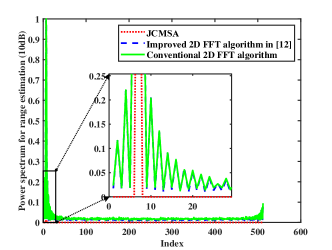
(a) Range estimate at SNR of 10 dB.

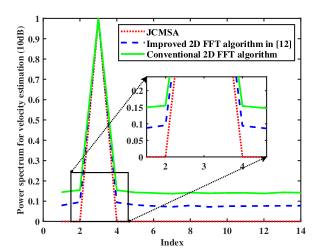
(b) Velocity estimate at SNR of 10 dB.

Figure 9: Power spectrum under scenario 1.

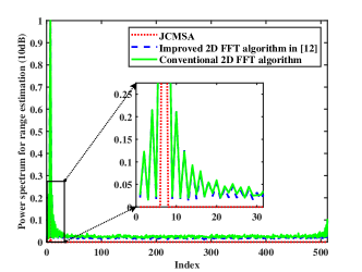
(a) Range estimate at SNR of 10 dB.

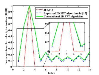
(b) Velocity estimate at SNR of 10 dB.

Figure 10: Power spectrum under scenario 2.

V-B RMSE

RMSE is the parameter used to reveal the error between the estimated value and the real value. With the same simulation parameters, this subsection compares the RMSE of range and velocity estimation under the three algorithms above. In this simulation, there exist theoretical upper and lower bounds for the RMSE of range and velocity due to the influence of spectrum resources and algorithms. According to the simulation parameters, (31), and (38), the upper and lower bounds are obtained as follows.

$$\overbrace{\textbf{RMSE-R}}^{\rm{upper\ bound}}=\dfrac{c(N_{\text{c}}-1)}{2N_{\text{c}}\Delta f}-117=0.9863\times 10^{4}\ \text{m},$$ (47a)

$$\underbrace{\textbf{RMSE-R}}_{\rm{lower\ bound}}=\dfrac{c(\text{ind}_{n}-1)}{2N_{\text{c}}\Delta f}-117=0.1875\ \text{m},$$ (47b)

$$\overbrace{\textbf{RMSE-V}}^{\rm{upper\ bound}}=\dfrac{c(M_{\text{sym}}-1)}{2M_{\text{sym}}T_{\text{sym}}f_{\text{c}}}-13=56.56\ \text{m/s},$$ (48a)

$$\underbrace{\textbf{RMSE-V}}_{\rm{lower\ bound}}=\dfrac{c(\text{ind}_{m}-1)}{2M_{\text{sym}}T_{\text{sym}}f_{\text{c}}}-13=0.3929\ \text{m/s}.$$ (48b)

Fig. 11 and Fig. 12 show the results of the RMSEs of range and velocity estimations under scenario 1 and scenario 2, respectively. According to the simulation results, three conclusions are drawn as follows.

1. The JCMSA and the improved algorithm in [14] have similar anti-noise performance. The anti-noise performance and SNR gain are correlated. When the input SNR is low, the JCMSA and improved algorithm in [14] have similar SNR gains, which is proved in Theorem 2. Thus, both algorithms show similar anti-noise performance when the SNR is less than $-10$ dB.

2. The JCMSA has better anti-noise performance than conventional 2D FFT algorithms, because the SNR is larger than conventional 2D FFT with JCMSA, which is proved in Theorem 1 and Theorem 2.

3. When the SNR is below $-25$ dB, the estimated RMSE error is mainly affected by noise, so that the average error of the RMSE hardly reach the theoretical upper bound ((47a), (48a)). When the SNR is higher than a certain value, the estimated RMSE depends on the resolution. The theoretical lower bound of the RMSE is also determined by the resolution, so that the estimated RMSE can reach the theoretical lower bound ((47b), (48b)).

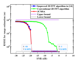
(a) RMSE for range estimation.

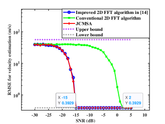
(b) RMSE for velocity estimation.

Figure 11: RMSE under scenario 1.

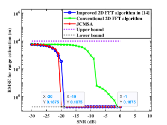
(a) RMSE for range estimation.

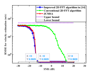
(b) RMSE for velocity estimation.

Figure 12: RMSE under scenario 2.

VI Conclution

For the ISAC-enabled mobile communication systems operating in unlicensed spectrum bands, conventional radar signal processing algorithms suffer from sidelobes deterioration and low anti-noise performance. To this end, the “Joint CS and Machine Learning ISAC Signal Processing Algorithm” is proposed in this paper, which can solve the problem of sidelobes deterioration and enhance anti-noise performance. More specifically, combining the RBG configuration information in 5G NR and CS techniques, which exploit the sparsity of the target to reconstruct the complete radar map, the enhanced range and velocity estimation algorithms are proposed. Then, the FISTA algorithm is used to solve the convex optimization problem, while KCV is employed to select the regularization parameter to obtain zero sidelobes and better anti-noise performance than conventional 2D FFT algorithm. With the emergence of numerous services, unlicensed spectrum bands have a large probability to be applied in in ISAC-enabled mobile communication systems. The work of this paper may provide beneficial references for the sensing algorithm design of the ISAC systems over unlicensed spectrum bands.

References

- [1] L. Fan, Y. Weijie, Y. Jinhong, Z. J. Andrew, F. Zesong, and Z. Jianming, “Radar-communication spectrum sharing and integration: Overview and prospect,” Journal of Radars, vol. 10, no. 3, pp. 467–484, 2021.
- [2] Z. Feng, Z. Fang, Z. Wei, X. Chen, Z. Quan, and D. Ji, “Joint radar and communication: A survey,” China Communications, vol. 17, no. 1, pp. 1–27, Jan 2020.
- [3] J. Mitola, “Cognitive radio for flexible mobile multimedia communications,” in 1999 IEEE International Workshop on Mobile Multimedia Communications (MoMuC’99)(Cat. No. 99EX384). IEEE, Nov 1999, pp. 3–10.
- [4] Z. Yao, W. Cheng, and H. Zhang, “Full-duplex assisted LTE-U/Wifi coexisting networks in unlicensed spectrum,” IEEE Access, vol. 6, pp. 40 085–40 095, Jul 2018.
- [5] X. Chen, “Research on Vehicle-mounted Radar Range and Velocity Measurement Method Based on OFDM Pilot signal,” Master’s thesis, Hunan University, 2015.
- [6] D. Bao, G. Qin, and Y.-Y. Dong, “A superimposed pilot-based integrated radar and communication system,” IEEE Access, vol. 8, pp. 11 520–11 533, Jan 2020.
- [7] F. LIU, Y. LIU, A. LI, C. Masouros, and Y. Eldar, “Cramér-rao bound optimization for joint radar-communication design,” arXiv preprint arXiv:2101.12530, 2021.
- [8] E. Tzoreff and A. J. Weiss, “Single Sensor Path Design for Best Emitter Localization via Convex Optimization,” IEEE Transactions on Wireless Communications, vol. 16, no. 2, pp. 939–951, Feb 2017.
- [9] Z. Huang, K. Wang, A. Liu, Y. Cai, R. Du, and T. X. Han, “Joint Pilot Optimization, Target Detection and Channel Estimation for Integrated Sensing and Communication Systems,” IEEE Transactions on Wireless Communications, vol. 21, no. 12, pp. 10 351–10 365, Dec 2022.
- [10] B. Schweizer, C. Knill, D. Schindler, and C. Waldschmidt, “Stepped-carrier OFDM-radar processing scheme to retrieve high-resolution range-velocity profile at low sampling rate,” IEEE Transactions on Microwave Theory and Techniques, vol. 66, no. 3, pp. 1610–1618, Sep 2017.
- [11] C. Knill, B. Schweizer, S. Sparrer, F. Roos, R. F. Fischer, and C. Waldschmidt, “High range and Doppler resolution by application of compressed sensing using low baseband bandwidth OFDM radar,” IEEE Transactions on Microwave Theory and Techniques, vol. 66, no. 7, pp. 3535–3546, Jun 2018.
- [12] C. Sturm, Y. L. Sit, M. Braun, and T. Zwick, “Spectrally interleaved multi-carrier signals for radar network applications and multi-input multi-output radar,” IET Radar, Sonar & Navigation, vol. 7, no. 3, pp. 261–269, Mar 2013.
- [13] G. Hakobyan and B. Yang, “A novel OFDM-MIMO radar with non-equidistant dynamic subcarrier interleaving,” in 2016 European Radar Conference (EuRAD). IEEE, Oct 2016, pp. 45–48.
- [14] Z. Wei, H. Qu, L. Ma, and C. Pan, “Robust ISAC Signal Processing on Unlicensed Spectrum Bands,” in 2022 IEEE/CIC International Conference on Communications in China (ICCC Workshops). IEEE, Aug 2022, pp. 117–121.
- [15] A. Beck and M. Teboulle, “A fast iterative shrinkage-thresholding algorithm for linear inverse problems,” SIAM journal on imaging sciences, vol. 2, no. 1, pp. 183–202, 2009.
- [16] C. Sturm and W. Wiesbeck, “Waveform Design and Signal Processing Aspects for Fusion of Wireless Communications and Radar Sensing,” Proceedings of the IEEE, vol. 99, no. 7, pp. 1236–1259, Jul 2011.
- [17] Y. Huang, D. Huang, Q. Luo, S. Ma, S. Hu, and Y. Gao, “NC-OFDM RadCom system for electromagnetic spectrum interference,” in 2017 IEEE 17th International Conference on Communication Technology (ICCT). IEEE, Oct 2017, pp. 877–881.
- [18] F. Liu, Y. Cui, C. Masouros, J. Xu, T. X. Han, Y. C. Eldar, and S. Buzzi, “Integrated Sensing and Communications: Toward Dual-Functional Wireless Networks for 6G and Beyond,” IEEE Journal on Selected Areas in Communications, vol. 40, no. 6, pp. 1728–1767, Jun 2022.
- [19] J. Thomas and P. P. Menon, “A survey on spectrum handoff in cognitive radio networks,” in 2017 International Conference on Innovations in Information, Embedded and Communication Systems (ICIIECS), Mar 2017, pp. 1–4.
- [20] Y. Liu, “Research on cognitive radio technology based on compressed sensing,” Master’s thesis, Xidian University, 2015.
- [21] X.-Y. He, R.-F. Song, and K.-Q. Zhou, “Compressive sensing based channel estimation for NC-OFDM systems in cognitive radio context,” Journal of China Institute of Communications, vol. 32, no. 11, pp. 85–94, Nov 2011.
- [22] D. S. Hochba, “Approximation algorithms for NP-hard problems,” ACM Sigact News, vol. 28, no. 2, pp. 40–52, Jun 1997.
- [23] E. J. Candès and M. B. Wakin, “An introduction to compressive sampling,” IEEE signal processing magazine, vol. 25, no. 2, pp. 21–30, Mar 2008.
- [24] G. Taubock and F. Hlawatsch, “A compressed sensing technique for OFDM channel estimation in mobile environments: Exploiting channel sparsity for reducing pilots,” in 2008 IEEE International Conference on Acoustics, Speech and Signal Processing. IEEE, Apr 2008, pp. 2885–2888.
- [25] G. Huang, “Research on modulation techniques for fusion of radar and communications,” Ph.D. dissertation, Guilin University Of Electronic Technology, 2021.
- [26] G. Huang, S. Ouyang, and K. Liao, “Review on Signal Modulation Techniques for Joint Radar-Communication Systems,” Radio Engineering, vol. 52, no. 336-349, Mar 2022.
- [27] E. J. Candes and T. Tao, “Near-optimal signal recovery from random projections: Universal encoding strategies?” IEEE transactions on information theory, vol. 52, no. 12, pp. 5406–5425, Dec 2006.
- [28] X. Wu, K. Lu, H. Liang, and J. Xue, “Enhancing the Image Resolution of Acoustic Microscopy with FISTA,” in 2021 5th International Conference on Automation, Control and Robots (ICACR), Sep 2021, pp. 7–11.
- [29] G. Kutyniok, “Theory and applications of compressed sensing,” GAMM-Mitteilungen, vol. 36, no. 1, pp. 79–101, Aug 2013.
- [30] Z. Han, H. Li, and W. Yin, Compressive sensing for wireless networks. Cambridge University Press, 2013.
- [31] J. D. Rodriguez, A. Perez, and J. A. Lozano, “Sensitivity analysis of k-fold cross validation in prediction error estimation,” IEEE transactions on pattern analysis and machine intelligence, vol. 32, no. 3, pp. 569–575, Mar 2009.
- [32] M. A. Richards, “Noncoherent integration gain, and its approximation,” Georgia Institute of Technology, Technical Memo, Jun 2010.
- [33] C. Sturm, E. Pancera, T. Zwick, and W. Wiesbeck, “A novel approach to OFDM radar processing,” in 2009 IEEE Radar Conference. IEEE, May 2009, pp. 1–4.