Enabling Energy-Efficiency in Massive-MIMO:
A Scalable Low-Complexity Decoder for Generalized Quadrature Spatial Modulation

Abstract

Generalized quadrature spatial modulation (GQSM)schemes are known to achieve high energy- and spectral- efficiencies by modulating information both in transmitted symbols and in coded combinatorial activations of subsets of multiple transmit antennas. A challenge of the approach is, however, the decoding complexity which scales with the efficiency of the scheme. In order to circumvent this bottleneck and enable high-performance and feasible GQSM in massive multiple-input multiple-output (mMIMO) scenarios, we propose a novel decoding algorithm which enjoys a complexity order that is independent of the combinatorial factor. This remarkable feature of the proposed decoder is a consequence of a novel vectorized Gaussian belief propagation (GaBP) algorithm, here contributed, whose message passing (MP) rules leverage both pilot symbols and the unit vector decomposition (UVD) of the GQSM signal structure. The effectiveness of the proposed UVD-GaBP method is illustrated via computer simulations including numerical results for systems of a size never before reported in related literature (up to 32 transmit antennas), which demonstrates the potential of the approach in paving the way towards high energy and spectral efficiency for wireless systems in a truly mMIMO setting.

I Introduction

Spatial modulation (SM) techniques [1] have been widely studied as a promising multiple-input multiple-output (MIMO) transmission scheme, which exploits multiple-antenna resources not only to gain spatial diversity, but also to encode “energy-free” (spatially-modulated) information in the form of a sparse activation of small subsets of the total available transmit antennas. This unique feature of SM schemes allow large data to be encoded with lower effective transmit energy.

Therefore, SM is an excellent candidate enabling technology for beyond fifth generation (B5G) and sixth generation (6G) wireless communication systems [2] because it offers simultaneously: high gains in energy efficiency (EE) and spectral efficiency (SE); a sparse utilization of radio frequency (RF) chains, which are highly appealing to millimeter-wave (mmWave) and Terahertz (THz) systems [3]; and great flexibility, since the symbols actually transmitted are not directly relevant to the antenna subset activation scheme itself.

Motivated by the aforementioned advantages, a rapid development of enhanced SM designs aiming to maximize energy- and spectral-efficiencies, and minimize error rates and decoding complexities can be found in recent literature [4, 5, 6, 7, 8, 9, 10]. An excellent example is the quadrature spatial modulation (QSM) design [4], in which the SM technique is applied independently to each in-phase and quadrature (IQ) component of the transmit symbols, resulting not only a two-fold increase in the rate of the spatially-modulated information, but also in improved bit error rate (BER) performance compared to the original SM scheme of [1]. Further examples in this line of work are the improved generalized quadrature spatial modulation (GQSM) designs incorporating space-time codings (STCs) and other techniques to optimize the antenna activation patterns, as proposed in [5, 6].

Since naive decoding of GQSM requires searching over a combinatorial space of size $\binom{\alpha N_{T}}{P}{~{}\!\;\!\!}^{\!2}\!\cdot\!M^{P}$ – where $N_{T}$ is the number of transmit antennas, $\alpha$ is the codebook amplification factor ($\alpha\!=\!1$ for the classic GQSM), $P$ is the number of symbols transmitted, and $M$ is the size of the complex symbol constellation – another line of work towards improving GQSM is to lower decoding complexity. One example is the compressive sensing (CS)-based method of [6], which can achieve a significantly low complexity, but may suffer from high spatial domain error since the elaborate GQSM codebook structure cannot be incorporated in the estimation rules. On the other hand, the sphere decoding (SD) approach of [7] and the reduced-search methods of [8, 9] were shown to approach maximum likelihood (ML) performance, but can only reduce the squared-combinatorial complexity order by a linear factor.

Recently, we proposed a near-ML message passing (MP) method for GQSM decoding [10], which was shown to eliminate the quadratic exponent in the combinatorial factor by employing a novel decomposition of the GQSM signal into two independent vectors. Following the latter work, we propose in this article a novel MP-based GQSM decoder based on a further decomposition of the GQSM signal model into independent unit vectors, which results in a complexity that is completely independent of the combinatorial space, while still incorporating the information of the structured GQSM codebook patterns.

The contributions of this article can be summarized as:

• A novel pilotted GQSM decoding algorithm is proposed, which achieves a combinatorial-free complexity order,

• Tailored MP rules are derived based on a unit vector decomposition (UVD) of the GQSM signal model,

• Simulation results are provided at unprecedented GQSM mMIMO scales, including system sizes up to $N_{T}\!=\!32$.

II GQSM System Model

II-A Transmit Signal Model

Given a MIMO transmitter equipped with $N_{T}$ antenna elements, the GQSM transmit signal is described by

$$\mathbf{x}=\mathbf{x}^{\mathrm{R}}+j\mathbf{x}^{\mathrm{I}}\in\mathbb{C}^{N_{T}\times 1},\vspace{-0.5ex}$$ (1)

where $\mathbf{x}^{\mathrm{R}}\in\mathbb{C}^{N_{T}\times 1}$ and $\mathbf{x}^{\mathrm{I}}\in\mathbb{C}^{N_{T}\times 1}$ are respectively the real and imaginary parts of the GQSM transmit signal vector, respectively defined as

$$\mathbf{x}^{\mathrm{R}}\!\!\!\! =[0,\overbrace{s^{\mathrm{R}}_{1}}^{k^{\mathrm{R}}_{1}\text{-th position}},0,~{}\;\!\cdots\!\;~{},0,\overbrace{s^{\mathrm{R}}_{p}}^{k^{\mathrm{R}}_{p}\text{-th position}},0\;,~{}\;\!\cdots\!\;~{},0,\overbrace{s^{\mathrm{R}}_{P}}^{k^{\mathrm{R}}_{P}\text{-th position}},0]^{\mathsf{T}},~{}~{}$$ (2a)

$$\mathbf{x}^{\mathrm{I}}\!\!\!\! =[0,\cdots,0,\underbrace{s^{\mathrm{I}}_{1}}_{k^{\mathrm{I}}_{1}\text{-th position}},0,\cdots\!,0,\underbrace{s^{\mathrm{I}}_{p}}_{k^{\mathrm{I}}_{p}\text{-th position}},0,\cdots\!,0,\underbrace{s^{\mathrm{I}}_{P}}_{k^{\mathrm{I}}_{P}\text{-th position}},0]^{\mathsf{T}},~{}~{}$$ (2b)

which contain the real and imaginary parts of the $$P s_{p}\!\triangleq\!s^{\mathrm{R}}_{p}+js^{\mathrm{I}}_{p}\!\in\!\mathbb{C} p\in\{1,\cdots\!,P\} \mathcal{S} M \mathbf{k}^{\mathrm{R}}\triangleq[k^{\mathrm{R}}_{1},\cdots,k^{\mathrm{R}}_{p},\cdots,k^{\mathrm{R}}_{P}] \mathbf{k}^{\mathrm{I}}\triangleq[k^{\mathrm{I}}_{1},\cdots,k^{\mathrm{I}}_{p},\cdots,k^{\mathrm{I}}_{P}]$$ transmit symbols , with , selected from a discrete constellation of cardinality , where the positions of the symbol components are respectively described by the index vectors and .

It is important to note that the positions of the symbols between $\mathbf{x}^{\mathrm{R}}$ and $\mathbf{x}^{\mathrm{I}}$ are independent, and that the position of a symbol component in the vector corresponds directly to the activated antenna element at the transmitter. By exploiting the possible combinatorial patterns of the symbol component positions, the GQSM scheme conveys information not only from the encoding of $P$ symbols from $\mathcal{S}$, but also from the selection of $P$ positions out of $N_{T}$ possible positions, respectively for both $\mathbf{x}^{\mathrm{R}}$ and $\mathbf{x}^{\mathrm{I}}$.

In light of the above, the total information conveyed by the GQSM signal $\mathbf{x}$ is given by

$$B_{\mathrm{GQSM}}=2B_{\mathrm{Sp}}+B_{\mathrm{Dg}}=2\big{\lfloor}\!\log_{2}\!{\binom{N_{T}}{P}}\!\big{\rfloor}+P\log_{2}(M),$$ (3)

where $B_{\mathrm{Sp}}$ is the number of bits spatially encoded by the antenna position selection of $P$ symbol parts, and $B_{\mathrm{Dg}}$ is the number of bits digitally encoded by the transmit symbols.

II-B Received Signal Model

The received signal vector $\mathbf{y}\in\mathbb{C}^{N_{R}\times 1}$ at the MIMO receiver equipped with $N_{R}$ antennas, is described by

$$\mathbf{y}=\mathbf{H}\mathbf{x}+\mathbf{w}\in\mathbb{C}^{N_{R}\times 1},\vspace{-0.5ex}$$ (4)

where $\mathbf{H}\in\mathbb{C}^{N_{R}\times N_{T}}$ is the wireless channel matrix between the receiver and transmitter antennas, and $\mathbf{w}\in\mathbb{C}^{N_{R}\times 1}$ is the additive white Gaussian noise (AWGN) vector with independent and identically distributed (i.i.d.) elements $w_{n}\sim\mathcal{CN}(0,N_{0})$ for $n\in\{1,\cdots\!,N_{R}\}$ where $N_{0}$ is the noise power.

The complex-valued system model in eq. (4) can be transformed into an equivalent system in the real domain as

$$\bm{y}\triangleq\begin{bmatrix}\Re\{\mathbf{y}\}\\ \Im\{\mathbf{y}\}\\ \end{bmatrix}\!\!\! =\overbrace{\begin{bmatrix}\Re\{\mathbf{H}\}&\!\!\!\!-\Im\{\mathbf{H}\}\\ \Im\{\mathbf{H}\}&\Re\{\mathbf{H}\}\\ \end{bmatrix}}^{\triangleq\;\!\bm{H}}\overbrace{\begin{bmatrix}\mathbf{x}^{\mathrm{R}}\\ \mathbf{x}^{\mathrm{I}}\\ \end{bmatrix}}^{\triangleq\;\!\bm{x}}+\overbrace{\begin{bmatrix}\Re\{\mathbf{w}\}\\ \Im\{\mathbf{w}\}\\ \end{bmatrix}}^{\triangleq\;\!\bm{w}},~{}~{}~{}~{}~{}$$ (5b)

$$=\bm{H}\bm{x}+\bm{w}\in\mathbb{R}^{2N_{R}\times 1},$$

where $$\bm{y}\in\mathbb{R}^{2N_{R}\times 1} \bm{H}\in\mathbb{R}^{2N_{R}\times 2N_{T}} \bm{x}\in\mathbb{R}^{2N_{T}\times 1} \bm{w}\in\mathbb{R}^{2N_{R}\times 1} \mathbf{y} \mathbf{H} \mathbf{x} \mathbf{w} \bm{H}\triangleq[\bm{H}^{\mathrm{R}},\bm{H}^{\mathrm{I}}] \bm{H}^{\mathrm{R}}\in\mathbb{R}^{2N_{R}\times N_{T}} \bm{H}^{\mathrm{I}}\in\mathbb{R}^{2N_{R}\times N_{T}} \mathbf{x}^{\mathrm{R}} \mathbf{x}^{\mathrm{I}}$$, , , and respectively denote the IQ-decoupled counterparts of , , , and ; with ; and is introduced to denote the effective channel components for and , respectively.

The IQ-decoupled system in eq. (5) is the basis of most state-of-the-art (SotA) QSM decoders, which estimates the effective transmit signal $\bm{x}$, in knowledge of $\bm{y}$ and $\bm{H}$. While the linear recovery problem appears trivial, the challenge lies in the infeasible size of the discrete domain $\mathcal{X}$ of $\bm{x}\in\mathbb{R}^{2N_{T}\times 1}$, with cardinality $Q\!\triangleq\!\!\big{(}\big{\lfloor}\!\binom{N_{T}}{P}\!\big{\rfloor}_{2}\big{)}^{\!2}\!\!\cdot\!M^{P}\!,$ where $\lfloor\cdot\rfloor_{2}\!\triangleq\!2^{\lfloor\log_{2}(\cdot)\rfloor}$ is the flooring operation to the nearest power of 2.

As can been seen from the cardinality of $\mathcal{X}$, the codebook size $Q$ scales at a geometric rate on $P$, and at a squared-factorial rate on $N_{T}$, such that complexity becomes prohibitive even for moderately large MIMO scenarios, which is why simulation results in the literature exist only up to $N_{T}\leq 10$, $P\leq 3$, even with lowest-complexity methods [6, 10, 9].

III Proposed Decoupled Vector GaBP Decoder

In light of the above, this article provides a solution to the combinatorial spatial domain search challenge, by first considering the piloted GQSM scenario, where all symbol component values are known at the receiver. The pilot symbols are assumed to be arbitrary and can be utilized for other functionalities such as authentication, radar, channel estimation, etc. However, even with the known pilot symbols, the challenge remains in estimating the unknown indices of the symbols in the combinatorial space, as seen in eq. (2).

III-A Signal Reformulation - Unit Vector Decomposition (UVD)

First, noticing that each symbol component $s^{\mathrm{R}}_{p}$ and $s^{\mathrm{I}}_{p}$ occupies only a single position in the transmit vector (i.e., only transmitted from a single antenna element), the GQSM transmit signal described by eq. (1) and eq. (2) can be more intuitively rewritten as a superposition of the symbol components multiplied by activation vectors, i.e.,

$$\mathbf{x}=\underbrace{\sum_{p=1}^{P}s^{\mathrm{R}}_{p}\mathbf{e}_{k^{\mathrm{R}}_{p}}}_{\triangleq\;\mathbf{x}^{\mathrm{R}}}+j\underbrace{\sum_{p=1}^{P}s^{\mathrm{I}}_{p}\mathbf{e}_{k^{\mathrm{I}}_{p}}}_{\triangleq\;\mathbf{x}^{\mathrm{I}}}\in\mathbb{C}^{N_{T}\times 1},\vspace{-0.5ex}$$ (6)

where an activation vector $\mathbf{e}_{t}$ is the $t$-th column of a $N_{T}\times N_{T}$ identity matrix, which therefore, is a unit vector.

In light of the reformulation in eq. (6), the IQ-decoupled received signal vector in eq. (5) becomes

$$\bm{y}=\bm{H}\begin{bmatrix}\sum_{p=1}^{P}s^{\mathrm{R}}_{p}\mathbf{e}_{k^{\mathrm{R}}_{p}}\\ \!\sum_{p=1}^{P}s^{\mathrm{I}}_{p}\mathbf{e}_{k^{\mathrm{I}}_{p}}\\ \end{bmatrix}+\bm{w}\in\mathbb{R}^{2N_{R}\times 1},$$ (7)

where the linear recovery of $\bm{x}$ has been transformed into the joint estimation problem of $2P$ activation (unit) vectors.

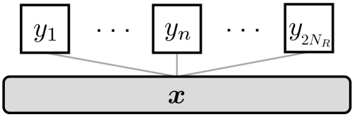
(a) Non-decoupled univariate model in eq. (5b) as the SotA [6, 9, 7, 8].

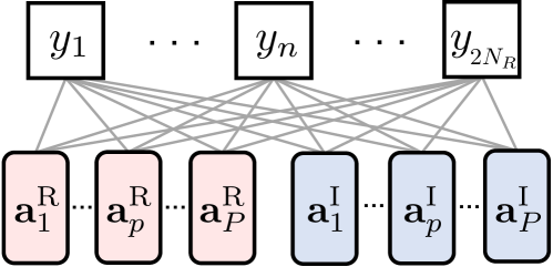
(b) Proposed fully-decoupled $2P$-multivariate UVD model in eq. (9).

Figure 1: Different FG representations of the GQSM system.

In light of the above, the random vector variable $\mathsf{a}$ is introduced to model the unit vectors, where the discrete uniform prior probability mass function (PMF) is given by

$$\mathbb{P}_{\mathsf{a}}(\mathbf{a})\triangleq\frac{1}{N_{T}}\cdot\!\sum_{\mathbf{e}_{t}\in\mathcal{A}}\!\delta(\mathbf{e}_{t}-\mathbf{a}),\vspace{-1.25ex}$$ (8)

where $\mathbf{a}$ denotes an instance of $\mathsf{a}$, $\mathcal{A}\triangleq\{\mathbf{e}_{t}\}_{t=1}^{N_{T}}\in[0,1]^{N_{T}\times 1}$ is the event set of $\mathsf{a}$, and $\delta(\cdot)$ denotes the unit impulse function where $\delta(\bm{x})=1$ if $|\bm{x}|_{0}=0$, and $\delta(\bm{x})=0$ otherwise.

Since the $2P$ vector variables are instances of the variable $\mathsf{a}$, the estimation problem is rewritten into the UVD form as

$$\bm{y}=\bm{H}\begin{bmatrix}\sum_{p=1}^{P}s^{\mathrm{R}}_{p}\mathbf{a}^{\mathrm{R}}_{p}\\ \!\sum_{p=1}^{P}s^{\mathrm{I}}_{p}\mathbf{a}^{\mathrm{I}}_{p}\\ \end{bmatrix}+\bm{w}\in\mathbb{R}^{2N_{R}\times 1},\vspace{-0.5ex}$$ (9)

where the random variables $\mathbf{a}^{\mathrm{R}}_{1},\cdots,\mathbf{a}^{\mathrm{R}}_{P}$ respectively model the unit vectors $\mathbf{e}_{k^{\mathrm{R}}_{1}},\cdots,\mathbf{e}_{k^{\mathrm{R}}_{P}}$ and likewise for $\mathbf{a}^{\mathrm{I}}_{1},\cdots,\mathbf{a}^{\mathrm{I}}_{P}$, which has been illustrated as a factor graph (FG)in Fig. 1(b).

III-B Vector-valued Gaussian Belief Propagation (GaBP)

In light of the above, this section provides the derivation of the purpose-fit vector-valued MP rules operating on the factor graph of Fig. 1(b), based on the Gaussian belief propagation (GaBP) framework [11, 10], assuming perfect channel state information (CSI) at the receiver. This enables the joint estimation of the $2P$ activation vector variables (unit vectors) only within their respective signal domains of size $N_{T}$ each.

First, the soft-replica vectors for the activation vector variables $\mathbf{a}^{\mathrm{R}}_{p}$ and $\mathbf{a}^{\mathrm{I}}_{p}$ for $p\in\{1,\cdots,P\}$ are defined as $\hat{\mathbf{a}}^{\mathrm{R}}_{p:n}$ and $\hat{\mathbf{a}}^{\mathrm{I}}_{p:n}$ respectively for the $n$-th factor node with $n\in\{1,\cdots,2N_{R}\}$. The corresponding expected error covariance matrix of the soft-replica $\hat{\mathbf{a}}^{\mathrm{R}}_{p:n}$ is defined as

$$\mathbf{\Gamma}^{\mathrm{R}}_{p:n}\!\triangleq\mathbb{E}_{\mathsf{a}}[(\mathbf{a}-\hat{\mathbf{a}}^{\mathrm{R}}_{p:n})(\mathbf{a}-\hat{\mathbf{a}}^{\mathrm{R}}_{p:n})^{\!\mathsf{T}}].$$ (10)

Remark: Due to page limitations, the derivations are provided only for the real components (i.e., for $\mathbf{a}^{\mathrm{R}}_{p}$), as the expressions for the respective imaginary components are identical, except for the change of superscripts $(\cdot)^{\mathrm{R}}$ to $(\cdot)^{\mathrm{I}}$ and vice-versa.

In hand of the soft-replicas, the factor nodes perform soft-interference cancellation (IC) on the received signals $y_{n}$ as

$$\bar{y}^{\mathrm{R}}_{p:n}=y_{n}\!-\!{\mathbf{h}_{n}^{\mathrm{R}}}^{\!\mathsf{T}}\!\textstyle\sum_{p^{\prime}\neq p}^{P}(s_{p^{\prime}}^{\mathrm{R}}\hat{\mathbf{a}}_{p^{\prime}:n}^{\mathrm{R}})-{\mathbf{h}_{n}^{\mathrm{I}}}^{\!\!\mathsf{T}}\!\textstyle\sum_{p^{\prime}=1}^{P}(s_{p^{\prime}}^{\mathrm{I}}\hat{\mathbf{a}}_{p^{\prime}:n}^{\mathrm{I}})\vspace{-2.2ex}$$ (11)

$$=\!\underbrace{{\mathbf{h}_{n}^{\mathrm{R}}}^{\!\mathsf{T}}\!\!s_{p}^{\mathrm{R}}\mathbf{a}_{p}^{\mathrm{R}}}_{\text{true symbol}}\!+{\mathbf{h}_{n}^{\mathrm{R}}}^{\!\mathsf{T}}\!\!\!\textstyle\sum\limits_{p^{\prime}\neq p}^{P}\!\!\!s_{p^{\prime}}^{\mathrm{R}}\!(\;\!\!\hat{\mathbf{a}}_{p^{\prime}}^{\mathrm{R}}\!\!-\!\hat{\mathbf{a}}_{p^{\prime}\!:n}^{\mathrm{R}}\!\;\!)\!+\!{\mathbf{h}_{n}^{\mathrm{I}}}^{\!\!\mathsf{T}}\!\!\!\textstyle\sum\limits_{p^{\prime}=1}^{P}\!\!\!s_{p^{\prime}}^{\mathrm{I}}\!(\;\!\!\hat{\mathbf{a}}_{p^{\prime}}^{\mathrm{I}}\!\!-\!\hat{\mathbf{a}}_{p^{\prime}\!:n}^{\mathrm{I}}\!\!\;)\!+\!w_{n},\vspace{-15ex}$$

where ${\mathbf{h}_{n}^{\mathrm{R}}}^{\!\mathsf{T}}\!\!\in\!\mathbb{R}^{1\times N_{T}}$ and ${\mathbf{h}_{n}^{\mathrm{I}}}^{\!\!\mathsf{T}}\!\!\in\!\mathbb{R}^{1\times N_{T}}$ respectively denote the $n$-th rows of the channel components $\bm{H}^{\mathrm{R}}\in\mathbb{R}^{2N_{T}\times N_{T}}$ and $\bm{H}^{\mathrm{I}}\in\mathbb{R}^{2N_{T}\times N_{T}}$ which are defined from $\bm{H}\triangleq[\bm{H}^{\mathrm{R}},\bm{H}^{\mathrm{I}}]$.

The sum of the latter error terms and AWGN term $w_{n}$, excluding the true symbol part, is approximated as a Gaussian scalar via the central limit theorem (CLT), which yield the conditional probability density functions (PDFs) of the soft-IC symbols with respect to a given activation vector $\mathbf{a}^{\mathrm{R}}_{p}$ as

$$\mathbb{P}(\bar{y}_{p:n}^{\mathrm{R}}|\mathbf{a}_{p}^{\mathrm{R}})\propto\exp\!\bigg{(}\!-\!\frac{|\bar{y}_{p:n}^{\mathrm{R}}-s_{p}^{\mathrm{R}}{\mathbf{h}_{n}^{\mathrm{R}}}^{\!\mathsf{T}}\!\mathbf{a}_{p}^{\mathrm{R}}|^{2}}{\nu^{\mathrm{R}}_{p:n}}\bigg{)},\vspace{-1ex}$$ (12)

where the conditional variance $\nu^{\mathrm{R}}_{p:n}$ is obtained by

$$\nu^{\mathrm{R}}_{p:n} =\mathbb{E}\!\left[|\bar{y}_{p:n}^{\mathrm{R}}-s_{p}^{\mathrm{R}}{\mathbf{h}_{n}^{\mathrm{R}}}^{\!\mathsf{T}}\!\mathbf{a}_{p}^{\mathrm{R}}|^{2}\right]$$

$$=\nu_{n}-{\mathbf{h}_{n}^{\mathrm{R}}}^{\!\mathsf{T}}\!\big{(}|s_{p}^{\mathrm{R}}|^{2}\cdot\mathbf{\Gamma}_{p:n}^{\mathrm{R}}\big{)}(\mathbf{h}_{n}^{\mathrm{R}})^{*}+\tfrac{N_{0}}{2},$$ (13)

with $\nu_{n}\!\triangleq\!{\mathbf{h}_{n}^{\mathrm{R}}}^{\!\mathsf{T}}\!\big{(}\!\sum\limits_{p=1}^{P}\!\!|s_{p}^{\mathrm{R}}|^{2}\!\cdot\!\mathbf{\Gamma}_{p:n}^{\mathrm{R}}\big{)}{\mathbf{h}_{n}^{\mathrm{R}}}^{\!*}\!\!+\!{\mathbf{h}_{n}^{\mathrm{I}}}^{\!\!\mathsf{T}}\!\big{(}\!\sum\limits_{p=1}^{P}\!\!|s_{p}^{\mathrm{I}}|^{2}\!\cdot\!\mathbf{\Gamma}_{p:n}^{\mathrm{I}}\big{)}{\mathbf{h}_{n}^{\mathrm{I}}\!}^{*}\!.$

Then, each variable node aggregates the conditional PDFs from the connected factor nodes to compute the extrinsic belief $b_{p:n}^{\mathrm{R}}$ with self-interference cancellation, following

$$\mathbb{P}(b_{p:n}^{\mathrm{R}}|\mathbf{a}_{p}^{\mathrm{R}})=\!\!\prod_{n^{\prime}\neq n}^{2N_{R}}\!\!\mathbb{P}(\bar{y}_{p:n^{\prime}}^{\mathrm{R}}|\mathbf{a}_{p}^{\mathrm{R}})\propto e^{({\bm{\eta}^{\mathrm{R}}_{p:n}\!\!\!\!}^{\mathsf{T}}\mathbf{a}_{p}^{\mathrm{R}}-\tfrac{1}{2}{\mathbf{a}_{p}^{\mathrm{R}}}^{\mathsf{T}}\mathbf{\Lambda}^{\mathrm{R}}_{p:n}\mathbf{a}_{p}^{\mathrm{R}})},\vspace{-1ex}$$ (14)

where $\bm{\eta}_{p:n}^{\mathrm{R}}$ and $\mathbf{\Lambda}_{p:n}^{\mathrm{R}}$ are the information vector and the precision matrix of the extrinsic belief $b_{p:n}^{\mathrm{R}}$, given by

$$\bm{\eta}_{p:n}^{\mathrm{R}}\!=\!s^{\mathrm{R}}_{p}\!\sum_{n^{\prime}\neq n}^{2N_{R}}\!\frac{\bar{y}^{\mathrm{R}}_{p:n^{\prime}}}{\nu^{\mathrm{R}}_{p:n^{\prime}}}\mathbf{h}_{n^{\prime}}^{\mathrm{R}}\;\text{and}\;\mathbf{\Lambda}_{p:n}^{\mathrm{R}}\!=\!|s_{p}^{\mathrm{R}}|^{2}\!\!\sum_{n^{\prime}\neq n}^{2N_{R}}\!\frac{\mathbf{h}_{n^{\prime}}^{\mathrm{R}}{\mathbf{h}_{n^{\prime}}^{\mathrm{R}}}^{\!\!\mathsf{T}}\!}{\nu^{\mathrm{R}}_{p:{n^{\prime}}}}.\vspace{-1ex}$$ (15)

In turn, the posterior Bayes-optimal soft-replicas are computed from the extrinsic beliefs via

$$\hat{\mathbf{a}}_{p:n}^{\mathrm{R}}\!=\!\dfrac{\mathbb{E}_{\mathsf{a}}[\mathbf{a}\cdot\mathbb{P}(b_{p:n}^{\mathrm{R}}|\mathbf{a})]}{\mathbb{E}_{\mathsf{a}}[\mathbb{P}(b_{p:n}^{\mathrm{R}}|\mathbf{a})]}\!=\!\dfrac{\sum_{q=1}^{N_{T}}\mathbf{a}_{q}\cdot\mathbb{P}(b_{p:n}^{\mathrm{R}}|\mathbf{a}_{q})\cdot\mathbb{P}(\mathbf{a}_{q})}{\sum_{q^{\prime}=1}^{N_{T}}\mathbb{P}(b_{p:n}^{\mathrm{R}}|\mathbf{a}_{q^{\prime}})\cdot\mathbb{P}(\mathbf{a}_{q^{\prime}})},\!\!\!\!\vspace{-0.5ex}$$ (16)

while the corresponding error covariance matrix is given by

$$\mathbf{\Gamma}_{p:n}^{\mathrm{R}} \triangleq\mathbb{E}_{{\mathsf{a}}}[(\mathbf{a}-{\hat{\mathbf{a}}}_{p:n}^{\mathrm{R}})(\mathbf{a}_{p}-\hat{{\mathbf{a}}}_{p:n}^{\mathrm{R}})^{\mathsf{H}}].$$ (17)

Equations (11)-(17) describe the steps of one MP iteration to estimate the $2P$ activation vectors of the GQSM reformulated as eq. (9), which yields the refined posterior soft-replica vectors and the corresponding error covariance matrices. In addition, at the end of such $\tau$-th MP iteration, the soft-replica vectors and the error covariance matrices are updated with damping [12] to prevent an early convergence to a local optima [13, 14], following $x^{[\tau+1]}\!\leftarrow\!\rho x^{[\tau]}\!+\!(1-\rho)x^{[\tau+1]}$ where $\rho\in[0,1]$ is the damping factor, and $\tau$ is the iteration number.

Next, to obtain the hard-decisions on the $2P$ activation vectors, a the information is aggregated between all $2N_{R}$ factor nodes to compute the consensus beliefs (i.e., eq. (14) without the self-interference cancellation), which yields the extrinsic consensus PDFs of the belief $b_{p}^{\mathrm{R}}$.

Finally, the optimal activation vector estimate is selected by evaluating the PDFs for the $N_{T}$ valid states of $\mathbf{a}\in\mathcal{A}$ i.e.,

$$\tilde{\mathbf{a}}^{\mathrm{R}}_{p}=\underset{\mathbf{a}\in\mathcal{A}}{\mathrm{argmax}}~{}\mathbb{P}(b_{p}^{\mathrm{R}}|\mathbf{a}).\vspace{-1ex}$$ (18)

The proposed UVD-GaBP decoder for pilotted GQSM, described by eq. (10)-(18), is summarized in Algorithm 1.

1: Inputs: Received signal $\bm{y}$, effective channels $\bm{H}^{\mathrm{R}}$ and $\bm{H}^{\mathrm{I}}$,

2:       pilot symbols $s^{\mathrm{R}}_{p},s^{\mathrm{I}}_{p}\;\forall p$, and noise variance $N_{0}$.

3: Outputs: Estimated activation vectors $\tilde{\mathbf{a}}^{\mathrm{R}}_{p}$ and $\tilde{\mathbf{a}}^{\mathrm{I}}_{p}\;\forall p$.

4:

5: Initialization: $\forall n$ and $\forall p$,

6:Initialize $\hat{\mathbf{a}}^{\mathrm{R}}_{p:n},\hat{\mathbf{a}}^{\mathrm{I}}_{p:n}$;

7:Compute $\mathbf{\Gamma}^{\mathrm{R}}_{p:n},\mathbf{\Gamma}^{\mathrm{I}}_{p:n}$ via eq. (10);

8: MP iterations for $\tau=1,\cdots,\tau_{\mathrm{max}}$, $\;\forall n$ and $\forall p$,

9:For both real and imaginary components:

10:Perform soft-IC via eq. (11);

11:Compute $\nu^{\mathrm{R}}_{p:n},\nu^{\mathrm{I}}_{p:n}$ via eq. (III-B);

12:Compute $\bm{\eta}_{p:n}^{\mathrm{R}},\bm{\eta}_{p:n}^{\mathrm{I}}$ and $\mathbf{\Lambda}_{p:n}^{\mathrm{R}},\mathbf{\Lambda}_{p:n}^{\mathrm{I}}$ via eq. (15);

13:Compute $\hat{\mathbf{a}}_{p:n}^{\mathrm{R}},\hat{\mathbf{a}}_{p:n}^{\mathrm{I}}$ via eq. (16);

14:Compute $\mathbf{\Gamma}_{p:n}^{\mathrm{R}},\mathbf{\Gamma}_{p:n}^{\mathrm{I}}$ via eq. (17);

15:Update $\hat{\mathbf{a}}^{\mathrm{R}}_{p:n},\hat{\mathbf{a}}^{\mathrm{I}}_{p:n}$ via a damped update [12, 13];

16: end for

17:Obtain $\tilde{\mathbf{a}}^{\mathrm{R}}_{p}$, $\tilde{\mathbf{a}}^{\mathrm{I}}_{p}$ via eq. (18);

Algorithm 1 ​​: Proposed UVD-GaBP GQSM Decoder

IV Performance Evaluation

IV-A Simulation Results

In Fig. 2, GQSM simulation results are provided for mMIMO systems with $N_{T}=16$ and $32$, and varying values of $P$, where the performance is evaluated in terms of the BER against the $E_{b}/N_{0}$ (signal-to-noise ratio (SNR) per bit).

Note the extremely low $E_{b}/N_{0}$ ranges of the GQSM, which benefits from the fact that most information is encoded without using any transmission power, corroborating the original motivation of enabling energy- and spectral-efficient mMIMO.

Since the computational complexity of the brute-force ML and SotA decoders are prohibitive in the considered system scales, a Genie-aided matched filter bound (MFB)[15] is introduced instead as an absolute performance bound, which is obtained by providing the UVD-GaBP method with perfect prior knowledge of the activation vectors and pilot symbols.

Fig. 2 demonstrates the efficient demodulation capability of the proposed UVD-GaBP decoder for high-rate GQSM signals in $16\times 16$ and $32\times 32$ mMIMO setups, even with the affordable computational power of an average personal computer. It can be observed that optimal performance is achieved by the UVD-GaBP for $P=1$ in both scenarios, and a slight performance loss of about $1\!\sim\!2\mathrm{dB}$ and an error-floor is exhibited at high $E_{b}/N_{0}$, for increasing $P\geq 1$. However, notice that the negative effect in both the BER performance and the error-floor is reduced in the larger system with $N_{T}=32$, which benefits from the increased sparsity in the system and the consequently increased orthogonality in the unit vector random variables.

Further improvements including the elimination of error-floors can be expected if the joint distributions of the activation vectors and their non-uniform prior distributions are introduced in the MP design, and a non-piloted variation of the method is also under investigation, which will be addressed in an upcoming journal article.

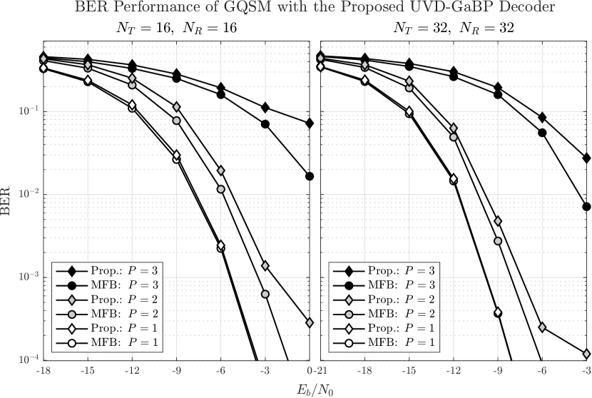
Figure 2: BER performance of the proposed (Prop.) UVD-GaBP decoder and its Genie-aided MFB.

IV-B Complexity Analysis

Table I compares the decoding complexity of the proposed UVD-GaBP method against few SotA algorithms, where it can be seen that the SotA methods have reduced the squared-combinatorial term appearing in the brute-force ML search.

Namely, the relaxed orthogonal matching pursuit-based ordered successive IC (ROMP-OSIC) decoder proposed in [9] relaxes the upper index of the binomial coefficient by a factor $N_{v}$ with $P\!\leq\!N_{v}\!\leq\!N_{T}$, whereas the IQ-decoupled GaBP decoder proposed in [10] eliminates the quadratic factor on the binomial coefficient, and $\tau_{\mathrm{max}}$ is the number of MP iterations. However, the SotA methods still retain the binomial coefficient which is not scalable to mMIMO system of consideration.

On the other hand, the proposed UVD-GaBP decoder enjoys a significantly reduced complexity which is completely independent of the binomial coefficient, enabling the decodability of GQSM schemes in significantly larger mMIMO systems, as verified in the performance evaluation results.

TABLE I: Complexity orders of various GQSM decoders.

GQSM Decoding Algorithm	Decoding Complexity Order
Brute-force ML Search [4]	$\mathcal{O}\big{[}\binom{N_{T}}{P}{}^{\!2}PN_{R}\big{]}$
ROMP-OSIC [9]	$\mathcal{O}\big{[}\binom{N_{v}}{P}{}^{\!2}{N_{v}}^{2}PN_{T}N_{R}\big{]}$
IQ-decoupled GaBP [10]	$\mathcal{O}\big{[}\;\!\tau_{\mathrm{max}}\!\cdot\!\binom{N_{T}}{P}{N_{T}}^{2}N_{R}\big{]}$
Proposed UVD-GaBP	$\mathcal{O}\big{[}\;\!\tau_{\mathrm{max}}\!\cdot\!P{N_{T}}^{2}N_{R}\big{]}$

V Conclusion

We paved the way towards feasible energy- and spectral-efficient mMIMO systems with high-performance GQSM, by proposing a novel GaBP-based decoder exploiting a UVD of the GQSM signal model and pilots, which is shown to achieve a complexity order that is independent of combinatorial factors. Simulation results verify the effectiveness of the method.

In addition, the multi-user scenario should also be considered to support the B5G mMIMO access expectations.

References

- [1] R. Y. Mesleh, H. Haas, S. Sinanovic, C. W. Ahn, and S. Yun, “Spatial modulation,” IEEE Trans. Veh. Technol., vol. 57, no. 4, pp. 2228–2241, Jul. 2008.
- [2] Z. Zhang, Y. Xiao, Z. Ma, M. Xiao, Z. Ding, X. Lei, G. K. Karagiannidis, and P. Fan, “6G wireless networks: Vision, requirements, architecture, and key technologies,” IEEE Veh. Technol. Mag., vol. 14, no. 3, pp. 28–41, 2019.
- [3] T. S. Rappaport, Y. Xing, O. Kanhere, S. Ju, A. Madanayake, S. Mandal, A. Alkhateeb, and G. C. Trichopoulos, “Wireless communications and applications above 100 GHz: Opportunities and challenges for 6G and beyond,” IEEE Access, vol. 7, pp. 78 729–78 757, 2019.
- [4] R. Mesleh, S. S. Ikki, and H. M. Aggoune, “Quadrature spatial modulation,” IEEE Trans. Veh. Technol., vol. 64, no. 6, pp. 2738–2742, Jun. 2015.
- [5] E. Başar, U. Aygölü, E. Panayirci, and H. V. Poor, “Space-time block coded spatial modulation,” IEEE Transactions on Communications, vol. 59, no. 3, pp. 823–832, 2011.
- [6] H. S. Rou, G. T. F. Abreu, H. Iimori, D. González G., O. Gonsa, “Scalable quadrature spatial modulation,” 2022, submitted to Trans. Wireless Commun.
- [7] L. Wang and Z. Chen, “Enhanced diversity-achieving quadrature spatial modulation with fast decodability,” IEEE Trans. Veh. Technol., vol. 69, no. 6, pp. 6165–6177, 2020.
- [8] J. Li, X. Jiang, Y. Yan, W. Yu, S. Song and M. Lee, “Low complexity detection for quadrature spatial modulation systems,” Wireless Person. Commun., vol. 95, no. 4, pp. 4171–4183, 2017.
- [9] J. An, C. Xu, Y. Liu, L. Gan, and L. Hanzo, “The achievable rate analysis of generalized quadrature spatial modulation and a pair of low-complexity detectors,” IEEE Transactions on Vehicular Technology, vol. 71, no. 5, pp. 5203–5215, 2022.
- [10] H. S. Rou, G. T. F. de Abreu, and T. Takahashi, “An efficient vector-valued belief propagation decoder for quadrature spatial modulation,” in 2022 56th Asilomar Conference on Signals, Systems, and Computers, 2022, pp. 27–31.
- [11] D. Bickson, “Gaussian belief propagation: Theory and aplication,” arXiv preprint arXiv:0811.2518, 2008.
- [12] P. Som, T. Datta, A. Chockalingam and B. S. Rajan, “Improved large-mimo detection based on damped belief propagation,” in IEEE Inf. Theory Workshop on Inf. Theory, 2010, pp. 1–5.
- [13] Q. Su and Y.-C. Wu, “On convergence conditions of gaussian belief propagation,” IEEE Transactions on Signal Processing, vol. 63, no. 5, pp. 1144–1155, 2015.
- [14] J. Du, S. Ma, Y.-C. Wu, S. Kar, and J. M. Moura, “Convergence analysis of distributed inference with vector-valued gaussian belief propagation.” J. Mach. Learn. Res., vol. 18, no. 1, pp. 6302–6339, 2017.
- [15] T. Takahashi, S. Ibi, and S. Sampei, “Design of adaptively scaled belief in multi-dimensional signal detection for higher-order modulation,” IEEE Trans. Commun., vol. 67, no. 3, pp. 1986–2001, 2019 2019.