Provable Tensor Completion with Graph Information

Abstract

Graphs, depicting the interrelations between variables, has been widely used as effective side information for accurate data recovery in various matrix/tensor recovery related applications. In this paper, we study the tensor completion problem with graph information. Current research on graph-regularized tensor completion tends to be task-specific, lacking generality and systematic approaches. Furthermore, a recovery theory to ensure performance remains absent. Moreover, these approaches overlook the dynamic aspects of graphs, treating them as static akin to matrices, even though graphs could exhibit dynamism in tensor-related scenarios. To confront these challenges, we introduce a pioneering framework in this paper that systematically formulates a novel model, theory, and algorithm for solving the dynamic graph regularized tensor completion problem. For the model, we establish a rigorous mathematical representation of the dynamic graph, based on which we derive a new tensor-oriented graph smoothness regularization. By integrating this regularization into a tensor decomposition model based on transformed t-SVD, we develop a comprehensive model simultaneously capturing the low-rank and similarity structure of the tensor. In terms of theory, we showcase the alignment between the proposed graph smoothness regularization and a weighted tensor nuclear norm. Subsequently, we establish assurances of statistical consistency for our model, effectively bridging a gap in the theoretical examination of the problem involving tensor recovery with graph information. In terms of the algorithm, we develop a solution of high effectiveness, accompanied by a guaranteed convergence, to address the resulting model. To showcase the prowess of our proposed model in contrast to established ones, we provide in-depth numerical experiments encompassing synthetic data as well as real-world datasets.

1 Introduction

Graphs have emerged as a crucial tool for modeling a plethora of structured or relational systems, such as social networks, knowledge graphs, and academic graphs, and been widely used in many applications including intelligent transportation system [1, 2], moving object segmentation [3, 4], object tracking [5, 6], recommendation system [7, 8] and bioinformatics [9, 10], to name a few. Specifically, in many matrix/tensor completion related tasks, graphs can serve as side information illustrating the connections among variables (e.g., the social networks of users in collaborative filtering tasks, one of the most common applications of matrix/tensor completion), where nodes represent the entities while edges capture the pairwise similarities between these entities. The similarity graphs construct potential geometric structures in the data, and thus can be exploited as effective priors for better recovery. Basically, the problem of matrix/tensor completion with graph information is to recover the original matrix/tensor from its partial observations, where some supplementary similarity graphs are accessible. With the increasing popularity of graph-structured data, matrix/tensor completion with graph information has caught increasing attentions in recent years, and delivered successful applications in various domains such as recommendation system [11, 12], network latency estimation [13], bioinformatics [14, 15, 16, 17], social image retagging [18] and intelligent transportation system [19, 20].

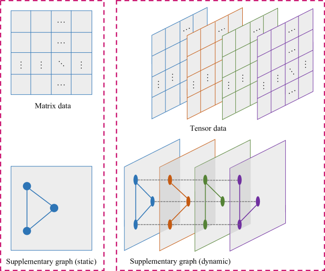
Figure 1: The illustration of matrix with static graph (left) and tensor with dynamic graph (right), where different layers represent different states (e.g., time periods), dots represent vertices of the graph, solid lines denote the edges, and dots connected by gray dashed lines means that they are the same vertex in different states.

As the multidimentional generalization of vector and matrix, tensor provides a natural presentation form for a wide variety of real-world data to deliver the inherent structure information, and has thus become an important tool in many areas. However, compared with matrices, the higher dimensions of tensors makes them more prone to missing data, and the sparser observations also increase the difficulty of data recovery. Hence, tensor completion (TC) poses a more intricate challenge than matrix completion (MC), demanding a greater reliance on structural prior information. In numerous real-world applications, the underlying tensors often exhibit low-rank structures. This characteristic has sparked extensive research endeavors aiming to leverage this low-rank nature within TC [21, 22]. Throughout recent decades, an array of tensor rank definitions has emerged, encompassing CANDECOMP/PARAFAC (CP) rank [23], Tucker rank [24, 25], tensor train (TT) rank [26], tensor ring (TR) rank [27]. Each of these definitions offers distinct advantages and limitations. Recently, tensor singular value decomposition (t-SVD) [28, 29] and the induced tensor tubal rank [30] has drawn considerable interest due to its advantages in the exploitation of the global structure information and spatial-shifting correlations ubiquitous in real-world tensor data [31, 22], and thus has been explored in many recent researches for tensor recovery [32, 33, 34, 35].

In many TC related real-world applications, relying solely on low-rankness often fails to achieve satisfactory recovery performance, particularly when only a few observations are available, which urges the exploration of exploiting the geometric structures underlying in the similarity graphs in low-rank TC tasks. Over the recent years, there have been several studies addressing MC with graph information [36, 37, 38, 39]. These studies showcase how incorporating additional graphs can enhance recovery performance. Nonetheless, the shift from MC to higher-order TC presents significant challenges, mainly arising from the dynamic nature of graphs within tensor data. In the case of matrices, graphs are oftentimes static, meaning they remain constant and unchanging after construction. In contrast, in higher-order tensor scenarios, the relationships between variables can evolve and alter with changing circumstances or varying states. For instance, in the movie recommender system, the social network of users may vary over time, with new connections forming between previously unconnected individuals (some strangers establish social contact) and existing relationships fading away (some acquaintances lose touch). Fig. 1 illustrates a matrix with static graph and a tensor with dynamic graph.

The dynamic nature of graphs presents a twofold challenge, both in terms of mathematical modeling and theoretical analysis, when addressing the problem of TC with graph information. As a consequence, existing research predominantly adheres to a matrix-based approach, where graphs are assumed to be static. This approach directly applies the graph smoothness modeling strategy from matrix case, employing graph Laplacian regularization based on Laplacian matrices. However, this implementation disrupts the inherent structure of tensors and their corresponding graphs, leading to a decline in recovery performance. Moreover, current studies on graph-regularized TC tend to be task-specific. For example, studies such as [13] focuses on network latency estimation, while [16] and [17] deal with microRNA-disease association prediction, [18] tackles social image retagging, and [19] addresses traffic data imputation. Yet, these approaches lack a comprehensive and generalized methodology, resulting in a lack of systematic coverage. Furthermore, the absence of a recovery theory for TC with graph information undermines the assurance of recovery performance, casting doubt on their reliability for real-world applications. In the absence of proper guarantees or statistical consistency analysis, the effectiveness and applicability of these methods become uncertain. Hence, an immediate necessity arises to formulate a unified framework for TC incorporating dynamic graph information. This framework should encompass a mathematical model, theoretical assurances, and an efficient algorithm, all geared towards fulfilling the requirements of practical applications.

To address the aforementioned concerns, there are four main issues to be considered: (1) how to rigorously represent the dynamic graph mathematically; (2) how to holistically characterize the pairwise similarity structure of the tensor underlying in the dynamic graph; (3) how to build the overall model and efficient algorithm to exploit the low-rank and pairwise similarity structure of the tensor simultaneously for tensor recovery; (4) how to establish theoretical guarantees of the resulting model to ensure the recovery performance. In view of this, taking full account of the dynamic nature of the graphs, we establish in this paper a rigorous mathematical representation and propose a new tensor-oriented graph smoothness regularization for dynamic graphs, based on which we develop a novel model for TC with dynamic graph information. The new regularization exploits the tensor’s global pairwise similarity structure underlying in the dynamic graph as a whole, and it can be seen that it incorporates the static graph in matrix scenarios as a special case. Theoretically, we demonstrate that the proposed graph smoothness regularization is equivalent to a weighted tensor nuclear norm, where the weights implicitly characterize the graph information, based on which we establish statistical consistency guarantees for our model. As far as we know, this is the first theoretical recovery outcome for the graph-regularized tensor recovery model, effectively filling a gap in the theoretical analysis of tensor recovery involving graph information.

In summary, the main contributions of this paper are as follows:

• Taking the dynamic nature of the graphs into consideration, we establish a rigorous mathematical representation of the dynamic graph. With this foundation, we formulate a novel tensor-oriented graph smoothness regularization technique, leveraging the inherent pairwise similarity structure intrinsic to the overall dynamic graph.

• We develop a new model for TC with dynamic graph information, which combines transformed t-SVD and the above graph smoothness regularization to exploit the low-rank and pairwise similarity structure of the tensor simultaneously. Furthermore, we develop an effective algorithm with convergence guarantee based on alternating direction method of multiplier (ADMM).

• Employing a tensor atomic norm as a bridge, we establish the equivalence between the proposed graph smoothness regularization and a weighted tensor nuclear norm, and then derive statistical consistency guarantees for our model. As far as we are aware, this represents the first established theoretical guarantee within the field of research focused on graph regularized tensor recovery.

• Thorough experiments are undertaken using both synthetic and real-world datasets, showcasing the efficacy of the introduced graph smoothness regularization approach. The outcomes emphasize the superiority of our method compared to state-of-the-art TC techniques, particularly when dealing with scenarios featuring limited available observations.

The remainder of this paper is organized as follows. In Section 2 we provide a brief survey on the low-rank TC and MC/TC with graph information. The main notations and preliminaries are introduced in Section 3. We present our main model in Section 4 and the optimization algorithm in Section 5. Consistency guarantees of the proposed model is established in Section 6, and numerical experiments on synthetic and real data are conducted in Section 7. Finally, in Section 8 we conclude this paper and provide potential extensions of our method.

2 Related work

2.1 Low-rank Tensor Completion

Generally speaking, the existing representative methods for low-rank TC can be classified based on the employed tensor decomposition schemes and corresponding definitions of tensor rank, and the commonest two decomposition strategies are CP [23] and Tucker [24] decomposition. For CP decomposition based TC, Ashraphijuo et al. [40] proposed a low CP rank approach for TC and derived fundamental conditions on the sampling pattern for tensor completability given its CP rank. Ghadermarzy et al. [41] proposed an atomic M-norm as a convex proxy of tensor CP rank resulting in nearly optimal sample complexity for low-rank TC. Zhao et al.  [42] formulate CP factorization using a fully Bayesian treatment to achieve automatic CP rank determination. For Tucker decomposition based TC, Liu et al. [43] first developed the sum of nuclear norms (SNN) of all unfolding matrices of a tensor to approximate its Tucker rank. Then, Romera-Paredes and Pontil [44] proved that the SNN is not the tightest convex relaxation of the Tucker rank. Mu et al. [45] shown that SNN can be substantially suboptimal, and introduce a new convex relaxation of Tucker rank based on a more balanced tensor unfolding matrix. Some other TC approaches based on Tucker decomposition can be referred to [46, 47].

In the past few years, the t-SVD decomposition has also been studied in low-rank TC problem. Semerci et al. [48] first proposed a tensor nuclear norm (TNN) regularization to approximate the sum of its multi-rank, then Zhang et al. [49] shown that TNN was a convex envelope. Moreover, Zhang and Aeron [50] investigated the low-tubal-rank TC problem through TNN and established a theoretical bound for exact recovery. Based on tensor tubal rank, Zhou et al. [51] proposed a new tensor factorization method for low-rank TC with a higher algorithm efficiency. Recently, inspired by the t-product based on any invertible linear transforms [29], Lu et al. [52] generalized the definitions of tensor tubal rank and TNN, based on which a convex TNN minimization model was proposed for TC, and meanwhile a optimal bound for the guarantee of exact recovery was given. Very recently, Zhang et al. [21] studied the third-order TC problem with Poisson observations based on t-SVD. Some more t-SVD based TC approaches can be referred to [53, 54]. In addition to the above-mentioned ones, some other tensor decomposition strategies are also introduced into TC problem, such as tensor train (TT) [55] and tensor ring (TR) [56]. Due to that they usually need to reshape the original tensor into a higher-order one, TT/TR-based approaches unavoidably suffer from the high computational cost.

2.2 Matrix/tensor Completion with Graph Information

In the past decade, there have been some studies on the MC and TC with graph information. For the matrix case, Zhou et al. [57] introduced Gaussian process prior in MC to capture the underlying covariance structures, which enabled the efficient incorporation of graph information. Kalofolias et al. [36] introduced graph Laplacian as regularization terms in the nuclear norm minimization based model to constrain the solution to be smooth on graphs. Following that, Rao et al. [37] further derived consistency guarantees for graph regularized MC. Elmahdy et al. [38] developed a hierarchical stochastic block model to refine the matrix ratings by hierarchical graph clustering. Very recently, Dong et al. [39] proposed a efficient Riemannian gradient descent based algorithm to solve the model in [37], while there was no further theoretical contribution. In addition, graph information has also been employed in many MC based specific tasks such as recommendation system [11, 12], microRNA-disease association prediction [14, 15] and traffic status prediction [58].

As for the tensor case, the existing studies are basically oriented toward specific tasks, i.e., construct different static graphs for different tasks and then employ the similar approach as in matrix scenarios. Hu et al. [13] used the geometrical structure information of the nodes to construct a graph Laplacian regularization constraint in tensor nuclear norm minimization model to estimate network latency. Tang et al. [18] construct an anchor-unit graph and define the similarity regularization in tensor Tucker decomposition model to refine the tags of social images. Deng et al. [19] and Nie et al. [20] employ traffic networks as spatial regularization in TC for traffic data imputation and speed estimation, respectively. Ouyang et al. [17] and Huang et al.[16] use biological similarity network and features as relational constraints to predict multiple types of microRNA-disease associations, respectively. In addition, Guan et al. [59] proposed a general graph-regularized TC model which employed CP decomposition to leverage the low-rank structure, and meanwhile applied graph Laplacian regularization for static graph exploitation, also following the approach in matrix scenarios.

It is obviously more blunt to directly incorporate the graph smoothness constraints of matrix scenarios, i.e., graph Laplacian regularization for static graph, into the problem of TC with graph information, disrupting the overall structure of the tensor and dynamic nature of the corresponding graphs. Meanwhile, there is not any theoretical guarantees for TC with graph information to ensure the recovery performance. To this aim, our main focus of this study is to establish a coherent model with solid theoretical guarantees for the problem of TC with dynamic graph information.

3 Notations and Preliminaries

3.1 Notations

We first summarize some basic notations used throughout this paper. We use lowercase letters, bold lowercase letters, capital letters and calligraphic letters to denote scalars, vectors, matrices and tensors, respectively, e.g., $x,\mathbf{x},X,\mathcal{X}$. In this work, we focus on the three-order tensors which is the most common case in practical applications, and leave the higher-order case as a future study. For a order-$3$ tensor $\mathcal{X}\in\mathbb{R}^{n_{1}\times n_{2}\times n_{3}}$, its $(i_{1},i_{2},i_{3})$-th entry is denoted by $\mathcal{X}_{i_{1}i_{2}i_{3}}$, its Frobenius norm is defined by $\|\mathcal{X}\|_{F}=\sqrt{\sum_{i_{1},i_{2},i_{3}}\lvert\mathcal{X}_{i_{1}i_{2}i_{3}}\rvert^{2}}$, its infinity norm is defined by $\|\mathcal{X}\|_{\infty}=\max_{i_{1},i_{2},i_{3}}\lvert\mathcal{X}_{i_{1}i_{2}i_{3}}\rvert$, and the inner product between two tensors $\mathcal{X},\mathcal{Y}\in\mathbb{R}^{n_{1}\times n_{2}\times n_{3}}$ is defined by $\left\langle\mathcal{X},\mathcal{Y}\right\rangle=\sum_{i_{1},i_{2},i_{3}}\mathcal{X}_{i_{1}i_{2}i_{3}}\mathcal{Y}_{i_{1}i_{2}i_{3}}$. Specifically, the $i$-th horizontal, lateral, and frontal slice of a third-order tensor $\mathcal{X}$ is denoted by $\mathcal{X}_{i::}$, $\mathcal{X}_{:i:}$ and $\mathcal{X}_{::i}$ (the frontal slice can also be denoted as $\mathcal{X}^{(i)}$ for brevity), and its $(i,j)$-th tube fiber (also called mode-3 fiber) is denoted by $\mathcal{X}_{ij:}$.

3.2 Tensor Singular Value Decomposition

In this subsection, we briefly review the related definitions of transformed t-SVD of three-order tensors.

For a tensor $\mathcal{X}\in\mathbb{R}^{n_{1}\times n_{2}\times n_{3}}$, we define its mode-3 unfolding matrix as $\mathcal{X}_{(3)}\in\mathbb{R}^{n_{3}\times n_{1}n_{2}}$. Then for a matrix $A\in\mathbb{R}^{m\times n_{3}}$, we can define the tensor-matrix product $\mathcal{X}\times_{3}A$ by computing matrix-matrix product $A\mathcal{X}_{(3)}$ and then reshaping the result to an $n_{1}\times n_{2}\times m$ tensor [25]. Let $M\in\mathbb{R}^{n_{3}\times n_{3}}$ be any invertible linear transform matrix such that $MM^{T}=M^{T}M=CI$, where $I$ is the identity matrix and $C$ is a constant. Then for tensor $\mathcal{X}\in\mathbb{R}^{n_{1}\times n_{2}\times n_{3}}$, we use hat notation to denote its mapping tensor in the transform domain specified by $M$: $\widehat{\mathcal{X}}:=\mathcal{X}\times_{3}M$, and $\widetilde{\mathcal{X}}:=\mathcal{X}\times_{3}M^{-1}$ to denote the mapping tensor in the inverse transform domain. Furthermore, for a tensor $\mathcal{X}\in\mathbb{R}^{n_{1}\times n_{2}\times n_{3}}$ and its corresponding $\widehat{\mathcal{X}}$, we define $\overline{\mathcal{X}}$ as a block diagonal matrix composed of each frontal slice of $\widehat{\mathcal{X}}$, i.e.,

$$\overline{\mathcal{X}}=\text{blockdiag}(\widehat{\mathcal{X}})=\begin{pmatrix}\widehat{\mathcal{X}}^{(1)}&&&\\ &\widehat{\mathcal{X}}^{(2)}&&\\ &&\ddots&\\ &&&\widehat{\mathcal{X}}^{(n_{3})}\end{pmatrix},$$

and the inverse permutation of $\text{blockdiag}(\cdot)$ is denoted as $\text{fold}(\cdot)$: $\text{fold}(\text{blockdiag}(\mathcal{X}))=\mathcal{X}$. Then we can define the t-product of two tensors as follows:

Definition 1 (tensor-tensor product (t-product); [29]):

The t-product of tensors $\mathcal{A}\in\mathbb{R}^{n_{1}\times n_{2}\times n_{3}}$ and $\mathcal{B}\in\mathbb{R}^{n_{2}\times n_{4}\times n_{3}}$ under invertible linear transform $M\in\mathbb{R}^{n_{3}\times n_{3}}$, denoted by $\mathcal{A}*_{M}\mathcal{B}$, is a tensor $\mathcal{C}\in\mathbb{R}^{n_{1}\times n_{4}\times n_{3}}$ given by

$$\mathcal{C}=\mathcal{A}*_{M}\mathcal{B}=\text{fold}(\overline{\mathcal{A}}\cdot\overline{\mathcal{B}})\times_{3}M^{-1}.$$ (1)

Furthermore, we use $\star$ to denote the frontal slice-wise matrix-matrix product of two tensors, meaning that $\mathcal{C}=\mathcal{A}\star\mathcal{B}$ is defined by $\mathcal{C}^{(i)}=\mathcal{A}^{(i)}\mathcal{B}^{(i)},i=1,2,...,n_{3}$, for brevity.

Then we introduce the following definitions that will be used later.

Definition 2 (conjugate transpose; [29]):

Given tensor $\mathcal{A}\in\mathbb{R}^{n_{1}\times n_{2}\times n_{3}}$, its conjugate transpose under $*_{M}$, denoted by $\mathcal{A}^{T}$, is a $n_{2}\times n_{1}\times n_{3}$ tensor defined by

$$\text{blockdiag}(\widehat{\mathcal{A}^{T}})=\text{blockdiag}(\widehat{\mathcal{A}})^{T}.$$ (2)

Definition 3 (identity tensor; [29]):

If tensor $\widehat{\mathcal{I}}\in\mathbb{R}^{n_{1}\times n_{2}\times n_{3}}$ satisfies $\widehat{\mathcal{I}}^{(i)}=I$ for $i=1,2,...,n_{3}$, then $\mathcal{I}=\widehat{\mathcal{I}}\times_{3}M^{-1}$ is the identity tensor under $*_{M}$.

Definition 4 (f-diagonal tensor; [29]):

A tensor is f-diagonal if each of its frontal slices is a diagonal matrix.

Definition 5 (unitary tensor; [29]):

A tensor $\mathcal{A}\in\mathbb{R}^{n_{1}\times n_{2}\times n_{3}}$ is unitary under $*_{M}$ if it satisfies $\mathcal{A}^{T}*_{M}\mathcal{A}=\mathcal{A}*_{M}\mathcal{A}^{T}=\mathcal{I}$.

Definition 6 (transformed t-SVD; [29]):

The transformed t-SVD of tensor $\mathcal{A}\in\mathbb{R}^{n_{1}\times n_{2}\times n_{3}}$ under $*_{M}$ is defined as

$$\mathcal{A}=\mathcal{U}*_{M}\mathcal{S}*_{M}\mathcal{V}^{T},$$ (3)

where $\mathcal{U}\in\mathbb{R}^{n_{1}\times n_{1}\times n_{3}}$ and $\mathcal{V}\in\mathbb{R}^{n_{2}\times n_{2}\times n_{3}}$ are unitary tensors, and $\mathcal{S}\in\mathbb{R}^{n_{1}\times n_{2}\times n_{3}}$ is a f-diagonal tensor.

Definition 7 (tensor tubal rank; [52]):

For a tensor $\mathcal{A}\in\mathbb{R}^{n_{1}\times n_{2}\times n_{3}}$ with transformed t-SVD $\mathcal{A}=\mathcal{U}*_{M}\mathcal{S}*_{M}\mathcal{V}^{T}$, its tubal rank is defined as the number of nonzero tube fibers of $\mathcal{S}$.

Definition 8 (tensor spectral norm; [52]):

The spectral norm of a tensor $\mathcal{A}\in\mathbb{R}^{n_{1}\times n_{2}\times n_{3}}$ under $*_{M}$ is $\|\mathcal{A}\|:=\|\overline{\mathcal{A}}\|$.

Definition 9 (tensor nuclear norm; [52]):

The nuclear norm of a tensor $\mathcal{A}\in\mathbb{R}^{n_{1}\times n_{2}\times n_{3}}$ under $*_{M}$ is defined as $\|\mathcal{A}\|_{*}:=\frac{1}{C}\|\overline{\mathcal{A}}\|_{*}$, where $C$ is the constant for $MM^{T}=M^{T}M=CI$.

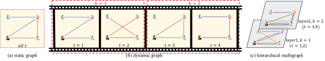
Figure 2: The illustration of (a) static graph, (b) dynamic graph with $T=4$ time periods and (c) corresponding hierarchical multigraph with $K=2$ and width of sliding time window $\frac{T}{K}=2$, using a social network of users as the example.

3.3 Problem Formulation

In this subsection we construct a basic model for low-rank TC based on transformed t-SVD. The reason why we employ transformed t-SVD as the starting point is mainly based on the following considerations: (1) t-SVD has demonstrated its advantages in exploiting the global structure information in many tensor based applications; (2) unlike other forms of decomposition, in t-SVD the feature factors are still tensor structures maintaining information from the third dimension (e.g., time), which facilitates the embedding of dynamic graph information.

Suppose there exists a tensor $\mathcal{X}\in\mathbb{R}^{n_{1}\times n_{2}\times n_{3}}$, and we only observe a subset of its entries $\mathcal{X}_{i_{1}i_{2}i_{3}}$, $\forall(i_{1},i_{2},i_{3})\in\Omega$, and $|\Omega|\ll n_{1}n_{2}n_{3}$. The goal of TC is to estimate the missing entries $\mathcal{X}_{i_{1}i_{2}i_{3}}$, $\forall(i_{1},i_{2},i_{3})\notin\Omega$. To exploit the inherent low-rank structure, we can suppose that $\mathcal{X}$ has a low tubal rank $r^{*}\ll\text{min}\{n_{1},n_{2}\}$. Define the orthogonal projection operator as follows:

$$\mathcal{P}_{\Omega}(\mathcal{X})_{i_{1}i_{2}i_{3}}:=\begin{cases}\mathcal{X}_{i_{1}i_{2}i_{3}},\text{ if }(i_{1},i_{2},i_{3})\in\Omega,\\ 0,~{}~{}~{}~{}~{}~{}~{}~{}~{}~{}~{}~{}\text{otherwise},\end{cases}$$ (4)

then we can build a basic low-rank TC model as:

$$\begin{split}\check{\mathcal{W}},\check{\mathcal{H}}=&\arg\min_{\mathcal{W},\mathcal{H}}\frac{1}{2}\|\mathcal{P}_{\Omega}(\mathcal{X}-\mathcal{W}*_{M}\mathcal{H}^{T})\|_{F}^{2}\\ &+\frac{\lambda_{1}}{2}(\|\mathcal{W}\|_{F}^{2}+\|\mathcal{H}\|_{F}^{2}),\end{split}$$ (5)

where $\mathcal{W}\in\mathbb{R}^{n_{1}\times r*\times n_{3}}$ and $\mathcal{H}\in\mathbb{R}^{n_{2}\times r*\times n_{3}}$ are the decomposed tensors. Instead of directly employing transformed t-SVD decomposition or minimizing tubal rank, model (5) searches for a pair of tensor factors with mode-2 dimension $r^{*}$ to recovery a tensor with tubal rank smaller than or equal to $r^{*}$. Due to $r^{*}\ll\text{min}\{n_{1},n_{2}\}$, the sizes of $\mathcal{W}$ and $\mathcal{H}$ are usually much smaller than original tensor $\mathcal{X}$, and thus its computational cost and memory requirements are significantly reduced.

4 Tensor Completion with Dynamic Graph Information

In many scenarios, alongside the partially observed entries, there is an opportunity to gather additional information regarding the relationships among the involved variables, e.g., the social network of users, product co-purchasing graphs, etc. Such additional information can be leveraged to improve prediction accuracy. Mathematically, the relationships between variables can be naturally described as a graph $(V,E)$, where $V$ and $E$ denote the set of vertexes and edges, respectively. Taking the movie recommender system as an example, the ratings of $m$ users to $n$ movies in $T$ time periods can be described as a user-movie-time rating tensor $\mathcal{X}\in\mathbb{R}^{m\times n\times T}$, along with which we might have access to the social network of users and the similarity among movies. The social network can be visualized as a graph, where users constitute the vertices and the social connections between users form the edges. Similarly, the movie similarity graph can be constructed using a similar approach. Subsequently, the task of movie recommendation can be framed as a TC problem that incorporates graph-based information. This specific problem constitutes the main focus of our research in this paper.

4.1 Dynamic Graph Based Side Information

As previously mentioned, prior research often treated graph information as static graphs, similar to how it is approached in the context of matrices, even when dealing with potentially dynamic graphs in tensor-related applications. For instance, in collaborative filtering, the social network of users can undergo changes over time as connections evolve. To address the dynamic nature of graphs, we propose a representation using dynamic graphs. In a dynamic graph, the vertices remain constant, while the edges can dynamically change, reflecting the evolving relationships between variables. To illustrate this concept, we provide static and dynamic graph depictions in Fig. 2 (a) and (b) respectively, employing the example of a social network of users.

We build a mathematical representation of dynamic graph in the following. It is known that a static graph with $m$ vertexes can be mathematically represented as the sets of vertexes and edges, $(V,E)$, whose adjacency matrix $A\in\mathbb{R}^{m\times m}$ has the following form:

$$A_{ij}:=\begin{cases}1,\text{ if }(V_{i},V_{j})\in E,\text{ i.e., vertexes }V_{i},V_{j}\text{ are adjacent},\\ 0,\text{ if }(V_{i},V_{j})\notin E,\text{ i.e., vertexes }V_{i},V_{j}\text{ are }\\ \text{~{}~{}~{}~{}~{}~{}~{}~{}~{}~{}~{}~{}~{}~{}~{}~{}~{}~{}~{}~{}~{}~{}~{}~{}~{}~{}~{}~{}~{}~{}~{}~{}~{}~{}~{}~{}~{}not adjacent},\end{cases}$$

which encodes the adjacency relations between vertexes. Considering the variability of edges, a dynamic graph can be seen as a series of static ones with the same vertexes and represented by $(V,E_{1})$, $(V,E_{2}),\cdots$ with adjacency matrices $A_{1}$, $A_{2},\cdots$ for $t=1,2,\cdots$. More precisely, a dynamic graph with $m$ vertexes and $T$ time periods can be represented by vertexes and grouped edges, i.e., $(V,\{E_{1},E_{2},\cdots\})$, and then we can encode its adjacency relations by a tensor $\mathcal{A}\in\mathbb{R}^{m\times m\times T}$ as follows:

$$\mathcal{A}_{ijt}:=\begin{cases}1,\text{ if }(V_{i},V_{j})\in E_{t},\text{ i.e., vertexes }V_{i},V_{j}\text{ are }\\ \text{~{}~{}~{}~{}~{}~{}~{}~{}~{}~{}~{}~{}~{}~{}~{}~{}~{}~{}~{}~{}~{}~{}~{}~{}~{}~{}~{}~{}~{}~{}~{}~{}~{}~{}~{}~{}~{}~{}adjacent at time }t,\\ 0,\text{ if }(V_{i},V_{j})\notin E_{t},\text{ i.e., vertexes }V_{i},V_{j}\text{ are}\\ \text{~{}~{}~{}~{}~{}~{}~{}~{}~{}~{}~{}~{}~{}~{}~{}~{}~{}~{}~{}~{}~{}~{}~{}~{}~{}~{}~{}~{}~{}~{}~{}~{}~{}~{}~{}~{}~{}~{}not adjacent at time }t.\end{cases}$$

We refer to tensor $\mathcal{A}$ as the adjacency tensor, which contains $T$ adjacency matrices of the dynamic graph in the form of its frontal slices.

To facilitate our forthcoming discussion, we will employ a hierarchical multigraph with the vertex set V as an equivalent representation of the dynamic graph. Differing from a simple graph, a multigraph is endowed with the ability to accommodate multiple edges, implying that two vertices can be connected by more than one edge. To create this hierarchical multigraph from the dynamic graph, we first divide the dynamic graph into K disjoint continuous time intervals using a sliding time window with window width $\frac{T}{K}$, each time interval corresponding to a dynamic subgraph. Denoting $[k]:=[(k-1)\frac{T}{K}+1,(k-1)\frac{T}{K}+2,\cdots,k\frac{T}{K}]$ as the $k$-th time interval, then the $k$-th dynamic subgraph can be represented with the adjacency subtensor $\mathcal{A}_{k}=\mathcal{A}_{::[k]}$. For each dynamic subgraph, we construct a corresponding layer of the hierarchical multigraph by retaining the vertices while sequentially introducing all the edges (repeated edges are considered as multiple edges) during each successive time period. Consequently, we can obtain a hierarchical multigraph with $K$ layers, each layer aggregating the overall information of the corresponding dynamic subgraph. Apparently, when $K=T$ the hierarchical multigraph degenerates into the original dynamic graph, and when $K=1$ it degrades into an individual multigraph. Figure 2 (c) illustrates the corresponding hierarchical multigraph for the dynamic graph (b) on the left. Mathematically, a hierarchical multigraph can also be represented as the sets of its vertexes and all edges $(V,E_{1}\cup E_{2}\cup\cdots)$ with adjacency tensor $\breve{\mathcal{A}}\in\mathbb{R}^{m\times m\times K}$ as

$$\breve{\mathcal{A}}_{ijk}:=\sum_{t\in[k]}\mathcal{A}_{ijt}=\sum_{t\in[k]}\mathbb{I}((V_{i},V_{j})\in E_{t}),k=1,2,\cdots,K,$$

where $\mathbb{I}(\cdot)$ is the indicator function. Meanwhile, for the convenience of subsequent derivations, based on adjacency tensor $\breve{\mathcal{A}}$ and width of the sliding time window $\frac{T}{K}$, we further define a corresponding elongated adjacency tensor $\vec{\mathcal{A}}\in\mathbb{R}^{m\times m\times T}$ as follows:

$$\vec{\mathcal{A}}_{ijt}=\mathcal{\breve{A}}_{ijk},t\in[k],$$

which essentially duplicates each frontal slice of $\breve{\mathcal{A}}$ into $\frac{T}{K}$ identical slices.

4.2 Tensor-oriented Graph Smoothness Regularization

It is known that in a matrix $X=WH^{T}$ with graph $(V,E)$ encoding the similarity between its rows (or columns), two rows connected by an edge in the graph are “close” to each other in the Euclidean distance. This property is usually called graph smoothness. Let $L$ be the graph Laplacian matrix for $(V,E)$, then the graph smoothness can be characterized by a regularizer

$$\text{Trace}(W^{T}LW)=\frac{1}{2}\sum_{i,j}E_{ij}(W_{i:}-W_{j:})^{2},$$ (6)

where $W_{i:}$ and $W_{j:}$ denote the $i$-th and $j$-th rows of $W$, respectively. It can be seen that lessening (6) forces $(W_{i:}-W_{j:})^{2}$ to be small when $E_{ij}=1$, and thus the effect of graph smoothness can be achieved. However, in the tensor case the dynamic graph leads to the dynamic evolution of similarities, i.e., two individuals may be “close” to each other at some time periods while not at other periods. Thus, the key for tensor-oriented graph smoothness lies in how to characterize this dynamic similarities.

To build an effective dynamic graph smoothness regularization for tensors, we first extend the graph Laplacian matrix to the tensor case. Specifically, taking the movie recommender system as an example, the user-movie-time rating tensor $\mathcal{X}\in\mathbb{R}^{m\times n\times T}$ is low rank and can then be decomposed as $\mathcal{X}=\mathcal{W}*_{M}\mathcal{H}^{T}$, where $\mathcal{W}\in\mathbb{R}^{m\times r\times T}$ and $\mathcal{H}\in\mathbb{R}^{n\times r\times T}$ represent the feature tensors of users and movies, respectively. Beyond that, we obtain the graph information of users and movies represented by dynamic graphs $\mathcal{G}^{\mathcal{W}}$ consisting of $(V^{\mathcal{W}},E_{1}^{\mathcal{W}})$, $(V^{\mathcal{W}},E_{2}^{\mathcal{W}}),\cdots,(V^{\mathcal{W}},E_{T}^{\mathcal{W}})$ and $\mathcal{G}^{\mathcal{H}}$ consisting of $(V^{\mathcal{H}},E_{1}^{\mathcal{H}})$, $(V^{\mathcal{H}},E_{2}^{\mathcal{H}}),\cdots,(V^{\mathcal{H}},E_{T}^{\mathcal{H}})$, respectively, and the corresponding adjacency tensors are denoted as $\mathcal{A^{\mathcal{W}}}\in\mathbb{R}^{m\times m\times T}$ and $\mathcal{A}^{\mathcal{H}}\in\mathbb{R}^{n\times n\times T}$, respectively. For $\mathcal{G}^{\mathcal{W}}$, we can divide the dynamic graph into K disjoint continuous time intervals as in Section 4.1, and construct the corresponding hierarchical multigraph with adjacency tensor $\breve{\mathcal{A}}^{\mathcal{W}}\in\mathbb{R}^{m\times m\times K}$ and elongated adjacency tensor $\vec{\mathcal{A}}^{\mathcal{W}}\in\mathbb{R}^{m\times m\times T}$. Then, based on $\vec{\mathcal{A}}^{\mathcal{W}}$ we can define a f-diagonal tensor $\vec{\mathcal{D}}^{\mathcal{W}}$ and the corresponding graph Laplacian tensor as follows:

$$\vec{\mathcal{D}}^{\mathcal{W}}_{ijt}:=\begin{cases}\sum_{k}\vec{\mathcal{A}}^{\mathcal{W}}_{ikt},\text{ if }i=j,\\ 0,\text{~{}~{}~{}~{}~{}~{}~{}~{}~{}~{}~{}~{} if }i\neq j,\end{cases}\mathbf{LAP}(\mathcal{G}^{\mathcal{W}},\frac{T}{K}):=\vec{\mathcal{D}}^{\mathcal{W}}-\vec{\mathcal{A}}^{\mathcal{W}}.$$

The graph Laplacian tensor of $\mathcal{G}^{\mathcal{H}}$ can be defined in the same way and denoted as $\mathbf{LAP}(\mathcal{G}^{\mathcal{H}},\frac{T}{K})$.

Now we can describe the proposed tensor-oriented graph smoothness regularization with dynamic graphs. Here we use $\mathcal{G}^{\mathcal{W}}$ as an example to explain, and $\mathcal{G}^{\mathcal{H}}$ can also be processed similarly. For a dynamic graph, an important characteristic to pay attention to is the degree of dynamics: the stronger the dynamics of the graph, the more dramatic the evolution of tensor similarities. To accommodate the dynamics of tensor similarities, we can define the concept of similarity scale which corresponds to the length of a time interval. In this time interval, the variation of the graph is relatively small, thus the similarity of the corresponding subtensor can be considered as a whole. Intuitively, for relatively strong dynamics we should choose a smaller similarity scale, and vice versa. Denote the similarity scale as $ss$, then employing $ss=\frac{T}{K}$ as the width of the sliding time window, we can express $\mathcal{G}^{\mathcal{W}}$ as the corresponding hierarchical multigraph with adjacency tensor $\breve{\mathcal{A}}^{\mathcal{W}}\in\mathbb{R}^{m\times m\times\frac{T}{ss}}$, elongated adjacency tensor $\vec{\mathcal{A}}^{\mathcal{W}}\in\mathbb{R}^{m\times m\times T}$, and graph Laplacian tensor $\mathbf{LAP}(\mathcal{G}^{\mathcal{W}},ss)$. Let $M_{ss}\in\mathbb{R}^{ss\times ss}$ be any invertible linear transform matrix such that $M_{ss}M_{ss}^{T}=M_{ss}^{T}M_{ss}=CI$, and $M\in\mathbb{R}^{T\times T}$ be a block diagonal matrix composed of $K$ block matrices $M_{ss}$, then it is easy to see that $M$ is also an invertible linear transform matrix. On this basis, we propose to employ the following tensor-oriented dynamic graph smoothness regularization:

$$\left\langle\widetilde{\mathbf{LAP}(\mathcal{G}^{\mathcal{W}},ss)},\mathcal{W}*_{M}\mathcal{W}^{T}\right\rangle,$$ (7)

where $\widetilde{\mathbf{LAP}(\mathcal{G}^{\mathcal{W}},ss)}$ denotes the mapping tensor of $\mathbf{LAP}(\mathcal{G}^{\mathcal{W}},ss)$ in the inverse linear transform domain. Then, in order to elaborate the specific meaning and rationality of the regularization (7), we shall build its equivalent representation in the form of a product between the adjacency tensor of the corresponding hierarchical multigraph and the distances inside tensor $\mathcal{W}$.

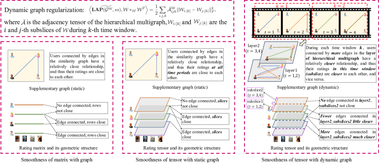
Figure 3: The illustration of different graph smoothness characteristics in matrix case and tensor case with static and dynamic graph, using a movie rating system with social network of users as the example.

Denote $\mathcal{L}:=\mathbf{LAP}(\mathcal{G}^{\mathcal{W}},ss)$ for brevity, then we have

$$\langle\widetilde{\mathcal{L}},\mathcal{W}*_{M}\mathcal{W}^{T}\rangle=\frac{1}{C}\langle\mathcal{L},\widehat{\mathcal{W}*_{M}\mathcal{W}^{T}}\rangle=\frac{1}{C}\langle\mathcal{L},\widehat{\mathcal{W}}\star\widehat{\mathcal{W}}^{T}\rangle.$$

For a matrix $A$, we use $A^{(t)}$ to denote the $t$-th row of $A$, and for a order-3 tensor $\mathcal{A}$, we use $\mathcal{A}^{(t)}$ to denote the $t$-th frontal slice of $\mathcal{A}$. Then $\langle\mathcal{L},\widehat{\mathcal{W}}\star\widehat{\mathcal{W}}^{T}\rangle$ can be written as

$$\langle\mathcal{L},\widehat{\mathcal{W}}\star\widehat{\mathcal{W}}^{T}\rangle=\sum_{t=1}^{T}\langle\mathcal{L}^{(t)},\widehat{\mathcal{W}}^{(t)}(\widehat{\mathcal{W}}^{(t)})^{T}\rangle,$$

and matrices $\widehat{\mathcal{W}}^{(t)}$ have the following formulations:

$$\widehat{\mathcal{W}}^{(t)}=\begin{pmatrix}M^{(t)}\mathcal{W}_{11:}&M^{(t)}\mathcal{W}_{12:}&\cdots&M^{(t)}\mathcal{W}_{1m:}\\ M^{(t)}\mathcal{W}_{21:}&M^{(t)}\mathcal{W}_{22:}&\cdots&M^{(t)}\mathcal{W}_{2m:}\\ \vdots&\vdots&\ddots&\vdots\\ M^{(t)}\mathcal{W}_{m1:}&M^{(t)}\mathcal{W}_{m2:}&\cdots&M^{(t)}\mathcal{W}_{mm:}\end{pmatrix},$$

where $\mathcal{W}_{ij:}\in\mathbb{R}^{1\times 1\times T}$ means the tube fibers of the corresponding tensors. Taking $\mathcal{L}=\vec{\mathcal{D}}^{\mathcal{W}}-\vec{\mathcal{A}}^{\mathcal{W}}$ into consideration, we can obtain that

$$\begin{split}\langle\mathcal{L}^{(t)},\widehat{\mathcal{W}}^{(t)}(\widehat{\mathcal{W}}^{(t)})^{T}\rangle&=\frac{1}{2}\sum_{i,j}\vec{\mathcal{A}}_{ijt}^{\mathcal{W}}\|M^{(t)}\mathcal{W}_{i::}^{T}-M^{(t)}\mathcal{W}_{j::}^{T}\|_{F}^{2},\end{split}$$

where $\mathcal{W}_{i::}$, $\mathcal{W}_{j::}\in\mathbb{R}^{1\times T\times T}$ means the $i$ and $j$-th horizontal slice of $\mathcal{W}$, respectively. With this, we have

$$\begin{split}\langle\widetilde{\mathcal{L}},\mathcal{W}*_{M}\mathcal{W}^{T}\rangle&=\frac{1}{2C}\sum_{i,j,t}\vec{\mathcal{A}}_{ijt}^{\mathcal{W}}\|M^{(t)}\mathcal{W}_{i::}^{T}-M^{(t)}\mathcal{W}_{j::}^{T}\|_{F}^{2}.\end{split}$$

Taking the special structures of $\vec{\mathcal{A}}^{\mathcal{W}}$ and $M$ into consideration, $\langle\widetilde{\mathcal{L}},\mathcal{W}*_{M}\mathcal{W}^{T}\rangle$ can be finally written to the following equivalent form:

$$\begin{split}&\langle\widetilde{\mathcal{L}},\mathcal{W}*_{M}\mathcal{W}^{T}\rangle\\ &=\frac{1}{2C}\sum_{i,j}\sum_{k=1}^{K}\breve{\mathcal{A}}_{ijk}^{\mathcal{W}}\sum_{t\in[k]}\|M^{(t)}_{ss}(\mathcal{W}_{i:[k]}^{T}-\mathcal{W}_{j:[k]}^{T})\|_{F}^{2}\\ &=\frac{1}{2C}\sum_{i,j,k}\breve{\mathcal{A}}_{ijk}^{\mathcal{W}}\|M_{ss}(\mathcal{W}_{i:[k]}^{T}-\mathcal{W}_{j:[k]}^{T})\|_{F}^{2}\\ &=\frac{1}{2C}\sum_{i,j,k}\breve{\mathcal{A}}_{ijk}^{\mathcal{W}}\|\widehat{\mathcal{W}}_{i:[k]}-\widehat{\mathcal{W}}_{j:[k]}\|_{F}^{2}\\ &=\frac{1}{2}\sum_{i,j,k}\breve{\mathcal{A}}_{ijk}^{\mathcal{W}}\|\mathcal{W}_{i:[k]}-\mathcal{W}_{j:[k]}\|_{F}^{2},\end{split}$$ (8)

where $\breve{A}^{\mathcal{W}}$ is the adjacency tensor of hierarchical multigraph, and $\mathcal{W}_{i:[k]}$ is a segment of the horizontal slice $\mathcal{W}_{i::}$ with width $ss$, which can thus be called a subslice.

From (8) we can see that the proposed tensor-oriented graph smoothness regularization (7) is actually equivalent to the sum of products of each entry in the multigraph $\breve{A}^{\mathcal{W}}_{ijk}$ and the distance between corresponding subslices $\mathcal{W}_{i:[k]}$ and $\mathcal{W}_{j:[k]}$, which can be seen as an extension of the matrix case (6). Apparently, lessening (8) forces the distance $\|\mathcal{W}_{i:[k]}-\mathcal{W}_{j:[k]}\|_{F}^{2}$ to be smaller for larger $\breve{A}^{\mathcal{W}}_{ijk}$. Considering that $\breve{A}^{\mathcal{W}}_{ijk}$ means the number of edges between $i$ and $j$-th vertices in $k$-th layer of the hierarchical multigraph, it actually counts the number of time periods in which the two vertices are connected during the $k$-th dynamic subgraph, i.e., the $k$-th time interval. Thus, (7) is a reasonable dynamic graph smoothness regularization encouraging the users with more time-frequent connections during a time interval to be closer with each other in the rating subtensor of corresponding time interval. Here, the length of time intervals can be controlled by similarity scale $ss$ which reflects the level of sophistication for dynamic characterization. Therefore, we can use (7) as a smoothness term to integrally embed the dynamic graph information into tensor $\mathcal{W}$. Meanwhile, it is worth noting that there are two special cases: (1) when $T=1$, tensor $\mathcal{X}$ degenerates into a matrix, and in this case (7) is equivalent to the regularization in matrix case (6); (2) when $T>1$ while $\mathcal{G}^{\mathcal{W}}$ is a static graph, (7) is similar to the matrix case except for the distances computed by the whole slices. In Fig. 3 we intuitively compare the graph smoothness characteristics in matrix case and tensor case with static and dynamic graph.

Based on the proposed tensor-oriented graph smoothness regularization, we can then develop a new model for TC with dynamic graphs as follows. For a TC problem with underlying tensor $\mathcal{X}\in\mathbb{R}^{n_{1}\times n_{2}\times n_{3}}$, partial observations $\mathcal{P}_{\Omega}(\mathcal{X})$, and dynamic graphs $\mathcal{G}^{\mathcal{W}}$, $\mathcal{G}^{\mathcal{H}}$, we can simultaneously exploit the low-rank property and underlying graph structure in a unified model by incorporating regularizer (7) into low-rank model (5), which can be written as:

$$\begin{split}&\check{\mathcal{W}},\check{\mathcal{H}}\\ &=\arg\min_{\mathcal{W},\mathcal{H}}\frac{1}{2}\|\mathcal{P}_{\Omega}(\mathcal{X}-\mathcal{W}*_{M}\mathcal{H}^{T})\|_{F}^{2}+\frac{\lambda_{1}}{2}(\|\mathcal{W}\|_{F}^{2}+\|\mathcal{H}\|_{F}^{2})\\ &+\frac{\lambda_{\mathcal{G}}}{2}(\langle\widetilde{\mathbf{LAP}(\mathcal{G}^{\mathcal{W}},ss)},\mathcal{W}*_{M}\mathcal{W}^{T}\rangle+\langle\widetilde{\mathbf{LAP}(\mathcal{G}^{\mathcal{H}},ss)},\mathcal{H}*_{M}\mathcal{H}^{T}\rangle).\end{split}$$

Given that $\|\mathcal{W}\|_{F}^{2}=\frac{1}{C}\|\widehat{\mathcal{W}}\|_{F}^{2}=\frac{1}{C}\langle\widehat{\mathcal{I}^{\mathcal{W}}},\widehat{\mathcal{W}}\star\widehat{\mathcal{W}}^{T}\rangle=\langle\mathcal{I}^{\mathcal{W}},\mathcal{W}*_{M}\mathcal{W}^{T}\rangle$ and $\|\mathcal{H}\|_{F}^{2}=\langle\mathcal{I}^{\mathcal{H}},\mathcal{H}*_{M}\mathcal{H}^{T}\rangle$, where $\mathcal{I}^{\mathcal{W}}\in\mathbb{R}^{n_{1}\times n_{1}\times n_{3}}$ and $\mathcal{I}^{\mathcal{H}}\in\mathbb{R}^{n_{2}\times n_{2}\times n_{3}}$ denote the identity tensors under $*_{M}$, the model can be further rewritten as:

$$\begin{split}\check{\mathcal{W}},\check{\mathcal{H}}=&\arg\min_{\mathcal{W},\mathcal{H}}\frac{1}{2}\|\mathcal{P}_{\Omega}(\mathcal{X}-\mathcal{W}*_{M}\mathcal{H}^{T})\|_{F}^{2}\\ &+\frac{1}{2}(\langle\mathcal{L}^{\mathcal{W}},\mathcal{W}*_{M}\mathcal{W}^{T}\rangle+\langle\mathcal{L}^{\mathcal{H}},\mathcal{H}*_{M}\mathcal{H}^{T}\rangle),\end{split}$$ (9)

where $\mathcal{L}^{\mathcal{W}}:=\lambda_{\mathcal{G}}\widetilde{\mathbf{LAP}(\mathcal{G}^{\mathcal{W}},ss)}+\lambda_{1}\mathcal{I}^{\mathcal{W}}$, $\mathcal{L}^{\mathcal{H}}:=\lambda_{\mathcal{G}}\widetilde{\mathbf{LAP}(\mathcal{G}^{\mathcal{H}},ss)}+\lambda_{1}\mathcal{I}^{\mathcal{H}}$. (9) is our final model for TC with dynamic graphs.

5 Optimization Algorithm

In this section, we propose an efficient algorithm based on alternating direction method of multiplier (ADMM) and conjugate gradient (CG) to solve the model (9).

5.1 Optimization by ADMM

We introduce three auxiliary variables $\mathcal{A}$, $\mathcal{B}$ and $\mathcal{E}$, and transform model (9) to the following equivalent form:

$$\begin{split}&\min_{\mathcal{W},\mathcal{H},\mathcal{A},\mathcal{B},\mathcal{E}}\frac{1}{2}\|\mathcal{E}-\mathcal{W}*_{M}\mathcal{H}^{T}\|_{F}^{2}\\ &~{}~{}~{}~{}~{}~{}~{}~{}~{}~{}~{}~{}~{}~{}~{}~{}+\frac{1}{2}(\langle\mathcal{L}^{\mathcal{W}},\mathcal{A}*_{M}\mathcal{A}^{T}\rangle+\langle\mathcal{L}^{\mathcal{H}},\mathcal{B}*_{M}\mathcal{B}^{T}\rangle)\\ &~{}\rm{s.t}.~{}\mathcal{A}=\mathcal{W},\mathcal{B}=\mathcal{H},\mathcal{P}_{\Omega}(\mathcal{E})=\mathcal{P}_{\Omega}(\mathcal{X}).\end{split}$$ (10)

The augmented Lagrangian function for (10) is:

$$\begin{split}&L_{A}(\mathcal{W},\mathcal{H},\mathcal{A},\mathcal{B},\mathcal{E})=\frac{1}{2}\|\mathcal{E}-\mathcal{W}*_{M}\mathcal{H}^{T}\|_{F}^{2}\\ &\quad+\frac{1}{2}(\langle\mathcal{L}^{\mathcal{W}},\mathcal{A}*_{M}\mathcal{A}^{T}\rangle+\langle\mathcal{L}^{\mathcal{H}},\mathcal{B}*_{M}\mathcal{B}^{T}\rangle)\\ &\quad+\frac{\beta}{2}\|\mathcal{A}-\mathcal{W}-\frac{\bm{\lambda}^{\mathcal{W}}}{\beta}\|^{2}_{F}+\frac{\beta}{2}\|\mathcal{B}-\mathcal{H}-\frac{\bm{\lambda}^{\mathcal{H}}}{\beta}\|^{2}_{F}\\ &\quad+\frac{\beta}{2}\|\mathcal{P}_{\Omega}(\mathcal{E})-\mathcal{P}_{\Omega}(\mathcal{X})-\mathcal{P}_{\Omega}(\frac{\bm{\lambda}^{\mathcal{E}}}{\beta})\|^{2}_{F},\end{split}$$ (11)

where $\bm{\lambda}^{\mathcal{W}}$, $\bm{\lambda}^{\mathcal{H}}$ and $\bm{\lambda}^{\mathcal{E}}$ are the Lagrange multiplier tensors, and $\beta$ is the positive penalty scalar. Then we can alternatively minimize $L_{A}$ with respect to each variable by the following sub-problems.

5.2 $\mathcal{W},\mathcal{H}$ sub-problem

The sub-problem to optimize $L_{A}$ with respect to $\mathcal{W}$ is:

$$\min_{\mathcal{W}}\frac{\beta}{2}\|\mathcal{A}-\mathcal{W}-\frac{\bm{\lambda}^{\mathcal{W}}}{\beta}\|^{2}_{F}+\frac{1}{2}\|\mathcal{E}-\mathcal{W}*_{M}\mathcal{H}^{T}\|^{2}_{F},$$ (12)

which can be rewritten in the transform domain:

$$\min_{\widehat{\mathcal{W}}}\frac{\beta}{2C}\|\widehat{\mathcal{A}}-\widehat{\mathcal{W}}-\frac{\widehat{\bm{\lambda}^{\mathcal{W}}}}{\beta}\|^{2}_{F}+\frac{1}{2C}\|\widehat{\mathcal{E}}-\widehat{\mathcal{W}}\star\widehat{\mathcal{H}^{T}}\|^{2}_{F}.$$ (13)

Considering the independence of those frontal slices in $\widehat{\mathcal{W}}$, $\widehat{\mathcal{W}}^{(1)},...,\widehat{\mathcal{W}}^{(n_{3})}$ can be solved separately and in parallel. Denote a specific frontal slice $\widehat{\mathcal{W}}^{(t)}$ as $\widehat{W}$, and $\widehat{\mathcal{A}}^{(t)}$ as $\widehat{A}$, $\widehat{\mathcal{E}}^{(t)}$ as $\widehat{E}$, $\widehat{\mathcal{H}^{T}}^{(t)}$ as $\widehat{H}^{T}$, $\widehat{\mathcal{E}}^{(t)}$ as $\widehat{E}$, $\widehat{\bm{\lambda}^{\mathcal{W}}}^{(t)}$ as $\widehat{\bm{\lambda}^{W}}$, then solving $\widehat{W}$ corresponds to the following optimization problem:

$$\min_{\widehat{W}}f(\widehat{W}):=\frac{\beta}{2}\|\widehat{A}-\widehat{W}-\frac{\widehat{\bm{\lambda}^{W}}}{\beta}\|^{2}_{F}+\frac{1}{2}\|\widehat{E}-\widehat{W}\widehat{H}^{T}\|^{2}_{F}.$$ (14)

Optimization problem (14) can be treated as solving the following linear system:

$$\widehat{W}(\widehat{H}^{T}\widehat{H}+\beta I)=\beta\widehat{A}-\widehat{\bm{\lambda}^{W}}+\widehat{E}\widehat{H},$$ (15)

which can be solved by off-the-shelf conjugate gradient techniques. After obtaining $\widehat{\mathcal{W}}$, we can transform back to the original domain to get $\mathcal{W}$. Obviously, $\mathcal{H}$ can be solved in similar way as $\mathcal{W}$, except that (15) should be replaced by

$$\widehat{H}(\widehat{W}^{T}\widehat{W}+\beta I)=\beta\widehat{B}-\widehat{\bm{\lambda}^{H}}+\widehat{E}^{T}\widehat{W}$$ (16)

5.3 $\mathcal{A},\mathcal{B}$ sub-problem

Optimizing $L_{A}$ with respect to $\mathcal{A}$ can be formalized as:

$$\min_{\mathcal{A}}\frac{\beta}{2}\|\mathcal{A}-\mathcal{W}-\frac{\bm{\lambda}^{\mathcal{W}}}{\beta}\|^{2}_{F}+\frac{1}{2}(\langle\mathcal{L}^{\mathcal{W}},\mathcal{A}*_{M}\mathcal{A}^{T}\rangle).$$ (17)

As the $\mathcal{W}$ sub-problem, we can also rewrite (17) in the transform domain, and solve $\widehat{\mathcal{A}}^{(1)},...,\widehat{\mathcal{A}}^{(n_{3})}$ separately and in parallel. Denote a specific frontal slice $\widehat{\mathcal{A}}^{(t)}$ as $\widehat{A}$, and $\widehat{\mathcal{W}}^{(t)}$ as $\widehat{W}$, $(\widehat{\mathcal{L}^{\mathcal{W}}})^{(t)}$ as $\widehat{L^{\mathcal{W}}}$, $(\widehat{\bm{\lambda}^{\mathcal{W}}})^{(t)}$ as $\widehat{\bm{\lambda}^{W}}$, then solving $\widehat{A}$ corresponds to the following optimization problem:

$$\min_{\widehat{A}}g(\widehat{A}):=\frac{\beta}{2}\|\widehat{A}-\widehat{W}-\frac{\widehat{\bm{\lambda}^{W}}}{\beta}\|^{2}_{F}+\frac{1}{2}\langle\widehat{L^{\mathcal{W}}},\widehat{A}\widehat{A}^{T}\rangle,$$ (18)

which is equivalent to the linear system

$$(\widehat{L^{\mathcal{W}}}+\beta I)\widehat{A}=\beta\widehat{W}+\widehat{\bm{\lambda}^{W}}.$$ (19)

We can solve $\mathcal{B}$ in similar way apart from that (19) should be replaced by

$$(\widehat{L^{\mathcal{H}}}+\beta I)\widehat{B}=\beta\widehat{H}+\widehat{\bm{\lambda}^{H}}.$$ (20)

It is worth mentioning that the solving of $\mathcal{A}$ and $\mathcal{B}$ are independent and thus can be implemented in parallel.

5.4 $\mathcal{E}$ sub-problem

The sub-problem to optimize $L_{A}$ with respect to $\mathcal{E}$ has the following form:

$$\min_{\mathcal{E}}\frac{1}{2}\|\mathcal{E}-\mathcal{W}*_{M}\mathcal{H}^{T}\|_{F}^{2}+\frac{\beta}{2}\|\mathcal{P}_{\Omega}(\mathcal{E})-\mathcal{P}_{\Omega}(\mathcal{X})-\mathcal{P}_{\Omega}(\frac{\bm{\lambda}^{\mathcal{E}}}{\beta})\|^{2}_{F}，$$

which has the following explicit solution:

$$\begin{split}\mathcal{E}&=\frac{1}{1+\beta}\mathcal{P}_{\Omega}(\beta\mathcal{X}+\bm{\lambda}^{\mathcal{E}}+\mathcal{W}*_{M}\mathcal{H}^{T})+\mathcal{P}_{\bar{\Omega}}(\mathcal{W}*_{M}\mathcal{H}^{T}),\end{split}$$ (21)

where $\bar{\Omega}$ is the orthogonal complement of $\Omega$.

5.5 Updating Multipliers

Finally, the multipliers associated with $L_{A}$ are updated by the following formulas:

$$\left\{\begin{array}[]{l}\bm{\lambda}^{\mathcal{W}}\leftarrow\bm{\lambda}^{\mathcal{W}}-\gamma\beta(\mathcal{A}-\mathcal{W})\\ \bm{\lambda}^{\mathcal{H}}\leftarrow\bm{\lambda}^{\mathcal{H}}-\gamma\beta\big{(}\mathcal{B}-\mathcal{H})\\ \bm{\lambda}^{\mathcal{E}}\leftarrow\bm{\lambda}^{\mathcal{E}}-\gamma\beta(\mathcal{P}_{\Omega}(\mathcal{E})-\mathcal{P}_{\Omega}(\mathcal{X}))\end{array}\right.$$ (22)

where $\gamma$ is a parameter associated with convergence rate of the algorithm.

Based on the above descriptions, the proposed algorithm for model (9) can now be summarized in Algorithm 1.

Algorithm 1 Optimization Algorithm for the Model (9)

0:  observed tensor $\mathcal{P}_{\Omega}(\mathcal{X})\in\mathbb{R}^{n_{1}\times n_{2}\times n_{3}}$; dynamic graphs $\mathcal{G}^{\mathcal{W}},\mathcal{G}^{\mathcal{H}}$; similarity scale $ss$; transform matrix $\mathbf{M}$; rank $r$, parameters $\lambda_{\mathcal{G}}$, $\lambda_{1}$.

0:  Initial $\mathcal{W}=\mbox{randn}(n_{1},r,n_{3})$, $\mathcal{H}=\mbox{randn}(n_{2},r,n_{3})$, $\mathcal{A}=\mathcal{W}$, $\mathcal{B}=\mathcal{H}$, $\mathcal{E}=\mathcal{P}_{\Omega}(\mathcal{X})$.

1:  while not converge do

2:     Update $\mathcal{W}$ via Eq.(15).

3:     Update $\mathcal{H}$ via Eq.(16);

4:     Update $\mathcal{A}$, $\mathcal{B}$ via Eq.(19) and (20), respectively;

5:     Update $\mathcal{E}$ via Eqs.(21).

6:     Update multipliers via Eqs.(22).

7:  end while

7:  The reconstructed tensor $\mathcal{X}=\mathcal{W}*_{M}\mathcal{H}^{T}$.

5.6 Complexity Analysis

Here we analyze the computational complexity of Algorithm 1. We employ Discrete Fourier Transformation (DFT) as the transform in t-SVD, which has demonstrated superiority in many t-SVD related works [51, 21], and thus the computational cost for transforming a $n_{1}\times n_{2}\times n_{3}$ tensor is $O(n_{1}n_{2}n_{3}\log{n_{3}})$. At each iteration, the main cost of Algorithm 1 lies in the subproblems (15), (16), (19), (20) and (21). Solving (15) mainly involves the tensor DFT and conjugate gradient method. It is known that the computational cost of conjugate gradient method for solving a linear system $A\mathbf{x}=\mathbf{b}$ is $O(N\sqrt{K})$, where $N$ is the number of nonzero entries in $A$ and $K$ is its condition number. Thus the main cost solving (15) is $O(r^{2}\sqrt{K_{1}}+n_{1}n_{2}n_{3}\log{n_{3}})$, where $K_{1}$ is the condition numbers for the linear systems. Similarly, the cost solving (16), (19), (20) is $O(r^{2}\sqrt{K_{2}}+n_{1}n_{2}n_{3}\log{n_{3}})$, $O(n_{1}^{2}\sqrt{K_{3}}+n_{1}^{2}n_{3}\log{n_{3}})$, and $O(n_{2}^{2}\sqrt{K_{4}}+n_{2}^{2}n_{3}\log{n_{3}})$, respectively, where $K_{2}$, $K_{3}$, $K_{4}$ are corresponding condition number. As for subproblem (21), the main computation lies in the tensor t-product and tensor DFT, thus its cost is $O(rn_{1}n_{2}n_{3}+r(n_{1}+n_{2})n_{3}\log{n_{3}})$. In all, the computational complexity of Algorithm 1 is $O(r^{2}\sqrt{K_{1}}+r^{2}\sqrt{K_{2}}+n_{1}^{2}\sqrt{K_{3}}+n_{2}^{2}\sqrt{K_{4}}+rn_{1}n_{2}n_{3}+((n_{1}+n_{2})^{2}+r(n_{1}+n_{2}))n_{3}\log{n_{3}})$. Considering that condition numbers could not be very large and $n_{1}$, $n_{2}$ are usually not very different, the cost can be further simplified as $O(rn_{1}n_{2}n_{3}+n_{1}n_{2}n_{3}\log{n_{3}})$.

In Table I, we compare the computational complexity of our method with some representative TC methods, including three matricization methods SiLRTC [43], Tmac [60], RMTC [61], and two tensor modeling methods TNN [49], Alt-Min [62], where $r_{1}$, $r_{2}$ and $r_{3}$ denote the rank of the three unfolded matrices in matricization methods, respectively. From Table I we can see that our method outperforms the compared ones on computational efficiency.

TABLE I: Comparison of computational complexities of some representative TC methods.

Method	Computational complexity
SiLRTC	$O((n_{1}+n_{2}+n_{3})n_{1}n_{2}n_{3})$
Tmac	$O((r_{1}+r_{2}+r_{3})n_{1}n_{2}n_{3})$
RMTC	$O(r_{1}r_{2}r_{3}n_{1}n_{2}n_{3})$
TNN	$O(\min(n_{1},n_{2})n_{1}n_{2}n_{3}+n_{1}n_{2}n_{3}\log{n_{3}})$
Alt-Min	$O(r(n_{1}+n_{2})n_{3}\log{n_{3}}+rn_{1}n_{2}n_{3}^{2}\log^{2}(\max(n_{1},n_{2}))$
Ours	$O(rn_{1}n_{2}n_{3}+n_{1}n_{2}n_{3}\log{n_{3}})$

5.7 Convergence Analysis

Denote the objective function of the optimization problem (10) as

$$\begin{split}&F(\mathcal{W},\mathcal{H},\mathcal{A},\mathcal{B},\mathcal{E})=\frac{1}{2}\|\mathcal{E}-\mathcal{W}*_{M}\mathcal{H}^{T}\|_{F}^{2}\\ &~{}~{}~{}~{}~{}~{}~{}~{}~{}~{}~{}~{}~{}~{}~{}~{}+\frac{1}{2}(\langle\mathcal{L}^{\mathcal{W}},\mathcal{A}*_{M}\mathcal{A}^{T}\rangle+\langle\mathcal{L}^{\mathcal{H}},\mathcal{B}*_{M}\mathcal{B}^{T}\rangle),\end{split}$$ (23)

and denote the sequence generated by Algorithm 1 as $(\mathcal{W}^{k},\mathcal{H}^{k},\mathcal{A}^{k},\mathcal{B}^{k},\mathcal{E}^{k})$, then we can give the following convergence result of Algorithm 1.

Theorem 1:

If $\beta>r^{2}(n_{1}+n_{2})n_{3}(\text{Trace}(\overline{\mathcal{L}^{\mathcal{W}}})+\text{Trace}(\overline{\mathcal{L}^{\mathcal{H}}}))$, then the bounded sequence $(\mathcal{W}^{k},\mathcal{H}^{k},\mathcal{A}^{k},\mathcal{B}^{k},\mathcal{E}^{k})$ generated by Algorithm 1 satisfies the following properties:
(1). Objective $F(\mathcal{W}^{k},\mathcal{H}^{k},\mathcal{A}^{k},\mathcal{B}^{k},\mathcal{E}^{k})$ converges as $k\rightarrow\infty$.
(2). The sequence $(\mathcal{W}^{k},\mathcal{H}^{k},\mathcal{A}^{k},\mathcal{B}^{k},\mathcal{E}^{k})$ has at least a limit point $(\mathcal{W}^{*},\mathcal{H}^{*},\mathcal{A}^{*},\mathcal{B}^{*},\mathcal{E}^{*})$, and any limit point $(\mathcal{W}^{*},\mathcal{H}^{*},\mathcal{A}^{*},\mathcal{B}^{*},\mathcal{E}^{*})$ is a feasible Nash point of the objective $F$.
(3). For the sequence $(\mathcal{W}^{k},\mathcal{H}^{k},\mathcal{A}^{k},\mathcal{B}^{k},\mathcal{E}^{k})$, define $u_{k}=\min_{0\leq l\leq k}(\|\mathcal{A}^{l+1}-\mathcal{A}^{l}\|_{2}^{2}+\|\mathcal{B}^{l+1}-\mathcal{B}^{l}\|_{2}^{2}+\|\mathcal{W}^{l+1}-\mathcal{W}^{l}\|_{2}^{2}+\|\mathcal{H}^{l+1}-\mathcal{H}^{l}\|_{2}^{2}+\|\mathcal{P}_{\Omega}(\mathcal{E}^{l+1}-\mathcal{E}^{l})\|_{2}^{2})$, then the convergence rate of $u_{k}$ is $o(1/k)$.

The proof of Theorem 1 can be found in Section 1 of the supplementary material.

Theorem 1 gives the theoretical convergence guarantee and convergence rate which states that the proposed ADMM can achieve a sublinear convergence rate of $o(1/k)$, despite the nonconvex and complex nature of our model. Furthermore, we also provide an empirical analysis to support the good convergence behavior of Algorithm 1. We showcase the convergence curves in Section 6 of the supplementary material due to the page limitation, which validates the convergence performance of Algorithm 1.

6 Theoretical Analysis

In this section, we provide statistical analysis of the proposed dynamic graph regularized low-rank TC model. To this end, we first demonstrate that the proposed graph smoothness regularization is actually equivalent to a weighted tensor nuclear norm, where the weights implicitly characterize the graph information. This equivalence will facilitate our subsequent theoretical analysis on the graph regularized low-rank tensor estimators.

6.1 Equivalence to A Weighted Tensor Nuclear Norm

In order to showcase the alignment between the proposed graph smoothness regularization and a weighted tensor nuclear norm, we utilize a tensor atomic norm as a conduit. To this end, we first generalize the definition of weighted atomic norm of matrices to the tensor case. Let $M\in\mathbb{R}^{T\times T}$ be a invertible linear transform matrix with $MM^{T}=M^{T}M=CI$, and $\mathcal{P}=[\mathcal{P}_{:1:},\mathcal{P}_{:2:},...,\mathcal{P}_{:m:}]\in\mathbb{R}^{m\times m\times T}$ a basis of lateral slice space $\mathbb{R}^{m\times 1\times T}$ under transform matrix $M$, i.e., each lateral slice $\mathcal{W}\in\mathbb{R}^{m\times 1\times T}$ can be expressed as a linear combination $\mathcal{W}=\mathcal{P}*_{M}\mathcal{U}$ with representation $\mathcal{U}\in\mathbb{R}^{m\times 1\times T}$ and $\|U\|_{F}=1$. Meanwhile, let $\mathcal{S}_{\mathcal{P}}\in\mathbb{R}^{m\times m\times T}$ be a f-diagonal tensor with $(\mathcal{S}_{\mathcal{P}})_{ii:}\geq 0,i=1,2,...,m$ encoding the weight of basis $\mathcal{P}$ spanning the space. Obviously, tensor $\mathcal{P}*_{M}\mathcal{S}_{\mathcal{P}}$ is also a basis. Similarly, let $\mathcal{Q}=[\mathcal{Q}_{:1:},\mathcal{Q}_{:2:},...,\mathcal{Q}_{:n:}]\in\mathbb{R}^{n\times n\times T}$ and $\mathcal{S}_{\mathcal{Q}}\in\mathbb{R}^{n\times n\times T}$ be the basis and corresponding weight tensor for space $\mathbb{R}^{n\times 1\times T}$ under transform matrix $M$. Denote $\mathcal{A}=\mathcal{P}*_{M}\mathcal{S}_{\mathcal{P}}$ and $\mathcal{B}=\mathcal{Q}*_{M}\mathcal{S}_{\mathcal{Q}}$, and we can then define a weighted tensor atomic set as follows:

$$\begin{split}\mathscr{A}:=\{\mathcal{D}=\mathcal{W}*_{M}\mathcal{H}^{T}:&\mathcal{W}=\mathcal{A}*_{M}\mathcal{U},\mathcal{H}=\mathcal{B}*_{M}\mathcal{V},\\ &\|\mathcal{U}\|_{F}=\|\mathcal{V}\|_{F}=1\}.\end{split}$$ (24)

Then we can introduce the following definition:

Definition 10 (weighted tensor atomic norm):

Given a tensor $\mathcal{X}\in\mathbb{R}^{m\times n\times T}$, its weighted tensor atomic norm corresponding to the atomic set $\mathscr{A}$ is defined as:

$$\|\mathcal{X}\|_{\mathscr{A}}:=\text{inf}\sum_{\mathcal{D}_{i}\in\mathscr{A}}\lvert d_{i}\rvert,~{}~{}\text{s.t.}~{}\mathcal{X}=\sum_{\mathcal{D}_{i}\in\mathscr{A}}d_{i}\mathcal{D}_{i}.$$ (25)

Based on those definitions, we can prove the following result:

Theorem 2:

For any $\mathcal{A}=\mathcal{P}*_{M}\mathcal{S}_{\mathcal{P}}$ and $\mathcal{B}=\mathcal{Q}*_{M}\mathcal{S}_{\mathcal{Q}}$, and the corresponding weighted atomic set $\mathscr{A}$, the following equality holds:

$$\begin{split}\|\mathcal{X}\|_{\mathscr{A}}&=\mathop{\rm inf}_{\mathcal{W},\mathcal{H}}\frac{1}{2}\{\|\mathcal{A}^{-1}*_{M}\mathcal{W}\|_{F}^{2}+\|\mathcal{B}^{-1}*_{M}\mathcal{H}\|_{F}^{2}\}\\ &~{}~{}\text{s.t.}~{}\mathcal{X}=\mathcal{W}*_{M}\mathcal{H}^{T}.\end{split}$$ (26)

The proof of the above theorem is placed in Section 2 of the supplementary material.

Theorem 2 gives an equivalent form of the atomic norm (25), based on which in the following we can show that the regularizer in our model (9) is actually a weighted tensor atomic norm. Let $\mathcal{L}^{\mathcal{W}}=\mathcal{U}_{\mathcal{W}}*_{M}\mathcal{S}_{\mathcal{W}}*_{M}\mathcal{U}_{\mathcal{W}}^{T}$ and $\mathcal{L}^{\mathcal{H}}=\mathcal{U}_{\mathcal{H}}*_{M}\mathcal{S}_{\mathcal{H}}*_{M}\mathcal{U}_{\mathcal{H}}^{T}$ be the tensor eigen decomposition for tensors $\mathcal{L}^{\mathcal{W}}$ and $\mathcal{L}^{\mathcal{H}}$, then we have:

$$\begin{split}\langle\mathcal{L}^{\mathcal{W}},\mathcal{W}*_{M}\mathcal{W}^{T}\rangle&=\frac{1}{C}\langle\overline{\mathcal{L}^{\mathcal{W}}},\overline{\mathcal{W}}~{}\overline{\mathcal{W}}^{T}\rangle\\ &=\frac{1}{C}\langle\overline{\mathcal{U}_{\mathcal{W}}}~{}\overline{\mathcal{S}_{\mathcal{W}}}~{}\overline{\mathcal{U}_{\mathcal{W}}}^{T},\overline{\mathcal{W}}~{}\overline{\mathcal{W}}^{T}\rangle.\end{split}$$

We define $\mathcal{A}=\mathcal{U}_{\mathcal{W}}*_{M}\mathcal{S}_{\mathcal{W}}^{-1/2}$ to conform to the form in Theorem 2 then $\mathcal{A}^{-1}=\mathcal{S}_{\mathcal{W}}^{1/2}*_{M}\mathcal{U}_{\mathcal{W}}^{T}$, $\overline{\mathcal{A}}=\overline{\mathcal{U}_{\mathcal{W}}}~{}\overline{\mathcal{S}_{\mathcal{W}}}^{-1/2}$, $\overline{\mathcal{A}^{-1}}=\overline{\mathcal{S}_{\mathcal{W}}}^{1/2}~{}\overline{\mathcal{U}_{\mathcal{W}}}^{T}$, and $\overline{\mathcal{U}_{\mathcal{W}}}~{}\overline{\mathcal{S}_{\mathcal{W}}}~{}\overline{\mathcal{U}_{\mathcal{W}}}^{T}=\overline{\mathcal{A}^{-1}}^{T}~{}\overline{\mathcal{A}^{-1}}$. Then $\langle\mathcal{L}^{\mathcal{W}},\mathcal{W}*_{M}\mathcal{W}^{T}\rangle$ can further be written as

$$\begin{split}\langle\mathcal{L}^{\mathcal{W}},\mathcal{W}*_{M}\mathcal{W}^{T}\rangle&=\frac{1}{C}\langle\overline{\mathcal{A}^{-1}}^{T}~{}\overline{\mathcal{A}^{-1}},\overline{\mathcal{W}}~{}\overline{\mathcal{W}}^{T}\rangle\\ &=\frac{1}{C}\|\overline{\mathcal{A}^{-1}}~{}\overline{\mathcal{W}}\|_{F}^{2}=\|\mathcal{A}^{-1}*_{M}\mathcal{W}\|_{F}^{2}.\end{split}$$

Similarly, denote $\mathcal{B}=\mathcal{U}_{\mathcal{H}}*_{M}\mathcal{S}_{\mathcal{H}}^{-1/2}$, then we have $\langle\mathcal{L}^{\mathcal{H}},\mathcal{H}*_{M}\mathcal{H}^{T}\rangle=\|\mathcal{B}^{-1}*_{M}\mathcal{H}\|_{F}^{2}$ . Based on Theorem 2, it can be verified that the regularizer in model (9) is equivalent to a weighted tensor atomic norm (25) with basis tensors $\mathcal{U}_{\mathcal{W}}$, $\mathcal{U}_{\mathcal{H}}$ and the corresponding weight tensors $\mathcal{S}_{\mathcal{W}}^{-1/2}$, $\mathcal{S}_{\mathcal{H}}^{-1/2}$, respectively.

In the above, we demonstrate that the regularizer in our model (9) is equivalent to a weighted tensor atomic norm. Then we introduce two lemmas to show that the defined weighted tensor atomic norm (25) is actually a weighted tensor nuclear norm, and consequently the equivalence between the regularizer in model (9) and the weighted tensor nuclear norm can be directly obtained. Given two weight tensors $\mathcal{A}$ and $\mathcal{B}$, we can define a weighted tensor spectral norm of a tensor $\mathcal{X}$ as $\|\mathcal{X}\|_{\mathcal{A},\mathcal{B}}:=\|\mathcal{A}^{T}*_{M}\mathcal{X}*_{M}\mathcal{B}\|$, based on which we introduce two lemmas.

Lemma 1:

The dual norm of the weighted tensor spectral norm for a tensor $\mathcal{X}$ is a weighted tensor nuclear norm:

$$\|\mathcal{X}\|_{\mathcal{A},\mathcal{B}}^{*}=\|\mathcal{A}^{-1}*_{M}\mathcal{X}*_{M}\mathcal{B}^{-T}\|_{*}.$$

Lemma 2:

For $\mathcal{A}=\mathcal{U}_{\mathcal{W}}*_{M}\mathcal{S}_{\mathcal{W}}^{-1/2}$ and $\mathcal{B}=\mathcal{U}_{\mathcal{H}}*_{M}\mathcal{S}_{\mathcal{H}}^{-1/2}$, and the corresponding weighted atomic set $\mathscr{A}$, the dual norm of the weighted tensor atomic norm for a tensor $\mathcal{X}$ is a weighted tensor spectral norm:

$$\begin{split}\|\mathcal{X}\|_{\mathscr{A}}^{*}&=\|\mathcal{X}\|_{\mathcal{A},\mathcal{B}}=\|\mathcal{A}^{T}*_{M}\mathcal{X}*_{M}\mathcal{B}\|\\ &=\|\mathcal{S}_{\mathcal{W}}^{-1/2}*_{M}\mathcal{U}_{\mathcal{W}}^{T}*_{M}\mathcal{X}*_{M}\mathcal{U}_{\mathcal{H}}*_{M}\mathcal{S}_{\mathcal{H}}^{-1/2}\|.\end{split}$$

The proof of Lemma 1 and Lemma 2 can be found in Section 3 and 4 of the supplementary material, respectively.

From the two lemmas, it is straightforward to say that the defined weighted tensor atomic norm (25) is actually a weighted tensor nuclear norm:

$$\begin{split}\|\mathcal{X}\|_{\mathscr{A}}=\|\mathcal{A}^{-1}*_{M}\mathcal{X}*_{M}\mathcal{B}^{-T}\|_{*}.\end{split}$$ (27)

As a direct corollary, the regularizer in model (9) is also equivalent to the above weighted tensor nuclear norm, where the graph information is implicitly characterized in the weight tensors $\mathcal{A}=\mathcal{U}_{\mathcal{W}}*_{M}\mathcal{S}_{\mathcal{W}}^{-1/2}$ and $\mathcal{B}=\mathcal{U}_{\mathcal{H}}*_{M}\mathcal{S}_{\mathcal{H}}^{-1/2}$.

6.2 Main Theorem

Based on the above conclusions, we then establish statistical consistency guarantees of the proposed dynamic graph regularized low-rank TC model. We first make some assumptions and reformulate the problem. We assume that the true tensor $\mathcal{X}^{*}\in\mathbb{R}^{m\times n\times T}$ is low rank with tubal rank $r^{*}\ll\text{min}\{m,n\}$. We denote the total number of entries in $\mathcal{X}^{*}$ as $D=m\times n\times T$, and suppose that there are totally $N\ll D$ noisy observations $y_{1},y_{2},...,y_{N}$ uniformly sampled from the following observation model:

$$y_{k}=\langle\mathcal{X}^{*},\mathfrak{X}_{k}\rangle+\sigma\xi_{k},k=1,2,...,N,$$ (28)

where $\mathfrak{X}_{k}\in\mathbb{R}^{m\times n\times T}$ are i.i.d random design tensors drawn from uniform distribution on the set $\{\mathbf{e}_{i}\otimes\mathbf{e}_{j}\otimes\mathbf{e}_{t}:\forall i=1,...,m;j=1,...,n;t=1,...,T\}$ with $\otimes$ the outer product operator and $\mathbf{e}_{i}$ the $i$-th standard basis of the corresponding coordinate vector space; random noise $\xi_{k}\in\mathbb{R}$ are independent and centered sub-exponential variables with unit variance, and $\sigma$ is a parameter denoting the variance of noise in the observation. In order to specify the observation model in vector form, denote $\bm{y}\in\mathbb{R}^{N}$ and $\bm{\xi}\in\mathbb{R}^{N}$ as the observation and noise vectors, respectively, i.e., $\bm{y}=[y_{1},y_{2},...,y_{N}]^{T},\bm{\xi}=[\xi_{1},\xi_{2},...,\xi_{N}]^{T}$, and meanwhile define a linear operator $\mathscr{X}(\cdot):\mathbb{R}^{m\times n\times T}\rightarrow\mathbb{R}^{N}$ via

$$\mathscr{X}(\mathcal{X})_{k}=\langle\mathcal{X},\mathfrak{X}_{k}\rangle,k=1,2,...,N,\forall\mathcal{X}\in\mathbb{R}^{m\times n\times T}.$$

With those notations, we can then rewrite the observation model (28) in vectorized form as

$$\bm{y}=\mathscr{X}(\mathcal{X^{*}})+\sigma\bm{\xi}.$$ (29)

For the given $\mathcal{L}^{\mathcal{W}}$ and $\mathcal{L}^{\mathcal{H}}$, let $\mathcal{A}$, $\mathcal{B}$ be the corresponding weight tensors defined in Section 6.1, we then define a graph based complexity measure as

$$\alpha:=\|\mathcal{A}^{-1}*_{M}\mathcal{X}^{*}*_{M}\mathcal{B}^{-T}\|_{\infty}.$$

Based on the vectorized formulation (29) and the equivalence between the regularizer in our model and weighted tensor nuclear norm, our model (9) can then be equivalently reformulated as the following M-estimator:

$$\check{\mathcal{X}}=\arg\min_{\text{rank}(\mathcal{X})\leq r^{*}}\frac{1}{2N}\|\bm{y}-\mathscr{X}(\mathcal{X})\|_{2}^{2}+\lambda\|\mathcal{A}^{-1}*_{M}\mathcal{X}*_{M}\mathcal{B}^{-T}\|_{*},$$ (30)

where $\lambda>0$ is the regularization parameter. We then analyze the statistical performance of estimator (30).

We first introduce a shorthand $d=(m+n)T$ for brevity, and then a non-asymptotic upper bound on the Frobenius norm error is established in the following theorem.

Theorem 3:

Suppose that we observe $N$ entries from tensor $\mathcal{X}^{*}\in\mathbb{R}^{m\times n\times T}$ under observation model $(\ref{observation model 2})$, $\mathcal{X}^{*}$ has rank at most $r^{*}$ with complexity measure $\alpha$. Let $\check{\mathcal{X}}$ be the minimizer of the convex estimator (30) with $\lambda\geq c_{0}\sigma\sqrt{\frac{\log d}{Nn}}$, then we have

$$\frac{\|\check{\mathcal{X}}-\mathcal{X}^{*}\|_{F}^{2}}{D}\leq\alpha^{2}c_{1}\max\left\{\max\{\sigma^{2},1\}\cdot\frac{r^{*}mT\log d}{N},\frac{n\log d}{N}\right\}.$$ (31)

with high probability, where $c_{0}$, $c_{1}$ are positive constants.

The proof of Theorem 3 can be found in Section 5 of the supplementary material.

Theorem 3 guarantees that the per-entry estimation error of our model satisfies

$$\frac{\|\check{\mathcal{X}}-\mathcal{X}^{*}\|_{F}^{2}}{mnT}\lesssim\frac{r^{*}mT\log\left((m+n)T\right)}{N}$$ (32)

with high probability, where $\lesssim$ means that the inequality holds up to a multiplicative constant. Equivalently, it can be seen that with sample complexity $O(r^{*}mT\log\left((m+n)T\right))$, the per-entry estimation error will be small. Then we explain the main differences in the proof, and compare the error bound and sample complexity in Theorem 3 with its two degenerated models (graph-agnostic version and static version) and previous results, by the following remarks.

Remark 1. To proof Theorem 3, we establish a new constraint set and corresponding restricted strong convexity for weighted tensors, and also demonstrate the decomposability of the weighted error tensor. Furthermore, we upper bound the distance between the error tensor and weighted error tensor based on Talagrand’s concentration inequality. These constitute the main differences in our proof.

Remark 2. By setting $\textbf{LAP}(\mathcal{G}^{\mathcal{W}})=\textbf{LAP}(\mathcal{G}^{\mathcal{H}})=\mathbf{0}$, i.e., $\mathcal{A}=\mathcal{B}=\mathcal{I}$, in our model (9), we can get a degenerated model without considering the graph information (graph-agnostic model), in which case the corresponding error bound in Theorem 3 could have $\alpha$ replaced by $\alpha^{*}:=\|\mathcal{X}^{*}\|_{\infty}$. In general, it is hard to quantify the relationship between $\alpha$ and $\alpha^{*}$. However, we can empirically demonstrate below by simulations that for informative graphs $\mathcal{G}^{\mathcal{W}}$ and $\mathcal{G}^{\mathcal{H}}$, $\alpha$ is much smaller than $\alpha^{*}$, then the error bound of original model (9) is smaller than the degenerated one. We show the experimental settings in the Section 7 of supplementary material due to page limitations, and plot the corresponding $\alpha^{*}/\alpha$ in Fig. 4 (a). From Fig. 4 (a) we can see that the perfect graph has the largest $\alpha^{*}/\alpha$, and the ratio decreases as the disturbance in the graph increases. When the disturbance is particularly large, it can be seen that $\alpha^{*}/\alpha<1$, in which case the graph is actually uninformative. In Fig. 4 (b) we further compare the relative recovery errors of the graph-agnostic and original graph model, which shows that our original model can achieve smaller recovery errors than the graph-agnostic one, and the more informative graphs (i.e., the smaller $\alpha$) lead to the smaller errors, which is consistent with the conclusion of Theorem 3. Furthermore, the error bound and sample complexity of the graph-agnostic model are in consistence with the previous works on TC, e.g., [63, 64], thus our model can achieve smaller error bound and sample complexity than the previous works, which provides a theoretical guarantee for the superiority of our model.

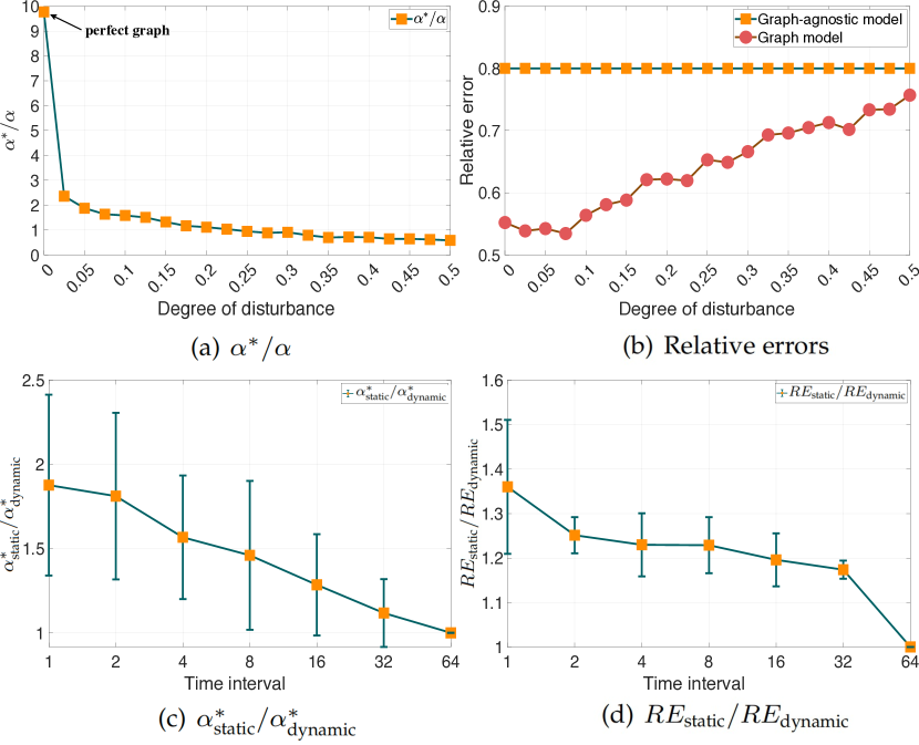
Figure 4: (a)(b) $\alpha^{*}/\alpha$ and relative recovery errors curves with respect to the degrees of perturbation in the graphs. (c)ratios of $\alpha^{*}$ of the static version to original dynamic model under graphs with various time intervals; (d) the corresponding ratios of relative errors.

Remark 3. By directly setting $ss=T$ in our model (9), we can get a degenerated model which exploits the similarities between the whole slices of the tensor. This model cannot accommodate the different degrees of graph dynamism, and also fails to distinguish the edges that connect the same individuals but appear at different time periods, and thus can be seen as a static version of our model. To compare the $\alpha^{*}$ of the static version and our original dynamic model, we denote their corresponding $\alpha^{*}$ as $\alpha^{*}_{\text{static}}$ and $\alpha^{*}_{\text{dynamic}}$, respectively. We generate random tensors with size $50\times 50\times 64$ and corresponding dynamic graphs with various time intervals, the small time interval reflecting the more severe dynamics. For each time interval, we compute the $\alpha^{*}$ and recovery relative error (RE) of the static model and dynamic model with $ss$ equaling to the time interval, respectively. We plot the curves of $\frac{\alpha^{*}_{\text{static}}}{\alpha^{*}_{\text{dynamic}}}$ and $\frac{RE_{\text{static}}}{RE_{\text{dynamic}}}$ with respect to the time intervals in Fig 4 (c) and (d). From Fig 4 (c) we can see that $\frac{\alpha^{*}_{\text{static}}}{\alpha^{*}_{\text{dynamic}}}\geq 1$ and it increases as time interval decreases, which theoretically verifies the superiority of the dynamic model, especially in the scenarios with severe graph dynamism. The $\frac{RE_{\text{static}}}{RE_{\text{dynamic}}}$ curve in Fig 4 (d) also supports this point.

Remark 4. When $T=1$, our bound (32) for TC degenerates to a MC bound, i.e., for a underlying matrix $X\in\mathbf{R}^{m\times n}$ with rank $r*$, the per-entry estimation error satisfies

$$\frac{\|\check{X}-X^{*}\|_{F}^{2}}{mn}\lesssim\frac{r^{*}m\log\left(m+n\right)}{N}$$

with high probability, which is consistent with the results of MC related works [37, 65, 66, 67].

7 Numerical Experiments

Within this section, we assess the efficacy of the introduced algorithm via a sequence of experiments conducted on synthetic and real datasets. These evaluations involve a comparison against several cutting-edge MC and TC techniques. The methods under scrutiny include GRMC[39] and GNIMC[68] for MC, along with LRTC[43], TTC[69], TRNNM[70], TNN[52], and GRTC[59] for TC. The detailed information of those compared methods are listed in TABLE II, including their applicable data structure, employed matrix/tensor decomposition methods, whether the algorithms can deal with side information and whether the algorithms have theoretical guarantees. All the numerical experiments are implemented on a desktop computer with Intel Core i9-9900k, 3.60 GHz, 64.0G RAM and MATLAB R2022a.

TABLE II: Summary of Some Representative MC/TC Models

Algorithm	Data	Decomposition	Side	Theoretical
	Structure	Method	Information	Guarantee
GRMC	Matrix	SVD	Static Graph	Yes
GNIMC	Matrix	SVD	Feature Matrix	Yes
LRTC	Tensor	Tucker	No	No
TTC	Tensor	Tensor Train	No	No
TRNNM	Tensor	Tensor Ring	No	Yes
TNN	Tensor	t-SVD	No	Yes
GRTC	Tensor	CP	Static Graph	No
OURS	Tensor	t-SVD	Dynamic Graph	Yes

7.1 Synthetic Data

In this subsection we examine the performance of the proposed method on synthetic low rank tensors with dynamic graph information. To this end, we first introduce how to generate dynamic graphs with varying degrees of dynamism, and the corresponding low rank tensors with similarities in accordance with the graphs.

7.1.1 Generating Dynamic Graphs

In order to simulate the real dynamic graph such as social network, we should pay attention to its two main properties, i.e., activeness and community structure. For the former, in an active network the social relationships can change frequently, and on the contrary in a introverted network the social relationships can be relatively stable. In the corresponding dynamic graph, the activeness of social network can be reflected by the degree of dynamism: the more dynamic, the more frequently edges change. For the latter, social networks tend to have a distinct community structure (clustering) [71], i.e., some people with similar characteristics (such as common location, interests, occupation, etc) will gather closely to form a relatively independent community group. The connections within a community are quite close, while the inter-community is relatively distant.

With that in mind, we generate a dynamic graph ($m$ vertexes and $T$ time periods) with specific degree of dynamism in the following way. We assume that the dynamic graph changes every certain time interval, and use the length of time interval to control the degree of dynamism: the shorter the time interval, the more dynamic the graph is. Furthermore, to reflect the community structure, for each time interval we randomly generate a graph with totally $m$ vertexes equally divided into $d$ groups by the prototypical graph model ”Community” using GSPbox  [72].

7.1.2 Generating Low Rank Tensors with Dynamic Graphs

Based on the above strategy, we can generate two synthetic dynamic graphs: $\mathcal{G}^{\mathcal{W}}$ with $m$ vertexes and $T$ time periods, and $\mathcal{G}^{\mathcal{H}}$ with $n$ vertexes and also $T$ time periods. Then, we can generate a $m\times n\times T$ tensor with low tubal rank $r$ and graph information $\mathcal{G}^{\mathcal{W}}$, $\mathcal{G}^{\mathcal{H}}$ along its first and second order, respectively, in the following way. We employ Discrete Fourier transform (DFT) [29] as the invertible linear transform $M$, and first generate a random tubal rank $r$ tensor $\mathcal{Z}$ as: $\mathcal{Z}=\mathcal{P}*_{M}\mathcal{Q}^{T}$, where $\mathcal{P}\in\mathbb{R}^{m\times r\times T}$ and $\mathcal{Q}\in\mathbb{R}^{n\times r\times T}$ are independently sampled from Gaussian distribution. Then for each frontal slice of $\mathcal{Z}$, we can embed the row-wise and column-wise similarities based on the corresponding static graphs of $\mathcal{G}^{\mathcal{W}}$and $\mathcal{G}^{\mathcal{H}}$, respectively. Suppose $\textbf{LAP}(\mathcal{G}^{\mathcal{W}})$ and $\textbf{LAP}(\mathcal{G}^{\mathcal{H}})$ are the Laplacian tensors of graphs $\mathcal{G}^{\mathcal{W}}$ and $\mathcal{G}^{\mathcal{H}}$, respectively. Let $\textbf{LAP}(\mathcal{G}^{\mathcal{W}})=\mathcal{U}_{\mathcal{W}}*_{I}\mathcal{S}_{\mathcal{W}}*_{I}\mathcal{U}_{\mathcal{W}}^{T}$, $\textbf{LAP}(\mathcal{G}^{\mathcal{H}})=\mathcal{U}_{\mathcal{H}}*_{I}\mathcal{S}_{\mathcal{H}}*_{I}\mathcal{U}_{\mathcal{H}}^{T}$ are the tensor singular value decomposition of $\textbf{LAP}(\mathcal{G}^{\mathcal{W}})$ and $\textbf{LAP}(\mathcal{G}^{\mathcal{H}})$ under the identity matrix $I$. Then a low rank tensor $\mathcal{X}$ with graphs can be generated as follows:

$$\mathcal{X}=\mathcal{A}\star\mathcal{Z}\star\mathcal{B}^{T},$$ (33)

where tensors $\mathcal{A}\in\mathbb{R}^{m\times m\times T}$ and $\mathcal{B}\in\mathbb{R}^{n\times n\times T}$ are defined as:

$$\mathcal{A}=\mathcal{U}_{\mathcal{W}}\star g(\mathcal{S}_{\mathcal{W}}),~{}~{}\mathcal{B}=\mathcal{U}_{\mathcal{H}}\star g(\mathcal{S}_{\mathcal{H}}),$$ (34)

where function $g:\mathbb{R}\rightarrow\mathbb{R}$ is a graph spectral filter [73] acting element-wisely on a diagonal tensor. In (34) filter $g(\cdot)$ plays the role controlling the way how the graphs transform the random low tubal rank tensor $\mathcal{Z}$, and in our experiment $g(\cdot)$ is set as

$$g(s)=\begin{cases}s^{-2},~{}s>0,\\ ~{}~{}0~{}~{},~{}s=0\end{cases}$$ (35)

which is a monotonically non-increasing function over $\mathbb{R}_{+}$ acting as a low-pass filter in the graph spectral domain [74]. In this way, we can generate a random low rank tensor $\mathcal{X}$ with pairwise similarities along the first and second order conform with graphs $\mathcal{G}^{\mathcal{W}}$and $\mathcal{G}^{\mathcal{H}}$, respectively. Furthermore, to cover the graph-agnostic setting as a special case of (33), we define $\mathcal{A}=\mathcal{I}$ for $\textbf{LAP}(\mathcal{G}^{\mathcal{W}})=\mathbf{0}$ and $\mathcal{B}=\mathcal{I}$ for $\textbf{LAP}(\mathcal{G}^{\mathcal{H}})=\mathbf{0}$ by convention.

To visualize the graph embedding effect of transformation (33), we first generate a tubal rank $5$ random tensor $\mathcal{Z}\in\mathbb{R}^{50\times 50\times 64}$ and two dynamic graphs $\mathcal{G}^{\mathcal{W}}$, $\mathcal{G}^{\mathcal{H}}$ with 5 communities and each community consists of 10 vertices, respectively, by the aforementioned means, based on which we can further get tensor $\mathcal{X}$ by (33). In Fig. 5 (a) we show the distribution of mean values of the columns in a frontal slice of random tensor $\mathcal{Z}$ and transformed tensor $\mathcal{X}$, from which we can see that the entries in $\mathcal{Z}$ are disorderly due to the randomness of the generation process, while the entries in $\mathcal{X}$ show a distinct community structure. Furthermore, in Fig. 5 (b) and (c) we show the above distribution of $\mathcal{Z}$ and $\mathcal{X}$ as the vertices of the corresponding graph, respectively, from which we can see that the community structure of the entries in $\mathcal{X}$ strictly conform with the graph.

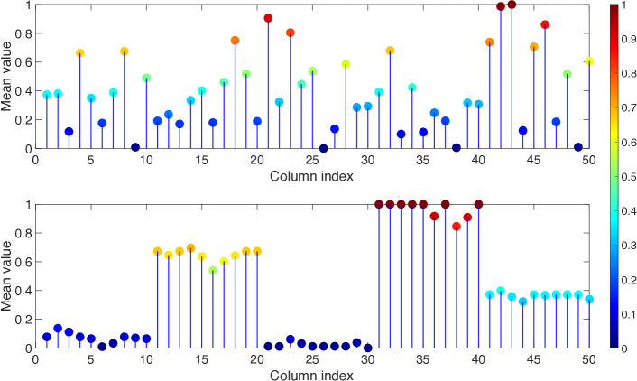
(a) The distribution of mean values of the columns in a frontal slice of $\mathcal{Z}$ (top) and $\mathcal{X}$ (bottom)

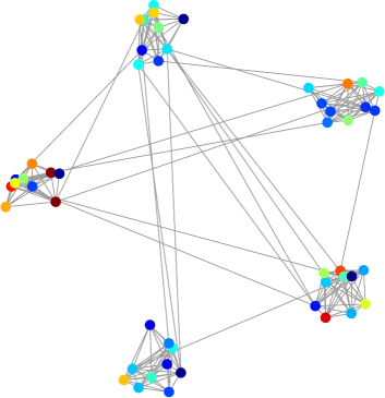
(b) The distribution of $\mathcal{Z}$ lies in the graph

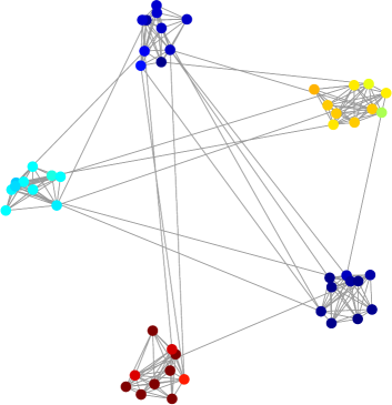
(c) The distribution of $\mathcal{X}$ lies in the graph

Figure 5: An illustration of the pairwise similarities of the entries in tensor $\mathcal{Z}$ and $\mathcal{X}$, and whether the similarities agree with the graph.

In the following experiments, we evaluate the recovery performance on the above tubal rank 5 tensor $\mathcal{X}\in\mathbb{R}^{50\times 50\times 64}$ with dynamic graphs $\mathcal{G}^{\mathcal{W}}$and $\mathcal{G}^{\mathcal{H}}$, where the degree of graph dynamism is controlled by length of time interval in $\{4,8,16,32,64\}$. To this end, we randomly sample a certain percentage of entries as the observation, where the sample ratio varies from $\{0.01,0.05,0.1,0.15,0.2,0.25,0.3,0.35,0.4,0.45,0.5\}$, and the rest entries are used as the test set on which we evaluate the recovery performance by the relative error:

$$\text{relative error (RE)}=\frac{\|\check{\mathcal{X}}_{test}-\mathcal{X}_{test}\|_{F}}{\|\mathcal{X}_{test}\|_{F}},$$

where $\check{\mathcal{X}}$ denotes the recovered tensor, and subscript $\mathcal{X}_{test}$ means the subset of the corresponding tensor on the test set.

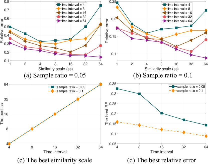
Figure 6: (a)(b) Recovery relative errors with respect to various similarity scales in our model to reconstruct the tensors with dynamic graphs, where the degree of dynamism is controlled by various time intervals, and sample ratio = 0.05, 0.1, respectively. (c)(d) The best similarity scales in our model and corresponding relative errors to recover the tensors with dynamic graphs with those time intervals.

7.1.3 Degree of Dynamism Versus Similarity Scale

In our model, similarity scale ($ss$) is employed to accommodate to different degrees of dynamics of the graphs, i.e., for relatively strong dynamics we should choose a smaller $ss$ to exploit the similarity structure in a more fine-grained manner. To verify the adaptability of $ss$ to different degrees of graph dynamism, we first generate random tensors and corresponding dynamic graphs with various time intervals, where the smaller time interval reflects the more severe dynamics. For each time interval, we evaluate the recovery performance of our model with various $ss$, and show the relative error curves with respect to $ss$ in Fig. 6 (a) and (b). Furthermore, in order to display the comprehensive results more conveniently, for each time interval we obtain the $ss$ achieving the minimum relative error, and show the curves of those best $ss$ and corresponding relative errors with respect to the time intervals in Fig. 6 (c) and (d), respectively. From Fig. 6 we can see that: (1) the time intervals and corresponding best $ss$ show an obvious positive correlation, which demonstrates that $ss$ can effectively cope with the different degrees of graph dynamism; (2) the corresponding relative error gradually decreases as the time interval increases, which is also in line with expectations for that dramatic changes in the graph obviously increase the difficulty of tensor recovery.

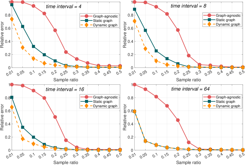
Figure 7: Performance of our model with (1) Graph-agnostic, (2) Static graph and (3) Dynamic graph model, for synthetic TC with graph information, where the sample ratios (the ratio of observed data) are $\{0.01,0.05,0.1,0.15,0.2,0.25,0.3,0.35,0.4,0.45,0.5\}$, and the dynamic graphs are generated with time intervals $4$ (top left), $8$ (top right), $16$ (bottom left), and $64$ (bottom right).

7.1.4 Graph Comparison

To evaluate the effectiveness of the dynamic graph based modeling and graph smoothness regularization in our model, we first compare our original model (named Dynamic graph model) with its two degenerated models: (1) a general TC model with no graph information (named Graph-agnostic model); (2) a TC model with static graphs (named Static graph model). The settings of those three models are as follows :
(1) Graph-agnostic: in our model setting the parameter of graph smoothness regularization as $\lambda_{\mathcal{G}}=0$. In this case graph information is not used and the model degenerates into a general TC model.
(2) Static graph: using the static graph of the first time period in $\mathcal{G}^{\mathcal{W}}$, $\mathcal{G}^{\mathcal{H}}$ as the graph information, and constructing static graph Laplacian tensors in our model. In this case the model degenerates into a TC model with static graphs.
(3) Dynamic graph: using the known dynamic graphs $\mathcal{G}^{\mathcal{W}}$, $\mathcal{G}^{\mathcal{H}}$ as the graph information, and employ the graph Laplacian tensors $\textbf{LAP}(\mathcal{G}^{\mathcal{W}})$ and $\textbf{LAP}(\mathcal{G}^{\mathcal{H}})$ in our model.

In Fig. 7 we plot the relative error curves of the three models with respect to various sample ratios and time interval of the graphs, which is the average results after repeating five times. From Fig. 7 we can see that:
(1) for all the four cases with various time interval, the two graph based models have obvious superiority to Graph-agnostic model, especially when the sample ratio is relatively small, which demonstrates the effectiveness of the proposed graph smoothness regularization in exploiting the pairwise similarities of the entries implicit in the graphs to improve the recovery performance.
(2) when time interval is 64, the graph information $\mathcal{G}^{\mathcal{W}}$, $\mathcal{G}^{\mathcal{H}}$ are essentially static graphs, and in this case model Dynamic graph and Static graph are exactly the same. While when time interval is 4, 8 or 16, Dynamic graph can achieve smaller relative errors than Static graph, and the advantage will be greater with smaller time interval. This is because Dynamic graph model takes the graph dynamism into consideration, while Static graph loses this information, which reflects the strength of the dynamic graph based modeling.

7.1.5 Parameters Sensitivity

We evaluate the parameters sensitivity of our model in the synthetic data, and show the results in Section 8 of the supplementary material, which demonstrates that our model is quite stable to parameters $\lambda_{\mathcal{G}}$ and $\lambda_{1}$, and thus parameters selection is not a tricky problem in our model.

7.1.6 Comparison with State-of-the-arts

We compare the recovery performance of our model with some state-of-the-art MC/TC methods, including GRMC, LRTC, TTC, TRNNM, TNN and GRTC. The four general TC methods LRTC, TTC, TRNNM and TNN just make use of the observations of the targeted tensor for recovery without considering graph information. GRMC is a MC method with graph information, and to deal with the tensor recovery case, we recover the frontal slices with graphs one by one. GRTC is a TC method with static graph, and we employ the graph of the first time period in $\mathcal{G}^{\mathcal{W}}$, $\mathcal{G}^{\mathcal{H}}$ as its static graph information. We do not compare with GNIMC here for that there is no feature matrix in the synthetic data. For our model the parameters are fixed as $\lambda_{\mathcal{G}}=\lambda_{1}=0.001$, and for the compared methods the model parameters are selected as the recommended or by five-fold cross validation. We repeat the experiments five times, and plot the averaged relative error curves with respect to sample ratios and various conversion probabilities in Fig. 8.

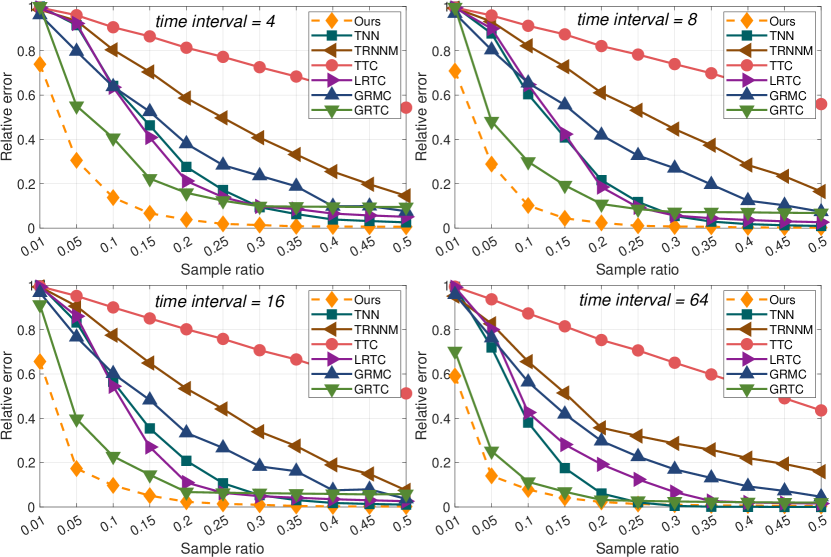
Figure 8: Performance of the compared methods for synthetic TC with graph information, where the sample ratios (the ratio of observed data) are from $0.01\sim 0.5$, and the dynamic graphs are generated with time intervals $4$ (top left), $8$ (top right), $16$ (bottom left), and $64$ (bottom right).

From Fig. 8, it can be seen that:
(1) for the four general TC methods, TRNNM, TTC performs poorly on all the various time interval cases. TNN, LRTC can achieve good recovery performance when sample ratios are relatively large, but will quickly deteriorates as the sampling ratio decreases. This is because those general methods only exploit tensor low rank property and thus are difficult to fully explore the inherent structure.
(2) as a MC method, GRMC has a natural deficiency in the tensor recovery problem. However, the performance of GRMC is comparable even better than those tensor based methods, giving the credit to its graph modeling approach.
(3) by utilizing the static graphs, GRTC achieves superior performance to those general TC ones, which demonstrates the validity of graph similarity information in assisting the tensor recovery. Meanwhile, the performance of GRTC significantly deteriorates as the time interval decreases, reflecting its deficiency in the face of graph dynamics.
(4) in the case time interval = 64, the graph information is actually static graph, and the recovery performance of our method is similar as GRTC and superior to others, while in the dynamic graph cases time interval = 4, 8, 16, our method performs significantly better than all the compared ones. Meanwhile, our method shows good adaptability to the graph dynamism. This is mainly due to the effective exploitation of dynamic graph information in our model.

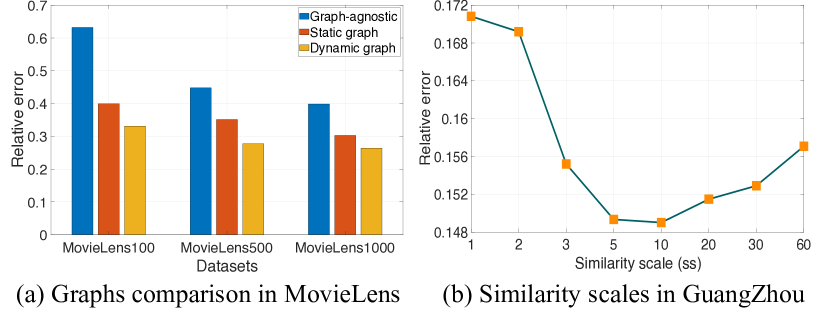
Figure 9: (a) Recovery relative errors of various graph models in MovieLens dataset; (b) Recovery relative errors with respect to similarity scales (ss) in GuangZhou dataset.

7.2 Collaborative Filtering

In this subsection we evaluate the proposed method on a real application of TC problem, collaborative filtering (CF)[75, 76], the de facto standard for analyzing users’ activities and building recommendation systems for items. A common strategy for CF is to construct $user\times item$ rating matrices or $user\times item\times context$ rating tensors, and then predict the missing ratings based on the partially observed ones using MC/TC approaches.

7.2.1 Dataset Introduction

We employ a well-known benchmark dataset MovieLens-1M  [77] which contains $1,000,000$ movie ratings from 6040 users on 3900 movies along with the user/movie features. In this dataset, each rating has a time stamp, and each user/movie has a 22/18 dimensional feature vector. Therefore, we can obtain a $6040\times 3900\times 6$ sparse tensor after time period splitting, and this tensor has feature matrices along its first and second mode. In order to decrease computational consumption, we randomly select $100,500,1000$ users and movies to construct three targeted tensors, and the details of the sub-datasets are presented in TABLE III.

TABLE III: sub-datasets of MovieLens-1M Used In the Experiments

Dataset	#Entries	#Mode1	#Mode2	Sparsity
MovieLens100	466	88	70	1.26%
MovieLens500	10966	500	411	0.89%
MovieLens1000	42205	999	875	0.82%

7.2.2 Graph Construction and Comparison

As the given data lacks graph information, we can address this limitation by constructing artificial user-wise and movie-wise similarity graphs. In a nutshell, we first generate new features of variables concatenating artificial and raw features, and then construct the static and dynamic graphs based on the feature distances, respectively. The specific construction processes are described in Section 9 of the supplementary material. In Fig. 9 (a) we compare the performance of various graph models, which demonstrates the effectiveness of the dynamic graph modeling.

7.2.3 Parameters Sensitivity

Due to that the total time periods are quite small ($T=6$), we just set similarity scale as $ss=6$ in this dataset. On this basis, we also evaluate the parameters sensitivity, including $\lambda_{\mathcal{G}}$, $\lambda_{1}$ and rank $r$, of our model in MovieLens100 and MovieLens500, and show the results in Section 10 of the supplementary material, highlighting the stability of our model to the parameters.

7.2.4 Feature Based Versus Graph Based Modeling

In our model we construct artificial pairwise similarity graphs using user/movie features, and improve the recovery performance by dynamic graph smoothness regularization. Actually, given additional user/movie features, a straightforward way is to recover a low-rank matrix from few observations while incorporating the features into completion model, which is usually called inductive MC problem. We then show that compared with directly incorporating features in the model, graph based modeling can be more robust to the feature noises. To this end, we add Gaussian noises with various noise levels into the user/movie features, and compare the recovery performance of our model with a representative inductive MC method GNIMC. In Fig. 10, we show the averaged relative errors and corresponding standard deviations of our model and GNIMC with respect to various feature noise levels. It can be seen that GNIMC is quite sensitive to the features noises, while our method shows good robustness.

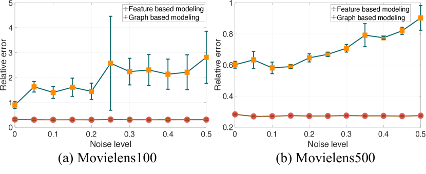
Figure 10: Recovery relative errors and corresponding standard deviations of our model and GNIMC with respect to various feature noise levels.

TABLE IV: Recovery Performances of the Tested Methods on the MovieLens Dataset.

Methods	MovieLens100		MovieLens500		MovieLens1000
	mean	std	mean	std	mean	std
GRMC	0.4156	0.0212	0.3593	0.0158	0.3642	0.0126
GNIMC	0.8669	0.0283	0.6501	0.0141	0.4686	0.0167
LRTC	0.6257	0.0291	0.3497	0.0157	0.3102	0.0117
TTC	0.4090	0.0240	0.3280	0.0149	0.3035	0.0116
TRNNM	0.7948	0.0245	0.6149	0.0146	0.6146	0.0119
TNN	0.5140	0.0283	0.3242	0.0155	0.3032	0.0121
GRTC	0.4996	0.0241	0.3286	0.0145	0.3008	0.0113
OURS	0.3094	0.0209	0.2755	0.0138	0.2647	0.0113

7.2.5 Comparison with State-of-the-arts

We evaluate the recovery performance of our model in comparison to the MC/TC methods mentioned earlier, using all three datasets. For each dataset, we randomly divide 80% of the known ratings as training data and use the remaining data as test data. For our model we just fixed the parameters $\lambda_{\mathcal{G}}=\lambda_{1}=0.001$, and select tubal rank by five-fold cross validation. For the compared methods the model parameters are selected as the recommended or by five-fold cross validation. We conduct the experiments five times and present the averaged relative errors and corresponding standard deviations in TABLE IV. The results demonstrate that our method consistently achieves the lowest relative errors and standard deviations across all three datasets, confirming its superiority.

7.3 Spatiotemporal Traffic Data Imputation

In the past few years, the rapid development of intelligent transportation systems has led to the collection and storage of vast amounts of urban spatiotemporal traffic data, which plays an important role in many traffic operation and management domains [58, 20]. In real-life situations, the collected traffic data often suffers from the problem of missing data due to the detector and communication malfunctions, leading to a strong demand for data imputation in traffic data applications. Usually, the spatiotemporal traffic data can be organized into a multi-dimensional array (such as the speed information in $road\ segment\times time\ of\ day\times day$ structure) with day-to-day recurrence and neighborhood similarity, and thus low-rank TC has proven a superior approach for traffic data imputation [19, 78]. Furthermore, the traffic states such as speeds and link volumes often presents obvious pairwise similarities on different time periods and road segments: for the former, there can form clusters between peak hours and off-peak hours; for the latter, similar road conditions tend to have similar traffic states. Thus the exploitation of pairwise similarities by graph smoothness is potentially helpful to the tensor recovery of spatiotemporal traffic data [19, 20].

7.3.1 Dataset Introduction

We evaluate the recovery performance of the proposed method on two spatiotemporal traffic datasets, GuangZhou and Portland . GuangZhou is a traffic speed data set collected in Guangzhou, China consisting of travel speed observations from 214 road segments in two months (61 days from August 1, 2016 to September 30, 2016) at 10-min interval (144 time intervals in a day). The GuangZhou data can be organized as a third-order tensor ($road\ segment\times time\ interval\times day$) with size $214\times 144\times 60$ after removing the observations in August 31. Portland collects the link volume from highways in Portland, USA containing 1156 loop detectors within one month at 15-minute interval, from which we construct a tensor ($loop\ detectors\times time\ interval\times day$) with size $80\times 96\times 15$ to decrease computational consumption.

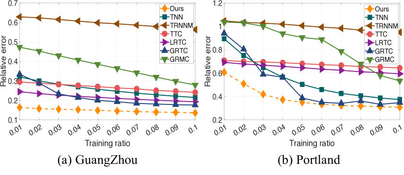
Figure 11: Recovery relative errors of the compared methods with respect to various sample ratios on (a) GuangZhou and (b) Portland.

7.3.2 Graph Construction and Comparison

Since there are no additional features available in the GuangZhou and Portland datasets, we can overcome this limitation by constructing artificial similarity graphs solely based on artificial features. We also showcase the corresponding graph construction and comparison in Section 11 of the supplementary material due to page limitations.

7.3.3 The Role of Similarity Scale

On the GuangZhou dataset with $T=60$, we can verify the adaptability of the model to graph dynamics, and plot the recovery relative error curve with respect to various similarity scales in Fig. 9 (b). It can be seen that the lowest error can be achieved in $ss=5,10$, which demonstrates that our model can accommodate to the graph dynamics through different similarity scales. As for Portland with quite small $T$, we just set $ss=T$.

7.3.4 Comparison with State-of-the-arts

We compare the recovery performance of all the methods on the two datasets, at various sample ratios, where the parameters setting are similar as in Section 7.2.5. The recovery relative errors with respect to the sample ratios are plotted in Fig. 11. It is evident that our method outperforms the other methods, demonstrating superior performance. Additionally, in Fig. 12 we showcase some visualization examples of the recovery performance. These examples highlight the high accuracy of our model in imputing plausible values from partially observed data.

8 Conclusion

Aiming at the dynamic nature of supplementary graphs in tensor related applications, in this work we systematically establish a new model, theoretical and algorithmic framework for the dynamic graph regularized tensor completion problem. In model, we establish a rigorous mathematical representation of the dynamic graph, based on which we derive a new tensor-oriented graph smoothness regularization. The new regularization can exploit the tensor‘s global pairwise similarity structure underlying in the dynamic graph. Incorporating the new regularization into transformed t-SVD, we build a new dynamic graph regularized TC model simultaneously exploiting the low-rank and pairwise similarity structure of tensors. In theory, we demonstrate that the proposed graph smoothness regularization is actually equivalent to a weighted tensor nuclear norm, where the weights implicitly characterize the graph information. Then, we build statistical consistency guarantees for our model. To the best of our knowledge, this should be the first theoretical guarantee among all related graph regularized tensor recovery studies, which fills a gap in the theoretical analysis of the tensor recovery with graph information. In algorithm, we develop a ADMM algorithm with convergence guarantees to solve the resulting model, and it is shown that the algorithm has lower computational complexity than the alternative ones. A series of experiments on synthetic and real-world data are carried out, demonstrating the superiority of our model over state-of-the-art TC methods, especially in scenarios with fewer accessible observations.

In this work we focus on the TC with graph information under uniformly sampling, and it would be of great interest to consider this problem under arbitrary sampling schemes in the future work. In addition, extending our results to higher-order tensors is also an interesting direction of future research.

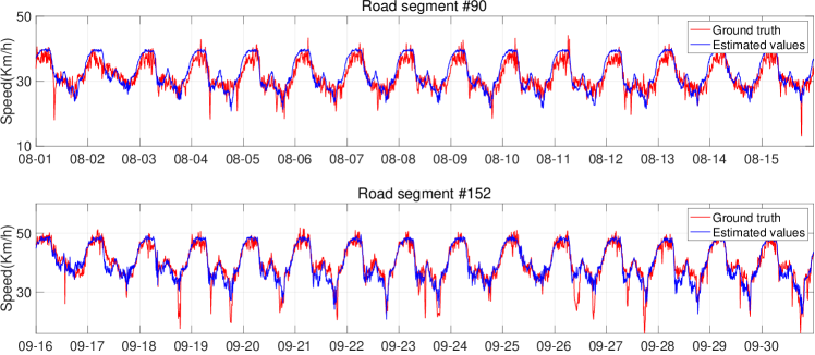
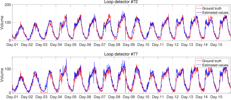
Figure 12: Visualization examples of imputation for GuangZhou (top two rows) and Portland (bottom two rows) with sample ratio $0.1$.

References

- [1] C. Diao, D. Zhang, W. Liang, K.-C. Li, Y. Hong, and J.-L. Gaudiot, “A novel spatial-temporal multi-scale alignment graph neural network security model for vehicles prediction,” IEEE Transactions on Intelligent Transportation Systems, vol. 24, no. 1, pp. 904–914, 2022.
- [2] B. B. Gupta, A. Gaurav, E. C. Marín, and W. Alhalabi, “Novel graph-based machine learning technique to secure smart vehicles in intelligent transportation systems,” IEEE Transactions on Intelligent Transportation Systems, 2022.
- [3] J. H. Giraldo, S. Javed, and T. Bouwmans, “Graph moving object segmentation,” IEEE Transactions on Pattern Analysis and Machine Intelligence, vol. 44, no. 5, pp. 2485–2503, 2020.
- [4] A. Mondal, J. H. Giraldo, T. Bouwmans, A. S. Chowdhury et al., “Moving object detection for event-based vision using graph spectral clustering,” in Proceedings of the IEEE/CVF International Conference on Computer Vision, 2021, pp. 876–884.
- [5] S. Javed, A. Mahmood, J. Dias, L. Seneviratne, and N. Werghi, “Hierarchical spatiotemporal graph regularized discriminative correlation filter for visual object tracking,” IEEE Transactions on Cybernetics, vol. 52, no. 11, pp. 12 259–12 274, 2021.
- [6] J. He, Z. Huang, N. Wang, and Z. Zhang, “Learnable graph matching: Incorporating graph partitioning with deep feature learning for multiple object tracking,” in Proceedings of the IEEE/CVF Conference on Computer Vision and Pattern Recognition, 2021, pp. 5299–5309.
- [7] S. Wu, F. Sun, W. Zhang, X. Xie, and B. Cui, “Graph neural networks in recommender systems: a survey,” ACM Computing Surveys, vol. 55, no. 5, pp. 1–37, 2022.
- [8] L. Wu, J. Li, P. Sun, R. Hong, Y. Ge, and M. Wang, “Diffnet++: A neural influence and interest diffusion network for social recommendation,” IEEE Transactions on Knowledge and Data Engineering, vol. 34, no. 10, pp. 4753–4766, 2020.
- [9] H.-C. Yi, Z.-H. You, D.-S. Huang, and C. K. Kwoh, “Graph representation learning in bioinformatics: trends, methods and applications,” Briefings in Bioinformatics, vol. 23, no. 1, p. bbab340, 2022.
- [10] W. Wu, W. Zhang, W. Hou, and X. Ma, “Multi-view clustering with graph learning for scrna-seq data,” IEEE/ACM Transactions on Computational Biology and Bioinformatics, 2023.
- [11] C. Jo and K. Lee, “Discrete-valued latent preference matrix estimation with graph side information,” in International Conference on Machine Learning. PMLR, 2021, pp. 5107–5117.
- [12] Q. Zhang, V. Y. Tan, and C. Suh, “Community detection and matrix completion with social and item similarity graphs,” IEEE Transactions on Signal Processing, vol. 69, pp. 917–931, 2021.
- [13] Y. Hu, L. Deng, H. Zheng, X. Feng, and Y. Chen, “Network latency estimation with graph-laplacian regularization tensor completion,” in GLOBECOM 2020-2020 IEEE Global Communications Conference. IEEE, 2020, pp. 1–6.
- [14] X. Chen, L.-G. Sun, and Y. Zhao, “Ncmcmda: mirna–disease association prediction through neighborhood constraint matrix completion,” Briefings in Bioinformatics, vol. 22, no. 1, pp. 485–496, 2021.
- [15] L. Li, Z. Gao, Y.-T. Wang, M.-W. Zhang, J.-C. Ni, C.-H. Zheng, and Y. Su, “Scmfmda: predicting microrna-disease associations based on similarity constrained matrix factorization,” PLoS Computational Biology, vol. 17, no. 7, p. e1009165, 2021.
- [16] F. Huang, X. Yue, Z. Xiong, Z. Yu, S. Liu, and W. Zhang, “Tensor decomposition with relational constraints for predicting multiple types of microrna-disease associations,” Briefings in Bioinformatics, vol. 22, no. 3, p. bbaa140, 2021.
- [17] D. Ouyang, R. Miao, J. Wang, X. Liu, S. Xie, N. Ai, Q. Dang, and Y. Liang, “Predicting multiple types of associations between mirnas and diseases based on graph regularized weighted tensor decomposition,” Frontiers in Bioengineering and Biotechnology, vol. 10, p. 911769, 2022.
- [18] J. Tang, X. Shu, Z. Li, Y.-G. Jiang, and Q. Tian, “Social anchor-unit graph regularized tensor completion for large-scale image retagging,” IEEE Transactions on Pattern Analysis and Machine Intelligence, vol. 41, no. 8, pp. 2027–2034, 2019.
- [19] L. Deng, X.-Y. Liu, H. Zheng, X. Feng, and Y. Chen, “Graph spectral regularized tensor completion for traffic data imputation,” IEEE Transactions on Intelligent Transportation Systems, vol. 23, no. 8, pp. 10 996–11 010, 2021.
- [20] T. Nie, G. Qin, Y. Wang, and J. Sun, “Correlating sparse sensing for large-scale traffic speed estimation: A laplacian-enhanced low-rank tensor kriging approach,” Transportation Research Part C: Emerging Technologies, vol. 152, p. 104190, 2023.
- [21] X. Zhang and M. K. Ng, “Low rank tensor completion with poisson observations,” IEEE Transactions on Pattern Analysis and Machine Intelligence, vol. 44, no. 8, pp. 4239–4251, 2021.
- [22] W. Qin, H. Wang, F. Zhang, J. Wang, X. Luo, and T. Huang, “Low-rank high-order tensor completion with applications in visual data,” IEEE Transactions on Image Processing, vol. 31, pp. 2433–2448, 2022.
- [23] J. D. Carroll and J.-J. Chang, “Analysis of individual differences in multidimensional scaling via an n-way generalization of “eckart-young” decomposition,” Psychometrika, vol. 35, no. 3, pp. 283–319, 1970.
- [24] L. R. Tucker, “Some mathematical notes on three-mode factor analysis,” Psychometrika, vol. 31, no. 3, pp. 279–311, 1966.
- [25] T. G. Kolda and B. W. Bader, “Tensor decompositions and applications,” SIAM Review, vol. 51, no. 3, pp. 455–500, 2009.
- [26] I. V. Oseledets, “Tensor-train decomposition,” SIAM Journal on Scientific Computing, vol. 33, no. 5, pp. 2295–2317, 2011.
- [27] Q. Zhao, G. Zhou, S. Xie, L. Zhang, and A. Cichocki, “Tensor ring decomposition,” arXiv preprint arXiv:1606.05535, 2016.
- [28] M. E. Kilmer and C. D. Martin, “Factorization strategies for third-order tensors,” Linear Algebra and its Applications, vol. 435, no. 3, pp. 641–658, 2011.
- [29] E. Kernfeld, M. Kilmer, and S. Aeron, “Tensor–tensor products with invertible linear transforms,” Linear Algebra and its Applications, vol. 485, pp. 545–570, 2015.
- [30] M. E. Kilmer, K. Braman, N. Hao, and R. C. Hoover, “Third-order tensors as operators on matrices: A theoretical and computational framework with applications in imaging,” SIAM Journal on Matrix Analysis and Applications, vol. 34, no. 1, pp. 148–172, 2013.
- [31] T.-X. Jiang, M. K. Ng, X.-L. Zhao, and T.-Z. Huang, “Framelet representation of tensor nuclear norm for third-order tensor completion,” IEEE Transactions on Image Processing, vol. 29, pp. 7233–7244, 2020.
- [32] Q. Gao, P. Zhang, W. Xia, D. Xie, X. Gao, and D. Tao, “Enhanced tensor rpca and its application,” IEEE Transactions on Pattern Analysis and Machine Intelligence, vol. 43, no. 6, pp. 2133–2140, 2020.
- [33] C. Lu, J. Feng, Y. Chen, W. Liu, Z. Lin, and S. Yan, “Tensor robust principal component analysis with a new tensor nuclear norm,” IEEE Transactions on Pattern Analysis and Machine Intelligence, vol. 42, no. 4, pp. 925–938, 2019.
- [34] F. Zhang, J. Wang, W. Wang, and C. Xu, “Low-tubal-rank plus sparse tensor recovery with prior subspace information,” IEEE Transactions on Pattern Analysis and Machine Intelligence, vol. 43, no. 10, pp. 3492–3507, 2020.
- [35] L. Chen, X. Jiang, X. Liu, and Z. Zhou, “Robust low-rank tensor recovery via nonconvex singular value minimization,” IEEE Transactions on Image Processing, vol. 29, pp. 9044–9059, 2020.
- [36] V. Kalofolias, X. Bresson, M. Bronstein, and P. Vandergheynst, “Matrix completion on graphs,” arXiv preprint arXiv:1408.1717, 2014.
- [37] N. Rao, H.-F. Yu, P. K. Ravikumar, and I. S. Dhillon, “Collaborative filtering with graph information: Consistency and scalable methods,” Advances in Neural Information Processing Systems, vol. 28, 2015.
- [38] A. Elmahdy, J. Ahn, C. Suh, and S. Mohajer, “Matrix completion with hierarchical graph side information,” Advances in Neural Information Processing Systems, vol. 33, pp. 9061–9074, 2020.
- [39] S. Dong, P.-A. Absil, and K. Gallivan, “Riemannian gradient descent methods for graph-regularized matrix completion,” Linear Algebra and its Applications, vol. 623, pp. 193–235, 2021.
- [40] M. Ashraphijuo and X. Wang, “Fundamental conditions for low-cp-rank tensor completion,” The Journal of Machine Learning Research, vol. 18, no. 1, pp. 2116–2145, 2017.
- [41] N. Ghadermarzy, Y. Plan, and Ö. Yilmaz, “Near-optimal sample complexity for convex tensor completion,” Information and Inference: A Journal of the IMA, vol. 8, no. 3, pp. 577–619, 2019.
- [42] Q. Zhao, L. Zhang, and A. Cichocki, “Bayesian cp factorization of incomplete tensors with automatic rank determination,” IEEE Transactions on Pattern Analysis and Machine Intelligence, vol. 37, no. 9, pp. 1751–1763, 2015.
- [43] J. Liu, P. Musialski, P. Wonka, and J. Ye, “Tensor completion for estimating missing values in visual data,” IEEE Transactions on Pattern Analysis and Machine Intelligence, vol. 35, no. 1, pp. 208–220, 2012.
- [44] B. Romera-Paredes and M. Pontil, “A new convex relaxation for tensor completion,” Advances in Neural Information Processing Systems, vol. 26, 2013.
- [45] C. Mu, B. Huang, J. Wright, and D. Goldfarb, “Square deal: Lower bounds and improved relaxations for tensor recovery,” in International Conference on Machine Learning, 2014, pp. 73–81.
- [46] M. Ashraphijuo, V. Aggarwal, and X. Wang, “Deterministic and probabilistic conditions for finite completability of low-tucker-rank tensor,” IEEE Transactions on Information Theory, vol. 65, no. 9, pp. 5380–5400, 2019.
- [47] D. Xia and M. Yuan, “On polynomial time methods for exact low-rank tensor completion,” Foundations of Computational Mathematics, vol. 19, no. 6, pp. 1265–1313, 2019.
- [48] O. Semerci, N. Hao, M. E. Kilmer, and E. L. Miller, “Tensor-based formulation and nuclear norm regularization for multienergy computed tomography,” IEEE Transactions on Image Processing, vol. 23, no. 4, pp. 1678–1693, 2014.
- [49] Z. Zhang, G. Ely, S. Aeron, N. Hao, and M. Kilmer, “Novel methods for multilinear data completion and de-noising based on tensor-svd,” in Proceedings of the IEEE Conference on Computer Vision and Pattern Recognition, 2014, pp. 3842–3849.
- [50] Z. Zhang and S. Aeron, “Exact tensor completion using t-svd,” IEEE Transactions on Signal Processing, vol. 65, no. 6, pp. 1511–1526, 2016.
- [51] P. Zhou, C. Lu, Z. Lin, and C. Zhang, “Tensor factorization for low-rank tensor completion,” IEEE Transactions on Image Processing, vol. 27, no. 3, pp. 1152–1163, 2017.
- [52] C. Lu, X. Peng, and Y. Wei, “Low-rank tensor completion with a new tensor nuclear norm induced by invertible linear transforms,” in Proceedings of the IEEE/CVF Conference on Computer Vision and Pattern Recognition, 2019, pp. 5996–6004.
- [53] J. Hou, F. Zhang, H. Qiu, J. Wang, Y. Wang, and D. Meng, “Robust low-tubal-rank tensor recovery from binary measurements,” IEEE Transactions on Pattern Analysis and Machine Intelligence, vol. 44, no. 8, pp. 4355–4373, 2021.
- [54] A. Wang, Z. Jin, and G. Tang, “Robust tensor decomposition via t-svd: Near-optimal statistical guarantee and scalable algorithms,” Signal Processing, vol. 167, p. 107319, 2020.
- [55] J. A. Bengua, H. N. Phien, H. D. Tuan, and M. N. Do, “Efficient tensor completion for color image and video recovery: Low-rank tensor train,” IEEE Transactions on Image Processing, vol. 26, no. 5, pp. 2466–2479, 2017.
- [56] W. Wang, V. Aggarwal, and S. Aeron, “Efficient low rank tensor ring completion,” in Proceedings of the IEEE International Conference on Computer Vision, 2017, pp. 5697–5705.
- [57] T. Zhou, H. Shan, A. Banerjee, and G. Sapiro, “Kernelized probabilistic matrix factorization: Exploiting graphs and side information,” in Proceedings of the 2012 SIAM International Conference on Data Mining. SIAM, 2012, pp. 403–414.
- [58] J.-M. Yang, Z.-R. Peng, and L. Lin, “Real-time spatiotemporal prediction and imputation of traffic status based on lstm and graph laplacian regularized matrix factorization,” Transportation Research Part C: Emerging Technologies, vol. 129, p. 103228, 2021.
- [59] Y. Guan, S. Dong, P.-A. Absil, and F. Glineur, “Alternating minimization algorithms for graph regularized tensor completion,” arXiv preprint arXiv:2008.12876, 2020.
- [60] Y. Xu, R. Hao, W. Yin, and Z. Su, “Parallel matrix factorization for low-rank tensor completion,” arXiv preprint arXiv:1312.1254, 2013.
- [61] H. Kasai and B. Mishra, “Low-rank tensor completion: a riemannian manifold preconditioning approach,” in International Conference on Machine Learning. PMLR, 2016, pp. 1012–1021.
- [62] X.-Y. Liu, S. Aeron, V. Aggarwal, and X. Wang, “Low-tubal-rank tensor completion using alternating minimization,” IEEE Transactions on Information Theory, vol. 66, no. 3, pp. 1714–1737, 2019.
- [63] A. Wang, Z. Lai, and Z. Jin, “Noisy low-tubal-rank tensor completion,” Neurocomputing, vol. 330, pp. 267–279, 2019.
- [64] A. Wang and Z. Jin, “Near-optimal noisy low-tubal-rank tensor completion via singular tube thresholding,” in 2017 IEEE International Conference on Data Mining Workshops (ICDMW). IEEE, 2017, pp. 553–560.
- [65] S. Negahban and M. J. Wainwright, “Restricted strong convexity and weighted matrix completion: Optimal bounds with noise,” The Journal of Machine Learning Research, vol. 13, no. 1, pp. 1665–1697, 2012.
- [66] O. KLOPP, “Noisy low-rank matrix completion with general sampling distribution,” Bernoulli, pp. 282–303, 2014.
- [67] A. Tsybakov, V. Koltchinskii, and K. Lounici, “Nuclear-norm penalization and optimal rates for noisy low-rank matrix completion,” Annals of Statistics, vol. 39, no. 5, pp. 2302–2329, 2011.
- [68] P. Zilber and B. Nadler, “Inductive matrix completion: No bad local minima and a fast algorithm,” in International Conference on Machine Learning. PMLR, 2022, pp. 27 671–27 692.
- [69] C. Chen, Z.-B. Wu, Z.-T. Chen, Z.-B. Zheng, and X.-J. Zhang, “Auto-weighted robust low-rank tensor completion via tensor-train,” Information Sciences, vol. 567, pp. 100–115, 2021.
- [70] H. Huang, Y. Liu, J. Liu, and C. Zhu, “Provable tensor ring completion,” Signal Processing, vol. 171, p. 107486, 2020.
- [71] M. Girvan and M. E. Newman, “Community structure in social and biological networks,” Proceedings of the National Academy of Sciences, vol. 99, no. 12, pp. 7821–7826, 2002.
- [72] N. Perraudin, J. Paratte, D. Shuman, L. Martin, V. Kalofolias, P. Vandergheynst, and D. K. Hammond, “Gspbox: A toolbox for signal processing on graphs,” arXiv preprint arXiv:1408.5781, 2014.
- [73] D. Shuman, S. Narang, P. Frossard, A. Ortega, and P. Vanderghenyst, “The emmerging field of signal processing on graphs,” IEEE Signal Proc. Magazine, 2013.
- [74] D. I. Shuman, B. Ricaud, and P. Vandergheynst, “Vertex-frequency analysis on graphs,” Applied and Computational Harmonic Analysis, vol. 40, no. 2, pp. 260–291, 2016.
- [75] B. Yang, Y. Lei, J. Liu, and W. Li, “Social collaborative filtering by trust,” IEEE Transactions on Pattern Analysis and Machine Intelligence, vol. 39, no. 8, pp. 1633–1647, 2016.
- [76] W. Yu and Z. Qin, “Graph convolutional network for recommendation with low-pass collaborative filters,” in International Conference on Machine Learning. PMLR, 2020, pp. 10 936–10 945.
- [77] F. M. Harper and J. A. Konstan, “The movielens datasets: History and context,” Acm Transactions on Interactive Intelligent Systems (TIIS), vol. 5, no. 4, pp. 1–19, 2015.
- [78] T. Nie, G. Qin, and J. Sun, “Truncated tensor schatten p-norm based approach for spatiotemporal traffic data imputation with complicated missing patterns,” Transportation Research Part C: Emerging Technologies, vol. 141, p. 103737, 2022.