Unidirectional Superconductivity and Diode Effect Induced by Dissipation
Akito Daido
Department of Physics, Graduate School of Science, Kyoto University, Kyoto 606-8502, Japan
daido@scphys.kyoto-u.ac.jp
Youichi Yanase
Department of Physics, Graduate School of Science, Kyoto University, Kyoto 606-8502, Japan
Abstract
A general principle of condensed matter physics prohibits the electric current in equilibrium.
This prevents a zero-resistance state realized solely under a finite electric current, namely the unidirectional superconductivity.
In this Letter, we propose a setup to realize the unidirectional superconductivity as a nonequilibrium steady state.
We focus on the in-plane transport of atomically thin bilayer superconductors lacking the in-plane inversion symmetry and introduce dissipation by applying the out-of-plane electric field and current.
By analyzing the time-dependent Ginzburg-Landau equations, we show that locally stable steady-state solutions appear only under the in-plane supercurrent when the out-of-plane electric field exceeds a threshold value.
Our system also realizes the dissipation-induced superconducting diode effect up to 100 % percent 100 100\%
Introduction . —
Current-related phenomena in superconductors are among the most important topics in condensed matter physics.
The recent experiment of the superconducting diode effect (SDE) in Nb/V/Ta superlattices [1 ] has brought about a number of theoretical and experimental studies with particular emphasis on the potential role of the bulk inversion symmetry breaking [2 , 3 , 4 , 5 , 6 , 7 , 8 , 9 , 10 , 11 , 12 ] .
SDE refers to the situation
where the critical currents for the positive and negative directions, namely j c ± subscript 𝑗 limit-from c plus-or-minus j_{\rm c\pm} 1 [13 , 14 , 15 , 16 , 17 , 18 , 19 ] but also the intrinsic mechanism by finite-momentum Cooper pairs can cause SDE [8 , 9 , 10 , 11 , 12 , 7 ] , shedding light on the potential application of SDE for probing exotic superconducting states.
Nonreciprocal resistivity during the superconducting transition is also attracting much attention [20 , 21 , 22 , 23 , 24 , 25 , 26 , 27 , 28 ] .
Further study of the current-related phenomena in superconductors is indispensable both from fundamental-physics and engineering viewpoints.
Among various experiments of SDE, a notable result has been reported for the twisted trilayer graphene [5 , 7 ] . In this system,
either j c + subscript 𝑗 limit-from c j_{\rm c+} j c − subscript 𝑗 limit-from c j_{\rm c-} 1 [29 , 30 , 31 ] .
Specifically, in the mean-field approximation, the free energy F 𝐹 F j 𝑗 j q 𝑞 q j = 2 ∂ F / ∂ q 𝑗 2 𝐹 𝑞 j=2\partial F/\partial q [32 ] .
This ensures j = 0 𝑗 0 j=0 j > 0 𝑗 0 j>0 j < 0 𝑗 0 j<0 j c ± subscript 𝑗 limit-from c plus-or-minus j_{\rm c\pm}
We must circumvent the above discussion to achieve a zero-resistance state only under a finite electric current, namely, the unidirectional superconductivity (USC).
One way is to assume
a strong dependence of system parameters on the electric current.
Actually, it is pointed out that USC in twisted trilayer graphene might be understood by destabilization of the coexisting symmetry-breaking order detrimental to superconductivity [7 ] .
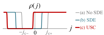
Figure 1:
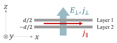
Schematic of current-resistivity relation ρ ( j ) 𝜌 𝑗 \rho(j) Figure 2: Schematic figure of the system.
We consider a wire or thin film uniform in the y 𝑦 y E ⟂ subscript 𝐸 perpendicular-to E_{\perp} j ⟂ subscript 𝑗 perpendicular-to j_{\perp} z 𝑧 z j ∥ subscript 𝑗 parallel-to j_{\parallel} x 𝑥 x
Such a scenario, however, relies on nontrivial assumptions of the underlying exotic order and is difficult to quantify.
This stands in the way of predicting new USC candidates.
In this Letter, we propose another direction to achieve USC, i.e., driving the system out of equilibrium.
As a source of dissipation, we focus on the d.c. electric field and current, which should be applied perpendicular to the system to study the in-plane supercurrent [Fig. 2 [33 , 34 ] , while vanishes in the bulk.
Thus,
superconducting wires and films thinner than the coherence length would provide the platform for USC.
In the following, we focus on atomically-thin bilayer superconductors as a minimal setup.
From the symmetry viewpoint,
in-plane inversion and time-reversal symmetries
must be broken to achieve SDE [8 , 9 , 10 , 11 , 12 ] and therefore USC.
We require the crystal structure to satisfy the former
while the latter is accomplished by dissipation.
We demonstrate that such a bilayer superconductor actually realizes USC as a nonequilibrium steady state, based on the time-dependent Ginzburg-Landau (TDGL) equation.
Our result uncovers a scheme to realize ideal superconducting diodes by purely electric means and provides an interesting example of the nonreciprocal phase transition [35 ] in nonequilibrium quantum materials.
Bilayer superconductor in equilibrium. —
Let us first discuss the equilibrium properties in the absence of the perpendicular electric field [Fig. 2
F [ 𝝍 ] = N 0 ∫ 𝑑 x 𝝍 † ( x ) α ^ ( ∇ / i ) 𝝍 ( x ) + β 0 2 [ 𝝍 † ( x ) 𝝍 ( x ) ] 2 , 𝐹 delimited-[] 𝝍 subscript 𝑁 0 differential-d 𝑥 superscript 𝝍 † 𝑥 ^ 𝛼 ∇ 𝑖 𝝍 𝑥 subscript 𝛽 0 2 superscript delimited-[] superscript 𝝍 † 𝑥 𝝍 𝑥 2 \!\!\!\!F[\bm{\psi}]=N_{0}\!\!\int\!dx\,\bm{\psi}^{\dagger}(x)\hat{\alpha}(\nabla/i)\bm{\psi}(x)+\frac{\beta_{0}}{2}[\bm{\psi}^{\dagger}(x)\bm{\psi}(x)]^{2}, (1)
where each component of 𝝍 ( x ) = ( ψ 1 ( x ) , ψ 2 ( x ) ) T 𝝍 𝑥 superscript subscript 𝜓 1 𝑥 subscript 𝜓 2 𝑥 𝑇 \bm{\psi}(x)=\bigl{(}\psi_{1}(x),\psi_{2}(x)\bigr{)}^{T} z = ± d / 2 𝑧 plus-or-minus 𝑑 2 z=\pm d/2 N 0 subscript 𝑁 0 N_{0} β 0 subscript 𝛽 0 \beta_{0} α ^ ( ∇ / i ) = α 0 ( ∇ / i ) + 𝜶 ( ∇ / i ) ⋅ 𝝈 ^ 𝛼 ∇ 𝑖 subscript 𝛼 0 ∇ 𝑖 ⋅ 𝜶 ∇ 𝑖 𝝈 \hat{\alpha}(\nabla/i)=\alpha_{0}(\nabla/i)+\bm{\alpha}(\nabla/i)\cdot\bm{\sigma} σ i subscript 𝜎 𝑖 \sigma_{i}
It is convenient to introduce the plane-wave basis, replacing
∇ / i ∇ 𝑖 {\nabla}/i q 𝑞 q α ^ ∗ ( q ) = α ^ ( − q ) superscript ^ 𝛼 𝑞 ^ 𝛼 𝑞 \hat{\alpha}^{*}(q)=\hat{\alpha}(-q) α 0 ( q ) subscript 𝛼 0 𝑞 \alpha_{0}(q) α x ( q ) subscript 𝛼 𝑥 𝑞 \alpha_{x}(q) α z ( q ) subscript 𝛼 𝑧 𝑞 \alpha_{z}(q) q 𝑞 q α y ( q ) subscript 𝛼 𝑦 𝑞 \alpha_{y}(q) α 0 ( q ) = a 0 + a 0 ′′ q 2 , α x ( q ) = a x , α y ( q ) = a y ′ q , formulae-sequence subscript 𝛼 0 𝑞 subscript 𝑎 0 superscript subscript 𝑎 0 ′′ superscript 𝑞 2 formulae-sequence subscript 𝛼 𝑥 𝑞 subscript 𝑎 𝑥 subscript 𝛼 𝑦 𝑞 superscript subscript 𝑎 𝑦 ′ 𝑞 \alpha_{0}(q)=a_{0}+a_{0}^{\prime\prime}q^{2},\alpha_{x}(q)=a_{x},\alpha_{y}(q)=a_{y}^{\prime}q, 1 α z ( q ) = 0 subscript 𝛼 𝑧 𝑞 0 \alpha_{z}(q)=0 σ x α ^ ( q ) σ x = α ^ ( − q ) subscript 𝜎 𝑥 ^ 𝛼 𝑞 subscript 𝜎 𝑥 ^ 𝛼 𝑞 \sigma_{x}\hat{\alpha}(q)\sigma_{x}=\hat{\alpha}(-q) a y ′ = ∂ q α y ( q ) | q → 0 superscript subscript 𝑎 𝑦 ′ evaluated-at subscript 𝑞 subscript 𝛼 𝑦 𝑞 → 𝑞 0 a_{y}^{\prime}=\partial_{q}\alpha_{y}(q)|_{q\to 0} x 𝑥 x C 2 h subscript 𝐶 2 ℎ C_{2h} y 𝑦 y [36 ] .
We also introduce α ρ ( q ) subscript 𝛼 𝜌 𝑞 \alpha_{\rho}(q) α θ ( q ) subscript 𝛼 𝜃 𝑞 \alpha_{\theta}(q) ( α x ( q ) , α y ( q ) ) = α ρ ( q ) ( cos α θ ( q ) , sin α θ ( q ) ) subscript 𝛼 𝑥 𝑞 subscript 𝛼 𝑦 𝑞 subscript 𝛼 𝜌 𝑞 subscript 𝛼 𝜃 𝑞 subscript 𝛼 𝜃 𝑞 (\alpha_{x}(q),\alpha_{y}(q))=\alpha_{\rho}(q)(\cos\alpha_{\theta}(q),\sin\alpha_{\theta}(q))
The system undergoes a superconducting transition when the minimum eigenvalue of α ^ ( ∇ / i ) ^ 𝛼 ∇ 𝑖 \hat{\alpha}(\nabla/i) T 𝑇 T q 𝑞 q α ^ ( q ) ^ 𝛼 𝑞 \hat{\alpha}(q) α ± ( q ) = α 0 ( q ) ± α ρ ( q ) subscript 𝛼 plus-or-minus 𝑞 plus-or-minus subscript 𝛼 0 𝑞 subscript 𝛼 𝜌 𝑞 \alpha_{\pm}(q)=\alpha_{0}(q)\pm\alpha_{\rho}(q) α − ( q ) ≃ ϵ + ξ 0 2 q 2 + O ( q 4 ) similar-to-or-equals subscript 𝛼 𝑞 italic-ϵ superscript subscript 𝜉 0 2 superscript 𝑞 2 𝑂 superscript 𝑞 4 \alpha_{-}(q)\simeq\epsilon+\xi_{0}^{2}q^{2}+O(q^{4}) q = 0 𝑞 0 q=0 ξ 0 2 ≡ a 0 ′′ − a y ′ 2 / 2 | a x | superscript subscript 𝜉 0 2 superscript subscript 𝑎 0 ′′ superscript subscript 𝑎 𝑦 ′ 2
2 subscript 𝑎 𝑥 \xi_{0}^{2}\equiv a_{0}^{\prime\prime}-a_{y}^{\prime 2}/2|a_{x}| T c0 subscript 𝑇 c0 {T_{\rm c0}} ϵ ≡ ( T − T c0 ) / T c0 = a 0 − | a x | italic-ϵ 𝑇 subscript 𝑇 c0 subscript 𝑇 c0 subscript 𝑎 0 subscript 𝑎 𝑥 \epsilon\equiv(T-{T_{\rm c0}})/{T_{\rm c0}}=a_{0}-|a_{x}|
ψ ^ eq ( q ) ≃ 1 2 e − i 2 [ α θ ( 0 ) + a y ′ a x q ] σ z ( 1 − 1 ) . similar-to-or-equals subscript ^ 𝜓 eq 𝑞 1 2 superscript 𝑒 𝑖 2 delimited-[] subscript 𝛼 𝜃 0 superscript subscript 𝑎 𝑦 ′ subscript 𝑎 𝑥 𝑞 subscript 𝜎 𝑧 matrix 1 1 \hat{\psi}_{\rm eq}(q)\simeq\frac{1}{2}e^{-\frac{i}{2}\left[\alpha_{\theta}(0)+\frac{a_{y}^{\prime}}{a_{x}}q\right]\sigma_{z}}\begin{pmatrix}1\\
-1\end{pmatrix}. (2)
The Bardeen-Cooper-Schrieffer state ψ ^ eq ( 0 ) ∝ ( 1 , 1 ) T proportional-to subscript ^ 𝜓 eq 0 superscript 1 1 𝑇 \hat{\psi}_{\rm eq}({0})\propto(1,1)^{T} [37 , 38 ] ψ ^ eq ( 0 ) ∝ ( 1 , − 1 ) T proportional-to subscript ^ 𝜓 eq 0 superscript 1 1 𝑇 \hat{\psi}_{\rm eq}(0)\propto(1,-1)^{T} a x subscript 𝑎 𝑥 a_{x} q ≠ 0 𝑞 0 q\neq 0
The amplitude of the superconducting order parameter becomes finite for a negative reduced temperature ϵ < 0 italic-ϵ 0 \epsilon<0 𝝍 ( x ) 𝝍 𝑥 \bm{\psi}({x})
δ F δ 𝝍 † ( x ) = N 0 { α ^ ( ∇ / i ) + β 0 [ 𝝍 † ( x ) 𝝍 ( x ) ] } 𝝍 ( x ) = 0 . 𝛿 𝐹 𝛿 superscript 𝝍 † 𝑥 subscript 𝑁 0 ^ 𝛼 ∇ 𝑖 subscript 𝛽 0 delimited-[] superscript 𝝍 † 𝑥 𝝍 𝑥 𝝍 𝑥 0 \frac{\delta F}{\delta\bm{\psi}^{\dagger}(x)}=N_{0}\Bigl{\{}\hat{\alpha}(\nabla/i)+\beta_{0}[\bm{\psi}^{\dagger}(x)\bm{\psi}(x)]\Bigr{\}}\bm{\psi}(x)=0. (3)
This can be easily solved for the plain-wave ansatz.
By assuming 𝝍 ( x ) = e i q x R ( q ) ψ ^ ( q ) 𝝍 𝑥 superscript 𝑒 𝑖 𝑞 𝑥 𝑅 𝑞 ^ 𝜓 𝑞 \bm{\psi}({x})=e^{iqx}R(q)\hat{\psi}(q) R ( q ) ≥ 0 𝑅 𝑞 0 R(q)\geq 0 | ψ ^ ( q ) | = 1 ^ 𝜓 𝑞 1 |\hat{\psi}(q)|=1 ψ ^ ( q ) ^ 𝜓 𝑞 \hat{\psi}(q) α ^ ( q ) ^ 𝛼 𝑞 \hat{\alpha}(q) ψ ^ eq ( q ) subscript ^ 𝜓 eq 𝑞 \hat{\psi}_{\rm eq}(q) R eq ( q ) 2 = ( − ϵ − ξ 0 2 q 2 ) / β 0 subscript 𝑅 eq superscript 𝑞 2 italic-ϵ superscript subscript 𝜉 0 2 superscript 𝑞 2 subscript 𝛽 0 R_{\rm eq}(q)^{2}=(-\epsilon-\xi_{0}^{2}q^{2})/\beta_{0} q 𝑞 q
The supercurrent through the system is obtained by [36 ]
j ∥ ( q ) = 2 N 0 R 2 ( q ) ψ ^ † ( q ) ∂ q α ^ ( q ) ψ ^ ( q ) , subscript 𝑗 parallel-to 𝑞 2 subscript 𝑁 0 superscript 𝑅 2 𝑞 superscript ^ 𝜓 † 𝑞 subscript 𝑞 ^ 𝛼 𝑞 ^ 𝜓 𝑞 j_{\parallel}(q)=2N_{0}R^{2}(q)\hat{\psi}^{\dagger}(q)\partial_{q}\hat{\alpha}(q)\hat{\psi}(q), (4)
for any plain-wave order parameter.
We obtain
j eq ( q ) ≃ 4 N 0 ξ 0 2 β 0 q ( | ϵ | − ξ 0 2 q 2 ) , similar-to-or-equals subscript 𝑗 eq 𝑞 4 subscript 𝑁 0 superscript subscript 𝜉 0 2 subscript 𝛽 0 𝑞 italic-ϵ superscript subscript 𝜉 0 2 superscript 𝑞 2 j_{\rm eq}(q)\simeq\frac{4N_{0}\xi_{0}^{2}}{\beta_{0}}\,q\,(|\epsilon|-\xi_{0}^{2}q^{2}), (5)
for the equilibrium solution.
This is the conventional current-momentum relation [32 ] .
The maximum j c + subscript 𝑗 limit-from c {j_{\rm c+}} − j c − subscript 𝑗 limit-from c -{j_{\rm c-}} j eq ( q ) subscript 𝑗 eq 𝑞 {j_{\rm eq}}(q) j c + = j c − subscript 𝑗 limit-from c subscript 𝑗 limit-from c {j_{\rm c+}}={j_{\rm c-}}
Nonequilibrium steady states. —
Next, we discuss the nonequilibrium properties of the system.
The nonequilibrium dynamics of the order parameter can be phenomenologically understood by the TDGL equation
Γ ∂ t 𝝍 ( x , t ) = − δ F δ 𝝍 † ( x , t ) , Γ subscript 𝑡 𝝍 𝑥 𝑡 𝛿 𝐹 𝛿 superscript 𝝍 † 𝑥 𝑡 \Gamma\partial_{t}\bm{\psi}(x,t)=-\left.\frac{\delta F}{\delta\bm{\psi}^{\dagger}(x,t)}\right., (6)
where Γ > 0 Γ 0 \Gamma>0 ∂ t ≡ ∂ / ∂ t subscript 𝑡 𝑡 \partial_{t}\equiv\partial/\partial t 3 [33 ] ,
the simplified description offered by the TDGL formalism is useful to qualitatively understand and predict physical phenomena.
The effect of the electromagnetic field can be incorporated into Eq. (6 [36 ] .
In particular, the electric field can be introduced by ∂ t → ∂ t + 2 i ϕ → subscript 𝑡 subscript 𝑡 2 𝑖 italic-ϕ \partial_{t}\to\partial_{t}+2i\phi ϕ italic-ϕ \phi E ∥ subscript 𝐸 parallel-to E_{\parallel} ϕ = − E ∥ x italic-ϕ subscript 𝐸 parallel-to 𝑥 \phi=-E_{\parallel}x [39 , 40 , 34 , 33 ] , we focus on the d.c. electric field perpendicular to the system by ϕ = − E ⟂ d σ z / 2 italic-ϕ subscript 𝐸 perpendicular-to 𝑑 subscript 𝜎 𝑧 2 \phi=-E_{\perp}d\sigma_{z}/2 d 𝑑 d E ⟂ subscript 𝐸 perpendicular-to E_{\perp} 2 [33 ] .
Thus, assuming the plain-wave ansatz 𝝍 ( x , t ) = e i q x 𝝍 ( q , t ) 𝝍 𝑥 𝑡 superscript 𝑒 𝑖 𝑞 𝑥 𝝍 𝑞 𝑡 \bm{\psi}(x,t)=e^{iqx}\bm{\psi}(q,t) [36 ]
[ ∂ t + i Φ ] 𝝍 ( q , t ) = − [ α ^ ( q ) + β 0 | 𝝍 ( q , t ) | 2 ] 𝝍 ( q , t ) , delimited-[] subscript 𝑡 𝑖 Φ 𝝍 𝑞 𝑡 delimited-[] ^ 𝛼 𝑞 subscript 𝛽 0 superscript 𝝍 𝑞 𝑡 2 𝝍 𝑞 𝑡 [\partial_{t}+i\Phi]\bm{\psi}(q,t)=-\left[\hat{\alpha}(q)+\beta_{0}|\bm{\psi}(q,t)|^{2}\right]\bm{\psi}(q,t), (7)
with the dimensionless scalar potential Φ = − ℰ σ z Φ ℰ subscript 𝜎 𝑧 \Phi=-{\mathcal{E}}\sigma_{z} ℰ ≡ Γ E ⟂ d / N 0 ℰ Γ subscript 𝐸 perpendicular-to 𝑑 subscript 𝑁 0 {\mathcal{E}}\equiv\Gamma E_{\perp}d/N_{0} t 𝑡 t Γ / N 0 Γ subscript 𝑁 0 \Gamma/N_{0}
Let us search for the steady-state solution of Eq. (7 𝝍 ( q , t ) = e i χ ( q , t ) R ( q ) ψ ^ ( q ) 𝝍 𝑞 𝑡 superscript 𝑒 𝑖 𝜒 𝑞 𝑡 𝑅 𝑞 ^ 𝜓 𝑞 \bm{\psi}(q,t)=e^{i\chi(q,t)}R(q)\hat{\psi}(q) χ ( q , t ) 𝜒 𝑞 𝑡 \chi(q,t) [39 ] .
Then, the nonequilibrium steady state is given by the right eigenstate of a non-Hermitian matrix α ^ eff ( q ) = α ^ ( q ) + i Φ subscript ^ 𝛼 eff 𝑞 ^ 𝛼 𝑞 𝑖 Φ \hat{\alpha}_{\rm eff}(q)=\hat{\alpha}(q)+i\Phi λ ± ( q ) = α 0 ( q ) ± α ρ ( q ) 2 − ℰ 2 subscript 𝜆 plus-or-minus 𝑞 plus-or-minus subscript 𝛼 0 𝑞 subscript 𝛼 𝜌 superscript 𝑞 2 superscript ℰ 2 \lambda_{\pm}(q)=\alpha_{0}(q)\pm\sqrt{\alpha_{\rho}(q)^{2}-{\mathcal{E}}^{2}} σ x α ^ eff ( q ) ∗ σ x = α ^ eff ( q ) subscript 𝜎 𝑥 subscript ^ 𝛼 eff superscript 𝑞 subscript 𝜎 𝑥 subscript ^ 𝛼 eff 𝑞 \sigma_{x}\hat{\alpha}_{\rm eff}(q)^{*}\sigma_{x}=\hat{\alpha}_{\rm eff}(q) [41 ] .
After diagonalizing α ^ eff ( q ) subscript ^ 𝛼 eff 𝑞 \hat{\alpha}_{\rm eff}(q) [36 ] , the nonequilibrium steady state is explicitly written as 𝝍 ( q , t ) = e i χ ss ( q , t ) R ss ( q ) ψ ^ ss ( q ) 𝝍 𝑞 𝑡 superscript 𝑒 𝑖 subscript 𝜒 ss 𝑞 𝑡 subscript 𝑅 ss 𝑞 subscript ^ 𝜓 ss 𝑞 \bm{\psi}(q,t)=e^{i\chi_{\rm ss}(q,t)}R_{\rm ss}(q)\hat{\psi}_{\rm ss}(q)
R ss ( q ) 2 ≃ 1 β 0 [ − ϵ ( ℰ ) − ξ 0 2 q 2 ] , similar-to-or-equals subscript 𝑅 ss superscript 𝑞 2 1 subscript 𝛽 0 delimited-[] italic-ϵ ℰ superscript subscript 𝜉 0 2 superscript 𝑞 2 \displaystyle R_{\rm ss}(q)^{2}\simeq\frac{1}{\beta_{0}}\left[-\epsilon({\mathcal{E}})-\xi_{0}^{2}q^{2}\right], (8a)
ψ ^ ss ( q ) ≃ 1 2 e − i 2 [ α θ ( 0 ) + a y ′ a x q − θ ℰ ] σ z ( 1 − 1 ) , similar-to-or-equals subscript ^ 𝜓 ss 𝑞 1 2 superscript 𝑒 𝑖 2 delimited-[] subscript 𝛼 𝜃 0 superscript subscript 𝑎 𝑦 ′ subscript 𝑎 𝑥 𝑞 subscript 𝜃 ℰ subscript 𝜎 𝑧 matrix 1 1 \displaystyle\hat{\psi}_{\rm ss}(q)\simeq\frac{1}{2}e^{-\frac{i}{2}\left[\alpha_{\theta}(0)+\frac{a_{y}^{\prime}}{a_{x}}q-\theta_{\mathcal{E}}\right]\sigma_{z}}\begin{pmatrix}1\\
-1\end{pmatrix}, (8b)
with ϵ ( ℰ ) ≡ ϵ + ℰ 2 / 2 | a x | italic-ϵ ℰ italic-ϵ superscript ℰ 2 2 subscript 𝑎 𝑥 \epsilon({\mathcal{E}})\equiv\epsilon+{{\mathcal{E}}^{2}}/{2|a_{x}|} 2 θ ℰ ≃ ℰ / | a x | similar-to-or-equals subscript 𝜃 ℰ ℰ subscript 𝑎 𝑥 \theta_{\mathcal{E}}\simeq{\mathcal{E}}/|a_{x}| ψ ^ ss ( q ) subscript ^ 𝜓 ss 𝑞 \hat{\psi}_{\rm ss}(q) ∂ t χ ss ( q , t ) = − Im [ λ − ( q ) ] = 0 subscript 𝑡 subscript 𝜒 ss 𝑞 𝑡 Im delimited-[] subscript 𝜆 𝑞 0 \partial_{t}\chi_{\rm ss}(q,t)=-\mathrm{Im}[\lambda_{-}(q)]=0
Supercurrent carried by the steady states. —
So far, we have derived the steady states of the TDGL equations, which are modified from the equilibrium state Eq. (2 θ ℰ subscript 𝜃 ℰ \theta_{\mathcal{E}} ψ ^ ss ( q ) subscript ^ 𝜓 ss 𝑞 \hat{\psi}_{\rm ss}(q) j ⟂ ( q ) ≃ 2 N 0 R ss ( q ) 2 | a x | sin θ ℰ similar-to-or-equals subscript 𝑗 perpendicular-to 𝑞 2 subscript 𝑁 0 subscript 𝑅 ss superscript 𝑞 2 subscript 𝑎 𝑥 subscript 𝜃 ℰ j_{\perp}(q)\simeq 2N_{0}R_{\rm ss}(q)^{2}|a_{x}|\sin\theta_{\mathcal{E}} [36 ] .
The presence of j ⟂ ( q ) subscript 𝑗 perpendicular-to 𝑞 j_{\perp}(q) θ ℰ subscript 𝜃 ℰ \theta_{\mathcal{E}} θ ℰ subscript 𝜃 ℰ \theta_{\mathcal{E}} a y ′ = ∂ q α y ( q ) | q → 0 superscript subscript 𝑎 𝑦 ′ evaluated-at subscript 𝑞 subscript 𝛼 𝑦 𝑞 → 𝑞 0 a_{y}^{\prime}=\partial_{q}\alpha_{y}(q)|_{q\to 0}
Before discussing the current-related properties, we show the temperature scaling of the quantities.
The electric field is detrimental to superconductivity
since ℰ ℰ {\mathcal{E}} ϵ → ϵ ( ℰ ) = ϵ + ℰ 2 / 2 | a x | → italic-ϵ italic-ϵ ℰ italic-ϵ superscript ℰ 2 2 subscript 𝑎 𝑥 \epsilon\to\epsilon({\mathcal{E}})=\epsilon+{{\mathcal{E}}^{2}}/{2|a_{x}|} ϵ ( ℰ c ) = 0 italic-ϵ subscript ℰ c 0 \epsilon({\mathcal{E}_{\rm c}})=0
ℰ c ( ϵ ) ≡ 2 | a x | | ϵ | . subscript ℰ c italic-ϵ 2 subscript 𝑎 𝑥 italic-ϵ {\mathcal{E}}_{\rm c}(\epsilon)\equiv\sqrt{2|a_{x}|\,|\epsilon|}. (9)
Accordingly, the critical voltage
∼ 8 T c0 2 | a x | | ϵ | / π similar-to absent 8 subscript 𝑇 c0 2 subscript 𝑎 𝑥 italic-ϵ 𝜋 \sim 8T_{\rm c0}\sqrt{2|a_{x}|\,|\epsilon|}/\pi T c0 subscript 𝑇 c0 T_{\rm c0} Γ / N 0 ∼ π / 8 T c0 similar-to Γ subscript 𝑁 0 𝜋 8 subscript 𝑇 c0 \Gamma/N_{0}\sim\pi/8T_{\rm c0} [42 ] .
We are interested in the regime
| ℰ | ≤ ℰ c ( ϵ ) ℰ subscript ℰ c italic-ϵ |{\mathcal{E}}|\leq{\mathcal{E}_{\rm c}}(\epsilon) | ξ q | < 1 𝜉 𝑞 1 |\xi q|<1 ξ ≡ ξ 0 / | ϵ ( ℰ ) | 𝜉 subscript 𝜉 0 italic-ϵ ℰ \xi\equiv\xi_{0}/\sqrt{|\epsilon({\mathcal{E}})|} 8a | ϵ | 1 / 2 superscript italic-ϵ 1 2 |\epsilon|^{1/2} ℰ ℰ {\mathcal{E}} q 𝑞 q | ℰ | ℰ |{\mathcal{E}}| | a y ′ q | ≪ | a x | much-less-than superscript subscript 𝑎 𝑦 ′ 𝑞 subscript 𝑎 𝑥 |a_{y}^{\prime}q|\ll|a_{x}| 8
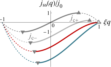
Figure 3: The current-momentum relation j ss ( q ) subscript 𝑗 ss 𝑞 j_{\rm ss}(q) ℰ ℰ {\mathcal{E}} j ss ( q ) / j 0 subscript 𝑗 ss 𝑞 subscript 𝑗 0 {j_{\rm ss}}(q)/j_{\rm 0} j 0 = 8 N 0 ξ 0 | ϵ ( ℰ ) | 3 / 2 / 3 3 β 0 subscript 𝑗 0 8 subscript 𝑁 0 subscript 𝜉 0 superscript italic-ϵ ℰ 3 2 3 3 subscript 𝛽 0 j_{\rm 0}=8N_{0}\xi_{0}|\epsilon({\mathcal{E}})|^{3/2}/3\sqrt{3}\beta_{0} ξ q 𝜉 𝑞 \xi q ξ q ℰ = 0 , 1 3 , 1 , 𝜉 subscript 𝑞 ℰ 0 1 3 1
\xi q_{\mathcal{E}}=0,\frac{1}{\sqrt{3}},1, 1.5 1.5 1.5 j c + subscript 𝑗 limit-from c {j_{\rm c+}} ξ q ℰ ≥ 1 𝜉 subscript 𝑞 ℰ 1 \xi q_{\mathcal{E}}\geq 1 j c − subscript 𝑗 limit-from c {j_{\rm c-}}
The current-momentum relation of the nonequilibrium steady state can be obtained by plugging the order parameter 𝝍 ( q , t ) = e i χ ss ( q , t ) R ss ( q ) ψ ^ ss ( q ) 𝝍 𝑞 𝑡 superscript 𝑒 𝑖 subscript 𝜒 ss 𝑞 𝑡 subscript 𝑅 ss 𝑞 subscript ^ 𝜓 ss 𝑞 \bm{\psi}(q,t)=e^{i\chi_{\rm ss}(q,t)}R_{\rm ss}(q)\hat{\psi}_{\rm ss}(q) 4
ψ ^ ss ( q ) ≃ ψ ^ eq ( q − a x θ ℰ / a y ′ ) , similar-to-or-equals subscript ^ 𝜓 ss 𝑞 subscript ^ 𝜓 eq 𝑞 subscript 𝑎 𝑥 subscript 𝜃 ℰ superscript subscript 𝑎 𝑦 ′ \hat{\psi}_{\rm ss}(q)\simeq\hat{\psi}_{\rm eq}(q-a_{x}\theta_{\mathcal{E}}/a_{y}^{\prime}), (10)
while the amplitude R ss ( q ) subscript 𝑅 ss 𝑞 R_{\rm ss}(q) a y ′ = ∂ q α y ( q ) | q → 0 superscript subscript 𝑎 𝑦 ′ evaluated-at subscript 𝑞 subscript 𝛼 𝑦 𝑞 → 𝑞 0 a_{y}^{\prime}=\partial_{q}\alpha_{y}(q)|_{q\to 0} [36 ] ,
the current-momentum relation of the steady state is given by,
j ss ( q ) = 4 N 0 ξ 0 2 β 0 ( q − q ℰ ) ( | ϵ ( ℰ ) | − ξ 0 2 q 2 ) , subscript 𝑗 ss 𝑞 4 subscript 𝑁 0 superscript subscript 𝜉 0 2 subscript 𝛽 0 𝑞 subscript 𝑞 ℰ italic-ϵ ℰ superscript subscript 𝜉 0 2 superscript 𝑞 2 {j_{\rm ss}}(q)=\frac{4N_{0}\xi_{0}^{2}}{\beta_{0}}(q-q_{\mathcal{E}})(|\epsilon({\mathcal{E}})|-\xi_{0}^{2}q^{2}), (11)
with the pumped momentum q ℰ = − a y ′ ℰ / 2 ξ 0 2 a x subscript 𝑞 ℰ superscript subscript 𝑎 𝑦 ′ ℰ 2 superscript subscript 𝜉 0 2 subscript 𝑎 𝑥 q_{\mathcal{E}}=-a_{y}^{\prime}{\mathcal{E}}/{2\xi_{0}^{2}a_{x}} q ℰ subscript 𝑞 ℰ q_{\mathcal{E}} [36 , 41 ] , and thus reflects the nonequilibrium nature of the steady state.
In Fig. 3 j ss ( q ) subscript 𝑗 ss 𝑞 j_{\rm ss}(q) ℰ ℰ {\mathcal{E}} j eq ( q ) subscript 𝑗 eq 𝑞 j_{\rm eq}(q) d j ss ( q ) / d q > 0 𝑑 subscript 𝑗 ss 𝑞 𝑑 𝑞 0 dj_{\rm ss}(q)/dq>0 [36 ] , which naturally generalizes the condition d j eq ( q ) / d q > 0 𝑑 subscript 𝑗 eq 𝑞 𝑑 𝑞 0 dj_{\rm eq}(q)/dq>0 [43 , 44 ] .
Interestingly, this does not coincide with the local-stability condition | ξ q | < 1 / 3 𝜉 𝑞 1 3 |\xi q|<1/\sqrt{3} [36 ] .
We find an interesting feature when focusing on the solid lines in Fig. 3 ℰ ℰ {\mathcal{E}} ℰ c2 ( ϵ ) subscript ℰ c2 italic-ϵ {\mathcal{E}_{\rm c2}}(\epsilon) j c + subscript 𝑗 limit-from c {j_{\rm c+}}
The onset electric field ℰ c2 ( ϵ ) subscript ℰ c2 italic-ϵ {\mathcal{E}_{\rm c2}}(\epsilon) | ξ q ℰ | = 1 𝜉 subscript 𝑞 ℰ 1 |\xi q_{\mathcal{E}}|=1 ℰ c2 ( ϵ ) subscript ℰ c2 italic-ϵ {\mathcal{E}_{\rm c2}}(\epsilon) ℰ c ( ϵ ) subscript ℰ c italic-ϵ {\mathcal{E}_{\rm c}}(\epsilon) [36 ] ,
ℰ c2 ( ϵ ) ℰ c ( ϵ ) = 1 1 + 𝒞 2 ≤ 1 , subscript ℰ c2 italic-ϵ subscript ℰ c italic-ϵ 1 1 superscript 𝒞 2 1 \frac{{\mathcal{E}_{\rm c2}}(\epsilon)}{{\mathcal{E}_{\rm c}}(\epsilon)}=\frac{1}{\sqrt{1+{\mathcal{C}}^{2}}}\leq 1, (12)
where we defined
𝒞 ≡ ξ 0 d q ℰ d ℰ ℰ c | ϵ → − 1 = ± | ξ 0 − 1 a y ′ | 2 | a x | , 𝒞 evaluated-at subscript 𝜉 0 𝑑 subscript 𝑞 ℰ 𝑑 ℰ subscript ℰ c → italic-ϵ 1 plus-or-minus superscript subscript 𝜉 0 1 superscript subscript 𝑎 𝑦 ′ 2 subscript 𝑎 𝑥 {\mathcal{C}}\equiv\xi_{0}\frac{dq_{\mathcal{E}}}{d{\mathcal{E}}}\left.{\mathcal{E}_{\rm c}}\right|_{\epsilon\to-1}={\pm\frac{|\xi_{0}^{-1}a_{y}^{\prime}|}{\sqrt{2|a_{x}|}},} (13)
with ± = sgn [ − a x a y ′ ] \pm=\mathrm{sgn}\,[-a_{x}a_{y}^{\prime}] 12
The dimensionless constant 𝒞 𝒞 {\mathcal{C}} LABEL:fig:phasediagram (a) the phase diagram for 𝒞 = 1 𝒞 1 {\mathcal{C}}=1 0.8 ≤ T / T c0 ≤ 1 0.8 𝑇 subscript 𝑇 c0 1 0.8\leq T/{T_{\rm c0}}\leq 1 η ≡ ( j c + − j c − ) / ( j c + + j c − ) 𝜂 subscript 𝑗 limit-from c subscript 𝑗 limit-from c subscript 𝑗 limit-from c subscript 𝑗 limit-from c \eta\equiv({j_{\rm c+}}-{j_{\rm c-}})/({j_{\rm c+}}+{j_{\rm c-}}) ℰ c2 ( ϵ ) ≤ ℰ ≤ ℰ c ( ϵ ) subscript ℰ c2 italic-ϵ ℰ subscript ℰ c italic-ϵ {\mathcal{E}}_{\rm c2}(\epsilon)\leq{\mathcal{E}}\leq{\mathcal{E}}_{\rm c}(\epsilon) | η | = 1 𝜂 1 |\eta|=1 ℰ c2 ( ϵ ) subscript ℰ c2 italic-ϵ {\mathcal{E}_{\rm c2}}(\epsilon) LABEL:fig:phasediagram (b) the evolution of η 𝜂 \eta 𝒞 𝒞 {\mathcal{C}} ℰ ℰ {\mathcal{E}} 𝒞 ≳ 0.5 greater-than-or-equivalent-to 𝒞 0.5 {\mathcal{C}}\gtrsim 0.5 η 𝜂 \eta ℰ ℰ \mathcal{E}
η 𝜂 \displaystyle\eta = − 3 𝒞 ℰ ℰ c ( ϵ ) + O ( ℰ 2 ) , absent 3 𝒞 ℰ subscript ℰ c italic-ϵ 𝑂 superscript ℰ 2 \displaystyle=-\sqrt{3}\,{\mathcal{C}}\,\frac{{\mathcal{E}}}{{\mathcal{E}}_{\rm c}(\epsilon)}+O\left({{\mathcal{E}}}^{2}\right), (14)
describing the dissipation-induced SDE.
This is O ( | ϵ | 0 ) 𝑂 superscript italic-ϵ 0 O(|\epsilon|^{0}) O ( | ϵ | 1 / 2 ) 𝑂 superscript italic-ϵ 1 2 O(|\epsilon|^{1/2}) [8 , 9 , 10 , 11 , 12 ] .
Discussion. — Our results are straightforwardly generalized to arbitrary bilayer GL model [36 ] .
In particular,
the steady state ψ ^ ss ( q ) subscript ^ 𝜓 ss 𝑞 \hat{\psi}_{\rm ss}(q) α ^ eff ( q ) subscript ^ 𝛼 eff 𝑞 \hat{\alpha}_{\rm eff}(q) O ( | ϵ | ) 𝑂 italic-ϵ O(|\epsilon|) 11 ϵ ( ℰ ) italic-ϵ ℰ \epsilon({\mathcal{E}}) ξ 0 2 superscript subscript 𝜉 0 2 \xi_{0}^{2} β 0 subscript 𝛽 0 \beta_{0} q ℰ subscript 𝑞 ℰ q_{\mathcal{E}} 𝒞 𝒞 \mathcal{C}
The GL coefficient a y ′ = ∂ q α y ( q ) | q → 0 superscript subscript 𝑎 𝑦 ′ evaluated-at subscript 𝑞 subscript 𝛼 𝑦 𝑞 → 𝑞 0 a_{y}^{\prime}=\partial_{q}\alpha_{y}(q)|_{q\to 0} 𝒞 𝒞 \mathcal{C} C 2 h subscript 𝐶 2 ℎ C_{2h} D 3 d subscript 𝐷 3 𝑑 D_{3d} [45 , 46 ] ,
and superconductivity has been observed in atomically-thin MoS2 [47 , 48 , 49 ] and NbSe2 [50 , 51 , 52 , 53 , 54 ] ,
for example.
Bernal-stacked bilayer graphene [55 , 56 , 57 , 58 , 59 ] and Lix [60 , 61 , 62 ]
also have D 3 d subscript 𝐷 3 𝑑 D_{3d} D 3 d subscript 𝐷 3 𝑑 D_{3d} C 2 h subscript 𝐶 2 ℎ C_{2h} [46 ] or with nematic orders [57 , 58 , 59 ] are the experimental platform of the
USC.
To obtain a large conversion efficiency 𝒞 𝒞 {\mathcal{C}} ξ 0 subscript 𝜉 0 \xi_{0} [63 , 64 , 65 , 66 ] and heavy-fermion superlattices [67 , 68 ] ,
as well as systems near a pair-density-wave transition with small | a x | subscript 𝑎 𝑥 |a_{x}| [38 , 37 ] , are suitable once the symmetry requirement is satisfied.
The actual current-resistivity relation may differ from our results for various reasons.
While j c − subscript 𝑗 limit-from c j_{\rm c-} 3 14 j c + subscript 𝑗 limit-from c j_{\rm c+} 1 3
Conclusion. —
In this Letter, we have proposed a setup to realize USC: applying the out-of-plane electric field and current to a wire or thin film of bilayer superconductors lacking the in-plane inversion symmetry.
The inter-layer phase difference θ ℰ subscript 𝜃 ℰ \theta_{\mathcal{E}} a y ′ = ∂ q α y ( q ) | q → 0 superscript subscript 𝑎 𝑦 ′ evaluated-at subscript 𝑞 subscript 𝛼 𝑦 𝑞 → 𝑞 0 a_{y}^{\prime}=\partial_{q}\alpha_{y}(q)|_{q\to 0} 100 % percent 100 100\% [5 ] is left unclear, but
dissipation could be important as illustrated in this Letter.
Acknowledgements.
We thank Hikaru Watanabe and Kazuaki Takasan for their helpful discussions.
This work was supported by JSPS KAKENHI (Grant Nos. JP21K13880, JP21K18145, JP22H01181, JP22H04476, JP22H04933, JP23K17353).
References
Ando et al. [2020]
F. Ando, Y. Miyasaka,
T. Li, J. Ishizuka, T. Arakawa, Y. Shiota, T. Moriyama, Y. Yanase, and T. Ono, Nature 584 , 373 (2020) .
Wu et al. [2022]
H. Wu, Y. Wang, Y. Xu, P. K. Sivakumar, C. Pasco, U. Filippozzi, S. S. P. Parkin, Y.-J. Zeng, T. McQueen, and M. N. Ali, Nature 604 , 653 (2022) .
Bauriedl et al. [2022]
L. Bauriedl, C. Bäuml,
L. Fuchs, C. Baumgartner, N. Paulik, J. M. Bauer, K.-Q. Lin, J. M. Lupton, T. Taniguchi,
K. Watanabe, C. Strunk, and N. Paradiso, Nat.
Commun. 13 , 4266
(2022) .
Narita et al. [2022]
H. Narita, J. Ishizuka,
R. Kawarazaki, D. Kan, Y. Shiota, T. Moriyama, Y. Shimakawa, A. V. Ognev, A. S. Samardak, Y. Yanase, and T. Ono, Nat. Nanotechnol. 17 , 823 (2022) .
Lin et al. [2022]
J.-X. Lin, P. Siriviboon,
H. D. Scammell, S. Liu, D. Rhodes, K. Watanabe, T. Taniguchi, J. Hone, M. S. Scheurer, and J. I. A. Li, Nat. Phys. 18 , 1221 (2022) .
Yun et al. [2023]
J. Yun, S. Son, J. Shin, G. Park, K. Zhang, Y. J. Shin, J.-G. Park, and D. Kim, Phys. Rev. Res. 5 , L022064 (2023) .
Scammell et al. [2022]
H. D. Scammell, J. I. A. Li,
and M. S. Scheurer, 2D Mater. 9 , 025027 (2022) .
Yuan and Fu [2022]
N. F. Q. Yuan and L. Fu, Proceedings of the National Academy of Sciences 119 , e2119548119 (2022) , arXiv:2106.01909
[cond-mat.supr-con] .
Daido et al. [2022]
A. Daido, Y. Ikeda, and Y. Yanase, Phys. Rev. Lett. 128 , 037001 (2022) .
He et al. [2022]
J. J. He, Y. Tanaka, and N. Nagaosa, New J. Phys. 24 , 053014 (2022) .
Ilić and Bergeret [2022]
S. Ilić and F. S. Bergeret, Phys. Rev. Lett. 128 , 177001 (2022) .
Daido and Yanase [2022]
A. Daido and Y. Yanase, Phys. Rev. B Condens. Matter 106 , 205206 (2022) .
Jiang et al. [1994]
X. Jiang, P. J. Connolly,
S. J. Hagen, and C. J. Lobb, Phys. Rev. B Condens. Matter 49 , 9244 (1994) .
Ichikawa et al. [1994]
F. Ichikawa, T. Nishizaki,
K. Yamabe, Y. Yamasaki, T. Fukami, and T. Aomine, Physica C Supercond. 235-240 , 3095 (1994) .
Vodolazov and Peeters [2005]
D. Y. Vodolazov and F. M. Peeters, Phys. Rev. B Condens. Matter 72 , 172508 (2005) .
Harrington et al. [2009]
S. A. Harrington, J. L. MacManus-Driscoll, and J. H. Durrell, Appl. Phys. Lett. 95 , 022518 (2009) .
Lyu et al. [2021]
Y.-Y. Lyu, J. Jiang, Y.-L. Wang, Z.-L. Xiao, S. Dong, Q.-H. Chen, M. V. Milošević, H. Wang, R. Divan, J. E. Pearson,
P. Wu, F. M. Peeters, and W.-K. Kwok, Nat.
Commun. 12 , 2703
(2021) .
Hou et al. [2023]
Y. Hou, F. Nichele,
H. Chi, A. Lodesani, Y. Wu, M. F. Ritter, D. Z. Haxell, M. Davydova, S. Ilić,
O. Glezakou-Elbert,
A. Varambally, F. S. Bergeret, A. Kamra, L. Fu, P. A. Lee, and J. S. Moodera, Phys. Rev. Lett. 131 , 027001 (2023) .
Mizuno et al. [2022]
A. Mizuno, Y. Tsuchiya,
S. Awaji, and Y. Yoshida, IEEE
Trans. Appl. Supercond. 32 , 1 (2022) .
Tokura and Nagaosa [2018]
Y. Tokura and N. Nagaosa, Nat. Commun. 9 , 3740 (2018) .
Ideue and Iwasa [2021]
T. Ideue and Y. Iwasa, Annu. Rev. Condens. Matter Phys. 12 , 201 (2021) .
Wakatsuki et al. [2017]
R. Wakatsuki, Y. Saito,
S. Hoshino, Y. M. Itahashi, T. Ideue, M. Ezawa, Y. Iwasa, and N. Nagaosa, Science Advances 3 , e1602390 (2017) .
Wakatsuki and Nagaosa [2018]
R. Wakatsuki and N. Nagaosa, Phys. Rev. Lett. 121 , 026601 (2018) .
Hoshino et al. [2018]
S. Hoshino, R. Wakatsuki,
K. Hamamoto, and N. Nagaosa, Phys. Rev. B Condens. Matter 98 , 054510 (2018) .
Qin et al. [2017]
F. Qin, W. Shi, T. Ideue, M. Yoshida, A. Zak, R. Tenne, T. Kikitsu,
D. Inoue, D. Hashizume, and Y. Iwasa, Nat.
Commun. 8 , 14465
(2017) .
Yasuda et al. [2019]
K. Yasuda, H. Yasuda,
T. Liang, R. Yoshimi, A. Tsukazaki, K. S. Takahashi, N. Nagaosa, M. Kawasaki, and Y. Tokura, Nat. Commun. 10 , 2734 (2019) .
Zhang et al. [2020]
E. Zhang, X. Xu, Y.-C. Zou, L. Ai, X. Dong, C. Huang, P. Leng,
S. Liu, Y. Zhang, Z. Jia, X. Peng, M. Zhao, Y. Yang, Z. Li, H. Guo, S. J. Haigh, N. Nagaosa, J. Shen, and F. Xiu, Nat. Commun. 11 , 5634 (2020) .
Daido and Yanase [2023]
A. Daido and Y. Yanase, (2023), arXiv:2302.10677 [cond-mat.supr-con]
.
Bohm [1949]
D. Bohm, Phys. Rev. 75 , 502 (1949) .
Ohashi and Momoi [1996]
Y. Ohashi and T. Momoi, J. Phys. Soc. Jpn. 65 , 3254 (1996) .
Watanabe [2019]
H. Watanabe, J. Stat. Phys. 177 , 717 (2019) .
Tinkham [2004]
M. Tinkham, Introduction to
Superconductivity (Courier Corporation, 2004).
Kopnin [2001]
N. B. Kopnin, Theory of Nonequilibrium
Superconductivity (Clarendon Press, 2001).
Artemenko and Volkov [1979]
S. N. Artemenko and A. F. Volkov, Sov. Phys. Usp. 22 , 295 (1979) .
Fruchart et al. [2021]
M. Fruchart, R. Hanai,
P. B. Littlewood, and V. Vitelli, Nature 592 , 363 (2021) .
[36]
See Supplemental Material.
Khim et al. [2021]
S. Khim, J. F. Landaeta,
J. Banda, N. Bannor, M. Brando, P. M. R. Brydon, D. Hafner, R. Küchler, R. Cardoso-Gil, U. Stockert, A. P. Mackenzie, D. F. Agterberg, C. Geibel, and E. Hassinger, Science 373 , 1012 (2021) .
Fischer et al. [2023]
M. H. Fischer, M. Sigrist,
D. F. Agterberg, and Y. Yanase, Annu. Rev. Condens. Matter Phys. (2023), 10.1146/annurev-conmatphys-040521-042511 .
Rubinstein et al. [2007]
J. Rubinstein, P. Sternberg, and Q. Ma, Phys. Rev. Lett. 99 , 167003 (2007) .
Chtchelkatchev et al. [2012]
N. M. Chtchelkatchev, A. A. Golubov, T. I. Baturina, and V. M. Vinokur, Phys. Rev. Lett. 109 , 150405 (2012) .
Ashida et al. [2020]
Y. Ashida, Z. Gong, and M. Ueda, Adv. Phys. 69 , 249
(2020) .
Larkin and Varlamov [2005]
A. Larkin and A. Varlamov, Theory of Fluctuations
in Superconductors (OUP Oxford, 2005).
Langer and Ambegaokar [1967]
J. S. Langer and V. Ambegaokar, Phys. Rev. 164 , 498 (1967) .
Samokhin and Truong [2017]
K. V. Samokhin and B. P. Truong, Phys. Rev. B Condens. Matter 96 , 214501 (2017) .
Liu et al. [2015]
G.-B. Liu, D. Xiao, Y. Yao, X. Xu, and W. Yao, Chem. Soc.
Rev. 44 , 2643 (2015) .
Manzeli et al. [2017]
S. Manzeli, D. Ovchinnikov, D. Pasquier, O. V. Yazyev, and A. Kis, Nature Reviews Materials 2 , 1 (2017) .
Ye et al. [2012]
J. T. Ye, Y. J. Zhang,
R. Akashi, M. S. Bahramy, R. Arita, and Y. Iwasa, Science 338 , 1193
(2012) .
Saito et al. [2015]
Y. Saito, Y. Nakamura,
M. S. Bahramy, Y. Kohama, J. Ye, Y. Kasahara, Y. Nakagawa, M. Onga, M. Tokunaga, T. Nojima,
Y. Yanase, and Y. Iwasa, Nat. Phys. 12 , 144 (2015) .
Lu et al. [2015]
J. M. Lu, O. Zheliuk,
I. Leermakers, N. F. Q. Yuan, U. Zeitler, K. T. Law, and J. T. Ye, Science 350 , 1353 (2015) .
Frindt [1972]
R. F. Frindt, Phys. Rev. Lett. 28 , 299 (1972) .
Staley et al. [2009]
N. E. Staley, J. Wu, P. Eklund, Y. Liu, L. Li, and Z. Xu, Phys. Rev. B Condens. Matter 80 , 184505 (2009) .
Cao et al. [2015]
Y. Cao, A. Mishchenko,
G. L. Yu, E. Khestanova, A. P. Rooney, E. Prestat, A. V. Kretinin, P. Blake, M. B. Shalom, C. Woods, J. Chapman,
G. Balakrishnan, I. V. Grigorieva, K. S. Novoselov, B. A. Piot, M. Potemski, K. Watanabe, T. Taniguchi, S. J. Haigh, A. K. Geim, and R. V. Gorbachev, Nano Lett. 15 , 4914
(2015) .
Xi et al. [2015a]
X. Xi, L. Zhao, Z. Wang, H. Berger, L. Forró, J. Shan, and K. F. Mak, Nat. Nanotechnol. 10 , 765 (2015a) .
Xi et al. [2015b]
X. Xi, Z. Wang, W. Zhao, J.-H. Park, K. T. Law, H. Berger, L. Forró, J. Shan, and K. F. Mak, Nat. Phys. 12 , 139 (2015b) .
McCann and Koshino [2013]
E. McCann and M. Koshino, Rep. Prog. Phys. 76 , 056503 (2013) .
de la Barrera et al. [2022]
S. C. de la Barrera, S. Aronson, Z. Zheng,
K. Watanabe, T. Taniguchi, Q. Ma, P. Jarillo-Herrero, and R. Ashoori, Nat. Phys. 18 , 771 (2022) .
Zhou et al. [2022]
H. Zhou, L. Holleis,
Y. Saito, L. Cohen, W. Huynh, C. L. Patterson, F. Yang, T. Taniguchi, K. Watanabe,
and A. F. Young, Science 375 , 774 (2022) .
Zhang et al. [2023]
Y. Zhang, R. Polski,
A. Thomson, É. Lantagne-Hurtubise, C. Lewandowski, H. Zhou, K. Watanabe, T. Taniguchi, J. Alicea, and S. Nadj-Perge, Nature 613 , 268
(2023) .
Dong et al. [2023]
Z. Dong, M. Davydova,
O. Ogunnaike, and L. Levitov, Phys. Rev. B Condens. Matter 107 , 075108 (2023) .
Kasahara et al. [2015]
Y. Kasahara, K. Kuroki,
S. Yamanaka, and Y. Taguchi, Phys. C 514 , 354 (2015) .
Nakagawa et al. [2018]
Y. Nakagawa, Y. Saito,
T. Nojima, K. Inumaru, S. Yamanaka, Y. Kasahara, and Y. Iwasa, Phys.
Rev. B Condens. Matter 98 , 064512 (2018) .
Nakagawa et al. [2021]
Y. Nakagawa, Y. Kasahara,
T. Nomoto, R. Arita, T. Nojima, and Y. Iwasa, Science 372 , 190
(2021) .
Cao et al. [2018]
Y. Cao, V. Fatemi,
S. Fang, K. Watanabe, T. Taniguchi, E. Kaxiras, and P. Jarillo-Herrero, Nature 556 , 43 (2018) .
Park et al. [2021]
J. M. Park, Y. Cao, K. Watanabe, T. Taniguchi, and P. Jarillo-Herrero, Nature 590 , 249
(2021) .
Hao et al. [2021]
Z. Hao, A. M. Zimmerman,
P. Ledwith, E. Khalaf, D. H. Najafabadi, K. Watanabe, T. Taniguchi, A. Vishwanath, and P. Kim, Science 371 , 1133
(2021) .
Park et al. [2022]
J. M. Park, Y. Cao, L.-Q. Xia, S. Sun, K. Watanabe, T. Taniguchi, and P. Jarillo-Herrero, Nat.
Mater. 21 , 877 (2022) .
Mizukami et al. [2011]
Y. Mizukami, H. Shishido,
T. Shibauchi, M. Shimozawa, S. Yasumoto, D. Watanabe, M. Yamashita, H. Ikeda, T. Terashima, H. Kontani, and Y. Matsuda, Nat. Phys. 7 , 849 (2011) .
Naritsuka et al. [2021]
M. Naritsuka, T. Terashima, and Y. Matsuda, J. Phys. Condens. Matter 33 , 273001 (2021) .
I Symmetry requirements of α y ( q ) subscript 𝛼 𝑦 𝑞 \alpha_{y}(q)
In this section, we discuss the symmetry requirements to obtain a finite a y ′ = ∂ q α y ( q ) | q → 0 superscript subscript 𝑎 𝑦 ′ evaluated-at subscript 𝑞 subscript 𝛼 𝑦 𝑞 → 𝑞 0 a_{y}^{\prime}=\partial_{q}\alpha_{y}(q)|_{q\to 0} σ y subscript 𝜎 𝑦 \sigma_{y}
σ y subscript 𝜎 𝑦 \displaystyle\sigma_{y} ∼ − i | z = d / 2 ⟩ ⟨ z = − d / 2 | similar-to absent 𝑖 ket 𝑧 𝑑 2 bra 𝑧 𝑑 2 \displaystyle\sim-i\ket{z=d/2}\bra{z=-d/2}
+ i | z = − d / 2 ⟩ ⟨ z = d / 2 | , 𝑖 ket 𝑧 𝑑 2 bra 𝑧 𝑑 2 \displaystyle\qquad\qquad+i\ket{z=-d/2}\bra{z=d/2}, (15)
which is symmetry-equivalent to the momentum operator in the z 𝑧 z d 𝑑 d a y ′ superscript subscript 𝑎 𝑦 ′ a_{y}^{\prime}
a y ′ ∼ k x k z , similar-to superscript subscript 𝑎 𝑦 ′ subscript 𝑘 𝑥 subscript 𝑘 𝑧 \displaystyle a_{y}^{\prime}\sim k_{x}k_{z}, (16)
which must belong to the identity representation of the point group.
The rotation axis can exist only in the y 𝑦 y C 2 v subscript 𝐶 2 𝑣 C_{2v} k x k z subscript 𝑘 𝑥 subscript 𝑘 𝑧 k_{x}k_{z} C 2 v subscript 𝐶 2 𝑣 C_{2v} a y ′ superscript subscript 𝑎 𝑦 ′ a_{y}^{\prime} C 2 h subscript 𝐶 2 ℎ C_{2h} y 𝑦 y C 1 subscript 𝐶 1 C_{1} C i subscript 𝐶 𝑖 C_{i} C s subscript 𝐶 𝑠 C_{s} C 2 subscript 𝐶 2 C_{2} a y ′ superscript subscript 𝑎 𝑦 ′ a_{y}^{\prime}
II The bilayer TDGL model
II.1 Bilayer TDGL model under electromagnetic fields
Here we introduce the electric field to the bilayer TDGL equation.
The TDGL equation is given by
Γ N 0 ∂ t 𝝍 ( x , t ) = − [ α ^ ( ∇ / i ) + β 0 𝝍 † ( x , t ) 𝝍 ( x , t ) ] 𝝍 ( x , t ) , Γ subscript 𝑁 0 subscript 𝑡 𝝍 𝑥 𝑡 delimited-[] ^ 𝛼 ∇ 𝑖 subscript 𝛽 0 superscript 𝝍 † 𝑥 𝑡 𝝍 𝑥 𝑡 𝝍 𝑥 𝑡 \displaystyle\!\!\!\!\!\!\!\!\frac{\Gamma}{N_{0}}\partial_{t}\bm{\psi}(x,t)=-[\hat{\alpha}(\nabla/i)+\beta_{0}\bm{\psi}^{\dagger}(x,t)\bm{\psi}(x,t)]\bm{\psi}(x,t), (17)
in the absence of electromagnetic fields.
By gauge transformation, the order parameter transforms by
ψ i ′ ( x , t ) = e − 2 i χ i ( x , t ) ψ i ( x , t ) , subscript superscript 𝜓 ′ 𝑖 𝑥 𝑡 superscript 𝑒 2 𝑖 subscript 𝜒 𝑖 𝑥 𝑡 subscript 𝜓 𝑖 𝑥 𝑡 \displaystyle{\psi}^{\prime}_{i}(x,t)=e^{-2i\chi_{i}(x,t)}\psi_{i}(x,t), (18)
or equivalently,
𝝍 ′ ( x , t ) = e − 2 i χ ¯ ( x , t ) e − i δ χ ( x , t ) σ z 𝝍 ( x , t ) , superscript 𝝍 ′ 𝑥 𝑡 superscript 𝑒 2 𝑖 ¯ 𝜒 𝑥 𝑡 superscript 𝑒 𝑖 𝛿 𝜒 𝑥 𝑡 subscript 𝜎 𝑧 𝝍 𝑥 𝑡 \displaystyle\bm{\psi}^{\prime}(x,t)=e^{-2i\bar{\chi}(x,t)}e^{-i\delta\chi(x,t)\sigma_{z}}\bm{\psi}(x,t), (19)
with
χ ¯ ( x , t ) ¯ 𝜒 𝑥 𝑡 \displaystyle\bar{\chi}(x,t) ≡ χ 1 ( x , t ) + χ 2 ( x , t ) 2 , absent subscript 𝜒 1 𝑥 𝑡 subscript 𝜒 2 𝑥 𝑡 2 \displaystyle\equiv\frac{\chi_{1}(x,t)+\chi_{2}(x,t)}{2}, (20a)
δ χ ( x , t ) 𝛿 𝜒 𝑥 𝑡 \displaystyle\delta{\chi}(x,t) ≡ χ 1 ( x , t ) − χ 2 ( x , t ) . absent subscript 𝜒 1 𝑥 𝑡 subscript 𝜒 2 𝑥 𝑡 \displaystyle\equiv{\chi_{1}(x,t)-\chi_{2}(x,t)}. (20b)
The transformed order parameter satisfies
Γ N 0 [ ∂ t + 2 i ∂ t χ ¯ ( x , t ) + i ∂ t δ χ ( x , t ) σ z ] ψ i ′ ( x , t ) Γ subscript 𝑁 0 delimited-[] subscript 𝑡 2 𝑖 subscript 𝑡 ¯ 𝜒 𝑥 𝑡 𝑖 subscript 𝑡 𝛿 𝜒 𝑥 𝑡 subscript 𝜎 𝑧 superscript subscript 𝜓 𝑖 ′ 𝑥 𝑡 \displaystyle\frac{\Gamma}{N_{0}}[\partial_{t}+2i\partial_{t}\bar{\chi}(x,t)+i\partial_{t}\delta\chi(x,t)\sigma_{z}]\psi_{i}^{\prime}(x,t)
= − e − i δ χ ( x , t ) σ z [ α ^ ( ∇ / i + 2 ∇ χ ¯ ) \displaystyle=-e^{-i\delta\chi(x,t)\sigma_{z}}[\hat{\alpha}(\nabla/i+2\nabla\bar{\chi})
+ β 0 𝝍 ′ † ( x , t ) 𝝍 ′ ( x , t ) ] e i δ χ ( x , t ) σ z 𝝍 ′ ( x , t ) . \displaystyle\qquad+\beta_{0}\bm{\psi}^{\prime\dagger}(x,t)\bm{\psi}^{\prime}(x,t)]e^{i\delta\chi(x,t)\sigma_{z}}\bm{\psi}^{\prime}(x,t). (21)
The electromagnetic field should be incorporated into the equation to cancel the terms dependent on χ i ( x , t ) subscript 𝜒 𝑖 𝑥 𝑡 \chi_{i}(x,t) 𝑨 ( x , z , t ) 𝑨 𝑥 𝑧 𝑡 \bm{A}(x,z,t) ϕ ( x , z , t ) italic-ϕ 𝑥 𝑧 𝑡 \phi(x,z,t)
δ A ( x , t ) 𝛿 𝐴 𝑥 𝑡 \displaystyle\delta A(x,t) ≡ ∫ − d / 2 d / 2 𝑑 z A z ( x , z , t ) absent superscript subscript 𝑑 2 𝑑 2 differential-d 𝑧 subscript 𝐴 𝑧 𝑥 𝑧 𝑡 \displaystyle\equiv\int_{-d/2}^{d/2}dz\,A_{z}(x,z,t)
→ δ A ′ ( x , t ) → absent 𝛿 superscript 𝐴 ′ 𝑥 𝑡 \displaystyle\to\delta A^{\prime}(x,t) = ∫ − d / 2 d / 2 𝑑 z A z ( x , z , t ) − ∂ z χ ( x , z , t ) absent superscript subscript 𝑑 2 𝑑 2 differential-d 𝑧 subscript 𝐴 𝑧 𝑥 𝑧 𝑡 subscript 𝑧 𝜒 𝑥 𝑧 𝑡 \displaystyle=\int_{-d/2}^{d/2}dz\,A_{z}(x,z,t)-\partial_{z}\chi(x,z,t)
= δ A ( x , t ) − δ χ ( x , t ) , absent 𝛿 𝐴 𝑥 𝑡 𝛿 𝜒 𝑥 𝑡 \displaystyle=\delta A(x,t)-\delta\chi(x,t), (22a)
A ¯ ( x , t ) ¯ 𝐴 𝑥 𝑡 \displaystyle\bar{A}(x,t) ≡ A x ( x , d / 2 , t ) + A x ( x , − d / 2 , t ) 2 absent subscript 𝐴 𝑥 𝑥 𝑑 2 𝑡 subscript 𝐴 𝑥 𝑥 𝑑 2 𝑡 2 \displaystyle\equiv\frac{A_{x}(x,d/2,t)+A_{x}(x,-d/2,t)}{2}
→ A ¯ ′ ( x , t ) → absent superscript ¯ 𝐴 ′ 𝑥 𝑡 \displaystyle\to\bar{A}^{\prime}(x,t) = A ¯ ( x , t ) − ∇ χ ¯ ( x , t ) , absent ¯ 𝐴 𝑥 𝑡 ∇ ¯ 𝜒 𝑥 𝑡 \displaystyle=\bar{A}(x,t)-\nabla\bar{\chi}(x,t), (22b)
δ ϕ ( x , t ) 𝛿 italic-ϕ 𝑥 𝑡 \displaystyle\delta\phi(x,t) ≡ ϕ ( x , d / 2 , t ) − ϕ ( x , − d / 2 , t ) absent italic-ϕ 𝑥 𝑑 2 𝑡 italic-ϕ 𝑥 𝑑 2 𝑡 \displaystyle\equiv\phi(x,d/2,t)-\phi(x,-d/2,t)
→ δ ϕ ′ ( x , t ) → absent 𝛿 superscript italic-ϕ ′ 𝑥 𝑡 \displaystyle\to\delta\phi^{\prime}(x,t) = δ ϕ ( x , t ) + ∂ t δ χ ( x , t ) , absent 𝛿 italic-ϕ 𝑥 𝑡 subscript 𝑡 𝛿 𝜒 𝑥 𝑡 \displaystyle=\delta\phi(x,t)+\partial_{t}\delta\chi(x,t), (22c)
ϕ ¯ ( x , t ) ¯ italic-ϕ 𝑥 𝑡 \displaystyle\bar{\phi}(x,t) ≡ ϕ ( x , d / 2 , t ) + ϕ ( x , − d / 2 , t ) 2 absent italic-ϕ 𝑥 𝑑 2 𝑡 italic-ϕ 𝑥 𝑑 2 𝑡 2 \displaystyle\equiv\frac{\phi(x,d/2,t)+\phi(x,-d/2,t)}{2}
→ ϕ ¯ ′ ( x , t ) → absent superscript ¯ italic-ϕ ′ 𝑥 𝑡 \displaystyle\to\bar{\phi}^{\prime}(x,t) = ϕ ¯ ( x , t ) + ∂ t χ ¯ ( x , t ) , absent ¯ italic-ϕ 𝑥 𝑡 subscript 𝑡 ¯ 𝜒 𝑥 𝑡 \displaystyle=\bar{\phi}(x,t)+\partial_{t}\bar{\chi}(x,t), (22d)
by using χ 1 ( x , t ) = χ ( x , d / 2 , t ) subscript 𝜒 1 𝑥 𝑡 𝜒 𝑥 𝑑 2 𝑡 \chi_{1}(x,t)=\chi(x,d/2,t) χ 2 ( x , t ) = χ ( x , − d / 2 , t ) subscript 𝜒 2 𝑥 𝑡 𝜒 𝑥 𝑑 2 𝑡 \chi_{2}(x,t)=\chi(x,-d/2,t) 𝑨 = 0 𝑨 0 \bm{A}=0 ϕ = 0 italic-ϕ 0 \phi=0 χ ¯ ¯ 𝜒 \bar{\chi} δ χ 𝛿 𝜒 \delta\chi 𝑨 ′ superscript 𝑨 ′ \bm{A}^{\prime} ϕ ′ superscript italic-ϕ ′ \phi^{\prime}
Γ N 0 [ ∂ t + 2 i ϕ ¯ ( x , t ) + i δ ϕ ( x , t ) σ z ] 𝝍 ( x , t ) Γ subscript 𝑁 0 delimited-[] subscript 𝑡 2 𝑖 ¯ italic-ϕ 𝑥 𝑡 𝑖 𝛿 italic-ϕ 𝑥 𝑡 subscript 𝜎 𝑧 𝝍 𝑥 𝑡 \displaystyle\frac{\Gamma}{N_{0}}\left[\partial_{t}+2i\bar{\phi}(x,t)+i\delta\phi(x,t)\sigma_{z}\right]\bm{\psi}(x,t)
= − e i δ A ( x , t ) σ z [ α ^ ( ∇ / i − 2 A ¯ ( x , t ) ) \displaystyle=-e^{i\delta A(x,t)\sigma_{z}}[\hat{\alpha}(\nabla/i-2\bar{A}(x,t))
+ β 0 𝝍 † ( x , t ) 𝝍 ( x , t ) ] e − i δ A ( x , t ) σ z 𝝍 ( x , t ) , \displaystyle\qquad+\beta_{0}\bm{\psi}^{\dagger}(x,t)\bm{\psi}(x,t)]e^{-i\delta A(x,t)\sigma_{z}}\bm{\psi}(x,t), (23)
where we removed the prime of the quantities.
We adopt the gauge where the vector potential vanishes and describe the perpendicular electric field by the scalar potential ϕ ( z ) = − E ⟂ z italic-ϕ 𝑧 subscript 𝐸 perpendicular-to 𝑧 \phi(z)=-E_{\perp}z δ ϕ = − E ⟂ d 𝛿 italic-ϕ subscript 𝐸 perpendicular-to 𝑑 \delta\phi=-E_{\perp}d
Γ N 0 [ ∂ t − i E ⟂ d σ z ] 𝝍 ( x , t ) Γ subscript 𝑁 0 delimited-[] subscript 𝑡 𝑖 subscript 𝐸 perpendicular-to 𝑑 subscript 𝜎 𝑧 𝝍 𝑥 𝑡 \displaystyle\frac{\Gamma}{N_{0}}\left[\partial_{t}-iE_{\perp}d\sigma_{z}\right]\bm{\psi}(x,t)
= − [ α ^ ( ∇ / i ) + β 0 𝝍 † ( x , t ) 𝝍 ( x , t ) ] 𝝍 ( x , t ) , absent delimited-[] ^ 𝛼 ∇ 𝑖 subscript 𝛽 0 superscript 𝝍 † 𝑥 𝑡 𝝍 𝑥 𝑡 𝝍 𝑥 𝑡 \displaystyle=-[\hat{\alpha}(\nabla/i)+\beta_{0}\bm{\psi}^{\dagger}(x,t)\bm{\psi}(x,t)]\bm{\psi}(x,t), (24)
which gives
[ ∂ t + i Φ ] 𝝍 ( q , t ) = − [ α ^ ( q ) + β 0 | 𝝍 ( q , t ) | 2 ] 𝝍 ( q , t ) , delimited-[] subscript 𝑡 𝑖 Φ 𝝍 𝑞 𝑡 delimited-[] ^ 𝛼 𝑞 subscript 𝛽 0 superscript 𝝍 𝑞 𝑡 2 𝝍 𝑞 𝑡 \displaystyle\left[\partial_{t}+i\Phi\right]\bm{\psi}(q,t)=-[\hat{\alpha}(q)+\beta_{0}|\bm{\psi}(q,t)|^{2}]\bm{\psi}(q,t), (25)
with t → Γ t / N 0 → 𝑡 Γ 𝑡 subscript 𝑁 0 t\to\Gamma t/N_{0} Φ = − Γ E ⟂ d σ z / N 0 Φ Γ subscript 𝐸 perpendicular-to 𝑑 subscript 𝜎 𝑧 subscript 𝑁 0 \Phi=-\Gamma E_{\perp}d\sigma_{z}/N_{0} 𝝍 ( x , t ) = e i q x 𝝍 ( q , t ) 𝝍 𝑥 𝑡 superscript 𝑒 𝑖 𝑞 𝑥 𝝍 𝑞 𝑡 \bm{\psi}(x,t)=e^{iqx}\bm{\psi}(q,t)
When the system is in equilibrium, we can obtain the coupling of electromagnetic fields to the GL free energy in the same way:
F [ 𝝍 ] 𝐹 delimited-[] 𝝍 \displaystyle F[\bm{\psi}] = N 0 ∫ 𝑑 x 𝝍 † ( x ) e i δ A ( x ) σ z α ^ ( ∇ / i − 2 A ¯ ( x ) ) absent subscript 𝑁 0 differential-d 𝑥 superscript 𝝍 † 𝑥 superscript 𝑒 𝑖 𝛿 𝐴 𝑥 subscript 𝜎 𝑧 ^ 𝛼 ∇ 𝑖 2 ¯ 𝐴 𝑥 \displaystyle=N_{0}\int dx\,\bm{\psi}^{\dagger}(x)e^{i\delta A(x)\sigma_{z}}\hat{\alpha}(\nabla/i-2\bar{A}(x))
⋅ e − i δ A ( x ) σ z 𝝍 ( x ) + β 0 2 [ 𝝍 † ( x ) 𝝍 ( x ) ] 2 . ⋅ absent superscript 𝑒 𝑖 𝛿 𝐴 𝑥 subscript 𝜎 𝑧 𝝍 𝑥 subscript 𝛽 0 2 superscript delimited-[] superscript 𝝍 † 𝑥 𝝍 𝑥 2 \displaystyle\qquad\cdot e^{-i\delta A(x)\sigma_{z}}\bm{\psi}(x)+\frac{\beta_{0}}{2}[\bm{\psi}^{\dagger}(x)\bm{\psi}(x)]^{2}. (26)
The current in the x 𝑥 x x 𝑥 x
j ∥ ( x ) subscript 𝑗 parallel-to 𝑥 \displaystyle j_{\parallel}(x) = − ∫ − d / 2 d / 2 𝑑 z δ F δ A x ( x , z ) = − δ F δ A ¯ ( x ) , absent superscript subscript 𝑑 2 𝑑 2 differential-d 𝑧 𝛿 𝐹 𝛿 subscript 𝐴 𝑥 𝑥 𝑧 𝛿 𝐹 𝛿 ¯ 𝐴 𝑥 \displaystyle=-\int_{-d/2}^{d/2}dz\,\frac{\delta F}{\delta A_{x}(x,z)}=-\frac{\delta F}{\delta\bar{A}(x)}, (27)
while the current density in the z 𝑧 z
j ⟂ ( x ) subscript 𝑗 perpendicular-to 𝑥 \displaystyle j_{\perp}(x) = − 1 d ∫ − d / 2 d / 2 𝑑 z δ F δ A z ( x , z ) = − δ F δ [ δ A ( x ) ] . absent 1 𝑑 superscript subscript 𝑑 2 𝑑 2 differential-d 𝑧 𝛿 𝐹 𝛿 subscript 𝐴 𝑧 𝑥 𝑧 𝛿 𝐹 𝛿 delimited-[] 𝛿 𝐴 𝑥 \displaystyle=-\frac{1}{d}\int_{-d/2}^{d/2}dz\,\frac{\delta F}{\delta A_{z}(x,z)}=-\frac{\delta F}{\delta[\delta A(x)]}. (28)
We assume that these formulas give electric current also in nonequilibrium by substituting for 𝝍 ( x ) 𝝍 𝑥 \bm{\psi}(x) j ∥ ( x ) subscript 𝑗 parallel-to 𝑥 j_{\parallel}(x) [39 , 40 , 33 ] .
For the plain-wave order parameter 𝝍 ( x , t ) = e i q x 𝝍 ( q , t ) 𝝍 𝑥 𝑡 superscript 𝑒 𝑖 𝑞 𝑥 𝝍 𝑞 𝑡 \bm{\psi}(x,t)=e^{iqx}\bm{\psi}(q,t)
j ∥ ( x , t ) subscript 𝑗 parallel-to 𝑥 𝑡 \displaystyle j_{\parallel}(x,t) = j ∥ ( q ) = 2 N 0 𝝍 † ( q , t ) ∂ q α ^ ( q ) 𝝍 ( q , t ) , absent subscript 𝑗 parallel-to 𝑞 2 subscript 𝑁 0 superscript 𝝍 † 𝑞 𝑡 subscript 𝑞 ^ 𝛼 𝑞 𝝍 𝑞 𝑡 \displaystyle=j_{\parallel}(q)=2N_{0}\bm{\psi}^{\dagger}(q,t)\partial_{q}\hat{\alpha}(q)\bm{\psi}(q,t), (29a)
j ⟂ ( x , t ) subscript 𝑗 perpendicular-to 𝑥 𝑡 \displaystyle j_{\perp}(x,t) = j ⟂ ( q ) = − i N 0 𝝍 † ( q , t ) [ σ z , α ^ ( q ) ] 𝝍 ( q , t ) , absent subscript 𝑗 perpendicular-to 𝑞 𝑖 subscript 𝑁 0 superscript 𝝍 † 𝑞 𝑡 subscript 𝜎 𝑧 ^ 𝛼 𝑞 𝝍 𝑞 𝑡 \displaystyle=j_{\perp}(q)=-iN_{0}\bm{\psi}^{\dagger}(q,t)[\sigma_{z},\hat{\alpha}(q)]\bm{\psi}(q,t), (29b)
for our gauge A ¯ ( x ) = δ A ( x ) = 0 ¯ 𝐴 𝑥 𝛿 𝐴 𝑥 0 \bar{A}(x)=\delta A(x)=0 𝝍 ( x , t ) 𝝍 𝑥 𝑡 \bm{\psi}(x,t)
II.2 The steady states
The TDGL equation (24 𝝍 ( q , t ) = e i χ ( q , t ) R ( q , t ) ψ ^ ( q , t ) 𝝍 𝑞 𝑡 superscript 𝑒 𝑖 𝜒 𝑞 𝑡 𝑅 𝑞 𝑡 ^ 𝜓 𝑞 𝑡 \bm{\psi}(q,t)=e^{i\chi(q,t)}R(q,t)\hat{\psi}(q,t) χ ( q , t ) ∈ ℝ 𝜒 𝑞 𝑡 ℝ \chi(q,t)\in\mathbb{R} R ( q , t ) ≥ 0 𝑅 𝑞 𝑡 0 R(q,t)\geq 0 | ψ ^ ( q , t ) | = 1 ^ 𝜓 𝑞 𝑡 1 |\hat{\psi}(q,t)|=1
∂ t χ ( q , t ) subscript 𝑡 𝜒 𝑞 𝑡 \displaystyle\partial_{t}\chi(q,t) = − ⟨ Φ ⟩ ψ ^ ( q , t ) + i ψ ^ ( q , t ) † ∂ t ψ ^ ( q , t ) , absent subscript expectation Φ ^ 𝜓 𝑞 𝑡 𝑖 ^ 𝜓 superscript 𝑞 𝑡 † subscript 𝑡 ^ 𝜓 𝑞 𝑡 \displaystyle=-\braket{{\Phi}}_{\hat{\psi}(q,t)}+i\hat{\psi}(q,t)^{\dagger}\partial_{t}\hat{\psi}(q,t), (30a)
∂ t R ( q , t ) subscript 𝑡 𝑅 𝑞 𝑡 \displaystyle\partial_{t}R(q,t) = − ( ⟨ α ^ ( q ) ⟩ ψ ^ ( q , t ) + β 0 R 2 ( q , t ) ) R ( q , t ) , absent subscript expectation ^ 𝛼 𝑞 ^ 𝜓 𝑞 𝑡 subscript 𝛽 0 superscript 𝑅 2 𝑞 𝑡 𝑅 𝑞 𝑡 \displaystyle=-(\braket{{\hat{\alpha}(q)}}_{\hat{\psi}(q,t)}+\beta_{0}R^{2}(q,t))R(q,t), (30b)
( 1 − ψ ^ ( q , t ) \displaystyle(1-\hat{\psi}(q,t) ψ ^ ( q , t ) † ) ∂ t ψ ^ ( q , t ) \displaystyle\hat{\psi}(q,t)^{\dagger})\partial_{t}\hat{\psi}(q,t)
= − [ α ^ eff ( q ) − ⟨ α ^ eff ( q ) ⟩ ψ ^ ( q , t ) ] ψ ^ ( q , t ) , absent delimited-[] subscript ^ 𝛼 eff 𝑞 subscript expectation subscript ^ 𝛼 eff 𝑞 ^ 𝜓 𝑞 𝑡 ^ 𝜓 𝑞 𝑡 \displaystyle=-\left[\hat{\alpha}_{\rm eff}(q)-\braket{{\hat{\alpha}_{\rm eff}(q)}}_{\hat{\psi}(q,t)}\right]\hat{\psi}(q,t), (30c)
with ⟨ O ⟩ ψ ^ ( q , t ) ≡ ψ ^ † ( q , t ) O ψ ^ ( q , t ) subscript expectation 𝑂 ^ 𝜓 𝑞 𝑡 superscript ^ 𝜓 † 𝑞 𝑡 𝑂 ^ 𝜓 𝑞 𝑡 \braket{O}_{\hat{\psi}(q,t)}\equiv\hat{\psi}^{\dagger}(q,t)O\hat{\psi}(q,t) α ^ eff ( q ) ≡ α ^ ( q ) + i Φ subscript ^ 𝛼 eff 𝑞 ^ 𝛼 𝑞 𝑖 Φ \hat{\alpha}_{\rm eff}(q)\equiv\hat{\alpha}(q)+i\Phi Φ = − ℰ σ z Φ ℰ subscript 𝜎 𝑧 \Phi=-{\mathcal{E}}\sigma_{z} ψ ^ † ( q , t ) superscript ^ 𝜓 † 𝑞 𝑡 \hat{\psi}^{\dagger}(q,t)
The steady-state solution of the TDGL equation is given by setting ∂ t ψ ^ ( q , t ) = 0 subscript 𝑡 ^ 𝜓 𝑞 𝑡 0 \partial_{t}\hat{\psi}(q,t)=0 ∂ t R ( q , t ) = 0 subscript 𝑡 𝑅 𝑞 𝑡 0 \partial_{t}R(q,t)=0
α ^ eff ( q ) ψ ^ ss ( q ) subscript ^ 𝛼 eff 𝑞 subscript ^ 𝜓 ss 𝑞 \displaystyle\hat{\alpha}_{\rm eff}(q)\hat{\psi}_{\rm ss}(q) = ⟨ α ^ eff ( q ) ⟩ ψ ^ ss ( q ) ψ ^ ss ( q ) , absent subscript expectation subscript ^ 𝛼 eff 𝑞 subscript ^ 𝜓 ss 𝑞 subscript ^ 𝜓 ss 𝑞 \displaystyle=\braket{\hat{\alpha}_{\rm eff}(q)}_{\hat{\psi}_{\rm ss}(q)}\hat{\psi}_{\rm ss}(q), (31)
which means that ψ ^ ss ( q ) subscript ^ 𝜓 ss 𝑞 \hat{\psi}_{\rm ss}(q) α ^ eff ( q ) subscript ^ 𝛼 eff 𝑞 \hat{\alpha}_{\rm eff}(q)
R ss 2 ( q ) = − ⟨ α ( q ) ⟩ ψ ^ ss ( q ) β 0 . subscript superscript 𝑅 2 ss 𝑞 subscript expectation 𝛼 𝑞 subscript ^ 𝜓 ss 𝑞 subscript 𝛽 0 \displaystyle R^{2}_{\rm ss}(q)=-\frac{\braket{\alpha(q)}_{\hat{\psi}_{\rm ss}(q)}}{\beta_{0}}. (32)
Thus, we need to diagonalize α ^ eff ( q ) subscript ^ 𝛼 eff 𝑞 \hat{\alpha}_{\rm eff}(q)
II.3 Diagonalization of α ^ eff ( q ) subscript ^ 𝛼 eff 𝑞 \hat{\alpha}_{\rm eff}(q)
In this section, we derive the normalized eigenstates | ± ( q ) ⟩ ket plus-or-minus 𝑞 \ket{\pm(q)} α ^ eff ( q ) | ± ( q ) ⟩ = λ ± ( q ) | ± ( q ) ⟩ subscript ^ 𝛼 eff 𝑞 ket plus-or-minus 𝑞 subscript 𝜆 plus-or-minus 𝑞 ket plus-or-minus 𝑞 \hat{\alpha}_{\rm eff}(q)\ket{\pm(q)}=\lambda_{\pm}(q)\ket{\pm(q)}
α ^ eff ( q ) subscript ^ 𝛼 eff 𝑞 \displaystyle\hat{\alpha}_{\rm eff}(q) = α 0 ( q ) + α x ( q ) σ x + α y ( q ) σ y − i ℰ σ z absent subscript 𝛼 0 𝑞 subscript 𝛼 𝑥 𝑞 subscript 𝜎 𝑥 subscript 𝛼 𝑦 𝑞 subscript 𝜎 𝑦 𝑖 ℰ subscript 𝜎 𝑧 \displaystyle=\alpha_{0}(q)+\alpha_{x}(q)\sigma_{x}+\alpha_{y}(q)\sigma_{y}-i{\mathcal{E}}\sigma_{z} (33)
= e − i 2 α θ ( q ) σ z [ α 0 ( q ) + α ρ ( q ) σ x − i ℰ σ z ] e i 2 α θ ( q ) σ z . absent superscript 𝑒 𝑖 2 subscript 𝛼 𝜃 𝑞 subscript 𝜎 𝑧 delimited-[] subscript 𝛼 0 𝑞 subscript 𝛼 𝜌 𝑞 subscript 𝜎 𝑥 𝑖 ℰ subscript 𝜎 𝑧 superscript 𝑒 𝑖 2 subscript 𝛼 𝜃 𝑞 subscript 𝜎 𝑧 \displaystyle=e^{-\frac{i}{2}\alpha_{\theta}(q)\sigma_{z}}[\alpha_{0}(q)+\alpha_{\rho}(q)\sigma_{x}-i{\mathcal{E}}\sigma_{z}]e^{\frac{i}{2}\alpha_{\theta}(q)\sigma_{z}}.
To obtain the second line, we used
α x ( q ) subscript 𝛼 𝑥 𝑞 \displaystyle\alpha_{x}(q) = α ρ ( q ) cos α θ ( q ) , α y ( q ) = α ρ ( q ) sin α θ ( q ) . formulae-sequence absent subscript 𝛼 𝜌 𝑞 subscript 𝛼 𝜃 𝑞 subscript 𝛼 𝑦 𝑞 subscript 𝛼 𝜌 𝑞 subscript 𝛼 𝜃 𝑞 \displaystyle=\alpha_{\rho}(q)\cos\alpha_{\theta}(q),\ \alpha_{y}(q)=\alpha_{\rho}(q)\sin\alpha_{\theta}(q). (34)
To diagonalize α ^ eff ( q ) subscript ^ 𝛼 eff 𝑞 \hat{\alpha}_{\rm eff}(q) α ^ ′ ( q ) = σ x − i sin θ ℰ ( q ) σ z superscript ^ 𝛼 ′ 𝑞 subscript 𝜎 𝑥 𝑖 subscript 𝜃 ℰ 𝑞 subscript 𝜎 𝑧 \hat{\alpha}^{\prime}(q)=\sigma_{x}-i\sin\theta_{\mathcal{E}}(q)\sigma_{z} θ ℰ ( q ) subscript 𝜃 ℰ 𝑞 \theta_{\mathcal{E}}(q)
sin θ ℰ ( q ) ≡ ℰ α ρ ( q ) , cos θ ℰ ( q ) > 0 . formulae-sequence subscript 𝜃 ℰ 𝑞 ℰ subscript 𝛼 𝜌 𝑞 subscript 𝜃 ℰ 𝑞 0 \displaystyle\sin\theta_{\mathcal{E}}(q)\equiv\frac{{\mathcal{E}}}{\alpha_{\rho}(q)},\quad\cos\theta_{\mathcal{E}}(q)>0. (35)
The matrix α ^ ′ ( q ) superscript ^ 𝛼 ′ 𝑞 \hat{\alpha}^{\prime}(q) α ^ ′ ( q ) 2 = 1 − sin 2 θ ℰ ( q ) = cos 2 θ ℰ ( q ) superscript ^ 𝛼 ′ superscript 𝑞 2 1 superscript 2 subscript 𝜃 ℰ 𝑞 superscript 2 subscript 𝜃 ℰ 𝑞 \hat{\alpha}^{\prime}(q)^{2}=1-\sin^{2}\theta_{\mathcal{E}}(q)=\cos^{2}\theta_{\mathcal{E}}(q) ± cos θ ℰ ( q ) plus-or-minus subscript 𝜃 ℰ 𝑞 \pm\cos\theta_{\mathcal{E}}(q) ( α ^ ′ ( q ) + cos θ ℰ ( q ) ) ( α ^ ′ ( q ) − cos θ ℰ ( q ) ) = 0 superscript ^ 𝛼 ′ 𝑞 subscript 𝜃 ℰ 𝑞 superscript ^ 𝛼 ′ 𝑞 subscript 𝜃 ℰ 𝑞 0 (\hat{\alpha}^{\prime}(q)+\cos\theta_{\mathcal{E}}(q))(\hat{\alpha}^{\prime}(q)-\cos\theta_{\mathcal{E}}(q))=0 α ^ ′ ( q ) superscript ^ 𝛼 ′ 𝑞 \hat{\alpha}^{\prime}(q) − cos θ ℰ ( q ) < 0 subscript 𝜃 ℰ 𝑞 0 -\cos\theta_{\mathcal{E}}(q)<0
α ^ ′ ( q ) − cos θ ℰ ( q ) superscript ^ 𝛼 ′ 𝑞 subscript 𝜃 ℰ 𝑞 \displaystyle\hat{\alpha}^{\prime}(q)-\cos\theta_{\mathcal{E}}(q) = ( − e i θ ℰ ( q ) 1 1 − e − i θ ℰ ( q ) ) , absent matrix superscript 𝑒 𝑖 subscript 𝜃 ℰ 𝑞 1 1 superscript 𝑒 𝑖 subscript 𝜃 ℰ 𝑞 \displaystyle=\begin{pmatrix}-e^{i\theta_{\mathcal{E}}(q)}&1\\
1&-e^{-i\theta_{\mathcal{E}}(q)}\end{pmatrix}, (36)
while that for cos θ ℰ ( q ) subscript 𝜃 ℰ 𝑞 \cos\theta_{\mathcal{E}}(q)
α ^ ′ ( q ) + cos θ ℰ ( q ) superscript ^ 𝛼 ′ 𝑞 subscript 𝜃 ℰ 𝑞 \displaystyle\hat{\alpha}^{\prime}(q)+\cos\theta_{\mathcal{E}}(q) = ( e − i θ ℰ ( q ) 1 1 e i θ ℰ ( q ) ) . absent matrix superscript 𝑒 𝑖 subscript 𝜃 ℰ 𝑞 1 1 superscript 𝑒 𝑖 subscript 𝜃 ℰ 𝑞 \displaystyle=\begin{pmatrix}e^{-i\theta_{\mathcal{E}}(q)}&1\\
1&e^{i\theta_{\mathcal{E}}(q)}\end{pmatrix}. (37)
These eigenstates of α ^ ′ ( q ) superscript ^ 𝛼 ′ 𝑞 \hat{\alpha}^{\prime}(q) α ^ eff ( q ) subscript ^ 𝛼 eff 𝑞 \hat{\alpha}_{\rm eff}(q) e i 2 α θ ( q ) σ z superscript 𝑒 𝑖 2 subscript 𝛼 𝜃 𝑞 subscript 𝜎 𝑧 e^{\frac{i}{2}\alpha_{\theta}(q)\sigma_{z}} α ^ eff ( q ) subscript ^ 𝛼 eff 𝑞 \hat{\alpha}_{\rm eff}(q)
ψ ^ ss ( q ) subscript ^ 𝜓 ss 𝑞 \displaystyle\hat{\psi}_{\rm ss}(q) = | − ( q ) ⟩ ≡ 1 2 e − i 2 [ α θ ( q ) − θ ℰ ( q ) ] σ z ( 1 − 1 ) , absent ket 𝑞 1 2 superscript 𝑒 𝑖 2 delimited-[] subscript 𝛼 𝜃 𝑞 subscript 𝜃 ℰ 𝑞 subscript 𝜎 𝑧 matrix 1 1 \displaystyle=\ket{-(q)}\equiv\frac{1}{\sqrt{2}}e^{-\frac{i}{2}[\alpha_{\theta}(q)-\theta_{\mathcal{E}}(q)]\sigma_{z}}\begin{pmatrix}1\\
-1\end{pmatrix}, (38)
and
| + ( q ) ⟩ ket 𝑞 \displaystyle\ket{+(q)} = i 2 e − i 2 [ α θ ( q ) + θ ℰ ( q ) ] σ z / 2 ( 1 1 ) , absent 𝑖 2 superscript 𝑒 𝑖 2 delimited-[] subscript 𝛼 𝜃 𝑞 subscript 𝜃 ℰ 𝑞 subscript 𝜎 𝑧 2 matrix 1 1 \displaystyle=\frac{i}{\sqrt{2}}e^{-\frac{i}{2}[\alpha_{\theta}(q)+\theta_{\mathcal{E}}(q)]\sigma_{z}/2}\begin{pmatrix}1\\
1\end{pmatrix}, (39)
corresponding to the eigenvalues of α ^ eff ( q ) subscript ^ 𝛼 eff 𝑞 \hat{\alpha}_{\rm eff}(q)
λ ± ( q ) subscript 𝜆 plus-or-minus 𝑞 \displaystyle\lambda_{\pm}(q) = α 0 ( q ) ± α ρ ( q ) cos θ ℰ ( q ) absent plus-or-minus subscript 𝛼 0 𝑞 subscript 𝛼 𝜌 𝑞 subscript 𝜃 ℰ 𝑞 \displaystyle=\alpha_{0}(q)\pm\alpha_{\rho}(q)\cos\theta_{\mathcal{E}}(q)
= α 0 ( q ) ± α ρ ( q ) 2 − ℰ 2 , absent plus-or-minus subscript 𝛼 0 𝑞 subscript 𝛼 𝜌 superscript 𝑞 2 superscript ℰ 2 \displaystyle=\alpha_{0}(q)\pm\sqrt{\alpha_{\rho}(q)^{2}-{\mathcal{E}}^{2}}, (40)
respectively.
The overall phase i 𝑖 i | + ( q ) ⟩ ket 𝑞 \ket{+(q)} ⟨ − ( q ) | + ( q ) ⟩ inner-product 𝑞 𝑞 \braket{-(q)}{+(q)}
⟨ − ( q ) | + ( q ) ⟩ inner-product 𝑞 𝑞 \displaystyle\braket{-(q)}{+(q)} = i 2 ( 1 , − 1 ) e − i θ ℰ ( q ) σ z ( 1 1 ) absent 𝑖 2 1 1 superscript 𝑒 𝑖 subscript 𝜃 ℰ 𝑞 subscript 𝜎 𝑧 matrix 1 1 \displaystyle=\frac{i}{2}(1,-1)e^{-i\theta_{\mathcal{E}}(q)\sigma_{z}}\begin{pmatrix}1\\
1\end{pmatrix}
= sin θ ℰ ( q ) . absent subscript 𝜃 ℰ 𝑞 \displaystyle=\sin\theta_{\mathcal{E}}(q). (41)
This is finite in the presence of the perpendicular electric field as a result of the non-Hermitian property α ^ eff ( q ) ≠ α ^ eff † ( q ) subscript ^ 𝛼 eff 𝑞 superscript subscript ^ 𝛼 eff † 𝑞 \hat{\alpha}_{\rm eff}(q)\neq\hat{\alpha}_{\rm eff}^{\dagger}(q)
According to the TDGL equation, the amplitude R ss ( q ) subscript 𝑅 ss 𝑞 R_{\rm ss}(q)
R ss 2 ( q ) subscript superscript 𝑅 2 ss 𝑞 \displaystyle R^{2}_{\rm ss}(q) = − ψ ^ ss † ( q ) α ^ ( q ) ψ ^ ss ( q ) β 0 absent subscript superscript ^ 𝜓 † ss 𝑞 ^ 𝛼 𝑞 subscript ^ 𝜓 ss 𝑞 subscript 𝛽 0 \displaystyle=-\frac{\hat{\psi}^{\dagger}_{\rm ss}(q)\hat{\alpha}(q)\hat{\psi}_{\rm ss}(q)}{\beta_{0}}
= − 1 β 0 Re [ ⟨ − ( q ) | α ^ eff ( q ) | − ( q ) ⟩ ] absent 1 subscript 𝛽 0 Re delimited-[] quantum-operator-product 𝑞 subscript ^ 𝛼 eff 𝑞 𝑞 \displaystyle=-\frac{1}{\beta_{0}}\mathrm{Re}[\braket{-(q)}{\hat{\alpha}_{\rm eff}(q)}{-(q)}]
= − 1 β 0 Re [ λ − ( q ) ] . absent 1 subscript 𝛽 0 Re delimited-[] subscript 𝜆 𝑞 \displaystyle=-\frac{1}{\beta_{0}}\mathrm{Re}[\lambda_{-}(q)]. (42)
Here, the eigenvalue is expanded as
λ − ( q ) subscript 𝜆 𝑞 \displaystyle\lambda_{-}(q) = α 0 ( q ) − α ρ ( q ) 2 − ℰ 2 absent subscript 𝛼 0 𝑞 subscript 𝛼 𝜌 superscript 𝑞 2 superscript ℰ 2 \displaystyle=\alpha_{0}(q)-\sqrt{\alpha_{\rho}(q)^{2}-{\mathcal{E}}^{2}}
≃ α 0 ( q ) − α ρ ( q ) + ℰ 2 2 α ρ ( q ) similar-to-or-equals absent subscript 𝛼 0 𝑞 subscript 𝛼 𝜌 𝑞 superscript ℰ 2 2 subscript 𝛼 𝜌 𝑞 \displaystyle\simeq\alpha_{0}(q)-\alpha_{\rho}(q)+\frac{{\mathcal{E}}^{2}}{2\alpha_{\rho}(q)}
≃ ϵ + ξ 0 2 q 2 + ℰ 2 2 | a x | . similar-to-or-equals absent italic-ϵ superscript subscript 𝜉 0 2 superscript 𝑞 2 superscript ℰ 2 2 subscript 𝑎 𝑥 \displaystyle\simeq\epsilon+\xi_{0}^{2}q^{2}+\frac{{\mathcal{E}}^{2}}{2|a_{x}|}. (43)
Here, we approximated the expression by assuming ℰ ℰ {\mathcal{E}} q 𝑞 q q 𝑞 q ℰ ℰ {\mathcal{E}} O ( | ϵ | ) 𝑂 italic-ϵ O(\sqrt{|\epsilon|}) R ss 2 ( q ) superscript subscript 𝑅 ss 2 𝑞 R_{\rm ss}^{2}(q) 43 ϵ = − | ϵ | italic-ϵ italic-ϵ \epsilon=-|\epsilon| | a x | = | α x ( 0 ) | subscript 𝑎 𝑥 subscript 𝛼 𝑥 0 |a_{x}|=|\alpha_{x}(0)| T 𝑇 T T c subscript 𝑇 c T_{\rm c} | a x | subscript 𝑎 𝑥 |a_{x}| [38 ] ).
At the same level of the approximation, we obtain
θ ℰ ( q ) subscript 𝜃 ℰ 𝑞 \displaystyle\theta_{\mathcal{E}}(q) ≃ ℰ | a x | , α θ ( q ) ≃ α θ ( 0 ) + a y ′ q a x , formulae-sequence similar-to-or-equals absent ℰ subscript 𝑎 𝑥 similar-to-or-equals subscript 𝛼 𝜃 𝑞 subscript 𝛼 𝜃 0 superscript subscript 𝑎 𝑦 ′ 𝑞 subscript 𝑎 𝑥 \displaystyle\simeq\frac{{\mathcal{E}}}{|a_{x}|},\quad\alpha_{\theta}(q)\simeq\alpha_{\theta}(0)+\frac{a_{y}^{\prime}q}{a_{x}}, (44)
which gives the expression of ψ ^ ss ( q ) subscript ^ 𝜓 ss 𝑞 \hat{\psi}_{\rm ss}(q) ℰ = 0 ℰ 0 {\mathcal{E}}=0
II.4 Evaluation of the electric current
The electric currents can be evaluated by
plugging the expression of the steady state Eq. (38 29
j ∥ ( q ) subscript 𝑗 parallel-to 𝑞 \displaystyle j_{\parallel}(q) = 2 N 0 R ss 2 ( q ) ⟨ − ( q ) | ∂ q α ^ ( q ) | − ( q ) ⟩ absent 2 subscript 𝑁 0 superscript subscript 𝑅 ss 2 𝑞 quantum-operator-product 𝑞 subscript 𝑞 ^ 𝛼 𝑞 𝑞 \displaystyle=2N_{0}R_{\rm ss}^{2}(q)\braket{-(q)}{\partial_{q}\hat{\alpha}(q)}{-(q)}
= 2 N 0 R ss 2 ( q ) [ 2 a 0 ′′ q + a y ′ ⟨ − ( q ) | σ y | − ( q ) ⟩ ] absent 2 subscript 𝑁 0 superscript subscript 𝑅 ss 2 𝑞 delimited-[] 2 superscript subscript 𝑎 0 ′′ 𝑞 superscript subscript 𝑎 𝑦 ′ quantum-operator-product 𝑞 subscript 𝜎 𝑦 𝑞 \displaystyle=2N_{0}R_{\rm ss}^{2}(q)[2a_{0}^{\prime\prime}q+a_{y}^{\prime}\braket{-(q)}{\sigma_{y}}{-(q)}]
= 2 N 0 R ss 2 ( q ) [ 2 a 0 ′′ q − a y ′ sin ( α θ ( q ) − θ ℰ ( q ) ) ] . absent 2 subscript 𝑁 0 superscript subscript 𝑅 ss 2 𝑞 delimited-[] 2 superscript subscript 𝑎 0 ′′ 𝑞 superscript subscript 𝑎 𝑦 ′ subscript 𝛼 𝜃 𝑞 subscript 𝜃 ℰ 𝑞 \displaystyle=2N_{0}R_{\rm ss}^{2}(q)[2a_{0}^{\prime\prime}q-a_{y}^{\prime}\sin(\alpha_{\theta}(q)-\theta_{\mathcal{E}}(q))]. (45)
This is approximated by
j ∥ ( q ) subscript 𝑗 parallel-to 𝑞 \displaystyle j_{\parallel}(q) ≃ 2 N 0 R ss 2 ( q ) [ 2 a 0 ′′ − a y ′ ( a y q | a x | − a x | a x | θ ℰ ) ] similar-to-or-equals absent 2 subscript 𝑁 0 superscript subscript 𝑅 ss 2 𝑞 delimited-[] 2 superscript subscript 𝑎 0 ′′ superscript subscript 𝑎 𝑦 ′ subscript 𝑎 𝑦 𝑞 subscript 𝑎 𝑥 subscript 𝑎 𝑥 subscript 𝑎 𝑥 subscript 𝜃 ℰ \displaystyle\simeq 2N_{0}R_{\rm ss}^{2}(q)\left[2a_{0}^{\prime\prime}-a_{y}^{\prime}\left(\frac{a_{y}q}{|a_{x}|}-\frac{a_{x}}{|a_{x}|}\theta_{\mathcal{E}}\right)\right]
= 2 N 0 R ss 2 ( q ) [ 2 ξ 0 2 q + a y ′ a x ℰ ] absent 2 subscript 𝑁 0 superscript subscript 𝑅 ss 2 𝑞 delimited-[] 2 superscript subscript 𝜉 0 2 𝑞 superscript subscript 𝑎 𝑦 ′ subscript 𝑎 𝑥 ℰ \displaystyle=2N_{0}R_{\rm ss}^{2}(q)\left[2\xi_{0}^{2}q+\frac{a_{y}^{\prime}}{a_{x}}{\mathcal{E}}\right]
= 4 N 0 ξ 0 2 β 0 [ − ϵ ( ℰ ) − ξ 0 2 q 2 ] ( q − q ℰ ) . absent 4 subscript 𝑁 0 superscript subscript 𝜉 0 2 subscript 𝛽 0 delimited-[] italic-ϵ ℰ superscript subscript 𝜉 0 2 superscript 𝑞 2 𝑞 subscript 𝑞 ℰ \displaystyle=\frac{4N_{0}\xi_{0}^{2}}{\beta_{0}}[-\epsilon({\mathcal{E}})-\xi_{0}^{2}q^{2}](q-q_{\mathcal{E}}). (46)
The expression of j ∥ ( q ) subscript 𝑗 parallel-to 𝑞 j_{\parallel}(q) ψ ^ ss ( q ) ≃ ψ ^ eq ( q − q ~ ℰ ) similar-to-or-equals subscript ^ 𝜓 ss 𝑞 subscript ^ 𝜓 eq 𝑞 subscript ~ 𝑞 ℰ \hat{\psi}_{\rm ss}(q)\simeq\hat{\psi}_{\rm eq}(q-\tilde{q}_{\mathcal{E}}) q ~ ℰ ≡ a x θ ℰ / a y ′ subscript ~ 𝑞 ℰ subscript 𝑎 𝑥 subscript 𝜃 ℰ superscript subscript 𝑎 𝑦 ′ \tilde{q}_{\mathcal{E}}\equiv a_{x}\theta_{\mathcal{E}}/a_{y}^{\prime} ∂ q α ^ ( q ) = 2 a 0 ′′ q + a y ′ σ y subscript 𝑞 ^ 𝛼 𝑞 2 superscript subscript 𝑎 0 ′′ 𝑞 superscript subscript 𝑎 𝑦 ′ subscript 𝜎 𝑦 \partial_{q}\hat{\alpha}(q)=2a_{0}^{\prime\prime}q+a_{y}^{\prime}\sigma_{y}
ψ ^ ss † ( q ) ∂ q α ^ ( q ) ψ ^ ss ( q ) superscript subscript ^ 𝜓 ss † 𝑞 subscript 𝑞 ^ 𝛼 𝑞 subscript ^ 𝜓 ss 𝑞 \displaystyle\hat{\psi}_{\rm ss}^{\dagger}(q)\partial_{q}\hat{\alpha}(q)\hat{\psi}_{\rm ss}(q)
= ψ ^ eq † ( q − q ~ ℰ ) [ ∂ q α ^ ( q ) ] q → q − q ~ ℰ ψ ^ eq ( q − q ~ ℰ ) absent superscript subscript ^ 𝜓 eq † 𝑞 subscript ~ 𝑞 ℰ subscript delimited-[] subscript 𝑞 ^ 𝛼 𝑞 → 𝑞 𝑞 subscript ~ 𝑞 ℰ subscript ^ 𝜓 eq 𝑞 subscript ~ 𝑞 ℰ \displaystyle=\hat{\psi}_{\rm eq}^{\dagger}(q-\tilde{q}_{\mathcal{E}})[\partial_{q}\hat{\alpha}(q)]_{q\to q-\tilde{q}_{\mathcal{E}}}\hat{\psi}_{\rm eq}(q-\tilde{q}_{\mathcal{E}})
+ ψ ^ ss † ( q ) [ ∂ q α ^ ( q ) − [ ∂ q α ^ ( q ) ] q → q − q ~ ℰ ] ψ ^ ss ( q ) superscript subscript ^ 𝜓 ss † 𝑞 delimited-[] subscript 𝑞 ^ 𝛼 𝑞 subscript delimited-[] subscript 𝑞 ^ 𝛼 𝑞 → 𝑞 𝑞 subscript ~ 𝑞 ℰ subscript ^ 𝜓 ss 𝑞 \displaystyle\quad+\hat{\psi}_{\rm ss}^{\dagger}(q)[\partial_{q}\hat{\alpha}(q)-[\partial_{q}\hat{\alpha}(q)]_{q\to q-\tilde{q}_{\mathcal{E}}}]\hat{\psi}_{\rm ss}(q)
= 2 ξ 0 2 ( q − q ~ ℰ ) + 2 a 0 ′′ q ~ ℰ absent 2 superscript subscript 𝜉 0 2 𝑞 subscript ~ 𝑞 ℰ 2 superscript subscript 𝑎 0 ′′ subscript ~ 𝑞 ℰ \displaystyle=2\xi_{0}^{2}(q-\tilde{q}_{\mathcal{E}})+2a_{0}^{\prime\prime}\tilde{q}_{\mathcal{E}}
= 2 ξ 0 2 ( q − [ 1 − a 0 ′′ ξ 0 2 ] q ~ ℰ ) . absent 2 superscript subscript 𝜉 0 2 𝑞 delimited-[] 1 superscript subscript 𝑎 0 ′′ superscript subscript 𝜉 0 2 subscript ~ 𝑞 ℰ \displaystyle=2\xi_{0}^{2}\left(q-\left[1-\frac{a_{0}^{\prime\prime}}{\xi_{0}^{2}}\right]\tilde{q}_{\mathcal{E}}\right). (47)
This reproduces the previous result by noting that
[ 1 − a 0 ′′ ξ 0 2 ] q ~ ℰ delimited-[] 1 superscript subscript 𝑎 0 ′′ superscript subscript 𝜉 0 2 subscript ~ 𝑞 ℰ \displaystyle\left[1-\frac{a_{0}^{\prime\prime}}{\xi_{0}^{2}}\right]\tilde{q}_{\mathcal{E}} = ( a 0 ′′ − a y ′ 2 / 2 | a x | ) − a 0 ′′ ξ 0 2 ( a x a y ′ θ ℰ ) absent superscript subscript 𝑎 0 ′′ superscript subscript 𝑎 𝑦 ′ 2
2 subscript 𝑎 𝑥 superscript subscript 𝑎 0 ′′ superscript subscript 𝜉 0 2 subscript 𝑎 𝑥 superscript subscript 𝑎 𝑦 ′ subscript 𝜃 ℰ \displaystyle=\frac{(a_{0}^{\prime\prime}-a_{y}^{\prime 2}/2|a_{x}|)-a_{0}^{\prime\prime}}{\xi_{0}^{2}}\left(\frac{a_{x}}{a_{y}^{\prime}}\theta_{\mathcal{E}}\right)
= − a y ′ a x 2 ξ 0 2 | a x | θ ℰ . absent superscript subscript 𝑎 𝑦 ′ subscript 𝑎 𝑥 2 superscript subscript 𝜉 0 2 subscript 𝑎 𝑥 subscript 𝜃 ℰ \displaystyle=-\frac{a_{y}^{\prime}a_{x}}{2\xi_{0}^{2}|a_{x}|}\theta_{\mathcal{E}}. (48)
Another way to understand j ∥ ( q ) subscript 𝑗 parallel-to 𝑞 j_{\parallel}(q) | ± ( q ) ) {|\pm(q))} α ^ eff ( q ) subscript ^ 𝛼 eff 𝑞 \hat{\alpha}_{\rm eff}(q) ( ± ( q ) | α ^ eff ( q ) = ( ± ( q ) | λ ± ( q ) {(\pm(q)|}\hat{\alpha}_{\rm eff}(q)={(\pm(q)|}\lambda_{\pm}(q) ∂ q α ^ = ∂ q α ^ eff subscript 𝑞 ^ 𝛼 subscript 𝑞 subscript ^ 𝛼 eff \partial_{q}\hat{\alpha}=\partial_{q}\hat{\alpha}_{\rm eff}
ψ ^ ss † ∂ q α ^ ψ ^ ss superscript subscript ^ 𝜓 ss † subscript 𝑞 ^ 𝛼 subscript ^ 𝜓 ss \displaystyle\hat{\psi}_{\rm ss}^{\dagger}\partial_{q}\hat{\alpha}\hat{\psi}_{\rm ss} = ⟨ − | ∂ q α ^ | − ⟩ absent quantum-operator-product subscript 𝑞 ^ 𝛼 \displaystyle=\braket{-}{\partial_{q}\hat{\alpha}}{-}
= Re [ ⟨ − | ∂ q α ^ | − ⟩ ] absent Re delimited-[] quantum-operator-product subscript 𝑞 ^ 𝛼 \displaystyle=\mathrm{Re}[\braket{-}{\partial_{q}\hat{\alpha}}{-}]
= Re [ ( − | ∂ q α ^ eff | − ⟩ + ⟨ − | + ⟩ ( + | ∂ q α ^ | − ⟩ ] \displaystyle=\mathrm{Re}\Bigl{[}{(-|\partial_{q}\hat{\alpha}_{\rm eff}|-\rangle}+\braket{-}{+}{(+|\partial_{q}\hat{\alpha}|-\rangle}\Bigr{]}
= ∂ q Re [ λ − ] + Re [ ⟨ − | + ⟩ ( + | ∂ q α ^ | − ⟩ ] , \displaystyle=\partial_{q}\mathrm{Re}[\lambda_{-}]+\mathrm{Re}\left[\braket{-}{+}{(+|\partial_{q}\hat{\alpha}|-\rangle}\right], (49)
where the argument q 𝑞 q 2 ξ 0 2 q 2 superscript subscript 𝜉 0 2 𝑞 2\xi_{0}^{2}q ⟨ − ( q ) | + ( q ) ⟩ ≠ 0 inner-product 𝑞 𝑞 0 \braket{-(q)}{+(q)}\neq 0 α ^ eff ( q ) subscript ^ 𝛼 eff 𝑞 \hat{\alpha}_{\rm eff}(q)
The perpendicular electric current is evaluated by
j ⟂ ( q ) subscript 𝑗 perpendicular-to 𝑞 \displaystyle j_{\perp}(q) = − i N 0 R ss 2 ( q ) ⟨ − ( q ) | [ σ z , α ^ ( q ) ] | − ( q ) ⟩ absent 𝑖 subscript 𝑁 0 subscript superscript 𝑅 2 ss 𝑞 quantum-operator-product 𝑞 subscript 𝜎 𝑧 ^ 𝛼 𝑞 𝑞 \displaystyle=-iN_{0}R^{2}_{\rm ss}(q)\braket{-(q)}{[\sigma_{z},\hat{\alpha}(q)]}{-(q)}
= 2 N 0 R ss 2 ( q ) ⟨ − ( q ) | α x ( q ) σ y − α y ( q ) σ x | − ( q ) ⟩ absent 2 subscript 𝑁 0 subscript superscript 𝑅 2 ss 𝑞 quantum-operator-product 𝑞 subscript 𝛼 𝑥 𝑞 subscript 𝜎 𝑦 subscript 𝛼 𝑦 𝑞 subscript 𝜎 𝑥 𝑞 \displaystyle=2N_{0}R^{2}_{\rm ss}(q)\braket{-(q)}{\alpha_{x}(q)\sigma_{y}-\alpha_{y}(q)\sigma_{x}}{-(q)}
= 2 N 0 R ss 2 ( q ) [ − α x ( q ) sin ( α θ ( q ) − θ ℰ ( q ) ) \displaystyle=2N_{0}R_{\rm ss}^{2}(q)\Bigl{[}-\alpha_{x}(q)\sin(\alpha_{\theta}(q)-\theta_{\mathcal{E}}(q))
+ α y ( q ) cos ( α θ ( q ) − θ ℰ ( q ) ) ] \displaystyle\qquad\qquad+\alpha_{y}(q)\cos(\alpha_{\theta}(q)-\theta_{\mathcal{E}}(q))\Bigr{]}
= 2 N 0 R ss 2 ( q ) α ρ ( q ) sin θ ℰ ( q ) . absent 2 subscript 𝑁 0 superscript subscript 𝑅 ss 2 𝑞 subscript 𝛼 𝜌 𝑞 subscript 𝜃 ℰ 𝑞 \displaystyle=2N_{0}R_{\rm ss}^{2}(q)\alpha_{\rho}(q)\sin\theta_{\mathcal{E}}(q). (50)
It should be noted that a finite voltage is required for a finite Cooper-pair-hopping current because a strongly-coupled bilayer is considered rather than weak links.
Note also that 0 = d θ ℰ / d t ≠ E ⟂ d 0 𝑑 subscript 𝜃 ℰ 𝑑 𝑡 subscript 𝐸 perpendicular-to 𝑑 0=d\theta_{\mathcal{E}}/dt\neq E_{\perp}d 50 [33 ] , which corresponds to Φ Φ \Phi [33 ] , and thus
the net perpendicular current in (and around) the system would generally be contributed by the normal current in addition to the perpendicular flow of Cooper pairs evaluated by Eq. (50
III Phase diagram for a given current-momentum relation
In this section, we discuss the phase diagram of the unidirectional superconductivity for a given current-momentum relation.
After a scale transformation of j ss ( q ) subscript 𝑗 ss 𝑞 j_{\rm ss}(q)
j ss ( Q ) = 3 3 2 j c0 ( Q − Q ℰ ) ( 1 − Q 2 ) , | Q | ≤ 1 formulae-sequence subscript 𝑗 ss 𝑄 3 3 2 subscript 𝑗 c0 𝑄 subscript 𝑄 ℰ 1 superscript 𝑄 2 𝑄 1 \displaystyle j_{{\rm ss}}(Q)=\frac{3\sqrt{3}}{2}j_{\rm c0}(Q-Q_{\mathcal{E}})(1-Q^{2}),\quad|Q|\leq 1 (51)
with
Q = ξ q , ξ = ξ 0 − ϵ ( ℰ ) , ϵ ( ℰ ) = ϵ ( 1 − ℰ 2 ℰ c ( ϵ ) 2 ) , formulae-sequence 𝑄 𝜉 𝑞 formulae-sequence 𝜉 subscript 𝜉 0 italic-ϵ ℰ italic-ϵ ℰ italic-ϵ 1 superscript ℰ 2 subscript ℰ c superscript italic-ϵ 2 \displaystyle Q=\xi q,\quad\xi=\frac{\xi_{0}}{\sqrt{-\epsilon({\mathcal{E}})}},\quad\epsilon({\mathcal{E}})=\epsilon\left(1-\frac{{\mathcal{E}}^{2}}{{\mathcal{E}}_{\rm c}(\epsilon)^{2}}\right), (52)
and
Q ℰ = ξ q ℰ = ξ 0 − ϵ ( ℰ ) d q ℰ d ℰ ℰ ≡ 𝒞 ℰ / ℰ c ( ϵ ) 1 − [ ℰ / ℰ c ( ϵ ) ] 2 . subscript 𝑄 ℰ 𝜉 subscript 𝑞 ℰ subscript 𝜉 0 italic-ϵ ℰ 𝑑 subscript 𝑞 ℰ 𝑑 ℰ ℰ 𝒞 ℰ subscript ℰ c italic-ϵ 1 superscript delimited-[] ℰ subscript ℰ c italic-ϵ 2 \displaystyle Q_{\mathcal{E}}=\xi q_{\mathcal{E}}=\frac{\xi_{0}}{\sqrt{-\epsilon({\mathcal{E}})}}\frac{dq_{\mathcal{E}}}{d{\mathcal{E}}}{\mathcal{E}}\equiv{{\mathcal{C}}}\frac{{{\mathcal{E}}}/{{\mathcal{E}}_{\rm c}(\epsilon)}}{\sqrt{1-[{{\mathcal{E}}}/{{\mathcal{E}}_{\rm c}(\epsilon)]^{2}}}}. (53)
Here ℰ c ( ϵ ) = ℰ c ( − 1 ) − ϵ subscript ℰ c italic-ϵ subscript ℰ c 1 italic-ϵ {\mathcal{E}}_{\rm c}(\epsilon)={\mathcal{E}}_{\rm c}(-1)\sqrt{-\epsilon}
𝒞 ≡ ξ 0 d q ℰ d ℰ ℰ c ( − 1 ) . 𝒞 subscript 𝜉 0 𝑑 subscript 𝑞 ℰ 𝑑 ℰ subscript ℰ c 1 \displaystyle{\mathcal{C}}\equiv\xi_{0}\frac{dq_{\mathcal{E}}}{d{\mathcal{E}}}{\mathcal{E}}_{\rm c}(-1). (54)
The constant 𝒞 𝒞 {\mathcal{C}}
𝒞 𝒞 \displaystyle{\mathcal{C}} = ξ 0 − a y ′ 2 ξ 0 2 a x 2 | a x | absent subscript 𝜉 0 superscript subscript 𝑎 𝑦 ′ 2 superscript subscript 𝜉 0 2 subscript 𝑎 𝑥 2 subscript 𝑎 𝑥 \displaystyle=\xi_{0}\frac{-a_{y}^{\prime}}{2\xi_{0}^{2}a_{x}}\sqrt{2|a_{x}|}
= sgn [ − a y ′ a x ] | ξ 0 − 1 a y ′ | 2 | a x | . absent sgn delimited-[] superscript subscript 𝑎 𝑦 ′ subscript 𝑎 𝑥 superscript subscript 𝜉 0 1 superscript subscript 𝑎 𝑦 ′ 2 subscript 𝑎 𝑥 \displaystyle=\mathrm{sgn}\,[-a_{y}^{\prime}a_{x}]\frac{|\xi_{0}^{-1}a_{y}^{\prime}|}{\sqrt{2|a_{x}|}}. (55)
We assume that ℰ > 0 ℰ 0 {\mathcal{E}}>0 𝒞 > 0 𝒞 0 {\mathcal{C}}>0 d j ss d Q ( 1 ) = 0 𝑑 subscript 𝑗 ss 𝑑 𝑄 1 0 \frac{dj_{\rm ss}}{dQ}(1)=0 Q ℰ = 1 subscript 𝑄 ℰ 1 Q_{\mathcal{E}}=1 ℰ = ℰ c2 ( ϵ ) ℰ subscript ℰ c2 italic-ϵ {\mathcal{E}}={\mathcal{E}}_{\rm c2}(\epsilon)
ℰ c2 ( ϵ ) ℰ c ( ϵ ) subscript ℰ c2 italic-ϵ subscript ℰ c italic-ϵ \displaystyle\frac{{\mathcal{E}}_{\rm c2}(\epsilon)}{{\mathcal{E}}_{\rm c}(\epsilon)} = 1 1 + 𝒞 2 , absent 1 1 superscript 𝒞 2 \displaystyle=\frac{1}{\sqrt{1+{\mathcal{C}}^{2}}}, (56)
which is independent of ϵ italic-ϵ \epsilon
j c + subscript 𝑗 limit-from c \displaystyle{j_{\rm c+}} = max | Q | ≤ 1 j c0 ( Q ) , absent subscript 𝑄 1 subscript 𝑗 c0 𝑄 \displaystyle=\max_{|Q|\leq 1}j_{\rm c0}(Q), (57)
which vanishes for ℰ > ℰ c2 ( ϵ ) ℰ subscript ℰ c2 italic-ϵ {\mathcal{E}}>{\mathcal{E}}_{\rm c2}(\epsilon)
j c − subscript 𝑗 limit-from c \displaystyle{j_{\rm c-}} = min | Q | ≤ 1 j c0 ( Q ) . absent subscript 𝑄 1 subscript 𝑗 c0 𝑄 \displaystyle=\min_{|Q|\leq 1}j_{\rm c0}(Q). (58)
The extrema of j ss ( Q ) subscript 𝑗 ss 𝑄 j_{\rm ss}(Q) Q = Q c ± 𝑄 subscript 𝑄 limit-from c plus-or-minus Q=Q_{\rm c\pm}
d j ss ( Q ) d Q | Q = Q c ± = 0 , Q c + > Q c − . formulae-sequence evaluated-at 𝑑 subscript 𝑗 ss 𝑄 𝑑 𝑄 𝑄 subscript 𝑄 limit-from c plus-or-minus 0 subscript 𝑄 limit-from c subscript 𝑄 limit-from c \displaystyle\left.\frac{dj_{\rm ss}(Q)}{dQ}\right|_{Q=Q_{\rm c\pm}}=0,\quad Q_{\rm c+}>Q_{\rm c-}. (59)
The solutions are
Q c ± subscript 𝑄 limit-from c plus-or-minus \displaystyle Q_{\rm c\pm} = Q ℰ ± Q ℰ 2 + 3 3 , absent plus-or-minus subscript 𝑄 ℰ superscript subscript 𝑄 ℰ 2 3 3 \displaystyle=\frac{Q_{\mathcal{E}}\pm\sqrt{Q_{\mathcal{E}}^{2}+3}}{3}, (60)
and thus we obtain with the Heaviside step function θ ( x ) 𝜃 𝑥 \theta(x)
j c + = j ss ( min [ 1 , Q c + ] ) , j c − = | j ss ( Q c − ) | . formulae-sequence subscript 𝑗 limit-from c subscript 𝑗 ss 1 subscript 𝑄 limit-from c subscript 𝑗 limit-from c subscript 𝑗 ss subscript 𝑄 limit-from c \displaystyle{j_{\rm c+}}=j_{\rm ss}(\min[1,Q_{\rm c+}]),\quad{j_{\rm c-}}=|j_{\rm ss}(Q_{\rm c-})|. (61)
The diode quality factor is then given by
η ≡ j c + − j c − j c + + j c − . 𝜂 subscript 𝑗 limit-from c subscript 𝑗 limit-from c subscript 𝑗 limit-from c subscript 𝑗 limit-from c \displaystyle\eta\equiv\frac{{j_{\rm c+}}-{j_{\rm c-}}}{{j_{\rm c+}}+{j_{\rm c-}}}. (62)
Figures 4(a) and (b) in the main text are obtained by plotting the above results in terms of ϵ italic-ϵ \epsilon ℰ ℰ {\mathcal{E}} | ℰ | ℰ |{\mathcal{E}}|
η = − 3 𝒞 ℰ ℰ c ( ϵ ) + O ( ℰ 2 ) . 𝜂 3 𝒞 ℰ subscript ℰ c italic-ϵ 𝑂 superscript ℰ 2 \displaystyle\eta=-\sqrt{3}{\mathcal{C}}\frac{{\mathcal{E}}}{{\mathcal{E}}_{\rm c}(\epsilon)}+O({\mathcal{E}}^{2}). (63)
IV Local stability of the steady state without the current bias
In this section, we discuss the local stability of the steady state following Refs. [43 , 44 ] ,
for the dynamics determined by
the TDGL equation alone.
Here we do not require that the electric current is constant in time and space, which means the absence of the external current basis.
Therefore, the situation under consideration would physically correspond to persistent-current geometry such as the ring-shaped superconductors.
Local stability condition with the current bias is studied at the end of the Supplemental Material for the general bilayer TDGL model,
where TDGL is solved simultaneously with the fixed-current condition.
It turns out that these two local stability conditions with and without the current bias do not coincide, in stark contrast to the equilibrium case.
The steady state is given by
𝝍 ss ( x , t ) = e i q x e i χ ss ( q , t ) 𝝍 ss ( q ) , subscript 𝝍 ss 𝑥 𝑡 superscript 𝑒 𝑖 𝑞 𝑥 superscript 𝑒 𝑖 subscript 𝜒 ss 𝑞 𝑡 subscript 𝝍 ss 𝑞 \displaystyle\bm{\psi}_{\rm ss}(x,t)=e^{iqx}e^{{i\chi_{\rm ss}(q,t)}}\bm{\psi}_{\rm ss}(q), (64)
with 𝝍 ss ( q ) = R ss ( q ) ψ ^ ss ( q ) subscript 𝝍 ss 𝑞 subscript 𝑅 ss 𝑞 subscript ^ 𝜓 ss 𝑞 \bm{\psi}_{\rm ss}(q)=R_{\rm ss}(q)\hat{\psi}_{\rm ss}(q)
∂ t χ ss ( q , t ) subscript 𝑡 subscript 𝜒 ss 𝑞 𝑡 \displaystyle{\partial_{t}\chi_{\rm ss}(q,t)} = − Im [ λ − ( q ) ] , absent Im delimited-[] subscript 𝜆 𝑞 \displaystyle=-\mathrm{Im}[\lambda_{-}(q)], (65a)
β 0 R ss 2 ( q ) subscript 𝛽 0 subscript superscript 𝑅 2 ss 𝑞 \displaystyle\beta_{0}R^{2}_{\rm ss}(q) = − Re [ λ − ( q ) ] , absent Re delimited-[] subscript 𝜆 𝑞 \displaystyle=-\mathrm{Re}[\lambda_{-}(q)], (65b)
α ^ eff ( q ) ψ ^ ss ( q ) subscript ^ 𝛼 eff 𝑞 subscript ^ 𝜓 ss 𝑞 \displaystyle\hat{\alpha}_{\rm eff}(q)\hat{\psi}_{\rm ss}(q) = λ − ( q ) ψ ^ ss ( q ) . absent subscript 𝜆 𝑞 subscript ^ 𝜓 ss 𝑞 \displaystyle=\lambda_{-}(q)\hat{\psi}_{\rm ss}(q). (65c)
Here, λ − ( q ) subscript 𝜆 𝑞 \lambda_{-}(q) α ^ eff ( q ) subscript ^ 𝛼 eff 𝑞 \hat{\alpha}_{\rm eff}(q) Re [ λ − ( q ) ] < 0 Re delimited-[] subscript 𝜆 𝑞 0 \mathrm{Re}[\lambda_{-}(q)]<0
∂ t χ ss ( q , t ) subscript 𝑡 subscript 𝜒 ss 𝑞 𝑡 \displaystyle\partial_{t}\chi_{\rm ss}(q,t) = − ψ ^ ss † ( q ) Φ ψ ^ ss ( q ) absent superscript subscript ^ 𝜓 ss † 𝑞 Φ subscript ^ 𝜓 ss 𝑞 \displaystyle=-\hat{\psi}_{\rm ss}^{\dagger}(q)\Phi\hat{\psi}_{\rm ss}(q)
= − Im [ ψ ^ ss † ( q ) α ^ eff ( q ) ψ ^ ss ( q ) ] absent Im delimited-[] superscript subscript ^ 𝜓 ss † 𝑞 subscript ^ 𝛼 eff 𝑞 subscript ^ 𝜓 ss 𝑞 \displaystyle=-\mathrm{Im}[\hat{\psi}_{\rm ss}^{\dagger}(q)\hat{\alpha}_{\rm eff}(q)\hat{\psi}_{\rm ss}(q)]
= − Im [ λ − ( q ) ] . absent Im delimited-[] subscript 𝜆 𝑞 \displaystyle=-\mathrm{Im}[\lambda_{-}(q)]. (66)
We are interested in whether an infinitesimal deviation δ 𝝍 ( x , t ) 𝛿 𝝍 𝑥 𝑡 \delta\bm{\psi}(x,t) 𝝍 ss ( x , t ) subscript 𝝍 ss 𝑥 𝑡 \bm{\psi}_{\rm ss}(x,t)
𝝍 ′ ( x , t ) = e i q x e i χ ss ( t ) [ 𝝍 ss ( q ) + δ 𝝍 ( x , t ) ] , superscript 𝝍 ′ 𝑥 𝑡 superscript 𝑒 𝑖 𝑞 𝑥 superscript 𝑒 𝑖 subscript 𝜒 ss 𝑡 delimited-[] subscript 𝝍 ss 𝑞 𝛿 𝝍 𝑥 𝑡 \displaystyle\bm{\psi}^{\prime}(x,t)=e^{iqx}e^{i\chi_{\rm ss}(t)}[\bm{\psi}_{\rm ss}(q)+\delta\bm{\psi}(x,t)], (67)
decays in time.
To see this, we linearize the TDGL equation
∂ t 𝝍 ′ ( x , t ) subscript 𝑡 superscript 𝝍 ′ 𝑥 𝑡 \displaystyle\partial_{t}\bm{\psi}^{\prime}(x,t) = − [ α ^ ( ∇ / i ) + i Φ + β 0 | 𝝍 ′ ( x , t ) | 2 ] 𝝍 ′ ( x , t ) , absent delimited-[] ^ 𝛼 ∇ 𝑖 𝑖 Φ subscript 𝛽 0 superscript superscript 𝝍 ′ 𝑥 𝑡 2 superscript 𝝍 ′ 𝑥 𝑡 \displaystyle=-\Bigl{[}\hat{\alpha}(\nabla/i)+i\Phi+\beta_{0}|\bm{\psi}^{\prime}(x,t)|^{2}\Bigr{]}\bm{\psi}^{\prime}(x,t), (68)
in terms of δ 𝝍 ( x , t ) 𝛿 𝝍 𝑥 𝑡 \delta\bm{\psi}(x,t)
∂ t δ 𝝍 ( x , t ) subscript 𝑡 𝛿 𝝍 𝑥 𝑡 \displaystyle\partial_{t}\delta\bm{\psi}(x,t) = − [ α ^ ( q + ∇ / i ) + i Φ + β 0 | 𝝍 ss ( q ) | 2 \displaystyle=-\Bigl{[}\hat{\alpha}(q+\nabla/i)+i\Phi+\beta_{0}|\bm{\psi}_{\rm ss}(q)|^{2}
+ i ∂ t χ ss ( q , t ) + β 0 𝝍 ss ( q ) 𝝍 ss ( q ) † ] δ 𝝍 ( x , t ) \displaystyle\qquad+i\partial_{t}\chi_{\rm ss}(q,t)+\beta_{0}\bm{\psi}_{\rm ss}(q)\bm{\psi}_{\rm ss}(q)^{\dagger}\Bigr{]}\delta\bm{\psi}(x,t)
− [ β 0 𝝍 ss ( q ) 𝝍 ss T ( q ) ] δ 𝝍 ∗ ( x , t ) . delimited-[] subscript 𝛽 0 subscript 𝝍 ss 𝑞 superscript subscript 𝝍 ss 𝑇 𝑞 𝛿 superscript 𝝍 𝑥 𝑡 \displaystyle\qquad-\Bigl{[}\beta_{0}\bm{\psi}_{\rm ss}(q)\bm{\psi}_{\rm ss}^{T}(q)\Bigr{]}\delta\bm{\psi}^{*}(x,t). (69)
By switching to the momentum representation
δ 𝝍 ( x , t ) 𝛿 𝝍 𝑥 𝑡 \displaystyle\delta\bm{\psi}(x,t) = ∫ d k 2 π δ 𝝍 ( k , t ) e i k x , absent 𝑑 𝑘 2 𝜋 𝛿 𝝍 𝑘 𝑡 superscript 𝑒 𝑖 𝑘 𝑥 \displaystyle=\int\frac{dk}{\sqrt{2\pi}}\delta\bm{\psi}(k,t)e^{ikx}, (70)
we obtain
∂ t ( δ 𝝍 ( k , t ) δ 𝝍 ∗ ( − k , t ) ) subscript 𝑡 matrix 𝛿 𝝍 𝑘 𝑡 𝛿 superscript 𝝍 𝑘 𝑡 \displaystyle\partial_{t}\begin{pmatrix}\delta\bm{\psi}(k,t)\\
\delta\bm{\psi}^{*}(-k,t)\end{pmatrix} = − M k ( q ) ( δ 𝝍 ( k , t ) δ 𝝍 ∗ ( − k , t ) ) , absent subscript 𝑀 𝑘 𝑞 matrix 𝛿 𝝍 𝑘 𝑡 𝛿 superscript 𝝍 𝑘 𝑡 \displaystyle=-M_{k}(q)\begin{pmatrix}\delta\bm{\psi}(k,t)\\
\delta\bm{\psi}^{*}(-k,t)\end{pmatrix}, (71)
with the matrix
M k ( q ) ≡ ( α ^ ( q + k ) + i Φ − λ − ( q ) + β 0 𝝍 ss ( q ) 𝝍 ss ( q ) † β 0 𝝍 ss ( q ) 𝝍 ss ( q ) T β 0 𝝍 ss ( q ) ∗ 𝝍 ss † ( q ) α ^ ( q − k ) ∗ − i Φ ∗ − λ − ( q ) ∗ + β 0 𝝍 ss ( q ) ∗ 𝝍 ss ( q ) T ) . subscript 𝑀 𝑘 𝑞 matrix ^ 𝛼 𝑞 𝑘 𝑖 Φ subscript 𝜆 𝑞 subscript 𝛽 0 subscript 𝝍 ss 𝑞 subscript 𝝍 ss superscript 𝑞 † subscript 𝛽 0 subscript 𝝍 ss 𝑞 subscript 𝝍 ss superscript 𝑞 𝑇 subscript 𝛽 0 subscript 𝝍 ss superscript 𝑞 superscript subscript 𝝍 ss † 𝑞 ^ 𝛼 superscript 𝑞 𝑘 𝑖 superscript Φ subscript 𝜆 superscript 𝑞 subscript 𝛽 0 subscript 𝝍 ss superscript 𝑞 subscript 𝝍 ss superscript 𝑞 𝑇 \displaystyle M_{k}(q)\equiv\begin{pmatrix}\hat{\alpha}(q+k)+i\Phi-\lambda_{-}(q)+\beta_{0}\bm{\psi}_{\rm ss}(q)\bm{\psi}_{\rm ss}(q)^{\dagger}&\beta_{0}\bm{\psi}_{\rm ss}(q)\bm{\psi}_{\rm ss}(q)^{T}\\
\beta_{0}\bm{\psi}_{\rm ss}(q)^{*}\bm{\psi}_{\rm ss}^{\dagger}(q)&\hat{\alpha}(q-k)^{*}-i\Phi^{*}-\lambda_{-}(q)^{*}+\beta_{0}\bm{\psi}_{\rm ss}(q)^{*}\bm{\psi}_{\rm ss}(q)^{T}\end{pmatrix}. (72)
The steady state is stable when all the eigenvalues of M k ( q ) subscript 𝑀 𝑘 𝑞 M_{k}(q) k 𝑘 k k = 0 𝑘 0 k=0 M k = 0 ( q ) subscript 𝑀 𝑘 0 𝑞 M_{k=0}(q)
M 0 ( q ) ( 𝝍 ss ( q ) − 𝝍 ss ∗ ( q ) ) = 0 , subscript 𝑀 0 𝑞 matrix subscript 𝝍 ss 𝑞 superscript subscript 𝝍 ss 𝑞 0 \displaystyle M_{0}(q)\begin{pmatrix}\bm{\psi}_{\rm ss}(q)\\
-\bm{\psi}_{\rm ss}^{*}(q)\end{pmatrix}=0, (73)
and thus has a zero mode.
However, this mode corresponds to the uniform phase rotation δ 𝝍 ( x , t ) = i δ ϕ 𝝍 ss ( q ) 𝛿 𝝍 𝑥 𝑡 𝑖 𝛿 italic-ϕ subscript 𝝍 ss 𝑞 \delta\bm{\psi}(x,t)=i\delta\phi\,\bm{\psi}_{\rm ss}(q) δ ϕ 𝛿 italic-ϕ \delta\phi M k ( q ) subscript 𝑀 𝑘 𝑞 M_{k}(q)
When the wave number k 𝑘 k M k ( q ) subscript 𝑀 𝑘 𝑞 M_{k}(q) α 0 ( q ± k ) ∼ a 0 ′′ k 2 similar-to subscript 𝛼 0 plus-or-minus 𝑞 𝑘 superscript subscript 𝑎 0 ′′ superscript 𝑘 2 \alpha_{0}(q\pm k)\sim a_{0}^{\prime\prime}k^{2} k = 0 𝑘 0 k=0 [43 , 44 ] .
For this purpose, we are interested in the long-wave-length behavior of the branch m 0 ( k , q ) subscript 𝑚 0 𝑘 𝑞 m_{0}(k,q) m 0 ( 0 , q ) = 0 subscript 𝑚 0 0 𝑞 0 m_{0}(0,q)=0 M 0 ( q ) subscript 𝑀 0 𝑞 M_{0}(q) Re [ λ + ( q ) − λ − ( q ) ] > 0 Re delimited-[] subscript 𝜆 𝑞 subscript 𝜆 𝑞 0 \mathrm{Re}[\lambda_{+}(q)-\lambda_{-}(q)]>0 − Re [ λ − ( q ) ] > 0 Re delimited-[] subscript 𝜆 𝑞 0 -\mathrm{Re}[\lambda_{-}(q)]>0
Note that the matrix M k ( q ) subscript 𝑀 𝑘 𝑞 M_{k}(q)
τ x M − k ∗ ( q ) τ x = M k ( q ) . subscript 𝜏 𝑥 superscript subscript 𝑀 𝑘 𝑞 subscript 𝜏 𝑥 subscript 𝑀 𝑘 𝑞 \displaystyle\tau_{x}M_{-k}^{*}(q)\tau_{x}=M_{k}(q). (74)
This ensures m 0 ( k , q ) ∗ = m 0 ( − k , q ) subscript 𝑚 0 superscript 𝑘 𝑞 subscript 𝑚 0 𝑘 𝑞 m_{0}({k},q)^{*}=m_{0}({-k},q) k 𝑘 k m 0 ( 0 , q ) subscript 𝑚 0 0 𝑞 m_{0}(0,q)
d 2 n + 1 m 0 ( k , q ) d k 2 n + 1 | k = 0 ∈ i ℝ , d 2 n m 0 ( k , q ) d k 2 n | k = 0 ∈ ℝ , formulae-sequence evaluated-at superscript 𝑑 2 𝑛 1 subscript 𝑚 0 𝑘 𝑞 𝑑 superscript 𝑘 2 𝑛 1 𝑘 0 𝑖 ℝ evaluated-at superscript 𝑑 2 𝑛 subscript 𝑚 0 𝑘 𝑞 𝑑 superscript 𝑘 2 𝑛 𝑘 0 ℝ \displaystyle\left.\frac{d^{2n+1}m_{0}(k,q)}{dk^{2n+1}}\right|_{k=0}\in i\mathbb{R},\quad\left.\frac{d^{2n}m_{0}(k,q)}{dk^{2n}}\right|_{k=0}\in\mathbb{R}, (75)
as well as the Taylor expansion of the form
m 0 ( k , q ) = i m 0 ′ ( q ) k + k 2 2 m 0 ′′ ( q ) + O ( k 3 ) , subscript 𝑚 0 𝑘 𝑞 𝑖 superscript subscript 𝑚 0 ′ 𝑞 𝑘 superscript 𝑘 2 2 superscript subscript 𝑚 0 ′′ 𝑞 𝑂 superscript 𝑘 3 \displaystyle m_{0}(k,q)=im_{0}^{\prime}(q)k+\frac{k^{2}}{2}m_{0}^{\prime\prime}(q)+O(k^{3}), (76a)
m 0 ′ ( q ) , m 0 ′′ ( q ) ∈ ℝ . superscript subscript 𝑚 0 ′ 𝑞 superscript subscript 𝑚 0 ′′ 𝑞
ℝ \displaystyle m_{0}^{\prime}(q),\,m_{0}^{\prime\prime}(q)\in\mathbb{R}. (76b)
The first term (and all the odd-order terms) does not contribute to Re [ m 0 ( k , q ) ] Re delimited-[] subscript 𝑚 0 𝑘 𝑞 \mathrm{Re}[m_{0}(k,q)]
m 0 ′′ ( q ) = ∂ 2 m 0 ( k , q ) ∂ k 2 | k = 0 , superscript subscript 𝑚 0 ′′ 𝑞 evaluated-at superscript 2 subscript 𝑚 0 𝑘 𝑞 superscript 𝑘 2 𝑘 0 \displaystyle m_{0}^{\prime\prime}(q)=\left.\frac{\partial^{2}m_{0}(k,q)}{\partial k^{2}}\right|_{k=0}, (77)
which is discussed in the subsequent sections.
IV.1 Eigenproblem of M 0 subscript 𝑀 0 M_{0}
In the following sections, we discuss the behavior of the eigenvalues of M k subscript 𝑀 𝑘 M_{k} k = 0 𝑘 0 k=0 M 0 subscript 𝑀 0 M_{0} α ^ eff subscript ^ 𝛼 eff \hat{\alpha}_{\rm eff}
α ^ eff | ± ⟩ subscript ^ 𝛼 eff ket plus-or-minus \displaystyle\hat{\alpha}_{\rm eff}\ket{\pm} = λ ± | ± ⟩ . absent subscript 𝜆 plus-or-minus ket plus-or-minus \displaystyle=\lambda_{\pm}\ket{\pm}. (78)
Here and hereafter, the argument q 𝑞 q ⟨ i | i ⟩ = 1 inner-product 𝑖 𝑖 1 \braket{i}{i}=1 | + ⟩ ket \ket{+}
c ≡ ⟨ − | + ⟩ ∈ ℝ , 𝑐 inner-product ℝ \displaystyle c\equiv\braket{-}{+}\in\mathbb{R}, (79)
for convenience.
We assume that ℰ ℰ {\mathcal{E}} α ^ eff subscript ^ 𝛼 eff \hat{\alpha}_{\rm eff} α ^ eff subscript ^ 𝛼 eff \hat{\alpha}_{\rm eff}
A − 1 α ^ eff A = diag ( λ + , λ − ) , superscript 𝐴 1 subscript ^ 𝛼 eff 𝐴 diag subscript 𝜆 subscript 𝜆 \displaystyle A^{-1}\hat{\alpha}_{\rm eff}A=\mathrm{diag}(\lambda_{+},\lambda_{-}), (80)
by using the regular matrix
A ≡ ( | + ⟩ | − ⟩ ) . 𝐴 ket ket \displaystyle A\equiv(\ket{+}\,\ket{-}). (81)
We define the states ( ± | {(\pm|}
A − 1 ≡ ( ( + | ( − | ) . \displaystyle A^{-1}\equiv\begin{pmatrix}{(+|}\\
{(-|}\end{pmatrix}. (82)
The states ( ± | {(\pm|} α ^ eff subscript ^ 𝛼 eff \hat{\alpha}_{\rm eff}
( ± | α ^ eff = ( ± | λ ± , \displaystyle{(\pm|}\hat{\alpha}_{\rm eff}={(\pm|}\lambda_{\pm}, (83)
since A − 1 α ^ eff = diag ( λ + , λ − ) A − 1 superscript 𝐴 1 subscript ^ 𝛼 eff diag subscript 𝜆 subscript 𝜆 superscript 𝐴 1 A^{-1}\hat{\alpha}_{\rm eff}=\mathrm{diag}(\lambda_{+},\lambda_{-})A^{-1} ( i | j ⟩ = δ i j {(i|j\rangle}=\delta_{ij} A − 1 A = 1 superscript 𝐴 1 𝐴 1 A^{-1}A=1 p i ≡ | i ⟩ ( i | p_{i}\equiv\ket{i}{(i|} α ^ eff subscript ^ 𝛼 eff \hat{\alpha}_{\rm eff}
α ^ eff = A diag ( λ + , λ − ) A − 1 = λ + p + + λ − p − , subscript ^ 𝛼 eff 𝐴 diag subscript 𝜆 subscript 𝜆 superscript 𝐴 1 subscript 𝜆 subscript 𝑝 subscript 𝜆 subscript 𝑝 \displaystyle\hat{\alpha}_{\rm eff}=A\mathrm{diag}(\lambda_{+},\lambda_{-})A^{-1}=\lambda_{+}p_{+}+\lambda_{-}p_{-}, (84)
where p i p j = δ i j p i subscript 𝑝 𝑖 subscript 𝑝 𝑗 subscript 𝛿 𝑖 𝑗 subscript 𝑝 𝑖 p_{i}p_{j}=\delta_{ij}p_{i} p + + p − = 1 subscript 𝑝 subscript 𝑝 1 p_{+}+p_{-}=1 p i † ≠ p i superscript subscript 𝑝 𝑖 † subscript 𝑝 𝑖 p_{i}^{\dagger}\neq p_{i} [41 ] .
With the above notations, we can write
ψ ^ ss = | − ⟩ . subscript ^ 𝜓 ss ket \displaystyle\hat{\psi}_{\rm ss}=\ket{-}. (85)
Thus, the matrix M k subscript 𝑀 𝑘 M_{k}
M k subscript 𝑀 𝑘 \displaystyle M_{k} = ( α ^ eff ( q + k ) − λ − − Re [ λ − ] | − ⟩ ⟨ − | − Re [ λ − ] | − ⟩ ⟨ − ∗ | − Re [ λ − ] | − ∗ ⟩ ⟨ − | α ^ eff ( q − k ) ∗ − λ − ∗ − Re [ λ − ] | − ∗ ⟩ ⟨ − ∗ | ) . absent matrix subscript ^ 𝛼 eff 𝑞 𝑘 subscript 𝜆 Re delimited-[] subscript 𝜆 ket bra Re delimited-[] subscript 𝜆 ket bra superscript Re delimited-[] subscript 𝜆 ket superscript bra subscript ^ 𝛼 eff superscript 𝑞 𝑘 superscript subscript 𝜆 Re delimited-[] subscript 𝜆 ket superscript bra superscript \displaystyle=\begin{pmatrix}\hat{\alpha}_{\rm eff}(q+k)-\lambda_{-}-\mathrm{Re}[\lambda_{-}]\ket{-}\bra{-}&-\mathrm{Re}[\lambda_{-}]\ket{-}\bra{-^{*}}\\
-\mathrm{Re}[\lambda_{-}]\ket{-^{*}}\bra{-}&\hat{\alpha}_{\rm eff}(q-k)^{*}-\lambda_{-}^{*}-\mathrm{Re}[\lambda_{-}]\ket{-^{*}}\bra{-^{*}}\end{pmatrix}. (86)
By using Δ λ = λ + − λ − Δ 𝜆 subscript 𝜆 subscript 𝜆 \Delta\lambda=\lambda_{+}-\lambda_{-} A ~ = diag ( A , A ∗ ) ~ 𝐴 diag 𝐴 superscript 𝐴 \tilde{A}=\mathrm{diag}(A,A^{*})
M ~ 0 subscript ~ 𝑀 0 \displaystyle\tilde{M}_{0} ≡ A ~ − 1 M 0 A ~ absent superscript ~ 𝐴 1 subscript 𝑀 0 ~ 𝐴 \displaystyle\equiv\tilde{A}^{-1}M_{0}\tilde{A}
= ( Δ λ 1 + σ z 2 − Re [ λ − ] ( 1 − σ z 2 + c σ − ) − Re [ λ − ] ( 1 − σ z 2 + c σ − ) − Re [ λ − ] ( 1 − σ z 2 + c σ − ) Δ λ ∗ 1 + σ z 2 − Re [ λ − ] ( 1 − σ z 2 + c σ − ) ) absent matrix Δ 𝜆 1 subscript 𝜎 𝑧 2 Re delimited-[] subscript 𝜆 1 subscript 𝜎 𝑧 2 𝑐 subscript 𝜎 Re delimited-[] subscript 𝜆 1 subscript 𝜎 𝑧 2 𝑐 subscript 𝜎 Re delimited-[] subscript 𝜆 1 subscript 𝜎 𝑧 2 𝑐 subscript 𝜎 Δ superscript 𝜆 1 subscript 𝜎 𝑧 2 Re delimited-[] subscript 𝜆 1 subscript 𝜎 𝑧 2 𝑐 subscript 𝜎 \displaystyle=\begin{pmatrix}\Delta\lambda\frac{1+\sigma_{z}}{2}-\mathrm{Re}[\lambda_{-}](\frac{1-\sigma_{z}}{2}+c\sigma_{-})&-\mathrm{Re}[\lambda_{-}](\frac{1-\sigma_{z}}{2}+c\sigma_{-})\\
-\mathrm{Re}[\lambda_{-}](\frac{1-\sigma_{z}}{2}+c\sigma_{-})&\Delta\lambda^{*}\frac{1+\sigma_{z}}{2}-\mathrm{Re}[\lambda_{-}](\frac{1-\sigma_{z}}{2}+c\sigma_{-})\end{pmatrix}
= ( Re [ Δ λ ] + i τ z Im [ Δ λ ] ) 1 + σ z 2 − Re [ λ − ] ( 1 + τ x ) ( 1 − σ z 2 + c σ − ) . absent Re delimited-[] Δ 𝜆 𝑖 subscript 𝜏 𝑧 Im delimited-[] Δ 𝜆 1 subscript 𝜎 𝑧 2 Re delimited-[] subscript 𝜆 1 subscript 𝜏 𝑥 1 subscript 𝜎 𝑧 2 𝑐 subscript 𝜎 \displaystyle=\left(\mathrm{Re}[\Delta\lambda]+i\tau_{z}\mathrm{Im}[\Delta\lambda]\right)\frac{1+\sigma_{z}}{2}-\mathrm{Re}[\lambda_{-}](1+\tau_{x})\left(\frac{1-\sigma_{z}}{2}+c\sigma_{-}\right). (87)
Here, τ i subscript 𝜏 𝑖 \tau_{i} σ − = ( σ x − i σ y ) / 2 subscript 𝜎 subscript 𝜎 𝑥 𝑖 subscript 𝜎 𝑦 2 \sigma_{-}=(\sigma_{x}-i\sigma_{y})/2 Mathematica , the spectral decomposition of M ~ 0 subscript ~ 𝑀 0 \tilde{M}_{0}
M ~ 0 = 0 ⋅ P 0 ~ − 2 R e [ λ − ] P 1 ~ + Δ λ P 2 ~ + Δ λ ∗ P 3 ~ , subscript ~ 𝑀 0 ⋅ 0 ~ subscript 𝑃 0 2 R e delimited-[] subscript 𝜆 ~ subscript 𝑃 1 Δ 𝜆 ~ subscript 𝑃 2 Δ superscript 𝜆 ~ subscript 𝑃 3 \displaystyle\tilde{M}_{0}=0\cdot\tilde{P_{0}}-2\mathrm{Re}[\lambda_{-}]\tilde{P_{1}}+\Delta\lambda\tilde{P_{2}}+\Delta\lambda^{*}\tilde{P_{3}}, (88)
with projection operators
P 0 ~ ~ subscript 𝑃 0 \displaystyle\tilde{P_{0}} = 1 − τ x 2 1 − σ z 2 , absent 1 subscript 𝜏 𝑥 2 1 subscript 𝜎 𝑧 2 \displaystyle=\frac{1-\tau_{x}}{2}\frac{1-\sigma_{z}}{2}, (89a)
P 1 ~ ~ subscript 𝑃 1 \displaystyle\tilde{P_{1}} = 1 + τ x 2 1 − σ z 2 − σ − ( C C ∗ C C ∗ ) τ , absent 1 subscript 𝜏 𝑥 2 1 subscript 𝜎 𝑧 2 subscript 𝜎 subscript matrix 𝐶 superscript 𝐶 𝐶 superscript 𝐶 𝜏 \displaystyle=\frac{1+\tau_{x}}{2}\frac{1-\sigma_{z}}{2}-\sigma_{-}\begin{pmatrix}C&C^{*}\\
C&C^{*}\end{pmatrix}_{\tau}, (89b)
P 2 ~ ~ subscript 𝑃 2 \displaystyle\tilde{P_{2}} = 1 + τ z 2 1 + σ z 2 + σ − ( C 0 C 0 ) τ , absent 1 subscript 𝜏 𝑧 2 1 subscript 𝜎 𝑧 2 subscript 𝜎 subscript matrix 𝐶 0 𝐶 0 𝜏 \displaystyle=\frac{1+\tau_{z}}{2}\frac{1+\sigma_{z}}{2}+\sigma_{-}\begin{pmatrix}C&0\\
C&0\end{pmatrix}_{\tau}, (89c)
P 3 ~ ~ subscript 𝑃 3 \displaystyle\tilde{P_{3}} = 1 − τ z 2 1 + σ z 2 + σ − ( 0 C ∗ 0 C ∗ ) τ , absent 1 subscript 𝜏 𝑧 2 1 subscript 𝜎 𝑧 2 subscript 𝜎 subscript matrix 0 superscript 𝐶 0 superscript 𝐶 𝜏 \displaystyle=\frac{1-\tau_{z}}{2}\frac{1+\sigma_{z}}{2}+\sigma_{-}\begin{pmatrix}0&C^{*}\\
0&C^{*}\end{pmatrix}_{\tau}, (89d)
for eigenvalues
m 0 = 0 , m 1 = − 2 R e [ λ − ] , m 2 = Δ λ , m 3 = Δ λ ∗ , formulae-sequence subscript 𝑚 0 0 formulae-sequence subscript 𝑚 1 2 R e delimited-[] subscript 𝜆 formulae-sequence subscript 𝑚 2 Δ 𝜆 subscript 𝑚 3 Δ superscript 𝜆 \displaystyle m_{0}=0,\ m_{1}=-2\mathrm{Re}[\lambda_{-}],m_{2}=\Delta\lambda,\ m_{3}=\Delta\lambda^{*}, (90)
respectively, which satisfy P ~ i P ~ j = δ i j P ~ i subscript ~ 𝑃 𝑖 subscript ~ 𝑃 𝑗 subscript 𝛿 𝑖 𝑗 subscript ~ 𝑃 𝑖 \tilde{P}_{i}\tilde{P}_{j}=\delta_{ij}\tilde{P}_{i} ∑ i P ~ i = 1 subscript 𝑖 subscript ~ 𝑃 𝑖 1 \sum_{i}\tilde{P}_{i}=1 τ 𝜏 \tau
C 𝐶 \displaystyle C = − c Re [ λ − ] 2 R e [ λ − ] + Δ λ , absent 𝑐 Re delimited-[] subscript 𝜆 2 R e delimited-[] subscript 𝜆 Δ 𝜆 \displaystyle=-\frac{c\,\mathrm{Re}[\lambda_{-}]}{2\mathrm{Re}[\lambda_{-}]+\Delta\lambda}, (91)
with c 𝑐 c 79
The matrix M ~ 0 subscript ~ 𝑀 0 \tilde{M}_{0} M 0 subscript 𝑀 0 M_{0} 0 0 − 2 R e [ λ − ] > 0 2 R e delimited-[] subscript 𝜆 0 -2\mathrm{Re}[\lambda_{-}]>0 Δ λ Δ 𝜆 \Delta\lambda Δ λ ∗ Δ superscript 𝜆 \Delta\lambda^{*} Re [ Δ λ ] > 0 Re delimited-[] Δ 𝜆 0 \mathrm{Re}[\Delta\lambda]>0
IV.2 Evaluation of m 0 ′′ superscript subscript 𝑚 0 ′′ m_{0}^{\prime\prime}
The quantity m 0 ′′ superscript subscript 𝑚 0 ′′ m_{0}^{\prime\prime}
m 0 ′′ superscript subscript 𝑚 0 ′′ \displaystyle m_{0}^{\prime\prime} = [ ∂ k 2 m 0 ( k ) ] k = 0 absent subscript delimited-[] superscript subscript 𝑘 2 subscript 𝑚 0 𝑘 𝑘 0 \displaystyle=[\partial_{k}^{2}m_{0}(k)]_{k=0}
= Tr [ ∂ k 2 M k P 0 ] + 2 ∑ i ≠ 0 Tr [ ∂ k M k P i ∂ k M k P 0 ] m 0 − m i , absent Tr delimited-[] superscript subscript 𝑘 2 subscript 𝑀 𝑘 subscript 𝑃 0 2 subscript 𝑖 0 Tr delimited-[] subscript 𝑘 subscript 𝑀 𝑘 subscript 𝑃 𝑖 subscript 𝑘 subscript 𝑀 𝑘 subscript 𝑃 0 subscript 𝑚 0 subscript 𝑚 𝑖 \displaystyle=\mathrm{Tr}\,[\partial_{k}^{2}M_{k}{P_{0}}]+2\sum_{i\neq 0}\frac{\mathrm{Tr}\,[\partial_{k}M_{k}P_{i}\partial_{k}M_{k}{P_{0}}]}{m_{0}-m_{i}}, (92)
whose derivation is given in the next subsection.
Here, P i = A ~ P ~ i A ~ − 1 subscript 𝑃 𝑖 ~ 𝐴 subscript ~ 𝑃 𝑖 superscript ~ 𝐴 1 P_{i}=\tilde{A}\tilde{P}_{i}\tilde{A}^{-1} M 0 subscript 𝑀 0 M_{0} ∂ k M k subscript 𝑘 subscript 𝑀 𝑘 \partial_{k}M_{k} ∂ k 2 M k superscript subscript 𝑘 2 subscript 𝑀 𝑘 \partial_{k}^{2}M_{k} k = 0 𝑘 0 k=0
∂ k M k subscript 𝑘 subscript 𝑀 𝑘 \displaystyle\!\!\!\!\partial_{k}M_{k} = ( ∂ q α ^ 0 0 − ∂ q α ^ ∗ ) , ∂ k 2 M k absent matrix subscript 𝑞 ^ 𝛼 0 0 subscript 𝑞 superscript ^ 𝛼 superscript subscript 𝑘 2 subscript 𝑀 𝑘
\displaystyle=\begin{pmatrix}\partial_{q}\hat{\alpha}&0\\
0&-\partial_{q}\hat{\alpha}^{*}\end{pmatrix},\ \partial_{k}^{2}M_{k} = ( ∂ q 2 α ^ 0 0 ∂ q 2 α ^ ∗ ) . absent matrix superscript subscript 𝑞 2 ^ 𝛼 0 0 superscript subscript 𝑞 2 superscript ^ 𝛼 \displaystyle=\begin{pmatrix}\partial_{q}^{2}\hat{\alpha}&0\\
0&\partial_{q}^{2}\hat{\alpha}^{*}\end{pmatrix}. (93)
Let us define
V ~ ~ 𝑉 \displaystyle\tilde{V} ≡ A ~ − 1 ∂ k M k A ~ = diag ( v ~ , − v ~ ∗ ) , absent superscript ~ 𝐴 1 subscript 𝑘 subscript 𝑀 𝑘 ~ 𝐴 diag ~ 𝑣 superscript ~ 𝑣 \displaystyle\equiv\tilde{A}^{-1}\partial_{k}M_{k}\tilde{A}=\mathrm{diag}(\tilde{v},-\tilde{v}^{*}), (94a)
v ~ ~ 𝑣 \displaystyle\tilde{v} ≡ A − 1 ∂ q α ^ A = ( ∂ q λ + ( + | ∂ q α ^ | − ⟩ ( − | ∂ q α ^ | + ⟩ ∂ q λ − ) , absent superscript 𝐴 1 subscript 𝑞 ^ 𝛼 𝐴 matrix subscript 𝑞 subscript 𝜆 delimited-(⟩ limit-from subscript 𝑞 ^ 𝛼 delimited-(⟩ limit-from subscript 𝑞 ^ 𝛼 subscript 𝑞 subscript 𝜆 \displaystyle\equiv A^{-1}\partial_{q}\hat{\alpha}A=\begin{pmatrix}\partial_{q}\lambda_{+}&{(+|\partial_{q}\hat{\alpha}|-\rangle}\\
{(-|\partial_{q}\hat{\alpha}|+\rangle}&\partial_{q}\lambda_{-}\end{pmatrix}, (94b)
and
W ~ ~ 𝑊 \displaystyle\tilde{W} ≡ A ~ − 1 ∂ k 2 M k A ~ = diag ( w ~ , w ~ ∗ ) , absent superscript ~ 𝐴 1 superscript subscript 𝑘 2 subscript 𝑀 𝑘 ~ 𝐴 diag ~ 𝑤 superscript ~ 𝑤 \displaystyle\equiv\tilde{A}^{-1}\partial_{k}^{2}M_{k}\tilde{A}=\mathrm{diag}(\tilde{w},\tilde{w}^{*}), (95a)
w ~ ~ 𝑤 \displaystyle\tilde{w} ≡ A − 1 ∂ q 2 α ^ A = ( ( + | ∂ q 2 α ^ | + ⟩ ( + | ∂ q 2 α ^ | − ⟩ ( − | ∂ q 2 α ^ | + ⟩ ( − | ∂ q 2 α ^ | − ⟩ ) . absent superscript 𝐴 1 superscript subscript 𝑞 2 ^ 𝛼 𝐴 matrix delimited-(⟩ limit-from superscript subscript 𝑞 2 ^ 𝛼 delimited-(⟩ limit-from superscript subscript 𝑞 2 ^ 𝛼 delimited-(⟩ limit-from superscript subscript 𝑞 2 ^ 𝛼 delimited-(⟩ limit-from superscript subscript 𝑞 2 ^ 𝛼 \displaystyle\equiv A^{-1}\partial_{q}^{2}\hat{\alpha}A=\begin{pmatrix}{(+|\partial_{q}^{2}\hat{\alpha}|+\rangle}&{(+|\partial_{q}^{2}\hat{\alpha}|-\rangle}\\
{(-|\partial_{q}^{2}\hat{\alpha}|+\rangle}&{(-|\partial_{q}^{2}\hat{\alpha}|-\rangle}\end{pmatrix}. (95b)
Here we used ( ± | ∂ q α ^ eff | ± ⟩ = ∂ q λ ± {(\pm|\partial_{q}\hat{\alpha}_{\rm eff}|\pm\rangle}=\partial_{q}\lambda_{\pm}
m 0 ′′ superscript subscript 𝑚 0 ′′ \displaystyle m_{0}^{\prime\prime} = Tr [ W ~ P ~ 0 ] − ∑ i ≠ 0 2 m i Tr [ V ~ P ~ i V ~ P ~ 0 ] absent Tr delimited-[] ~ 𝑊 subscript ~ 𝑃 0 subscript 𝑖 0 2 subscript 𝑚 𝑖 Tr delimited-[] ~ 𝑉 subscript ~ 𝑃 𝑖 ~ 𝑉 subscript ~ 𝑃 0 \displaystyle=\mathrm{Tr}\,[\tilde{W}\tilde{P}_{0}]-\sum_{i\neq 0}\frac{2}{m_{i}}\mathrm{Tr}\,[\tilde{V}\tilde{P}_{i}\tilde{V}\tilde{P}_{0}]
= Tr [ W ~ P ~ 0 ] + 1 Re [ λ − ] Tr [ V ~ P ~ 1 V ~ P ~ 0 ] absent Tr delimited-[] ~ 𝑊 subscript ~ 𝑃 0 1 Re delimited-[] subscript 𝜆 Tr delimited-[] ~ 𝑉 subscript ~ 𝑃 1 ~ 𝑉 subscript ~ 𝑃 0 \displaystyle=\mathrm{Tr}\,[\tilde{W}\tilde{P}_{0}]+\frac{1}{\mathrm{Re}[\lambda_{-}]}\mathrm{Tr}\,[\tilde{V}\tilde{P}_{1}\tilde{V}\tilde{P}_{0}]
− 2 R e [ 2 Δ λ Tr [ V ~ P ~ 2 V ~ P ~ 0 ] ] . 2 R e delimited-[] 2 Δ 𝜆 Tr delimited-[] ~ 𝑉 subscript ~ 𝑃 2 ~ 𝑉 subscript ~ 𝑃 0 \displaystyle\qquad-2\mathrm{Re}\left[\frac{2}{\Delta\lambda}\mathrm{Tr}\,[\tilde{V}\tilde{P}_{2}\tilde{V}\tilde{P}_{0}]\right]. (96)
To obtain the second line, we used the relations
τ x V ~ ∗ τ x = − V ~ , τ x P ~ 3 ∗ τ x = P ~ 2 , τ x P ~ 0 ∗ τ x = P ~ 0 . formulae-sequence subscript 𝜏 𝑥 superscript ~ 𝑉 subscript 𝜏 𝑥 ~ 𝑉 formulae-sequence subscript 𝜏 𝑥 superscript subscript ~ 𝑃 3 subscript 𝜏 𝑥 subscript ~ 𝑃 2 subscript 𝜏 𝑥 superscript subscript ~ 𝑃 0 subscript 𝜏 𝑥 subscript ~ 𝑃 0 \displaystyle\tau_{x}\tilde{V}^{*}\tau_{x}=-\tilde{V},\quad\tau_{x}\tilde{P}_{3}^{*}\tau_{x}=\tilde{P}_{2},\quad\tau_{x}\tilde{P}_{0}^{*}\tau_{x}=\tilde{P}_{0}. (97)
The first term of Eq. (96
Tr [ W ~ P ~ 0 ] Tr delimited-[] ~ 𝑊 subscript ~ 𝑃 0 \displaystyle\mathrm{Tr}\,[\tilde{W}\tilde{P}_{0}] = Tr [ ( w ~ 0 0 w ~ ∗ ) τ 1 − τ x 2 1 − σ z 2 ] absent Tr delimited-[] subscript matrix ~ 𝑤 0 0 superscript ~ 𝑤 𝜏 1 subscript 𝜏 𝑥 2 1 subscript 𝜎 𝑧 2 \displaystyle=\mathrm{Tr}\,\left[\begin{pmatrix}\tilde{w}&0\\
0&\tilde{w}^{*}\end{pmatrix}_{\tau}\frac{1-\tau_{x}}{2}\frac{1-\sigma_{z}}{2}\right]
= 1 2 tr [ w ~ 1 − σ z 2 ] + 1 2 tr [ w ~ ∗ 1 − σ z 2 ] absent 1 2 tr delimited-[] ~ 𝑤 1 subscript 𝜎 𝑧 2 1 2 tr delimited-[] superscript ~ 𝑤 1 subscript 𝜎 𝑧 2 \displaystyle=\frac{1}{2}\mathrm{tr}\,\left[\tilde{w}\frac{1-\sigma_{z}}{2}\right]+\frac{1}{2}\mathrm{tr}\,\left[\tilde{w}^{*}\frac{1-\sigma_{z}}{2}\right]
= Re [ ( − | ∂ q 2 α ^ | − ⟩ ] \displaystyle=\mathrm{Re}[{(-|\partial_{q}^{2}\hat{\alpha}|-\rangle}]
= Re [ tr [ ∂ q 2 α ^ p − ] ] . absent Re delimited-[] tr delimited-[] superscript subscript 𝑞 2 ^ 𝛼 subscript 𝑝 \displaystyle=\mathrm{Re}[\mathrm{tr}\,[\partial_{q}^{2}\hat{\alpha}p_{-}]]. (98)
Here, “tr tr \mathrm{tr}\, σ 𝜎 \sigma
tr [ ∂ q 2 α ^ p − ] tr delimited-[] superscript subscript 𝑞 2 ^ 𝛼 subscript 𝑝 \displaystyle\mathrm{tr}\,[\partial_{q}^{2}\hat{\alpha}p_{-}] = ∂ q tr [ ∂ q α ^ p − ] − tr [ ∂ q α ^ ∂ q p − ] absent subscript 𝑞 tr delimited-[] subscript 𝑞 ^ 𝛼 subscript 𝑝 tr delimited-[] subscript 𝑞 ^ 𝛼 subscript 𝑞 subscript 𝑝 \displaystyle=\partial_{q}\mathrm{tr}\,[\partial_{q}\hat{\alpha}p_{-}]-\mathrm{tr}\,[\partial_{q}\hat{\alpha}\partial_{q}p_{-}]
= ∂ q 2 λ − − tr [ ∂ q α ^ p − ∂ q α ^ p + + p + ∂ q α ^ p − λ − − λ + ] absent superscript subscript 𝑞 2 subscript 𝜆 tr delimited-[] subscript 𝑞 ^ 𝛼 subscript 𝑝 subscript 𝑞 ^ 𝛼 subscript 𝑝 subscript 𝑝 subscript 𝑞 ^ 𝛼 subscript 𝑝 subscript 𝜆 subscript 𝜆 \displaystyle=\partial_{q}^{2}\lambda_{-}-\mathrm{tr}\,\left[\partial_{q}\hat{\alpha}\frac{p_{-}\partial_{q}\hat{\alpha}p_{+}+p_{+}\partial_{q}\hat{\alpha}p_{-}}{\lambda_{-}-\lambda_{+}}\right]
= ∂ q 2 λ − + 2 Δ λ tr [ ∂ q α ^ p − ∂ q α ^ p + ] . absent superscript subscript 𝑞 2 subscript 𝜆 2 Δ 𝜆 tr delimited-[] subscript 𝑞 ^ 𝛼 subscript 𝑝 subscript 𝑞 ^ 𝛼 subscript 𝑝 \displaystyle=\partial_{q}^{2}\lambda_{-}+\frac{2}{\Delta\lambda}\mathrm{tr}\,[\partial_{q}\hat{\alpha}p_{-}\partial_{q}\hat{\alpha}p_{+}]. (99)
The second line follows from the derivative of the projection operator discussed in the next subsection.
The second term of Eq. (96
1 Re [ λ − ] Tr [ V ~ P ~ 1 V ~ P ~ 0 ] 1 Re delimited-[] subscript 𝜆 Tr delimited-[] ~ 𝑉 subscript ~ 𝑃 1 ~ 𝑉 subscript ~ 𝑃 0 \displaystyle\frac{1}{\mathrm{Re}[\lambda_{-}]}\mathrm{Tr}\,[\tilde{V}\tilde{P}_{1}\tilde{V}\tilde{P}_{0}] = T 1 + T 1 C Re [ λ − ] , absent subscript 𝑇 1 subscript 𝑇 1 𝐶 Re delimited-[] subscript 𝜆 \displaystyle=\frac{T_{1}+T_{1C}}{\mathrm{Re}[\lambda_{-}]}, (100)
with
T 1 subscript 𝑇 1 \displaystyle T_{1} ≡ Tr [ V ~ [ P ~ 1 ] C → 0 V ~ P ~ 0 ] absent Tr delimited-[] ~ 𝑉 subscript delimited-[] subscript ~ 𝑃 1 → 𝐶 0 ~ 𝑉 subscript ~ 𝑃 0 \displaystyle\equiv\mathrm{Tr}\,[\tilde{V}[\tilde{P}_{1}]_{C\to 0}\tilde{V}\tilde{P}_{0}]
= Tr [ ( v ~ 0 0 − v ~ ∗ ) 1 + τ x 2 1 − σ z 2 \displaystyle=\mathrm{Tr}\,\left[\begin{pmatrix}\tilde{v}&0\\
0&-\tilde{v}^{*}\end{pmatrix}\frac{1+\tau_{x}}{2}\frac{1-\sigma_{z}}{2}\right.
⋅ ( v ~ 0 0 − v ~ ∗ ) 1 − τ x 2 1 − σ z 2 ] \displaystyle\qquad\qquad\qquad\cdot\left.\begin{pmatrix}\tilde{v}&0\\
0&-\tilde{v}^{*}\end{pmatrix}\frac{1-\tau_{x}}{2}\frac{1-\sigma_{z}}{2}\right]
= 1 2 Re tr [ v ~ 1 − σ z 2 v ~ 1 − σ z 2 + v ~ 1 − σ z 2 v ~ ∗ 1 − σ z 2 ] absent 1 2 Re tr delimited-[] ~ 𝑣 1 subscript 𝜎 𝑧 2 ~ 𝑣 1 subscript 𝜎 𝑧 2 ~ 𝑣 1 subscript 𝜎 𝑧 2 superscript ~ 𝑣 1 subscript 𝜎 𝑧 2 \displaystyle=\frac{1}{2}\mathrm{Re}\ \mathrm{tr}\,\left[\tilde{v}\frac{1-\sigma_{z}}{2}\tilde{v}\frac{1-\sigma_{z}}{2}+\tilde{v}\frac{1-\sigma_{z}}{2}\tilde{v}^{*}\frac{1-\sigma_{z}}{2}\right]
= 1 2 Re [ ( ∂ q λ − ) 2 + ∂ q λ − ∂ q λ − ∗ ] absent 1 2 Re delimited-[] superscript subscript 𝑞 subscript 𝜆 2 subscript 𝑞 subscript 𝜆 subscript 𝑞 superscript subscript 𝜆 \displaystyle=\frac{1}{2}\mathrm{Re}\left[(\partial_{q}\lambda_{-})^{2}+\partial_{q}\lambda_{-}\partial_{q}\lambda_{-}^{*}\right]
= ( ∂ q Re [ λ − ] ) 2 , absent superscript subscript 𝑞 Re delimited-[] subscript 𝜆 2 \displaystyle=(\partial_{q}\mathrm{Re}[\lambda_{-}])^{2}, (101)
and
T 1 C subscript 𝑇 1 𝐶 \displaystyle T_{1C} = − Tr [ ( v ~ 0 0 − v ~ ∗ ) σ − ( C C ∗ C C ∗ ) τ \displaystyle=-\mathrm{Tr}\,\left[\begin{pmatrix}\tilde{v}&0\\
0&-\tilde{v}^{*}\end{pmatrix}\sigma_{-}\begin{pmatrix}C&C^{*}\\
C&C^{*}\end{pmatrix}_{\tau}\right.
⋅ ( v ~ 0 0 − v ~ ∗ ) 1 − τ x 2 1 − σ z 2 ] \displaystyle\qquad\qquad\qquad\left.\cdot\begin{pmatrix}\tilde{v}&0\\
0&-\tilde{v}^{*}\end{pmatrix}\frac{1-\tau_{x}}{2}\frac{1-\sigma_{z}}{2}\right]
= − 1 2 [ C tr [ v ~ σ − v ~ 1 − σ z 2 ] + C ∗ tr [ v ~ σ − v ~ ∗ 1 − σ z 2 ] \displaystyle=-\frac{1}{2}\left[C\mathrm{tr}\,\left[\tilde{v}\sigma_{-}\tilde{v}\frac{1-\sigma_{z}}{2}\right]+C^{*}\mathrm{tr}\,\left[\tilde{v}\sigma_{-}\tilde{v}^{*}\frac{1-\sigma_{z}}{2}\right]\right.
+ C tr [ v ~ ∗ σ − v ~ 1 − σ z 2 ] + C ∗ tr [ v ~ ∗ σ − v ~ ∗ 1 − σ z 2 ] ] \displaystyle+\left.C\mathrm{tr}\,\left[\tilde{v}^{*}\sigma_{-}\tilde{v}\frac{1-\sigma_{z}}{2}\right]+C^{*}\mathrm{tr}\,\left[\tilde{v}^{*}\sigma_{-}\tilde{v}^{*}\frac{1-\sigma_{z}}{2}\right]\right]
= − 2 R e [ C ∂ q Re [ λ − ] ( + | ∂ q α ^ | − ⟩ ] . \displaystyle=-2\mathrm{Re}\Bigl{[}C\partial_{q}\mathrm{Re}[\lambda_{-}]{(+|\partial_{q}\hat{\alpha}|-\rangle}\Bigr{]}. (102)
The third term of Eq. (96
− 4 R e [ T 2 + T 2 C Δ λ ] , 4 R e delimited-[] subscript 𝑇 2 subscript 𝑇 2 𝐶 Δ 𝜆 \displaystyle-4\mathrm{Re}\left[\frac{T_{2}+T_{2C}}{\Delta\lambda}\right], (103)
with
T 2 subscript 𝑇 2 \displaystyle T_{2} ≡ Tr [ V ~ [ P ~ 2 ] C → 0 V ~ P ~ 0 ] absent Tr delimited-[] ~ 𝑉 subscript delimited-[] subscript ~ 𝑃 2 → 𝐶 0 ~ 𝑉 subscript ~ 𝑃 0 \displaystyle\equiv\mathrm{Tr}\,[\tilde{V}[\tilde{P}_{2}]_{C\to 0}\tilde{V}\tilde{P}_{0}]
= Tr [ ( v ~ 0 0 − v ~ ∗ ) 1 + τ z 2 1 + σ z 2 \displaystyle=\mathrm{Tr}\,\left[\begin{pmatrix}\tilde{v}&0\\
0&-\tilde{v}^{*}\end{pmatrix}\frac{1+\tau_{z}}{2}\frac{1+\sigma_{z}}{2}\right.
( v ~ 0 0 − v ~ ∗ ) 1 − τ x 2 1 − σ z 2 ] \displaystyle\qquad\qquad\left.\begin{pmatrix}\tilde{v}&0\\
0&-\tilde{v}^{*}\end{pmatrix}\frac{1-\tau_{x}}{2}\frac{1-\sigma_{z}}{2}\right]
= 1 2 tr [ v ~ 1 + σ z 2 v ~ 1 − σ z 2 ] absent 1 2 tr delimited-[] ~ 𝑣 1 subscript 𝜎 𝑧 2 ~ 𝑣 1 subscript 𝜎 𝑧 2 \displaystyle=\frac{1}{2}\mathrm{tr}\,\left[\tilde{v}\frac{1+\sigma_{z}}{2}\tilde{v}\frac{1-\sigma_{z}}{2}\right]
= 1 2 tr [ ∂ q α ^ p + ∂ q α ^ p − ] , absent 1 2 tr delimited-[] subscript 𝑞 ^ 𝛼 subscript 𝑝 subscript 𝑞 ^ 𝛼 subscript 𝑝 \displaystyle=\frac{1}{2}\mathrm{tr}\,[\partial_{q}\hat{\alpha}p_{+}\partial_{q}\hat{\alpha}p_{-}], (104)
and
T 2 C subscript 𝑇 2 𝐶 \displaystyle T_{2C} ≡ Tr [ ( v ~ 0 0 − v ~ ∗ ) σ − ( C 0 C 0 ) τ \displaystyle\equiv\mathrm{Tr}\,\left[\begin{pmatrix}\tilde{v}&0\\
0&-\tilde{v}^{*}\end{pmatrix}\sigma_{-}\begin{pmatrix}C&0\\
C&0\end{pmatrix}_{\tau}\right.
⋅ ( v ~ 0 0 − v ~ ∗ ) 1 − τ x 2 1 − σ z 2 ] \displaystyle\qquad\qquad\left.\cdot\begin{pmatrix}\tilde{v}&0\\
0&-\tilde{v}^{*}\end{pmatrix}\frac{1-\tau_{x}}{2}\frac{1-\sigma_{z}}{2}\right]
= C 2 [ tr [ v ~ σ − v ~ 1 − σ z 2 ] + tr [ v ~ ∗ σ − v ~ 1 − σ z 2 ] ] absent 𝐶 2 delimited-[] tr delimited-[] ~ 𝑣 subscript 𝜎 ~ 𝑣 1 subscript 𝜎 𝑧 2 tr delimited-[] superscript ~ 𝑣 subscript 𝜎 ~ 𝑣 1 subscript 𝜎 𝑧 2 \displaystyle=\frac{C}{2}\Bigl{[}\mathrm{tr}\,\left[\tilde{v}\sigma_{-}\tilde{v}\frac{1-\sigma_{z}}{2}\right]+\mathrm{tr}\,\left[\tilde{v}^{*}\sigma_{-}\tilde{v}\frac{1-\sigma_{z}}{2}\right]\Bigr{]}
= C 2 [ ∂ q λ − ( + | ∂ q α ^ | − ⟩ + ∂ q λ − ∗ ( + | ∂ q α ^ | − ⟩ ] \displaystyle=\frac{C}{2}\Bigl{[}\partial_{q}\lambda_{-}{(+|\partial_{q}\hat{\alpha}|-\rangle}+\partial_{q}\lambda_{-}^{*}{(+|\partial_{q}\hat{\alpha}|-\rangle}\Bigr{]}
= C ∂ q Re [ λ − ] ( + | ∂ q α ^ | − ⟩ . \displaystyle=C\partial_{q}\mathrm{Re}[\lambda_{-}]{(+|\partial_{q}\hat{\alpha}|-\rangle}. (105)
We obtain
T 1 C Re [ λ − ] − 4 R e T 2 C Δ λ subscript 𝑇 1 𝐶 Re delimited-[] subscript 𝜆 4 R e subscript 𝑇 2 𝐶 Δ 𝜆 \displaystyle\frac{T_{1C}}{\mathrm{Re}[\lambda_{-}]}-4\mathrm{Re}\frac{T_{2C}}{\Delta\lambda}
= − 2 1 Re [ λ − ] Re [ C ∂ q Re [ λ − ] ( + | ∂ q α ^ | − ⟩ ] \displaystyle=-2\frac{1}{\mathrm{Re}[\lambda_{-}]}\mathrm{Re}[C\partial_{q}\mathrm{Re}[\lambda_{-}]{(+|\partial_{q}\hat{\alpha}|-\rangle}]
− 4 R e [ C ∂ q Re [ λ − ] ( + | ∂ q α ^ | − ⟩ Δ λ ] \displaystyle\qquad\qquad-4\mathrm{Re}\left[\frac{C\partial_{q}\mathrm{Re}[\lambda_{-}]{(+|\partial_{q}\hat{\alpha}|-\rangle}}{\Delta\lambda}\right]
= − 2 ∂ q Re [ λ − ] Re [ ( + | ∂ q α ^ | − ⟩ ( Δ λ + 2 R e [ λ − ] ) Re [ λ − ] Δ λ \displaystyle=-2\partial_{q}\mathrm{Re}[\lambda_{-}]\mathrm{Re}\left[\frac{{(+|\partial_{q}\hat{\alpha}|-\rangle}\left(\Delta\lambda+2\mathrm{Re}[\lambda_{-}]\right)}{\mathrm{Re}[\lambda_{-}]\Delta\lambda}\right.
⋅ − c Re [ λ − ] 2 R e [ λ − ] + Δ λ ] \displaystyle\qquad\qquad\qquad\qquad\cdot\left.\frac{-c\mathrm{Re}[\lambda_{-}]}{2\mathrm{Re}[\lambda_{-}]+\Delta\lambda}\right]
= 2 ∂ q Re [ λ − ] Re [ c ( + | ∂ q α ^ | − ⟩ Δ λ ] . \displaystyle=2\partial_{q}\mathrm{Re}[\lambda_{-}]\mathrm{Re}\left[\frac{c{(+|\partial_{q}\hat{\alpha}|-\rangle}}{\Delta\lambda}\right]. (106)
Finally, we obtain
m 0 ′′ superscript subscript 𝑚 0 ′′ \displaystyle m_{0}^{\prime\prime} = ∂ q 2 Re [ λ − ] + ( ∂ q Re [ λ − ] ) 2 Re [ λ − ] absent superscript subscript 𝑞 2 Re delimited-[] subscript 𝜆 superscript subscript 𝑞 Re delimited-[] subscript 𝜆 2 Re delimited-[] subscript 𝜆 \displaystyle=\partial_{q}^{2}\mathrm{Re}[\lambda_{-}]+\frac{(\partial_{q}\mathrm{Re}[\lambda_{-}])^{2}}{\mathrm{Re}[\lambda_{-}]}
+ 2 ∂ q Re [ λ − ] Re [ ( + | ∂ q α ^ | − ⟩ ⟨ − | + ⟩ Δ λ ] \displaystyle\quad+2\partial_{q}\mathrm{Re}[\lambda_{-}]\mathrm{Re}\left[\frac{{(+|\partial_{q}\hat{\alpha}|-\rangle}\braket{-}{+}}{\Delta\lambda}\right]
= 1 − Re [ λ − ] ∂ q [ ( − Re [ λ − ] ) ∂ q Re [ λ − ] ] absent 1 Re delimited-[] subscript 𝜆 subscript 𝑞 delimited-[] Re delimited-[] subscript 𝜆 subscript 𝑞 Re delimited-[] subscript 𝜆 \displaystyle=\frac{1}{-\mathrm{Re}[\lambda_{-}]}\partial_{q}[(-\mathrm{Re}[\lambda_{-}])\partial_{q}\mathrm{Re}[\lambda_{-}]]
+ 2 ∂ q Re [ λ − ] Re [ ⟨ − | ∂ q α ^ | − ⟩ − ∂ q λ − Δ λ ] . 2 subscript 𝑞 Re delimited-[] subscript 𝜆 Re delimited-[] quantum-operator-product subscript 𝑞 ^ 𝛼 subscript 𝑞 subscript 𝜆 Δ 𝜆 \displaystyle\quad+2\partial_{q}\mathrm{Re}[\lambda_{-}]\mathrm{Re}\left[\frac{\braket{-}{\partial_{q}\hat{\alpha}}{-}-\partial_{q}\lambda_{-}}{\Delta\lambda}\right]. (107)
The first term has the same form as the local stability condition in equilibrium [43 , 44 ] , while the second term is negligible as we see below.
Let us estimate m 0 ′′ superscript subscript 𝑚 0 ′′ m_{0}^{\prime\prime}
− Re [ λ − ] Re delimited-[] subscript 𝜆 \displaystyle-\mathrm{Re}[\lambda_{-}] ≃ | ϵ ( ℰ ) | − ξ 0 2 q 2 = | ϵ ( ℰ ) | ( 1 − ξ 2 q 2 ) , similar-to-or-equals absent italic-ϵ ℰ superscript subscript 𝜉 0 2 superscript 𝑞 2 italic-ϵ ℰ 1 superscript 𝜉 2 superscript 𝑞 2 \displaystyle\simeq|\epsilon({\mathcal{E}})|-\xi_{0}^{2}q^{2}={|\epsilon({\mathcal{E}})|}(1-\xi^{2}q^{2}), (108)
with ξ ≡ ξ 0 | ϵ ( ℰ ) | − 1 / 2 𝜉 subscript 𝜉 0 superscript italic-ϵ ℰ 1 2 \xi\equiv\xi_{0}|\epsilon({\mathcal{E}})|^{-1/2} Δ λ ∼ 2 | a x | similar-to Δ 𝜆 2 subscript 𝑎 𝑥 \Delta\lambda\sim 2|a_{x}| ⟨ − | ∂ q α ^ | − ⟩ ≃ 2 ξ 0 2 ( q − q ℰ ) similar-to-or-equals quantum-operator-product subscript 𝑞 ^ 𝛼 2 superscript subscript 𝜉 0 2 𝑞 subscript 𝑞 ℰ \braket{-}{\partial_{q}\hat{\alpha}}{-}\simeq 2\xi_{0}^{2}(q-q_{\mathcal{E}}) Q = ξ q 𝑄 𝜉 𝑞 Q=\xi q Q ℰ = ξ q ℰ subscript 𝑄 ℰ 𝜉 subscript 𝑞 ℰ Q_{\mathcal{E}}=\xi q_{\mathcal{E}}
1 ξ 2 | ϵ ( ℰ ) | m 0 ′′ 1 superscript 𝜉 2 italic-ϵ ℰ superscript subscript 𝑚 0 ′′ \displaystyle\frac{1}{\xi^{2}|\epsilon({\mathcal{E}})|}m_{0}^{\prime\prime} = ∂ Q [ ( 1 − Q 2 ) 2 Q ] 1 − Q 2 + 4 Q − 2 ξ 0 2 q ℰ 2 | a x | ξ absent subscript 𝑄 delimited-[] 1 superscript 𝑄 2 2 𝑄 1 superscript 𝑄 2 4 𝑄 2 superscript subscript 𝜉 0 2 subscript 𝑞 ℰ 2 subscript 𝑎 𝑥 𝜉 \displaystyle=\frac{\partial_{Q}[(1-Q^{2})2Q]}{1-Q^{2}}+4Q\frac{-2\xi_{0}^{2}q_{\mathcal{E}}}{2|a_{x}|\xi}
= ∂ Q [ ( 1 − Q 2 ) 2 Q ] 1 − Q 2 − 4 Q | ϵ ( ℰ ) | Q ℰ | a x | . absent subscript 𝑄 delimited-[] 1 superscript 𝑄 2 2 𝑄 1 superscript 𝑄 2 4 𝑄 italic-ϵ ℰ subscript 𝑄 ℰ subscript 𝑎 𝑥 \displaystyle=\frac{\partial_{Q}[(1-Q^{2})2Q]}{1-Q^{2}}-4Q\frac{|\epsilon({\mathcal{E}})|Q_{\mathcal{E}}}{|a_{x}|}. (109)
In the absence of the second term, the stability condition m 0 ′′ > 0 superscript subscript 𝑚 0 ′′ 0 m_{0}^{\prime\prime}>0 | Q | < Q c = 1 / 3 𝑄 subscript 𝑄 c 1 3 |Q|<Q_{\rm c}=1/\sqrt{3} [43 , 44 ] .
This remains valid even in the presence of ℰ ℰ {\mathcal{E}} Q c subscript 𝑄 c Q_{\rm c} | ϵ ( ℰ ) | ξ 0 q ℰ / | a x | ≪ 1 much-less-than italic-ϵ ℰ subscript 𝜉 0 subscript 𝑞 ℰ subscript 𝑎 𝑥 1 \sqrt{{|\epsilon({\mathcal{E}})|}}\xi_{0}q_{\mathcal{E}}/|a_{x}|\ll 1 | ξ q | < 1 / 3 𝜉 𝑞 1 3 |\xi q|<1/\sqrt{3}
IV.3 Derivation of Eq. (92
Let us derive Eq. (92 m i ( k ) subscript 𝑚 𝑖 𝑘 m_{i}(k) M k = ∑ i m i ( k ) P i ( k ) subscript 𝑀 𝑘 subscript 𝑖 subscript 𝑚 𝑖 𝑘 subscript 𝑃 𝑖 𝑘 M_{k}=\sum_{i}m_{i}(k)P_{i}(k)
m i ( k ) subscript 𝑚 𝑖 𝑘 \displaystyle m_{i}(k) = Tr [ M k P i ( k ) ] Tr [ P i ( k ) ] . absent Tr delimited-[] subscript 𝑀 𝑘 subscript 𝑃 𝑖 𝑘 Tr delimited-[] subscript 𝑃 𝑖 𝑘 \displaystyle=\frac{\mathrm{Tr}\,[M_{k}P_{i}(k)]}{\mathrm{Tr}\,[P_{i}(k)]}. (110)
We assume that Tr [ P i ( k ) ] Tr delimited-[] subscript 𝑃 𝑖 𝑘 \mathrm{Tr}\,[P_{i}(k)] k 𝑘 k [41 ]
P i ( k ) subscript 𝑃 𝑖 𝑘 \displaystyle P_{i}(k) = ∮ C i d z 2 π i 1 z − M k , absent subscript contour-integral subscript 𝐶 𝑖 𝑑 𝑧 2 𝜋 𝑖 1 𝑧 subscript 𝑀 𝑘 \displaystyle=\oint_{C_{i}}\frac{dz}{2\pi i}\frac{1}{z-M_{k}}, (111)
with C i subscript 𝐶 𝑖 C_{i} z = m i ( k ) 𝑧 subscript 𝑚 𝑖 𝑘 z=m_{i}(k)
Tr [ P i ( k ) ] ∂ k m i ( k ) Tr delimited-[] subscript 𝑃 𝑖 𝑘 subscript 𝑘 subscript 𝑚 𝑖 𝑘 \displaystyle\mathrm{Tr}\,[P_{i}(k)]\partial_{k}m_{i}(k) = Tr [ ∂ k M k P i ( k ) ] , absent Tr delimited-[] subscript 𝑘 subscript 𝑀 𝑘 subscript 𝑃 𝑖 𝑘 \displaystyle=\mathrm{Tr}\,[\partial_{k}M_{k}\,P_{i}(k)], (112)
by using ∮ 𝑑 z ( z − M k ) − 2 = 0 contour-integral differential-d 𝑧 superscript 𝑧 subscript 𝑀 𝑘 2 0 \oint dz(z-M_{k})^{-2}=0 ( ± | ∂ q α ^ eff | ± ⟩ = ∂ q λ ± {(\pm|\partial_{q}\hat{\alpha}_{\rm eff}|\pm\rangle}=\partial_{q}\lambda_{\pm} α ^ eff subscript ^ 𝛼 eff \hat{\alpha}_{\rm eff}
Tr [ P i ( k ) ] ∂ k 2 m i ( k ) Tr delimited-[] subscript 𝑃 𝑖 𝑘 superscript subscript 𝑘 2 subscript 𝑚 𝑖 𝑘 \displaystyle\mathrm{Tr}\,[P_{i}(k)]\partial_{k}^{2}m_{i}(k)
= Tr [ ∂ k 2 M k P i ( k ) ] absent Tr delimited-[] superscript subscript 𝑘 2 subscript 𝑀 𝑘 subscript 𝑃 𝑖 𝑘 \displaystyle=\mathrm{Tr}\,[\partial_{k}^{2}M_{k}P_{i}(k)]
+ Tr [ ∂ k M k ∮ C i d z 2 π i 1 z − M k ∂ k M k 1 z − M k ] Tr delimited-[] subscript 𝑘 subscript 𝑀 𝑘 subscript contour-integral subscript 𝐶 𝑖 𝑑 𝑧 2 𝜋 𝑖 1 𝑧 subscript 𝑀 𝑘 subscript 𝑘 subscript 𝑀 𝑘 1 𝑧 subscript 𝑀 𝑘 \displaystyle\qquad+\mathrm{Tr}\,\left[\partial_{k}M_{k}\oint_{C_{i}}\frac{dz}{2\pi i}\frac{1}{z-M_{k}}\partial_{k}M_{k}\frac{1}{z-M_{k}}\right]
= Tr [ ∂ k 2 M k P i ( k ) ] + ∑ a b ∮ C i d z 2 π i J a b ( k ) [ z − m a ( k ) ] [ z − m b ( k ) ] absent Tr delimited-[] superscript subscript 𝑘 2 subscript 𝑀 𝑘 subscript 𝑃 𝑖 𝑘 subscript 𝑎 𝑏 subscript contour-integral subscript 𝐶 𝑖 𝑑 𝑧 2 𝜋 𝑖 subscript 𝐽 𝑎 𝑏 𝑘 delimited-[] 𝑧 subscript 𝑚 𝑎 𝑘 delimited-[] 𝑧 subscript 𝑚 𝑏 𝑘 \displaystyle=\mathrm{Tr}\,[\partial_{k}^{2}M_{k}P_{i}(k)]+\sum_{ab}\oint_{C_{i}}\frac{dz}{2\pi i}\frac{J_{ab}(k)}{[z-m_{a}(k)][z-m_{b}(k)]}
= Tr [ ∂ k 2 M k P i ( k ) ] + ∑ a ≠ i J a i ( k ) + J i a ( k ) m i ( k ) − m a ( k ) , absent Tr delimited-[] superscript subscript 𝑘 2 subscript 𝑀 𝑘 subscript 𝑃 𝑖 𝑘 subscript 𝑎 𝑖 subscript 𝐽 𝑎 𝑖 𝑘 subscript 𝐽 𝑖 𝑎 𝑘 subscript 𝑚 𝑖 𝑘 subscript 𝑚 𝑎 𝑘 \displaystyle=\mathrm{Tr}\,[\partial_{k}^{2}M_{k}P_{i}(k)]+\sum_{a\neq i}\frac{J_{ai}(k)+J_{ia}(k)}{m_{i}(k)-m_{a}(k)}, (113)
with
J a b ( k ) subscript 𝐽 𝑎 𝑏 𝑘 \displaystyle J_{ab}(k) = Tr [ ∂ k M k P a ( k ) ∂ k M k P b ( k ) ] = J b a ( k ) . absent Tr delimited-[] subscript 𝑘 subscript 𝑀 𝑘 subscript 𝑃 𝑎 𝑘 subscript 𝑘 subscript 𝑀 𝑘 subscript 𝑃 𝑏 𝑘 subscript 𝐽 𝑏 𝑎 𝑘 \displaystyle=\mathrm{Tr}\,[\partial_{k}M_{k}P_{a}(k)\partial_{k}M_{k}P_{b}(k)]=J_{ba}(k). (114)
This gives Eq. (92 k → 0 → 𝑘 0 k\to 0 Tr [ P 0 ( k ) ] = 1 Tr delimited-[] subscript 𝑃 0 𝑘 1 \mathrm{Tr}\,[P_{0}(k)]=1
V unidirectional superconductivity in general bilayer GL model
In the remaining part of the Supplemental Material, we discuss the generalization of our model to
the general GL model of bilayer superconductors.
This ensures that our model is not oversimplified.
V.1 Setup
We start with the GL free energy of the form
F [ 𝝍 ] 𝐹 delimited-[] 𝝍 \displaystyle F[\bm{\psi}] = N 0 ∫ 𝑑 x 𝝍 † ( x ) α ^ ( ∇ / i ) 𝝍 ( 𝒙 ) absent subscript 𝑁 0 differential-d 𝑥 superscript 𝝍 † 𝑥 ^ 𝛼 ∇ 𝑖 𝝍 𝒙 \displaystyle=N_{0}\int dx\,\bm{\psi}^{\dagger}(x)\hat{\alpha}(\nabla/i)\bm{\psi}(\bm{x})
+ 1 2 β i j k l ψ i ∗ ( x ) ψ j ∗ ( x ) ψ k ( x ) ψ l ( x ) . 1 2 subscript 𝛽 𝑖 𝑗 𝑘 𝑙 superscript subscript 𝜓 𝑖 𝑥 superscript subscript 𝜓 𝑗 𝑥 subscript 𝜓 𝑘 𝑥 subscript 𝜓 𝑙 𝑥 \displaystyle\qquad+\frac{1}{2}\beta_{ijkl}\psi_{i}^{*}(x)\psi_{j}^{*}(x)\psi_{k}(x)\psi_{l}(x). (115)
Here, the GL coefficient β i j k l subscript 𝛽 𝑖 𝑗 𝑘 𝑙 \beta_{ijkl}
β i j k l = β j i k l = β i j l k , β i j k l ∗ = β l k j i . formulae-sequence subscript 𝛽 𝑖 𝑗 𝑘 𝑙 subscript 𝛽 𝑗 𝑖 𝑘 𝑙 subscript 𝛽 𝑖 𝑗 𝑙 𝑘 superscript subscript 𝛽 𝑖 𝑗 𝑘 𝑙 subscript 𝛽 𝑙 𝑘 𝑗 𝑖 \displaystyle\beta_{ijkl}=\beta_{jikl}=\beta_{ijlk},\quad\beta_{ijkl}^{*}=\beta_{lkji}. (116)
It is sufficient to
neglect O ( ψ 6 ) 𝑂 superscript 𝜓 6 O(\psi^{6}) ∇ / i ∼ ξ − 1 ∼ ϵ similar-to ∇ 𝑖 superscript 𝜉 1 similar-to italic-ϵ \nabla/i\sim\xi^{-1}\sim\sqrt{\epsilon} ψ ∼ ϵ similar-to 𝜓 italic-ϵ \psi\sim\sqrt{\epsilon}
[ ∂ t + i Φ ] 𝝍 ( q , t ) = − [ α ^ ( q ) + β ^ ( 𝝍 ( q , t ) ) ] 𝝍 ( q , t ) , delimited-[] subscript 𝑡 𝑖 Φ 𝝍 𝑞 𝑡 delimited-[] ^ 𝛼 𝑞 ^ 𝛽 𝝍 𝑞 𝑡 𝝍 𝑞 𝑡 \displaystyle[\partial_{t}+i\Phi]\bm{\psi}(q,t)=-[\hat{\alpha}(q)+\hat{\beta}(\bm{\psi}(q,t))]\bm{\psi}(q,t), (117)
with
[ β ^ ( 𝝍 ( q , t ) ) ] i j ≡ β i a b j ψ a ∗ ( q , t ) ψ b ( q , t ) . subscript delimited-[] ^ 𝛽 𝝍 𝑞 𝑡 𝑖 𝑗 subscript 𝛽 𝑖 𝑎 𝑏 𝑗 superscript subscript 𝜓 𝑎 𝑞 𝑡 subscript 𝜓 𝑏 𝑞 𝑡 \displaystyle[\hat{\beta}(\bm{\psi}(q,t))]_{ij}\equiv\beta_{iabj}\psi_{a}^{*}(q,t)\psi_{b}(q,t). (118)
By using 𝝍 ( q , t ) = e i χ ( q , t ) R ( q , t ) ψ ^ ( q , t ) 𝝍 𝑞 𝑡 superscript 𝑒 𝑖 𝜒 𝑞 𝑡 𝑅 𝑞 𝑡 ^ 𝜓 𝑞 𝑡 \bm{\psi}(q,t)=e^{i\chi(q,t)}R(q,t)\hat{\psi}(q,t)
∂ t χ ( q , t ) subscript 𝑡 𝜒 𝑞 𝑡 \displaystyle\!\!\!\!\!\!\partial_{t}\chi(q,t) = − ⟨ Φ ⟩ ψ ^ ( q , t ) + i ψ ^ ( q , t ) † ∂ t ψ ^ ( q , t ) , absent subscript expectation Φ ^ 𝜓 𝑞 𝑡 𝑖 ^ 𝜓 superscript 𝑞 𝑡 † subscript 𝑡 ^ 𝜓 𝑞 𝑡 \displaystyle=-\braket{\Phi}_{\hat{\psi}(q,t)}+i\hat{\psi}(q,t)^{\dagger}\partial_{t}\hat{\psi}(q,t), (119a)
∂ t R ( q , t ) subscript 𝑡 𝑅 𝑞 𝑡 \displaystyle\!\!\!\!\!\!\partial_{t}R(q,t) = − ( ⟨ α ^ ( q ) ⟩ ψ ^ ( q , t ) \displaystyle=-\big{(}\braket{\hat{\alpha}(q)}_{\hat{\psi}(q,t)}
+ R 2 ( q , t ) ⟨ β ^ ( ψ ^ ( q , t ) ) ⟩ ψ ^ ( q , t ) ) R ( q , t ) , \displaystyle\quad+R^{2}(q,t)\braket{\hat{\beta}(\hat{\psi}(q,t))}_{\hat{\psi}(q,t)}\big{)}R(q,t), (119b)
( 1 − ψ ^ ( q , t ) \displaystyle\!\!\!\!\!\!(1-\hat{\psi}(q,t) ψ ^ ( q , t ) † ) ∂ t ψ ^ ( q , t ) \displaystyle\hat{\psi}(q,t)^{\dagger})\partial_{t}\hat{\psi}(q,t) (119c)
= − [ α ^ eff ( q ) − ⟨ α ^ eff ( q ) ⟩ ψ ^ ( q , t ) + R 2 ( q , t ) \displaystyle=-\left[\hat{\alpha}_{\rm eff}(q)-\braket{\hat{\alpha}_{\rm eff}(q)}_{\hat{\psi}(q,t)}+R^{2}(q,t)\right.
⋅ { β ^ ( ψ ( q , t ) ) − ⟨ β ^ ( ψ ( q , t ) ) ⟩ ψ ^ ( q , t ) } ] ψ ^ ( q , t ) . \displaystyle\left.\cdot\left\{\hat{\beta}(\psi(q,t))-\braket{\hat{\beta}(\psi(q,t))}_{\hat{\psi}(q,t)}\right\}\right]\hat{\psi}(q,t).
Thus, the steady state is given by the solution of
∂ t χ ss ( q , t ) subscript 𝑡 subscript 𝜒 ss 𝑞 𝑡 \displaystyle\partial_{t}\chi_{\rm ss}(q,t) = − ⟨ Φ ⟩ ψ ^ ss ( q ) , absent subscript expectation Φ subscript ^ 𝜓 ss 𝑞 \displaystyle=-\braket{\Phi}_{\hat{\psi}_{\rm ss}(q)}, (120a)
R ss 2 ( q ) subscript superscript 𝑅 2 ss 𝑞 \displaystyle R^{2}_{\rm ss}(q) = − ⟨ α ^ ( q ) ⟩ ψ ^ ss ( q ) ⟨ β ( ψ ^ ss ( q ) ) ⟩ ψ ^ ss ( q ) , absent subscript expectation ^ 𝛼 𝑞 subscript ^ 𝜓 ss 𝑞 subscript expectation 𝛽 subscript ^ 𝜓 ss 𝑞 subscript ^ 𝜓 ss 𝑞 \displaystyle=-\frac{\braket{\hat{\alpha}(q)}_{\hat{\psi}_{\rm ss}(q)}}{\braket{\beta(\hat{\psi}_{\rm ss}(q))}_{\hat{\psi}_{\rm ss}(q)}}, (120b)
as well as
[ α ^ eff ( q ) − ⟨ α ^ eff ( q ) ⟩ ψ ^ ss ( q ) ] ψ ^ ss ( q ) delimited-[] subscript ^ 𝛼 eff 𝑞 subscript expectation subscript ^ 𝛼 eff 𝑞 subscript ^ 𝜓 ss 𝑞 subscript ^ 𝜓 ss 𝑞 \displaystyle\Bigl{[}\hat{\alpha}_{\rm eff}(q)-\braket{\hat{\alpha}_{\rm eff}(q)}_{\hat{\psi}_{\rm ss}(q)}]\hat{\psi}_{\rm ss}(q) (121)
= ⟨ α ^ ( q ) ⟩ ψ ^ ss ( q ) ⟨ β ( ψ ^ ss ( q ) ) ⟩ ψ ^ ss ( q ) [ β ^ ( ψ ^ ss ( q ) ) − ⟨ β ^ ( ψ ^ ss ( q ) ) ⟩ ψ ^ ss ( q ) ] ψ ^ ss ( q ) . absent subscript expectation ^ 𝛼 𝑞 subscript ^ 𝜓 ss 𝑞 subscript expectation 𝛽 subscript ^ 𝜓 ss 𝑞 subscript ^ 𝜓 ss 𝑞 delimited-[] ^ 𝛽 subscript ^ 𝜓 ss 𝑞 subscript expectation ^ 𝛽 subscript ^ 𝜓 ss 𝑞 subscript ^ 𝜓 ss 𝑞 subscript ^ 𝜓 ss 𝑞 \displaystyle=\frac{\braket{\hat{\alpha}(q)}_{\hat{\psi}_{\rm ss}(q)}}{\braket{\beta(\hat{\psi}_{\rm ss}(q))}_{\hat{\psi}_{\rm ss}(q)}}\left[\hat{\beta}(\hat{\psi}_{\rm ss}(q))-\braket{\hat{\beta}(\hat{\psi}_{\rm ss}(q))}_{\hat{\psi}_{\rm ss}(q)}\right]\hat{\psi}_{\rm ss}(q).
V.2 Steady states
Equation (121 ψ ^ ss ( q ) subscript ^ 𝜓 ss 𝑞 \hat{\psi}_{\rm ss}(q) α ^ eff subscript ^ 𝛼 eff \hat{\alpha}_{\rm eff} ⟨ α ^ ( q ) ⟩ ∼ | ϵ | similar-to expectation ^ 𝛼 𝑞 italic-ϵ \braket{\hat{\alpha}(q)}\sim|\epsilon| 120b O ( ψ 6 ) 𝑂 superscript 𝜓 6 O(\psi^{6})
⟨ α ^ ( q ) ⟩ ψ ^ ss ( q ) = Re [ ⟨ α ^ eff ( q ) ⟩ ψ ^ ss ( q ) ] subscript expectation ^ 𝛼 𝑞 subscript ^ 𝜓 ss 𝑞 Re delimited-[] subscript expectation subscript ^ 𝛼 eff 𝑞 subscript ^ 𝜓 ss 𝑞 \displaystyle\braket{\hat{\alpha}(q)}_{\hat{\psi}_{\rm ss}(q)}=\mathrm{Re}[\braket{\hat{\alpha}_{\rm eff}(q)}_{\hat{\psi}_{\rm ss}(q)}] (122)
is negative, to have a finite amplitude R ss ( q ) > 0 subscript 𝑅 ss 𝑞 0 R_{\rm ss}(q)>0 α ^ ( q ) ^ 𝛼 𝑞 \hat{\alpha}(q) α ± ( q ) subscript 𝛼 plus-or-minus 𝑞 \alpha_{\pm}(q) α + ( q ) ≥ α − ( q ) subscript 𝛼 𝑞 subscript 𝛼 𝑞 \alpha_{+}(q)\geq\alpha_{-}(q) α − ( q ) subscript 𝛼 𝑞 \alpha_{-}(q) α − ( q ) < 0 subscript 𝛼 𝑞 0 \alpha_{-}(q)<0 Φ Φ \Phi α − ( q ) subscript 𝛼 𝑞 \alpha_{-}(q) q = q 0 𝑞 subscript 𝑞 0 q=q_{0} q 0 subscript 𝑞 0 q_{0}
α − ( q ) = ϵ + ξ 0 2 ( q − q 0 ) 2 + O ( q − q 0 ) 3 , subscript 𝛼 𝑞 italic-ϵ superscript subscript 𝜉 0 2 superscript 𝑞 subscript 𝑞 0 2 𝑂 superscript 𝑞 subscript 𝑞 0 3 \displaystyle\alpha_{-}(q)=\epsilon+\xi_{0}^{2}(q-q_{0})^{2}+O(q-q_{0})^{3}, (123)
where we introduced ϵ = α − ( q 0 ) italic-ϵ subscript 𝛼 subscript 𝑞 0 \epsilon=\alpha_{-}(q_{0}) ξ 0 2 = [ ∂ q 2 α − ( q ) ] q = q 0 / 2 superscript subscript 𝜉 0 2 subscript delimited-[] superscript subscript 𝑞 2 subscript 𝛼 𝑞 𝑞 subscript 𝑞 0 2 \xi_{0}^{2}=[\partial_{q}^{2}\alpha_{-}(q)]_{q=q_{0}}/2 [ ∂ q α − ( q ) ] q = q 0 = 0 . subscript delimited-[] subscript 𝑞 subscript 𝛼 𝑞 𝑞 subscript 𝑞 0 0 [\partial_{q}\alpha_{-}(q)]_{q=q_{0}}=0. ϵ < 0 italic-ϵ 0 \epsilon<0 ξ 0 2 > 0 superscript subscript 𝜉 0 2 0 \xi_{0}^{2}>0 q 0 subscript 𝑞 0 q_{0} q − q 0 𝑞 subscript 𝑞 0 q-q_{0} q 𝑞 q q 0 = 0 subscript 𝑞 0 0 q_{0}=0 α − ( q ) subscript 𝛼 𝑞 \alpha_{-}(q) q 𝑞 q | ϵ | italic-ϵ |\epsilon| | ϵ | 1 / 2 superscript italic-ϵ 1 2 |\epsilon|^{1/2} R ss 2 ( q ) = O ( | ϵ | ) subscript superscript 𝑅 2 ss 𝑞 𝑂 italic-ϵ R^{2}_{{\rm ss}}(q)=O(|\epsilon|) 121 ϵ italic-ϵ \epsilon 121 O ( | ϵ | ) 𝑂 italic-ϵ O(|\epsilon|)
Let us explicitly construct a perturbative solution of Eq. (121 q 𝑞 q | − ⟩ ket \ket{-} α ^ eff subscript ^ 𝛼 eff \hat{\alpha}_{\rm eff} ψ ^ ss subscript ^ 𝜓 ss \hat{\psi}_{\rm ss} O ( | ϵ | ) 𝑂 italic-ϵ O(|\epsilon|) | − ⟩ ket \ket{-} ϵ → 0 → italic-ϵ 0 \epsilon\to 0
ψ ^ ss = φ + | + ⟩ + φ − | − ⟩ , subscript ^ 𝜓 ss subscript 𝜑 ket subscript 𝜑 ket \displaystyle\hat{\psi}_{\rm ss}=\varphi_{+}\ket{+}+\varphi_{-}\ket{-}, (124)
with | φ + | ≪ 1 much-less-than subscript 𝜑 1 |\varphi_{+}|\ll 1 φ − = 1 + δ φ − ∈ ℝ subscript 𝜑 1 𝛿 subscript 𝜑 ℝ \varphi_{-}=1+\delta\varphi_{-}\in\mathbb{R} | δ φ − | ≪ 1 much-less-than 𝛿 subscript 𝜑 1 |\delta\varphi_{-}|\ll 1
1 1 \displaystyle 1 = ψ ^ ss † ψ ^ ss = | φ − | 2 + | φ + | 2 + c ( φ − ∗ φ + + φ + ∗ φ − ) . absent superscript subscript ^ 𝜓 ss † subscript ^ 𝜓 ss superscript subscript 𝜑 2 superscript subscript 𝜑 2 𝑐 superscript subscript 𝜑 subscript 𝜑 superscript subscript 𝜑 subscript 𝜑 \displaystyle=\hat{\psi}_{\rm ss}^{\dagger}\hat{\psi}_{\rm ss}=|\varphi_{-}|^{2}+|\varphi_{+}|^{2}+c(\varphi_{-}^{*}\varphi_{+}+\varphi_{+}^{*}\varphi_{-}). (125)
Here, we choose the eigenstates to satisfy c = ⟨ − | + ⟩ ∈ ℝ 𝑐 inner-product ℝ c=\braket{-}{+}\in\mathbb{R}
⟨ α ^ eff ⟩ ψ ^ ss subscript expectation subscript ^ 𝛼 eff subscript ^ 𝜓 ss \displaystyle\braket{\hat{\alpha}_{\rm eff}}_{\hat{\psi}_{\rm ss}} = ψ ^ ss † ( λ − φ − | − ⟩ + λ + φ + | + ⟩ ) absent superscript subscript ^ 𝜓 ss † subscript 𝜆 subscript 𝜑 ket subscript 𝜆 subscript 𝜑 ket \displaystyle=\hat{\psi}_{\rm ss}^{\dagger}(\lambda_{-}\varphi_{-}\ket{-}+\lambda_{+}\varphi_{+}\ket{+})
= ψ ^ ss † ( λ − ψ ^ ss + Δ λ φ + | + ⟩ ) absent superscript subscript ^ 𝜓 ss † subscript 𝜆 subscript ^ 𝜓 ss Δ 𝜆 subscript 𝜑 ket \displaystyle=\hat{\psi}_{\rm ss}^{\dagger}(\lambda_{-}\hat{\psi}_{\rm ss}+\Delta\lambda\varphi_{+}\ket{+})
= λ − + Δ λ φ + ( φ + ∗ + φ − ∗ c ) . absent subscript 𝜆 Δ 𝜆 subscript 𝜑 superscript subscript 𝜑 superscript subscript 𝜑 𝑐 \displaystyle=\lambda_{-}+\Delta\lambda\varphi_{+}(\varphi_{+}^{*}+\varphi_{-}^{*}c). (126)
We obtain
[ α ^ eff − ⟨ α ^ eff ⟩ ψ ^ ss ] ψ ^ ss delimited-[] subscript ^ 𝛼 eff subscript expectation subscript ^ 𝛼 eff subscript ^ 𝜓 ss subscript ^ 𝜓 ss \displaystyle[\hat{\alpha}_{\rm eff}-\braket{\hat{\alpha}_{\rm eff}}_{\hat{\psi}_{\rm ss}}]\hat{\psi}_{\rm ss}
= Δ λ φ + | + ⟩ − Δ λ φ + ( φ + ∗ + φ − ∗ c ) [ φ + | + ⟩ + φ − | − ⟩ ] absent Δ 𝜆 subscript 𝜑 ket Δ 𝜆 subscript 𝜑 superscript subscript 𝜑 superscript subscript 𝜑 𝑐 delimited-[] subscript 𝜑 ket subscript 𝜑 ket \displaystyle=\Delta\lambda\varphi_{+}\ket{+}-\Delta\lambda\varphi_{+}(\varphi_{+}^{*}+\varphi_{-}^{*}c)[\varphi_{+}\ket{+}+\varphi_{-}\ket{-}]
= Δ λ φ + [ { 1 − φ + ( φ + ∗ + φ − ∗ c ) } | + ⟩ \displaystyle=\Delta\lambda\varphi_{+}\Bigl{[}\bigl{\{}1-\varphi_{+}(\varphi_{+}^{*}+\varphi_{-}^{*}c)\bigr{\}}\ket{+}
− φ − ( φ + ∗ + φ − ∗ c ) | − ⟩ ] \displaystyle\qquad\qquad\qquad-\varphi_{-}(\varphi_{+}^{*}+\varphi_{-}^{*}c)\ket{-}\Bigr{]}
∼ Δ λ φ + [ | + ⟩ − c | − ⟩ ] , similar-to absent Δ 𝜆 subscript 𝜑 delimited-[] ket 𝑐 ket \displaystyle\sim\Delta\lambda\varphi_{+}\Bigl{[}\ket{+}-c\ket{-}\Bigr{]}, (127)
to the leading order of φ + subscript 𝜑 \varphi_{+} δ φ − 𝛿 subscript 𝜑 \delta\varphi_{-} o ( 1 ) 𝑜 1 o(1) ϵ italic-ϵ \epsilon
⟨ α ^ ⟩ ψ ^ ss ⟨ β ( ψ ^ ss ) ⟩ ψ ^ ss [ β ^ ( ψ ^ ss ) − ⟨ β ^ ( ψ ^ ss ) ⟩ ψ ^ ss ] ψ ^ ss subscript expectation ^ 𝛼 subscript ^ 𝜓 ss subscript expectation 𝛽 subscript ^ 𝜓 ss subscript ^ 𝜓 ss delimited-[] ^ 𝛽 subscript ^ 𝜓 ss subscript expectation ^ 𝛽 subscript ^ 𝜓 ss subscript ^ 𝜓 ss subscript ^ 𝜓 ss \displaystyle\frac{\braket{\hat{\alpha}}_{\hat{\psi}_{\rm ss}}}{\braket{\beta(\hat{\psi}_{\rm ss})}_{\hat{\psi}_{\rm ss}}}\left[\hat{\beta}(\hat{\psi}_{\rm ss})-\braket{\hat{\beta}(\hat{\psi}_{\rm ss})}_{\hat{\psi}_{\rm ss}}\right]\hat{\psi}_{\rm ss}
≃ ⟨ α ^ ⟩ ψ ^ ss β − − − − [ β ^ ( | − ⟩ ) | − ⟩ − | − ⟩ ⟨ − | β ^ ( | − ⟩ ) | − ⟩ ] similar-to-or-equals absent subscript expectation ^ 𝛼 subscript ^ 𝜓 ss subscript 𝛽 absent
delimited-[] ^ 𝛽 ket ket ket quantum-operator-product ^ 𝛽 ket \displaystyle\simeq\frac{\braket{\hat{\alpha}}_{\hat{\psi}_{\rm ss}}}{\beta_{----}}[\hat{\beta}(\ket{-})\ket{-}-\ket{-}\braket{-}{\hat{\beta}(\ket{-})}{-}]
= ⟨ α ^ ⟩ ψ ^ ss β − − − − [ 1 − | − ⟩ ⟨ − | ] β ^ ( | − ⟩ ) | − ⟩ absent subscript expectation ^ 𝛼 subscript ^ 𝜓 ss subscript 𝛽 absent
delimited-[] 1 ket bra ^ 𝛽 ket ket \displaystyle=\frac{\braket{\hat{\alpha}}_{\hat{\psi}_{\rm ss}}}{\beta_{----}}[1-\ket{-}\bra{-}]\hat{\beta}(\ket{-})\ket{-} (128)
= ⟨ α ^ ⟩ ψ ^ ss β − − − − [ | + ⟩ − c | − ⟩ ] ( + | β ^ ( | − ⟩ ) | − ⟩ , \displaystyle=\frac{\braket{\hat{\alpha}}_{\hat{\psi}_{\rm ss}}}{\beta_{----}}[\ket{+}-c\ket{-}]{(+|\hat{\beta}(\ket{-})|-\rangle},
to the leading order, by using ⟨ α ^ ⟩ ψ ^ ss = O ( | ϵ | ) subscript expectation ^ 𝛼 subscript ^ 𝜓 ss 𝑂 italic-ϵ \braket{\hat{\alpha}}_{\hat{\psi}_{\rm ss}}=O(|\epsilon|) 1 − | − ⟩ ⟨ − | = ( 1 − | − ⟩ ⟨ − | ) ( p + + p − ) = ( | + ⟩ − c | − ⟩ ) ( + | 1-\ket{-}\bra{-}=(1-\ket{-}\bra{-})(p_{+}+p_{-})=(\ket{+}-c\ket{-}){(+|} β − − − − ≡ ⟨ − | i ⟨ − | j β i j k l | − ⟩ k | − ⟩ l subscript 𝛽 absent
subscript bra 𝑖 subscript bra 𝑗 subscript 𝛽 𝑖 𝑗 𝑘 𝑙 subscript ket 𝑘 subscript ket 𝑙 \beta_{----}\equiv\bra{-}_{i}\bra{-}_{j}\beta_{ijkl}\ket{-}_{k}\ket{-}_{l} 127 128 φ + subscript 𝜑 \varphi_{+} O ( | ϵ | ) 𝑂 italic-ϵ O(|\epsilon|) ( + | β ^ ( | − ⟩ ) | − ⟩ {(+|}\hat{\beta}(\ket{-})\ket{-} ϵ italic-ϵ \epsilon φ + = O ( | ϵ | ) subscript 𝜑 𝑂 italic-ϵ \varphi_{+}=O(|\epsilon|)
Re [ λ − ] ≃ ⟨ α ^ ⟩ ψ ^ ss − Re [ Δ λ φ + c ] . similar-to-or-equals Re delimited-[] subscript 𝜆 subscript expectation ^ 𝛼 subscript ^ 𝜓 ss Re delimited-[] Δ 𝜆 subscript 𝜑 𝑐 \displaystyle\mathrm{Re}[\lambda_{-}]\simeq{\braket{\hat{\alpha}}_{\hat{\psi}_{\rm ss}}}-\mathrm{Re}[\Delta\lambda\varphi_{+}c]. (129)
must be O ( | ϵ | ) 𝑂 italic-ϵ O(|\epsilon|)
The lowest-order term of φ + subscript 𝜑 \varphi_{+} ⟨ α ^ ⟩ ψ ^ ss = Re [ ⟨ α ^ eff ⟩ ψ ^ ss \braket{\hat{\alpha}}_{\hat{\psi}_{\rm ss}}=\mathrm{Re}[\braket{\hat{\alpha}_{\rm eff}}_{\hat{\psi}_{\rm ss}} 126 128
Re [ Δ λ φ + ] Re delimited-[] Δ 𝜆 subscript 𝜑 \displaystyle\mathrm{Re}[\Delta\lambda\varphi_{+}] = Re [ λ − ] + c Re [ Δ λ φ + ] β − − − − Re [ β + − − − ′ ] , absent Re delimited-[] subscript 𝜆 𝑐 Re delimited-[] Δ 𝜆 subscript 𝜑 subscript 𝛽 absent
Re delimited-[] subscript superscript 𝛽 ′ absent
\displaystyle=\frac{\mathrm{Re}[\lambda_{-}]+c\mathrm{Re}[\Delta\lambda\varphi_{+}]}{\beta_{----}}\mathrm{Re}[\beta^{\prime}_{+---}], (130a)
Im [ Δ λ φ + ] Im delimited-[] Δ 𝜆 subscript 𝜑 \displaystyle\mathrm{Im}[\Delta\lambda\varphi_{+}] = Re [ λ − ] + c Re [ Δ λ φ + ] β − − − − Im [ β + − − − ′ ] , absent Re delimited-[] subscript 𝜆 𝑐 Re delimited-[] Δ 𝜆 subscript 𝜑 subscript 𝛽 absent
Im delimited-[] subscript superscript 𝛽 ′ absent
\displaystyle=\frac{\mathrm{Re}[\lambda_{-}]+c\mathrm{Re}[\Delta\lambda\varphi_{+}]}{\beta_{----}}\mathrm{Im}[\beta^{\prime}_{+---}], (130b)
with β + − − − ′ ≡ ( + | β ^ ( | − ⟩ ) | − ⟩ \beta^{\prime}_{+---}\equiv{(+|\hat{\beta}(\ket{-})|-\rangle} φ + subscript 𝜑 \varphi_{+} O ( ϵ ) 𝑂 italic-ϵ O(\epsilon) δ φ − = φ − − 1 𝛿 subscript 𝜑 subscript 𝜑 1 \delta\varphi_{-}=\varphi_{-}-1
0 0 \displaystyle 0 ≃ 2 δ φ − + 2 c Re [ φ + ] , similar-to-or-equals absent 2 𝛿 subscript 𝜑 2 𝑐 Re delimited-[] subscript 𝜑 \displaystyle\simeq 2\delta\varphi_{-}+2c\mathrm{Re}[\varphi_{+}], (131)
i.e.,
φ − ≃ 1 − c Re [ φ + ] . similar-to-or-equals subscript 𝜑 1 𝑐 Re delimited-[] subscript 𝜑 \displaystyle\varphi_{-}\simeq 1-c\mathrm{Re}[\varphi_{+}]. (132)
V.3 Physical properties
Let us evaluate the critical electric field based on the above results.
We recover the argument q 𝑞 q α ^ ( q ) ^ 𝛼 𝑞 \hat{\alpha}(q) α ^ eff ( q ) subscript ^ 𝛼 eff 𝑞 \hat{\alpha}_{\rm eff}(q)
α − ( q ) + ( Δ α ( q ) + i Φ + + ( q ) i Φ + − ( q ) i Φ − + ( q ) i Φ − − ( q ) ) , subscript 𝛼 𝑞 matrix Δ 𝛼 𝑞 𝑖 subscript Φ absent 𝑞 𝑖 subscript Φ absent 𝑞 𝑖 subscript Φ absent 𝑞 𝑖 subscript Φ absent 𝑞 \displaystyle\alpha_{-}(q)+\begin{pmatrix}\Delta\alpha(q)+i\Phi_{++}(q)&i\Phi_{+-}(q)\\
i\Phi_{-+}(q)&i\Phi_{--}(q)\end{pmatrix}, (133)
where Φ s s ′ ( q ) ≡ ψ ^ s † ( q ) Φ ψ ^ s ′ ( q ) subscript Φ 𝑠 superscript 𝑠 ′ 𝑞 subscript superscript ^ 𝜓 † 𝑠 𝑞 Φ subscript ^ 𝜓 superscript 𝑠 ′ 𝑞 \Phi_{ss^{\prime}}(q)\equiv\hat{\psi}^{\dagger}_{s}(q)\Phi\hat{\psi}_{s^{\prime}}(q) s , s ′ = ± 𝑠 superscript 𝑠 ′
plus-or-minus s,s^{\prime}=\pm α ^ s ( q ) ψ ^ s ( q ) = α s ( q ) ψ ^ s ( q ) subscript ^ 𝛼 𝑠 𝑞 subscript ^ 𝜓 𝑠 𝑞 subscript 𝛼 𝑠 𝑞 subscript ^ 𝜓 𝑠 𝑞 \hat{\alpha}_{s}(q)\hat{\psi}_{s}(q)=\alpha_{s}(q)\hat{\psi}_{s}(q) Δ α ( q ) ≫ | α − ( q ) | = O ( | ϵ | ) much-greater-than Δ 𝛼 𝑞 subscript 𝛼 𝑞 𝑂 italic-ϵ \Delta\alpha(q)\gg|\alpha_{-}(q)|=O(|\epsilon|) Δ α ( q ) Δ 𝛼 𝑞 \Delta\alpha(q) ℰ ℰ {\mathcal{E}} | Φ s s ′ | subscript Φ 𝑠 superscript 𝑠 ′ |\Phi_{ss^{\prime}}| λ ± ( q ) subscript 𝜆 plus-or-minus 𝑞 \lambda_{\pm}(q) α ^ eff ( q ) subscript ^ 𝛼 eff 𝑞 \hat{\alpha}_{\rm eff}(q)
λ ± ( q ) subscript 𝜆 plus-or-minus 𝑞 \displaystyle\lambda_{\pm}(q) ≃ α ± ( q ) + i Φ ± ± ( q ) ∓ | Φ + − ( q ) | 2 Δ α ( q ) . similar-to-or-equals absent minus-or-plus subscript 𝛼 plus-or-minus 𝑞 𝑖 subscript Φ plus-or-minus absent plus-or-minus 𝑞 superscript subscript Φ absent 𝑞 2 Δ 𝛼 𝑞 \displaystyle\simeq\alpha_{\pm}(q)+i\Phi_{\pm\pm}(q)\mp\frac{|\Phi_{+-}(q)|^{2}}{\Delta\alpha(q)}. (134)
For Re [ λ − ( q ) ] Re delimited-[] subscript 𝜆 𝑞 \mathrm{Re}[\lambda_{-}(q)] O ( | ϵ | ) 𝑂 italic-ϵ O(|\epsilon|) ℰ ℰ {\mathcal{E}} O ( | ϵ | 1 / 2 ) 𝑂 superscript italic-ϵ 1 2 O(|\epsilon|^{1/2}) c = ⟨ − | + ⟩ 𝑐 inner-product c=\braket{-}{+} O ( | ϵ | 1 / 2 ) 𝑂 superscript italic-ϵ 1 2 O(|\epsilon|^{1/2})
R ss 2 ( q ) subscript superscript 𝑅 2 ss 𝑞 \displaystyle R^{2}_{\rm ss}(q) ∝ ⟨ α ^ ( q ) ⟩ ψ ^ ss ( q ) proportional-to absent subscript expectation ^ 𝛼 𝑞 subscript ^ 𝜓 ss 𝑞 \displaystyle\propto\braket{\hat{\alpha}(q)}_{\hat{\psi}_{\rm ss}(q)}
≃ Re [ λ − ( q ) ] similar-to-or-equals absent Re delimited-[] subscript 𝜆 𝑞 \displaystyle\simeq\mathrm{Re}[\lambda_{-}(q)] (135)
≃ Re [ α − ( q ) ] + | Φ + − ( q ) | 2 Δ α ( q ) . similar-to-or-equals absent Re delimited-[] subscript 𝛼 𝑞 superscript subscript Φ absent 𝑞 2 Δ 𝛼 𝑞 \displaystyle\simeq\mathrm{Re}[\alpha_{-}(q)]+\frac{|\Phi_{+-}(q)|^{2}}{\Delta\alpha(q)}. (136)
The critical electric field is determined so that the right-hand side vanishes for q = 0 𝑞 0 q=0
| Φ + − | 2 superscript subscript Φ absent 2 \displaystyle|\Phi_{+-}|^{2} = tr [ p 0 + Φ p 0 − Φ ] absent tr delimited-[] subscript 𝑝 limit-from 0 Φ subscript 𝑝 limit-from 0 Φ \displaystyle=\mathrm{tr}\,[p_{0+}\Phi p_{0-}\Phi]
= tr [ p 0 + Φ [ p 0 − , Φ ] ] absent tr delimited-[] subscript 𝑝 limit-from 0 Φ subscript 𝑝 limit-from 0 Φ \displaystyle=\mathrm{tr}\,[p_{0+}\Phi[p_{0-},\Phi]]
= − Re tr [ p 0 + Φ [ p 0 + , Φ ] ] absent Re tr delimited-[] subscript 𝑝 limit-from 0 Φ subscript 𝑝 limit-from 0 Φ \displaystyle=-\mathrm{Re}\,\mathrm{tr}\,[p_{0+}\Phi[p_{0+},\Phi]]
= − 1 2 Re tr [ [ p 0 + , Φ ] 2 ] absent 1 2 Re tr delimited-[] superscript subscript 𝑝 limit-from 0 Φ 2 \displaystyle=-\frac{1}{2}\mathrm{Re}\,\mathrm{tr}\,[[p_{0+},\Phi]^{2}]
= − 1 2 Δ α 2 tr [ [ α ^ , Φ ] 2 ] absent 1 2 Δ superscript 𝛼 2 tr delimited-[] superscript ^ 𝛼 Φ 2 \displaystyle=-\frac{1}{2\Delta\alpha^{2}}\mathrm{tr}\,[[\hat{\alpha},\Phi]^{2}]
= − 1 2 Δ α 2 ℰ 2 tr [ ( 2 i α x σ y − 2 i α y σ x ) 2 ] absent 1 2 Δ superscript 𝛼 2 superscript ℰ 2 tr delimited-[] superscript 2 𝑖 subscript 𝛼 𝑥 subscript 𝜎 𝑦 2 𝑖 subscript 𝛼 𝑦 subscript 𝜎 𝑥 2 \displaystyle=-\frac{1}{2\Delta\alpha^{2}}{\mathcal{E}}^{2}\mathrm{tr}\,[(2i\alpha_{x}\sigma_{y}-2i\alpha_{y}\sigma_{x})^{2}]
= α x 2 + α y 2 ( Δ α / 2 ) 2 ℰ 2 , absent superscript subscript 𝛼 𝑥 2 superscript subscript 𝛼 𝑦 2 superscript Δ 𝛼 2 2 superscript ℰ 2 \displaystyle=\frac{\alpha_{x}^{2}+\alpha_{y}^{2}}{(\Delta\alpha/2)^{2}}{\mathcal{E}}^{2}, (137)
where we abbreviated the argument q 𝑞 q p 0 + = [ α ^ − α − ] / Δ α subscript 𝑝 limit-from 0 delimited-[] ^ 𝛼 subscript 𝛼 Δ 𝛼 p_{0+}=[\hat{\alpha}-\alpha_{-}]/\Delta\alpha p 0 s ≡ ψ ^ s ψ ^ s † subscript 𝑝 0 𝑠 subscript ^ 𝜓 𝑠 superscript subscript ^ 𝜓 𝑠 † p_{0s}\equiv\hat{\psi}_{s}\hat{\psi}_{s}^{\dagger} Δ α ( q ) / 2 = α x ( q ) 2 + α y ( q ) 2 + α z ( q ) 2 Δ 𝛼 𝑞 2 subscript 𝛼 𝑥 superscript 𝑞 2 subscript 𝛼 𝑦 superscript 𝑞 2 subscript 𝛼 𝑧 superscript 𝑞 2 \Delta\alpha(q)/2=\sqrt{\alpha_{x}(q)^{2}+\alpha_{y}(q)^{2}+\alpha_{z}(q)^{2}}
ℰ c 2 ( ϵ ) subscript superscript ℰ 2 c italic-ϵ \displaystyle{\mathcal{E}}^{2}_{\rm c}(\epsilon) = [ − ϵ ] 2 [ Δ α ( 0 ) / 2 ] 3 α x ( 0 ) 2 + α y ( 0 ) 2 . absent delimited-[] italic-ϵ 2 superscript delimited-[] Δ 𝛼 0 2 3 subscript 𝛼 𝑥 superscript 0 2 subscript 𝛼 𝑦 superscript 0 2 \displaystyle=[-\epsilon]\frac{2[\Delta\alpha(0)/2]^{3}}{\alpha_{x}(0)^{2}+\alpha_{y}(0)^{2}}. (138)
This is consistent with the result in the main text.
Since the critical electric field is O ( | ϵ | 1 / 2 ) 𝑂 superscript italic-ϵ 1 2 O(|\epsilon|^{1/2}) Δ α ( q ) ≫ | ℰ | much-greater-than Δ 𝛼 𝑞 ℰ \Delta\alpha(q)\gg|{\mathcal{E}}|
The electric current is given by
R ss 2 ψ ^ ss † ∂ q α ^ ψ ^ ss superscript subscript 𝑅 ss 2 superscript subscript ^ 𝜓 ss † subscript 𝑞 ^ 𝛼 subscript ^ 𝜓 ss \displaystyle R_{\rm ss}^{2}\hat{\psi}_{\rm ss}^{\dagger}\partial_{q}\hat{\alpha}\hat{\psi}_{\rm ss}
≃ − Re [ λ − ] + c Re [ Δ λ φ + ] β − − − − ( ⟨ − | ∂ q α ^ | − ⟩ + O ( ϵ ) ) similar-to-or-equals absent Re delimited-[] subscript 𝜆 𝑐 Re delimited-[] Δ 𝜆 subscript 𝜑 subscript 𝛽 absent
quantum-operator-product subscript 𝑞 ^ 𝛼 𝑂 italic-ϵ \displaystyle\simeq-\frac{\mathrm{Re}[\lambda_{-}]+c\mathrm{Re}[\Delta\lambda\varphi_{+}]}{\beta_{----}}(\braket{-}{\partial_{q}\hat{\alpha}}{-}+O(\epsilon))
= − Re [ λ − ] β − − − − ( 1 + O ( | ϵ | 1 / 2 ) ) ( ⟨ − | ∂ q α ^ | − ⟩ + O ( ϵ ) ) . absent Re delimited-[] subscript 𝜆 subscript 𝛽 absent
1 𝑂 superscript italic-ϵ 1 2 quantum-operator-product subscript 𝑞 ^ 𝛼 𝑂 italic-ϵ \displaystyle=\frac{-\mathrm{Re}[\lambda_{-}]}{\beta_{----}}(1+O(|\epsilon|^{1/2}))(\braket{-}{\partial_{q}\hat{\alpha}}{-}+O(\epsilon)). (139)
The quantity ⟨ − | ∂ q α ^ | − ⟩ quantum-operator-product subscript 𝑞 ^ 𝛼 \braket{-}{\partial_{q}\hat{\alpha}}{-} O ( q ) = O ( | ϵ | 1 / 2 ) 𝑂 𝑞 𝑂 superscript italic-ϵ 1 2 O(q)=O(|\epsilon|^{1/2})
R ss 2 ψ ^ ss † ∂ q α ^ ψ ^ ss = − Re [ λ − ] β − − − − ⟨ − | ∂ q α ^ | − ⟩ , superscript subscript 𝑅 ss 2 superscript subscript ^ 𝜓 ss † subscript 𝑞 ^ 𝛼 subscript ^ 𝜓 ss Re delimited-[] subscript 𝜆 subscript 𝛽 absent
quantum-operator-product subscript 𝑞 ^ 𝛼 \displaystyle R_{\rm ss}^{2}\hat{\psi}_{\rm ss}^{\dagger}\partial_{q}\hat{\alpha}\hat{\psi}_{\rm ss}=\frac{-\mathrm{Re}[\lambda_{-}]}{\beta_{----}}\braket{-}{\partial_{q}\hat{\alpha}}{-}, (140)
Thus, neglecting the O ( | ϵ | 1 / 2 ) 𝑂 superscript italic-ϵ 1 2 O(|\epsilon|^{1/2})
β 0 ≡ β − − − − = ⟨ − | i ⟨ − | j β i j k l | − ⟩ k | − ⟩ l . subscript 𝛽 0 subscript 𝛽 absent
subscript bra 𝑖 subscript bra 𝑗 subscript 𝛽 𝑖 𝑗 𝑘 𝑙 subscript ket 𝑘 subscript ket 𝑙 \displaystyle\beta_{0}\equiv\beta_{----}=\bra{-}_{i}\bra{-}_{j}\beta_{ijkl}\ket{-}_{k}\ket{-}_{l}. (141)
This means that a parallel discussion leads to the unidirectional superconductivity.
Let us express the relevant quantities
in terms of the matrix elements of α ^ ( q ) ^ 𝛼 𝑞 \hat{\alpha}(q)
− Re [ λ − ( q ) ] Re delimited-[] subscript 𝜆 𝑞 \displaystyle-\mathrm{Re}[\lambda_{-}(q)] ≃ − ϵ − ξ 0 2 q 2 − 2 | Φ + − ( 0 ) | 2 Δ α ( 0 ) similar-to-or-equals absent italic-ϵ superscript subscript 𝜉 0 2 superscript 𝑞 2 2 superscript subscript Φ absent 0 2 Δ 𝛼 0 \displaystyle\simeq-\epsilon-\xi_{0}^{2}q^{2}-\frac{2|\Phi_{+-}(0)|^{2}}{\Delta\alpha(0)}
= | ϵ ( ℰ ) | − ξ 0 2 q 2 . absent italic-ϵ ℰ superscript subscript 𝜉 0 2 superscript 𝑞 2 \displaystyle=|\epsilon({\mathcal{E}})|-\xi_{0}^{2}q^{2}. (142)
We also obtain
⟨ − | ∂ q α ^ | − ⟩ quantum-operator-product subscript 𝑞 ^ 𝛼 \displaystyle\braket{-}{\partial_{q}\hat{\alpha}}{-} = Re [ ∂ q λ − ] + ⟨ − | + ⟩ ( + | ∂ q α ^ | − ⟩ \displaystyle=\mathrm{Re}[\partial_{q}\lambda_{-}]+\braket{-}{+}{(+|\partial_{q}\hat{\alpha}|-\rangle}
= 2 ξ 0 2 q + [ ⟨ − | + ⟩ ( + | ∂ q α ^ | − ⟩ ] q = 0 + O ( ϵ ) , \displaystyle=2\xi_{0}^{2}q+[\braket{-}{+}{(+|\partial_{q}\hat{\alpha}|-\rangle}]_{q=0}+O(\epsilon),
≡ 2 ξ 0 2 ( q − q ℰ ) + O ( ϵ ) , absent 2 superscript subscript 𝜉 0 2 𝑞 subscript 𝑞 ℰ 𝑂 italic-ϵ \displaystyle\equiv 2\xi_{0}^{2}(q-q_{\mathcal{E}})+O(\epsilon), (143)
with 2 ξ 0 2 q ℰ ≡ − [ ⟨ − | + ⟩ ( + | ∂ q α ^ | − ⟩ ] q = 0 2\xi_{0}^{2}q_{\mathcal{E}}\equiv-[\braket{-}{+}{(+|\partial_{q}\hat{\alpha}|-\rangle}]_{q=0} ⟨ − | + ⟩ ∼ O ( | ϵ | 1 / 2 ) similar-to inner-product 𝑂 superscript italic-ϵ 1 2 \braket{-}{+}\sim O(|\epsilon|^{1/2}) q ℰ subscript 𝑞 ℰ q_{\mathcal{E}} O ( ℰ ) 𝑂 ℰ O({\mathcal{E}})
− 2 ξ 0 2 q ℰ 2 superscript subscript 𝜉 0 2 subscript 𝑞 ℰ \displaystyle-2\xi_{0}^{2}q_{\mathcal{E}}
= Re [ tr [ p − † p + ∂ q α ^ p − ] tr [ p − † p − ] ] absent Re delimited-[] tr delimited-[] superscript subscript 𝑝 † subscript 𝑝 subscript 𝑞 ^ 𝛼 subscript 𝑝 tr delimited-[] superscript subscript 𝑝 † subscript 𝑝 \displaystyle=\mathrm{Re}\left[\frac{\mathrm{tr}\,[p_{-}^{\dagger}p_{+}\partial_{q}\hat{\alpha}p_{-}]}{\mathrm{tr}\,[p_{-}^{\dagger}p_{-}]}\right]
= Re [ tr [ [ p − , p − † ] p + ∂ q α ^ ] tr [ p − † p − ] ] absent Re delimited-[] tr delimited-[] subscript 𝑝 superscript subscript 𝑝 † subscript 𝑝 subscript 𝑞 ^ 𝛼 tr delimited-[] superscript subscript 𝑝 † subscript 𝑝 \displaystyle=\mathrm{Re}\left[\frac{\mathrm{tr}\,[[p_{-},p_{-}^{\dagger}]p_{+}\partial_{q}\hat{\alpha}]}{\mathrm{tr}\,[p_{-}^{\dagger}p_{-}]}\right]
≃ Re [ 2 i | Δ α | 2 Tr [ [ Φ , α ^ ] p 0 + ∂ q α ^ ] ] similar-to-or-equals absent Re delimited-[] 2 𝑖 superscript Δ 𝛼 2 Tr delimited-[] Φ ^ 𝛼 subscript 𝑝 limit-from 0 subscript 𝑞 ^ 𝛼 \displaystyle\simeq\mathrm{Re}\left[\frac{2i}{|\Delta\alpha|^{2}}\mathrm{Tr}\,[[\Phi,\hat{\alpha}]p_{0+}\partial_{q}\hat{\alpha}]\right]
= − Im [ 2 Δ α 3 tr [ [ Φ , α ^ − α 0 ] ( α ^ − α 0 + Δ α 2 ) ∂ q ( α ^ − α 0 ) ] ] absent Im delimited-[] 2 Δ superscript 𝛼 3 tr delimited-[] Φ ^ 𝛼 subscript 𝛼 0 ^ 𝛼 subscript 𝛼 0 Δ 𝛼 2 subscript 𝑞 ^ 𝛼 subscript 𝛼 0 \displaystyle=-\mathrm{Im}\left[\frac{2}{\Delta\alpha^{3}}\mathrm{tr}\,[[\Phi,\hat{\alpha}-\alpha_{0}]\left(\hat{\alpha}-\alpha_{0}+\frac{\Delta\alpha}{2}\right)\partial_{q}(\hat{\alpha}-\alpha_{0})]\right]
= − Im [ 1 Δ α 3 tr [ [ Φ , α ^ − α 0 ] [ α ^ − α 0 , ∂ q ( α ^ − α 0 ) ] ] ] absent Im delimited-[] 1 Δ superscript 𝛼 3 tr delimited-[] Φ ^ 𝛼 subscript 𝛼 0 ^ 𝛼 subscript 𝛼 0 subscript 𝑞 ^ 𝛼 subscript 𝛼 0 \displaystyle=-\mathrm{Im}\left[\frac{1}{\Delta\alpha^{3}}\mathrm{tr}\,[[\Phi,\hat{\alpha}-\alpha_{0}][\hat{\alpha}-\alpha_{0},\partial_{q}(\hat{\alpha}-\alpha_{0})]]\right]
− Im [ 1 Δ α 2 tr [ [ Φ , α ^ − α 0 ] ∂ q ( α ^ − α 0 ) ] ] Im delimited-[] 1 Δ superscript 𝛼 2 tr delimited-[] Φ ^ 𝛼 subscript 𝛼 0 subscript 𝑞 ^ 𝛼 subscript 𝛼 0 \displaystyle\qquad-\mathrm{Im}\left[\frac{1}{\Delta\alpha^{2}}\mathrm{tr}\,[[\Phi,\hat{\alpha}-\alpha_{0}]\partial_{q}(\hat{\alpha}-\alpha_{0})]\right]
= − Im [ 1 Δ α 3 tr [ [ Φ , α ^ ] [ α ^ , ∂ q α ^ ] ] ] − Im [ 1 Δ α 2 tr [ [ Φ , α ^ ] ∂ q α ^ ] ] absent Im delimited-[] 1 Δ superscript 𝛼 3 tr delimited-[] Φ ^ 𝛼 ^ 𝛼 subscript 𝑞 ^ 𝛼 Im delimited-[] 1 Δ superscript 𝛼 2 tr delimited-[] Φ ^ 𝛼 subscript 𝑞 ^ 𝛼 \displaystyle=-\mathrm{Im}\left[\frac{1}{\Delta\alpha^{3}}\mathrm{tr}\,[[\Phi,\hat{\alpha}][\hat{\alpha},\partial_{q}\hat{\alpha}]]\right]-\mathrm{Im}\left[\frac{1}{\Delta\alpha^{2}}\mathrm{tr}\,[[\Phi,\hat{\alpha}]\partial_{q}\hat{\alpha}]\right]
= i Δ α 2 tr [ [ α ^ , ∂ q α ^ ] Φ ] absent 𝑖 Δ superscript 𝛼 2 tr delimited-[] ^ 𝛼 subscript 𝑞 ^ 𝛼 Φ \displaystyle=\frac{i}{\Delta\alpha^{2}}\mathrm{tr}\,[[\hat{\alpha},\partial_{q}\hat{\alpha}]\Phi]
= i Δ α 2 4 i ( − ℰ ) z ^ ⋅ 𝜶 × ∂ q 𝜶 absent ⋅ 𝑖 Δ superscript 𝛼 2 4 𝑖 ℰ ^ 𝑧 𝜶 subscript 𝑞 𝜶 \displaystyle=\frac{i}{\Delta\alpha^{2}}4i(-{\mathcal{E}})\hat{z}\cdot\bm{\alpha}\times\partial_{q}\bm{\alpha}
= α x ∂ q α y − α y ∂ q α x ( Δ α / 2 ) 2 ℰ . absent subscript 𝛼 𝑥 subscript 𝑞 subscript 𝛼 𝑦 subscript 𝛼 𝑦 subscript 𝑞 subscript 𝛼 𝑥 superscript Δ 𝛼 2 2 ℰ \displaystyle=\frac{\alpha_{x}\partial_{q}\alpha_{y}-\alpha_{y}\partial_{q}\alpha_{x}}{(\Delta\alpha/2)^{2}}{\mathcal{E}}. (144)
Here we used
p ± subscript 𝑝 plus-or-minus \displaystyle p_{\pm} = 1 2 ( 1 ± α ^ eff − ( λ + + λ − ) / 2 Δ λ / 2 ) . absent 1 2 plus-or-minus 1 subscript ^ 𝛼 eff subscript 𝜆 subscript 𝜆 2 Δ 𝜆 2 \displaystyle=\frac{1}{2}\left(1\pm\frac{\hat{\alpha}_{\rm eff}-(\lambda_{+}+\lambda_{-})/2}{\Delta\lambda/2}\right). (145)
We also used the fact that ∂ q ( α ^ − α 0 ) 2 = ∂ q ( Δ α / 2 ) 2 subscript 𝑞 superscript ^ 𝛼 subscript 𝛼 0 2 subscript 𝑞 superscript Δ 𝛼 2 2 \partial_{q}(\hat{\alpha}-\alpha_{0})^{2}=\partial_{q}(\Delta\alpha/2)^{2} 𝒞 𝒞 {\mathcal{C}}
𝒞 𝒞 \displaystyle{\mathcal{C}} = ξ 0 d q ℰ d ℰ ℰ c ( − 1 ) absent subscript 𝜉 0 𝑑 subscript 𝑞 ℰ 𝑑 ℰ subscript ℰ c 1 \displaystyle=\xi_{0}\frac{dq_{\mathcal{E}}}{d{\mathcal{E}}}{\mathcal{E}_{\rm c}}(-1)
= ξ 0 1 − 2 ξ 0 2 α x ∂ q α y − α y ∂ q α x [ Δ α / 2 ] 2 ( 2 [ Δ α / 2 ] 3 α x 2 + α y 2 ) 1 / 2 absent subscript 𝜉 0 1 2 superscript subscript 𝜉 0 2 subscript 𝛼 𝑥 subscript 𝑞 subscript 𝛼 𝑦 subscript 𝛼 𝑦 subscript 𝑞 subscript 𝛼 𝑥 superscript delimited-[] Δ 𝛼 2 2 superscript 2 superscript delimited-[] Δ 𝛼 2 3 superscript subscript 𝛼 𝑥 2 superscript subscript 𝛼 𝑦 2 1 2 \displaystyle=\xi_{0}\frac{1}{-2\xi_{0}^{2}}\frac{\alpha_{x}\partial_{q}\alpha_{y}-\alpha_{y}\partial_{q}\alpha_{x}}{[\Delta\alpha/2]^{2}}\left(\frac{2[\Delta\alpha/2]^{3}}{\alpha_{x}^{2}+\alpha_{y}^{2}}\right)^{1/2}
= − 1 2 ξ 0 − 1 [ α x ∂ q α y − α y ∂ q α x ] ( α x 2 + α y 2 + α z 2 ) 1 / 4 α x 2 + α y 2 . absent 1 2 superscript subscript 𝜉 0 1 delimited-[] subscript 𝛼 𝑥 subscript 𝑞 subscript 𝛼 𝑦 subscript 𝛼 𝑦 subscript 𝑞 subscript 𝛼 𝑥 superscript superscript subscript 𝛼 𝑥 2 superscript subscript 𝛼 𝑦 2 superscript subscript 𝛼 𝑧 2 1 4 superscript subscript 𝛼 𝑥 2 superscript subscript 𝛼 𝑦 2 \displaystyle=-\frac{1}{\sqrt{2}}\frac{\xi_{0}^{-1}[\alpha_{x}\partial_{q}\alpha_{y}-\alpha_{y}\partial_{q}\alpha_{x}]}{(\alpha_{x}^{2}+\alpha_{y}^{2}+\alpha_{z}^{2})^{1/4}\sqrt{\alpha_{x}^{2}+\alpha_{y}^{2}}}. (146)
Equation (146 𝒞 𝒞 {\mathcal{C}}
VI Local stability of the general bilayer TDGL model with and without current bias
VI.1 Local stability without the current bias
We first discuss the local stability of the steady states for the general bilayer TDGL model without the current bias.
By considering the perturbed state of the form 𝝍 ′ ( x , t ) = e i χ ss ( t ) + i q x [ 𝝍 ss ( q ) + δ 𝝍 ( x , t ) ] superscript 𝝍 ′ 𝑥 𝑡 superscript 𝑒 𝑖 subscript 𝜒 ss 𝑡 𝑖 𝑞 𝑥 delimited-[] subscript 𝝍 ss 𝑞 𝛿 𝝍 𝑥 𝑡 \bm{\psi}^{\prime}(x,t)=e^{i\chi_{\rm ss}(t)+iqx}[\bm{\psi}_{\rm ss}(q)+\delta\bm{\psi}(x,t)]
M k ( q ) subscript 𝑀 𝑘 𝑞 \displaystyle M_{k}(q) = ( α ^ eff ( q + k ) − i ⟨ Φ ⟩ ψ ^ ss + 2 β ^ ( 𝝍 ss ) β ~ ( 𝝍 ss ) β ~ ( 𝝍 ss ) ∗ [ α ^ eff ( q − k ) − i ⟨ Φ ⟩ ψ ^ ss + 2 β ^ ( 𝝍 ss ) ] ∗ ) , absent matrix subscript ^ 𝛼 eff 𝑞 𝑘 𝑖 subscript expectation Φ subscript ^ 𝜓 ss 2 ^ 𝛽 subscript 𝝍 ss ~ 𝛽 subscript 𝝍 ss ~ 𝛽 superscript subscript 𝝍 ss superscript delimited-[] subscript ^ 𝛼 eff 𝑞 𝑘 𝑖 subscript expectation Φ subscript ^ 𝜓 ss 2 ^ 𝛽 subscript 𝝍 ss \displaystyle=\begin{pmatrix}\hat{\alpha}_{\rm eff}(q+k)-i\braket{\Phi}_{\hat{\psi}_{\rm ss}}+2\hat{\beta}(\bm{\psi}_{\rm ss})&\tilde{\beta}(\bm{\psi}_{\rm ss})\\
\tilde{\beta}(\bm{\psi}_{\rm ss})^{*}&[\hat{\alpha}_{\rm eff}(q-k)-i\braket{\Phi}_{\hat{\psi}_{\rm ss}}+2\hat{\beta}(\bm{\psi}_{\rm ss})]^{*}\end{pmatrix}, (147)
with [ β ~ ( 𝝍 ) ] i j ≡ β i j a b ψ a ψ b subscript delimited-[] ~ 𝛽 𝝍 𝑖 𝑗 subscript 𝛽 𝑖 𝑗 𝑎 𝑏 subscript 𝜓 𝑎 subscript 𝜓 𝑏 [\tilde{\beta}(\bm{\psi})]_{ij}\equiv\beta_{ijab}{\psi}_{a}\psi_{b} M k ( q ) subscript 𝑀 𝑘 𝑞 M_{k}(q) τ x M k ( q ) ∗ τ x = M − k ( q ) subscript 𝜏 𝑥 subscript 𝑀 𝑘 superscript 𝑞 subscript 𝜏 𝑥 subscript 𝑀 𝑘 𝑞 \tau_{x}M_{k}(q)^{*}\tau_{x}=M_{-k}(q) k = 0 𝑘 0 k=0 m 0 ′′ superscript subscript 𝑚 0 ′′ m_{0}^{\prime\prime} 92 m 0 ′′ superscript subscript 𝑚 0 ′′ m_{0}^{\prime\prime} O ( 1 ) 𝑂 1 O(1) ϵ italic-ϵ \epsilon 109 m 0 ′′ superscript subscript 𝑚 0 ′′ m_{0}^{\prime\prime} Re [ λ − ] − 1 ∂ q ( Re [ λ − ] ∂ q Re [ λ − ] ) Re superscript delimited-[] subscript 𝜆 1 subscript 𝑞 Re delimited-[] subscript 𝜆 subscript 𝑞 Re delimited-[] subscript 𝜆 \mathrm{Re}[\lambda_{-}]^{-1}\partial_{q}(\mathrm{Re}[\lambda_{-}]\partial_{q}\mathrm{Re}[\lambda_{-}]) o ( 1 ) 𝑜 1 o(1) ϵ italic-ϵ \epsilon q 𝑞 q
Let us first focus on M 0 subscript 𝑀 0 M_{0}
[ α ^ eff + β ( 𝝍 ss ) ] 𝝍 ss = i ⟨ Φ ⟩ ψ ^ ss 𝝍 ss . delimited-[] subscript ^ 𝛼 eff 𝛽 subscript 𝝍 ss subscript 𝝍 ss 𝑖 subscript expectation Φ subscript ^ 𝜓 ss subscript 𝝍 ss \displaystyle[\hat{\alpha}_{\rm eff}+\beta(\bm{\psi}_{\rm ss})]\bm{\psi}_{\rm ss}=i\braket{\Phi}_{\hat{\psi}_{\rm ss}}\bm{\psi}_{\rm ss}. (148)
We define
γ ^ ≡ α ^ eff + β ^ ( 𝝍 ss ) , ^ 𝛾 subscript ^ 𝛼 eff ^ 𝛽 subscript 𝝍 ss \displaystyle\hat{\gamma}\equiv\hat{\alpha}_{\rm eff}+\hat{\beta}(\bm{\psi}_{\rm ss}), (149)
and
γ ^ | ± ⟩ = γ ± | ± ⟩ , γ − = i ⟨ Φ ⟩ | − ⟩ , | − ⟩ = ψ ^ ss . formulae-sequence ^ 𝛾 ket plus-or-minus subscript 𝛾 plus-or-minus ket plus-or-minus formulae-sequence subscript 𝛾 𝑖 subscript expectation Φ ket ket subscript ^ 𝜓 ss \displaystyle\hat{\gamma}\ket{\pm}=\gamma_{\pm}\ket{\pm},\quad\gamma_{-}=i\braket{\Phi}_{\ket{-}},\quad\ket{-}=\hat{\psi}_{\rm ss}. (150)
In this section, | ± ⟩ ket plus-or-minus \ket{\pm} γ ^ ^ 𝛾 \hat{\gamma} α ^ eff subscript ^ 𝛼 eff \hat{\alpha}_{\rm eff} O ( ϵ ) 𝑂 italic-ϵ O(\epsilon)
M 0 subscript 𝑀 0 \displaystyle M_{0} = ( γ ^ − γ − 0 0 [ γ ^ − γ − ] ∗ ) absent matrix ^ 𝛾 subscript 𝛾 0 0 superscript delimited-[] ^ 𝛾 subscript 𝛾 \displaystyle=\begin{pmatrix}\hat{\gamma}-\gamma_{-}&0\\
0&[\hat{\gamma}-\gamma_{-}]^{*}\end{pmatrix}
+ | 𝝍 ss | 2 ( β ^ ( | − ⟩ ) β ~ ( | − ⟩ ) β ~ ( | − ⟩ ) ∗ β ^ ( | − ⟩ ) ∗ ) . superscript subscript 𝝍 ss 2 matrix ^ 𝛽 ket ~ 𝛽 ket ~ 𝛽 superscript ket ^ 𝛽 superscript ket \displaystyle\qquad+|\bm{\psi}_{\rm ss}|^{2}\begin{pmatrix}\hat{\beta}(\ket{-})&\tilde{\beta}(\ket{-})\\
\tilde{\beta}(\ket{-})^{*}&\hat{\beta}(\ket{-})^{*}\end{pmatrix}. (151)
The first term of Eq. (151
( γ ^ − γ − 0 0 [ γ ^ − γ − ] ∗ ) = Δ γ P 2 ′ + Δ γ ∗ P 3 ′ , matrix ^ 𝛾 subscript 𝛾 0 0 superscript delimited-[] ^ 𝛾 subscript 𝛾 Δ 𝛾 subscript superscript 𝑃 ′ 2 Δ superscript 𝛾 subscript superscript 𝑃 ′ 3 \displaystyle\begin{pmatrix}\hat{\gamma}-\gamma_{-}&0\\
0&[\hat{\gamma}-\gamma_{-}]^{*}\end{pmatrix}=\Delta\gamma P^{\prime}_{2}+\Delta\gamma^{*}P^{\prime}_{3}, (152)
with Δ γ ≡ γ + − γ − Δ 𝛾 subscript 𝛾 subscript 𝛾 \Delta\gamma\equiv\gamma_{+}-\gamma_{-}
P 2 ′ = 1 + τ z 2 p + , P 3 ′ = 1 − τ z 2 p + ∗ , formulae-sequence subscript superscript 𝑃 ′ 2 1 subscript 𝜏 𝑧 2 subscript 𝑝 subscript superscript 𝑃 ′ 3 1 subscript 𝜏 𝑧 2 superscript subscript 𝑝 \displaystyle P^{\prime}_{2}=\frac{1+\tau_{z}}{2}p_{+},\quad P^{\prime}_{3}=\frac{1-\tau_{z}}{2}p_{+}^{*}, (153)
as well as p ± ≡ | ± ⟩ ( ± | p_{\pm}\equiv\ket{\pm}{(\pm|}
𝒫 = ( p − 0 0 p − ∗ ) , 𝒬 = P 2 ′ + P 3 ′ = ( p + 0 0 p + ∗ ) . formulae-sequence 𝒫 matrix subscript 𝑝 0 0 superscript subscript 𝑝 𝒬 subscript superscript 𝑃 ′ 2 subscript superscript 𝑃 ′ 3 matrix subscript 𝑝 0 0 superscript subscript 𝑝 \displaystyle\mathcal{P}=\begin{pmatrix}p_{-}&0\\
0&p_{-}^{*}\end{pmatrix},\quad\mathcal{Q}=P^{\prime}_{2}+P^{\prime}_{3}=\begin{pmatrix}p_{+}&0\\
0&p_{+}^{*}\end{pmatrix}. (154)
Then, we obtain the decomposition
M 0 = ℳ 0 + δ ℳ , subscript 𝑀 0 subscript ℳ 0 𝛿 ℳ \displaystyle M_{0}=\mathcal{M}_{0}+\delta\mathcal{M}, (155)
with
ℳ 0 subscript ℳ 0 \displaystyle\mathcal{M}_{0} ≡ 𝒫 M 0 𝒫 + 𝒬 M 0 𝒬 , absent 𝒫 subscript 𝑀 0 𝒫 𝒬 subscript 𝑀 0 𝒬 \displaystyle\equiv\mathcal{P}M_{0}\mathcal{P}+\mathcal{Q}M_{0}\mathcal{Q}, (156a)
δ ℳ 𝛿 ℳ \displaystyle\delta\mathcal{M} ≡ 𝒫 M 0 𝒬 + 𝒬 M 0 𝒫 absent 𝒫 subscript 𝑀 0 𝒬 𝒬 subscript 𝑀 0 𝒫 \displaystyle\equiv\mathcal{P}M_{0}\mathcal{Q}+\mathcal{Q}M_{0}\mathcal{P}
= O ( | 𝝍 ss | 2 ) = O ( | ϵ | ) . absent 𝑂 superscript subscript 𝝍 ss 2 𝑂 italic-ϵ \displaystyle=O(|\bm{\psi}_{\rm ss}|^{2})=O(|\epsilon|). (156b)
The most important part is 𝒫 M 0 𝒫 𝒫 subscript 𝑀 0 𝒫 \mathcal{P}M_{0}\mathcal{P}
𝒫 M 0 𝒫 𝒫 subscript 𝑀 0 𝒫 \displaystyle\mathcal{P}M_{0}\mathcal{P} = β − | 𝝍 ss | 2 ( p − | − ⟩ ( − | ∗ | − ⟩ ∗ ( − | p − ∗ ) , \displaystyle=\beta_{-}|\bm{\psi}_{\rm ss}|^{2}\begin{pmatrix}p_{-}&\ket{-}{(-|}^{*}\\
\ket{-}^{*}{(-|}&p_{-}^{*}\end{pmatrix}, (157)
with β − ≡ β i j k l ( − | i ⟨ − | j | − ⟩ k | − ⟩ l \beta_{-}\equiv\beta_{ijkl}{(-|}_{i}\bra{-}_{j}\ket{-}_{k}\ket{-}_{l}
P 0 subscript 𝑃 0 \displaystyle P_{0} = 1 2 ( p − − | − ⟩ ( − | ∗ − | − ⟩ ∗ ( − | p − ∗ ) , \displaystyle=\frac{1}{2}\begin{pmatrix}p_{-}&-\ket{-}{(-|}^{*}\\
-\ket{-}^{*}{(-|}&p_{-}^{*}\end{pmatrix}, (158a)
P 1 subscript 𝑃 1 \displaystyle P_{1} = 1 2 ( p − | − ⟩ ( − | ∗ | − ⟩ ∗ ( − | p − ∗ ) , \displaystyle=\frac{1}{2}\begin{pmatrix}p_{-}&\ket{-}{(-|}^{*}\\
\ket{-}^{*}{(-|}&p_{-}^{*}\end{pmatrix}, (158b)
which satisfy 𝒫 = P 0 + P 1 𝒫 subscript 𝑃 0 subscript 𝑃 1 \mathcal{P}=P_{0}+P_{1} 𝒫 ℳ 0 𝒫 = 2 β − | 𝝍 ss | 2 P 1 𝒫 subscript ℳ 0 𝒫 2 subscript 𝛽 superscript subscript 𝝍 ss 2 subscript 𝑃 1 \mathcal{P}\mathcal{M}_{0}\mathcal{P}=2\beta_{-}|\bm{\psi}_{\rm ss}|^{2}P_{1}
𝒬 M 0 𝒬 = m 2 P 2 + m 3 P 3 , 𝒬 subscript 𝑀 0 𝒬 subscript 𝑚 2 subscript 𝑃 2 subscript 𝑚 3 subscript 𝑃 3 \displaystyle\mathcal{Q}M_{0}\mathcal{Q}=m_{2}P_{2}+m_{3}P_{3}, (159)
where m 2 = m 3 ∗ subscript 𝑚 2 superscript subscript 𝑚 3 m_{2}=m_{3}^{*} | Δ γ | + O ( ϵ ) Δ 𝛾 𝑂 italic-ϵ |\Delta\gamma|+O(\epsilon) P 3 = τ x P 2 τ x ∗ subscript 𝑃 3 subscript 𝜏 𝑥 subscript 𝑃 2 superscript subscript 𝜏 𝑥 P_{3}=\tau_{x}P_{2}\tau_{x}^{*} P 2 + P 3 = 𝒬 subscript 𝑃 2 subscript 𝑃 3 𝒬 P_{2}+P_{3}=\mathcal{Q}
ℳ 0 = m 0 P 0 + m 1 P 1 + m 2 P 2 + m 3 P 3 , subscript ℳ 0 subscript 𝑚 0 subscript 𝑃 0 subscript 𝑚 1 subscript 𝑃 1 subscript 𝑚 2 subscript 𝑃 2 subscript 𝑚 3 subscript 𝑃 3 \displaystyle\mathcal{M}_{0}=m_{0}P_{0}+m_{1}P_{1}+m_{2}P_{2}+m_{3}P_{3}, (160)
with m 0 = 0 subscript 𝑚 0 0 m_{0}=0 m 1 = 2 β − | 𝝍 ss | 2 subscript 𝑚 1 2 subscript 𝛽 superscript subscript 𝝍 ss 2 m_{1}=2\beta_{-}|\bm{\psi}_{\rm ss}|^{2} P 0 subscript 𝑃 0 P_{0} M 0 subscript 𝑀 0 M_{0} P 1 , 2 , 3 subscript 𝑃 1 2 3
P_{1,2,3} δ ℳ 𝛿 ℳ \delta\mathcal{M}
We consider a non-Hermitian analog of the Schrieffer-Wolff transformation
e S M 0 e − S = ℳ 0 + O ( ϵ 2 / | Δ γ | ) , superscript 𝑒 𝑆 subscript 𝑀 0 superscript 𝑒 𝑆 subscript ℳ 0 𝑂 superscript italic-ϵ 2 Δ 𝛾 \displaystyle e^{S}M_{0}e^{-S}=\mathcal{M}_{0}+O(\epsilon^{2}/|\Delta\gamma|), (161)
to trace out δ ℳ 𝛿 ℳ \delta\mathcal{M}
S = ∑ i = { 0 , 1 } , j = { 2 , 3 } P i δ ℳ P j − P j δ ℳ P i m i − m j , 𝑆 subscript formulae-sequence 𝑖 0 1 𝑗 2 3 subscript 𝑃 𝑖 𝛿 ℳ subscript 𝑃 𝑗 subscript 𝑃 𝑗 𝛿 ℳ subscript 𝑃 𝑖 subscript 𝑚 𝑖 subscript 𝑚 𝑗 \displaystyle S=\sum_{i=\{0,1\},j=\{2,3\}}\frac{P_{i}\delta\mathcal{M}P_{j}-P_{j}\delta\mathcal{M}P_{i}}{m_{i}-m_{j}}, (162)
is an O ( ϵ / | Δ γ | ) 𝑂 italic-ϵ Δ 𝛾 O(\epsilon/|\Delta\gamma|) M 0 subscript 𝑀 0 M_{0}
M 0 = ∑ i m i e − S P i e S + O ( ϵ 2 / | Δ γ | ) . subscript 𝑀 0 subscript 𝑖 subscript 𝑚 𝑖 superscript 𝑒 𝑆 subscript 𝑃 𝑖 superscript 𝑒 𝑆 𝑂 superscript italic-ϵ 2 Δ 𝛾 \displaystyle M_{0}=\sum_{i}m_{i}e^{-S}P_{i}e^{S}+O(\epsilon^{2}/|\Delta\gamma|). (163)
According to Eq. (92
m 0 ′′ superscript subscript 𝑚 0 ′′ \displaystyle m_{0}^{\prime\prime} ≃ Tr [ W e − S P 0 e S ] similar-to-or-equals absent Tr delimited-[] 𝑊 superscript 𝑒 𝑆 subscript 𝑃 0 superscript 𝑒 𝑆 \displaystyle\simeq\mathrm{Tr}\,[We^{-S}P_{0}e^{S}]
+ 2 ∑ i ≠ 0 Tr [ V e − S P 0 e S V e − S P i e S ] m 0 − m i 2 subscript 𝑖 0 Tr delimited-[] 𝑉 superscript 𝑒 𝑆 subscript 𝑃 0 superscript 𝑒 𝑆 𝑉 superscript 𝑒 𝑆 subscript 𝑃 𝑖 superscript 𝑒 𝑆 subscript 𝑚 0 subscript 𝑚 𝑖 \displaystyle\quad+2\sum_{i\neq 0}\frac{\mathrm{Tr}\,[Ve^{-S}P_{0}e^{S}Ve^{-S}P_{i}e^{S}]}{m_{0}-m_{i}}
≃ m ¯ 0 ′′ + δ m 0 ′′ . similar-to-or-equals absent superscript subscript ¯ 𝑚 0 ′′ 𝛿 superscript subscript 𝑚 0 ′′ \displaystyle\simeq\bar{m}_{0}^{\prime\prime}+\delta m_{0}^{\prime\prime}. (164)
Here we defined
V = diag ( ∂ q α ^ , − ∂ q α ^ ∗ ) , W = diag ( ∂ q 2 α ^ , ∂ q 2 α ^ ∗ ) , formulae-sequence 𝑉 diag subscript 𝑞 ^ 𝛼 subscript 𝑞 superscript ^ 𝛼 𝑊 diag superscript subscript 𝑞 2 ^ 𝛼 superscript subscript 𝑞 2 superscript ^ 𝛼 \displaystyle V=\mathrm{diag}(\partial_{q}\hat{\alpha},-\partial_{q}\hat{\alpha}^{*}),\quad W=\mathrm{diag}(\partial_{q}^{2}\hat{\alpha},\partial_{q}^{2}\hat{\alpha}^{*}), (165)
and
m ¯ 0 ′′ superscript subscript ¯ 𝑚 0 ′′ \displaystyle\bar{m}_{0}^{\prime\prime} ≡ Tr [ W P 0 ] + 2 ∑ i ≠ 0 Tr [ V P 0 V P i ] m 0 − m i , absent Tr delimited-[] 𝑊 subscript 𝑃 0 2 subscript 𝑖 0 Tr delimited-[] 𝑉 subscript 𝑃 0 𝑉 subscript 𝑃 𝑖 subscript 𝑚 0 subscript 𝑚 𝑖 \displaystyle\equiv\mathrm{Tr}\,[WP_{0}]+2\sum_{i\neq 0}\frac{\mathrm{Tr}\,[VP_{0}VP_{i}]}{m_{0}-m_{i}}, (166a)
δ m 0 ′′ 𝛿 superscript subscript 𝑚 0 ′′ \displaystyle\delta m_{0}^{\prime\prime} ≡ Tr [ [ S , W ] P 0 ] absent Tr delimited-[] 𝑆 𝑊 subscript 𝑃 0 \displaystyle\equiv\mathrm{Tr}\,[[S,W]P_{0}] (166b)
+ 2 ∑ i ≠ 0 Tr [ [ S , V ] P 0 V P i ] + Tr [ V P 0 [ S , V ] P i ] m 0 − m i . 2 subscript 𝑖 0 Tr delimited-[] 𝑆 𝑉 subscript 𝑃 0 𝑉 subscript 𝑃 𝑖 Tr delimited-[] 𝑉 subscript 𝑃 0 𝑆 𝑉 subscript 𝑃 𝑖 subscript 𝑚 0 subscript 𝑚 𝑖 \displaystyle\quad+2\sum_{i\neq 0}\frac{\mathrm{Tr}\,[[S,V]P_{0}VP_{i}]+\mathrm{Tr}\,[VP_{0}[S,V]P_{i}]}{m_{0}-m_{i}}.
Clearly, m ¯ 0 ′′ superscript subscript ¯ 𝑚 0 ′′ \bar{m}_{0}^{\prime\prime} O ( 1 ) 𝑂 1 O(1) δ m 0 ′′ 𝛿 superscript subscript 𝑚 0 ′′ \delta m_{0}^{\prime\prime} O ( ϵ ) 𝑂 italic-ϵ O(\epsilon) W 𝑊 W V 𝑉 V O ( 1 ) 𝑂 1 O(1) i = 1 𝑖 1 i=1 S ∼ m 0 − m 1 = O ( ϵ ) similar-to 𝑆 subscript 𝑚 0 subscript 𝑚 1 𝑂 italic-ϵ S\sim m_{0}-m_{1}=O(\epsilon) i = 1 𝑖 1 i=1
V P 1 V P 0 𝑉 subscript 𝑃 1 𝑉 subscript 𝑃 0 \displaystyle VP_{1}VP_{0} = V ′ τ z P 1 τ z V ′ P 0 absent superscript 𝑉 ′ subscript 𝜏 𝑧 subscript 𝑃 1 subscript 𝜏 𝑧 superscript 𝑉 ′ subscript 𝑃 0 \displaystyle=V^{\prime}\tau_{z}P_{1}\tau_{z}V^{\prime}P_{0}
= V ′ P 0 V ′ P 0 absent superscript 𝑉 ′ subscript 𝑃 0 superscript 𝑉 ′ subscript 𝑃 0 \displaystyle=V^{\prime}P_{0}V^{\prime}P_{0}
= V ′ P 0 Re [ ( − | ∂ q α ^ | − ⟩ ] , \displaystyle=V^{\prime}P_{0}\mathrm{Re}[{(-|\partial_{q}\hat{\alpha}|-\rangle}], (167)
and V P 0 V P 1 = V ′ P 1 Re [ ( − | ∂ q α ^ | − ⟩ ] VP_{0}VP_{1}=V^{\prime}P_{1}\mathrm{Re}[{(-|\partial_{q}\hat{\alpha}|-\rangle}] V ′ = diag ( ∂ q α ^ , ∂ q α ^ ∗ ) superscript 𝑉 ′ diag subscript 𝑞 ^ 𝛼 subscript 𝑞 superscript ^ 𝛼 V^{\prime}=\mathrm{diag}(\partial_{q}\hat{\alpha},\partial_{q}\hat{\alpha}^{*}) O ( | ϵ | 1 / 2 ) 𝑂 superscript italic-ϵ 1 2 O(|\epsilon|^{1/2}) δ m 0 ′′ 𝛿 superscript subscript 𝑚 0 ′′ \delta m_{0}^{\prime\prime} m ¯ 0 ′′ superscript subscript ¯ 𝑚 0 ′′ \bar{m}_{0}^{\prime\prime}
In the following, we can identify | ± ⟩ ket plus-or-minus \ket{\pm} α ^ eff subscript ^ 𝛼 eff \hat{\alpha}_{\rm eff} P 0 = | ψ − ⟩ ( ψ − | P_{0}=\ket{\psi_{-}}{(\psi_{-}|}
| ψ − ⟩ ≡ 1 2 ( | − ⟩ − | − ⟩ ∗ ) , ( ψ − | ≡ 1 2 ( ( − | , − ( − | ∗ ) , \displaystyle\!\!\!\!\ket{\psi_{-}}\equiv\frac{1}{\sqrt{2}}\begin{pmatrix}\ket{-}\\
-\ket{-}^{*}\end{pmatrix},\ {(\psi_{-}|}\equiv\frac{1}{\sqrt{2}}\left({(-|},\,-{(-|}^{*}\right), (168)
the first term of m ¯ 0 ′′ superscript subscript ¯ 𝑚 0 ′′ \bar{m}_{0}^{\prime\prime}
Tr [ W P 0 ] Tr delimited-[] 𝑊 subscript 𝑃 0 \displaystyle\mathrm{Tr}\,[WP_{0}] = ( ψ − | W | ψ − ⟩ \displaystyle={(\psi_{-}|W|\psi_{-}\rangle} (169)
= Re [ ( − | ∂ q 2 α ^ | − ⟩ ] \displaystyle=\mathrm{Re}[{(-|\partial_{q}^{2}\hat{\alpha}|-\rangle}]
≃ ∂ q Re [ λ − ] + Re [ 2 Δ λ tr [ ∂ q α ^ p − ∂ q α ^ p + ] ] . similar-to-or-equals absent subscript 𝑞 Re delimited-[] subscript 𝜆 Re delimited-[] 2 Δ 𝜆 tr delimited-[] subscript 𝑞 ^ 𝛼 subscript 𝑝 subscript 𝑞 ^ 𝛼 subscript 𝑝 \displaystyle\simeq\partial_{q}\mathrm{Re}[\lambda_{-}]+\mathrm{Re}\left[\frac{2}{\Delta\lambda}\mathrm{tr}\,[\partial_{q}\hat{\alpha}p_{-}\partial_{q}\hat{\alpha}p_{+}]\right].
The i = 1 𝑖 1 i=1 m ¯ 0 ′′ superscript subscript ¯ 𝑚 0 ′′ \bar{m}_{0}^{\prime\prime}
2 m 0 − m 1 Tr [ V P 0 V P 1 ] 2 subscript 𝑚 0 subscript 𝑚 1 Tr delimited-[] 𝑉 subscript 𝑃 0 𝑉 subscript 𝑃 1 \displaystyle\frac{2}{m_{0}-m_{1}}\mathrm{Tr}\,[VP_{0}VP_{1}] = − 2 m 1 Re [ ( − | ∂ q α ^ | − ⟩ ] 2 \displaystyle=-\frac{2}{m_{1}}\mathrm{Re}[{(-|\partial_{q}\hat{\alpha}|-\rangle}]^{2}
= − 1 β − | 𝝍 ss | 2 Re [ ∂ q λ − ] 2 absent 1 subscript 𝛽 superscript subscript 𝝍 ss 2 Re superscript delimited-[] subscript 𝑞 subscript 𝜆 2 \displaystyle=-\frac{1}{\beta_{-}|\bm{\psi}_{\rm ss}|^{2}}\mathrm{Re}[\partial_{q}\lambda_{-}]^{2}
≃ Re [ ∂ q λ − ] 2 Re [ λ − ] , similar-to-or-equals absent Re superscript delimited-[] subscript 𝑞 subscript 𝜆 2 Re delimited-[] subscript 𝜆 \displaystyle\simeq\frac{\mathrm{Re}[\partial_{q}\lambda_{-}]^{2}}{\mathrm{Re}[\lambda_{-}]}, (170)
by using β − = β 0 ( 1 + O ( c ) ) ≃ β 0 subscript 𝛽 subscript 𝛽 0 1 𝑂 𝑐 similar-to-or-equals subscript 𝛽 0 \beta_{-}=\beta_{0}(1+O(c))\simeq\beta_{0}
The i = 2 , 3 𝑖 2 3
i=2,3
∑ i = 2 , 3 P i m 0 − m i subscript 𝑖 2 3
subscript 𝑃 𝑖 subscript 𝑚 0 subscript 𝑚 𝑖 \displaystyle\sum_{i=2,3}\frac{P_{i}}{m_{0}-m_{i}} = − m 2 ∗ P 2 + m 2 P 3 | m 2 | 2 absent superscript subscript 𝑚 2 subscript 𝑃 2 subscript 𝑚 2 subscript 𝑃 3 superscript subscript 𝑚 2 2 \displaystyle=-\frac{m_{2}^{*}P_{2}+m_{2}P_{3}}{|m_{2}|^{2}}
= − Re [ m 2 ] [ P 2 + P 3 ] − i Im [ m 2 ] [ P 2 − P 3 ] | m 2 | 2 absent Re delimited-[] subscript 𝑚 2 delimited-[] subscript 𝑃 2 subscript 𝑃 3 𝑖 Im delimited-[] subscript 𝑚 2 delimited-[] subscript 𝑃 2 subscript 𝑃 3 superscript subscript 𝑚 2 2 \displaystyle=-\frac{\mathrm{Re}[m_{2}][P_{2}+P_{3}]-i\mathrm{Im}[m_{2}][P_{2}-P_{3}]}{|m_{2}|^{2}}
= − 2 R e [ m 2 ] 𝒬 − 𝒬 M 0 𝒬 | m 2 | 2 , absent 2 R e delimited-[] subscript 𝑚 2 𝒬 𝒬 subscript 𝑀 0 𝒬 superscript subscript 𝑚 2 2 \displaystyle=-\frac{2\mathrm{Re}[m_{2}]\mathcal{Q}-\mathcal{Q}M_{0}\mathcal{Q}}{|m_{2}|^{2}}, (171)
as obtained from 𝒬 M 0 𝒬 = m 2 P 2 + m 3 P 3 𝒬 subscript 𝑀 0 𝒬 subscript 𝑚 2 subscript 𝑃 2 subscript 𝑚 3 subscript 𝑃 3 \mathcal{Q}M_{0}\mathcal{Q}=m_{2}P_{2}+m_{3}P_{3} P 2 + P 3 = 𝒬 subscript 𝑃 2 subscript 𝑃 3 𝒬 P_{2}+P_{3}=\mathcal{Q} δ ℳ = O ( ϵ ) 𝛿 ℳ 𝑂 italic-ϵ \delta\mathcal{M}=O(\epsilon)
∑ i = 2 , 3 P i m 0 − m i subscript 𝑖 2 3
subscript 𝑃 𝑖 subscript 𝑚 0 subscript 𝑚 𝑖 \displaystyle\sum_{i=2,3}\frac{P_{i}}{m_{0}-m_{i}} ≃ − 1 | Δ γ | 2 diag ( Δ γ ∗ , Δ γ ∗ ) 𝒬 . similar-to-or-equals absent 1 superscript Δ 𝛾 2 diag Δ superscript 𝛾 Δ superscript 𝛾 𝒬 \displaystyle\simeq-\frac{1}{|\Delta\gamma|^{2}}\mathrm{diag}(\Delta\gamma^{*},\Delta\gamma^{*})\mathcal{Q}. (172)
Then, the i = 2 , 3 𝑖 2 3
i=2,3
− 2 | Δ γ | 2 Tr [ P 0 V diag ( Δ γ ∗ , Δ γ ) 𝒬 V ] 2 superscript Δ 𝛾 2 Tr delimited-[] subscript 𝑃 0 𝑉 diag Δ superscript 𝛾 Δ 𝛾 𝒬 𝑉 \displaystyle-\frac{2}{|\Delta\gamma|^{2}}\mathrm{Tr}\,[P_{0}V\mathrm{diag}(\Delta\gamma^{*},\Delta\gamma)\mathcal{Q}V]
= − 2 | Δ γ | 2 ( ψ − | V diag ( Δ γ ∗ , Δ γ ) 𝒬 V | ψ − ⟩ \displaystyle=-\frac{2}{|\Delta\gamma|^{2}}{(\psi_{-}|V\mathrm{diag}(\Delta\gamma^{*},\Delta\gamma)\mathcal{Q}V|\psi_{-}\rangle}
= − 2 | Δ γ | 2 Re [ Δ γ ∗ tr [ p − ∂ q α ^ p + ∂ q α ^ ] ] absent 2 superscript Δ 𝛾 2 Re delimited-[] Δ superscript 𝛾 tr delimited-[] subscript 𝑝 subscript 𝑞 ^ 𝛼 subscript 𝑝 subscript 𝑞 ^ 𝛼 \displaystyle=-\frac{2}{|\Delta\gamma|^{2}}\mathrm{Re}[\Delta\gamma^{*}\mathrm{tr}\,[p_{-}\partial_{q}\hat{\alpha}p_{+}\partial_{q}\hat{\alpha}]]
≃ − Re [ 2 Δ λ tr [ p − ∂ q α ^ p + ∂ q α ^ ] ] . similar-to-or-equals absent Re delimited-[] 2 Δ 𝜆 tr delimited-[] subscript 𝑝 subscript 𝑞 ^ 𝛼 subscript 𝑝 subscript 𝑞 ^ 𝛼 \displaystyle\simeq-\mathrm{Re}\left[\frac{2}{\Delta\lambda}\mathrm{tr}\,[p_{-}\partial_{q}\hat{\alpha}p_{+}\partial_{q}\hat{\alpha}]\right]. (173)
We used Δ γ = Δ λ + O ( ϵ ) Δ 𝛾 Δ 𝜆 𝑂 italic-ϵ \Delta\gamma=\Delta\lambda+O(\epsilon)
Combining the terms obtained above, we arrive at
m ¯ 0 ′′ ≃ ∂ q 2 Re [ λ − ] + Re [ ∂ q λ − ] 2 Re [ λ − ] + O ( | ϵ | 1 / 2 ) . similar-to-or-equals superscript subscript ¯ 𝑚 0 ′′ superscript subscript 𝑞 2 Re delimited-[] subscript 𝜆 Re superscript delimited-[] subscript 𝑞 subscript 𝜆 2 Re delimited-[] subscript 𝜆 𝑂 superscript italic-ϵ 1 2 \displaystyle\bar{m}_{0}^{\prime\prime}\simeq\partial_{q}^{2}\mathrm{Re}[\lambda_{-}]+\frac{\mathrm{Re}[\partial_{q}\lambda_{-}]^{2}}{\mathrm{Re}[\lambda_{-}]}+O(|\epsilon|^{1/2}). (174)
Based on the criterion m 0 ′′ > 0 superscript subscript 𝑚 0 ′′ 0 m_{0}^{\prime\prime}>0 | ξ q | < 1 / 3 𝜉 𝑞 1 3 |\xi q|<1/\sqrt{3}
VI.2 Local stability with the current bias
We have studied the fate of the small fluctuation around the steady state following the dynamics of the TDGL equation alone, that is, in the total absence of the electric field parallel to the system.
On the other hand, it is more experimentally feasible to consider the system with the current bias.
This is achieved by imposing the current conservation [34 ]
j ex subscript 𝑗 ex \displaystyle j_{\rm ex} = 2 N 0 Re [ 𝝍 † ( x , t ) v ( ∇ / i ) 𝝍 ( x , t ) ] − σ N ∇ ϕ ¯ ( x , t ) absent 2 subscript 𝑁 0 Re delimited-[] superscript 𝝍 † 𝑥 𝑡 𝑣 ∇ 𝑖 𝝍 𝑥 𝑡 subscript 𝜎 N ∇ ¯ italic-ϕ 𝑥 𝑡 \displaystyle=2N_{0}\mathrm{Re}\left[\bm{\psi}^{\dagger}(x,t)v\bigl{(}\nabla/i\bigr{)}\bm{\psi}(x,t)\right]-\sigma_{\rm N}\nabla\bar{\phi}(x,t)
= const. , absent const. \displaystyle=\text{const.}, (175)
with introducing the scalar potential ϕ ¯ ( x , t ) ¯ italic-ϕ 𝑥 𝑡 \bar{\phi}(x,t) ∇ ⋅ A ¯ ( x , t ) = 0 ⋅ ∇ ¯ 𝐴 𝑥 𝑡 0 \nabla\cdot\bar{{A}}(x,t)=0 lim x → − ∞ A ¯ ( x , t ) = 0 subscript → 𝑥 ¯ 𝐴 𝑥 𝑡 0 \lim_{x\to-\infty}\bar{A}(x,t)=0 A ¯ ( x , t ) = 0 ¯ 𝐴 𝑥 𝑡 0 \bar{A}(x,t)=0 lim x → − ∞ ϕ ¯ ( x , t ) = 0 subscript → 𝑥 ¯ italic-ϕ 𝑥 𝑡 0 \lim_{x\to-\infty}\bar{\phi}(x,t)=0 α ^ ( ∇ / i ) ^ 𝛼 ∇ 𝑖 \hat{\alpha}(\nabla/i) ∇ n superscript ∇ 𝑛 \nabla^{n} n ≥ 3 𝑛 3 n\geq 3 27 v ( q ) ≡ ∂ q α ^ ( q ) 𝑣 𝑞 subscript 𝑞 ^ 𝛼 𝑞 v(q)\equiv\partial_{q}\hat{\alpha}(q) σ N subscript 𝜎 N \sigma_{\rm N}
Γ N 0 [ ∂ t + i ϕ ¯ ( x , t ) + i Φ ] 𝝍 ( x , t ) Γ subscript 𝑁 0 delimited-[] subscript 𝑡 𝑖 ¯ italic-ϕ 𝑥 𝑡 𝑖 Φ 𝝍 𝑥 𝑡 \displaystyle\frac{\Gamma}{N_{0}}[\partial_{t}+i\bar{\phi}(x,t)+i\Phi]\bm{\psi}(x,t)
= − [ α ^ ( ∇ / i ) + β ^ ( 𝝍 ( x , t ) ) ] 𝝍 ( x , t ) absent delimited-[] ^ 𝛼 ∇ 𝑖 ^ 𝛽 𝝍 𝑥 𝑡 𝝍 𝑥 𝑡 \displaystyle=-[\hat{\alpha}(\nabla/i)+\hat{\beta}(\bm{\psi}(x,t))]\bm{\psi}(x,t) (176)
is to be solved simultaneously with Eq. (175
Let us consider the local stability of a steady state
𝝍 ( x , t ) = 𝝍 ss ( q ) e i q x + i χ ss ( q , t ) , ϕ ¯ ( x , t ) = 0 . formulae-sequence 𝝍 𝑥 𝑡 subscript 𝝍 ss 𝑞 superscript 𝑒 𝑖 𝑞 𝑥 𝑖 subscript 𝜒 ss 𝑞 𝑡 ¯ italic-ϕ 𝑥 𝑡 0 \displaystyle\bm{\psi}(x,t)=\bm{\psi}_{\rm ss}(q)e^{iqx+i\chi_{\rm ss}(q,t)},\quad\bar{\phi}(x,t)=0. (177)
Here, q 𝑞 q j ex = j ss ( q ) subscript 𝑗 ex subscript 𝑗 ss 𝑞 j_{\rm ex}=j_{\rm ss}(q) 𝝍 ( x , t ) = e i q x + i χ ss ( q , t ) [ 𝝍 ss ( q ) + δ 𝝍 ( x , t ) ] 𝝍 𝑥 𝑡 superscript 𝑒 𝑖 𝑞 𝑥 𝑖 subscript 𝜒 ss 𝑞 𝑡 delimited-[] subscript 𝝍 ss 𝑞 𝛿 𝝍 𝑥 𝑡 \bm{\psi}(x,t)=e^{iqx+i\chi_{\rm ss}(q,t)}[\bm{\psi}_{\rm ss}(q)+\delta\bm{\psi}(x,t)]
ϕ ¯ ( x , t ) = δ ϕ ¯ ( x , t ) = ∫ d k 2 π e i k x δ ϕ k ( t ) , ¯ italic-ϕ 𝑥 𝑡 𝛿 ¯ italic-ϕ 𝑥 𝑡 𝑑 𝑘 2 𝜋 superscript 𝑒 𝑖 𝑘 𝑥 𝛿 subscript italic-ϕ 𝑘 𝑡 \displaystyle\bar{\phi}(x,t)=\delta\bar{\phi}(x,t)=\int\frac{dk}{\sqrt{2\pi}}e^{ikx}\delta\phi_{k}(t), (178)
the fixed-current condition gives
σ Γ N 0 ∇ δ ϕ ¯ ( x , t ) 𝜎 Γ subscript 𝑁 0 ∇ 𝛿 ¯ italic-ϕ 𝑥 𝑡 \displaystyle\sigma\frac{\Gamma}{N_{0}}\nabla\delta\bar{\phi}(x,t) = Re [ 𝝍 ss † v ( q + ∇ / i ) δ 𝝍 ( x , t ) ] absent Re delimited-[] superscript subscript 𝝍 ss † 𝑣 𝑞 ∇ 𝑖 𝛿 𝝍 𝑥 𝑡 \displaystyle=\mathrm{Re}\left[\bm{\psi}_{\rm ss}^{\dagger}v(q+\nabla/i)\delta\bm{\psi}(x,t)\right]
+ Re [ δ 𝝍 † ( x , t ) v ( q ) 𝝍 ss ( q ) ] , Re delimited-[] 𝛿 superscript 𝝍 † 𝑥 𝑡 𝑣 𝑞 subscript 𝝍 ss 𝑞 \displaystyle\quad+\mathrm{Re}\left[\delta\bm{\psi}^{\dagger}(x,t)v(q)\bm{\psi}_{\rm ss}(q)\right], (179)
with σ ≡ σ N / 2 Γ 𝜎 subscript 𝜎 𝑁 2 Γ \sigma\equiv\sigma_{N}/2\Gamma lim x → − ∞ ϕ ¯ ( x , t ) = 0 subscript → 𝑥 ¯ italic-ϕ 𝑥 𝑡 0 \lim_{x\to-\infty}\bar{\phi}(x,t)=0 θ ( x ) = ∫ d k 2 π i e i k x ( k − i η ) − 1 𝜃 𝑥 𝑑 𝑘 2 𝜋 𝑖 superscript 𝑒 𝑖 𝑘 𝑥 superscript 𝑘 𝑖 𝜂 1 \theta(x)=\int\frac{dk}{2\pi i}e^{ikx}(k-i\eta)^{-1} η = + 0 𝜂 0 \eta=+0
σ Γ N 0 δ ϕ ¯ ( x , t ) 𝜎 Γ subscript 𝑁 0 𝛿 ¯ italic-ϕ 𝑥 𝑡 \displaystyle\sigma\frac{\Gamma}{N_{0}}\delta\bar{\phi}(x,t) = ∫ − ∞ ∞ 𝑑 x ′ θ ( x − x ′ ) σ Γ N 0 ∇ ′ δ ϕ ¯ ( x ′ , t ) absent superscript subscript differential-d superscript 𝑥 ′ 𝜃 𝑥 superscript 𝑥 ′ 𝜎 Γ subscript 𝑁 0 superscript ∇ ′ 𝛿 ¯ italic-ϕ superscript 𝑥 ′ 𝑡 \displaystyle=\int_{-\infty}^{\infty}dx^{\prime}\,\theta(x-x^{\prime})\sigma\frac{\Gamma}{N_{0}}\nabla^{\prime}\delta\bar{\phi}(x^{\prime},t)
= ∫ d k 2 π e i k x ( 𝝍 ss ( q ) † , 𝝍 ss T ( q ) ) absent 𝑑 𝑘 2 𝜋 superscript 𝑒 𝑖 𝑘 𝑥 subscript 𝝍 ss superscript 𝑞 † superscript subscript 𝝍 ss 𝑇 𝑞 \displaystyle=\int\frac{dk}{\sqrt{2\pi}}e^{ikx}(\bm{\psi}_{\rm ss}(q)^{\dagger},\bm{\psi}_{\rm ss}^{T}(q)) (180)
⋅ [ τ z V ( q ) i k + η + τ z 2 i W ( q ) ] ( δ 𝝍 ( k , t ) δ 𝝍 ∗ ( − k , t ) ) , ⋅ absent delimited-[] subscript 𝜏 𝑧 𝑉 𝑞 𝑖 𝑘 𝜂 subscript 𝜏 𝑧 2 𝑖 𝑊 𝑞 matrix 𝛿 𝝍 𝑘 𝑡 𝛿 superscript 𝝍 𝑘 𝑡 \displaystyle\qquad\cdot\left[\frac{\tau_{z}V(q)}{ik+\eta}+\frac{\tau_{z}}{2i}W(q)\right]\begin{pmatrix}\delta\bm{\psi}(k,t)\\
\delta\bm{\psi}^{*}(-k,t)\end{pmatrix},
which gives δ ϕ k ( t ) 𝛿 subscript italic-ϕ 𝑘 𝑡 \delta\phi_{k}(t) v ( q + k ) = v ( q ) + k w ( q ) 𝑣 𝑞 𝑘 𝑣 𝑞 𝑘 𝑤 𝑞 v(q+k)=v(q)+kw(q) w ( q ) ≡ ∂ q 2 α ^ ( q ) 𝑤 𝑞 superscript subscript 𝑞 2 ^ 𝛼 𝑞 w(q)\equiv\partial_{q}^{2}\hat{\alpha}(q) V ( q ) = diag ( v ( q ) , − v ( q ) ∗ ) 𝑉 𝑞 diag 𝑣 𝑞 𝑣 superscript 𝑞 V(q)=\mathrm{diag}(v(q),-v(q)^{*}) W ( q ) = diag ( w ( q ) , w ( q ) ∗ ) 𝑊 𝑞 diag 𝑤 𝑞 𝑤 superscript 𝑞 W(q)=\mathrm{diag}(w(q),w(q)^{*}) δ ϕ ¯ ( x , t ) 𝛿 ¯ italic-ϕ 𝑥 𝑡 \delta\bar{\phi}(x,t) 180 x → ∞ → 𝑥 x\to\infty δ ϕ ¯ ( x , t ) 𝛿 ¯ italic-ϕ 𝑥 𝑡 \delta\bar{\phi}(x,t) δ 𝝍 𝛿 𝝍 \delta\bm{\psi} δ 𝝍 ( x , t ) 𝛿 𝝍 𝑥 𝑡 \delta\bm{\psi}(x,t) δ ϕ ¯ ( x , t ) 𝛿 ¯ italic-ϕ 𝑥 𝑡 \delta\bar{\phi}(x,t)
Γ N 0 ∂ t ( δ 𝝍 ( k , t ) δ 𝝍 ∗ ( − k , t ) ) Γ subscript 𝑁 0 subscript 𝑡 matrix 𝛿 𝝍 𝑘 𝑡 𝛿 superscript 𝝍 𝑘 𝑡 \displaystyle\frac{\Gamma}{N_{0}}\partial_{t}\begin{pmatrix}\delta\bm{\psi}(k,t)\\
\delta\bm{\psi}^{*}(-k,t)\end{pmatrix} = − M k ( q ) ( δ 𝝍 ( k , t ) δ 𝝍 ∗ ( − k , t ) ) absent subscript 𝑀 𝑘 𝑞 matrix 𝛿 𝝍 𝑘 𝑡 𝛿 superscript 𝝍 𝑘 𝑡 \displaystyle=-M_{k}(q)\begin{pmatrix}\delta\bm{\psi}(k,t)\\
\delta\bm{\psi}^{*}(-k,t)\end{pmatrix}
− i Γ N 0 δ ϕ k ( t ) ( 𝝍 ss ( q ) − 𝝍 ss ∗ ( q ) ) 𝑖 Γ subscript 𝑁 0 𝛿 subscript italic-ϕ 𝑘 𝑡 matrix subscript 𝝍 ss 𝑞 subscript superscript 𝝍 ss 𝑞 \displaystyle\qquad-i\frac{\Gamma}{N_{0}}\delta\phi_{k}(t)\begin{pmatrix}\bm{\psi}_{\rm ss}(q)\\
-\bm{\psi}^{*}_{\rm ss}(q)\end{pmatrix}
= − L k ( q ) ( δ 𝝍 ( k , t ) δ 𝝍 ∗ ( − k , t ) ) , absent subscript 𝐿 𝑘 𝑞 matrix 𝛿 𝝍 𝑘 𝑡 𝛿 superscript 𝝍 𝑘 𝑡 \displaystyle=-L_{k}(q)\begin{pmatrix}\delta\bm{\psi}(k,t)\\
\delta\bm{\psi}^{*}(-k,t)\end{pmatrix}, (181)
by using δ ϕ k ( t ) = δ ϕ − k ∗ ( t ) 𝛿 subscript italic-ϕ 𝑘 𝑡 𝛿 superscript subscript italic-ϕ 𝑘 𝑡 \delta\phi_{k}(t)=\delta\phi_{-k}^{*}(t) ϕ ¯ ( x , t ) ¯ italic-ϕ 𝑥 𝑡 \bar{\phi}(x,t) L k ( q ) ≡ M k ( q ) + M k ϕ ( q ) subscript 𝐿 𝑘 𝑞 subscript 𝑀 𝑘 𝑞 superscript subscript 𝑀 𝑘 italic-ϕ 𝑞 L_{k}(q)\equiv M_{k}(q)+M_{k}^{\phi}(q) 147
M k ϕ ( q ) superscript subscript 𝑀 𝑘 italic-ϕ 𝑞 \displaystyle M_{k}^{\phi}(q) ≡ 2 R ss ( q ) 2 σ | ψ − ( q ) ⟩ ⟨ ψ − ( q ) | absent 2 subscript 𝑅 ss superscript 𝑞 2 𝜎 ket subscript 𝜓 𝑞 bra subscript 𝜓 𝑞 \displaystyle\equiv\frac{2R_{\rm ss}(q)^{2}}{\sigma}\ket{\psi_{-}(q)}\bra{\psi_{-}(q)}
⋅ [ V ( q ) k − i η + 1 2 W ( q ) ] . ⋅ absent delimited-[] 𝑉 𝑞 𝑘 𝑖 𝜂 1 2 𝑊 𝑞 \displaystyle\qquad\quad\cdot\left[\frac{V(q)}{k-i\eta}+\frac{1}{2}W(q)\right]. (182)
Hereafter, the convergence factor η 𝜂 \eta δ ϕ ¯ ( x , t ) 𝛿 ¯ italic-ϕ 𝑥 𝑡 \delta\bar{\phi}(x,t) q 𝑞 q
Our purpose is to know the condition to ensure that the real part of the eigenvalues of L k subscript 𝐿 𝑘 L_{k} k ≠ 0 𝑘 0 k\neq 0 L k → B k L k B k − 1 → subscript 𝐿 𝑘 subscript 𝐵 𝑘 subscript 𝐿 𝑘 superscript subscript 𝐵 𝑘 1 L_{k}\to B_{k}L_{k}B_{k}^{-1}
B k subscript 𝐵 𝑘 \displaystyle B_{k} = Q ψ + σ 2 R ss ( q ) 2 k P ψ , absent subscript 𝑄 𝜓 𝜎 2 subscript 𝑅 ss superscript 𝑞 2 𝑘 subscript 𝑃 𝜓 \displaystyle=Q_{\psi}+\sqrt{\frac{\sigma}{2R_{\rm ss}(q)^{2}}}kP_{\psi},
B k − 1 superscript subscript 𝐵 𝑘 1 \displaystyle B_{k}^{-1} = Q ψ + 2 R ss ( q ) 2 σ 1 k P ψ , absent subscript 𝑄 𝜓 2 subscript 𝑅 ss superscript 𝑞 2 𝜎 1 𝑘 subscript 𝑃 𝜓 \displaystyle=Q_{\psi}+\sqrt{\frac{2R_{\rm ss}(q)^{2}}{\sigma}}\frac{1}{k}P_{\psi}, (183)
which does not change the eigenvalues.
Here, we defined
P ψ ≡ | ψ − ⟩ ⟨ ψ − | , Q ψ = 1 − P ψ , formulae-sequence subscript 𝑃 𝜓 ket subscript 𝜓 bra subscript 𝜓 subscript 𝑄 𝜓 1 subscript 𝑃 𝜓 \displaystyle P_{\psi}\equiv\ket{\psi_{-}}\bra{\psi_{-}},\quad Q_{\psi}=1-P_{\psi}, (184)
which are generally different from P 0 = | ψ − ⟩ ( ψ − | P_{0}=\ket{\psi_{-}}{(\psi_{-}|} α ^ eff subscript ^ 𝛼 eff \hat{\alpha}_{\rm eff} γ ^ ^ 𝛾 \hat{\gamma} M k ϕ superscript subscript 𝑀 𝑘 italic-ϕ M_{k}^{\phi}
B k M k ϕ B k − 1 subscript 𝐵 𝑘 superscript subscript 𝑀 𝑘 italic-ϕ superscript subscript 𝐵 𝑘 1 \displaystyle B_{k}M_{k}^{\phi}B_{k}^{-1} = 2 R ss 2 σ P ψ [ V + k 2 W ] Q ψ + R ss 2 w − σ P ψ absent 2 subscript superscript 𝑅 2 ss 𝜎 subscript 𝑃 𝜓 delimited-[] 𝑉 𝑘 2 𝑊 subscript 𝑄 𝜓 superscript subscript 𝑅 ss 2 subscript 𝑤 𝜎 subscript 𝑃 𝜓 \displaystyle=\sqrt{\frac{2R^{2}_{\rm ss}}{\sigma}}P_{\psi}\left[V+\frac{k}{2}W\right]Q_{\psi}+\frac{R_{\rm ss}^{2}w_{-}}{\sigma}P_{\psi}
→ 2 R ss 2 σ P ψ V Q ψ + R ss 2 w − σ P ψ , → absent 2 subscript superscript 𝑅 2 ss 𝜎 subscript 𝑃 𝜓 𝑉 subscript 𝑄 𝜓 superscript subscript 𝑅 ss 2 subscript 𝑤 𝜎 subscript 𝑃 𝜓 \displaystyle\to\sqrt{\frac{2R^{2}_{\rm ss}}{\sigma}}P_{\psi}VQ_{\psi}+\frac{R_{\rm ss}^{2}w_{-}}{\sigma}P_{\psi}, (185)
as k → 0 → 𝑘 0 k\to 0 w − ≡ ⟨ − | w | − ⟩ subscript 𝑤 quantum-operator-product 𝑤 w_{-}\equiv\braket{-}{w}{-} ⟨ ψ − | V | ψ − ⟩ = 0 quantum-operator-product subscript 𝜓 𝑉 subscript 𝜓 0 \braket{\psi_{-}}{V}{\psi_{-}}=0 L k subscript 𝐿 𝑘 L_{k} M k subscript 𝑀 𝑘 M_{k}
M k = M 0 + k [ V + k 2 W ] , subscript 𝑀 𝑘 subscript 𝑀 0 𝑘 delimited-[] 𝑉 𝑘 2 𝑊 \displaystyle M_{k}=M_{0}+k\left[V+\frac{k}{2}W\right], (186)
whose second term transforms by
B k ( k [ V + k 2 W ] ) B k − 1 subscript 𝐵 𝑘 𝑘 delimited-[] 𝑉 𝑘 2 𝑊 superscript subscript 𝐵 𝑘 1 \displaystyle B_{k}\left(k\left[V+\frac{k}{2}W\right]\right)B_{k}^{-1} → 2 R ss 2 σ Q ψ V P ψ , → absent 2 superscript subscript 𝑅 ss 2 𝜎 subscript 𝑄 𝜓 𝑉 subscript 𝑃 𝜓 \displaystyle\to\sqrt{\frac{2R_{\rm ss}^{2}}{\sigma}}Q_{\psi}VP_{\psi}, (187)
for k → 0 → 𝑘 0 k\to 0
M 0 P ψ = 0 , subscript 𝑀 0 subscript 𝑃 𝜓 0 \displaystyle M_{0}P_{\psi}=0, (188)
since | ψ − ⟩ ket subscript 𝜓 \ket{\psi_{-}} M 0 subscript 𝑀 0 M_{0} B k M 0 B k − 1 subscript 𝐵 𝑘 subscript 𝑀 0 superscript subscript 𝐵 𝑘 1 B_{k}M_{0}B_{k}^{-1} k = 0 𝑘 0 k=0
B k M 0 B k − 1 subscript 𝐵 𝑘 subscript 𝑀 0 superscript subscript 𝐵 𝑘 1 \displaystyle B_{k}M_{0}B_{k}^{-1} → Q ψ M 0 Q ψ . ( k → 0 ) \displaystyle\to Q_{\psi}M_{0}Q_{\psi}.\quad(k\to 0) (189)
Thus, the eigenvalues of L k subscript 𝐿 𝑘 L_{k} k → 0 → 𝑘 0 k\to 0
L ¯ 0 subscript ¯ 𝐿 0 \displaystyle\bar{L}_{0} ≡ lim k → 0 B k L k B k − 1 absent subscript → 𝑘 0 subscript 𝐵 𝑘 subscript 𝐿 𝑘 superscript subscript 𝐵 𝑘 1 \displaystyle\equiv\lim_{k\to 0}B_{k}L_{k}B_{k}^{-1}
= Q ψ M 0 Q ψ + R ss 2 w − σ P ψ absent subscript 𝑄 𝜓 subscript 𝑀 0 subscript 𝑄 𝜓 superscript subscript 𝑅 ss 2 subscript 𝑤 𝜎 subscript 𝑃 𝜓 \displaystyle=Q_{\psi}M_{0}Q_{\psi}+\frac{R_{\rm ss}^{2}w_{-}}{\sigma}P_{\psi}
+ 2 R ss 2 σ [ Q ψ V P ψ + P ψ V Q ψ ] . 2 superscript subscript 𝑅 ss 2 𝜎 delimited-[] subscript 𝑄 𝜓 𝑉 subscript 𝑃 𝜓 subscript 𝑃 𝜓 𝑉 subscript 𝑄 𝜓 \displaystyle\quad+\sqrt{\frac{2R_{\rm ss}^{2}}{\sigma}}[Q_{\psi}VP_{\psi}+P_{\psi}VQ_{\psi}]. (190)
By using the spectral decomposition of ℳ 0 subscript ℳ 0 \mathcal{M}_{0} 163 Q ψ M 0 Q ψ subscript 𝑄 𝜓 subscript 𝑀 0 subscript 𝑄 𝜓 Q_{\psi}M_{0}Q_{\psi}
Q ψ M 0 Q ψ = 0 ⋅ P 0 ′ + 2 β − R ss 2 P 1 ′ + Δ γ P 2 ′ + Δ γ ∗ P 3 ′ , subscript 𝑄 𝜓 subscript 𝑀 0 subscript 𝑄 𝜓 ⋅ 0 superscript subscript 𝑃 0 ′ 2 subscript 𝛽 superscript subscript 𝑅 ss 2 superscript subscript 𝑃 1 ′ Δ 𝛾 superscript subscript 𝑃 2 ′ Δ superscript 𝛾 superscript subscript 𝑃 3 ′ \displaystyle\!\!\!Q_{\psi}M_{0}Q_{\psi}=0\cdot P_{0}^{\prime}+2\beta_{-}R_{\rm ss}^{2}P_{1}^{\prime}+\Delta\gamma P_{2}^{\prime}+\Delta\gamma^{*}P_{3}^{\prime}, (191)
neglecting O ( ϵ 2 ) 𝑂 superscript italic-ϵ 2 O(\epsilon^{2}) P 0 ′ ≡ P ψ superscript subscript 𝑃 0 ′ subscript 𝑃 𝜓 P_{0}^{\prime}\equiv P_{\psi} P i ′ ≡ Q ψ e − S P i e S superscript subscript 𝑃 𝑖 ′ subscript 𝑄 𝜓 superscript 𝑒 𝑆 subscript 𝑃 𝑖 superscript 𝑒 𝑆 P_{i}^{\prime}\equiv Q_{\psi}e^{-S}P_{i}e^{S} ( i = 1 , 2 , 3 ) 𝑖 1 2 3
(i=1,2,3) P a ′ P b ′ = δ a b P a ′ superscript subscript 𝑃 𝑎 ′ superscript subscript 𝑃 𝑏 ′ subscript 𝛿 𝑎 𝑏 superscript subscript 𝑃 𝑎 ′ P_{a}^{\prime}P_{b}^{\prime}=\delta_{ab}P_{a}^{\prime} a , b = 0 , 1 , 2 , 3 formulae-sequence 𝑎 𝑏
0 1 2 3
a,b=0,1,2,3 ∑ a P a ′ = 1 subscript 𝑎 superscript subscript 𝑃 𝑎 ′ 1 \sum_{a}P_{a}^{\prime}=1
L ¯ 0 subscript ¯ 𝐿 0 \displaystyle\bar{L}_{0} = R ss 2 w − σ P 0 ′ + 2 β − R ss 2 P 1 ′ + Δ γ P 2 ′ + Δ γ ∗ P 3 ′ absent superscript subscript 𝑅 ss 2 subscript 𝑤 𝜎 superscript subscript 𝑃 0 ′ 2 subscript 𝛽 subscript superscript 𝑅 2 ss superscript subscript 𝑃 1 ′ Δ 𝛾 superscript subscript 𝑃 2 ′ Δ superscript 𝛾 superscript subscript 𝑃 3 ′ \displaystyle=\frac{R_{\rm ss}^{2}w_{-}}{\sigma}P_{0}^{\prime}+2\beta_{-}R^{2}_{\rm ss}P_{1}^{\prime}+\Delta\gamma P_{2}^{\prime}+\Delta\gamma^{*}P_{3}^{\prime}
+ 2 R ss 2 σ ∑ i ≠ 0 [ P i ′ V P 0 ′ + P 0 ′ V P i ′ ] . 2 superscript subscript 𝑅 ss 2 𝜎 subscript 𝑖 0 delimited-[] superscript subscript 𝑃 𝑖 ′ 𝑉 superscript subscript 𝑃 0 ′ superscript subscript 𝑃 0 ′ 𝑉 superscript subscript 𝑃 𝑖 ′ \displaystyle\qquad+\sqrt{\frac{2R_{\rm ss}^{2}}{\sigma}}\sum_{i\neq 0}[P_{i}^{\prime}VP_{0}^{\prime}+P_{0}^{\prime}VP_{i}^{\prime}]. (192)
By writing P i ′ = | i ′ ⟩ ( i ′ | P_{i}^{\prime}=\ket{i^{\prime}}{(i^{\prime}|} L ¯ 0 subscript ¯ 𝐿 0 \bar{L}_{0} L ¯ 0 = | i ′ ⟩ [ l ¯ 0 ] i j ( j ′ | \bar{L}_{0}=\ket{i^{\prime}}[\bar{l}_{0}]_{ij}{(j^{\prime}|}
l ¯ 0 subscript ¯ 𝑙 0 \displaystyle\bar{l}_{0} = ( R ss 2 w − σ 2 R ss 2 σ ( 0 ′ | V | 1 ′ ⟩ 2 R ss 2 σ ( 0 ′ | V | 2 ′ ⟩ 2 R ss 2 σ ( 0 ′ | V | 3 ′ ⟩ 2 R ss 2 σ ( 1 ′ | V | 0 ′ ⟩ 2 β − R ss 2 0 0 2 R ss 2 σ ( 2 ′ | V | 0 ′ ⟩ 0 Δ γ 0 2 R ss 2 σ ( 3 ′ | V | 0 ′ ⟩ 0 0 Δ γ ∗ ) . \displaystyle=\begin{pmatrix}\frac{R_{\rm ss}^{2}w_{-}}{\sigma}&\sqrt{\frac{2R_{\rm ss}^{2}}{\sigma}}{(0^{\prime}|V|1^{\prime}\rangle}&\sqrt{\frac{2R_{\rm ss}^{2}}{\sigma}}{(0^{\prime}|V|2^{\prime}\rangle}&\sqrt{\frac{2R_{\rm ss}^{2}}{\sigma}}{(0^{\prime}|V|3^{\prime}\rangle}\\
\sqrt{\frac{2R_{\rm ss}^{2}}{\sigma}}{(1^{\prime}|V|0^{\prime}\rangle}&2\beta_{-}R_{\rm ss}^{2}&0&0\\
\sqrt{\frac{2R_{\rm ss}^{2}}{\sigma}}{(2^{\prime}|V|0^{\prime}\rangle}&0&\Delta\gamma&0\\
\sqrt{\frac{2R_{\rm ss}^{2}}{\sigma}}{(3^{\prime}|V|0^{\prime}\rangle}&0&0&\Delta\gamma^{*}\end{pmatrix}. (193)
We obtain after
another similarity transformation by B ′ = diag ( 1 , v 10 [ l ¯ 0 ] 10 , v 20 [ l ¯ 0 ] 20 , v 30 [ l ¯ 0 ] 30 ) superscript 𝐵 ′ diag 1 subscript 𝑣 10 subscript delimited-[] subscript ¯ 𝑙 0 10 subscript 𝑣 20 subscript delimited-[] subscript ¯ 𝑙 0 20 subscript 𝑣 30 subscript delimited-[] subscript ¯ 𝑙 0 30 B^{\prime}=\mathrm{diag}\left(1,\frac{v_{10}}{[\bar{l}_{0}]_{10}},\frac{v_{20}}{[\bar{l}_{0}]_{20}},\frac{v_{30}}{[\bar{l}_{0}]_{30}}\right)
B ′ l ¯ 0 ( B ′ ) − 1 superscript 𝐵 ′ subscript ¯ 𝑙 0 superscript superscript 𝐵 ′ 1 \displaystyle\!\!\!B^{\prime}\bar{l}_{0}(B^{\prime})^{-1} = l 0 ≡ ( R ss 2 w − σ v 10 v 20 v 30 v 10 2 β − R ss 2 0 0 v 20 0 Δ γ 0 v 30 0 0 Δ γ ∗ ) , absent subscript 𝑙 0 matrix superscript subscript 𝑅 ss 2 subscript 𝑤 𝜎 subscript 𝑣 10 subscript 𝑣 20 subscript 𝑣 30 subscript 𝑣 10 2 subscript 𝛽 superscript subscript 𝑅 ss 2 0 0 subscript 𝑣 20 0 Δ 𝛾 0 subscript 𝑣 30 0 0 Δ superscript 𝛾 \displaystyle=l_{0}\equiv\begin{pmatrix}\frac{R_{\rm ss}^{2}w_{-}}{\sigma}&v_{10}&v_{20}&v_{30}\\
v_{10}&2\beta_{-}R_{\rm ss}^{2}&0&0\\
v_{20}&0&\Delta\gamma&0\\
v_{30}&0&0&\Delta\gamma^{*}\end{pmatrix}, (194)
where v i 0 subscript 𝑣 𝑖 0 v_{i0}
v i 0 2 superscript subscript 𝑣 𝑖 0 2 \displaystyle v_{i0}^{2} = l ¯ 0 i l ¯ i 0 absent subscript ¯ 𝑙 0 𝑖 subscript ¯ 𝑙 𝑖 0 \displaystyle=\bar{l}_{0i}\bar{l}_{i0} (195)
= 2 R ss 2 σ ( 0 ′ | V | i ′ ⟩ ( i ′ | V | 0 ′ ⟩ \displaystyle=\frac{2R_{\rm ss}^{2}}{\sigma}{(0^{\prime}|V|i^{\prime}\rangle}{(i^{\prime}|V|0^{\prime}\rangle}
= 2 R ss 2 σ Tr [ P 0 ′ V P i ′ V ] . absent 2 superscript subscript 𝑅 ss 2 𝜎 Tr delimited-[] superscript subscript 𝑃 0 ′ 𝑉 superscript subscript 𝑃 𝑖 ′ 𝑉 \displaystyle=\frac{2R_{\rm ss}^{2}}{\sigma}\mathrm{Tr}\,[P_{0}^{\prime}VP_{i}^{\prime}V]. (196)
Specifically, v 10 2 superscript subscript 𝑣 10 2 v_{10}^{2}
v 10 2 superscript subscript 𝑣 10 2 \displaystyle v_{10}^{2} = 2 R ss 2 σ Tr [ P ψ V Q ψ e − S P 1 e S V ] absent 2 superscript subscript 𝑅 ss 2 𝜎 Tr delimited-[] subscript 𝑃 𝜓 𝑉 subscript 𝑄 𝜓 superscript 𝑒 𝑆 subscript 𝑃 1 superscript 𝑒 𝑆 𝑉 \displaystyle=\frac{2R_{\rm ss}^{2}}{\sigma}\mathrm{Tr}\,[P_{\psi}VQ_{\psi}e^{-S}P_{1}e^{S}V]
= 2 R ss 2 σ ( Tr [ P ψ V P 1 V ] + O ( | ϵ | 3 / 2 ) ) absent 2 superscript subscript 𝑅 ss 2 𝜎 Tr delimited-[] subscript 𝑃 𝜓 𝑉 subscript 𝑃 1 𝑉 𝑂 superscript italic-ϵ 3 2 \displaystyle=\frac{2R_{\rm ss}^{2}}{\sigma}\Bigl{(}\mathrm{Tr}\,[P_{\psi}VP_{1}V]+O(|\epsilon|^{3/2})\Bigr{)}
= 2 R ss 2 σ Re [ ⟨ − | v | − ⟩ ] Re [ ( − | v | − ⟩ ] + O ( | ϵ | 5 / 2 ) , \displaystyle=\frac{2R_{\rm ss}^{2}}{\sigma}\mathrm{Re}[\braket{-}{v}{-}]\mathrm{Re}[{(-|v|-\rangle}]+O(|\epsilon|^{5/2}), (197)
while v 20 2 superscript subscript 𝑣 20 2 v_{20}^{2} v 30 2 superscript subscript 𝑣 30 2 v_{30}^{2}
v 20 2 superscript subscript 𝑣 20 2 \displaystyle v_{20}^{2} = 2 R ss 2 σ Tr [ P ψ V e − S P 2 e S V ] absent 2 subscript superscript 𝑅 2 ss 𝜎 Tr delimited-[] subscript 𝑃 𝜓 𝑉 superscript 𝑒 𝑆 subscript 𝑃 2 superscript 𝑒 𝑆 𝑉 \displaystyle=\frac{2R^{2}_{\rm ss}}{\sigma}\mathrm{Tr}\,[P_{\psi}Ve^{-S}P_{2}e^{S}V]
= 2 R ss 2 σ Tr [ P ψ V P 2 V ] + O ( ϵ 2 ) absent 2 subscript superscript 𝑅 2 ss 𝜎 Tr delimited-[] subscript 𝑃 𝜓 𝑉 subscript 𝑃 2 𝑉 𝑂 superscript italic-ϵ 2 \displaystyle=\frac{2R^{2}_{\rm ss}}{\sigma}\mathrm{Tr}\,[P_{\psi}VP_{2}V]+O(\epsilon^{2})
= R ss 2 σ ⟨ − | v | + ⟩ ( + | v | − ⟩ + O ( ϵ 2 ) , \displaystyle=\frac{R_{\rm ss}^{2}}{\sigma}\braket{-}{v}{+}{(+|v|-\rangle}+O(\epsilon^{2}), (198)
v 30 2 superscript subscript 𝑣 30 2 \displaystyle v_{30}^{2} = R ss 2 σ [ ⟨ − | v | + ⟩ ( + | v | − ⟩ ] ∗ + O ( ϵ 2 ) . \displaystyle=\frac{R_{\rm ss}^{2}}{\sigma}[\braket{-}{v}{+}{(+|v|-\rangle}]^{*}+O(\epsilon^{2}). (199)
Thus, we obtain v 10 = O ( ϵ ) subscript 𝑣 10 𝑂 italic-ϵ v_{10}=O(\epsilon) v 20 , v 30 = O ( | ϵ | 1 / 2 ) subscript 𝑣 20 subscript 𝑣 30
𝑂 superscript italic-ϵ 1 2 v_{20},v_{30}=O(|\epsilon|^{1/2})
Now, the problem of the long-wavelength stability recasts into the eigenproblem of l 0 subscript 𝑙 0 l_{0} l 0 subscript 𝑙 0 l_{0} Δ γ Δ 𝛾 \Delta\gamma Δ γ ∗ Δ superscript 𝛾 \Delta\gamma^{*} O ( 1 ) 𝑂 1 O(1) ϵ → 0 → italic-ϵ 0 \epsilon\to 0 O ( ϵ ) 𝑂 italic-ϵ O(\epsilon) l 0 subscript 𝑙 0 l_{0} v 20 subscript 𝑣 20 v_{20} v 30 subscript 𝑣 30 v_{30} v 20 subscript 𝑣 20 v_{20} v 30 subscript 𝑣 30 v_{30} O ( | ϵ | 1 / 2 ) 𝑂 superscript italic-ϵ 1 2 O(|\epsilon|^{1/2}) O ( ϵ ) 𝑂 italic-ϵ O(\epsilon)
l eff ≡ subscript 𝑙 eff absent \displaystyle l_{\rm eff}\equiv ( R ss 2 w − σ v 10 v 10 2 β − R ss 2 ) − ( v 20 v 30 0 0 ) matrix superscript subscript 𝑅 ss 2 subscript 𝑤 𝜎 subscript 𝑣 10 subscript 𝑣 10 2 subscript 𝛽 superscript subscript 𝑅 ss 2 matrix subscript 𝑣 20 subscript 𝑣 30 0 0 \displaystyle\begin{pmatrix}\frac{R_{\rm ss}^{2}w_{-}}{\sigma}&v_{10}\\
v_{10}&2\beta_{-}R_{\rm ss}^{2}\end{pmatrix}-\begin{pmatrix}v_{20}&v_{30}\\
0&0\end{pmatrix}
⋅ ( 1 Δ γ 0 0 1 Δ γ ∗ ) ( v 20 0 v 30 0 ) + O ( ϵ 2 ) ⋅ absent matrix 1 Δ 𝛾 0 0 1 Δ superscript 𝛾 matrix subscript 𝑣 20 0 subscript 𝑣 30 0 𝑂 superscript italic-ϵ 2 \displaystyle\qquad\qquad\cdot\begin{pmatrix}\frac{1}{\Delta\gamma}&0\\
0&\frac{1}{\Delta\gamma^{*}}\end{pmatrix}\begin{pmatrix}v_{20}&0\\
v_{30}&0\end{pmatrix}+O(\epsilon^{2})
= ( R ss 2 ∂ q 2 Re λ − σ v 10 v 10 2 β − R ss 2 ) + O ( ϵ 3 / 2 ) , absent matrix superscript subscript 𝑅 ss 2 superscript subscript 𝑞 2 Re subscript 𝜆 𝜎 subscript 𝑣 10 subscript 𝑣 10 2 subscript 𝛽 superscript subscript 𝑅 ss 2 𝑂 superscript italic-ϵ 3 2 \displaystyle=\begin{pmatrix}\frac{R_{\rm ss}^{2}\partial_{q}^{2}\mathrm{Re}\lambda_{-}}{\sigma}&v_{10}\\
v_{10}&2\beta_{-}R_{\rm ss}^{2}\end{pmatrix}+O(\epsilon^{3/2}), (200)
where we used
w − subscript 𝑤 \displaystyle{w_{-}} = ∂ q 2 Re λ − + v 20 2 Δ γ + v 30 2 Δ γ ∗ + O ( | ϵ | 1 / 2 ) , absent superscript subscript 𝑞 2 Re subscript 𝜆 superscript subscript 𝑣 20 2 Δ 𝛾 superscript subscript 𝑣 30 2 Δ superscript 𝛾 𝑂 superscript italic-ϵ 1 2 \displaystyle{=\partial_{q}^{2}\mathrm{Re}\lambda_{-}+\frac{v_{20}^{2}}{\Delta\gamma}+\frac{v_{30}^{2}}{\Delta\gamma^{*}}+O(|\epsilon|^{1/2}),} (201)
since the difference of ⟨ − | bra \bra{-} ( − | {(-|} O ( | ϵ | 1 / 2 ) 𝑂 superscript italic-ϵ 1 2 O(|\epsilon|^{1/2}) γ ^ ^ 𝛾 \hat{\gamma} α ^ eff subscript ^ 𝛼 eff \hat{\alpha}_{\rm eff} O ( ϵ ) 𝑂 italic-ϵ O(\epsilon)
λ 0 subscript 𝜆 0 \displaystyle\lambda_{0} = R ss 2 ∂ q 2 Re λ − 2 σ + β − R ss 2 absent superscript subscript 𝑅 ss 2 superscript subscript 𝑞 2 Re subscript 𝜆 2 𝜎 subscript 𝛽 superscript subscript 𝑅 ss 2 \displaystyle=\frac{R_{\rm ss}^{2}\partial_{q}^{2}\mathrm{Re}\lambda_{-}}{2\sigma}+\beta_{-}R_{\rm ss}^{2}
− ( R ss 2 ∂ q 2 Re λ − 2 σ − β − R ss 2 ) 2 + v 10 2 superscript superscript subscript 𝑅 ss 2 superscript subscript 𝑞 2 Re subscript 𝜆 2 𝜎 subscript 𝛽 superscript subscript 𝑅 ss 2 2 superscript subscript 𝑣 10 2 \displaystyle\quad-\sqrt{\left(\frac{R_{\rm ss}^{2}\partial_{q}^{2}\mathrm{Re}\lambda_{-}}{2\sigma}-\beta_{-}R_{\rm ss}^{2}\right)^{2}+v_{10}^{2}}
= β − R ss 2 [ 1 + u 2 − ( 1 − u 2 ) 2 + 2 u s ] , absent subscript 𝛽 subscript superscript 𝑅 2 ss delimited-[] 1 𝑢 2 superscript 1 𝑢 2 2 2 𝑢 𝑠 \displaystyle=\beta_{-}R^{2}_{\rm ss}\left[1+\frac{u}{2}-\sqrt{\left(1-\frac{u}{2}\right)^{2}+2us}\right], (202)
with u ≡ ∂ q 2 Re λ − σ β − > 0 𝑢 superscript subscript 𝑞 2 Re subscript 𝜆 𝜎 subscript 𝛽 0 u\equiv\frac{\partial_{q}^{2}\mathrm{Re}\lambda_{-}}{\sigma\beta_{-}}>0
s 𝑠 \displaystyle s ≡ ⟨ − | v | − ⟩ Re [ ( − | v | − ⟩ ] β − 2 R ss 2 ∂ q 2 Re λ − \displaystyle\equiv\frac{\braket{-}{v}{-}\mathrm{Re}[{(-|v|-\rangle}]}{\beta_{-}^{2}R_{\rm ss}^{2}\partial_{q}^{2}\mathrm{Re}\lambda_{-}}
= ⟨ − | v | − ⟩ ∂ q Re λ − − Re λ − ∂ q 2 Re λ − . absent quantum-operator-product 𝑣 subscript 𝑞 Re subscript 𝜆 Re subscript 𝜆 superscript subscript 𝑞 2 Re subscript 𝜆 \displaystyle=\frac{\braket{-}{v}{-}\partial_{q}\mathrm{Re}\lambda_{-}}{-\mathrm{Re}\lambda_{-}\,\partial_{q}^{2}\mathrm{Re}\lambda_{-}}. (203)
The sign of Re λ 0 = λ 0 Re subscript 𝜆 0 subscript 𝜆 0 \mathrm{Re}\lambda_{0}=\lambda_{0}
( 1 + u / 2 ) 2 − ( 1 − u / 2 ) 2 − 2 u s superscript 1 𝑢 2 2 superscript 1 𝑢 2 2 2 𝑢 𝑠 \displaystyle(1+u/2)^{2}-(1-u/2)^{2}-2us = 2 u ( 1 − s ) , absent 2 𝑢 1 𝑠 \displaystyle=2u(1-s), (204)
and thus we conclude
sgn Re [ λ 0 ] = sgn [ 1 − s ] . sgn Re delimited-[] subscript 𝜆 0 sgn delimited-[] 1 𝑠 \displaystyle\mathrm{sgn}\,\mathrm{Re}[\lambda_{0}]=\mathrm{sgn}\,[1-s]. (205)
For our model, we have
Re λ − / | ϵ ( ℰ ) | = − 1 + ( ξ q ) 2 , Re subscript 𝜆 italic-ϵ ℰ 1 superscript 𝜉 𝑞 2 \displaystyle\mathrm{Re}\lambda_{-}/|\epsilon({\mathcal{E}})|=-1+(\xi q)^{2}, (206a)
⟨ − | v | − ⟩ / | ϵ ( ℰ ) | = 2 ξ 2 ( q − q ℰ ) . quantum-operator-product 𝑣 italic-ϵ ℰ 2 superscript 𝜉 2 𝑞 subscript 𝑞 ℰ \displaystyle\braket{-}{v}{-}/|\epsilon({\mathcal{E}})|=2\xi^{2}(q-q_{\mathcal{E}}). (206b)
Thus, we obtain
[ − Re λ − ∂ q 2 Re λ − ] ( 1 − s ) delimited-[] Re subscript 𝜆 superscript subscript 𝑞 2 Re subscript 𝜆 1 𝑠 \displaystyle[-\mathrm{Re}\lambda_{-}\partial_{q}^{2}\mathrm{Re}\lambda_{-}](1-s)
= − Re [ λ − ] ∂ q ⟨ − | v | − ⟩ − ⟨ − | v | − ⟩ ∂ q Re [ λ − ] absent Re delimited-[] subscript 𝜆 subscript 𝑞 quantum-operator-product 𝑣 quantum-operator-product 𝑣 subscript 𝑞 Re delimited-[] subscript 𝜆 \displaystyle=-\mathrm{Re}[\lambda_{-}]\partial_{q}\braket{-}{v}{-}-\braket{-}{v}{-}\partial_{q}\mathrm{Re}[\lambda_{-}]
= ∂ q [ − Re [ λ − ] ⟨ − | v | − ⟩ ] , absent subscript 𝑞 delimited-[] Re delimited-[] subscript 𝜆 quantum-operator-product 𝑣 \displaystyle=\partial_{q}\Bigl{[}-\mathrm{Re}[\lambda_{-}]\braket{-}{v}{-}\Bigr{]}, (207)
and conclude
sgn [ 1 − s ] = sgn d j ss ( q ) d q . sgn delimited-[] 1 𝑠 sgn 𝑑 subscript 𝑗 ss 𝑞 𝑑 𝑞 \displaystyle\mathrm{sgn}\,[1-s]=\mathrm{sgn}\,\frac{dj_{\rm ss}(q)}{dq}. (208)
The steady state is locally stable only when d j ss ( q ) / d q > 0 𝑑 subscript 𝑗 ss 𝑞 𝑑 𝑞 0 dj_{\rm ss}(q)/dq>0
We have shown that the eigenvalues of L k subscript 𝐿 𝑘 L_{k} k → 0 → 𝑘 0 k\to 0 s < 1 𝑠 1 s<1 d j ss ( q ) / d q > 0 𝑑 subscript 𝑗 ss 𝑞 𝑑 𝑞 0 dj_{\rm ss}(q)/dq>0 k > 0 𝑘 0 k>0 k 𝑘 k λ 0 subscript 𝜆 0 \lambda_{0}
λ 0 ( k ) β − R ss 2 subscript 𝜆 0 𝑘 subscript 𝛽 superscript subscript 𝑅 ss 2 \displaystyle\frac{\lambda_{0}(k)}{\beta_{-}R_{\rm ss}^{2}} = 1 + u 2 + u k ¯ 2 − i c ′ k ¯ absent 1 𝑢 2 𝑢 superscript ¯ 𝑘 2 𝑖 superscript 𝑐 ′ ¯ 𝑘 \displaystyle=1+\frac{u}{2}+u\bar{k}^{2}-ic^{\prime}\bar{k}
− ( 1 − u / 2 − i c ′ k ¯ ) 2 + 2 u s ( 1 + k ¯ 2 ) , superscript 1 𝑢 2 𝑖 superscript 𝑐 ′ ¯ 𝑘 2 2 𝑢 𝑠 1 superscript ¯ 𝑘 2 \displaystyle\quad-\sqrt{(1-u/2-ic^{\prime}\bar{k})^{2}+2us(1+\bar{k}^{2})}, (209)
by repeating the above discussion with keeping k 𝑘 k k ¯ ¯ 𝑘 \bar{k} c ′ superscript 𝑐 ′ c^{\prime}
k = 2 R ss 2 σ k ¯ , c ′ = 1 2 σ 2 R ss 2 Im [ ⟨ − | + ⟩ ( + | v | − ⟩ ] , \displaystyle k=\sqrt{\frac{2R_{\rm ss}^{2}}{\sigma}}\bar{k},\quad c^{\prime}=\frac{1}{2}\sqrt{\frac{\sigma}{2R_{\rm ss}^{2}}}\mathrm{Im}[\braket{-}{+}{(+|v|-\rangle}], (210)
where c ′ superscript 𝑐 ′ c^{\prime} O ( 1 ) 𝑂 1 O(1) ϵ italic-ϵ \epsilon Re [ λ 0 ( k ) ] Re delimited-[] subscript 𝜆 0 𝑘 \mathrm{Re}[\lambda_{0}(k)] k 𝑘 k s < 1 𝑠 1 s<1 s < 1 𝑠 1 s<1 d j ss ( q ) / d q > 0 𝑑 subscript 𝑗 ss 𝑞 𝑑 𝑞 0 dj_{\rm ss}(q)/dq>0
Precisely speaking, the stability condition obtained in this section is for a superconducting wire whose width is smaller than the coherence length since a one-dimensional system is assumed while the transverse coordinate and the magnetic field are not taken into account.
The stability analysis discussed in this section would be generalized to thin films whose width is smaller than the Pearl length λ 2 / d superscript 𝜆 2 𝑑 \lambda^{2}/d d 𝑑 d λ 𝜆 \lambda
VI.3 Details of the derivation of Eq. (209
Here we show the details of the derivation of Eq. (209 Re [ λ 0 ( k ) ] > 0 Re delimited-[] subscript 𝜆 0 𝑘 0 \mathrm{Re}[\lambda_{0}(k)]>0 k → 0 → 𝑘 0 k\to 0
B k L k B k − 1 subscript 𝐵 𝑘 subscript 𝐿 𝑘 superscript subscript 𝐵 𝑘 1 \displaystyle B_{k}L_{k}B_{k}^{-1}
= R ss 2 w − ( 1 + k ¯ 2 ) σ P ψ absent subscript superscript 𝑅 2 ss subscript 𝑤 1 superscript ¯ 𝑘 2 𝜎 subscript 𝑃 𝜓 \displaystyle=\frac{R^{2}_{\rm ss}w_{-}(1+\bar{k}^{2})}{\sigma}P_{\psi}
+ Q ψ [ M 0 + 2 R ss 2 σ k ¯ V + R ss 2 σ k ¯ 2 W ] Q ψ subscript 𝑄 𝜓 delimited-[] subscript 𝑀 0 2 subscript superscript 𝑅 2 ss 𝜎 ¯ 𝑘 𝑉 subscript superscript 𝑅 2 ss 𝜎 superscript ¯ 𝑘 2 𝑊 subscript 𝑄 𝜓 \displaystyle\quad+Q_{\psi}\left[M_{0}+\sqrt{\frac{2R^{2}_{\rm ss}}{\sigma}}\bar{k}V+{\frac{R^{2}_{\rm ss}}{\sigma}}\,\bar{k}^{2}W\right]Q_{\psi}
+ 2 R ss 2 σ ( 1 + k ¯ 2 ) P ψ [ V + 2 R ss 2 σ k ¯ 2 W ] Q ψ 2 subscript superscript 𝑅 2 ss 𝜎 1 superscript ¯ 𝑘 2 subscript 𝑃 𝜓 delimited-[] 𝑉 2 subscript superscript 𝑅 2 ss 𝜎 ¯ 𝑘 2 𝑊 subscript 𝑄 𝜓 \displaystyle\quad+\sqrt{\frac{2R^{2}_{\rm ss}}{\sigma}}(1+\bar{k}^{2})P_{\psi}\left[V+\sqrt{\frac{2R^{2}_{\rm ss}}{\sigma}}\frac{\bar{k}}{2}W\right]Q_{\psi}
+ 2 R ss 2 σ Q ψ [ V + 2 R ss 2 σ k ¯ 2 W ] P ψ 2 superscript subscript 𝑅 ss 2 𝜎 subscript 𝑄 𝜓 delimited-[] 𝑉 2 subscript superscript 𝑅 2 ss 𝜎 ¯ 𝑘 2 𝑊 subscript 𝑃 𝜓 \displaystyle\quad+\sqrt{\frac{2R_{\rm ss}^{2}}{\sigma}}Q_{\psi}\left[V+\sqrt{\frac{2R^{2}_{\rm ss}}{\sigma}}\frac{\bar{k}}{2}W\right]P_{\psi}
+ k ¯ P ψ M 0 Q ψ . ¯ 𝑘 subscript 𝑃 𝜓 subscript 𝑀 0 subscript 𝑄 𝜓 \displaystyle\quad+\bar{k}P_{\psi}M_{0}Q_{\psi}. (211)
Another similarity transformation B k ′ ≡ 1 1 + k ¯ 2 P ψ + Q ψ subscript superscript 𝐵 ′ 𝑘 1 1 superscript ¯ 𝑘 2 subscript 𝑃 𝜓 subscript 𝑄 𝜓 B^{\prime}_{k}\equiv\frac{1}{\sqrt{1+\bar{k}^{2}}}P_{\psi}+Q_{\psi}
B k ′ B k L k B k − 1 ( B k ′ ) − 1 superscript subscript 𝐵 𝑘 ′ subscript 𝐵 𝑘 subscript 𝐿 𝑘 superscript subscript 𝐵 𝑘 1 superscript superscript subscript 𝐵 𝑘 ′ 1 \displaystyle B_{k}^{\prime}B_{k}L_{k}B_{k}^{-1}(B_{k}^{\prime})^{-1}
= R ss 2 w − ( 1 + k ¯ 2 ) σ P ψ absent subscript superscript 𝑅 2 ss subscript 𝑤 1 superscript ¯ 𝑘 2 𝜎 subscript 𝑃 𝜓 \displaystyle=\frac{R^{2}_{\rm ss}w_{-}(1+\bar{k}^{2})}{\sigma}P_{\psi}
+ Q ψ [ M 0 + 2 R ss 2 σ k ¯ V + R ss 2 σ k ¯ 2 W ] Q ψ subscript 𝑄 𝜓 delimited-[] subscript 𝑀 0 2 subscript superscript 𝑅 2 ss 𝜎 ¯ 𝑘 𝑉 subscript superscript 𝑅 2 ss 𝜎 superscript ¯ 𝑘 2 𝑊 subscript 𝑄 𝜓 \displaystyle\quad+Q_{\psi}\left[M_{0}+\sqrt{\frac{2R^{2}_{\rm ss}}{\sigma}}\bar{k}V+{\frac{R^{2}_{\rm ss}}{\sigma}}\,\bar{k}^{2}W\right]Q_{\psi}
+ 2 R ss 2 σ 1 + k ¯ 2 P ψ [ V + 2 R ss 2 σ k ¯ 2 W ] Q ψ 2 subscript superscript 𝑅 2 ss 𝜎 1 superscript ¯ 𝑘 2 subscript 𝑃 𝜓 delimited-[] 𝑉 2 subscript superscript 𝑅 2 ss 𝜎 ¯ 𝑘 2 𝑊 subscript 𝑄 𝜓 \displaystyle\quad+\sqrt{\frac{2R^{2}_{\rm ss}}{\sigma}}\sqrt{1+\bar{k}^{2}}P_{\psi}\left[V+\sqrt{\frac{2R^{2}_{\rm ss}}{\sigma}}\frac{\bar{k}}{2}W\right]Q_{\psi}
+ 2 R ss 2 σ 1 + k ¯ 2 Q ψ [ V + 2 R ss 2 σ k ¯ 2 W ] P ψ 2 superscript subscript 𝑅 ss 2 𝜎 1 superscript ¯ 𝑘 2 subscript 𝑄 𝜓 delimited-[] 𝑉 2 subscript superscript 𝑅 2 ss 𝜎 ¯ 𝑘 2 𝑊 subscript 𝑃 𝜓 \displaystyle\quad+\sqrt{\frac{2R_{\rm ss}^{2}}{\sigma}}\sqrt{1+\bar{k}^{2}}Q_{\psi}\left[V+\sqrt{\frac{2R^{2}_{\rm ss}}{\sigma}}\frac{\bar{k}}{2}W\right]P_{\psi}
+ k ¯ 1 + k ¯ 2 P ψ M 0 Q ψ . ¯ 𝑘 1 superscript ¯ 𝑘 2 subscript 𝑃 𝜓 subscript 𝑀 0 subscript 𝑄 𝜓 \displaystyle\quad+\frac{\bar{k}}{\sqrt{1+\bar{k}^{2}}}P_{\psi}M_{0}Q_{\psi}. (212)
We decompose this in terms of the order of ϵ italic-ϵ \epsilon
B k ′ B k L k B k − 1 ( B k ′ ) − 1 superscript subscript 𝐵 𝑘 ′ subscript 𝐵 𝑘 subscript 𝐿 𝑘 superscript subscript 𝐵 𝑘 1 superscript superscript subscript 𝐵 𝑘 ′ 1 \displaystyle B_{k}^{\prime}B_{k}L_{k}B_{k}^{-1}(B_{k}^{\prime})^{-1}
= L k , 0 + L k , 1 / 2 + L k , 1 + O ( | ϵ | 3 / 2 ) , absent subscript 𝐿 𝑘 0
subscript 𝐿 𝑘 1 2
subscript 𝐿 𝑘 1
𝑂 superscript italic-ϵ 3 2 \displaystyle=L_{k,0}+L_{k,1/2}+L_{k,1}+O(|\epsilon|^{3/2}), (213)
where L k , i subscript 𝐿 𝑘 𝑖
L_{k,i} O ( | ϵ | i ) 𝑂 superscript italic-ϵ 𝑖 O(|\epsilon|^{i}) k ¯ ¯ 𝑘 \bar{k} O ( 1 ) 𝑂 1 O(1) L 0 , k subscript 𝐿 0 𝑘
L_{0,k}
L 0 , k subscript 𝐿 0 𝑘
\displaystyle L_{0,k} = Δ γ P 2 ′ + Δ γ ∗ P 3 ′ ∼ ( 0 0 0 0 0 0 0 0 0 0 Δ γ 0 0 0 0 Δ γ ∗ ) , absent Δ 𝛾 superscript subscript 𝑃 2 ′ Δ superscript 𝛾 superscript subscript 𝑃 3 ′ similar-to matrix 0 0 0 0 0 0 0 0 0 0 Δ 𝛾 0 0 0 0 Δ superscript 𝛾 \displaystyle=\Delta\gamma P_{2}^{\prime}+\Delta\gamma^{*}P_{3}^{\prime}\sim\begin{pmatrix}0&0&0&0\\
0&0&0&0\\
0&0&\Delta\gamma&0\\
0&0&0&\Delta\gamma^{*}\end{pmatrix}, (214)
where “∼ similar-to \sim | i ′ ⟩ ( j ′ | \ket{i^{\prime}}{(j^{\prime}|} c = O ( | ϵ | 1 / 2 ) 𝑐 𝑂 superscript italic-ϵ 1 2 c=O(|\epsilon|^{1/2}) L k , 1 / 2 subscript 𝐿 𝑘 1 2
L_{k,1/2}
L k , 1 / 2 subscript 𝐿 𝑘 1 2
\displaystyle L_{k,1/2} = 2 R ss 2 σ k ¯ [ P 1 ′ V ( P 2 ′ + P 3 ′ ) + ( P 2 ′ + P 3 ′ ) V P 1 ′ ] absent 2 subscript superscript 𝑅 2 ss 𝜎 ¯ 𝑘 delimited-[] superscript subscript 𝑃 1 ′ 𝑉 superscript subscript 𝑃 2 ′ superscript subscript 𝑃 3 ′ superscript subscript 𝑃 2 ′ superscript subscript 𝑃 3 ′ 𝑉 superscript subscript 𝑃 1 ′ \displaystyle=\sqrt{\frac{2R^{2}_{\rm ss}}{\sigma}}\bar{k}\,[P_{1}^{\prime}V(P_{2}^{\prime}+P_{3}^{\prime})+(P_{2}^{\prime}+P_{3}^{\prime})VP_{1}^{\prime}]
+ k ¯ 1 + k ¯ 2 P 0 ′ M 0 ( P 2 ′ + P 3 ′ ) ¯ 𝑘 1 superscript ¯ 𝑘 2 superscript subscript 𝑃 0 ′ subscript 𝑀 0 superscript subscript 𝑃 2 ′ superscript subscript 𝑃 3 ′ \displaystyle\quad+\frac{\bar{k}}{\sqrt{1+\bar{k}^{2}}}P_{0}^{\prime}M_{0}(P_{2}^{\prime}+P_{3}^{\prime})
+ 2 R ss 2 σ 1 + k ¯ 2 [ P 0 ′ V ( P 2 ′ + P 3 ′ ) \displaystyle\quad+\sqrt{\frac{2R^{2}_{\rm ss}}{\sigma}}\sqrt{1+\bar{k}^{2}}\Bigl{[}P_{0}^{\prime}V(P_{2}^{\prime}+P_{3}^{\prime})
+ ( P 2 ′ + P 3 ′ ) V P 0 ′ ] . \displaystyle\qquad+(P_{2}^{\prime}+P_{3}^{\prime})VP_{0}^{\prime}\Bigr{]}. (215)
This is of the form
L k , 1 / 2 ∼ ( 0 0 0 0 l P Q l Q P 0 0 0 0 ) ≡ ( 0 0 v 02 ′ v 03 ′ 0 0 v 12 ′ v 13 ′ v 20 ′ v 21 ′ 0 0 v 30 ′ v 31 ′ 0 0 ) . similar-to subscript 𝐿 𝑘 1 2
matrix matrix 0 0 0 0 subscript 𝑙 𝑃 𝑄 subscript 𝑙 𝑄 𝑃 matrix 0 0 0 0 matrix 0 0 subscript superscript 𝑣 ′ 02 subscript superscript 𝑣 ′ 03 0 0 subscript superscript 𝑣 ′ 12 subscript superscript 𝑣 ′ 13 subscript superscript 𝑣 ′ 20 subscript superscript 𝑣 ′ 21 0 0 subscript superscript 𝑣 ′ 30 subscript superscript 𝑣 ′ 31 0 0 \displaystyle L_{k,1/2}\sim\begin{pmatrix}\begin{matrix}0&0\\
0&0\end{matrix}&\large{\ l_{PQ}\ }\\
\large{\ l_{QP}\ }&\begin{matrix}0&0\\
0&0\end{matrix}\end{pmatrix}\equiv\begin{pmatrix}0&0&v^{\prime}_{02}&v^{\prime}_{03}\\
0&0&v^{\prime}_{12}&v^{\prime}_{13}\\
v^{\prime}_{20}&v^{\prime}_{21}&0&0\\
v^{\prime}_{30}&v^{\prime}_{31}&0&0\end{pmatrix}. (216)
The matrix L k , 1 subscript 𝐿 𝑘 1
L_{k,1}
L k , 1 subscript 𝐿 𝑘 1
\displaystyle L_{k,1} = R ss 2 w − ( 1 + k ¯ 2 ) σ P 0 ′ + 2 β − R ss 2 P 1 ′ absent subscript superscript 𝑅 2 ss subscript 𝑤 1 superscript ¯ 𝑘 2 𝜎 superscript subscript 𝑃 0 ′ 2 subscript 𝛽 superscript subscript 𝑅 ss 2 superscript subscript 𝑃 1 ′ \displaystyle=\frac{R^{2}_{\rm ss}w_{-}(1+\bar{k}^{2})}{\sigma}P_{0}^{\prime}+2\beta_{-}R_{\rm ss}^{2}P_{1}^{\prime}
+ 2 R ss 2 σ k ¯ [ P 1 ′ V P 1 ′ ] + R ss 2 k ¯ 2 σ P 1 ′ W P 1 ′ 2 subscript superscript 𝑅 2 ss 𝜎 ¯ 𝑘 delimited-[] superscript subscript 𝑃 1 ′ 𝑉 superscript subscript 𝑃 1 ′ superscript subscript 𝑅 ss 2 superscript ¯ 𝑘 2 𝜎 superscript subscript 𝑃 1 ′ 𝑊 superscript subscript 𝑃 1 ′ \displaystyle\quad+\sqrt{\frac{2R^{2}_{\rm ss}}{\sigma}}\bar{k}\,[P_{1}^{\prime}VP_{1}^{\prime}]+\frac{R_{\rm ss}^{2}\bar{k}^{2}}{\sigma}P_{1}^{\prime}WP_{1}^{\prime}
+ 2 R ss 2 σ 1 + k ¯ 2 [ P 0 ′ ( V + 2 R ss 2 σ k ¯ 2 W ) P 1 ′ \displaystyle\quad+\sqrt{\frac{2R_{\rm ss}^{2}}{\sigma}}\sqrt{1+\bar{k}^{2}}\left[P_{0}^{\prime}\left(V+\sqrt{\frac{2R_{\rm ss}^{2}}{\sigma}}\frac{\bar{k}}{2}W\right)P_{1}^{\prime}\right.
+ P 1 ′ ( V + 2 R ss 2 σ k ¯ 2 W ) P 0 ′ ] \displaystyle\qquad\left.+P_{1}^{\prime}\left(V+\sqrt{\frac{2R_{\rm ss}^{2}}{\sigma}}\frac{\bar{k}}{2}W\right)P_{0}^{\prime}\right]
+ k ¯ 1 + k ¯ 2 P 0 ′ M 0 P 1 ′ + [ ∗ ] ¯ 𝑘 1 superscript ¯ 𝑘 2 superscript subscript 𝑃 0 ′ subscript 𝑀 0 superscript subscript 𝑃 1 ′ delimited-[] \displaystyle\quad+{\frac{\bar{k}}{\sqrt{1+\bar{k}^{2}}}P_{0}^{\prime}M_{0}P_{1}^{\prime}}+[*]
= R ss 2 w − ( 1 + k ¯ 2 ) σ P 0 ′ + 2 β − R ss 2 P 1 ′ + R ss 2 k ¯ 2 σ P 1 ′ W P 1 ′ absent subscript superscript 𝑅 2 ss subscript 𝑤 1 superscript ¯ 𝑘 2 𝜎 superscript subscript 𝑃 0 ′ 2 subscript 𝛽 superscript subscript 𝑅 ss 2 superscript subscript 𝑃 1 ′ superscript subscript 𝑅 ss 2 superscript ¯ 𝑘 2 𝜎 superscript subscript 𝑃 1 ′ 𝑊 superscript subscript 𝑃 1 ′ \displaystyle=\frac{R^{2}_{\rm ss}w_{-}(1+\bar{k}^{2})}{\sigma}P_{0}^{\prime}+2\beta_{-}R_{\rm ss}^{2}P_{1}^{\prime}+\frac{R_{\rm ss}^{2}\bar{k}^{2}}{\sigma}P_{1}^{\prime}WP_{1}^{\prime}
+ 2 R ss 2 σ 1 + k ¯ 2 [ P 0 ′ V P 1 ′ + P 1 ′ V P 0 ′ ] + [ ∗ ] , 2 superscript subscript 𝑅 ss 2 𝜎 1 superscript ¯ 𝑘 2 delimited-[] superscript subscript 𝑃 0 ′ 𝑉 superscript subscript 𝑃 1 ′ superscript subscript 𝑃 1 ′ 𝑉 superscript subscript 𝑃 0 ′ delimited-[] \displaystyle\quad+\sqrt{\frac{2R_{\rm ss}^{2}}{\sigma}}\sqrt{1+\bar{k}^{2}}\left[P_{0}^{\prime}VP_{1}^{\prime}+P_{1}^{\prime}VP_{0}^{\prime}\right]+[*], (217)
where “∗ *
P 1 ′ V P 1 ′ = O ( ϵ ) , P 0 ′ W P 1 ′ = O ( ϵ ) , P 0 ′ M 0 P 1 ′ = O ( ϵ ) , formulae-sequence superscript subscript 𝑃 1 ′ 𝑉 superscript subscript 𝑃 1 ′ 𝑂 italic-ϵ formulae-sequence superscript subscript 𝑃 0 ′ 𝑊 superscript subscript 𝑃 1 ′ 𝑂 italic-ϵ superscript subscript 𝑃 0 ′ subscript 𝑀 0 superscript subscript 𝑃 1 ′ 𝑂 italic-ϵ \displaystyle\!\!\!P_{1}^{\prime}VP_{1}^{\prime}=O(\epsilon),\ P_{0}^{\prime}WP_{1}^{\prime}=O(\epsilon),\ P_{0}^{\prime}M_{0}P_{1}^{\prime}=O(\epsilon), (218)
by noting that we can use P i subscript 𝑃 𝑖 P_{i} P i ′ superscript subscript 𝑃 𝑖 ′ P_{i}^{\prime} L k , 1 subscript 𝐿 𝑘 1
L_{k,1} L k , 1 subscript 𝐿 𝑘 1
L_{k,1}
L k , 1 subscript 𝐿 𝑘 1
\displaystyle\!\!\!\!L_{k,1} ∼ ( R ss 2 w − ( 1 + k ¯ 2 ) σ v 01 ′ ∗ ∗ v 10 ′ 2 β − R ss 2 ( 1 + k ¯ 2 w − 2 β − σ ) ∗ ∗ ∗ ∗ ∗ ∗ ∗ ∗ ∗ ∗ ) , similar-to absent matrix superscript subscript 𝑅 ss 2 subscript 𝑤 1 superscript ¯ 𝑘 2 𝜎 superscript subscript 𝑣 01 ′ superscript subscript 𝑣 10 ′ 2 subscript 𝛽 superscript subscript 𝑅 ss 2 1 superscript ¯ 𝑘 2 subscript 𝑤 2 subscript 𝛽 𝜎 \displaystyle\sim\begin{pmatrix}\frac{R_{\rm ss}^{2}w_{-}(1+\bar{k}^{2})}{\sigma}&v_{01}^{\prime}&*&*\\
v_{10}^{\prime}&2\beta_{-}R_{\rm ss}^{2}\left(1+\frac{\bar{k}^{2}w_{-}}{2\beta_{-}\sigma}\right)&*&*\\
*&*&*&*\\
*&*&*&*\end{pmatrix}, (219)
by using
P 1 ′ W P 1 ′ = w − P 1 ′ + O ( ϵ ) . superscript subscript 𝑃 1 ′ 𝑊 superscript subscript 𝑃 1 ′ subscript 𝑤 superscript subscript 𝑃 1 ′ 𝑂 italic-ϵ \displaystyle P_{1}^{\prime}WP_{1}^{\prime}=w_{-}P_{1}^{\prime}+O(\epsilon). (220)
The effective matrix in the small-eigenvalue subspace is given by
l eff ( k ) subscript 𝑙 eff 𝑘 \displaystyle l_{\rm eff}(k) = ( R ss 2 w − ( 1 + k ¯ 2 ) σ v 01 ′ v 10 ′ 2 β − R ss 2 ( 1 + k ¯ 2 w − 2 β − σ ) ) absent matrix superscript subscript 𝑅 ss 2 subscript 𝑤 1 superscript ¯ 𝑘 2 𝜎 subscript superscript 𝑣 ′ 01 subscript superscript 𝑣 ′ 10 2 subscript 𝛽 superscript subscript 𝑅 ss 2 1 superscript ¯ 𝑘 2 subscript 𝑤 2 subscript 𝛽 𝜎 \displaystyle=\begin{pmatrix}\frac{R_{\rm ss}^{2}w_{-}(1+\bar{k}^{2})}{\sigma}&v^{\prime}_{01}\\
v^{\prime}_{10}&2\beta_{-}R_{\rm ss}^{2}\left(1+\frac{\bar{k}^{2}w_{-}}{2\beta_{-}\sigma}\right)\end{pmatrix}
− l P Q diag ( 1 / Δ γ , 1 / Δ γ ∗ ) l Q P subscript 𝑙 𝑃 𝑄 diag 1 Δ 𝛾 1 Δ superscript 𝛾 subscript 𝑙 𝑄 𝑃 \displaystyle\quad-l_{PQ}\mathrm{diag}(1/\Delta\gamma,1/\Delta\gamma^{*})l_{QP}
= ( R ss 2 w − ( 1 + k ¯ 2 ) σ v 01 ′ v 10 ′ 2 β − R ss 2 ( 1 + k ¯ 2 w − 2 β − σ ) ) absent matrix superscript subscript 𝑅 ss 2 subscript 𝑤 1 superscript ¯ 𝑘 2 𝜎 subscript superscript 𝑣 ′ 01 subscript superscript 𝑣 ′ 10 2 subscript 𝛽 superscript subscript 𝑅 ss 2 1 superscript ¯ 𝑘 2 subscript 𝑤 2 subscript 𝛽 𝜎 \displaystyle=\begin{pmatrix}\frac{R_{\rm ss}^{2}w_{-}(1+\bar{k}^{2})}{\sigma}&v^{\prime}_{01}\\
v^{\prime}_{10}&2\beta_{-}R_{\rm ss}^{2}\left(1+\frac{\bar{k}^{2}w_{-}}{2\beta_{-}\sigma}\right)\end{pmatrix}
− ( v 02 ′ v 20 ′ Δ γ + v 03 ′ v 30 ′ Δ γ ∗ v 02 ′ v 21 ′ Δ γ + v 03 ′ v 31 ′ Δ γ ∗ v 12 ′ v 20 ′ Δ γ + v 13 ′ v 30 ′ Δ γ ∗ v 12 ′ v 21 ′ Δ γ + v 13 ′ v 31 ′ Δ γ ∗ ) . matrix subscript superscript 𝑣 ′ 02 subscript superscript 𝑣 ′ 20 Δ 𝛾 subscript superscript 𝑣 ′ 03 subscript superscript 𝑣 ′ 30 Δ superscript 𝛾 subscript superscript 𝑣 ′ 02 subscript superscript 𝑣 ′ 21 Δ 𝛾 subscript superscript 𝑣 ′ 03 subscript superscript 𝑣 ′ 31 Δ superscript 𝛾 subscript superscript 𝑣 ′ 12 subscript superscript 𝑣 ′ 20 Δ 𝛾 subscript superscript 𝑣 ′ 13 subscript superscript 𝑣 ′ 30 Δ superscript 𝛾 subscript superscript 𝑣 ′ 12 subscript superscript 𝑣 ′ 21 Δ 𝛾 subscript superscript 𝑣 ′ 13 subscript superscript 𝑣 ′ 31 Δ superscript 𝛾 \displaystyle\qquad-\begin{pmatrix}\frac{v^{\prime}_{02}v^{\prime}_{20}}{\Delta\gamma}+\frac{v^{\prime}_{03}v^{\prime}_{30}}{\Delta\gamma^{*}}&\frac{v^{\prime}_{02}v^{\prime}_{21}}{\Delta\gamma}+\frac{v^{\prime}_{03}v^{\prime}_{31}}{\Delta\gamma^{*}}\\
\frac{v^{\prime}_{12}v^{\prime}_{20}}{\Delta\gamma}+\frac{v^{\prime}_{13}v^{\prime}_{30}}{\Delta\gamma^{*}}&\frac{v^{\prime}_{12}v^{\prime}_{21}}{\Delta\gamma}+\frac{v^{\prime}_{13}v^{\prime}_{31}}{\Delta\gamma^{*}}\end{pmatrix}. (221)
Let us calculate the matrix elements v i j ′ superscript subscript 𝑣 𝑖 𝑗 ′ v_{ij}^{\prime}
( 0 ′ | M 0 | 2 ′ ⟩ delimited-(⟩ superscript 0 ′ subscript 𝑀 0 superscript 2 ′ \displaystyle{(0^{\prime}|M_{0}|2^{\prime}\rangle} ≃ ⟨ 0 | M 0 | 2 ⟩ similar-to-or-equals absent quantum-operator-product 0 subscript 𝑀 0 2 \displaystyle\simeq\braket{0}{M_{0}}{2}
= 1 2 ( ⟨ − | , − ⟨ − | ∗ ) ( Δ γ p + 0 0 Δ γ ∗ p + ∗ ) ( | + ⟩ 0 ) absent 1 2 bra superscript bra matrix Δ 𝛾 subscript 𝑝 0 0 Δ superscript 𝛾 superscript subscript 𝑝 matrix ket 0 \displaystyle=\frac{1}{\sqrt{2}}(\bra{-},-\bra{-}^{*})\begin{pmatrix}\Delta\gamma p_{+}&0\\
0&\Delta\gamma^{*}p_{+}^{*}\end{pmatrix}\begin{pmatrix}\ket{+}\\
0\end{pmatrix}
= Δ γ 2 c , absent Δ 𝛾 2 𝑐 \displaystyle=\frac{\Delta\gamma}{\sqrt{2}}c, (222a)
( 0 ′ | M 0 | 3 ′ ⟩ delimited-(⟩ superscript 0 ′ subscript 𝑀 0 superscript 3 ′ \displaystyle{(0^{\prime}|M_{0}|3^{\prime}\rangle} = − Δ γ ∗ 2 c , absent Δ superscript 𝛾 2 𝑐 \displaystyle=-\frac{\Delta\gamma^{*}}{\sqrt{2}}c, (222b)
where c ≡ ⟨ − | + ⟩ 𝑐 inner-product c\equiv\braket{-}{+} v + − ≡ ⟨ + | v | − ⟩ ≃ ( + | v | − ⟩ v_{+-}\equiv\braket{+}{v}{-}\simeq{(+|v|-\rangle}
v 02 ′ v 20 ′ Δ γ + v 03 ′ v 30 ′ Δ γ ∗ subscript superscript 𝑣 ′ 02 subscript superscript 𝑣 ′ 20 Δ 𝛾 subscript superscript 𝑣 ′ 03 subscript superscript 𝑣 ′ 30 Δ superscript 𝛾 \displaystyle\frac{v^{\prime}_{02}v^{\prime}_{20}}{\Delta\gamma}+\frac{v^{\prime}_{03}v^{\prime}_{30}}{\Delta\gamma^{*}} (223)
= 1 Δ γ ( 2 R ss 2 ( 1 + k ¯ 2 ) σ ( 0 ′ | V | 2 ′ ⟩ \displaystyle=\frac{1}{\Delta\gamma}\left(\sqrt{\frac{2R_{\rm ss}^{2}(1+\bar{k}^{2})}{\sigma}}{(0^{\prime}|V|2^{\prime}\rangle}\right.
+ k ¯ 1 + k ¯ 2 Δ γ c 2 ) 2 R ss 2 ( 1 + k ¯ 2 ) σ ( 2 ′ | V | 0 ′ ⟩ \displaystyle\left.\qquad\qquad\qquad+\frac{\bar{k}}{\sqrt{1+\bar{k}^{2}}}\frac{\Delta\gamma c}{\sqrt{2}}\right)\sqrt{\frac{2R_{\rm ss}^{2}(1+\bar{k}^{2})}{\sigma}}{(2^{\prime}|V|0^{\prime}\rangle}
+ 1 Δ γ ∗ ( 2 R ss 2 ( 1 + k ¯ 2 ) σ ( 0 ′ | V | 3 ′ ⟩ \displaystyle\quad+\frac{1}{\Delta\gamma^{*}}\left(\sqrt{\frac{2R_{\rm ss}^{2}(1+\bar{k}^{2})}{\sigma}}{(0^{\prime}|V|3^{\prime}\rangle}\right.
− k ¯ 1 + k ¯ 2 Δ γ ∗ c 2 ) 2 R ss 2 ( 1 + k ¯ 2 ) σ ( 3 ′ | V | 0 ′ ⟩ \displaystyle\qquad\qquad\qquad\left.-\frac{\bar{k}}{\sqrt{1+\bar{k}^{2}}}\frac{\Delta\gamma^{*}c}{\sqrt{2}}\right)\sqrt{\frac{2R_{\rm ss}^{2}(1+\bar{k}^{2})}{\sigma}}{(3^{\prime}|V|0^{\prime}\rangle}
= | v + − | 2 R ss 2 ( 1 + k ¯ 2 ) σ ( 1 Δ γ + 1 Δ γ ∗ ) + i k ¯ Im [ c v + − ] 2 R ss 2 σ . absent superscript subscript 𝑣 absent 2 superscript subscript 𝑅 ss 2 1 superscript ¯ 𝑘 2 𝜎 1 Δ 𝛾 1 Δ superscript 𝛾 𝑖 ¯ 𝑘 Im delimited-[] 𝑐 subscript 𝑣 absent 2 superscript subscript 𝑅 ss 2 𝜎 \displaystyle=|v_{+-}|^{2}\frac{R_{\rm ss}^{2}(1+\bar{k}^{2})}{\sigma}\left(\frac{1}{\Delta\gamma}+\frac{1}{\Delta\gamma^{*}}\right)+i\bar{k}\mathrm{Im}[cv_{+-}]\sqrt{\frac{2R_{\rm ss}^{2}}{\sigma}}.
We also obtain
v 12 ′ v 21 ′ Δ γ + v 13 ′ v 31 ′ Δ γ ∗ subscript superscript 𝑣 ′ 12 subscript superscript 𝑣 ′ 21 Δ 𝛾 subscript superscript 𝑣 ′ 13 subscript superscript 𝑣 ′ 31 Δ superscript 𝛾 \displaystyle\frac{v^{\prime}_{12}v^{\prime}_{21}}{\Delta\gamma}+\frac{v^{\prime}_{13}v^{\prime}_{31}}{\Delta\gamma^{*}} = | v + − | 2 R ss 2 k ¯ 2 σ ( 1 Δ γ + 1 Δ γ ∗ ) , absent superscript subscript 𝑣 absent 2 superscript subscript 𝑅 ss 2 superscript ¯ 𝑘 2 𝜎 1 Δ 𝛾 1 Δ superscript 𝛾 \displaystyle=|v_{+-}|^{2}\frac{R_{\rm ss}^{2}\bar{k}^{2}}{\sigma}\left(\frac{1}{\Delta\gamma}+\frac{1}{\Delta\gamma^{*}}\right), (224)
and define
β − R ss 2 v ¯ 01 subscript 𝛽 superscript subscript 𝑅 ss 2 subscript ¯ 𝑣 01 \displaystyle\beta_{-}R_{\rm ss}^{2}\bar{v}_{01} = v 01 ′ + v 02 ′ v 21 ′ Δ γ + v 03 ′ v 31 ′ Δ γ ∗ absent subscript superscript 𝑣 ′ 01 subscript superscript 𝑣 ′ 02 subscript superscript 𝑣 ′ 21 Δ 𝛾 subscript superscript 𝑣 ′ 03 subscript superscript 𝑣 ′ 31 Δ superscript 𝛾 \displaystyle=v^{\prime}_{01}+\frac{v^{\prime}_{02}v^{\prime}_{21}}{\Delta\gamma}+\frac{v^{\prime}_{03}v^{\prime}_{31}}{\Delta\gamma^{*}}
≃ 2 R ss 2 ( 1 + k ¯ 2 ) σ ⟨ − | v | − ⟩ , similar-to-or-equals absent 2 superscript subscript 𝑅 ss 2 1 superscript ¯ 𝑘 2 𝜎 quantum-operator-product 𝑣 \displaystyle\simeq\sqrt{\frac{2R_{\rm ss}^{2}(1+\bar{k}^{2})}{\sigma}}\braket{-}{v}{-}, (225a)
β − R ss 2 v ¯ 10 subscript 𝛽 superscript subscript 𝑅 ss 2 subscript ¯ 𝑣 10 \displaystyle\beta_{-}R_{\rm ss}^{2}\bar{v}_{10} = v 10 ′ + v 12 ′ v 20 ′ Δ γ + v 13 ′ v 30 ′ Δ γ ∗ absent subscript superscript 𝑣 ′ 10 subscript superscript 𝑣 ′ 12 subscript superscript 𝑣 ′ 20 Δ 𝛾 subscript superscript 𝑣 ′ 13 subscript superscript 𝑣 ′ 30 Δ superscript 𝛾 \displaystyle=v^{\prime}_{10}+\frac{v^{\prime}_{12}v^{\prime}_{20}}{\Delta\gamma}+\frac{v^{\prime}_{13}v^{\prime}_{30}}{\Delta\gamma^{*}}
≃ 2 R ss 2 ( 1 + k ¯ 2 ) σ ( − | v | − ⟩ , \displaystyle\simeq\sqrt{\frac{2R_{\rm ss}^{2}(1+\bar{k}^{2})}{\sigma}}{(-|v|-\rangle}, (225b)
by using Im [ Δ γ ] = O ( | ϵ | 1 / 2 ) Im delimited-[] Δ 𝛾 𝑂 superscript italic-ϵ 1 2 \mathrm{Im}[\Delta\gamma]=O(|\epsilon|^{1/2})
l eff ( k ) subscript 𝑙 eff 𝑘 \displaystyle l_{\rm eff}(k) = ( R ss 2 ∂ q 2 λ − σ ( 1 + k ¯ 2 ) − i k ¯ Im [ c v + − ] 2 R ss 2 σ β − R ss 2 v 01 ′ β − R ss 2 v 10 ′ 2 β − R ss 2 ( 1 + k ¯ 2 ∂ q 2 λ − 2 β − σ ) ) = β − R ss 2 ( u ( 1 + k ¯ 2 ) − i 2 c ′ k ¯ v 01 ′ v 10 ′ 2 + u k ¯ 2 ) , absent matrix superscript subscript 𝑅 ss 2 superscript subscript 𝑞 2 subscript 𝜆 𝜎 1 superscript ¯ 𝑘 2 𝑖 ¯ 𝑘 Im delimited-[] 𝑐 subscript 𝑣 absent 2 superscript subscript 𝑅 ss 2 𝜎 subscript 𝛽 superscript subscript 𝑅 ss 2 superscript subscript 𝑣 01 ′ subscript 𝛽 superscript subscript 𝑅 ss 2 superscript subscript 𝑣 10 ′ 2 subscript 𝛽 superscript subscript 𝑅 ss 2 1 superscript ¯ 𝑘 2 superscript subscript 𝑞 2 subscript 𝜆 2 subscript 𝛽 𝜎 subscript 𝛽 superscript subscript 𝑅 ss 2 matrix 𝑢 1 superscript ¯ 𝑘 2 𝑖 2 superscript 𝑐 ′ ¯ 𝑘 superscript subscript 𝑣 01 ′ superscript subscript 𝑣 10 ′ 2 𝑢 superscript ¯ 𝑘 2 \displaystyle=\begin{pmatrix}\frac{R_{\rm ss}^{2}\partial_{q}^{2}\lambda_{-}}{\sigma}(1+\bar{k}^{2})-i\bar{k}\mathrm{Im}[cv_{+-}]\sqrt{\frac{2R_{\rm ss}^{2}}{\sigma}}&\beta_{-}R_{\rm ss}^{2}v_{01}^{\prime}\\
\beta_{-}R_{\rm ss}^{2}v_{10}^{\prime}&2\beta_{-}R_{\rm ss}^{2}\left(1+\frac{\bar{k}^{2}\partial_{q}^{2}\lambda_{-}}{2\beta_{-}\sigma}\right)\end{pmatrix}=\beta_{-}R_{\rm ss}^{2}\begin{pmatrix}u(1+\bar{k}^{2})-i2c^{\prime}\bar{k}&v_{01}^{\prime}\\
v_{10}^{\prime}&2+u\bar{k}^{2}\end{pmatrix}, (226)
with
2 c ′ = σ 2 R ss 2 Im [ c v + − ] = O ( 1 ) . 2 superscript 𝑐 ′ 𝜎 2 superscript subscript 𝑅 ss 2 Im delimited-[] 𝑐 subscript 𝑣 absent 𝑂 1 \displaystyle 2c^{\prime}=\sqrt{\frac{\sigma}{2R_{\rm ss}^{2}}}\mathrm{Im}[cv_{+-}]=O(1). (227)
The eigenvalue with the lowest real part is given by
λ 0 ( k ) β − R ss 2 subscript 𝜆 0 𝑘 subscript 𝛽 superscript subscript 𝑅 ss 2 \displaystyle\frac{\lambda_{0}(k)}{\beta_{-}R_{\rm ss}^{2}} = 1 + u 2 + u k ¯ 2 − i c ′ k ¯ absent 1 𝑢 2 𝑢 superscript ¯ 𝑘 2 𝑖 superscript 𝑐 ′ ¯ 𝑘 \displaystyle=1+\frac{u}{2}+u\bar{k}^{2}-ic^{\prime}\bar{k}
− ( 1 − u / 2 − i c ′ k ¯ ) 2 + 2 u s ( 1 + k ¯ 2 ) . superscript 1 𝑢 2 𝑖 superscript 𝑐 ′ ¯ 𝑘 2 2 𝑢 𝑠 1 superscript ¯ 𝑘 2 \displaystyle\quad-\sqrt{(1-u/2-ic^{\prime}\bar{k})^{2}+2us(1+\bar{k}^{2})}. (228)
In the following, we show that Re [ λ 0 ( k ) ] > 0 Re delimited-[] subscript 𝜆 0 𝑘 0 \mathrm{Re}[\lambda_{0}(k)]>0 s < 1 𝑠 1 s<1 Re [ λ 0 ( k ) ] > 0 Re delimited-[] subscript 𝜆 0 𝑘 0 \mathrm{Re}[\lambda_{0}(k)]>0
( 1 + u 2 + u k ¯ 2 ) 2 superscript 1 𝑢 2 𝑢 superscript ¯ 𝑘 2 2 \displaystyle\left(1+\frac{u}{2}+u\bar{k}^{2}\right)^{2} (229)
− Re [ ( 1 − u 2 − i c ′ k ¯ ) 2 + 2 u s ( 1 + k ¯ 2 ) ] 2 Re superscript delimited-[] superscript 1 𝑢 2 𝑖 superscript 𝑐 ′ ¯ 𝑘 2 2 𝑢 𝑠 1 superscript ¯ 𝑘 2 2 \displaystyle\qquad-\mathrm{Re}\left[\sqrt{(1-\frac{u}{2}-ic^{\prime}\bar{k})^{2}+2us(1+\bar{k}^{2})}\right]^{2}
= [ ( 1 + u 2 + u k ¯ 2 ) 2 − ( 1 − u 2 ) 2 − ( c ′ k ¯ ) 2 + 2 u s ( 1 + k ¯ 2 ) 2 ] absent delimited-[] superscript 1 𝑢 2 𝑢 superscript ¯ 𝑘 2 2 superscript 1 𝑢 2 2 superscript superscript 𝑐 ′ ¯ 𝑘 2 2 𝑢 𝑠 1 superscript ¯ 𝑘 2 2 \displaystyle=\left[\left(1+\frac{u}{2}+u\bar{k}^{2}\right)^{2}-\frac{(1-\frac{u}{2})^{2}-(c^{\prime}\bar{k})^{2}+2us(1+\bar{k}^{2})}{2}\right]
− [ ( 1 − u 2 ) 2 − ( c ′ k ¯ ) 2 + 2 u s ( 1 + k ¯ 2 ) ] 2 + [ 2 c ′ k ¯ ( 1 − u 2 ) ] 2 2 , superscript delimited-[] superscript 1 𝑢 2 2 superscript superscript 𝑐 ′ ¯ 𝑘 2 2 𝑢 𝑠 1 superscript ¯ 𝑘 2 2 superscript delimited-[] 2 superscript 𝑐 ′ ¯ 𝑘 1 𝑢 2 2 2 \displaystyle\quad-\frac{\sqrt{[(1-\frac{u}{2})^{2}-(c^{\prime}\bar{k})^{2}+2us(1+\bar{k}^{2})]^{2}+[2c^{\prime}\bar{k}(1-\frac{u}{2})]^{2}}}{2},
is positive.
The first term is positive for s < 2 𝑠 2 s<2
( 1 + u 2 + u k ¯ 2 ) 2 − ( 1 − u 2 ) 2 − ( c ′ k ¯ ) 2 + 2 u s ( 1 + k ¯ 2 ) 2 superscript 1 𝑢 2 𝑢 superscript ¯ 𝑘 2 2 superscript 1 𝑢 2 2 superscript superscript 𝑐 ′ ¯ 𝑘 2 2 𝑢 𝑠 1 superscript ¯ 𝑘 2 2 \displaystyle\left(1+\frac{u}{2}+u\bar{k}^{2}\right)^{2}-\frac{(1-\frac{u}{2})^{2}-(c^{\prime}\bar{k})^{2}+2us(1+\bar{k}^{2})}{2} (230)
= ( 1 + k ¯ 2 ) ( u k ¯ 2 + ( 2 − s ) u ) + 1 2 ( 1 − u 2 ) 2 + ( c ′ k ¯ ) 2 > 0 . absent 1 superscript ¯ 𝑘 2 𝑢 superscript ¯ 𝑘 2 2 𝑠 𝑢 1 2 superscript 1 𝑢 2 2 superscript superscript 𝑐 ′ ¯ 𝑘 2 0 \displaystyle=(1+\bar{k}^{2})(u\bar{k}^{2}+(2-s)u)+\frac{1}{2}\left(1-\frac{u}{2}\right)^{2}+(c^{\prime}\bar{k})^{2}>0.
Thus, Re [ λ 0 ( k ) ] > 0 Re delimited-[] subscript 𝜆 0 𝑘 0 \mathrm{Re}[\lambda_{0}(k)]>0 s < 1 𝑠 1 s<1
[ ( 1 + u 2 + u k ¯ 2 ) 2 − ( 1 − u / 2 ) 2 − ( c ′ k ¯ ) 2 + 2 u s ( 1 + k ¯ 2 ) 2 ] 2 superscript delimited-[] superscript 1 𝑢 2 𝑢 superscript ¯ 𝑘 2 2 superscript 1 𝑢 2 2 superscript superscript 𝑐 ′ ¯ 𝑘 2 2 𝑢 𝑠 1 superscript ¯ 𝑘 2 2 2 \displaystyle\left[\left(1+\frac{u}{2}+u\bar{k}^{2}\right)^{2}-\frac{(1-u/2)^{2}-(c^{\prime}\bar{k})^{2}+2us(1+\bar{k}^{2})}{2}\right]^{2}
− [ ( 1 − u / 2 ) 2 − ( c ′ k ¯ ) 2 + 2 u s ( 1 + k ¯ 2 ) ] 2 + [ 2 c ′ k ¯ ( 1 − u / 2 ) ] 2 4 superscript delimited-[] superscript 1 𝑢 2 2 superscript superscript 𝑐 ′ ¯ 𝑘 2 2 𝑢 𝑠 1 superscript ¯ 𝑘 2 2 superscript delimited-[] 2 superscript 𝑐 ′ ¯ 𝑘 1 𝑢 2 2 4 \displaystyle\qquad-\frac{[(1-u/2)^{2}-(c^{\prime}\bar{k})^{2}+2us(1+\bar{k}^{2})]^{2}+[2c^{\prime}\bar{k}(1-u/2)]^{2}}{4}
= ( 1 + k ¯ 2 ) ( u 2 k ¯ 2 + 2 u ( 1 − s ) ) ( 1 + u 2 + u k ¯ 2 ) 2 absent 1 superscript ¯ 𝑘 2 superscript 𝑢 2 superscript ¯ 𝑘 2 2 𝑢 1 𝑠 superscript 1 𝑢 2 𝑢 superscript ¯ 𝑘 2 2 \displaystyle=(1+\bar{k}^{2})(u^{2}\bar{k}^{2}+2u(1-s))\left(1+\frac{u}{2}+u\bar{k}^{2}\right)^{2}
+ ( 1 + k ¯ 2 ) ( u 2 k ¯ 2 + 2 u ) ( c ′ k ¯ ) 2 > 0 . 1 superscript ¯ 𝑘 2 superscript 𝑢 2 superscript ¯ 𝑘 2 2 𝑢 superscript superscript 𝑐 ′ ¯ 𝑘 2 0 \displaystyle\qquad\qquad+(1+\bar{k}^{2})(u^{2}\bar{k}^{2}+2u)(c^{\prime}\bar{k})^{2}>0. (231)