MedDiffusion: Boosting Health Risk Prediction via Diffusion-based Data Augmentation

Abstract

Health risk prediction is one of the fundamental tasks under predictive modeling in the medical domain, which aims to forecast the potential health risks that patients may face in the future using their historical Electronic Health Records (EHR). Researchers have developed several risk prediction models to handle the unique challenges of EHR data, such as its sequential nature, high dimensionality, and inherent noise. These models have yielded impressive results. Nonetheless, a key issue undermining their effectiveness is data insufficiency. A variety of data generation and augmentation methods have been introduced to mitigate this issue by expanding the size of the training data set through the learning of underlying data distributions. However, the performance of these methods is often limited due to their task-unrelated design. To address these shortcomings, this paper introduces a novel, end-to-end diffusion-based risk prediction model, named MedDiffusion. It enhances risk prediction performance by creating synthetic patient data during training to enlarge sample space. Furthermore, MedDiffusion discerns hidden relationships between patient visits using a step-wise attention mechanism, enabling the model to automatically retain the most vital information for generating high-quality data. Experimental evaluation on four real-world medical datasets demonstrates that MedDiffusion outperforms 14 cutting-edge baselines in terms of PR-AUC, F1, and Cohen’s Kappa. We also conduct ablation studies and benchmark our model against GAN-based alternatives to further validate the rationality and adaptability of our model design. Additionally, we analyze generated data to offer fresh insights into the model’s interpretability.

Keywords: Health Risk Prediction, Diffusion Model, EHR Data

1 Introduction

Predictive modeling in the healthcare domain aims to model patients’ longitudinal electronic health records (EHR) with statistical and machine learning methods to identify disease-related patterns and predict task-related outcome probability. Among those predictive modeling tasks, the health risk prediction task is to forecast whether patients will develop or suffer from a disease-specific medical condition in the near future by modeling their EHRs. EHR data typically comprise patients’ time-ordered sequences of clinical visits, and each visit contains a collection of high-dimensional yet discrete medical codes such as the International Classification of Disease (ICD) codes. To model such unique data, researchers primarily adopt recurrent neural networks (RNN) [14] or Transformer [38] as backbones with advanced feature learning techniques, such as designing attention mechanisms [28, 25, 35, 8] and modeling disease progression [19, 4] to further enhance the prediction performance.

While existing models have demonstrated outstanding performance in health risk prediction, they face critical limitations of data insufficiency. These constraints arise from the relatively fixed population size and the low prevalence of certain diseases. In addition, privacy concerns further hinder access to comprehensive patient data globally, nationally, or even at a state level in the USA, while discrepancies between datasets from different healthcare organizations stifle the development of large-scale datasets and models. Furthermore, the under-representation of rare conditions within EHR data impedes the model’s predictive capabilities. These limitations lead to a risk of overfitting when complex models and advanced techniques are applied to small EHR datasets.

To address the aforementioned challenge of data insufficiency, data augmentation becomes one of the most researched solutions to generate synthetic EHR data and effectively enlarge the medical dataset. Generative Adversarial Networks (GAN) [12] and Diffusion-based models [13] are two commonly-used approaches. For instance, MedGAN [9] generates synthetic data by learning patients’ aggregated ICD code distribution, and ehrGAN [5] divides patients’ visits by fixed 90-day windows and uses encoder-decoder Convolutional Neural Networks (CNN) structure to learn the latent distribution of EHR data.  [18] represents one of the first successful diffusion-based approaches and is capable of generating tabular EHR data in both numerical and categorical forms, opening up new possibilities for medical data synthesis and providing a promising direction for overcoming the limitations observed in current techniques. However, state-of-the-art generation techniques primarily face the following drawbacks and cannot be directly applied to the health risk prediction task:

• Task-wise – Target Irrelevance: Ideally, an end-to-end prediction and generation model has the advantage that the risk prediction module can act as guidance in generating task-augmented EHR data. In turn, the generation module provides additional data diversity to boost the performance of the prediction module. However, existing work primarily concentrates on learning the distribution of existing EHR data and training the risk prediction task as separate steps. These strategies may not be the most effective for generating task-specific EHR data because the interaction between the generation and the prediction module is overlooked during the data generation process. Thus, their generated data may not be able to preserve and highlight the target-related information.

• Data-wise – Data Manipulation: By modeling the ordering and temporal relationship between visits, existing work [23, 42, 3, 4] for the health risk prediction task has highlighted the significance of the visit dimension as a critical factor towards prediction. However, existing EHR generation methods often use data manipulation techniques that aggregate patient data into one or several fixed-window summarization vectors as the modeling input. Such approaches ignore the unique characteristics of EHR data, which inadvertently obscures valuable details such as disease progression from each patient’s unique visit. Besides, aggregating by arbitrarily fixed windows has reduced the generalizability to other tasks and datasets.

Figure 1: Overview of the proposed MedDiffusion model.

To address these drawbacks simultaneously, in this paper, we propose a novel end-to-end health risk prediction model named MedDiffusion with a special diffusion-based data augmentation module, as shown in Figure 1. It consists of four components: the visit embedding module, the hidden state learning module, the diffusion-based EHR augmentation module, and the risk prediction module. The visit embedding module aims to map each visit into a vector representation $\mathbf{e}_{k}$, where each visit is associated with a set of diagnosis codes (i.e., $v_{k}$) and time information $t_{k}$. In the hidden state learning module, a long short-term memory (LSTM) network takes the time-ordered visit embeddings $[\mathbf{e}_{1},\cdots,\mathbf{e}_{K}]$ as the input to generate the corresponding hidden states $[\mathbf{h}_{1},\cdots,\mathbf{h}_{K}]$. Both $[\mathbf{e}_{1},\cdots,\mathbf{e}_{K}]$ and $[\mathbf{h}_{1},\cdots,\mathbf{h}_{K}]$ are the inputs of the diffusion-based EHR augmentation module. MedDiffusion take both the current visit embedding $\mathbf{e}_{k}$ and the previous visit information represented by the hidden state $\mathbf{h}_{k-1}$ into consideration when generating the synthetic visit $\mathbf{e}_{k}^{\prime}$. In particular, we propose a new step-wise attention mechanism to aggregate $\mathbf{e}_{k}$ and $\mathbf{h}_{k-1}$ to make the diffusion model computable. Finally, in the risk prediction module, we consider two predictions from the original EHR data and the generated EHR data when optimizing MedDiffusion.

To sum up, our contributions are listed as follows: (1) To the best of our knowledge, this is the first work to augment time-ordered yet discrete EHR data through diffusion-based methods for the healthcare risk prediction task in the medical domain. (2) We propose a novel data augmentation module MedDiffusion that generates synthetic EHR data in the continuous space and takes the inner relationships among visits into account during the generation. (3) We conduct experiments on both private and public real-world medical datasets to demonstrate the effectiveness of the proposed MedDiffusion model compared with state-of-the-art baselines, and model insight analysis shows the reasonableness and generalizability of our model design.

2 Related Work

2.1 Health Risk Prediction and EHR Generation

Since the EHR data is ordered sequences, many of the existing studies are built on sequential models such as RNN and Transformer [38], and utilize various attention mechanisms on either local or global levels to highlight important information [25, 8, 19, 4, 3, 35, 23, 10, 42]. Along with visits and codes weighting methods, augmenting medical data through extra knowledge [27, 41, 6] is also a popular strategy to mitigate the effect of sample selection bias that training data does not sufficiently represent the real-world scenario or the data itself does not include sufficient information towards the prediction goal. On the other hand, medical data generation aims to generate synthetic medical data in either numerical or discrete forms [17, 40, 5, 9, 18] to alleviate data scarcity or privacy concerns in the health domain. However, existing generation methods are not task-related and fail to address the unique characteristics of EHR data and thus are suboptimal in their performance.

2.2 Diffusion-based Generation and Augmentation

The denoising diffusion probabilistic model (DDPM) is a representative diffusion-based model and has shown great success in many tasks. It has been used for continuous data generation such as the image generation tasks [20, 33, 34, 31, 29, 30] and time series forecasting or imputation [32, 36]. The discrete data generation tasks also employ DDPM, by transforming discrete tokens into continuous embeddings and mapping back after generation [2, 21, 11]. In the meantime, many studies have proposed integrating DDPM into different domain-specific models as a data augmentation tool [37, 24, 39, 15, 7]. Specifically in the medical domain, researchers have started their first attempt to utilize DDPM to generate EHR data [18]. However, existing methods of health data generation do not consider the temporal relationship within EHR data and thus cannot be directly applied to the health risk prediction task.

3 Methodology

The EHR data consists of a list of patients’ information collected by healthcare providers, including the date and time of each visit and medication codes for any diseases or conditions of patients. Let $V=[(v_{1},t_{1}),(v_{2},t_{2}),\dots,(v_{K},t_{K})]$ denote a patient’s visit data, where $K$ is the total number of visits, and $t_{k}$ is the timestamp of the $k$-th visit. Each visit $v_{k}$ contains a set of unordered ICD codes. Let $v_{k}=[c_{1}^{k},c_{2}^{k},\dots,c_{M}^{k}]$ denote the binary vector representation of the codes appearing in visit $v_{k}$, where $M$ represents the total number of unique ICD codes in the dataset. $c_{i}^{k}=1$ means the $i$-th code that appears in $v_{k}$; otherwise $c_{i}^{k}=0$. Each patient is also associated with a label $y\in\{1,0\}$, representing whether the patient is a positive or negative case for the target disease. The task of health risk prediction is to predict whether a particular patient will develop a specific disease or condition in the future by analyzing the historical EHR data $V$. The proposed MedDiffusion model consists of four modules, as shown in Figure 1. Next, we will introduce the detailed design of each module one by one.

3.1 Visit Embedding

Following existing work [23, 10], we first map each visit to a vector representation consisting of two embeddings. One is the diagnosis code embedding $\mathbf{v}_{k}$, and the other is the time embedding $\mathbf{t}_{k}$. Let $\hat{\mathbf{e}}_{k}$ be the visit embedding, and we have

(3.1) $$\mathbf{e}_{k}=\mathbf{v}_{k}+\mathbf{t}_{k}.$$

The visit embedding $\mathbf{v}_{t}$ is calculated as follows:

(3.2) $$\mathbf{v}_{k}=\text{ReLU}(\mathbf{W}_{v}v_{k}+\mathbf{b}_{v}),$$

where $\mathbf{W}_{v}\in\mathbb{R}^{d_{e}\times M}$ and $\mathbf{b}_{v}\in\mathbb{R}^{d_{e}}$ are learnable parameters. Following [23], we use the time gap $\Delta t_{k}$ between the last time $t_{K}$ and the current visit time $t_{k}$ (i.e., $\Delta t_{k}=t_{K}-t_{k}$) to model the time embedding as follows:

(3.3) $$\mathbf{t}_{k}=\mathbf{W}_{t}\left(1-\text{Tanh}\left((\mathbf{W}_{f}\frac{\Delta t_{k}}{180}+\mathbf{b}_{f})^{2}\right)\right)+\mathbf{b}_{t},$$

where $\mathbf{W}_{f}\in\mathbb{R}^{d_{f}}$, $\mathbf{b}_{f}\in\mathbb{R}^{d_{f}}$, $\mathbf{W}_{t}\in\mathbb{R}^{d_{e}\times d_{f}}$, and $\mathbf{b}_{t}\in\mathbb{R}^{d_{e}}$ are learnable parameters.

3.2 Hidden State Learning

Using the obtained visit embeddings $[\mathbf{e}_{1},\cdots,\mathbf{e}_{K}]$ via Eq. (3.1), we can apply an RNN model such as LSTM to generate hidden states as follows:

(3.4) $$[\mathbf{h}_{1},\cdots,\mathbf{h}_{K}]=\text{LSTM}([\mathbf{e}_{1},\cdots,\mathbf{e}_{K}]),$$

where $\mathbf{h}_{k}\in\mathbb{R}^{d_{h}}$ is the $k$-th hidden state.

3.3 Diffusion-based EHR Data Augmentation

To further enhance the learning capacity of LSTM, we propose to augment EHR data based on the Denoising Diffusion Probabilistic Model (DDPM) [13]. DDPM mainly contains two components, i.e., the forward diffusion process and the backward inference process. Most of the existing DDPM techniques are mainly used to generate images in continuous space [34, 33, 20]. However, medical data are significantly different from image data. Medical data can be considered as time-ordered sequences. The information on the current visit may be highly related to that of the previous ones, which requires the augmentation model to have the ability to take previous information as input. Toward this end, we propose a new diffusion-based model for augmenting time-ordered EHR data. In particular, to avoid introducing mapping errors, we propose to augment latent representations of visits in continuous space instead of discrete medical codes.

3.3.1 Forward Diffusion Process

The forward diffusion process aims to add noise to the input data gradually. Let $N$ denote the number of steps, and the noise of each step is drawn for a Gaussian distribution. Our goal is to generate a sequence of visits based on the input visit embeddings $[\mathbf{e}_{1},\cdots,\mathbf{e}_{K}]$ learned by Eq. (3.1). As we discussed before, the generation of each visit $\mathbf{e}_{k}$ should take the previous information $[\mathbf{e}_{1},\cdots,\mathbf{e}_{k-1}]$ into consideration. Mathematically, the forward diffusion process is defined as follows:

(3.5) $$q(\mathbf{e}_{k,1:N}|\mathbf{e}_{k,0}, \mathbf{e}_{k-1},\cdots,\mathbf{e}_{1})=$$

$$\prod_{n=1}^{N}q(\mathbf{e}_{k,n}|\mathbf{e}_{k,n-1},\mathbf{e}_{k-1},\cdots,\mathbf{e}_{1}),$$

where $\mathbf{e}_{k,0}$ is the $k$-th visit embedding learned by Eq. (3.1). As a Markov Chain, every step of the forward diffusion process is a Gaussian distribution that only depends on its previous step. Thus, we can further rewrite the forward process into discrete steps by gradually adding noise to the intermediate noised data $\mathbf{\mu}$ in $N$ steps according to the noise schedule $\beta_{n}\in(0,1)_{n=1}^{N}$ as follows:

(3.6) $$q( \mathbf{e}_{k,n}|\mathbf{e}_{k,n-1},\mathbf{e}_{k-1},\cdots,\mathbf{e}_{1})=$$

$$\mathcal{N}(\mathbf{e}_{k,n};\sqrt{1-\beta_{n}}\mathbf{\mu}(\mathbf{e}_{k,n-1},\mathbf{e}_{k-1},\cdots,\mathbf{e}_{1}),\beta_{n}\mathbf{I}).$$

3.3.2 Backward Diffusion Process

The backward process, on the other hand, aims to obtain the original input data from pure Gaussian samples, i.e., reconstructing $\mathbf{e}_{k,0}$ using $\mathbf{e}_{k,N}$ and previous information $[\mathbf{e}_{1},\cdots,\mathbf{e}_{k-1}]$. Thus, our backward process can be written as follows:

(3.7) $$p_{\theta}(\mathbf{e}_{k,0:N})=p (\mathbf{e}_{k,N},\mathbf{e}_{k-1},\cdots,\mathbf{e}_{1})$$

$$\prod_{n=1}^{N}p_{\theta}(\mathbf{e}_{k,n-1}|\mathbf{e}_{k,n},\mathbf{e}_{k-1},\cdots,\mathbf{e}_{1}),$$

where $\theta$ is the parameter set in the diffusion model. Similar to the forward process, each step of the backward process can be represented as a Gaussian distribution with the approximated mean and fixed variance as follows:

(3.8) $$p_{\theta}( \mathbf{e}_{k,n-1}|\mathbf{e}_{k,n},\mathbf{e}_{k-1},\cdots,\mathbf{e}_{1})=$$

$$\mathcal{N}( \mathbf{e}_{k,n-1};\sqrt{1-\tilde{\beta}_{n}}\mathbf{\tilde{\mu}}(\mathbf{e}_{k,n},\mathbf{e}_{k-1},\cdots,\mathbf{e}_{1}),\tilde{\beta}_{n}\mathbf{I}),$$

where $\mathbf{\tilde{\mu}}$ and $\tilde{\beta}_{n}$ are approximated mean and predefined noise schedule, respectively.

As shown in Eq. (3.7), we not only need to calculate the conditional probability of the diffusion step itself but also include the conditional probabilities between all previous visits and the current visit. It makes the current backward diffusion process impractical due to the complex computation. To solve this problem, we need to take one step back and reformulate Eq. (3.7).

To be specific, we relax the condition constraints on all previous visits $[\mathbf{e}_{k-1},\cdots,\mathbf{e}_{1}]$ in Eq. (3.7) and make an assumption that the learned hidden state of previous visits $\mathbf{h}_{k-1}$ from LSTM is sufficient of accumulating information from all previous visits. Thus, we can replace $[\mathbf{e}_{k-1},\cdots,\mathbf{e}_{1}]$ with $\mathbf{h}_{k-1}$ in the backward process and simplify Eq. (3.7) as follows:

(3.9) $$p_{\theta}(\mathbf{e}_{k,0:N})=p(\mathbf{e}_{k,N} ,\mathbf{h}_{k-1})$$

$$\prod_{n=1}^{N}p_{\theta}(\mathbf{e}_{k,n-1}|\mathbf{e}_{k,n},\mathbf{h}_{k-1}).$$

Consequently, the Gaussian steps of the backward process can also be written with $\mathbf{h}_{k-1}$ as follows:

(3.10) $$p_{\theta}(\mathbf{e}_{k,n-1} |\mathbf{e}_{k,n},\mathbf{h}_{k-1})=$$

$$\mathcal{N} (\mathbf{e}_{k,n-1};\sqrt{1-\tilde{\beta}_{n}}\tilde{\mu}(\mathbf{e}_{k,n},\mathbf{h}_{k-1}),\tilde{\beta}_{n}\mathbf{I}).$$

3.3.3 Step-wise Information Aggregation via Attention

Another issue that we are facing in solving Eq. (3.10) is that the generated $\mathbf{e}_{k,n}$ and the hidden state $\mathbf{h}_{k-1}$ are not in the same latent space. Thus, we cannot mandatorily force them together. To make Eq. (3.10) computable, we need first to map them to the same space. Toward this end, we propose to use a step-wise attention mechanism to automatically distinguish the influence of the visit and the hidden state for the generation as follows:

(3.11) $$=$$

Softmax $$\left(\mathbf{W}_{a}(\text{Tanh}(\mathbf{W}_{b}\begin{bmatrix}\mathbf{e}_{k,n}\\ \mathbf{W}_{h}\mathbf{h}_{k-1}\end{bmatrix}+\mathbf{b}_{b}))\right)$$

where $\mathbf{W}_{a}\in\mathbb{R}^{2\times d_{b}}$, $\mathbf{W}_{b}\in\mathbb{R}^{d_{b}\times 2d_{e}}$, $\mathbf{W}_{h}\in\mathbb{R}^{d_{e}\times d_{h}}$ and $b_{b}\in\mathbb{R}^{d_{b}}$ are learnable parameters. $\begin{bmatrix}\cdot\\ \cdot\end{bmatrix}$ is the concatenation operation. $\gamma^{e}_{n}$ is the attention weight for the generated noise $\mathbf{e}_{k,n}$, and $\gamma^{h}_{n}$ is the weight for the hidden state $\mathbf{h}_{k-1}$. Let $\hat{\mathbf{e}}_{k,n}=\gamma^{e}_{n}\mathbf{e}_{k,n}+\gamma^{h}_{n}\mathbf{W}_{h}\mathbf{h}_{k-1}$, and we can rewrite Eq. (3.10) as follows:

(3.12) $$p_{\theta}(\mathbf{e}_{k,n-1} |\mathbf{e}_{k,n},\mathbf{h}_{k-1})=$$

$$\mathcal{N}\left(\mathbf{e}_{k,n-1};\sqrt{1-\tilde{\beta}_{n}}\tilde{\mu}(\hat{\mathbf{e}}_{k,n}),\tilde{\beta}_{n}\mathbf{I}\right).$$

With the above calculation, we produce synthetic data sequence $[\mathbf{e}_{1}^{\prime},\mathbf{e}_{2}^{\prime},\cdots,\mathbf{e}_{K}^{\prime}]$ for each visit per patient. We then use the same LSTM to generate the hidden states $[\mathbf{h}_{1}^{\prime},\mathbf{h}_{2}^{\prime},\cdots,\mathbf{h}_{K}^{\prime}]$ via Eq. (3.4) for the generated patient’s data.

3.4 Risk Prediction

Since there are two sets of hidden states, one is calculated from the original EHR data, and the other is from the generated data, we can make predictions using both of them.

The last hidden state $\mathbf{h}_{K}$ learned by Eq. (3.4) can be used to predict the risk as follows:

(3.13) $$\hat{\mathbf{y}}=\text{Softmax}(\mathbf{W}_{y}\mathbf{h}_{K}+\mathbf{b}_{y}),$$

where $\hat{\mathbf{y}}\in\mathbb{R}^{2}$ is the prediction probability vector, $\mathbf{W}_{y}\in\mathbb{R}^{2\times d_{h}}$, and $\mathbf{b}_{y}\in\mathbb{R}^{2}$ are parameters. Similarly, we can use the last hidden state $\mathbf{h}^{\prime}_{K}$ generated by the synthetic data to make a prediction as Eq. (3.13), i.e.,

(3.14) $$\hat{\mathbf{y}}^{\prime}=\text{Softmax}(\mathbf{W}_{y}\mathbf{h}_{K}^{\prime}+\mathbf{b}_{y}).$$

3.5 Loss Function

The final loss of the proposed MedDiffusion model consists of three parts as follows:

(3.15) $$\mathcal{L}=\mathcal{L}_{\text{LSTM}}+\lambda_{S}\mathcal{L}_{\text{LSTM}}^{\prime}+\lambda_{D}\mathcal{L}_{\text{Diffusion}},$$

where $\mathcal{L}_{\text{LSTM}}$ is the loss from the original data, $\mathcal{L}_{\text{LSTM}}^{\prime}$ denotes the loss from the generated data, and $\mathcal{L}_{\text{Diffusion}}$ is the loss from the diffusion model. $\lambda_{S}$ and $\lambda_{D}$ are the hyperparameters to balance these losses.

The cross-entropy (CE) loss can be used to optimize the risk prediction model as follows:

(3.16) $$\mathcal{L}_{\text{LSTM}}=\sum_{j=1}^{J}\text{CE}({\mathbf{y}_{j}},\hat{\mathbf{y}}_{j}),$$

where $J$ is the number of training data, $\mathbf{y}_{j}$ is the ground truth one-hot vector for the $j$-th data, and $\hat{\mathbf{y}}_{j}$ is the $j$-th data’s prediction vector learned by Eq. (3.13). Similar to Eq. (3.16), we can calculate the loss from the generated data using $\mathcal{L}_{\text{LSTM}}^{\prime}=\sum_{j=1}^{J}\text{CE}({\mathbf{y}_{j}},\hat{\mathbf{y}}_{j}^{\prime})$, where $\hat{\mathbf{y}}_{j}^{\prime}$ is the prediction using Eq. (3.14).

The diffusion model is trained to minimize the negative log-likelihood $\mathbb{E}[-\log p_{\theta}(\hat{\mathbf{e}}_{k,0})]$, which can be obtained with the variational lower bound $\mathbb{E}_{q}[-\log\frac{p_{\theta}(\hat{\mathbf{e}}_{k,0:N})}{q(\hat{\mathbf{e}}_{k,1:N}|\hat{\mathbf{e}}_{k,0})}]$ and written in terms of the sum of Kullback–Leibler divergence as follows:

(3.17) $$\mathcal{L}(\hat{\mathbf{e}}_{k,0})=\mathbb{E}_{q}[\log \frac{q(\hat{\mathbf{e}}_{k,N}|\hat{\mathbf{e}}_{k,0})}{p_{\theta}(\hat{\mathbf{e}}_{k,N})}-\log p_{\theta}(\hat{\mathbf{e}}_{k,0}|\hat{\mathbf{e}}_{k,1})$$

$$+ \sum_{n=2}^{N}\log\frac{q(\hat{\mathbf{e}}_{k,n-1}|\hat{\mathbf{e}}_{k,n-1},\hat{\mathbf{e}}_{k,0})}{p_{\theta}(\hat{\mathbf{e}}_{k,n-1}|\hat{\mathbf{e}}_{k,n})}].$$

As stated in DDPM [13], the above optimization objective is unstable and hard to optimize. We then shift from reconstructing the input sample $\hat{\mathbf{e}}_{k,0}$ to learn the amount of noise that needs to be deleted from the Gaussian noise sample $\hat{\mathbf{e}}_{k,N}$. Thus, we follow the simplification procedure and derive the loss function $\mathcal{L}_{\text{Diffusion}}$ to learn the added noise of one visit $\hat{\mathbf{e}}_{k,0}$ and aggregate alone visit dimension $K$ as follows:

(3.18) $$\mathcal{L}_{\text{Diffusion}}=\sum_{k=1}^{K}\sum_{n=1}^{N}\mathbb{E}_{q}(\epsilon-\epsilon_{\theta}(\hat{\mathbf{e}}_{k,0},n))^{2},$$

where $\epsilon$ is the noise of closed form Gaussian posterior, and $\epsilon_{\theta}$ is the predicted noise of the neural network.

Table 1: Statistics of datasets.

Dataset	Kidney	COPD	Amnesia	MIMIC
Positive Cases	2,810	7,314	2,982	2,820
Negative Cases	8,430	21,942	8,946	4,702
Average Visits per Patient	39.09	30.39	39.00	2.61
Average Code per Visit	4.70	3.50	2.53	13.06
Unique ICD-9 Codes	8,802	10,053	9,032	4,874

4 Experiments

In this section, we conduct experiments on four real-world datasets to validate the effectiveness of MedDiffusion compared with state-of-the-art baselines. Note that we put algorithm flow and extra experimental results in the appendix, including hyperparameter study, hidden state analysis, and module analysis.

Table 2: Performance comparison in terms of PR-AUC, F1, and Cohen’s Kappa on the four datasets.

Category	Datasets	Kidney			COPD			Amnesia			MIMIC
	Metrics	PR-AUC	F1	Kappa	PR-AUC	F1	Kappa	PR-AUC	F1	Kappa	PR-AUC	F1	Kappa
Health Risk Prediction	LSTM	61.07	63.50	50.95	55.34	55.96	41.78	53.63	60.97	47.67	59.43	57.58	34.61
	Dipole	65.33	60.71	48.63	58.70	56.18	42.18	57.38	61.83	53.15	58.56	57.40	33.49
	Retain	57.81	57.25	44.14	53.56	50.96	37.46	59.51	54.98	43.95	59.89	59.13	37.20
	SAnD	54.65	60.23	43.14	51.70	52.12	37.66	53.30	58.42	44.19	54.70	54.51	30.87
	Adacare	69.52	62.58	49.66	60.50	55.08	42.34	59.36	60.23	47.56	62.42	61.36	36.27
	LSAN	73.20	65.36	53.34	63.84	54.98	43.52	68.85	64.00	53.56	69.01	66.35	38.98
	RetainEx	69.57	62.40	50.57	60.52	54.04	43.44	65.55	59.61	50.24	61.52	58.23	35.78
	Timeline	68.07	60.45	48.48	54.86	49.02	36.40	57.14	57.71	45.00	65.45	60.49	39.53
	T-LSTM	69.40	67.39	55.87	68.62	62.92	51.55	60.42	61.64	49.34	61.93	61.16	38.86
	HiTANet	75.54	68.85	57.23	68.46	63.70	51.78	69.30	63.17	51.39	60.44	60.78	37.38
	MedSkim	76.31	68.58	57.07	69.32	63.72	52.01	70.85	65.26	53.67	62.20	61.44	37.06
EHR Augmentation	MaskEHR	70.08	62.94	50.74	61.16	50.92	39.54	68.58	57.66	47.50	59.42	58.90	36.72
	ehrGAN	55.80	57.40	41.50	45.38	47.98	29.15	54.69	60.06	45.44	43.46	58.12	22.02
	TabDDPM	60.30	56.36	48.99	57.54	57.08	36.40	56.16	57.64	42.35	56.20	62.67	39.36
Ours	MedDiffusion	77.88	70.36	58.82	72.03	65.26	54.21	74.69	68.43	57.42	70.64	66.79	45.26

4.1 Implementation

Our model is implemented in PyTorch and trained on an NVIDIA RTX A6000 GPU. We use the Adam optimizer with learning rate and weight decay both set to $10^{-3}$, and employ a ReduceLROnPlateau scheduler with patience 5 and factor 0.2. The dimensions for the various modules are $d_{f}=64$, $d_{e}=d_{h}=256$, and $d_{b}=64$. Loss function hyperparameters are $\lambda_{D}=0.1$ and $\lambda_{S}=0.5$. Baselines are run under the same settings. The dataset is divided as 75% for training, 10% for validation, and 15% for testing. Model selection is based on the F1 score on the validation set and averaged over 5 runs.

4.2 Experimental Setup

Datasets. Four chronic and progressive health conditions are chosen to conduct a retrospective analysis. Three of them are from TriNetX (COPD, Amnesia, Kidney disease) and one is from MIMIC-III [16] (Heart Failure). Following the data preprocessing procedure described in [8] that is carried on to various state-of-the-art health risks prediction models [10, 23], the data are extracted from under the guidance of clinicians and then re-formatted into a time series format starting from six months before the first diagnosis date for each patient. Three control cases are chosen for each positive case based on matching criteria such as gender, age, race, and underlying diseases. Table 1 presents statistics of the four datasets used in our experiments.

Baselines. In this section, we present the following state-of-the-art health risk prediction models [14, 25, 8, 28, 3, 19, 4, 10, 35, 42, 23] as baselines, as well as three EHR augmentation models [26, 5, 18]. Detailed explanations of each baseline model are in the appendix.

Evaluation Metrics. Since the datasets used in the experiments are imbalanced, as shown in Table 1, we choose the following three metrics in percentage to evaluate our models’ performance: (1) the Area Under the Precision-Recall Curve (PR-AUC), (2) F1 score, and (3) Cohen’s Kappa score, which are widely-used to evaluate the imbalanced data.

4.3 Performance Evaluation

Table 2 presents averaged PR-AUC, F1, and Kappa values from five runs across four datasets. Our proposed model MedDiffusion consistently outperforms all baselines.

Comparing the proposed model MedDiffusion against the backbone LSTM, we can observe a significant performance increase, e.g., in terms of PR-AUC, a 27.5% increase on the Kidney dataset and a 30.2% increase on the COPD dataset. This is because the plain LSTM does not model time gaps between visits and cannot highlight important visits, which leads to less strength against information decay. Even on the MIMIC dataset with less average per visit, our model still achieves an 18.5% increase. For models that incorporate basic attention mechanisms, Dipole and Retain do not consider time information and mainly weight visits or ICD codes by attention, resulting in a limited performance increase. SAnD has lower performance across all data sets against LSTM, possibly caused by the unstableness introduced by interpolation. Advanced models like AdaCare, RetainEx, and Timeline outperform simpler ones by incorporating time-aware attention mechanisms. LSAN and HiTANet incorporate transformer-based hierarchical attention, while Medskim focuses on selecting the most relevant visits and codes. However, these models are still limited by the quality and noise in the training data. MaskEHR’s attempt to augment rare category EHR data suffers from mapping errors, affecting its performance. ehrGAN’s arbitrary 90-day aggregation window causes information loss, and TabDDPM underperforms as it’s tailored for simpler, tabular data.

Unlike all baselines, our proposed model takes the direction of data augmentation on the embedding space and achieves a consistent performance increase compared with the best-performing models. With step-wise information aggregation, we magnify the temporal and visit relationships between visits. With the diffusion module, we can reliably generate data on learning embedding space as augmentation. Furthermore, since the data augmentation happens in the embedding space, we do not need to face the extra noise caused by the rounding step from embedding to codes as in Diffusion-LM [21]. Thus, our model can perform better than baselines.

4.4 Ablation Study

Table 3: Ablation study results in terms of PR-AUC.

Dataset	Kidney	COPD	Amnesia	MIMIC
AS-1	76.91	70.19	71.90	67.98
AS-2	77.18	71.44	72.90	68.42
AS-3	76.82	71.00	69.17	65.06
MedDiffusion	77.88	72.03	74.69	70.64

To examine the effectiveness of the key components of our model, we conduct the following ablation studies. AS-1: Without using the hidden state $\mathbf{h}_{k-1}$ in the diffusion model. When generating synthetic data $e_{k}^{\prime}$ in Section 3.3, we do not consider the influence from the previous hidden state and remove $\mathbf{h}_{k-1}$ from Eq. (3.10). AS-2: Without using the step-wise attention mechanism in Section 3.3.3. We assign equal weights (0.5) to $\gamma_{1}$ and $\gamma_{2}$ in Eq. (3.11). AS-3: Removing the regularization of the generated data. We set $\lambda_{S}=0$ by removing the regularization on the generated sequence in the loss function, i.e., Eq. (3.15).

Table 3 presents the ablation study results. When components are removed from the model, there’s a decline in PR-AUC scores across all datasets. In AS-1, removing the hidden state $\mathbf{h}_{k-1}$ in Eq. (3.11) that accounts for prior visits leads to performance drops, like a 2.6% dip in the COPD dataset. Omitting past data, our model underperforms some baselines in Table 2, highlighting the importance of historical information in synthetic EHR data generation. In AS-2, by setting both attention weights $\gamma^{e}_{n}$ and $\gamma^{h}_{n}$ to 0.5, the model’s attention to the previous visit reduces, causing a performance decrease. However, it still accesses information from $\mathbf{h}_{k-1}$. Lowering attention to $\mathbf{h}_{k-1}$ consistently diminishes performance, emphasizing the need for prior information in EHR data augmentation. In AS-3, removing the regularization term by setting $\lambda_{S}$ to 0 results in a performance drop due to unrestricted noise from synthetic data affecting predictions. Conclusively, the ablation study validates the necessity of specific data generation mechanisms for health risk prediction, and every module in our MedDiffusion is essential for optimal performance.

Table 4: Performance of GAN-based generators.

Datasets	Kidney	COPD	Amnesia	MIMIC
LSTM	61.07	55.34	53.63	59.43
ehrGAN	68.10	64.54	64.64	57.28
GcGAN	68.94	65.79	64.72	58.46
actGAN	69.81	64.39	65.11	61.88
medGAN	70.00	65.78	64.32	62.81
ehrGAN+Att	72.22	68.66	70.87	58.47
GcGAN+Att	72.67	67.04	70.39	61.27
actGAN+Att	72.51	68.17	69.72	62.74
medGAN+Att	71.72	67.46	69.65	63.06
MedDiffusion	77.88	72.03	74.69	70.64

4.5 Comparison Against GAN-based Generators

In this experiment, we assess the end-to-end prediction and step-wise attention strategies on GAN-based EHR generation models. Current GAN-based EHR generation methods [5, 40, 17, 9] are not directly compatible with risk prediction due to their task-unrelated design. Thus, we first fit these methods with our LSTM hidden state learner and classifier in MedDiffusion. Each GAN generator utilizes visit embeddings $\mathbf{e}_{k}$ for synthetic visits and hidden state embeddings. In the first part of the experiment, the original hidden state $\mathbf{h}_{k}$ is not used, and we later introduce the Step-wise Attention Mechanism to all baselines, labeled as (+Att). Results in Table 4 indicate that GAN-based methods see an improved performance against the LSTM baseline and even more with the attention mechanism. Moreover, MedDiffusion consistently surpasses all GAN-based methods, reinforcing our model’s superiority in data augmentation and prediction. The step-wise attention method proves especially potent for data with significant time dependencies, underlining its role in maintaining data sequence integrity.

4.6 Synthetic EHR Data Analysis

We follow ehrGAN [5] to analyze the synthetic EHR data generated by the proposed MedDiffusion. In particular, we use the trained $\mathbf{W}_{v}$ in Eq. (3.2) as the lookup dictionary, which is the learned ICD code embeddings. We feed each single ICD code $c_{i}$ into our model to produce a corresponding visit representation $\mathbf{e}^{\prime}_{i}$ using Eq. (3.12), which can be treated as the generated ICD code embedding. We then calculate the cosine similarity between $\mathbf{e}^{\prime}_{i}$ and each code embedding in $\mathbf{W}_{v}$, and the ICD code with the highest cosine similarity can be considered as the mapping of the synthetic code. Finally, we count the number of mapped codes in the synthetic data and compare them with the frequency distribution of the original dataset.

In Table 5, we highlight the top 10 ICD codes most commonly found in the synthetic dataset of Amnesia ($\mathcal{D}_{g}$) and also display their ranks within the original dataset($\mathcal{D}_{o}$). Impressively, our model has unearthed lesser-known risk factors, elevating their prominence within the synthetic dataset.

The ICD code “287.30” corresponds to “Primary thrombocytopenia, unspecified”, commonly known as immune thrombocytopenic purpura (ITP) [22]. This immune-mediated bleeding disorder results in autoantibodies destroying a patient’s platelets. Concurrently, amnesia or memory loss is a frequent symptom of dementia. While on the surface, there may seem to be no overt connection between the two, the research [1] has illustrated that memory loss or amnesia is a frequent initial complaint among ITP patients. In certain instances, this condition can swiftly evolve into dementia. This hidden risk factor, initially ranked 3,234 in the dataset, has been given significant importance by our model in the generated dataset, and its rank raised to the top spot. This analysis shows that our proposed model has successfully captured hidden risk factors of the target disease and gives them significant attention in the generated dataset, while it is possible to interpret generated data in a human-readable format.

Table 5: Top 10 most frequent ICD codes in the synthetic Amnesia dataset.

R($\mathcal{D}_{g}$)	R($\mathcal{D}_{o}$)	ICD-9	Descriptions
1	3234	287.30	Primary thrombocytopenia, unspecified
2	3480	V71.5	Observation following alleged rape or seduction
3	3130	493.11	Intrinsic asthma with status asthmaticus
4	4847	622.4	Stricture and stenosis of cervix
5	2567	732.4	Obstetrical blood-clot embolism, postpartum condition or complication
6	3607	714.4	Chronic postrheumatic arthropathy
7	2882	718.97	Unspecified derangement of joint, ankle and foot
8	31	309.81	Posttraumatic stress disorder
9	1988	V82.89	Special screening for other specified conditions
10	1941	719.00	Effusion of joint, site unspecified

5 Conclusion

We present MedDiffusion, a novel diffusion-based health risk prediction model with data augmentation. It captures temporal relationships by visit-level time embedding and hidden states, while the diffusion module creates synthetic data based on current and past information with an attention mechanism. Tested on four real-world datasets, it outperforms existing models. Further experiments reinforce its validity, while synthetic data analysis reflects the model’s interpretability. Future endeavors will adapt it for multi-modal data in a broader predictive framework.

6 Appendix

6.1 Training Algorithm

Algorithm 1 illustrates the training algorithm of MedDiffusion with source code.

Algorithm 1 Training Procedure (without data batches)

0:  Training data $\mathrm{D}_{tra}=\{V_{1},\cdots,V_{J}\}$, validation set $\mathrm{D}_{val}$, hyperparameters, and learning rate

0:  Trained model parameter $\theta_{best}$

1:  Initialize ours with random parameter $\theta$;

2:  for epoch in EPOCH do

3:     for patient $j=1$ to $J$ do

4:        //Original EHR data

5:        for visit $k=1$ to $K$ do

6:           Obtain visit embedding $\mathbf{e}_{k}$ according to Eq. (3.1);

7:           Generate hidden state $\mathbf{h}_{k}$ according to Eq. (3.4);

8:        end for

9:        //Diffusion-based data augmentation

10:        for visit $k=1$ to $K$ do

11:           for step $n=0$ to $N$ do

12:              Calculate $\gamma_{e}^{n}$ and $\gamma_{h}^{n}$ according to Eq. (3.11);

13:              Generate data sample $\mathbf{e}_{k,n}^{\prime}$ according to (3.12);

14:           end for

15:           Generate synthetic hidden state $\mathbf{h}_{k}^{\prime}$ according to (3.4);

16:        end for

17:        //Risk prediction

18:        Calculate prediction results $\hat{\mathbf{y}}_{j}$ and $\hat{\mathbf{y}}^{\prime}_{j}$ according to Eq. (3.13) and Eq. (3.14);

19:        Update the loss value;

20:     end for

21:     //Loss optimization

22:     Update parameters $\theta$ by optimizing the loss $\mathcal{L}$ according to Eq. (3.15);

23:     //Model selection

24:     Calculate $F1$ Score on validation set $\mathrm{D}_{val}$;

25:     if ${\text{F1}}_{v}\leq{\text{F1}}_{v}^{\text{min}}$ then

26:        $\theta_{best}$ = $\theta$;

27:     end if

28:  end for

Figure 2: Visualization of synthetic and original embeddings of two categories with tSNE on the kidney dataset.

Figure 3: Performance validation for baselines with (blue) or without (yellow) adding diffusion data augmentation on all datasets, where “Ki” for Kidney, “CO” for COPD, “Am” for Amnesia, “HF” for Heart Failure, and “MM” for MIMIC on $x$-axis.

6.2 Baseline Explanation

In this work, we utilize the following health risk prediction models as baselines. LSTM [14] is the basic model, and Dipole [25] and Retain [8] are relatively early methods of RNN and use attention mechanisms. Adacare [28] utilizes multiple-scale dilated convolutions to extract temporal relationships on different scales. Integrating time information, Timeline [3], RetainEx [19], and T-LSTM [4] either model the time decay or separate patients into similar characteristics by time information. MedSkim [10] is equipped with a code and visit selection method to filter out unrelated information. SAnD [35], LSAN [42], and HiTANet [23] are Transformer-based methods that generate visit and code attention on different scales. We also include three EHR augmentation models as baselines. MaskEHR [26] focuses on predicting risks for rare diseases, which only generates synthetic data for positive cases using generative adversarial networks and reinforcement learning techniques. ehrGAN [5] first utilizes an encoder-decoder CNN structured GAN to learn and generate EHR data and then trains a CNN predictor separately. TabDDPM [18] is a diffusion-based model, which utilizes MLP blocks structured diffusion model to generate both numerical and categorical EHR data and train a separate LSTM classifier as the risk prediction module.

6.3 Original vs Synthetic: Hidden States Analysis

To assess the efficacy of our model on individual samples’ hidden state, we take a random selection of 50 data points from the Kidney dataset. From these samples, we record the hidden states, represented as $\mathbf{h}_{k}$ from the original data and $\mathbf{h}_{k}^{\prime}$ from the synthetic data, corresponding to the last $K$-th visit $\mathbf{v}_{K}$.

To better visualize these high-dimensional hidden states, we utilize t-distributed stochastic neighbor embedding (tSNE). This technique enables us to project the data into a two-dimensional space, as shown in Figure 2. In this representation, the X-axis and Y-axis signify the mapped values of each dimension, respectively. In terms of notation, we label $\mathbf{h}_{k}^{\prime}$ derived from a positive sample as “Generated+”, and when derived from a negative sample as “Generated-”. Conversely, $\mathbf{h}_{k}$ from a positive sample is marked as “Original+” and from a negative sample as “Original-”. For further clarity in visual representation, we use circles to signify positive samples and crosses for negative samples.

Upon reviewing Figure 2, a notable observation is that the synthetic or generated data clusters closely around the original, authentic Electronic Health Record (EHR) data. This suggests a promising degree of similarity between them. Additionally, the subtle shift in class boundaries when increasing the data count within each category, using our diffusion model, indicates the model’s capability to augment data. This reinforces the notion that our model, MedDiffusion, has an efficient data augmentation capability.

6.4 Equipping Baselines with the Proposed Diffusion Generation Module

The proposed MedDiffusion is able to be integrated with various baseline models to notably elevate their predictive performance. To validate this claim, we conduct the following experiments.

We use visit embeddings $\mathbf{e}_{k}$ and hidden states $\mathbf{h}_{k}$ from baseline models as inputs for diffusion and step-wise attention to create synthetic data. These synthetic states $\mathbf{h}_{k}^{\prime}$ are then used for prediction, incorporating additional loss elements like in Eq.(3.15). Only predictions from original data sequences are reported. We perform each experiment five times and averaged the metrics, displayed in Figure 3. The figure shows that models with the diffusion module and step-wise attention (blue bars) consistently outperform those without (yellow bars) across multiple datasets, highlighting their effectiveness.

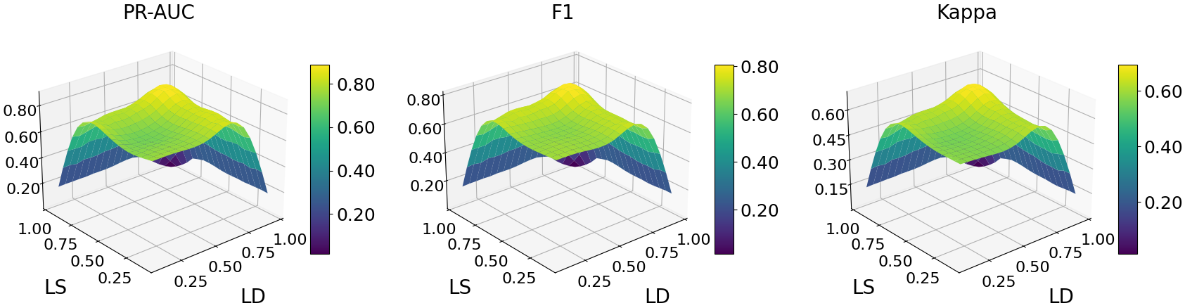
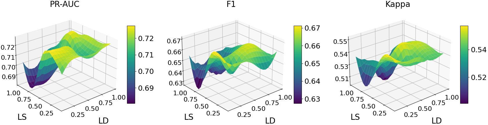
Figure 4: Hyper-parameter study visualization on the Kidney dataset

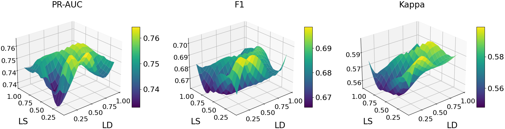
Figure 5: Hyper-parameter study visualization on the COPD dataset

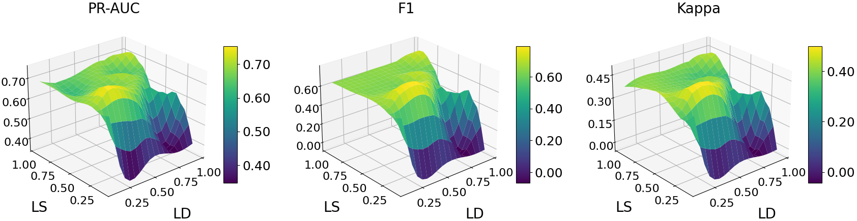
Figure 6: Hyper-parameter study visualization on the Amnesia dataset

Figure 7: Hyper-parameter study visualization on the MIMIC dataset

6.5 Hyperparameter Study

In this section, we explore the effect of hyperparameters on the overall performance of the proposed MedDiffusion. $\lambda_{D}$ controls the magnitude of the diffusion loss, giving the model a restriction on how much deviation is kept in the diffusion; $\lambda_{S}$ controls the relative importance of the generated sequence and punishes the model if the generated sequence does not produce the same prediction as the original prediction. We set up a grid of possible values of $\lambda_{D}=[0.1,0.25,0.5,0.75,1.0]$ and $\lambda_{S}=[0.1,0.25,0.5,0.75,1.0]$, and for each pair, we train our model on the all datasets and record performance in terms of PR-AUC, F1, and Kappa. We visualize the results in the landscape format, as shown in Figure 7, 7, 7, and 7 accordingly.

References

- [1] Yeon S Ahn, Lawrence L Horstman, Wenche Jy, Joaquin J Jimenez, and Brian Bowen. Vascular dementia in patients with immune thrombocytopenic purpura. Thrombosis research, 107(6):337–344, 2002.
- [2] Jacob Austin, Daniel D Johnson, Jonathan Ho, Daniel Tarlow, and Rianne van den Berg. Structured denoising diffusion models in discrete state-spaces. NIPS, 34:17981–17993, 2021.
- [3] Tian Bai, Shanshan Zhang, Brian L Egleston, and Slobodan Vucetic. Interpretable representation learning for healthcare via capturing disease progression through time. In SIGKDD, pages 43–51, 2018.
- [4] Inci M Baytas, Cao Xiao, Xi Zhang, Fei Wang, Anil K Jain, and Jiayu Zhou. Patient subtyping via time-aware lstm networks. In SIGKDD, pages 65–74, 2017.
- [5] Zhengping Che, Yu Cheng, Shuangfei Zhai, Zhaonan Sun, and Yan Liu. Boosting deep learning risk prediction with generative adversarial networks for electronic health records. In ICDM, pages 787–792. IEEE, 2017.
- [6] Chacha Chen, Junjie Liang, Fenglong Ma, Lucas Glass, Jimeng Sun, and Cao Xiao. Unite: Uncertainty-based health risk prediction leveraging multi-sourced data. In WWW, pages 217–226, 2021.
- [7] Yunhao Chen, Yunjie Zhu, Zihui Yan, Jianlu Shen, Zhen Ren, and Yifan Huang. Data augmentation for environmental sound classification using diffusion probabilistic model with top-k selection discriminator. arXiv:2303.15161, 2023.
- [8] Edward Choi, Mohammad Taha Bahadori, Jimeng Sun, Joshua Kulas, Andy Schuetz, and Walter Stewart. Retain: An interpretable predictive model for healthcare using reverse time attention mechanism. NIPS, 29, 2016.
- [9] Edward Choi, Siddharth Biswal, Bradley Malin, Jon Duke, Walter F Stewart, and Jimeng Sun. Generating multi-label discrete patient records using generative adversarial networks. In Machine learning for healthcare conference, pages 286–305. PMLR, 2017.
- [10] Suhan Cui, Junyu Luo, Muchao Ye, Jiaqi Wang, Ting Wang, and Fenglong Ma. Medskim: Denoised health risk prediction via skimming medical claims data. In ICDM, 2022.
- [11] Shansan Gong, Mukai Li, Jiangtao Feng, Zhiyong Wu, and LingPeng Kong. Diffuseq: Sequence to sequence text generation with diffusion models. arXiv:2210.08933, 2022.
- [12] Ian Goodfellow, Jean Pouget-Abadie, Mehdi Mirza, Bing Xu, David Warde-Farley, Sherjil Ozair, Aaron Courville, and Yoshua Bengio. Generative adversarial networks. Communications of the ACM, 63(11):139–144, 2020.
- [13] Jonathan Ho, Ajay Jain, and Pieter Abbeel. Denoising diffusion probabilistic models. NIPS, 33:6840–6851, 2020.
- [14] Sepp Hochreiter and Jürgen Schmidhuber. Long short-term memory. Neural computation, 9(8):1735–1780, 1997.
- [15] Yifan Jiang, Han Chen, and Hanseok Ko. Spatial-temporal transformer-guided diffusion based data augmentation for efficient skeleton-based action recognition. arXiv:2302.13434, 2023.
- [16] Alistair EW Johnson, Tom J Pollard, Lu Shen, Li-wei H Lehman, Mengling Feng, Mohammad Ghassemi, Benjamin Moody, Peter Szolovits, Leo Anthony Celi, and Roger G Mark. Mimic-iii, a freely accessible critical care database. Scientific data, 3(1):1–9, 2016.
- [17] Aki Koivu, Mikko Sairanen, Antti Airola, and Tapio Pahikkala. Synthetic minority oversampling of vital statistics data with generative adversarial networks. JAMIA, 27(11):1667–1674, 2020.
- [18] Akim Kotelnikov, Dmitry Baranchuk, Ivan Rubachev, and Artem Babenko. Tabddpm: Modelling tabular data with diffusion models. In ICML, pages 17564–17579. PMLR, 2023.
- [19] Bum Chul Kwon, Min-Je Choi, Joanne Taery Kim, Edward Choi, Young Bin Kim, Soonwook Kwon, Jimeng Sun, and Jaegul Choo. Retainvis: Visual analytics with interpretable and interactive recurrent neural networks on electronic medical records. IEEE TVCG, 25(1):299–309, 2018.
- [20] Haoying Li, Yifan Yang, Meng Chang, Shiqi Chen, Huajun Feng, Zhihai Xu, Qi Li, and Yueting Chen. Srdiff: Single image super-resolution with diffusion probabilistic models. Neurocomputing, 479:47–59, 2022.
- [21] Xiang Lisa Li, John Thickstun, Ishaan Gulrajani, Percy Liang, and Tatsunori Hashimoto. Diffusion-LM improves controllable text generation. In Alice H. Oh, Alekh Agarwal, Danielle Belgrave, and Kyunghyun Cho, editors, NIPS, 2022.
- [22] Xin-guang Liu, Yu Hou, and Ming Hou. How we treat primary immune thrombocytopenia in adults. Journal of Hematology & Oncology, 16(1):1–20, 2023.
- [23] Junyu Luo, Muchao Ye, Cao Xiao, and Fenglong Ma. Hitanet: Hierarchical time-aware attention networks for risk prediction on electronic health records. In SIGKDD, pages 647–656, 2020.
- [24] Xue-Jing Luo, Shuo Wang, Zongwei Wu, Christos Sakaridis, Yun Cheng, Deng-Ping Fan, and Luc Van Gool. Camdiff: Camouflage image augmentation via diffusion model. arXiv:2304.05469, 2023.
- [25] Fenglong Ma, Radha Chitta, Jing Zhou, Quanzeng You, Tong Sun, and Jing Gao. Dipole: Diagnosis prediction in healthcare via attention-based bidirectional recurrent neural networks. In SIGKDD, pages 1903–1911, 2017.
- [26] Fenglong Ma, Yaqing Wang, Jing Gao, Houping Xiao, and Jing Zhou. Rare disease prediction by generating quality-assured electronic health records. In ICDM, pages 514–522. SIAM, 2020.
- [27] Fenglong Ma, Quanzeng You, Houping Xiao, Radha Chitta, Jing Zhou, and Jing Gao. Kame: Knowledge-based attention model for diagnosis prediction in healthcare. In CIKM, pages 743–752, 2018.
- [28] Liantao Ma, Junyi Gao, Yasha Wang, Chaohe Zhang, Jiangtao Wang, Wenjie Ruan, Wen Tang, Xin Gao, and Xinyu Ma. Adacare: Explainable clinical health status representation learning via scale-adaptive feature extraction and recalibration. In AAAI, volume 34, pages 825–832, 2020.
- [29] Alex Nichol, Prafulla Dhariwal, Aditya Ramesh, Pranav Shyam, Pamela Mishkin, Bob McGrew, Ilya Sutskever, and Mark Chen. Glide: Towards photorealistic image generation and editing with text-guided diffusion models. arXiv:2112.10741, 2021.
- [30] Vadim Popov, Ivan Vovk, Vladimir Gogoryan, Tasnima Sadekova, and Mikhail Kudinov. Grad-tts: A diffusion probabilistic model for text-to-speech. In ICML, pages 8599–8608. PMLR, 2021.
- [31] Aditya Ramesh, Prafulla Dhariwal, Alex Nichol, Casey Chu, and Mark Chen. Hierarchical text-conditional image generation with clip latents. arXiv:2204.06125, 2022.
- [32] Kashif Rasul, Calvin Seward, Ingmar Schuster, and Roland Vollgraf. Autoregressive denoising diffusion models for multivariate probabilistic time series forecasting. In ICML, pages 8857–8868. PMLR, 2021.
- [33] Robin Rombach, Andreas Blattmann, Dominik Lorenz, Patrick Esser, and Björn Ommer. High-resolution image synthesis with latent diffusion models. In CVPR, pages 10684–10695, 2022.
- [34] Chitwan Saharia, Jonathan Ho, William Chan, Tim Salimans, David J Fleet, and Mohammad Norouzi. Image super-resolution via iterative refinement. IEEE TPAMI, 2022.
- [35] Huan Song, Deepta Rajan, Jayaraman Thiagarajan, and Andreas Spanias. Attend and diagnose: Clinical time series analysis using attention models. In AAAI, volume 32, 2018.
- [36] Yusuke Tashiro, Jiaming Song, Yang Song, and Stefano Ermon. Csdi: Conditional score-based diffusion models for probabilistic time series imputation. NIPS, 34:24804–24816, 2021.
- [37] Brandon Trabucco, Kyle Doherty, Max Gurinas, and Ruslan Salakhutdinov. Effective data augmentation with diffusion models. arXiv:2302.07944, 2023.
- [38] Ashish Vaswani, Noam Shazeer, Niki Parmar, Jakob Uszkoreit, Llion Jones, Aidan N Gomez, Łukasz Kaiser, and Illia Polosukhin. Attention is all you need. NIPS, 30, 2017.
- [39] Changrong Xiao, Sean Xin Xu, and Kunpeng Zhang. Multimodal data augmentation for image captioning using diffusion models. arXiv:2305.01855, 2023.
- [40] Fan Yang, Zhongping Yu, Yunfan Liang, Xiaolu Gan, Kaibiao Lin, Quan Zou, and Yifeng Zeng. Grouped correlational generative adversarial networks for discrete electronic health records. In BIBM, pages 906–913. IEEE, 2019.
- [41] Muchao Ye, Suhan Cui, Yaqing Wang, Junyu Luo, Cao Xiao, and Fenglong Ma. Medpath: Augmenting health risk prediction via medical knowledge paths. In WWW, pages 1397–1409, 2021.
- [42] Muchao Ye, Junyu Luo, Cao Xiao, and Fenglong Ma. Lsan: Modeling long-term dependencies and short-term correlations with hierarchical attention for risk prediction. In CIKM, pages 1753–1762, 2020.