In this paper we reconsider the notion of optimality in estimation of partially identified models. We illustrate the general problem in the context of a semiparametric binary choice model with discrete covariates as an example of a model which is partially identified as shown in, e.g. bierenshartog. A set estimator for the regression coefficients in the model can be constructed by implementing the Maximum Score procedure proposed by manski1975. For many designs this procedure converges to the identified set for these parameters, and so in one sense is optimal. But as shown in komarova2013 for other cases the Maximum Score objective function gives an outer region of the identified set. This motivates alternative methods that are optimal in one sense that they converge to the identified region in all designs, and we propose and compare such procedures. One is a Hodges type estimator combining the Maximum Score estimator with existing procedures. A second is a two step estimator using a Maximum Score type objective function in the second step. Lastly we propose a new random set quantile estimator, motivated by definitions introduced in molchanov2006book. Extensions of these ideas for the cross sectional model to static and dynamic discrete panel data models are also provided.

Key Words: Maximum Score, Identified Set, Hodges estimator, Panel Data Discrete Choice.

JEL Codes: C14, C21, C25.

1 Introduction

The binary response model, as well as the more general class of monotone index models have received a great deal of attention in both the theoretical and applied econometrics literature. This is because as many economic variables of interest such as employment status or purchase decisions of a good are of a qualitative nature. The binary choice model is usually represented by some variation of the following equation:

$$y_{i}=I[x_{i}^{\prime}\beta_{0}-\epsilon_{i}\geq 0],$$ (1.1)

where $I[\cdot]$ is the indicator function, $y_{i}$ is the observed response variable taking the values 0 or 1, and $x_{i}$ is an observed vector of covariates which affect the behavior of $y_{i}$. Both the disturbance term $\epsilon_{i}$ and the vector $\beta_{0}$ are unobserved with the latter often being a parameter whose identification is to be characterized and then (point or set) estimated from a random sample of $(y_{i},x_{i}),\quad i=1,2,\ldots.n$.

The disturbance term $\epsilon_{i}$ is restricted in ways that help characterize identification of $\beta_{0}$. Parametric restrictions would specify the distribution of $\epsilon_{i}$ up to a finite number of parameters and would assume it is distributed independently of the covariates $x_{i}$. Under common parametric restrictions, $\beta_{0}$ would be easily established to be point identified as long as the vector $x_{i}$ satisfies the usual rank condition. In these cases $\beta_{0}$ can be consistently point estimated (up to scale) using maximum likelihood or nonlinear least squares. However, except in special cases, these estimators are (point) inconsistent if the distribution of $\epsilon_{i}$ is misspecified or conditionally heteroskedastic. On the other hand, semiparametric or “distribution free” restrictions have also been imposed in the literature, resulting in a variety of identification results and estimation procedures for $\beta_{0}$. One of the first and most influential estimation methods was the “maximum score” estimator proposed in manski1975. In the case of binary choice the conditions in manski1975 for the point identification of $\beta_{0}$ can be shown to be given by the conditional median restriction

$$\mbox{Med}(\epsilon_{i}|x_{i})=0$$ (1.2)

as well as a smoothness and large support condition on the distribution of the index $x_{i}^{\prime}\beta_{0}$. manski1975 proposed the estimator of $\beta_{0}$ which were the set of values maximizing the objective function

$$M_{n}(\beta)=\frac{1}{n}\sum_{i=1}^{n}I[y_{i}=1]I[x_{i}^{\prime}\beta\geq 0]+I[y_{i}=0]I[x_{i}^{\prime}\beta<0]$$ (1.3)

Under stated conditions, manski1975 and manski1985 established (point) identification of $\beta_{0}$ and consistency of the Maximum Score estimator .

In a more general setting, the desirability of an estimator would be driven by its properties when the parameter $\beta_{0}$ is not point identified and, hence, so no point consistent estimator exists. In the model above, point identification can fail for a number of reasons, such as a lack of smoothness or a lack of a large support for $x_{i}^{\prime}\beta_{0}$. One empirically relevant setting is when all the covariates are discretely distributed. This raises the question, which this paper will attempt to address, on how useful the Maximum Score estimation procedure as well as alternative estimation methods can be in this setting. To examine this we will be posing questions such as a) whether a given estimator converges to a set which is meaningful in the sense that it is a strict subset of the parameter space, and b) if that answer is affirmative, how does the set it converges to relate to the identified set? If the two sets (the limiting set of the maximum score estimator, and the identified set) are equal for all designs satisfying the model’s assumptions we will refer to the estimator as sharp. In contrast, if the answer is negative, we will pose the question of the existence of a sharp estimator for the problem at hand, and if the answer is affirmative, propose an estimator and establish its (set) consistency under stated regularity conditions.

The rest of the paper is organized as follows. In Section 2 we consider estimating the binary choice model under a very particular, but illustrative design – one where the disturbance term distribution is not parametrically specified and all the regressors are discretely distributed. It is well known that the regression coefficients in this model are generally not point identified – see, e.g. bierenshartog. The Maximum Score estimator will not be point consistent, so a natural question becomes how it performs as a set estimator. We first establish its asymptotic properties and establish (under stated) conditions that it converges to an outer region of the identified set. This does not imply suboptimality of the Maximum score unless one can construct a procedure that does converge to the identified set.

Section 3 then proposes two new estimation procedures for a semiparametric binary choice model under the median restriction. The first relies on modifying the maximum score objective function by incorporating a data driven switching device. We show it is pointwise optimal in the sense that it converges to the identified set. The second estimator, analogous to that in khan2001, effectively combines the objective functions used in manski1975 and ichimura1994 and is shown to also be optimal pointwise.

Section 4 then introduce the notion of uniform optimality in the sense of estimating the model in question under drifting designs, loosely analogous to that introduced in the unit root and weak iv literatures. The purpose of this is to explore notions of robustness of each of the procedures. Under such drifting designs, Section 5 compares procedures in a more refined fashion by establishing their rates of convergence under both fixed and drifting asymptotics.

Section 6 then extends the concepts, and introduces new procedures for partially identified panel data models, in both static and dynamic settings. Here, the central estimators which we focus discussion on to determine optimality are those proposed in [manski1987] and [honorekyriazidou].

Section 7 concludes by summarizing results and discussing areas for future research.

2 Identification and Estimation of Binary Choice Models

In this section we illustrate our main ideas by introducing the basic concepts of identification and set estimation of the binary choice models we will be working with. This will enable us to formally define our notion of optimality of estimators, including the maximum score estimator, for these models. We will define these basic concepts within the context of the binary choice model

$$y_{i}=I[x_{i}^{\prime}\beta_{0}-\epsilon_{i}\geq 0].$$

Assume a random sample of $n$ observations drawn of the vector $(y_{i},x_{i})$, with $y_{i}$ being an observed binary scalar and $x_{i}$ an observed vector of $K$ covariates. The scalar random variable $\epsilon_{i}$ is unobserved, and the unknown vector $\beta_{0}$ has the same dimension as $x_{i}$ and is to be estimated from the random sample.

Let $B_{I}\subset{\mathbf{R}}^{K}$ be the set of regression coefficients that are consistent with the assumptions of the model, or, the identified set. Let $\widehat{B}\subset{\mathbf{R}}^{K}$ be a set estimator for the target parameter $\beta_{0}$.

We denote both the estimator and the target of estimation as sets as opposed to points in the parameter space. We do it for two reasons. First, estimators such as the maximum score are generally not single valued in finite samples. Furthermore, in discrete models such as the ones we consider, regression coefficients are often not point identified, in the sense that there are multiple values of the regression coefficients that could generate the observed data, even in arbitrarily large samples or in the whole population.

With these basic concepts we can immediately assess the property of an estimator by measuring its distance from the identified set. Following the standard practice in the set estimation literature, we work with the Hausdorff distance. For two sets in $S_{1},S_{2}\subset\mathbf{R}^{K}$, we will denote this distance by $d_{H}(S_{1},S_{2})$. Formally,

$$d_{H}(S_{1},S_{2})\equiv\max\{\sup_{{x\in S_{1}}}\inf_{{y\in S_{2}}}d_{E}(x,y),\,\sup_{{y\in S_{2}}}\inf_{{x\in S_{1}}}d_{E}(x,y)\},$$

where $d_{E}(x,y)$ denotes the Euclidean distance between vectors $x$ and $y$.

The notion of convergence in probability for a set estimator is naturally defined analogously to a point estimator converging in probability to a point in the parameter space.

Definition 1.

A set estimator $\widehat{B}\subset{\mathbf{R}}^{K}$ converges in probability to $B\subset{\mathbf{R}}^{K}$ if $d_{H}(\widehat{B},B)\stackrel{{\scriptstyle p}}{{\rightarrow}}0$.

In this definition $B$ is also a probability limit of $\widehat{B}$ in the definition of convergence in probability in the random set theory (see [molchanov2006book], Definition 6.19). This definition naturally leads to the notion of optimality we will be using throughout this paper.

Definition 2.

Let $B_{I}\subset{\mathbf{R}}^{K}$ be the identified set for a given model, as defined above. We say that estimator $\widehat{B}\subset{\mathbf{R}}^{K}$ is optimal for a given model if $d_{H}(\widehat{B},B_{I})\stackrel{{\scriptstyle p}}{{\rightarrow}}0$.

Remark 1.

Our notion of optimality of an estimator in this paper is only based on its probability limit, and not, say its asymptotic variance, which is the metric often used for optimal point estimation. Despite this limitation, our notion will still be very useful when comparing or ranking competing estimators for parameters in a given model. For example, one set estimator will be preferable to another by our notion if its Hausdorff distance to the identified set converges to a strictly smaller number. This is an analogous to one point estimator being more efficient than another if its asymptotic variance is smaller.

With these definitions in hand we now can return to the binary choice model and explore the relative optimality of the maximum score (MS) estimator, manski1975, focusing on situations where the regression coefficients are not point identified, such as the discrete regressors case alluded to earlier.

2.1 Maximum Score Example Discrete Design

In this section we explore the properties of the MS estimator in a simple design where the regression coefficients are not point identified. Our design is deliberately simple to illustrate the main points in this paper.

We assume a random sample of observations of the bivariate vector $(y_{i},x_{i})$ available to the econometrician and drawn from the model,

$$y_{i}=I[\alpha_{0}+x_{i}-\epsilon_{i}\geq 0],$$ (2.4)

where $y_{i},x_{i}$ are each observed binary random variables. $\alpha_{0}$ is a fixed scalar, unknown to the econometrician and the target of estimation and inference. Further assumptions will be summarized in A1-A3 below. For now, let us make the following additional assumption which is the motivation for using the MS estimator:

$$Med(\epsilon|x)=0\text{ for any }x.$$

Assumption A1 below will additionally imply that $F_{\epsilon|x}$ is strictly increasing everywhere.

In this setting the identified set, which we denote as $\mathcal{A}_{0}$, is the collection of $\alpha$ such that

$$P(Y=1|x)>0.5 \iff\alpha+x>0,$$

$$P(Y=1|x)=0.5 \iff\alpha+x=0.$$

(The second condition uses strict monotonicty of $F_{\epsilon|x}$ around 0.) For this simple design we wish to establish the properties of the MS estimator for $\alpha_{0}$:

$$\widetilde{\cal A}_{ms,n}=\arg\max_{\alpha\in{\cal A}}\frac{1}{n}\sum_{i=1}^{n}y_{i}I[\alpha+x_{i}\geq 0]+(1-y_{i})I[\alpha+x_{i}<0],$$ (2.5)

where ${\cal A}\subset{\mathbf{R}}$ denotes the parameter space.

An alternative way to define the estimator for this discrete design is as in komarova2013. There, the objective function to be optimized is of the form:

$$\widetilde{\cal A}_{ms,n}=\arg\max_{\alpha\in{\cal A}}\sum_{x\in\{0,1\}}(\hat{p}(x)-0.5)\cdot sgn(\alpha+x)\hat{q}(x),$$ (2.6)

where $\hat{p}(x)$ and $\hat{q}(x)$ denote, respectively, a conditional choice probability estimator and the frequency in the sample for a given $x$:

$$\hat{p}(x)=\frac{1}{n\hat{q}(x)}\sum_{j=1}^{n}y_{j}I(x_{j}=x),\quad\hat{q}(x)=1/n\sum_{j=1}^{n}I(x_{j}=x),\quad x\in\{0,1\}.$$ (2.7)

Generally, $\widetilde{\cal A}_{ms,n}$ will be a set of values, as for this design the objective function will not have a unique maximum. The question we are interested in what this set of values converges to as the sample size, denote by $n$, gets arbitrarily large. We will also be interested in the identified set – that is, the set of values of $\alpha_{0}$ that are consistent with the assumptions of the model, and will be the target of any estimator, including the maximum score.

To give a preview of our results, below we establish that the MS estimator is not an optimal estimator in the sense that it does not converge to the identified set in all cases. In fact, whether it does and does not depend on what the value of $\alpha_{0}$ in the data generating process.

Before proceeding with a more technical exposition, we lay out our set of assumptions used to derive formal results.

Assumption A1.

$\epsilon_{i}$ is distributed independently of $x_{i}$, with a positive density on the real line.

Assumption A2.

$\alpha_{0}\in{\cal A}$, a compact subset of the real line.

Assumption A3.

$x_{i}$ has a binary distribution and $P(x_{i}=1)=q\in(0,1)$.

We now look at the identified sets and the performance of the MS estimator for various values of $\alpha_{0}$ in DGP.

2.1.1 Case $\alpha_{0}=0$ (and analogous case $\alpha_{0}=-1$)

Our first theorem begins to characterize the identified set ${\cal A}_{0}$ for the unknown parameter.

Theorem 2.1.

Suppose A1-A3 hold. If $\alpha_{0}=0$, then ${\cal A}_{0}=\{0\}$.

This result is straightforward and its proof is, therefore, omitted.

Thus, in the special case where $\alpha_{0}=0$ in DGP and, hence, the conditional choice probability $P(Y=1|x=0)$ equals 0.5 exactly, the unknown parameter is point identified. This immediately raises two questions: 1) does the MS estimator converge to ${\cal A}_{0}$ in this case, and 2) if it does not converge, is there an estimation procedure that does?

It is helpful for us define the maximum score population set $\widetilde{\cal A}_{ms}$, which is the set of maxima of the limiting maximum score objective function

$$E[y_{i}I[\alpha+x_{i}\geq 0]+(1-y_{i})I[\alpha+x_{i}<0]].$$

As shown in komarova2013, ${\cal A}_{0}$ and ${\cal A}_{ms}$ are not necessarily identical and ${\cal A}_{ms}$ may be a superset of ${\cal A}_{0}$. In particular, this is the case for our simple design, which is shown in Theorem 2.2.

Theorem 2.2.

Under A1-A3, if $\alpha_{0}=0$, then ${\cal A}_{ms}=[-1,\infty)\cap\mathcal{A}$.

Regarding the behavior of the estimator obtained in a sample, we start with an infeasible case when $P(y=1|x)$ are known for $x\in\{0,1\}$. A modified sample maximum score objective function then is the one where the sampling uncertainty only enters through probabilities of various values of $x$:

$$\sum_{x\in\{0,1\}}(P(y=1|x)-0.5)\cdot sgn(\alpha+x).\hat{q}(x)$$ (2.8)

Let $\widehat{\cal A}_{ms,n}$ denote the set of maximizers of (2.8). The theorem below shows that $\widehat{\cal A}_{ms,n}$ is a consistent estimator of ${\cal A}_{ms}$.

Theorem 2.3 (Infeasible MS estimator).

Assume A1-A3, a random sample of $n$ observations of $(y_{i},x_{i})$ and known conditional probabilities of choice. Then $d_{H}(\widehat{\cal A}_{ms,n},{\cal A}_{ms})\stackrel{{\scriptstyle p}}{{\rightarrow}}0$.

Thus, the infeasible MS score estimator $\widehat{\cal A}_{ms,n}$ is not an optimal estimator as it converges to a superset of the identified set.

We now turn to the feasible MS estimator $\widetilde{\cal A}_{ms,n}$. Even in a large sample size $\hat{p}(0)$ will be on either side of $1/2$ with probabilities close to $1/2$. Informally, this will result in the “fluctuations” in the values of the MS estimator. The formal result is in Theorem 2.4

Theorem 2.4 (Feasible MS estimator).

Assume A1-A3 and a random sample of $n$ observations of $(y_{i},x_{i})$. Let $\widetilde{\cal A}_{ms,n}$ be as defined in (2.6). Then

$$\widetilde{A}_{ms,n}=\left\{\begin{array}[]{l}[0,+\infty)\cap\mathcal{A},\quad\text{with prob approaching }1/2,\\ \left[-1,0\right)\cap\mathcal{A},\quad\text{with prob approaching }1/2,\\ \text{other sets},\quad\text{with prob approaching }0.\end{array}\right.$$ (2.9)

This, in particular, implies that $d_{H}(\widetilde{\cal A}_{ms,n},{\cal A}_{ms})\stackrel{{\scriptstyle p}}{{\nrightarrow}}0$ and $d_{H}(\widetilde{\cal A}_{ms,n},{\cal A}_{0})\stackrel{{\scriptstyle p}}{{\nrightarrow}}0$.

The details of what “other sets” may be are given in the proof of this theorem.

Theorem 2.4 shows that $\widetilde{\cal A}_{ms,n}$ is not a consistent estimator of either ${\cal A}_{ms}$ or ${\cal A}_{0}$. Using the random sets theory in molchanov2006book, we can find a weak limit for $\widetilde{A}_{ms,n}$ given in Theorem 2.5.

Theorem 2.5.

Assume A1-A3 and a random sample of $n$ observations of $(y_{i},x_{i})$. Then

$$\widetilde{A}_{ms,n}\stackrel{{\scriptstyle d}}{{\to}}\mathcal{A}_{distr}\equiv t\cdot[0,+\infty)\cap\mathcal{A}+(1-t)\cdot[-1,0)\cap\mathcal{A},$$

where $t$ is a 0/1 binary variable taking both values with equal probability.

To sum up, when $\alpha_{0}=0$, the infeasible MS estimator $\widehat{\cal A}_{ms,n}$ is suboptimal and converges in probability to the superset ${\cal A}_{ms}$ of the identified set. The feasible MS estimator $\widetilde{\cal A}_{ms,n}$ does not have either ${\cal A}_{ms}$ or ${\cal A}_{0}$ as a probability limit. Its asymptotic behavior is best described by a distribution limit which is the random set taking the values $[0,+\infty)$ and $[-1,0)$ with equal probabilities.

While the above result shows a situation where the performance of MS estimators may be considered to be disappointing. it is important to note that this finding is only for one particular value of $\alpha_{0}$ in the parameter space. However, by our definition of optimality even one point suffices to establish suboptimality. Nonetheless, for reasons that will be made clear later in this paper, it will prove useful to consider other values of $\alpha_{0}$ in the parameter space.

For $\alpha_{0}=-1$ the situation is analogous to the case $\alpha_{0}=0$ as we then have ${\cal A}_{0}=\{-1\}$, ${\cal A}_{ms}=(-\infty,0)\cap\mathcal{A}$, $d_{H}(\widehat{\cal A}_{ms,n},{\cal A}_{ms})\stackrel{{\scriptstyle p}}{{\rightarrow}}0$ and $\widetilde{A}_{ms,n}\stackrel{{\scriptstyle d}}{{\to}}t\cdot(-\infty,-1)\cap\mathcal{A}+(1-t)\cdot[-1,0)\cap\mathcal{A},$ where $t$ is a 0/1 binary variable taking both values with equal probability.

2.1.2 Case $\alpha_{0}\notin\{0,-1\}$

It is enough to consider $\alpha_{0}>0$. We have the following result for the identified set:

Theorem 2.6.

Assume A1-A3. If $\alpha_{0}>0$, then ${\cal A}_{0}=(0,+\infty)\cap\mathcal{A}$.

The identified set is no longer a singleton. But our main question still remains – how does the maximum score estimator do? We address this in the same way as we did before.

We start by finding ${\cal A}_{ms}$ – the set of maxima of the limiting maximum score objective function. It is easy to see that ${\cal A}_{ms}=[0,+\infty)\cap\mathcal{A}=\overline{\cal A}_{0}$.

Next, we establish the limit of the sequence of sets attained by the MS estimator from a finite random sample. First, we consider the case of infeasible $\widehat{\cal A}_{ms,n}$ (when conditional choice probabilities are known) and then the feasible $\widetilde{\cal A}_{ms,n}$ when these probabilities have to be estimated from the sample.

For the infeasible case we have

$$\widehat{\cal A}_{ms,n}=\left\{\begin{array}[]{l}[0,+\infty)\cap\mathcal{A},\quad\text{with prob }1-q^{n}\\ \left[-1,+\infty\right)\cap\mathcal{A},\quad\text{with prob }q^{n}\end{array}\right..$$

Given that $0<q<1$, this immediately leads to the following result.

Theorem 2.7.

Assume A1-A3, a random sample of $n$ observations of $(y_{i},x_{i})$ and known conditional choice probabilities. Then $d_{H}(\widehat{\cal A}_{ms,n},{\cal A}_{0})\stackrel{{\scriptstyle p}}{{\rightarrow}}0$.

Of course, we also have that $d_{H}(\widehat{\cal A}_{ms,n},{\cal A}_{ms})\stackrel{{\scriptstyle p}}{{\rightarrow}}0$ as Hausdorff distance remains the same under set closures. To sum up, the infeasible maxim score converges in probability in the Hausdorff distance to the identified set, and is thus optimal in this range of parameter values.

For the feasible MS estimator we have the following result.

Theorem 2.8.

Assume A1-A3 and a random sample of $n$ observations of $(y_{i},x_{i})$. Then

$$\widetilde{A}_{ms,n}=\left\{\begin{array}[]{l}[0,+\infty)\cap\mathcal{A},\quad\text{with prob approaching }1,\\ \text{other sets},\quad\text{with prob approaching }0.\end{array}\right.$$

This implies that $d_{H}(\widetilde{\cal A}_{ms,n},{\cal A}_{0})\stackrel{{\scriptstyle p}}{{\rightarrow}}0$ (as well as $d_{H}(\widetilde{\cal A}_{ms,n},{\cal A}_{ms})\stackrel{{\scriptstyle p}}{{\rightarrow}}0$).

Identical arguments can be used to show optimality of the maximum score estimator for $\alpha_{0}<0$, $\alpha_{0}\neq-1$.

Thus in one sense, maximum score is “nearly” optimal on the parameter space with $\alpha_{0}=0$ and $\alpha_{0}=-1$ being exceptions.

3 Alternative Procedures

Results from the previous section raise the question if there exists an estimation procedure that is optimal in the sense that it converges to the identified set for all values of the parameter in the parameter space. We further explore this here by considering alternative estimation procedures to the maximum score estimator.

3.1 Two Step Closed Form Estimator

Here we consider an alternative procedure for the same binary choice model and compare its optimality properties to the Maximum Score estimator. This estimator relates directly to procedures introduced in ichimura1994 and ahnetal2018. They are based on the following implication of (1.1)-(1.2) (and also strict monotonicity of $F_{\epsilon|x}$ at 0):

$$P(y_{i}=1|x_{i})=\frac{1}{2}\iff x_{i}^{\prime}\beta_{0}=0$$

Based on the above implication, their proposed estimator minimizes

$$\frac{1}{n}\sum_{i=1}^{n}\hat{w}_{i}(x_{i}^{(1)}+x_{i}^{(2)^{\prime}}\theta)^{2}$$

where as a scale normalization, they normalized the first component of $\beta_{0}$ (which is the coefficient on the first regressor $x_{i}^{(1)}$) to focus on estimating remaining components denoted by $\theta_{0}$. In the above equation $\hat{w}_{i}$ is a weighting function estimated in first stage. This weight function assigns more weight to observations where the nonparametrically estimated choice probability is close to $\frac{1}{2}$:

$$\hat{w}_{i}=I\left[\hat{p}_{i}\approx\frac{1}{2}\right],$$

where, in a general framework, $\hat{p}_{i}$ is a first stage nonparametric estimator

$$\hat{p}_{i}=\frac{\sum_{j}y_{j}K_{h}(x_{j}-x_{i})}{\sum_{j}K_{h}(x_{j}-x_{i})}.$$

(in the discrete design we can simply use (2.7)).

We note this procedure is easy to implement, as it is of closed form in each stage. Thus there are no complicated optimization routines needed to construct an estimator, no matter the dimension of $x_{i}$. Under stated conditions ensuring point identification, this estimator was shown to have desirable asymptotic properties, specifically being asymptotically equivalent to maximum score or smoothed maximum score (horowitz-sms). A disadvantage compared to maximum score is that because it involves nonparametric procedures, the choice of kernel function and bandwidth sequence is required. But in this paper we are mostly concerned about its properties when the model is only partially identified as is the case when the regressors are discrete. It is this partial identification setting in which we will explore its optimality properties and compare it to the maximum score.

For expositional convenience, we focus on the simplified model (2.4) under Assumptions A1-A3. We denote the estimator obtained using the idea described above as $\hat{\alpha}_{CF}$.

We begin with the case $\alpha_{0}=0$ for which we know ${\cal A}_{0}=\{0\}$. For this model, we have the following consistency result.

Theorem 3.1.

Suppose conditional choice probabilities are estimated as $\hat{p}_{i}$ in (2.7) (or use kernel function, tuning parameter, $h_{n}\rightarrow 0$, $nh_{n}\rightarrow\infty$ and a weight function $\hat{w}_{i}\equiv I[|\hat{p}_{i}-\frac{1}{2}|\leq\delta_{n}]$ where $\delta_{n}\rightarrow 0$, $n\delta_{n}^{2}\to\infty$). Then when $\alpha_{0}=0$,

$$\hat{\alpha}_{CF}-\alpha_{0}=o_{p}(1)$$

Thus, in our simple discrete setting with $\alpha_{0}=0$ the alternative estimator converges to the identified set, which is a single point. This is in contrast to the MS estimator properties in this setting described above.

Given the favorable performance of this estimator when $\alpha_{0}=0$ (and analogously, when $\alpha_{0}=-1$), we are motivated to explore the performance of this estimator for cases when $\alpha_{0}\notin\{0,-1\}$. Recall it was in this range of parameter values that maximum score was optimal in the sense that it converged to the identified set. Our finding is that the closed form estimator does not converge to the identified set in cases $\alpha_{0}\notin\{0,-1\}$. This is formalized in the next theorem.

Theorem 3.2.

Assume A1-A3 and $\alpha_{0}\notin\{0,-1\}$. Then for any sequence $\delta_{n}$ such that $\delta_{n}\rightarrow 0$, $\hat{\alpha}_{CF}$ may converge to any point in the parameter space. If $\delta_{n}>0$ is bounded away from 0, then $\hat{\alpha}_{CF}$ may converge to a point on boundary of the identified set (or may converge to a point outside it).

Thus, the best possible result we can achieve in these situations is for the closed form estimator to converge to a point on the boundary of the identified set. Otherwise, the limit is not defined or can be defined arbitrarily to be a point anywhere in the parameter space. To sum up, the closed form estimator is suboptimal generically – for most of the possible values $\alpha_{0}$ in the DGP.

So far, we have shown that by our notion of optimality each of the two estimators – Maximum Score (MS) and the closed form (CF) – are suboptimal. Interestingly, their relative performances move in opposite directions of each other depending on how far the true parameter $\alpha_{0}$ is from 0 or $-1$. It is this feature that motivates two additional approaches, discussed in the next two sections, that combine these two estimation procedures. As we will see, to make additional approaches feasible, we will need to relate the value of $\alpha_{0}$ to the choice probability which is nonparametrically identified from the data.

3.2 Objective Function Combination

Here we consider a third procedure which combines features of the first two. Specifically, it uses the same first step nonparametric procedure of the CF estimator, but in the second step optimizes a variant of the maximum score-type objective function after replacing the dependent variable in a modified objective function with the nonparametric estimator of the choice probability. This estimator, denoted by $\widehat{\cal A}_{OFC}$, is defined as.:

$$\widehat{\cal A}_{OFC}=\arg\max_{\alpha\in{\cal A}}\frac{1}{n}\sum_{i=1}^{n}I[\hat{p}_{i}\geq 1/2-\nu_{n}]I[\alpha+x_{i}\geq 0]+I[\hat{p}_{i}\leq 1/2+\nu_{n}]I[\alpha+x_{i}\leq 0]$$ (3.1)

where $\nu_{n}$ is a sequence number converging to 0 with the sample size.

Remark 2.

The above objective function can be viewed as combining features of the objective functions from the previous two estimators. In one sense it is like the MS estimator as it involves inequalities of the index function. But it also relates to the closed form objective function as it contains estimated choice probabilities. Crucially, the inequalities are weak in both directions, giving weight to the observations where the index is equal to zero. It incorporates a “slackness” tuning parameter, $\nu_{n}$ to ensure consistency that is uniform in both point and set identified cases.

The importance of using the slack variable $\nu_{n}$ and non-strict inequalities stems from cases when there is a regressor value $\tilde{x}$ occurring with a positive probability and such that $P(Y=1|\tilde{x})=0.5$. In this case, $\hat{p}_{i}$ for $x_{i}=\tilde{x}$ will fluctuate around 0.5 with a positive probability. In our objective function defining $\widehat{\cal A}_{OFC}$, no matter what side of 0.5 such $\hat{p}_{i}$ is on, as long as it is within $(0.5-\nu_{n},0.5+\nu_{n})$, for large enough sample sizes it is optimal from the optimization perspective to satisfy both inequalities $\alpha+\tilde{x}\geq 0$ and $\alpha+\tilde{x}\leq 0$, hence giving in the limit the identified set $\{-\tilde{x}\}$.

We now formally establish the properties of this estimator. As we did before, we separately consider the cases when $\alpha_{0}\in\{0,-1\}$ (situations related to our comment in the above paragraph) and $\alpha_{0}\notin\{0,-1\}$.

Theorem 3.3.

Under Assumptions A1-A3 and random sampling of the vector $(y_{i},x_{i})$, suppose conditional choice probabilities are estimated as in (2.7) (or using a kernel function and tuning parameter, $h_{n}\rightarrow 0$, $nh_{n}\rightarrow\infty$.)

If $\alpha_{0}\in\{0,-1\}$ and $\nu_{n}\to 0$, $n\nu_{n}^{2}\to\infty$, then $d_{H}(\widehat{\cal A}_{OFC},\alpha_{0})\stackrel{{\scriptstyle p}}{{\rightarrow}}0.$

We next turn attention to the case $\alpha_{0}\notin\{0,-1\}$. Now both conditional choice probabilities are bounded away from 0.5 and, hence, only condition $\nu_{n}\to 0$ is required to guarantee consistency.

Theorem 3.4.

Let $\alpha_{0}\notin\{0,-1\}$ and $\nu_{n}\to 0$. Under A1-A3 and random sampling of the vector $(y_{i},x_{i})$, suppose conditional choice probabilities are estimated as in (2.7) (or using a kernel function and tuning parameter, $h_{n}\rightarrow 0$, $nh_{n}\rightarrow\infty$). Then

$$d_{H}\left(\hat{\cal A}_{OFC},\widetilde{\cal A}_{ms,n}\right)\stackrel{{\scriptstyle p}}{{\rightarrow}}0\quad\text{ and }d_{H}\left(\hat{\cal A}_{OFC},{\cal A}_{0}\right)\stackrel{{\scriptstyle p}}{{\rightarrow}}0.$$

Thus, the estimator obtained by optimization of the combined objective function indeed converges to the identified set for any $\alpha_{0}\in\mathcal{A}$ given a certain choice of the rate of the smoothing sequence.

Our basic point is illustrated in Figures 1 and 2 where we plot the objective functions of the estimators discussed so far as a function of the parameter $\alpha$, for a series of designs which vary on how the true choice probability is from one half (and, thus, driven by what the true $\alpha_{0}$ in DGP is). These graphs hence illustrate which procedures yield set identification and how sharp the bounds are. In the design considered, $x_{i}$ was 0/1 binomial each with probability 0.5, $\epsilon_{i}$ was standard normal, independently of $x_{i}$. The estimators in the graphs are (infeasible) Maximum Score (MS), Closed Form (CF), and Objective Function Combination (OFC). The graphs in Figure 1 are for designs where the parameter is not point identified ($\alpha_{0}=0.5$ is representative of a more general $\alpha_{0}>0$, $\alpha_{0}=-0.5$ is representative of a more general $\alpha_{0}\in(-1,0)$, and $\alpha_{0}=-1.25$ is representative of a more general $\alpha_{0}<-1$). As we see, CF is unhelpful as it cannot even bound the parameter. The other two can, and interestingly, they both yield the same bounds, which we know are sharp from the results in komarova2013.

The graphs in Figure 2 are for designs where the choice probabilities can equal one half. Here CF and OFC yield the sharpest bounds, point identifying the true parameter. MS does not, but they still provide meaningful bounds.

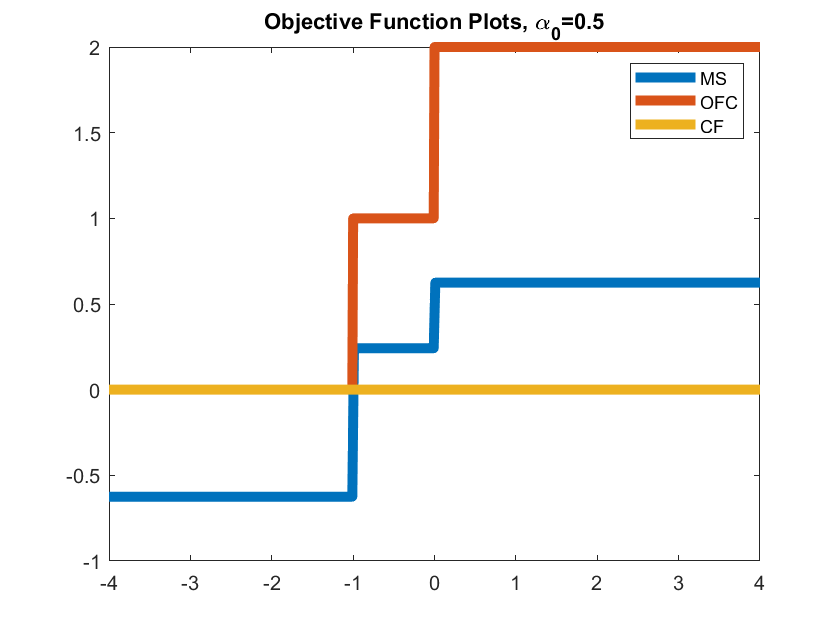
(a) $\alpha_{0}=0.5$ (representative of $\alpha_{0}>0$)

(b) $\alpha_{0}=-0.5$ (representative of $-1<\alpha_{0}<0$)

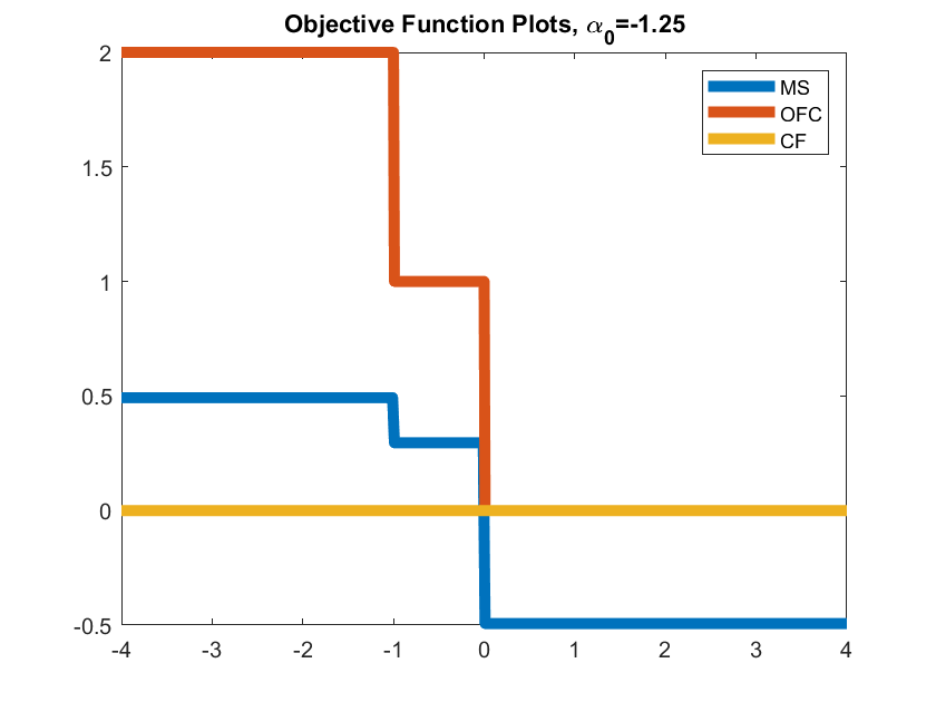
(c) $\alpha_{0}=-1.25$ (representative of $\alpha_{0}<-1$)

Figure 1: Illustration of the objective function values for three estimators for cases $\alpha_{0}\notin\{0,-1\}$.

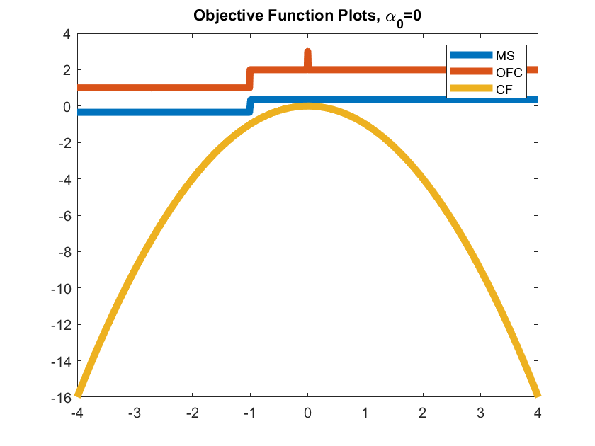
(a) $\alpha_{0}=0$

(b) $\alpha_{0}=-1$

Figure 2: Illustration of the objective function values for three estimators for cases $\alpha_{0}\in\{0,-1\}$.

3.3 “Switching” Estimator

As alluded to towards the end of Section 3, the performances of the MS and CF estimators were inversely related in a certain sense. Heuristically, we found that when one performed well from the convergence in Hausdorff distance perspective, the other did not. This motivates a form of a combination estimator, that can be made feasible with a data driven selection rule.

While for now we describe it in detail only for our illustrative case with the binary regressor and the problem of identifying the intercept, the main idea will apply to the general model, as will its limiting properties.

First, from a random sample of $n$ observations of $(y_{i},x_{i})$ we construct nonparametric estimates $\hat{p}_{i}$ of the conditional choice probabilities at each of the $n$ observations. Second, we define the minimum deviation of estimated choice probabilities from $1/2$: $\hat{P}_{n}^{\ast}=\min_{i=1,\ldots,n}|\hat{p}_{i}-\frac{1}{2}|$.

Our proposed “switching” estimator is

$$\widehat{\cal A}_{H}\equiv\hat{\alpha}_{CF}I[\hat{P}_{n}^{\ast}<\pi_{n}]+\widetilde{\cal A}_{ms,n}I[\hat{P}_{n}^{\ast}\geq\pi_{n}]\quad\text{ for }\pi_{n}\to 0.$$

Thus, our procedure combines the two estimators discussed in the previous sections – naturally, $P_{n}^{\ast}$ being far enough from zero is taken as evidence against having choice probabilities being $1/2$, and $P_{n}^{\ast}$ being close enough from zero is supportive of the opposite case. Naturally, in the former case we can rely on the maximum score estimator and, in the latter case, on the closed form estimator. $\widehat{\cal A}_{H}$ may be a point estimator or a set estimator in finite samples, depending on the data generating process. Theorem 3.5 establishes one of its desirable limiting properties.

Theorem 3.5.

Under Assumptions A1-A3 and random sampling of $(x_{i},y_{i})$, if $\pi_{n}\rightarrow 0$, $n^{2}\pi_{n}\to\infty$ as $n\rightarrow\infty$, then for each possible value of $\alpha_{0}\in{\cal A}$, we have $d_{H}(\widehat{\cal A}_{H},{\cal A}_{0})\stackrel{{\scriptstyle p}}{{\rightarrow}}0.$

Thus we see that the switching estimator is sharp in the sense that for each value of $\alpha_{0}$ in the parameter space, it converges in probability to the identified set. As alluded to previously, we refer to this property as optimal.

3.4 Random Set Quantile Estimator

In this section we outline another approach that can potentially be used as a basis for constructing a consistent estimator of the identified set. It is based on random set theory which has been used in Econometrics since the seminal work in beresteanumolinari2008. Econometric papers, however, for identification analysis and subsequent estimation methodology, have primarily focused on the notion of selection (or, equivalently, Aumann) expectation from that theory and its estimators (also see further work in beresteanumolchanovmolinari2011) and BERESTEANU201217). Here for the models at hand, we work with a completely different notion.

We develop and describe our random set theory based method for our simple case of the discrete regressor design. Following the definition of the $\tau$-th quantile of a random set in molchanov2006book (p.176), in our simple example we propose to use a $1/2+\Delta$ quantile of the closure of $\widetilde{\cal A}_{ms,n}$ as an estimator, where $\Delta\in(0,1/2)$. Note that this notion from molchanov2006book also applies to vector settings.

To motivate this approach, consider the maximum score estimator $\widetilde{\cal A}_{ms,n}$ when $\alpha_{0}=0$. As shown earlier, $\widetilde{\cal A}_{ms,n}$ fluctuates mainly between two sets – $[-1,0)\cap\mathcal{A}$ and $[0,+\infty)\cap\mathcal{A}$ each with a probability strictly less than 1/2 in a sample but approaching 1/2 as $n\to\infty$. In a sample, other finite number of sets are possible with strictly positive probabilities which all approach 0 as $n\to\infty$ (details are in the proof of Theorem 2.4).

That means that if we take the $\tau$’s quantile of the closure $\overline{\widetilde{A}}_{ms,n}$ with $\tau=1/2+\Delta$, $\Delta>0$, then it consists of only $\{0\}$ for large enough $n$ and, thus, converges in probability to the identified set. If, on the other hand, we take the $\tau$’s quantile of $\overline{\widetilde{A}}_{n,ms}$ with $\tau=1/2-\Delta$, $\Delta>0$, then for large enough $n$ it is $[-1,+\infty)\cap\mathcal{A}$ which is an outer region of the identified set and, as discussed above, is the maximand of the population maximum score objective function. With $\tau=1/2$, the quantile of $\overline{\widetilde{A}}_{ms,n}$ for large enough $n$ can be shown to be the two-element set $\{-1,0\}$ and, thus, it does not recover the identified set asymptotically.

Our formal result if given in Theorem 3.6.

Theorem 3.6.

Suppose A1-A3 and random sampling of $(x_{i},y_{i})$. Let $q_{\tau}(\overline{\widetilde{A}}_{ms,n})$ denote the $\tau$-th quantile of random set $\overline{\widetilde{A}}_{n,ms}$, as defined in molchanov2006book (p. 192). If $\tau=1/2+\Delta$, $\Delta\in(0,1/2)$, then

$$d_{H}\left(q_{\tau}(\overline{\widetilde{A}}_{ms,n}),{\cal A}_{0}\right)\stackrel{{\scriptstyle p}}{{\rightarrow}}0.$$

To facilitate a deeper understanding of the concept of random set quantiles, we can draw parallels to voting rules. Let’s begin by examining the median of a random set within the context of our illustrative example.

Imagine an infinite number of random samples $\{(x_{i},y_{i}\}_{i=1}^{n}$ of a fixed size $n$. Each sample casts votes for any number of elements of $\mathcal{A}$ that maximize the maximum score objective function for the given sample. Equivalently, a given sample votes for its respective maximum score estimate $\widetilde{A}_{ms,n}$. After the application of the closure operator $\widetilde{A}_{ms,n}$, majority winners are selected – namely, those elements in $\mathcal{A}$ that are voted for by at least 50% of the samples. The collection of those majority winners would give us $q_{0.5}(\overline{\widetilde{A}}_{ms,n})$. For any arbitrary index $\tau\in(0,1)$, the quantile $q_{\tau}(\overline{\widetilde{A}}_{ms,n})$ comprises those elements from $\mathcal{A}$ that adhere to the ’quota rule’ with a threshold of $\tau$. In simpler terms, these elements within $\mathcal{A}$ must garner votes from at least $100\tau\%$ of the samples to be included.

Feasible version of the random set quantile estimator

The estimator $q_{\tau}(\overline{\widetilde{A}}_{ms,n})$ is infeasible due to the unavailability of $\overline{\widetilde{A}}_{ms,n}$’s distribution within the sample. Central to the issue is our capacity to compute a viable sample quantile for a random set. This challenge assumes heightened complexity within scenarios characterized by the estimations delineated earlier for the case $\alpha_{0}=0$. In such instances, the sample presents not fluctuating variations, but a singular set —- either $(-1,0)$ or $(0,+\infty)$ (other sets can be realized with a decreasingly small probability). Consequently, we are pressed to artificially introduce fluctuations via suitable sampling techniques. Simultaneously, these methods must be engineered in a manner that their impact on cases of $x$ where $P(Y=1|x)\neq 1/2$ remains inconsequential.

In the context of our simple, discrete design, we rely on the interpretation of $\widetilde{\cal A}_{ms,n}$ as the solution set obtained in (2.6). We propose a sampling techniques that will draw $\hat{p}_{s}(x)$, $s=1,\ldots,S$, for each $x\in\{0,1\}$.

Of course, we know that for each $x\in\{0,1\}$,

$$\hat{p}(x)\stackrel{{\scriptstyle a}}{{\sim}}\mathcal{N}\left(p(x),\frac{p(x)(1-p(x))}{n}\right),$$

so it may seem natural to draw $\hat{p}_{s}(x)$ from $\mathcal{N}(\hat{p}(x),\frac{\hat{p}(x)(1-\hat{p}(x))}{n})$. However, if $p(x)=1/2$, then this symmetric way of drawing on both sides of $\hat{p}(x)$ will give an advantage to one of the sets from $(-1,0)$ or $(0,+\infty)$ – if $\hat{p}(x)>1/2$, then the majority of $\hat{p}_{s}(x)$ will be above $1/2$ as well while we need them $\hat{p}_{s}(x)$ to appear in approximately similar proportions on both sides of $1/2$. This leads us to proposing an asymmetric sampling technique.

Namely, if $\hat{p}(x)>1/2$, then

$$\hat{p}_{s}(x)\sim\mathcal{N}\left(\hat{p}(x),\frac{p(x)(1-p(x))}{n}\right)\cdot\mathcal{I}\left(\hat{p}_{s}(x)>\hat{p}(x)\right)+\mathcal{N}\left(\hat{p}(x),\tau\frac{p(x)(1-p(x))}{n}\right)\cdot\mathcal{I}\left(\hat{p}_{s}(x)\leq\hat{p}(x)\right),$$

and if $\hat{p}(x)<1/2$, then

$$\hat{p}_{s}(x)\sim\mathcal{N}\left(\hat{p}(x),\tau\frac{p(x)(1-p(x))}{n}\right)\cdot\mathcal{I}\left(\hat{p}_{s}(x)>\hat{p}(x)\right)+\mathcal{N}\left(\hat{p}(x),\frac{p(x)(1-p(x))}{n}\right)\cdot\mathcal{I}\left(\hat{p}_{s}(x)\leq\hat{p}(x)\right).$$

The value of $\tau>1$ is chosen based on the design/DGP and may depend on the desired quantile index as well as probabilities of $X$ such that $p(x)=0.5$.

Then we consider

$$\widetilde{\cal A}^{\ast}_{ms,n,s}=\arg\max_{\alpha\in{\cal A}}\sum_{x\in\{0,1\}}(\hat{p}_{s}(x)-0.5)\cdot sgn(\alpha+x)\hat{q}(x),\quad s=1,\ldots,S.$$ (3.2)

$q_{\tau}(\overline{\widetilde{A}}_{ms,n})$ ids then estimated by taking a sample $(0.5+\Delta)$-quantile based on the sample of $\{\widetilde{\cal A}^{\ast}_{ms,n,s}\}_{s=1}^{S}$.

Simulation experiment for feasible quantile random set estimator.

Consider $\alpha_{0}=0$ in our simple design. Then $p(0)=1/2$ and $p(1)>\frac{1}{2}$. Let $q_{0}=0.7$ and $\varepsilon\sim\mathcal{N}(0,\sigma^{2})$ with $\sigma=0.5$. We choose sample sizes $n=200$. $n=500$, $n=1000$ and $n=10000$. Figure 3 is representative of the results we get for this case. The illustrations in Figure 3 are for 12 different realizations of $\hat{p}(0)$ in the sample. The blue vertical bars represent probabilities with which $(-1,0)$ (or its closure or a half-closure) is $\widetilde{\cal A}^{\ast}_{ms,n,s}$, and the red vertical bars represent probabilities with which $(0,+\infty)$ (or its closure) is $\widetilde{\cal A}^{\ast}_{ms,n,s}$. Even though for graphical quality we chose to limit our illustration to 12 different realizations of $\hat{p}(0)$, the patterns we see in those graphs are representative of what would happen for other realizations of $\hat{p}(0)$. In particular, we conclude that if we take $\Delta=0.05$, then the $(0.5+\Delta)$th sample quantile of the closure of the maximum score estimand is $\mathcal{A}_{0}=\{\alpha_{0}\}$ with an extremely high probability. Namely, for 1,000 different random sample of size $n=200$ (and, hence, potentially for 1,000 different realizations of $\hat{p}(0)$) only in 2.2% cases the sample $0.55$th quantile obtained in the described above way is a strict superset of $\{0\}$. For 1,000 different random sample of size $n=500$ it is 1.7%. For 1000 different random sample of size $n=1000$ it is 2.2%. For 1,000 different random sample of size $n=10000$ it is 2%. If we slightly increases the quantile index and take $0.5+\Delta=0.6$, then all these percentages for all mentioned $n$ are 0.

In the final comment we note that infrequently $\hat{p}_{s}(x)$ may be drawn outside of their natural $[0,1]$ range,. In this case, one may want to consider

$$\widetilde{\cal A}^{\ast}_{ms,n,s}=\arg\max_{\alpha\in{\cal A}}\sum_{x\in\{0,1\}}(\min\{\max\{0,\hat{p}_{s}(x)\},1\}-0.5)\cdot sgn(\alpha+x)\hat{q}(x),\quad s=1,\ldots,S.$$

instead of (3.2) but this dos not change our conclusions in any way.

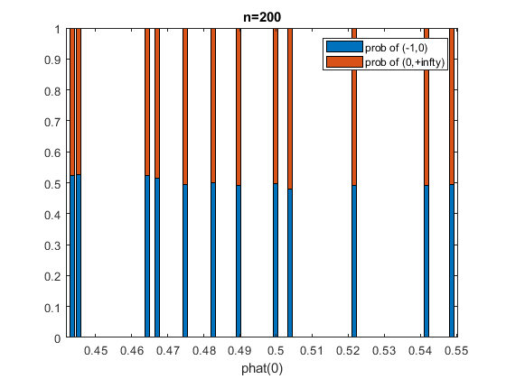
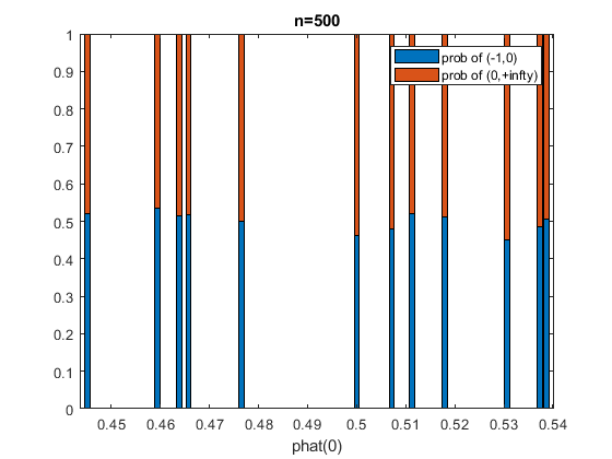
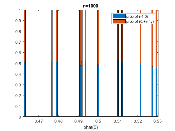
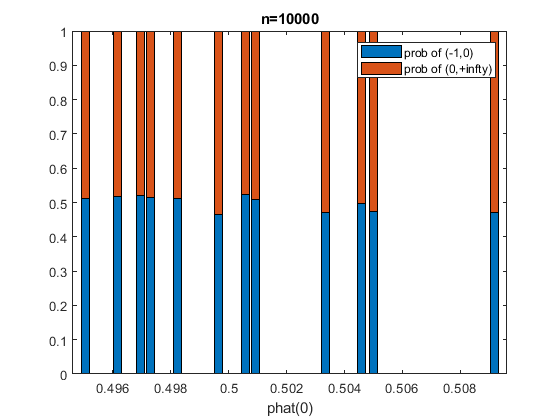
Figure 3: Illustration of the probabilities when $(-1,0)$ or $(0,+\infty)$ delivers the maximum value to the maximum score objective function. These are sample probabilities obtained under sampling $\hat{p}_{s}(x)$, $x\in\{0,1\}$. $s=1,\ldots,2000$.

4 Drifting Parameters in Binary Choice Model

An important additional desirable property of estimators is the local robustness expressed as continuity of their limit with respect to the parameter of interest and nuisance parameters. The example of the Hodges’ estimator when compared to MLE illustrates the role of continuity of the limit of an estimator for choice of the estimator used in practice. We use the same principle to evaluate the estimators we considered previously. We do so in the context of our simple example, with a single binary regressor whose coefficient is normalized to 1 and the parameter of interest being the intercept term.

The structure of the identified set for the parameter of interest $\alpha_{0}$ can be viewed as determined by the probability $p(0)=P(Y=1\,|\,X=0)$ where $p(0)=\frac{1}{2}$ leads to point identification of $\alpha_{0}$ while whenever $p(0)\neq\frac{1}{2}$ the target parameter is partially identified. As a result, we approach the question of robustness of the estimators for the identified by analyzing their limits along the sequences of data generating processes where probability $p^{(n)}(0)$ varies with the sample size $n$ and approaches $\frac{1}{2}$ in the limit.

An important question is the selection of the rate of drifting for the sequence $p^{(n)}(0).$ For the model we consider the focal case where $p(0)=\frac{1}{2}$ and the parameter of interest $\alpha_{0}=0$ is point identified. We then consider the sequence of population distributions indexed by a sequence of probabilities

$$p^{(n)}(0)=\frac{1}{2}+\frac{h}{\sqrt{n}}.$$ (4.1)

and we analyze the limits of our estimators along this sequence of distributions. Because $p^{(n)}(0)=\Phi(\alpha_{n})$, (4.1) automatically implies that

$$\alpha_{n}=\frac{c}{\sqrt{n}}.$$ (4.2)

Consequently, $p^{(n)}(1)$ are drifting too: $p^{(n)}(1)=p(1)+\frac{h_{1}}{\sqrt{n}}$.

We selected this drifting rate by using an alternative interpretation of the maximum score estimator as an ensemble of weak learners (e.g., see section 10.1 in [shalev:14]).

The maximum score objective function can be viewed as an aggregation of “votes” where each observation casts a vote for one of the sets $A^{1}=(-\infty,-1),$ $A^{2}=[-1,0)$ and $A^{3}=[0,+\infty).$ To see this, consider a single element of the maximum score objective function

$$y_{i}\,I[\alpha+x_{i}\geq 0]+(1-y_{i})\,I[\alpha+x_{i}<0].$$

For each possible combination $(y_{i},x_{i})$ the element of the objective function selects the intervals $[-1,+\infty),$ $[0,+\infty),$ $(-\infty,-1)$ and $(-\infty,0).$

We can then interpret this element as a classifier (a “weak learner” in the terminology of the Machine learning literature) which can select one of the sets $A^{1},A^{2}$ and $A^{3}$ or their pairwise unions. For the pairwise union, the classifier selects each set in the union.

Then a classifier corresponding to observation $i$ selects $A^{1}$ and with probability $(1-p(1))q,$ $A^{1}$ and $A^{2}$ with probability $(1-p(0))(1-q),$ $A^{3}$ with probability $p(0)(1-q)$ and $A^{2}$ and $A^{3}$ with probability $p(1)q.$ The machine learning literature calls such a classifier a “weak learner” because the probability that it classifies the object of interest correctly is not diminishing in larger samples. We consider the concept of the weak learner in context of partial identification, novel to the machine learning literature.

Let $v_{i}$ be a three-dimensional vector with elements $1/0$ depending on whether the corresponding set (for each of the three dimensions) was selected by observation $i.$ Then $\bar{v}=\frac{1}{n}\sum^{n}_{i=1}v_{i}$ produces a vector of collective “votes” of $n$ classifiers for each observation $i$ and the maximum score estimator can be written as $\widehat{{\mathcal{A}}}_{ms,n}=A^{\operatorname*{arg\,max}\bar{v}}.$ Note that this interpretation of the maximum score estimator as an aggregator of “votes” is distinct from voting parallels in the discussion of random set quantiles. The key difference is that in case of the random set quantile the “votes” were cast by samples whereas here “votes” are cast by individual observations within a given sample.

The estimator is a function of the sample mean $\bar{v}$ converging at the standard parametric rate $\sqrt{n}$ to a normal random variable. For the analysis of continuity of distribution limit of such parameters the literature (e.g., [ibragimov], [Lecam1953]) suggest considering sequences of the population distributions of the underlying random variable with its expectation drifting at the same parametric rate. Since the expectation of the random vector $v_{i}$ is linear in the probability $p(0),$ sequences of probabilities $p^{(n)}(0)$ drifting at $1/\sqrt{n}$ rate will result in an equivalent drifting of the expectation of $v_{i}$ at that rate.

One could think of other reasons to consider $1/\sqrt{n}$ drifting rate for the parameter. Since the behavior of the estimators we consider is purely driven by the asymptotic behavior of $\hat{p}(0)$ (and in a lesser way by that of $\hat{p}(1)$), we note that the rate of $1/\sqrt{n}$ is the supremum of all the monotonic rates leaving the asymptotic distribution of $\hat{p}(0)$ (and that of $\hat{p}(1)$ unchanged).

4.1 Maximum Score Estimator

We first turn attention to the MS estimator. When $\alpha_{n}$ is the truth, the maxima of the population maximum score objective function is denoted as ${\cal A}_{ms,\alpha_{n}}$, the infeasible maximum score estimator from a sample of size $n$ with known $p(x_{i})$ is denoted as $\widehat{A}_{ms,n,\alpha_{n}}$ and the feasible maximum score estimator with estimated $\hat{p}(x_{i})$ is denoted as $\widetilde{A}_{ms,n,\alpha_{n}}$.

Based on our results in Section 3, it is straightforward to see that under Assumption A1-A3, we have ${\cal A}_{ms,\alpha_{n}}=\overline{\cal A}_{0,\alpha_{n}}=[0,+\infty)$, and

$$\widehat{A}_{ms,n,\alpha_{n}}=\left\{\begin{array}[]{l}\left[0,+\infty\right)\cap\mathcal{A},\quad\text{with prob }1-q^{n},\\ \left[-1,+\infty\right)\cap\mathcal{A},\quad\text{with prob }q^{n}.\end{array}\right.$$

An immediate consequence is that

$$d_{H}\left(\widehat{\cal A}_{ms,n,\alpha_{n}},{\cal A}_{ms,\alpha_{n}}\right)\stackrel{{\scriptstyle p}}{{\rightarrow}}0\quad\text{and}\quad d_{H}\left(\widehat{\cal A}_{ms,n,\alpha_{n}},{\cal A}_{0,\alpha_{n}}\right)\stackrel{{\scriptstyle p}}{{\rightarrow}}0.$$

The performance of the feasible estimator $\widetilde{A}_{ms,n,\alpha_{n}}$ is analyzed in Theorem 4.1.

Theorem 4.1.

Under Assumptions A1-A3, random sampling, and (4.2), we have

$$\widetilde{\cal A}_{ms,n,\alpha_{n}}\stackrel{{\scriptstyle p}}{{\rightarrow}}\mathcal{A}_{distr}(h)\equiv t\cdot[-1,0)+(1-t)\cdot[0,+\infty),$$

where $t$ is a binary random variable taking the value of 0 with probability $\Phi(-\frac{2h}{\sqrt{1-q(1)}})$.

In particular, this implies that

$$\inf_{h\geq 0}\;\text{plim}_{n\to\infty}\;d_{H}\left(\widetilde{\cal A}_{ms,n,\alpha_{n}},{\cal A}_{0,\alpha_{n}}\right)=0,\quad\inf_{h\geq 0}\;\text{plim}_{n\to\infty}\;d_{H}\left(\widetilde{\cal A}_{ms,n,\alpha_{n}},{\cal A}_{ms,\alpha_{n}}\right)=0.$$

One implication of Theorem 4.1 is that parameter drifting in this case can bridge two regimes. One regime is the one where asymptotically the feasible MS estimator fluctuates with equal probabilities between sets $[-1,0)$ and $[0,+\infty)$ (corresponds to $h=0$). This regime describes the behavior of the maximums score estimator without drifting which we earlier established in Theorem 2.3. The second regime is where the maximum score estimator effectively coincides with the set $\overline{\mathcal{A}}_{0,\alpha_{n}}$ with probability 1 (corresponds to $h=+\infty$) which is a desirable case from the perspective of the behavior under drifting.

To summarize, as $h$ varies from $0$ to $+\infty,$ the distribution of the random set varies from equal randomization between $[-1,0)$ and $[0,+\infty)$ to selecting a fixed set $[0,+\infty).$ Thus, this choice of the drifting sequence indeed bridges the two cases.

Based on our results in this section, one can conclude that maximum score satisfies certain uniformity properties. Based on this, we pose the question on whether this type of uniformity should be incorporated in the definition when ranking set estimators, analogous to MLE being optimal in point estimation.

We next explore the properties of both the two-step closed form procedure and combination procedures under drifting parameter sequence.

4.2 Two-step Closed Form procedure

Let $\hat{\alpha}_{CF.n}$ denote the closed form estimator obtained from a sample when $\alpha_{n}$ is the truth. We have the following theorem:

Theorem 4.2.

Assume A1-A3 and (4.1). Let the weight function be $\hat{w}_{i}=I\left[|\hat{p}_{i}-1/2|<\delta_{n}\right]$ with $\delta_{n}\to 0$, $n\delta_{n}^{2}\to\infty$. Then

$$d_{H}(\hat{\alpha}_{CF,n},{\cal A}_{0,\alpha_{n}})\stackrel{{\scriptstyle p}}{{\nrightarrow}}0.$$

(but $\hat{\alpha}_{CF,n}\stackrel{{\scriptstyle p}}{{\rightarrow}}0$.)

4.3 Objective Function Combination Estimator

Let $\hat{\cal A}_{OFC,n}$ denote the estimator defined as in (3.1) with $\alpha_{n}$ as the truth.

Theorem 4.3.

Assume A1-A3 and (4.1). Suppose $\nu_{n}\to 0$, $n\nu_{n}^{2}\to\infty$. Then

$$d_{H}(\hat{\cal A}_{OFC,n},\mathcal{A}_{0,\alpha_{n}})\stackrel{{\scriptstyle p}}{{\nrightarrow}}0$$

(but $d_{H}(\hat{\cal A}_{OFC,n},\{0\})\stackrel{{\scriptstyle p}}{{\rightarrow}}0$. )

Thus, as we can see, the OFC estimator and the identified setdo not get arbitrarily close in probability in terms of the Hausdorff distance.

4.4 Switching Estimator

Let $\widehat{\cal A}_{H,n}$ denote the “switching” estimator with $\alpha_{n}$ as the truth:

$$\widehat{\cal A}_{H,n}=\hat{\alpha}_{CF,n}I[\hat{P}_{n}^{*}<\pi_{n}]+\widetilde{\cal A}_{ms,n}I[\hat{P}_{n}^{*}\geq\pi_{n}].$$

We have the following theorem.

Theorem 4.4.

Assume A1-A3 and (4.1). Suppose $\pi_{n}\to 0$, $n\pi_{n}^{2}\to\infty$. Then

$$d_{H}(\widehat{\cal A}_{H,n},\mathcal{A}_{0,\alpha_{n}})\stackrel{{\scriptstyle p}}{{\nrightarrow}}0$$

(but $d_{H}(\widehat{\cal A}_{H,n},\{0\})\stackrel{{\scriptstyle p}}{{\rightarrow}}0$)

Proofs of this result and others pertaining to the switching estimator under drifting asymptotics can be found in Section I. The main conclusion is that the switching estimator does not get arbitrarily close to $\mathcal{A}_{0,\alpha_{n}}$ under drifting.

Remark 3.

From the perspective of the uniformity properties, the original maximum score estimator has better performance than the other three discussed. The closed form, the OFC and the “switching” estimators have poor uniform properties. Interestingly, the very attributes that enable their effectiveness in specific point-identified cases, such as $\alpha_{0}\in{0,-1}$, are also responsible for their weaker performance in terms of uniformity.

4.5 Random set quantile estimator

Our last result in Section 4 is on the behavior of the quantile of the closure of the MS estimator with the MS estimator being treated as a random set and, hence, with the notion of the quantile applied from the random set theory (see molchanov2006book). Just as in Section 3, for simplicity we focus on the infeasible quantile estimator which under the drifting sequence (4.1) is denoted as $q_{\tau}(\overline{\widetilde{A}}_{ms,n,\alpha_{n}})$, Theorem 4.5 below establishes the asymptotic behavior of the Hausdorff distance between $q_{\tau}(\overline{\widetilde{A}}_{ms,n,\alpha_{n}})$ and ${\cal A}_{0,\alpha_{n}}$.

Theorem 4.5.

Suppose A1-A3 and random sampling of the vector $(y_{i},x_{i})$. Let $\alpha_{0}=0$, Then for any $h$ in (4.1) there exists $\Delta>0$ small enough such that for the quantile index $\tau=\frac{1}{2}+\Delta$ we have: $d_{H}\left(q_{\tau}(\overline{\widetilde{A}}_{ms,n,\alpha_{n}}),{\cal A}_{0,\alpha_{n}}\right)\stackrel{{\scriptstyle p}}{{\rightarrow}}0.$

Thus, we see this estimator has desirable properties under drifting sequences in the sense that it gets arbitrarily close to $\mathcal{A}_{0,\alpha_{n}}$. Recall that it was also optimal without drifting. While this estimator is infeasible, a consistent estimator of this quantile (see our proposed approach earlier3.6) would also have this properties.

5 Rates of Convergence

In this section, for each of the estimators introduced previously, we will establish its rate of convergence under both point and set identification and under fixed and drifting asymptotics. The purpose here is to further refine our comparison of the various procedures, as the previous section only determined if they were consistent or not. To illustrate these main points here we continue to consider the simple design with one binary regressor, only the intercept parameter $\alpha_{0}$ to be estimated, and the disturbance term following a standard normal distribution. Recall that in that setting the the parameter was point identified when it was $0$ or $-1$ and set identified otherwise.

5.1 Maximum Score Estimator

We first consider the limiting distribution theory for the maximum score estimator in our simple design. Under conditions when the parameter is point identified and the maximum score estimator is consistent, [kimpollard] established both the rate of convergence and limiting distribution of the estimator. However, that does not apply here in the simple design. Recall that even when the parameter is point identified, the maxima of the limiting maximum score objective function may be a set. Its limiting distribution theory can be characterized by Theorems 5.1-5.3, with the last one corresponding to local to zero asymptotics.

To analyze point identified cases, it is enough to consider $\alpha_{0}=0$ (case $\alpha_{0}=-1$ is analogous), and to analyze set identified cases it is enough to consider $\alpha_{0}>0$ (cases $\alpha_{0}<0$, $\alpha_{0}\neq-1$ are analogous).

Theorems 5.1 and 5.2 consider the fixed design.

Theorem 5.1.

Let $\alpha_{0}=0$. Under A1-A3, and random sampling of the vector $(y_{i},x_{i})$,

$$n^{p}d_{H}\left(\widehat{\cal A}_{ms,n},{\cal A}_{ms}\right)\stackrel{{\scriptstyle p}}{{\rightarrow}}0\text{ for any }p>0$$

but

$$d_{H}\left(\widehat{\cal A}_{ms,n},{\cal A}_{0}\right)\stackrel{{\scriptstyle p}}{{\nrightarrow}}0.$$

Thus, in the point identified case $\alpha_{0}$, the infeasible $\widehat{\cal A}_{ms,n}$ converges at an arbitrary fast rate to the maxima of the limiting maximum score objective function, which is ${\cal A}_{ms}=[-1,+\infty)\cap\mathcal{A}$ and is an outer set of the identified set. An analogous result does not apply to the feasible maximum score estimator $\widetilde{\cal A}_{ms,n}$ since, as shown before, it does not converge in Hausdorff distance in probability either to ${\cal A}_{ms}$ or ${\cal{A}}_{0}$.

Theorem 5.2.

Let $\alpha_{0}>0$. Under A1-A3, and random sampling of the vector $(y_{i},x_{i})$,

$$n^{p}d_{H}\left(\widehat{\cal A}_{ms,n},{\cal A}_{0}\right)\stackrel{{\scriptstyle p}}{{\rightarrow}}0,\quad n^{p}d_{H}\left(\widetilde{\cal A}_{ms,n},{\cal A}_{0}\right)\stackrel{{\scriptstyle p}}{{\rightarrow}}0$$

for any $p>0$.

Thus, in set identified cases both $\widehat{\cal A}_{ms,n}$ and $\widetilde{\cal A}_{ms,n}$ converge to ${\cal A}_{0}$ at an arbitrarily fast rate.

Finally, we consider what happens under the drifting sequence. The previous section focused on the case when $\alpha_{0}=0$ and the drifting sequence $\alpha_{n}$ satisfies (4.2). More generally, for any $\alpha_{0}$ we can consider $\alpha_{n}$ such that

$$\alpha_{n}-\alpha_{0}=\frac{c}{\sqrt{n}},\quad c>0.$$ (5.1)

Theorem 5.3 establishes the rate of convergence of $d_{H}(\widetilde{A}_{ms.n,\alpha_{n}},{\cal A}_{0,\alpha_{n}})$ for $\alpha_{0}>0$.

Theorem 5.3.

Let $\alpha_{0}>0$ and $\alpha_{n}$ satisfies (5.1). Under A1-A3, and random sampling of the vector $(y_{i},x_{i})$, for any $p>0$, we have

$$n^{p}d_{H}\left(\widetilde{\cal A}_{ms,n,\alpha_{n}},{\cal A}_{0,\alpha_{n}}\right)\stackrel{{\scriptstyle p}}{{\rightarrow}}0.$$

In this section instead of $n^{p}$, we can take any function of $n$ that grows to $\infty$ with $n$.

5.2 Closed Form Estimator

For the limiting distribution of the closed form estimator, we note the first step properties are particularly easy to determine in the discrete design, as regressors can simply be put into cells so there are no bandwidth conditions to consider. Recall this estimator had an “all or nothing” property pertaining to if we had point identification or not. This feature is also reflected in the limiting distribution theory, as demonstrated in Theorems 5.4-5.5, the latter of which is for drifting asymptotics.

Theorem 5.4 established that in the case of point identification the closed form estimator converges to the identified set arbitrarily fast.

Theorem 5.4.

Suppose A1-A3, and random sampling of the vector $(y_{i},x_{i})$. If $\alpha_{0}=0$ (or $\alpha_{0}=-1$) and $\delta_{n}\to 0$, $n\delta_{n}^{2}\to\infty$, we have for any $p>0$,

$${n}^{p}(\hat{\alpha}_{CF}-\alpha_{0})\stackrel{{\scriptstyle p}}{{\rightarrow}}0.$$

When $\alpha_{0}\notin\{0,-1\}$, then $d_{H}(\hat{\alpha}_{CF},{\cal A}_{0})$ diverges, as established in Theorem 3.2 so there are no additional results for this case.

Finally, Theorem 5.5 considers the drifting asymptotics. It shows that for any drifting sequence (5.1), the closed form estimator $\hat{\alpha}_{CF,n}$ constructed for $\alpha_{n}$ as the truth, does not get close to the identified set ${\cal{A}}_{0,\alpha_{n}}$.

The case of $\alpha_{0}=0$ was considered in Theorem 4.2 (case $\alpha_{0}=-1$ is analogous). Theorem 5.5 considers any $\alpha_{0}$. Even though, for $\alpha_{0}\in\{0,-1\}$ there are smoothing sequences $\delta_{n}$ under which $n^{p}(\hat{\alpha}_{CF,n}-\alpha_{0})\stackrel{{\scriptstyle p}}{{\rightarrow}}0$, an analogous result does not hold for $\alpha_{0}\notin\{0,-1\}$.

Theorem 5.5.

Suppose A1-A3, and random sampling of the vector $(y_{i},x_{i})$. Let the drifting sequence $\alpha_{n}$ satisfy (5.1). Let $\delta_{n}\to 0$, $n\delta_{n}^{2}\to\infty$.

Let $\alpha_{0}\notin\{0,-1\}$. Then

$$d_{H}(\hat{\alpha}_{CF,n},{\cal A}_{0,\alpha_{n}})\stackrel{{\scriptstyle p}}{{\nrightarrow}}0,\quad\hat{\alpha}_{CF,n}-\alpha_{0}\stackrel{{\scriptstyle p}}{{\nrightarrow}}0.$$

Let $\alpha_{0}\in\{0,-1\}$. Then for any $p>0$,

$$d_{H}(\hat{\alpha}_{CF,n},{\cal A}_{0,\alpha_{n}})\stackrel{{\scriptstyle p}}{{\nrightarrow}}0,\quad n^{p}(\hat{\alpha}_{CF,n}-{\alpha}_{0})\stackrel{{\scriptstyle p}}{{\rightarrow}}0.$$

Thus, Theorem 5.5 confirms that the closed form estimator has poor uniformity properties and is never close to ${\cal A}_{0,\alpha_{n}}$ under drifting.

5.3 Objective Function Combination Estimator

In Theorem 5.6 we consider the case of no drifting and establish the arbitrary rate of convergence to the identified set ${\cal A}_{0}$ for feasible $\widehat{\cal{A}}_{OFC}$.

Theorem 5.6.

Suppose A1-A3, and random sampling of the vector $(y_{i},x_{i})$. For any $\alpha_{0}$, for any $p>0$, if $\nu_{n}\to 0$ and $n\nu_{n}^{2}\to\infty$, then

$$n^{p}d_{H}(\widehat{\cal A}_{OFC},{\cal{A}}_{0})\stackrel{{\scriptstyle p}}{{\rightarrow}}0.$$

Theorem 5.7 considers the drifting design.

Theorem 5.7.

Suppose A1-A3, and random sampling of the vector $(y_{i},x_{i})$. Let $\nu_{n}\to 0$, $n\nu_{n}^{2}\to\infty$, Let $\alpha_{n}$ satisfy (5.1).

If $\alpha_{0}\notin\{0,-1\}$, then for any $p>0$, $n^{p}d_{H}(\widehat{\cal A}_{OFC,n},{\cal{A}}_{0,\alpha_{n}})\stackrel{{\scriptstyle p}}{{\rightarrow}}0$.

If $\alpha_{0}\in\{0,-1\}$, then $d_{H}(\widehat{\cal A}_{OFC,n},{\cal{A}}_{0,\alpha_{n}})\stackrel{{\scriptstyle p}}{{\nrightarrow}}0$.

The result of Theorem 5.7 establish the arbitrary rate of convergence to the identified set ${\cal A}_{0,\alpha_{n}}$ obtained treating $\alpha_{n}$ when parameters are drifting to the parameter resulting in a set identified case. However, as established earlier in Theorem 4.3, sets $\widehat{\cal A}_{OFC,n}$ and ${\cal{A}}_{0,\alpha_{n}}$ do not get close to each other in Hausdorff distance when parameters are drifting to the value corresponding to the point identified case.

5.4 “Switching” estimator

Our first result in Theorem 5.8 is for the case of no drifting. Theorem 5.9 shows the performance of the “switching” estimator $\hat{\cal A}_{H,n}$ obtained when $\alpha_{n}$ is the truth.

Theorem 5.8.

Suppose A1-A3 and a random sampling of $(y_{i},x_{i})$. Suppose $\pi_{n}\to 0$, $n\pi_{n}^{2}\to\infty$ and $\delta_{n}\to 0$, $n\delta_{n}^{2}\to\infty$. Then for any $\alpha_{0}\in{\cal A}$ and any $p>0$,

$$n^{p}d_{H}(\hat{\cal A}_{H},{\cal A}_{0})\stackrel{{\scriptstyle p}}{{\rightarrow}}0.$$

In the case of drifting, we already considered the case $\alpha_{0}=0$ in Section 4 in Theorem 4.4. Theorem 5.9 considers other cases of drifting as well.

Theorem 5.9.

Let $\alpha_{n}$ satisfy (5.1). Suppose A1-A3 and a random sampling of $(y_{i},x_{i})$. Also let $\pi_{n}\to 0$, $n\pi_{n}^{2}\to\infty$ and $\delta_{n}\to 0$, $n\delta_{n}^{2}\to\infty$.

If $\alpha_{0}\notin\{0,-1\}$, for any $p>0$,

$$n^{p}d_{H}(\hat{\cal A}_{H,n},{\cal A}_{0,\alpha_{n}})\stackrel{{\scriptstyle p}}{{\rightarrow}}0.$$

If $\alpha_{0}\in\{0,-1\}$, then

$$d_{H}(\hat{\cal A}_{H,n},{\cal A}_{0,\alpha_{n}})\stackrel{{\scriptstyle p}}{{\nrightarrow}}0.$$

5.5 Random set quantile estimator

We first consider teh fixed design and establish that the random set quantile estimator $q_{\tau}(\overline{\cal A}_{ms,n})$, $\tau\in(\frac{1}{2},1)$, (for simplicity, we focus on this infeasible estimator) converges to ${\cal A}_{0}$ arbitrarily fast.

Theorem 5.10.

Suppose A1-A3 and random sampling of $(y_{i},x_{i})$. Then for any $\alpha_{0}$, for any $p>0$,

$$n^{p}d_{H}(q_{\tau}(\overline{\widetilde{A}}_{ms,n}),{\cal A}_{0}){\rightarrow}0.$$

Next, Theorem 5.11 establishes the properties of $q_{\tau}(\overline{\widetilde{A}}_{ms,n,\alpha_{n}})$ under drifting. Even though it considers the case when the drifting sequence satisfies (5.1) (to make it possible to compare to results from other estimators), its result will hold under any rate of the drifting sequence as along as it converges to $\alpha_{0}$.

Theorem 5.11.

Suppose A1-A3 and random sampling of $(y_{i},x_{i})$. Let $\alpha_{n}$ satisfy (5.1).

If $\alpha_{0}=0$ , then for any $h>0$, there exists a quantile index $1/2+\Delta$ close enough to $1/2$ such that for any $p>0$,

$$n^{p}d_{H}(q_{\tau}(\overline{\widetilde{A}}_{ms,n,\alpha_{n}}),{\cal A}_{0,\alpha_{n}}){\rightarrow}0.$$

Case $\alpha_{0}=-1$ is analogous.

If $\alpha_{0}\notin\{0,-1\}$, for any $p>0$,

$$n^{p}d_{H}(q_{\tau}(\overline{\widetilde{A}}_{ms,n,\alpha_{n}}),{\cal A}_{0,\alpha_{n}}){\rightarrow}0$$

for any $\tau=1/2+\Delta$, $\Delta>0$.

6 A Ranking of the estimators

After conducting a comprehensive analysis of the estimators under the influence of drift, we are now able to propose a ranking system based on their uniformity properties.

Our findings reveal that among the estimators considered —- namely, OFC, “switching”, and quantile random sets estimators – each exhibits sharp pointwise characteristics. Conversely, both the Ichimura and Maximum Score estimators lack this pointwise sharpness, and interestingly, they demonstrate poor performance in diametrically opposite scenarios.

Regarding the uniformity properties, we can rank the quantile random set estimator as most robust because for any constant $h$ in the drifting rate (4.1) we can find a range of quantile indices for which it has good uniformity properties. We can rank Maximum Score as second best because one can get arbitrarily close to good uniform properties by selecting a very large drifting constant $h$ in (4.1).

OFC and “switching” estimators are next in the ranking as they have similarly inferior uniformity properties. It is hard to craete a rank between themselves as in their pointwise behavior they have same robustness properties to mistakes made in the rates of the nuisance parameter sequences.

To clarify this point further, the OFC estimator remains informative even when $\nu_{n}\to 0$ fails the condition $n\nu_{n}^{2}\to\infty$. Suppose e.g. that $n\nu_{n}^{2}\to 0$. Then in our focal cases $\alpha_{0}\in\{0,-1\}$ the OFC estimator will behave exactly like the feasible maximum score estimator fluctuating with equal probabilities between two sets. Suppose e.g. that $n\nu_{n}^{2}\to\text{positive finite constant }c_{0}$. Then in our focal cases $\alpha_{0}\in\{0,-1\}$ the OFC estimator will behave by fluctuating among three sets – $\{\alpha_{0}\}$ and the two sets from the asymptotic maximum score behaviors. The limiting probabilities in these fluctuations will be determine by $c_{0}$. The choice of increasingly large $c_{0}$ will result in the probability assigned to $\{\alpha_{0}\}$ in the fluctuations to be increasingly close to 1. The choice of increasingly small $c_{0}$ will result in the probability assigned to $\{\alpha_{0}\}$ in the fluctuations to be increasingly close to 0 and the estimator essentially becoming the feasible maximum score estimator.

Similarly, the “switching estimator” retains its informativeness even when the choice of $\pi_{n}\to 0$ violates the condition $n\pi_{n}^{2}\to\infty$. Should $n\pi_{n}^{2}$ approach zero, the “switching” estimator becomes the feasible maximum score estimator. Conversely, if $n\pi_{n}^{2}$ tends towards a positive finite constant designated as $c_{H}$, and $\alpha_{0}\in{0,-1}$, the “switching” estimator fluctuates among three sets: ${\alpha_{0}}$ and the two sets characteristic of asymptotic feasible maximum score behavior. The probabilities assigned to these fluctuations are determined by the value of $c_{H}$, with larger values of $c_{H}$ driving the probability assigned to ${\alpha_{0}}$ closer to 1, while smaller values of $c_{H}$ result in this probability approaching 0, essentially transforming the estimator into the feasible maximum score estimator in the latter case.

Lastly, we note the Ichimura (closed form) estimator occupies the lowest position in our ranking due to its complete lack of informativeness when all choice probabilities deviate from $1/2$, even by an arbitrarily small amount.

7 Binary Panel Data Model

In this section we consider the identification of a binary choice model with fixed effects. anderson70 considered the problem of inference on fixed effects models from binary response panel data. He showed that inference is possible if the disturbances for each panel member are known to be white noise with the logistic distribution and if the observed explanatory variables vary over time. Nothing need be known about the distribution of the fixed effects and he proved that a conditional maximum likelihood estimator consistently estimates the model parameters up to scale. Interestingly, recent work demonstrates how crucial the logistic distribution assumption is for point identification and consistent estimation. chamberlain2010 shows that when the observable covariates have bounded support, the logistic assumption on an unobserved component is necessary for point identification.

manski1987 showed that identification of the regression coefficients remains possible if the disturbances for each panel member are known only to be time-stationary with unbounded support and if the observed explanatory variables vary enough over time and have large support.

Specifically, he considered the model:

$$y_{it}=I[\alpha_{i}+x_{it}^{\prime}\beta_{0}+\epsilon_{it}>0]$$ (7.1)

where $i=1,2,...n,t=1,2$. The binary variable $y_{it}$ and the $K$-dimensional regressor vector $x_{it}$ are each observed and the parameter of interest is the $K$ dimensional vector $\beta_{0}$. The unobservables are $\alpha_{i}$, and $\epsilon_{it}$, the former not varying with $t$ and often referred to as the “fixed effect” or the individual specific effect. manski1987 imposes no restrictions on the conditional distribution of $\alpha_{i}$ conditional on $x_{i}\equiv x_{i1},x_{i2}$. manski1987 proposed the conditional maximum score estimator to estimate $\beta_{0}$ up to scale. He defined this estimator as the maximizer of the objective function

$$\arg\min\frac{1}{n}\sum_{i=1}^{n}I[y_{i2}\neq y_{i1}]|(y_{i2}-y_{i1})-I[(x_{i2}-x_{i1})^{\prime}\beta>0]|$$ (7.2)

In establishing its asymptotic properties, manski1987 imposed the following conditions:

1. $F_{\epsilon_{i1}|x_{i},\alpha_{i}}(\cdot|\cdot)=F_{\epsilon_{i2}|x_{i},\alpha_{i}}(\cdot|\cdot)$ for all $\alpha_{i},x_{i}$.

2. The support of $\epsilon_{it}|x_{i},\alpha_{i}$ is $R$.

3. Let $w_{i}=x_{i2}-x_{i1}$. Then the support of $w_{i}$ does not lie in proper linear subspace of $R^{K}$.

4. There exists at least one $k\in\{1,2,...K\}$ such that $\beta_{k}\neq 0$ and $w_{i}^{(k)}$, the $k^{th}$ component of $w_{i}$, is distributed continuously with support on the real line conditional on the other components of $w_{i}$.

5. The sample $(y_{i}\equiv(y_{i1},y_{i2}),x_{i})$    $i=1,2,...N$ is i.i.d.

We note the 4th condition will be violated if all the regressors are discrete. This prompts an inquiry into the properties of the conditional maximum score estimator within this particular context. Notably, as we will show, in certain scenarios this estimator tends to converge towards an outer region of the identified set.

Let $\mathcal{X}\in\mathbf{R}^{2k}$ represent the support of $x=(x_{1},x_{2})$, characterized by a finite set of points. To provide further clarity on the observed lack of sharpness,we reframe the population maximum score objective function as follows:

$$\max_{b}\frac{1}{n}\sum_{x=(x_{1},x_{2})\in\mathcal{X}}sgn((x_{2}-x_{1})^{\prime}b)\left(P(y_{2}=1|x)-P(y_{1}=1|x)\right)$$

This formulation mirrors the work of Manski (1987). However, it is essential to acknowledge that the cases where $P(y_{2}=1|x)=P(y_{1}=1|x)$, which play a vital role in pinpointing the parameter of interest in the formal identification approach

$$P(y_{2}=1|x)=P(y_{1}=1|x)\quad\Leftrightarrow\quad(x_{2}-x_{1})^{\prime}\beta=0,$$

are omitted from the population maximum score objective function. Consequently, this leads to the issue of the sharpness of the maximum score estimation approach.

To follow up on our remark, let us consider an illustrative design in this panel data case.

Static panel illustrative design. Let $k=2$ and let $x_{it}$, $t=1,2$, have the support of $\mathcal{X}=\{-1,1\}\times\{-1,1\}$, and $x_{i}=(x_{i1},x_{i2})$ have the support $\mathcal{X}\times\mathcal{X}$. Let $(\varepsilon_{i1},\varepsilon_{i2})$ be independent of $(\alpha_{i},x_{i})$. Take $\beta=(\beta_{1},\beta_{2})^{\prime}=(1,1)^{\prime}$. Then

$$P(y_{i2}=1|x_{i1}=(1,-1)^{\prime},x_{i2}=(-1,1)^{\prime}) =P(y_{i1}=1|x_{i1}=(1,-1)^{\prime},x_{i2}=(-1,1)^{\prime})\quad\text{Case A}$$

$$P(y_{i2}=1|x_{i1}=(-1,1)^{\prime},x_{i2}=(1,-1)^{\prime}) =P(y_{i1}=1|x_{i1}=(-1,1)^{\prime},x_{i2}=(1,-1)^{\prime})\quad\text{Case B}$$

are the equalities that drive the identification of $\beta$ (we would have the same equalities if we additionally conditioned on $\alpha_{i}$) as they imply that

$$\beta_{1}-\beta_{2}=0$$

where $\beta_{1},\beta_{2}$ denote the first and second components of $\beta$, and, together with the normalization restriction $\beta_{1}=1$ will imply that $\beta_{2}=1$, thus indicating that the identified set (in $\beta_{2}$) is $\{1\}$.

The population maximum score objective function will have zero entry corresponding to $x_{i}$ in Cases A and B above. It will have non-zero entries only for the following cases: (i) $x_{it}=(1,1)$, $x_{i,-t}=(-1,-1)$, (ii) $x_{it}=(1,1)$, $x_{i,-t}=(1,-1)$, (iii) $x_{it}=(1,1)$, $x_{i,-t}=(-1,1)$, (iv) $x_{it}=(-1,-1)$, $x_{i,-t}=(1,-1)$, (v) $x_{it}=(-1,-1)$, $x_{i,-t}=(-1,1)$. This objective function will thus be maximized at $\beta$ that satisfy the following inequalities:

$$\beta_{1}>0,\quad\beta_{2}>0,\quad\beta_{1}+\beta_{2}>0.$$

with the normalization $\beta_{1}=1$ we get the following argmax (in $b_{2}$) of this objective function: $(0,+\infty)$ which is a superset of the identification set $\{1\}$. This, once again, illustrates a lack of sharpness in the infeasible/population maximum score estimation. $\blacksquare$

As was the case in the cross sectional case, one can also consider a two- step closed form estimator for the panel data model that is analogous to ichimura1994. To see how, construct the random variable

$$d_{i12}=I[y_{i2}>y_{i1}]$$

for $i=1,2,...N$, and define $d_{i21}$ analogously. Let $p_{i12}$ denote $E[d_{i12}|x_{i}]$ and define $p_{i21}$ analogously. Identification and estimation of $\beta_{0}$ up to scale would be based on

$$I[p_{i12}=p_{i21}]\iff\Delta x_{i}^{\prime}\beta=0$$ (7.3)

where $\Delta x_{i}$ denotes $x_{i2}-x_{i1}$. To construct an estimator based on 7.3, let $\hat{p}_{i12},\hat{p}_{i21}$ denote kernel regression estimators of $p_{i12},p_{i21}$. From these kernel weights could be constructed as

$$\hat{\omega}_{i}=k_{h}(\hat{p}_{i12}-\hat{p}_{i21})$$

where $k(\cdot)$ is a kernel function, $k_{h}(\cdot)=k(\frac{\cdot}{h})$ and $h$ is a bandwidth. With these weights one could estimate $\theta_{0}$, the last $K-1$ components of $\beta_{0}$ by weighted least squares of the first component of $\Delta x_{i},$ denoted by $\Delta x_{i}^{(1)}$ on the remaining $K-1$ components, denoted by $-\Delta x_{i}^{(2)}$.

With these estimators defined one can proceed to easily define estimators analogous to those defined in previous sections of this papers. For example one can define a combination (Hodges) estimator, an objective function combination estimator, and a median random set estimator, all in the panel data setting.

We are able to show analogous results for the panel data setting as those we found in the cross sectional setting. Specifically, using identical arguments, we are able to show:

1. Neither the conditional maximum score nor the closed form estimator estimators are sharp, though the conditional maximum score estimator is robust.

2. The combination (Hodges) estimator is sharp but not robust compared to the conditional Maximum Score estimator.

3. An analogously defined combination objective function and median random set estimators are both sharp but only the latter is robust.

Formal statements of these results and their proofs are delegated to the appendix, Section G.

7.1 Dynamic Binary Panel Data Model

Here we consider the binary dynamic panel data model that relates the outcome in period $t$ for individual $i$, $y_{it}$, to its lagged value $y_{i,t-1}$ in the following way

$$y_{it}=I[x_{it}^{\prime}\beta+\gamma y_{i,t-1}+\alpha_{i}+\epsilon_{it}\geq 0]\ \ t=1,2,...T$$ (7.4)

Here we are interested in learning about $\theta=(\gamma,\beta^{\prime})^{\prime}$. This $\theta$ is treated as a fixed (but unknown) constant vector while the unobservables here take the standard form $\epsilon_{it}+\alpha_{i}$ where $\alpha_{i}$ is an individual specific and time independent “fixed effect,” and is meant to capture the systematic correlation of the unobservables over time while $\epsilon_{it}$ is an idiosyncratic error term that is both time and entity specific. The parameter $\gamma$ is of special interest as it measures the effect of state dependence.

In econometric theory, the literature that has studied this model is vast the theoretical results we will focus on here are in honorekyriazidou, who proposed an estimator based on a conditional maximum score objective function.

They assumed the the binary dependent variable is observed for 4 time periods ($t=0,1,2,3$) and the regressors are observed for 3 periods ($t=1,2,3$). They defined their estimator as $\hat{\theta}\equiv(\hat{\gamma},\hat{\beta})$, the maximizer with respect to $\theta$ of the objective function:

$$\frac{1}{n}\sum_{i=1}^{n}K\left(\frac{x_{i23}}{h_{n}}\right)\hbar_{i}(\theta)$$ (7.5)

where $K(\cdot)$ denotes a kernel function and $h_{n}$ denotes a bandwidth sequence whose properties are detailed below, and $\hbar_{i}(\theta)\equiv y_{i21}\cdot\operatorname*{sign}(z_{i}^{\prime}\theta)$. Where, following their notation, variables with double subscripts denote time differences: e.g, $x_{i23}\equiv x_{i2}-x_{i3}$, and $z_{i}\equiv(x_{i12},y_{i03})$.

To establish the (point) consistency of this estimator they imposed the following conditions

1. $\epsilon_{it}$ is distributed independently of $x_{i}$ and independently across time with a cdf $F(\cdot)$ that is strictly increasing on the real line for all $(x_{i},\alpha_{i})$

2. There exists a component of $\beta$, denoted by $\beta^{(\kappa)}$ s.t. $\beta^{(\kappa)}\neq 0$, and the corresponding component of $x_{21i}$ is continuously distributed with positive density on the real line, conditional on the remaining components of $x_{21i}$ and conditional on $x_{23i}$ lying in a neighborhood of 0.

3. The support of $x_{12i}$ conditional on $x_{23i}$ in a neighborhood of zero is not contained in any proper linear subspace of ${\mathbf{R}}^{k}$

4. The random vector $x_{23i}$ is absolutely continuously distributed with density $f(\cdot)$ that is bounded from above on its support and strictly positive in a neighborhood of zero.

5. For all $\theta\in\Theta$, $E[h(\theta)|x_{23i}=\cdot]$ is continuously differentiable on its support with bounded first order derivatives.

6. The kernel function $K:{\mathbf{R}}^{k}:\rightarrow{\mathbf{R}}$ is a function of bounded variation that is bounded from above and below and integrates to 1.

7. The bandwidth sequence $h_{n}$ is a sequence of positive numbers that satisfies $h_{n}\rightarrow 0$ and $nh_{n}^{k}/\log n\rightarrow\infty$

We note here two crucial conditions for their point identification results. One is continuity of one of the regressors in each of the time periods. This is not surprising as it was required for the static binary panel data model as well. The other is an overlap support condition- specifically they assume that each component of $x_{i2}$ has support that overlaps with the corresponding component of $x_{i3}$. To relate our results in this section to those found in previous sections of this paper we will maintain the overlap support condition in honorekyriazidou, but assume $x_{i}$ has discrete support. Consequently, we will assume that $P(x_{i2}=x_{i3})>0$ and redefine the objective function as

$$\frac{1}{n}\sum_{i=1}^{n}I[x_{i23}=0]\hbar_{i}(\theta)$$ (7.6)

In this dynamic panel data case we can present a illustrative design in the spirit of illustrative designs earlier to establish lack of sharpness of honorekyriazidou estimator when we consider the case of discrete regressors.

Dynamic panel illustrative design. Let $k=2$ and let $x_{it}$ have the support $\mathcal{X}=\{0,1\}^{2}$, and let $x_{i}=(x_{i1},x_{i2},x_{i3})$ have the support $\mathcal{X}^{3}$. Let $\varepsilon_{I}=(\varepsilon_{i1},\varepsilon_{i2},\varepsilon_{i3})$ be independent of $(\alpha_{i},x_{i})$. Let $\varepsilon_{it}$ be independent across time and have strictly increasing c.d.f.. Take $\beta=(\beta_{1},\beta_{2})^{\prime}=(-1,1)^{\prime}$ and $\gamma=-1$. Suppose the distribution of the initial $y_{i0}$ is independent of $(x_{i},\alpha_{i},\varepsilon_{i})$.

Denote

$$A(d_{0},d_{3}) =\{y_{i0}=d_{0},y_{i1}=0,y_{i2}=1,y_{i3}=d_{3}\},$$

$$B(d_{0},d_{3}) =\{y_{i0}=d_{0},y_{i1}=1,y_{i2}=0,y_{i3}=d_{3}\}$$

Then

$$P(A(0,1)|\alpha_{i},x_{i},x_{i2}=x_{i3})\\ =(1-F_{\varepsilon}(x_{i1}^{\prime}\beta+\alpha_{i}))F_{\varepsilon}(x_{i2}^{\prime}\beta+\alpha_{i})F_{\varepsilon}(x_{i3}^{\prime}\beta-1+\alpha_{i})F(y_{i0}=0)$$

$$P(B(0,1)|\alpha_{i},x_{i},x_{i2}=x_{i3})\\ =F_{\varepsilon}(x_{i1}^{\prime}\beta+\alpha_{i}))(1-F_{\varepsilon}(x_{i2}^{\prime}\beta-1+\alpha_{i}))F_{\varepsilon}(x_{i3}^{\prime}\beta+\alpha_{i})F(y_{i0}=0)$$

Take $x_{i1}=(0,0)$ and $x_{i2}=x_{i3}=(0,1)$. Then

$$x_{i1}^{\prime}\beta=0,\quad x_{i2}^{\prime}\beta=1,\quad x_{i3}^{\prime}\beta=1$$

and, clearly,

$$P(A(0,1)|\alpha_{i},x_{i1}=(0,0),x_{i2}=x_{i3}=(0,1))=P(B(0,1)|\alpha_{i},x_{i1}=(0,0),x_{i2}=x_{i3}=(0,1)).$$

This implies immediately the following identifiability restriction $(x_{i2}-x_{i1})^{\prime}b+g(y_{i3}-y_{i0})=0$ which takes the form

$$b_{2}+g=0.$$ (7.7)

Analogously,

$$P(A(0,1)|\alpha_{i},x_{i1}=(1,1),x_{i2}=x_{i3}=(0,1))=P(B(0,1)|\alpha_{i},x_{i1}=(1,1),x_{i2}=x_{i3}=(0,1)).$$

This implies the following identifiability restriction

$$-b_{1}+g=0.$$ (7.8)

Together with the normalization $b_{2}=1$, restrictions (7.7) and (7.8) are enough to conclude that the identified set is a singleton $\{((1,-1)^{\prime},-1)\}$.

The population Honore-Kyriazidou objective function will have zero entry corresponding to cases

$$P(A(d_{0},d_{3})|\alpha_{i},x_{i},x_{i2}=x_{i3})=P(B(d_{0},d_{3})|\alpha_{i},x_{i},x_{i2}=x_{i3}).$$

This is because in these cases

$$P(y_{i2}-y_{i1}=1|\alpha_{i},x_{i},x_{i2}=x_{i3},y_{i0}=d_{0},y_{i3}=d_{3})=P(y_{i2}-y_{i1}=-1|\alpha_{i},x_{i},x_{i2}=x_{i3},y_{i0}=d_{0},y_{i3}=d_{3}),$$

thus resulting in

$$E[y_{i2}-y_{i1}|x_{i},x_{i2}=x_{i3},y_{i0}=d_{0},y_{i3}=d_{3}]=0.$$

This is analogous to what was happening in the maximum score estimation in the illustrative design there – cases driving point identification of the parameter of interest were ignored by the population maximum score objective function.

Let us now construct the set of $(b,g)$ that will maximize the population Honore-Kyriazidou objective function in our design.

Suppose, for example, that $\alpha_{i}$ is also 0/1 variable. Then we have the following system of inequalities defining the maxmimzer of the population Honore-Kyriazidou objective function:

$$b_{1}+b_{2}+g <0,\quad b_{1}-b_{2}+g<0,\quad b_{1}-b_{2}-g<0,\quad-b_{1}-b_{2}+g<0.$$

This set is a subset of $(-\infty,0)\times(0,+\infty)\times(-\infty,0)$. With the normalization $b_{2}=1$ we obtain

$$b_{1}+g <-1,\quad b_{1}+g<1,\quad b_{1}-g<1,\quad-b_{1}+g<1.$$

Removing redundant inequalities it is

$$b_{1}+g <-1,\quad b_{1}-g<1,\quad-b_{1}+g<1.$$

The solution set to these inequalities can be described as

$$\left\{\lambda\cdot(b_{1},g)^{\prime}:\,b_{1}=t,g=-t-1,\;\;t\in[-1,0],\quad\lambda\geq 1\right\}.$$

This set includes $\beta_{1}=-1$ and $\gamma=-1$ as an interior point (take $t=-1/2$ and $\lambda=2$ in the description of the set). Thus, the maximizer of the population Honore-Kyriazidou objective function is a (unbounded) superset of the identified set. This maximizer is displayed in Figure 4.

Figure 4: Maximizer of the population Honore-Kyriazidou objective function in the dynamic panel data illustrative design

If we look at the maximizer of the sample Honore-Kyriazidou objective function, then analogously to the cross sectional case, this maximizer will fluctuate among a finite number of disjoint sets with probabilities bounded away from zero and one. Each of such sets will have the truth $\beta_{1}=-1$ and $\gamma=-1$ at the boundary and the union of all such sets will give the described above maximizer of the population objective function (again, analogous to our illustrative example in the cross sectional case). We can once again show that the random set quantile of the feasible estimator for quantile indices strictly above $1/2$ will give the truth $\beta_{1}=-1$ and $\gamma=-1$ for large enough sample sizes. $\blacksquare$

We can show analogous results for the dynamic panel data setting to those found in the static panel and cross sectional setting. Specifically,

1. The dynamic conditional maximum score is not sharp nor is a closed form analogous estimator, though the dynamic conditional maximum score estimator is robust.

2. An analogous combination (Hodges) estimator is sharp but not robust compared to the weighted conditional Maximum Score estimator for the dynamic model that was proposed in honorekyriazidou.

3. An analogous dynamic combination objective function and a dynamic median random set estimator are both sharp but only the latter is robust.

Formal statements of these results and their proofs are delegated to the appendix.

8 Conclusions

In this paper we further explored the notion of optimal estimation of regression coefficients in binary choice models. Here our notion of optimality pertains to, but is a refined notion of estimating the sharp set. As pointed out in komarova2013, who establishes the form of the identified set for the binary choice model introduced in manski1975, the maximum score estimator introduced in that paper converges to an outer region of the identified set and is hence suboptimal. We propose several novel estimators which are optimal by that notion. Two are combination estimators- the first employs a data driven switching method to adaptively choose between the maximum score estimator and a closed form estimator introduced in ichimura1994. The second combines the objective functions employed in the two estimators, as opposed to the estimators themselves. We prove that each procedure converges to the identified set. A third estimator we propose is referred to as a random set quantile (RSQ) estimator which we show is also optimal. Then similar ideas are used to study binary choice panel data models. Here we propose new estimators that converge to the identified sets in both static and dynamic models, in contrast to existing procedures often used in the literature.

Our work here leaves open areas for future research. There are several nonlinear models of wide interest from both theoretical and empirical perspectives which suffer from the same identification issues as the ones studied in this paper. One example is the class of discrete response models under independence restrictions, which we elaborate on in the Appendix in Section E. But there are many more which need to be explored, such as ordered, multinomial response and simultaneous discrete response models. Procedures based on maximum score or rank regression which have analogous suboptimal properties have been proposed in mjleeordered, kotmultinomial, abrevhaus. We aim to show in future work that our procedures introduced here can result in optimal estimation for those models as well.

Appendix A Appendix

A.1 Proofs in Section 2

Proof of Theorem 2.2. In our special design limiting maximum score objective function can be rewritten as

$$\sum_{x\in\{0,1\}}(P(y=1|x)-0.5)\cdot sgn(\alpha+x)q(x),$$

where $q(x)=P(x_{i}=x)$. Since $P(y=1|x=0)=0.5$ and $P(y=1|x=0)>0.5$, only the case $x=1$ effectively enters the objective function. ${\cal A}_{ms}$ is then given as the set of $\alpha$ that solve $\alpha+1\geq 0$. $\blacksquare$

Proof of Theorem 2.3. $\widehat{\cal A}_{ms,n}$ can be descried as

$$\widehat{\cal A}_{ms,n}=\left\{\begin{array}[]{l}[-1,+\infty)\cap\mathcal{A},\quad\text{with prob }1-(1-q)^{n},\\ \mathcal{A},\quad\text{with prob }(1-q)^{n},\end{array}\right.$$

with the former case being the situation when there are realizations of $x=1$ in the sample, and the latter case being the situation when only $x=0$ values are available in the sample. The fact that $0<q<1$ immediately gives that $P\left(\widehat{\cal A}_{ms,n}\neq{\cal A}_{ms}\right)\to 0$. This implies the result for the Hausdorff distance as $P(d_{H}(\widehat{\cal A}_{ms,n}\neq{\cal A}_{ms})>\epsilon_{0})\leq P\left(\widehat{\cal A}_{ms,n}\neq{\cal A}_{ms}\right)$ for any $\epsilon_{0}>0$. $\blacksquare$

Proof of Theorem 2.4. We obtain $[0,+\infty)\cap\mathcal{A}$ as $\widetilde{\cal A}_{ms,n}$ when $\hat{p}(1)>0.5$ and $\hat{p}(0)>0.5$. Set $\left[-1,0\right)\cap\mathcal{A}$ is obtained as $\widetilde{\cal A}_{ms,n}$ when $\hat{p}(1)>0.5$ and $\hat{p}_{0}<0.5$. Both of these situations happen with probabilities approaching 0.5 as $n\rightarrow\infty$. Indeed,

$$Pr\left(\hat{p}_{1}>0.5,\hat{p}_{0}>0.5\right)=\\ \sum_{k=1}^{n-1}P\left(\sum_{i=1}^{n}y_{i}1(x_{i}=1)>0.5(n-k),\;\sum_{i=1}^{n}y_{i}1(x_{i}=0)>0.5k\;|\;\sum_{i=1}^{n}1(x_{i}=0)=k\right){{n}\choose{k}}q^{n-k}(1-q)^{k}=\\ \sum_{k=1}^{n-1}\left(\sum_{m_{1}=[\frac{n-k}{2}]+1}^{n-k}{{n-k}\choose{m_{1}}}p_{1}^{m_{1}}(1-p_{1})^{n-k-m_{1}}\right)\times\left(\sum_{m_{0}=[\frac{k}{2}]+1}^{k}{{k}\choose{m_{0}}}(1/2)^{k}\right)\times{{n}\choose{k}}q^{n-k}(1-q)^{k}=\\ =\frac{1}{2}\sum_{-+k=1}^{n-1}\left(\sum_{m_{1}=[\frac{n-k}{2}]+1}^{n-k}{{n-k}\choose{m_{1}}}p_{1}^{m_{1}}(1-p_{1})^{n-k-m_{1}}\right)\times\left(1-\frac{{{k}\choose{\frac{k}{2}}}}{2^{k}}\cdot 1(k-even)\right)\times{{n}\choose{k}}q^{n-k}(1-q)^{k},$$

where $p_{c}=P(Y=1|x=c)$, $c\in\{0,1\}$. Since $P\left(\hat{p}_{1}>0.5,\hat{p}_{0}<0.5\right)$ is the same as $P\left(\hat{p}_{1}>0.5\hat{p}_{0}>0.5\right)$, and $P\left(\hat{p}_{1}>0.5\right)\to 1$, and it is easy to establish that $P\left(\hat{p}_{1}>0.5,\hat{p}_{0}=0.5\right)\to 0$ as $n\rightarrow\infty$, we can conclude

$$P\left(\hat{p}_{1}>0.5,\hat{p}_{0}<0.5\right)=P\left(\hat{p}_{1}>0.5,\hat{p}_{0}>0.5\right)\to 0.5.$$

Other sets possible as realization of $\widetilde{\cal A}_{ms,n}$ are $[-1,+\infty)\cap\mathcal{A}$ (when $\hat{p}_{1}>0.5,\hat{p}_{0}=0.5$), or $[0,+\infty)\cap\mathcal{A}$ (when $\hat{p}_{1}=0.5,\hat{p}_{0}>0.5$), or $(-\infty,0)\cap\mathcal{A}$ (when $\hat{p}_{1}=0.5,\hat{p}_{0}<0.5$), or $\mathcal{A}$ (when $\hat{p}_{1}=0.5,\hat{p}_{0}=0.5$), or $(-\infty,-1)\cap\mathcal{A}$ (when $\hat{p}_{1}<0.5,\hat{p}_{0}\leq 0.5$). When $\hat{p}_{1}<0.5,\hat{p}_{0}>0.5$, then either $[0,+\infty)\cap\mathcal{A}$ or $(-\infty,-1)\cap\mathcal{A}$ can be the minimand. All these situations, however, occur with the probability approaching 0 as $n\to\infty$.

For any $0<\epsilon_{0}<1$, $P\left(d_{H}(\widetilde{\cal A}_{ms,n},{\cal A}_{ms})>\epsilon_{0}\right)\to 0.5$ as $n\rightarrow\infty.$ $\blacksquare$

Proof of Theorem 2.5. As follows from Theorem 6.5 in molchanov2006book, it is enough for us to establish in terms of the capacity functional $T$ that for any compact $K\subset\mathbf{R}$,

$$T_{\widetilde{A}_{ms,n}}(K)\to T_{\mathcal{A}_{distr}}(K).$$

Take $K$ such that $K\subset(-\infty,-1)$. Then $T_{\mathcal{A}_{distr}}(K)=0$ and $T_{\widetilde{A}_{ms,n}}(K)\leq Pr\left(\hat{p}_{1}<0.5\right)=\to 0.$

Take $K$ such that $K\subset[-1,0)$. Then $T_{\mathcal{A}_{distr}}(K)=0.5$ and $T_{\widetilde{A}_{ms,n}}(K)=Pr\left(\hat{p}_{1}>0.5,\hat{p}_{0}\leq 0.5\right)+Pr\left(\hat{p}_{1}=0.5,\hat{P}_{0}=0.5\right)=\to 0.5.$

Take $K$ such that $K\subset[0,+\infty)$. Then $T_{\mathcal{A}_{distr}}(K)=0.5$ and $|T_{\widetilde{A}_{ms,n}}(K)-0.5|\leq|Pr\left(\hat{p}_{1}>0.5,\hat{p}_{0}\geq 0.5\right)-0.5|+Pr(\hat{p}_{1}=0.5,\hat{p}_{0}\geq 0.5)+Pr(\hat{p}_{1}<0.5,\hat{p}_{0}>0.5)\to 0$.

Situations when $K$ belongs to pairwise unions of the sets $(-\infty,-1)$, $[-1,0)$, $[0,+\infty)$ or spans across all three these sets are considered analogously. $\blacksquare$

Proof of Theorem 2.6. Since both $p_{0},p_{1}>1/2$, the identified set is characterized by inequalities $\alpha+0>0$ and $\alpha+1>0$ thus giving $(0,+\infty)\cap\mathcal{A}$. $\blacksquare$

Appendix B Proofs in Section 3

Proof of Theorem 3.1. For $x_{i}=1$, $P(\hat{w}_{i}=1)\to 0$, and for $x_{i}=0$, $P(\hat{w}_{i}=0)\to 1$. Hence, with probability approaching 1, $\hat{\alpha}_{CF}+0=0,$ or equivalently, $P(\hat{\alpha}_{CF}\neq 0)\to 0$. $\blacksquare$

Proof of Theorem 3.3. It is enough to consider $\alpha_{0}=0$ as the case $\alpha_{0}=-1$ is analogous. Let

$$S_{nF}(\alpha)=\frac{1}{n}\sum_{i=1}^{n}I[\hat{p}_{i}\geq\frac{1}{2}-\nu_{n}]I[\alpha+x_{i}\geq 0]+I[\hat{p}_{i}\leq\frac{1}{2}+\nu_{n}]I[\alpha+x_{i}\leq 0],$$

$$n_{0}=\sum I[x_{i}=0].$$

Then

$$S_{nF}(\alpha)=\left\{\begin{array}[]{l}\frac{n_{0}}{n}\left(I[\hat{p}(0)\geq\frac{1}{2}-\nu_{n}]+I[\hat{p}(0)\leq\frac{1}{2}+\nu_{n}]\right)+\left(1-\frac{n_{0}}{n}\right)I[\hat{p}(1)\geq\frac{1}{2}-\nu_{n}],\quad\alpha=0,\\ \frac{n_{0}}{n}I[\hat{p}(0)\geq\frac{1}{2}-\nu_{n}]+\left(1-\frac{n_{0}}{n}\right)I[\hat{p}(1)\geq\frac{1}{2}-\nu_{n}],\quad\alpha>0,\\ \frac{n_{0}}{n}I[\hat{p}(0)\leq\frac{1}{2}+\nu_{n}]+\left(1-\frac{n_{0}}{n}\right)I[\hat{p}(1)\geq\frac{1}{2}-\nu_{n}],\quad\alpha\in(-1,0),\\ \frac{n_{0}}{n}I[\hat{p}(0)\leq\frac{1}{2}+\nu_{n}]+\left(1-\frac{n_{0}}{n}\right)\left(I[\hat{p}(1)\leq\frac{1}{2}+\nu_{n}]+I[\hat{p}(1)\geq\frac{1}{2}-\nu_{n}]\right),\quad\alpha=-1\\ \frac{n_{0}}{n}I[\hat{p}(0)\leq\frac{1}{2}+\nu_{n}]+\left(1-\frac{n_{0}}{n}\right)I[\hat{p}(1)\leq\frac{1}{2}+\nu_{n}],\quad\alpha<-1\end{array}\right.$$

Therefore,

$$P(\hat{\alpha}_{OFC}=0) \geq P\left(\hat{p}(0)\in\left[\frac{1}{2}-\nu_{n},\frac{1}{2}+\nu_{n}\right],\;\hat{p}(1)>\frac{1}{2}+\nu_{n}\right)$$

$$\geq P\left(\hat{p}(0)\in\left[\frac{1}{2}-\nu_{n},\frac{1}{2}+\nu_{n}\right]\right)-P\left(\hat{p}(1)\leq\frac{1}{2}+\nu_{n}\right)$$

$$=1-P\left(|\hat{p}(0)-\frac{1}{2}|>\nu_{n}\right)-P\left(\hat{p}(1)\leq\frac{1}{2}+\nu_{n}\right).$$

Since $\hat{p}(0)$ converges to $\frac{1}{2}$ and $\hat{p}(1)$ converges to $p_{1}>1/2$ at the parametric rate with limiting normal distributions, then as $n\to\infty$, for some $c_{0},c_{1}>0$

$$P(|\hat{p}(0)-\frac{1}{2}|>\nu_{n})=P(\sqrt{n}|\hat{p}(0)-\frac{1}{2}|>\sqrt{n}\nu_{n})\leq c_{0}\cdot e^{-n\nu_{n}^{2}}\to 0,$$

$$P(\hat{p}(1)\leq\frac{1}{2}+\nu_{n})=P(\sqrt{n}(\hat{p}(1)-p(1))\leq\sqrt{n}(\underbrace{\frac{1}{2}-p(1)+\nu_{n}}_{<0\text{ for large }n})\leq c_{1}\cdot e^{-n(\frac{1}{2}-p(1)+\nu_{n})^{2}}\to 0.$$

The exponential bounds follow from the tail behavior of the normal distribution.$\blacksquare$

Proof of Theorem 3.4. Taking into account that $p(0)>\frac{1}{2}$, $p(1)>\frac{1}{2}$ for $\alpha_{0}>0$, note that for large enough $n$,

$$S_{nINF}(\alpha)=\frac{\sum I(x_{i}=0)}{n}I[\alpha\geq 0]+\frac{\sum I(x_{i}=1)}{n}I[\alpha\geq 1].$$

Its maximand $\hat{\cal A}_{OFCINF}$ coincides with $\widehat{\cal A}_{ms,n}$.

The feasible estimator $\hat{\cal A}_{OFC}$ has the following property:

$$\hat{\cal A}_{OFC}=\left\{\begin{array}[]{l}\overline{{\cal A}_{0}}={\cal A}_{ms},\quad\text{with prob approaching }1,\\ \text{other sets},\quad\text{with prob approaching }0.\end{array}\right.$$

Other sets are $[-1,0)\cap\mathcal{A}$ and also all the “other sets” listed in the proof of Theorem 2.4.

This establishes our result since we have that

$$d_{H}\left(\hat{\cal A}_{OFC},{{\cal A}_{0}}\right)\stackrel{{\scriptstyle p}}{{\rightarrow}}0,\quad d_{H}\left(\hat{\cal A}_{OFCINF},{\cal A}_{0}\right)\stackrel{{\scriptstyle p}}{{\rightarrow}}0.$$

Earlier in the paper we also established that $d_{H}(\widetilde{\cal A}_{ms,n},{\cal A}_{0})\stackrel{{\scriptstyle p}}{{\rightarrow}}0$, which together with results obtained here implies that $d_{H}\left(\hat{\cal A}_{OFCINF},\widetilde{\cal A}_{ms,n}\right)\stackrel{{\scriptstyle p}}{{\rightarrow}}0$. $\blacksquare$

Proof of Theorem 3.5. We demonstrate our result for the simple discrete design used throughout Section 3.

For illustration purposes, we first consider the infeasible case where the choice probabilities are known. For this case, we use notation $P_{n}^{\ast}$ instead of $\hat{P}_{n}^{\ast}$. Starting with the case $\alpha_{0}=0$, we have

$$|p(x_{i})-{1}/{2}|=0\cdot I[x_{i}=0]+(\underbrace{p(1)-{1}/{2}}_{\equiv\delta>0})\cdot I[x_{i}=1].$$

Hence, with a random sample of $n$ observations, $P_{n}^{\ast}$ is a random variable which, when $\alpha_{0}=0$, takes the value 0 with probability $1-q^{n}$ and takes a strictly positive value with probability $q^{n}$. For any $\epsilon_{0}>0$ we then have

$$P(d_{H}(\widehat{\cal A}_{H},\{0\})>\epsilon_{0}) = P(d_{H}(\widehat{\cal A}_{H},\{0\})>\epsilon_{0},P_{n}^{\ast}<\pi_{n})+P(d_{H}(\widehat{\cal A}_{H},\{0\})>\epsilon_{0},P_{n}^{\ast}\geq\pi_{n})$$

$$= P(|\hat{\alpha}_{CF}-0|>\epsilon_{0},P_{n}^{\ast}<\pi_{n})+P(d_{H}(\widehat{\cal A}_{H},\{0\})>\epsilon_{0},P_{n}^{\ast}\geq\pi_{n})$$

$$\leq P(|\hat{\alpha}_{CF}-0|>\epsilon_{0})+P(P_{n}^{\ast}\geq\pi_{n})\to 0$$

as $n$ gets large. This establishes the consistency of the infeasible estimator when $\alpha_{0}=0$. An identical argument can be used for when $\alpha_{0}=-1$.

When $\alpha_{0}\notin\{0,-1\}$, we have $|p(x_{i})-\frac{1}{2}|$ is bounded away from 0 for $x_{i}\in\{0,1\}$. Consequently, $P_{n}^{\ast}>\eta$ for some positive $\eta,$ uniformly in $n$, and, thus,

$$P(d_{H}(\widehat{\cal A}_{H},{\cal A}_{0})>\epsilon_{0}) = P(d_{H}(\widehat{\cal A}_{ms,n},{\cal A}_{0})>\epsilon_{0},P_{n}^{\ast}\geq\pi_{n})+P(d_{H}(\hat{\alpha}_{CF},{\cal A}_{0})>\epsilon_{0},P_{n}^{\ast}<\pi_{n})$$

$$\leq P(d_{H}(\widehat{\cal A}_{ms,n},{\cal A}_{0})>\epsilon_{0})+P(P_{n}^{\ast}<\pi_{n})\to 0$$

as $n$ gets large. Thus, for each value of $\alpha_{0}$ in the parameter space, the infeasible analogue of $\hat{\alpha}_{H}$ converges in probability to the identified set.

We now show the same result holds in the feasible setting, when the choice probabilities are not known, but have to be estimated from the data. As before, $\hat{p}(x_{i})$ is defined as in (2.7). First, note that from standard properties of Nadaraya - Watson estimators of the conditional choice probability for the discrete design considered here, $\hat{p}(x_{i})-p(x_{i})=O_{p}(n^{-1/2})$. Second, obtain

$$d_{H}(\widehat{\cal A}_{H},{\cal A}_{0})=d_{H}(\hat{\alpha}_{CF},{\cal A}_{0})\cdot I[\hat{P}_{n}^{\ast}<\pi_{n}]+d_{H}(\widetilde{\cal A}_{ms,n},{\cal A}_{0})\cdot I[\hat{P}_{n}^{\ast}\geq\pi_{n}].$$

Consider the case $\alpha_{0}=0$. For small $\delta_{0}>0$,

$$P(d_{H}(\hat{\alpha}_{CF},{\cal A}_{0})\cdot I[\hat{P}_{n}^{\ast}<\pi_{n}]>\delta_{0})=P(d_{H}(\hat{\alpha}_{CF},\{0\})\cdot I[\hat{P}_{n}^{\ast}<\pi_{n}]>\delta_{0})\leq P(d_{H}(\hat{\alpha}_{CF},\{0\})>\delta_{0})\rightarrow 0$$

as $n\to\infty$. Also, when $\delta_{0}<1$,

$$P(d_{H}(\widetilde{\cal A}_{ms,n},{\cal A}_{0})\cdot I[\hat{P}_{n}^{\ast}\geq\pi_{n}]>\delta_{0}) \leq P(\hat{P}_{n}^{\ast}\geq\pi_{n})$$

$$= P(\hat{P}_{n}^{\ast}\geq\pi_{n},x_{i}=0\mbox{ for some }1\leq i\leq n)$$

$$+ P(\hat{P}_{n}^{\ast}\geq\pi_{n},x_{i}=1\mbox{ for all }1\leq i\leq n)$$

$$\leq P\left(|\hat{p}(0)-{1}/{2}|\geq\pi_{n}\right)+q^{n}.$$

The first term above is bounded above by

$$P(\sqrt{n}|\hat{p}(0)-{1}/{2}|\geq\sqrt{n}\pi_{n})$$

which can be made arbitrarily small by the properties of the kernel estimator and the fact that $\sqrt{n}\pi_{n}\to\infty$. The second term converges to 0 as $q<1$. $\blacksquare$

Proof of Theorem 3.6. First, consider $\alpha_{0}=0$. Since $P(0\in\overline{\widetilde{A}}_{n,ms})\stackrel{{\scriptstyle p}}{{\rightarrow}}1$, and for any $\alpha\neq 0$, $P(\alpha\in\overline{\widetilde{A}}_{n,ms})\stackrel{{\scriptstyle p}}{{\rightarrow}}L_{\alpha}\leq 1/2$, then for large enough $n$, $q_{\tau}(\overline{\widetilde{A}}_{n,ms})=\{0\}$.

Case $\alpha_{0}=-1$ is analogous to the case $\alpha_{0}=0$. For $\alpha_{0}\in\mathbf{R}\backslash\{0,-1\}$, we already established that ${\widetilde{A}}_{n,ms}={\cal A}_{0}$ with probability approaching 1. This implies that with probability approaching 1, $q_{\tau}(\overline{\widetilde{A}}_{n,ms})={\cal A}_{0}$. $\blacksquare$

Appendix C Proofs in Section 4

Proof of Theorem 4.1.

Note that

$$P\left(\hat{p}(0)-1/2>0\right) = P\left(\sqrt{n}(\hat{p}(0)-p^{(n)}(0))>-h\right).$$

Using the Lindeberg-Levy CLT and the Slutsky theorem, we can obtain that as $n\to\infty$, $P\left(\hat{p}(0)-1/2>0\right)\to\Phi(-h(1-q(1))$. Indeed,

$$\sqrt{n}(\hat{p}(0)-p^{(n)}(0))=\frac{1}{1-\hat{q}(1)}\frac{1}{\sqrt{n}}\sum_{i=1}^{n}\left(y_{i}1(x_{i}=0)-p^{(n)}(0)(1-q(1))\right)\\ +\frac{\sqrt{n}}{1-\hat{q}(1)}p^{(n)}(0)(\hat{q}(1)-q).$$

The joint asymptotic normal distribution of $\left(\frac{1}{n}\sum_{i=1}^{n}y_{i}1(x_{i}=0),\hat{q}(1)\right)$ and the Slutsky theorem imply that

$$\sqrt{n}(\hat{p}(0)-p^{(n)}(0))\stackrel{{\scriptstyle d}}{{\rightarrow}}\mathcal{N}\left(0,\frac{1}{4(1-q)}\right),$$

which gives that

$$P\left(\sqrt{n}(\hat{p}(0)-p^{(n)}(0))>-h\right)=\Phi\left(\frac{2h}{\sqrt{1-q(1)}}\right).$$

It is even easier to show that

$$P\left(\hat{p}(1)-1/2>0\right)=P\left(\hat{p}(1)-p^{(n)}(1)>\underbrace{1/2-\Phi(1)}_{<0}-\frac{h_{1}}{\sqrt{n}}\right)\to 1.$$

We can then conclude that

$$P\left(\hat{p}(0)-1/2>0,\quad\hat{p}(1)-1/2>0\right)\to\Phi\left(\frac{2h}{\sqrt{1-q(1)}}\right).$$

Analogously,

$$P\left(\hat{p}(0)-1/2\leq 0,\quad\hat{p}(1)-1/2>0\right)\to\Phi\left(-\frac{2h}{\sqrt{1-q(1)}}\right).$$

The case $\hat{p}(0)-1/2>0,\quad\hat{p}(1)-1/2>0$ results in $[0,+\infty)$ being the feasible maximum score estimate, whereas the case $\hat{p}(0)-1/2\leq 0,\quad\hat{p}(1)-1/2>0$ results in $[-1,0)$ being the maximum score estimate. Hence,

$$\widetilde{A}_{ms,n,\alpha_{n}}=\left\{\begin{array}[]{l}\left[0,+\infty\right)\cap\mathcal{A},\quad\text{with prob approaching }\Phi\left(\frac{2h}{\sqrt{1-q(1)}}\right),\\ (-1,0]\cap\mathcal{A},\quad\text{with prob approaching }\Phi\left(-\frac{2h}{\sqrt{1-q(1)}}\right)\end{array}\right.$$

as $n\to\infty$. $\blacksquare$

Proof of Theorem 4.2. It is straightforward to establish that $P\left(|\hat{p}(1)-1/2|<\delta_{n}\right)\to 0$ as $n\to\infty$. Indeed,

$$P\left(|\hat{p}(1)-1/2|<\delta_{n}\right)\leq P\left(\sqrt{n}|\hat{p}(1)-p^{(n)}(1)|\geq-\sqrt{n}|p^{(n)}(1)-1/2|+\sqrt{n}\delta_{n}\right)$$

Both $\sqrt{n}\delta_{n}$ and $\sqrt{n}|p^{(n)}(1)-1/2|$ converge to $+\infty$ as $n\to\infty$ but $\sqrt{n}|p^{(n)}(1)-1/2|$ converges faster since $|p^{(n)}(1)-1/2|$ is bounded away from 0 as $n\to\infty$. Hence,

$$-\sqrt{n}|p^{(n)}(1)-1/2|+\sqrt{n}\delta_{n}-\infty$$

Using a concentration inequality (such as Heoffding’s inequality c.f. [hoeffding1963]) for $|\hat{p}(1)-p^{(n)}(1)|$ we conclude that $P\left(|\hat{p}(1)-1/2|<\delta_{n}\right)\to 0$.

Thus, in the construction of $\hat{\alpha}_{CF}$ observations with $x_{i}=1$ are asymptotically ignored with probability approaching 1.

At the same time, we can show that $P\left(|\hat{p}(0)-1/2|<\delta_{n}\right)\to 1$. Indeed,

$$P\left(|\hat{p}(0)-1/2|\geq\delta_{n}\right)\leq P\left(\sqrt{n}|\hat{p}(0)-p^{(n)}(0)|\geq-\sqrt{n}|p^{(n)}(0)-1/2|+\sqrt{n}\delta_{n}\right)\\ =P\left(\sqrt{n}|\hat{p}(0)-p^{(n)}(0)|\geq\underbrace{-h+\sqrt{n}\delta_{n}}_{\to+\infty}\right).$$

Using a concentration inequality (such as Heoffding’s c.f. [hoeffding1963]) for $|\hat{p}(0)-p^{(n)}(0)|$, we conclude that $P\left(\sqrt{n}|\hat{p}(0)-p^{(n)}(0)|\geq\underbrace{-h+\sqrt{n}\delta_{n}}_{\to+\infty}\right)\to 0$.

Thus, in the construction of $\hat{\alpha}_{CF}$ observations with $x_{i}=0$ are the only ones taken into account with probability approaching 1. This means that $\hat{\alpha}_{CF,n}$ will be zero with probability approaching 1 ultimately implying that $d_{H}(\hat{\alpha}_{CF,n},{\cal A}_{0,\alpha_{n}})\stackrel{{\scriptstyle p}}{{\nrightarrow}}0$. $\blacksquare$

Proof of Theorem 4.3. We can show that for any $\nu_{n}\to 0$, we have $P(|\hat{p}(1)-1/2|\geq\nu_{n})\to 1$ (thsi is analogous to how it was done in the proof of Theorem 4.2).

Also analogously to the proof of Theorem 4.1 we can show that

$$P(|\hat{p}(0)-1/2|\leq\nu_{n})\to 1$$

as $n\to\infty$. This will imply that with probability approaching 1, $\widehat{\cal A}_{OFC,n}$ is $\{0\}$. Hence, $d_{H}(\widehat{\cal A}_{OFC,n},{\cal A}_{0,n})\stackrel{{\scriptstyle p}}{{\nrightarrow}}0$. $\blacksquare$

Proof of Theorem 4.4. Denote

$$B_{n,1}=P(|\hat{p}(1)-1/2|\geq\pi_{n}),\quad B_{n,0}=|\hat{p}(0)-1/2|\geq\pi_{n}).$$

It is easy to establish that $P(B_{n,1})\to 1$ as $n\to\infty$. Therefore,

$$P(B_{n,1})-P(B_{n,1}\cup B_{n,0})=o(1),$$

and

$$P\left(\hat{P}_{n}^{*}\geq\pi_{n}\right)=P(B_{n,1}\cap B_{n,0})=P(B_{n,0})+o(1).$$

In its turn, using the triangle inequality,

$$P(B_{n,0}) \leq P\left(\sqrt{n}|\hat{p}(0)-p^{(n)}(0)|\geq\sqrt{n}\pi_{n}-\sqrt{n}\left|p^{(n)}(0)-1/{2}\right|\right)$$

$$= P\left(\sqrt{n}|\hat{p}(0)-p^{(n)}(0)|\geq\sqrt{n}\pi_{n}-h\right)+o(1).$$

Using concentration inequalities, such as Hoeffding, for $\sqrt{n}|\hat{p}(0)-p^{(n)}(0)|$, and the fact that $\sqrt{n}\pi_{n}\to\infty$, we conclude that $P\left(\sqrt{n}|\hat{p}(0)-p^{(n)}(0)|\geq\sqrt{n}\pi_{n}-h\right)\to 0$, and, hence, $P(\hat{P}_{n}^{*}\geq\pi_{n})\to 0$. This means that with probability approaching 1, $\widehat{\cal A}_{H,n}$ coincides with $\hat{\alpha}_{CF,n}$ which implies $d_{H}(\widehat{\cal A}_{H,n},\hat{\alpha}_{CF,n})\stackrel{{\scriptstyle p}}{{\rightarrow}}0$ and, hence, $d_{H}(\widehat{\cal A}_{H,n},{\cal A}_{0,n})\stackrel{{\scriptstyle p}}{{\nrightarrow}}0$. $\blacksquare$

Proof of Theorem 4.5. In the proof of Theorem 4.1 we established that ${\widetilde{A}}_{ms,n,\alpha_{n}}$ converges in distribution to the random set $[0,+\infty)$ with probability $\Phi(\frac{2h}{1-q(1)})>1/2$ and to the random set $[-1,0)$ with probability $\Phi(-\frac{2h}{1-q(1)})<1/2$. Therefore, for any given $h$ we can find $\Delta>0$ such that $\tau=1/2+\Delta<\Phi(\frac{2h}{1-q(1)})$. Then $q_{\tau}(\overline{\widetilde{A}}_{ms,n,\alpha_{n}})=\overline{\cal A}_{0,\alpha_{n}}$ with probability approaching one which implies $d_{H}\left(q_{\tau}(\overline{\widetilde{A}}_{ms,n,\alpha_{n}}),{\cal A}_{0,\alpha_{n}}\right)=d_{H}(q_{\tau}(\overline{\widetilde{A}}_{ms,n,\alpha_{n}}),\overline{\cal A}_{0,\alpha_{n}})\stackrel{{\scriptstyle p}}{{\rightarrow}}0.$ $\blacksquare$

Appendix D Proofs in Section 5

Proof of Theorem 5.1. $P(\widehat{\cal A}_{ms,n}\neq{\cal A}_{ms})=(1-q)^{n}\to 0$. Hence, for any $\epsilon_{0}>0$, $P\left(d_{H}(\widehat{\cal A}_{ms,n},{\cal A}_{ms})>\epsilon_{0}\right)\leq P(\widehat{\cal A}_{ms,n}\neq{\cal A}_{ms})\to 0$.

Establishing $d_{H}\left(\widehat{\cal A}_{ms,n},{\cal A}_{0}\right)\stackrel{{\scriptstyle p}}{{\nrightarrow}}0$ is obvious in light of what we have just shown and the fact that $d_{H}({\cal A}_{ms},{\cal A}_{0})>0$. $\blacksquare$

Proof of Theorem 5.2. Note that $d_{H}(\widehat{\cal A}_{ms,n},{\cal A}_{0})=d_{H}(\widehat{\cal A}_{ms,n},\overline{\cal A}_{0})$. Using the distribution of $\widehat{\cal A}_{ms,n}$ derived for this case in Section 2, we have

$$P(d_{H}(\widehat{\cal A}_{ms,n},\overline{\cal A}_{0})>\epsilon_{0})\leq P(\widehat{\cal A}_{ms,n}\neq\overline{\cal A}_{0})=q^{n}\to 0\quad\text{as}\quad n\to\infty.$$

Now let us look at

$$P(\widetilde{\cal A}_{ms,n}\neq\overline{\cal A}_{0})\leq\sum_{x\in\{0,1\}}P(\hat{p}(x)\leq 0.5)=\sum_{x\in\{0,1\}}P(\sqrt{n}(\hat{p}(x)-p(x))\leq\sqrt{n}(0.5-p(x))),$$

where $p(x)=\Phi(\alpha_{0}+x)>\frac{1}{2}$ for each $x\in\{0,1\}$. Given that $\sqrt{n}(\hat{p}(x)-p(x))$ converges to a non-degenerate normal random variable and $\sqrt{n}(0.5-p(x))\to-\infty$, we conclude that $P(\hat{p}(x)\leq 0.5)\to 0$ as $n\to\infty$ for any $x\in\{0,1\}$. Thus, $P(\widetilde{\cal A}_{ms,n}\neq\overline{\cal A}_{0})\to 0$ and, hence,

$$P(d_{H}(\widetilde{\cal A}_{ms,n},{\cal A}_{0})>\epsilon_{0})=P(d_{H}(\widetilde{\cal A}_{ms,n},\overline{\cal A}_{0})>\epsilon_{0})\leq P(\widetilde{\cal A}_{ms,n}\neq\overline{\cal A}_{0})\to 0\quad\text{as}\quad n\to\infty.\blacksquare$$

Proof of Theorem 5.3. Under $\alpha_{0}>0$, we have ${\cal A}_{0,\alpha_{n}}=(0,+\infty)\cap\mathcal{A}$. For large enough $n$,

$$P\left(n^{p}d_{H}\left(\widetilde{\cal A}_{ms,n,\alpha_{n}},{\cal A}_{0,\alpha_{n}}\right)>\epsilon_{0}\right) \leq \sum_{x\in\{0,1\}}P\left(\hat{p}(x)<\frac{1}{2}\right).$$

Note that $P\left(\hat{p}(x)<\frac{1}{2}\right)=$

$$P\left(\sqrt{n}(\hat{p}(x)-\Phi(\alpha_{n}+x))<\underbrace{\sqrt{n}\left(\underbrace{\frac{1}{2}-\Phi(\alpha_{0}+x)}_{<0}-\phi(\alpha_{0})(\alpha_{n}-\alpha_{0})+O(\alpha_{n}-\alpha_{0})^{2}\right)}_{\to-\infty}\right)$$

for any $x\in\{0,1\}$. Using concentration inequalities, such as Hoeffding, for $\sqrt{n}(\hat{p}(x)-\Phi(\alpha_{n}+x))$, we conclude that $P\left(\hat{p}(x)<\frac{1}{2}\right)\to 0$. Hence, $P\left(n^{p}d_{H}\left(\widetilde{\cal A}_{ms,n,\alpha_{n}},{\cal A}_{0,\alpha_{n}}\right)\right)\to 0$. $\blacksquare$

Proof of Theorem 5.4. As shown in the proof of Theorem 3.1, $P(\hat{\alpha}_{CF}\neq\alpha_{0})\to 0$. Thus, for any $p>0$ and any $\epsilon_{0}>0$, $P(|{n}^{p}(\hat{\alpha}_{CF}-\alpha_{0})|>\epsilon_{0})\leq P(\hat{\alpha}_{CF}\neq\alpha_{0})\to 0$. $\blacksquare$

Proof of Theorem 5.5. Take $\alpha_{0}\notin\{0,-1\}$. Without a loss of generality, consider $\alpha_{0}>0$. Then ${\cal A}_{0,\alpha_{n}}=(0,+\infty)\cap\mathcal{A}$ whereas $\hat{\alpha}_{CF,n}$ is either considered undefined or to be the whole $\cal{A}$. In any case, $d_{H}(\hat{\alpha}_{CF,n},{\cal A}_{0,\alpha_{n}})\stackrel{{\scriptstyle p}}{{\nrightarrow}}0$ and $d_{H}(\hat{\alpha}_{CF,n},{\cal A}_{0})\stackrel{{\scriptstyle p}}{{\nrightarrow}}0$.

Take $\alpha_{0}\in\{0,-1\}$.

1. In Theorem 4.2, for $\alpha_{0}=0$, we established that for such $\delta_{n}$, we have $\hat{\alpha}_{CF,n}=0$ with probability approaching 1. An analogous result applied to $\alpha_{0}=-1$. This immediately gives that for any $\varepsilon_{0}>0$, $P(n^{p}|\hat{\alpha}_{CF,n}-{\alpha}_{0}|>\varepsilon_{0})\leq P(\hat{\alpha}_{CF,n}\neq{\alpha}_{0})\to 0$.

2. Immediately follows from Theorem 4.2. $\blacksquare$

Proof of Theorem 5.6. First, consider $\alpha_{0}\in\{0,-1\}$. As shown in the proof of Theorem 3.3, under $\nu_{n}\to 0$, $n\nu_{n}^{2}\to\infty$, we have $P(\widehat{\cal A}_{OFC}=\alpha_{0})\to 1$. For any $\varepsilon_{0}>0$, we then have

$$P\left(n^{p}d_{H}(\widehat{\cal A}_{OFC},{\cal{A}}_{0})>\varepsilon_{0}\right)\leq P\left(d_{H}(\widehat{\cal A}_{OFC},{\cal{A}}_{0})\neq 0\right)\leq P\left(\widehat{\cal A}_{OFC}\neq{\cal{A}}_{0}\right)\to 0$$

as $n\to\infty$. An analogous result holds for $\widehat{\cal A}_{OFCINF}$.

Second, consider $\alpha_{0}\notin\{0,-1\}$. Then $\widehat{\cal A}_{OFC}=\overline{\cal A}_{0}$ with probability approaching 1. Therefore, for any $p>0$, for any $\varepsilon_{0}>0$,

$$P\left(n^{p}d_{H}(\widehat{\cal A}_{OFC},{\cal{A}}_{0})>\varepsilon_{0}\right) \leq P\left(d_{H}(\widehat{\cal A}_{OFC},{\cal{A}}_{0})\neq 0\right)=P\left(d_{H}(\widehat{\cal A}_{OFC},\overline{\cal{A}}_{0})\neq 0\right)$$

$$\leq P\left(\widehat{\cal A}_{OFC}\neq\overline{\cal{A}}_{0}\right)\to 0$$

as $n\to\infty$. $\blacksquare$

Proof of Theorem 5.7. Consider $\alpha_{0}\notin\{0,-1\}$. Without a loss of generality, take $\alpha_{0}>0$. Then ${\cal{A}}_{0,\alpha_{n}}=(0,+\infty)$. At the same time, we will have $\widehat{\cal A}_{OFC,n}=[0,+\infty)=\overline{\cal{A}}_{0,\alpha_{n}}$ with probability approaching 1 as $P(\hat{p}(0)-1/2\geq\nu_{n},\hat{p}(1)-1/2\geq\nu_{n})\to 1$ (this would be true for any rate of $\nu_{n}$ such that $\nu_{n}\to 0$). Then

$$P(n^{p}d_{H}(\widehat{\cal A}_{OFC,n},{\cal{A}}_{0,\alpha_{n}})>\varepsilon_{0})\leq P(d_{H}(\widehat{\cal A}_{OFC,n},\overline{\cal{A}}_{0,\alpha_{n}})\neq 0)\leq P(\widehat{\cal A}_{OFC,n}\neq\overline{\cal{A}}_{0,\alpha_{n}})\to 0$$

as $n\to\infty$.

The result for $\alpha_{0}\in\{0,-1\}$ follows from the proof of Theorem 4.3. $\blacksquare$

Proof of Theorem 5.8. First, take $\alpha_{0}\in\{0,-1\}$. Then $I[\hat{P}^{*}_{n}<\pi_{n}]\stackrel{{\scriptstyle p}}{{\to}}1$ and, hence, we have $\hat{\cal A}_{H}=\hat{\alpha}_{CF}=\{\alpha_{0}\}={\cal A}_{0}$ with probability approaching 1. Consequently, for any $\varepsilon>0$,

$$P(n^{p}d_{H}(\hat{\cal A}_{H},{\cal A}_{0})>\varepsilon)\leq P(\hat{\cal A}_{H}\neq{\cal A}_{0})\to 0.$$

Second, take $\alpha_{0}\notin\{0,-1\}$. Without a loss of generality, take $\alpha_{0}>0$. Then $I[\hat{P}^{*}_{n}\geq\pi_{n}]\stackrel{{\scriptstyle p}}{{\to}}1$ and, hence, we have $\widehat{\cal A}_{H}=\widetilde{\cal A}_{ms,n}=[0,+\infty)=\overline{\cal A}_{0}$ with probability approaching 1. Consequently, for any $\varepsilon>0$,

$$P(n^{p}d_{H}(\widehat{\cal A}_{H},{\cal A}_{0})>\varepsilon)=P(n^{p}d_{H}(\widehat{\cal A}_{H},\overline{\cal A}_{0})>\varepsilon)\leq P(\widehat{\cal A}_{H}\neq\overline{\cal A}_{0})\to 0.$$

Other subcases of case $\alpha_{0}\notin\{0,-1\}$ are completely analogous. $\blacksquare$

Proof of Theorem 5.9. Take $\alpha_{0}\notin\{0,-1\}$. Without a loss of generality, take $\alpha_{0}>0$. Now $I[\hat{P}^{*}_{n}\geq\pi_{n}]\stackrel{{\scriptstyle p}}{{\to}}1$ for any rate of the drifting sequence $\alpha_{n}$ (thus, we don’t particularly need (5.1)). Hence, we have $\widehat{\cal A}_{H}=\widetilde{\cal A}_{ms,n}=[0,+\infty)=\overline{\cal A}_{0}$ with probability approaching 1. Consequently, for any $\varepsilon>0$,

$$P(n^{p}d_{H}(\widehat{\cal A}_{H},{\cal A}_{0})>\varepsilon)=P(n^{p}d_{H}(\widehat{\cal A}_{H},\overline{\cal A}_{0})>\varepsilon)\leq P(\widehat{\cal A}_{H}\neq\overline{\cal A}_{0})\to 0.$$

Other subcases of case $\alpha_{0}\notin\{0,-1\}$ are completely analogous.

The case of $\alpha_{0}\in\{0,-1\}$ follows from Theorem 4.5. $\blacksquare$

Proof of Theorem 5.10. Let’s first take $\alpha_{0}=0$ (or analogous $\alpha_{0}=-1$). As shown in Theorem 3.6, $q_{\tau}(\overline{\widetilde{\cal A}}_{ms,n})=\{0\}$ for large enough $n$ with probability 1. Therefore, for $\alpha_{0}=0$ (or $-1$) the result holds.

Now take $\alpha_{0}\notin\{0,-1\}$. For concreteness, let $\alpha_{0}>0$. Then $q_{\tau}(\overline{\widetilde{A}}_{ms,n})=[0,+\infty)=\overline{\cal A}_{0}$ for large enough $n$,thus establishing the result of the theorem for these cases. $\blacksquare$

Proof of Theorem 5.11. First, take $\alpha_{0}=0$. Then, as established in Theorem 4.5, $\overline{\widetilde{A}}_{ms,n,\alpha_{n}}=[0,+\infty)=\overline{\cal A}_{0,\alpha_{n}}$ with probability approaching 1 for large enough $n$ for a quantile index $\tau=1/2+\Delta<\Phi(\frac{2h}{sqrt{1-q(1)}})$. This implies that for those $n$, for any $\varepsilon>0$,

$$P\left(n^{p}d_{H}\left(q_{\tau}(\overline{\widetilde{A}}_{ms,n,\alpha_{n}}),\overline{\cal A}_{0,\alpha_{n}}\right)>\varepsilon\right)\leq P\left(d_{H}\left(q_{\tau}(\overline{\widetilde{A}}_{ms,n,\alpha_{n}}),\overline{\cal A}_{0,\alpha_{n}}\right)\neq 0\right)\to 0.$$

The analysis for the case $\alpha_{0}=-1$ is analogous.

Now take $\alpha_{0}\notin\{0,-1\}$. Without a loss of generality, take $\alpha_{0}>0$. Once again, it is easy to show that $\overline{\widetilde{A}}_{ms,n,\alpha_{n}}=[0,+\infty)$ with probability approaching 1. Hence, $q_{\tau}(\overline{\widetilde{A}}_{ms,n,\alpha_{n}})=[0,+\infty)=\overline{\cal A}_{0,\alpha_{n}}$ for large enough $n$, implying that for those $n$, for any $\varepsilon>0$,

$$P\left(n^{p}d_{H}\left(q_{\tau}(\overline{\widetilde{A}}_{ms,n,\alpha_{n}}),\overline{\cal A}_{0,\alpha_{n}}\right)>\varepsilon\right)\leq P\left(d_{H}\left(q_{\tau}(\overline{\widetilde{A}}_{ms,n,\alpha_{n}}),\overline{\cal A}_{0,\alpha_{n}}\right)\neq 0\right)\to 0.$$

Other subcases of case $\alpha_{0}\notin\{0,-1\}$ are completely analogous. $\blacksquare$

Appendix E Binary Choice under Independence Restrictions

Here we state and establish our main theorems for estimation of the binary choice model under independence restrictions. We first define the various estimators used in comparison of relative optimality:

E.1 Maximum Rank Correlation Estimator

Here we focus on a particular semiparametric estimator, the Maximum Rank Correlation Coefficient (MRC) estimator introduced in MRC. It was defined as any maximizer with respect to $\theta$ of the following objective function:

$$\sum_{i\neq j}I[y_{i}>y_{j}]I[x_{i}\theta+v_{i}>x_{j}\theta+v_{j}]$$ (E.1)

MRC established conditions form this estimator to be point consistent for $\theta_{0}$. A sufficient condition was that one of the regressors be continuously distributed with large support. From the results in bierenshartog, if both $x_{i},v_{i}$ are discrete, $\theta_{0}$ is generally not point identified.

We wish to establish the limiting properties of the MRC for $\theta_{0}$ in cases when $\theta_{0}$ is not point identified. Specifically, we wish to establish what the MRC estimator converges to compared to the identified set which we will denote $\Theta_{0}$.

We start with the following two assumptions.

Assumption B1.

$\theta_{0}\in\Theta$, a compact subset of $R$.

Assumption B2.

$\epsilon_{i}$ is independent of $(x_{i},v_{i})$ and is continuously distributed with a positive density on the real line.

To illustrate our main ideas, we consider a simple design where each of $x_{i},v_{i}$ is discrete. This is given in Assumption B3 below.

Assumption B3.

Each of $v_{i},x_{i}$ have a marginal Bernouilli distribution. For each $s_{x},s_{v}\in\{-1,1\}$, let

$$q_{s_{x},s_{v}}\equiv P(x_{i}=s_{x},v_{i}=s_{v})\in(0,1).$$

Let

$$p(\tilde{x},\tilde{v})\equiv P(y_{i}=1|x_{i}=\tilde{x},v_{i}=\tilde{v})$$

denote the conditional probability of response 1.

Note that the sample MRC objective function (E.1) can be equivalently rewritten as

$$\sum_{(x_{i},v_{i}),(x_{j},v_{j}):i\neq j}\hat{p}\left(x_{i},v_{i}\right)\left(1-\hat{p}\left(x_{j},v_{j}\right)\right)1\left(x_{i}\theta+v_{i}>x_{j}\theta+v_{j}\right)\hat{q}\left(x_{i},v_{i}\right)\hat{q}\left(x_{j},v_{j}\right),$$ (E.2)

where $\hat{p}(\cdot,\cdot)$ and $\hat{q}(\cdot,\cdot)$ are frequency analogues of $p(\cdot,\cdot)$ and $q(\cdot,\cdot)$, respectively:

$$\hat{p}\left(x,v\right)=\frac{\frac{1}{n}\sum_{k=1}^{n}y_{k}1\left((x_{k},v_{k})=(x,v)\right)}{\hat{q}(x,v)},\quad\hat{q}(x,v)=\frac{1}{n}\sum_{k=1}^{n}1\left((x_{k},v_{k})=(x,v)\right).$$ (E.3)

Analogously to how in Section 2 we discussed the population maximum score objective functions, here we consider the limiting MRC objective function which is a probability limit of the suitably normalized sample objective function (E.1):

$$E[I[y_{i}>y_{j}]I[x_{i}\theta+v_{i}>x_{j}\theta+v_{j}]].$$ (E.4)

In our discrete design described in B3 this limiting MRC objective function can be rewritten as

$$\sum_{(x,v)\neq(\tilde{x},\tilde{v})}p(x,v)(1-p(\tilde{x},\tilde{v}))I[x\theta+v>\tilde{x}\theta+\tilde{v}]q(x,v)q(\tilde{x},\tilde{v}).$$ (E.5)

The set of maximizers of this limiting MRC objective function is denoted as $\Theta_{MRC}$ whereas the MRC estimator in the sample will be denoted as $\widehat{\Theta}_{MRC}$.

Assumption B2 implies that the identified set $\Theta_{0}$ is fully characterized as the collection of $\theta$ that satisfy the following two conditions: for any $(x,v)\neq(\tilde{x},\tilde{v})$,

$$p(\tilde{x},\tilde{v})>p({x},{v}) \iff\tilde{x}\theta+\tilde{v}>{x}\theta+{v}$$ (E.6)

$$p(\tilde{x},\tilde{v})=p({x},{v}) \iff\tilde{x}\theta+\tilde{v}={x}\theta+{v}$$ (E.7)

In our special design described in Assumption B3, there are only three cases of $\theta_{0}$ in DGP that can result in (E.7) – these are $\theta_{0}=1$, $\theta_{0}=0$ and $\theta_{0}=-1$ as in the former case we have $p(1,-1)=p(-1,1)$, in the second case we have $p(1,1)=p(-1,1)$, $p(1,-1)=p(-1,-1)$, and in the last case we have $p(1,1)=p(-1,-1)$. This in particular implies that in these three cases $\Theta_{0}=\{\theta_{0}\}$ giving the first statement of Theorem E.2 below.

Another implication of having $\theta_{0}\in\{1,0,-1\}$ is that $\Theta_{0}$ does not coincide with $\Theta_{MRC}$ ( recall the definition of $\Theta_{MRC}$ from above). This is because the limiting objective function (E.4) is indifferent between assigning $\tilde{x}\theta+\tilde{v}>{x}\theta+{v}$ or $\tilde{x}\theta+\tilde{v}<{x}\theta+{v}$ for pairs $(x,v)$ and $(\tilde{x},\tilde{v})$ for which (E.7) holds (from the identification perspective, the comparison of such pairs has the most identifying power). This is similar to how in Section 2 the maximum score limiting objective function ignored cases when $P(y=1|x)=1/2$ that had most identifying power under A1-A3 and was indifferent regarding what value was assigned to $\alpha+x$. So in one sense it is to be expected that $\Theta_{MRC}$ is different from $\Theta_{0}$ which is analogous to our result in Section 2 on ${\cal A}_{ms}$ being different from ${\cal A}_{0}$ when $\alpha_{0}\in\{1,-1\}$. Namely, when $\theta_{0}=1$ in DGP, then $\Theta_{MRC}=\left((0,1)\cup(1,+\infty)\right)\cap\Theta$; when $\theta_{0}=0$ in DGP, then $\Theta_{MRC}=\left((-1,0)\cup(0,1)\right)\cap\Theta$; when $\theta_{0}=-1$ in DGP, then $\Theta_{MRC}=\left((-\infty,-1)\cup(-1,0)\right)\cap\Theta$.

Our final result for the case $\theta_{0}\in\{1,0,-1\}$ is that $\widehat{\Theta}_{MRC}$ does not converge in probability either to $\Theta_{0}$ or $\Theta_{MRC}$. For illustration, consider $\theta_{0}=1$. Then in the sample we will have either $\hat{p}(1,-1)>\hat{p}(-1,1)$ or $\hat{p}(1,-1)<\hat{p}(-1,1)$ with equal probabilities approaching $1/2$ as the sample size gets increasingly large. For large enough $n$ then $\widehat{\Theta}_{MRC}$ will be $(1,+\infty)\cap\Theta$ about half of the time (when $\hat{p}(1,-1)>\hat{p}(-1,1)$) and will be $(0,1)\cap\Theta$ about half of the time (when $\hat{p}(1,-1)<\hat{p}(-1,1)$). Using the random set theory in molchanov2006book, we can find a distribution limit for $\widehat{\Theta}_{MRC}$. This is, once again, is analogous to the case of the maximum score estimator in Section 2 for cases with conditional probabilities being $1/2$.

Our results discussed so far are summarized in Theorem E.2.

Theorem E.1.

Under Assumptions B1-B3, if $\theta_{0}\in\{1,0,-1\}$,

1. the identified set, $\Theta_{0}=\{\theta_{0}\}$.

2. $\Theta_{0}$ is a proper subset of the closure $\overline{\Theta}_{MRC}$ (even though $\Theta_{0}\cap{\Theta}_{MRC}=\emptyset)$.

3. Furthermore, assuming a random sample of $n$ observations, the MRC set estimator, $\widehat{\Theta}_{MRC}$ satisfies

   $$d_{H}(\widehat{\Theta}_{MRC},\Theta_{MRC})\stackrel{{\scriptstyle p}}{{\nrightarrow}}0,\quad d_{H}(\widehat{\Theta}_{MRC},\Theta_{0})\stackrel{{\scriptstyle p}}{{\nrightarrow}}0$$

4. Let $t$ be a $0/1$ random variables taking each of these values with probability $1/2$.

   When $\theta_{0}=1$, $\widehat{\Theta}_{MRC}\stackrel{{\scriptstyle d}}{{\rightarrow}}t\cdot(1,+\infty)\cap\Theta+(1-t)\cdot(0,1)\cap\Theta$.

   When $\theta_{0}=0$, $\widehat{\Theta}_{MRC}\stackrel{{\scriptstyle d}}{{\rightarrow}}t\cdot(-1,0)\cap\Theta+(1-t)\cdot(0,1)\cap\Theta$.

   When $\theta_{0}=-1$, $\widehat{\Theta}_{MRC}\stackrel{{\scriptstyle d}}{{\rightarrow}}t\cdot(-\infty,-1)\cap\Theta+(1-t)\cdot(-1,0)\cap\Theta$.

Remark 4.

Thus we see, that analogous to the Maximum Score estimator, the MRC estimator is not optimal as it does not always converge to the identified set.

The cases of $\theta_{0}\in{\mathbf{R}}\backslash\{1,0,-1\}$ are quite different as the only restrictions describing the identified set are (E.6). The findings for these cases are summarized in Theorem E.2 below.

Theorem E.2.

Under Assumptions B1-B3, if $\theta_{0}\in{\mathbf{R}}\backslash\{1,0,-1\}$,

1. the identified set, $\Theta_{0}$ is a superset of $\{\theta_{0}\}$. Namely,

   • when $\theta_{0}>1$, then $\Theta_{0}=(1,+\infty)$;

   • when $\theta_{0}\in(0,1)$, then $\Theta_{0}=(0,1)$;

   • when $\theta_{0}\in(-1,0)$, then $\Theta_{0}=(-1,0)$;

   • when $\theta_{0}<-1$, then $\Theta_{0}=(-\infty,-1)$.

2. $\Theta_{0}={\Theta}_{MRC}$.

3. Furthermore, assuming a random sample of $n$ observations, the MRC set estimator, $\widehat{\Theta}_{MRC}$ satisfies

   $$d_{H}(\widehat{\Theta}_{MRC},\Theta_{0})\stackrel{{\scriptstyle p}}{{\rightarrow}}0.$$

E.2 Two-Step Closed Form

To explore another estimator for this binary choice model, consider the following two-step approach. We note that by the assumption that the error term $\epsilon_{i}$ has positive density on the real line, we can use restrictions in the form (E.7) to construct the identified set and potentially point-identify the parameter of interest. As discussed in Section E.1, in our simple design given in (B1)-(B3) we have three cases of $\theta_{0}$ (namely, $\theta_{0}\in\{-1,0.1\}$) under which we have $(x,v)\neq(\tilde{x},\tilde{v})$ that satisfy (E.7). These equality restrictions point identify the parameter of interest in these cases.

Motivated by the identifying power of such equality restrictions, ahnetal2018 proposed a two-step procedure analogous in spirit to their procedure under the median restriction. The second step was of the form:

$$\hat{\theta}_{CF}=\left(\sum_{i\neq j}K_{\delta_{n}}(\hat{p}_{i}-\hat{p}_{j})\right)^{-1}\sum_{i\neq j}K_{\delta_{n}}(\hat{p}_{i}-\hat{p}_{j})\frac{v_{j}-v_{i}}{x_{i}-x_{j}}$$ (E.8)

where as before, $K_{\delta_{n}}(\cdot)$ denotes a kernel weighting function with the chosen bandiwdth $\delta_{n}$ and $\hat{p}_{i}$ denotes a first stage nonparametric estimator of $p(x_{i},v_{i})$. In our simple design one can just use (E.3)) as estimates and also can use $K_{\delta_{n}}(\hat{p}_{i}-\hat{p}_{j})=I[|\hat{p}_{i}-\hat{p}_{j}|\leq\delta_{n}]$.

The properties of this estimator, compared to MRC depend on the value of $\theta_{0}$ and choice probabilities for regressors $x_{i},v_{i}$.

Theorem E.3.

Suppose (B1)-(B3) and $\hat{p}_{i}$ are defined as in (E.3) (or using a kernel estimator with $h_{n}\rightarrow 0$, $nh_{n}\to\infty$). Let $\delta_{n}\to 0$, $n\delta_{n}^{2}\to\infty$.

If $\theta_{0}\in\{-1,0,1\}$ (recall that in these cases $\Theta_{0}=\{\theta_{0}\}$), then $\hat{\theta}_{CF}-\theta_{0}\stackrel{{\scriptstyle p}}{{\rightarrow}}0$.

If $\theta_{0}\notin\{-1,0,1\}$, then $\hat{\theta}_{CF}$ is either not defined, or can be taken to be the whole parameter space $\Theta$ (and, thus, converges to any element in $\Theta$).

Proof of Theorem E.3. To outline our main arguments for this result, we focus on the case $\theta_{0}=1$. Since

$$\hat{\theta}_{CF}=\left(\sum_{i\neq j}I[|\hat{p}_{i}-\hat{p}_{j}|\leq\delta_{n}]I[x_{i}\neq x_{j}]\right)^{-1}\sum_{i\neq j}I[|\hat{p}_{i}-\hat{p}_{j}|\leq\delta_{n}]\frac{v_{j}-v_{i}}{x_{i}-x_{j}}I[x_{i}\neq x_{j}],$$

$$\theta_{0}=\left(\sum_{i\neq j}I[|\hat{p}_{i}-\hat{p}_{j}|\leq\delta_{n}]I[x_{i}\neq x_{j}]\right)^{-1}\sum_{i\neq j}I[|\hat{p}_{i}-\hat{p}_{j}|\leq\delta_{n}]I[x_{i}\neq x_{j}]\theta_{0},$$

we have

$$\hat{\theta}_{CF}-\theta_{0}=\left(\sum_{i\neq j}I[|\hat{p}_{i}-\hat{p}_{j}|\leq\delta_{n}]I[x_{i}\neq x_{j}]\right)^{-1}\sum_{i\neq j}I[|\hat{p}_{i}-\hat{p}_{j}|\leq\delta_{n}]\left(\frac{v_{j}-v_{i}}{x_{i}-x_{j}}-\theta_{0}\right)I[x_{i}\neq x_{j}]$$ (E.9)

We first evaluate the denominator. Denote $D_{ij}=I[x_{i}=1,v_{i}=-1]\cdot I[x_{j}=-1,v_{j}=1]+I[x_{j}=1,v_{j}=-1]\cdot I[x_{i}=-1,v_{i}=1]$ and obtain that

$$\frac{1}{n(n-1)}\sum_{i\neq j}I[|\hat{p}_{i}-\hat{p}_{j}|\leq\delta_{n}]I[x_{i}\neq x_{j}]=\frac{1}{n(n-1)}\sum_{i\neq j}I[|\hat{p}_{i}-\hat{p}_{j}|\leq\delta_{n}]D_{ij}\\ +\frac{1}{n(n-1)}\sum_{i\neq j}I[|\hat{p}_{i}-\hat{p}_{j}|\leq\delta_{n}](1-D_{ij})I[x_{i}\neq x_{j}].$$

For the $D_{ij}$ component we have

$$\frac{1}{n(n-1)}\sum_{i\neq j}I[|\hat{p}_{i}-\hat{p}_{j}|\leq\delta_{n}]D_{ij} = \frac{1}{n}\sum_{i=1}^{n}I[\sqrt{n}|\hat{p}_{i}-p_{i}-(\hat{p}_{j}-p_{j})|\leq\sqrt{n}\delta_{n}]D_{ij}$$

$$= q(1,-1)q(-1,1)+o_{p}(1).$$

For the $1-D_{ij}$ component we have

$$\frac{1}{n(n-1)}\sum_{i\neq j}I[|\hat{p}_{i}-\hat{p}_{j}|\leq\delta_{n}](1-D_{ij})I[x_{i}\neq x_{j}]\\ =\frac{1}{n(n-1)}\sum_{i\neq j}I[\sqrt{n}|\hat{p}_{i}-p_{i}-(\hat{p}_{j}-p_{j})+(p_{i}-p_{j})|\leq\sqrt{n}\delta_{n}](1-D_{ij})I[x_{i}\neq x_{j}]\\ \leq\frac{1}{n(n-1)}\sum_{i\neq j}I[\sqrt{n}(|p_{i}-p_{j}|-\delta_{n})\leq\sqrt{n}|\hat{p}_{i}-p_{i}-(\hat{p}_{j}-p_{j})|](1-D_{ij})=o_{p}(1),$$

So overall, we can conclude that the denominator term in (E.9) is $q(1,-1)q(-1,1)+o_{p}(1)$.

We next turn to the numerator term in (E.9). Recall we are consider the case where $\theta_{0}=1$. For $D_{ij}=1$, the expression inside the summation in the numerator becomes 0, so we focus on the case where $D_{ij}=0$. Note

$$\frac{1}{n(n-1)}\sum_{i\neq j}I[|\hat{p}_{i}-\hat{p}_{j}|\leq\delta_{n}]\left(\frac{v_{j}-v_{i}}{x_{i}-x_{j}}-\theta_{0}\right)(1-D_{ij})I[x_{i}\neq x_{j}]\leq\\ \frac{1}{n(n-1)}\sum_{i\neq j}I[\sqrt{n}(|p_{i}-p_{j}|-\delta_{n})\leq\sqrt{n}|\hat{p}_{i}-p_{i}-(\hat{p}_{j}-p_{j})|]\left(\frac{v_{j}-v_{i}}{x_{i}-x_{j}}-\theta_{0}\right)(1-D_{ij})I[x_{i}\neq x_{j}].$$

Since $|p_{i}-p_{j}|$ can take only three different values when $x_{i}\neq x_{j}$ and $D_{ij}=0$ and is bounded away from zero (something we already used implicitly before), and the nonparametric estimator $\hat{p}_{i}$ converges to $p_{i}$ at the parametric rate, and $\left(\frac{v_{j}-v_{i}}{x_{i}-x_{j}}-\theta_{0}\right)I[x_{i}\neq x_{j}]$ is bounded, then the above term is zero with probability approaching 1 and, thus, $\hat{\theta}_{CF}-\theta_{0}$ converges to 0 arbitrarily quickly (faster than polynomial rate for any polynomial, as long as $\delta_{n}$ converges to 0 more slowly than $\frac{1}{\sqrt{n}}$). This establishes the rate for the closed form estimator in this design. $\blacksquare$

We see that $\hat{\theta}_{CF}$ is optimal for particular values of the true parameter $\theta_{0}$, in the sense it is point consistent, but for other values it converges either to the empty set or to the whole parameter space. Its performance is the “opposite” to the MRC in the sense that for parameter values where it is optimal, MRC is suboptimal, and where it is suboptimal, MRC is optimal. This is analogous to what we found when comparing the MS and the two-step CF estimator in Sections 2 and 3 motivating further estimators that combine either estimators or objective functions.

E.3 Two-Step MRC

Here we consider an alternative estimation procedure for our model which is analogous to the OFC estimator in Section 3. Specifically, it uses the same first step nonparametric procedure of the closed form estimator in ahnetal2018, but in the second step optimizes a maximum rank-type objective function after replacing the dependent variable in the original maximum rank objective function with a certain function in terms of first step nonparametric estimators. As in the definition of the closed form estimator, we let $\hat{p}_{i},\hat{p}_{j}$ denote the first stage nonparametric estimators of $p(x_{i},v_{i})$ and $p(x_{j},v_{j})$ for observations $i$ and $j$. Then this estimator, denoted by $\hat{\Theta}_{2SMRC}$, is defined as:

$$\widehat{\Theta}_{2SMRC}=\arg\max_{\theta\in\Theta}\sum_{i\neq j}I[\hat{p}_{i}\geq\hat{p}_{j}-\nu_{n}]I[x_{i}\theta+v_{i}\geq x_{j}\theta+v_{j}],$$ (E.10)

where the smoothing sequence $\nu_{n}$ is chosen so that $\nu_{n}\to 0$.

We want to emphasize two features in definition (E.10). First, the use of the slack variables $\nu_{n}$ recognizes the fact that in situations with $p(x_{i},v_{i})=p(x_{j},v_{j})$ we will have $\hat{p}_{i}-\hat{p}_{j}>0$ or $\hat{p}_{i}-\hat{p}_{j}$ with probabilities approaching $1/2$ as $n\to\infty$. The use of inequality $\hat{p}_{i}\geq\hat{p}_{j}-\nu_{n}$ allows $\hat{p}_{i}-\hat{p}_{j}$ to fall on the negative side of zero (but not too far from zero as captured by $\nu_{n}$). Second, the use of non-strict inequalities $x_{i}\theta+v_{i}\geq x_{j}\theta+v_{j}$ allows the objective function to choose $x_{i}\theta+v_{i}=x_{j}\theta+v_{j}$ when $\hat{p}_{i}$ and $\hat{p}_{j}$ are close.

The properties of this estimator in our base design are given in Theorem E.4.

Theorem E.4.

Suppose (B1)-(B3) hold and $\hat{p}_{i}$ are defined as in (E.3) (or using a kernel estimator with $h_{n}\rightarrow 0$, $nh_{n}\to\infty$).

If $\nu_{n}\to 0$, $n\nu_{n}^{2}\to\infty$, then for any $\theta_{0}\in\Theta$, $d_{H}(\widehat{\Theta}_{2SMRC},\Theta_{0})\stackrel{{\scriptstyle p}}{{\rightarrow}}0$.

We see that in our design, the Two-Step Maximum Rank estimator converges in the Hausdorff distance in probability to the identified set for any $\theta_{0}$ in DGP. Thus, it is pointwise optimal on the whole parameter space which is in contrast to the first two estimators in this section of the Appendix.

It answers the question in the affirmative of whether there exists an estimation procedure that is optimal in the sense that it converges to to the identified set for all values of the parameter in the parameter space. Our findings for the base design extend to general cases.

E.4 Combination Estimator

To define the combination estimator for this model one would first estimate the conditional choice probabilities for each of the $n$ observations (using any nonparametric method, as before). Then for each of the $i^{th}$ estimated choice probabilities $\hat{p}_{i}$, one could compare its value to each of the $j\neq i$ estimate choice probabilities $\hat{p}_{j}$, and evaluate the minimum distance value $\hat{P}_{ni}^{\ast}=\min_{j\neq i}|\hat{p}_{j}-\hat{p}_{i}|$. The one could evaluate the minimum value across all $i$ distance values:

$$\hat{P}_{n}^{\ast}=\min_{i}\hat{P}_{ni}^{\ast}.$$

So, analogous to before, the combination estimator could be either the MRC or the closed form estimator, depending on the value of $\hat{P}_{n}^{\ast}$. This estimator, denoted by $\widehat{\Theta}_{H}$, can be defined as:

$$\widehat{\Theta}_{H}=\widehat{\Theta}_{MRC}\cdot I[\hat{P}_{n}^{\ast}>\pi_{n}]+\hat{\theta}_{CF}\cdot I[\hat{P}_{n}^{\ast}\leq\pi_{n}],$$

where $\pi_{n}$ is a tuning parameter sequence such that $\pi_{n}\to 0$.

We have the following theorem for the combination estimator which behaves similarly (pointwise) as the two-stage Maximum Rank estimator:

Theorem E.5.

Suppose (B1)-(B3) and $\hat{p}_{i}$ are defined as in (E.3) (or using a kernel estimator with $h_{n}\rightarrow 0$, $nh_{n}\to\infty$). Also suppose that in the definition of the closed form estimator, $\delta_{n}\to 0$ and $n\delta_{n}^{2}\to\infty$.

If $\pi_{n}\to 0$, $n\pi_{n}^{2}\to\infty$, then for any $\theta_{0}\in\Theta$, we have $d_{H}(\widehat{\Theta}_{H},\Theta_{0})\stackrel{{\scriptstyle p}}{{\rightarrow}}0$.

We see that, like the 2SMRC, the combination estimator has desirable pointwise asymptotic properties compared to MRC or two-step closed form.

E.5 Random Set Quantile Estimator

As was the case for the median independence restriction in Section 4.5, we can use the definition of the $\tau$-th quantile of a random set in molchanov2006book (p.176) in this setting as well. In a simple example we propose to use a $1/2+\Delta$ quantile of the closure of $\widehat{\Theta}_{MRC}$ as an estimator, where $\Delta\in(0,1/2)$.

To motivate this approach, take the MRC estimator $\widehat{\Theta}_{MRC}$ when $\theta_{0}=0$. As shown earlier, $\widehat{\Theta}_{MRC}$ fluctuates mainly between two sets – $(0,1)$ and $(1,+\infty)$ each with a probability strictly less than 1/2 in a sample but approaching 1/2 as $n\to\infty$. In a sample, other finite number of sets are possible with strictly positive probabilities which all approach 0 as $n\to\infty$.

That means that if we take the $\tau$’s quantile of the closure $\overline{\widehat{\Theta}}_{MRC}$ with $\tau=1/2+\Delta$, $\Delta>0$, then it consists of only $\{1\}$ for large enough $n$ and, thus, converges in probability to the identified set. If, on the other hand, we take the $\tau$’s quantile of $\overline{\widehat{\Theta}}_{MRC}$ with $\tau=1/2-\Delta$, $\Delta>0$, then for large enough $n$ it is $[0,+\infty)$ which is an outer region of the identified set.

Our formal result if given in Theorem E.6.

Theorem E.6.

Suppose B1-B3 hold and assume random sampling of $(x_{i},y_{i})$. Let $q_{\tau}(\overline{\widehat{\Theta}}_{MRC})$ denote the $\tau$-th quantile of random set $\overline{\widehat{\Theta}}_{MRC}$, as defined in molchanov2006book (p. 176). If $\tau=1/2+\Delta$, $\Delta\in(0,1/2)$, then

$$d_{H}\left(q_{\tau}(\overline{\widehat{\Theta}}_{MRC}),{\Theta}_{0}\right)\stackrel{{\scriptstyle p}}{{\rightarrow}}0.$$

The estimator suggested here is infeasible as we do not have in a sample the distribution of $\overline{\widehat{\Theta}}_{MRC}$. Just as in Section 3, we can use certain techniques to estimate this quantile but leave their theoretical development for future work.

E.6 Comparison of Estimators

As is the case with the estimators for the original model under median restriction, the estimators described in this section can be compared in terms of their relative identification power in. The results are completely analogous to what we obtained for the model under median restriction. Specifically we have:

• Neither the MRC nor the 2-step Closed Form Estimator converge to the identified set.

• The combination estimator, the 2-step rank, and the random quantile set estimators do converge to the identified set.

• The 2-step rank and random quantile set estimators are more robust than the combination estimator, a result which is shown by considering drifting parameter sequences.

As we did for the estimators under the conditional median restriction, we can establish rates of convergence and limiting distribution theory of the various estimators under the independence assumption, under both fixed and drifting asymptotics.

Appendix F Uniform convergence and stochastic equicontinuity of the objective function

In this Appendix we give a more advanced coverage of the properties of the maximum score objective function in our toy design. Our analysis is aimed at explaining the main structural differences between the settings of the classic maximum score of [manski1975] and the corresponding empirical process-based arguments in [kimpollard] and our setting. This will provide another explanation of why we obtain a fluctuating behavior of the maximum score estimator in case $\alpha_{0}\in\{0,-1\}$ given in Theorem 2.4.

Consider the empirical objective function

$$Q_{n}(\alpha)=\frac{1}{n}\sum_{i=1}^{n}\psi(y_{i},x_{i},\alpha),$$

where $\psi(y_{i},x_{i},\alpha)=y_{i}I[\alpha+x_{i}\geq 0]+(1-y_{i})I[\alpha+x_{i}<0].$ The corresponding population counterpart is

$$Q(\alpha)=E[\psi(Y,X,\alpha)].$$

with $E[\psi(Y,X,\alpha)]=\sum\limits_{x\in\{0,1\}}(P(Y=1\,|\,X=x)\mbox{sign}(\alpha+x)q(x)).$ Suppose that $\alpha_{0}$ is the true parameter value and consider the class of functions ${\mathcal{F}}_{\delta}$ consisting of functions

$$f(y,x)=\psi(y,x,\alpha)-E[\psi(y,x,\alpha)]-\psi(y,x,\alpha_{0})+E\left[\psi(y,x,\alpha)\right]$$

indexed by $|\alpha-\alpha_{0}|\leq\delta$ for a given bound $\delta.$ By construction the corresponding class is a VC class of functions. Note that:

$$\psi(y,x,\alpha)-\psi(y,x,\alpha_{0})=(1-2y)\,I[\mbox{sign}(x+\alpha)\neq\mbox{sign}(x+\alpha_{0})]\mbox{sign}(\alpha-\alpha_{0})$$

If we set $\alpha_{0}=0,$ this expression further simplifies to:

$$\psi(y,x,\alpha)-\psi(y,x,\alpha_{0})=(1-2y)\,I[x+\alpha<0]=\frac{1}{2}-y+(y-\frac{1}{2})\mbox{sign}(x+\alpha).$$

Note that the maximum variance of this object does not depend on the size of the neighborhood $\delta\leq 1,$ meaning that

$$\sup\limits_{f\in{\mathcal{F}}_{\delta}}\frac{1}{n}\sum\limits^{n}_{i=1}f(y_{i},x_{i})=O_{p}(\sqrt{\frac{\log\,n}{n}})$$

via a standard Hoeffding’s bound. This means that the corresponding empirical objective function is not stochastically equicontinuous.

Consider a modified version of the objective function

$$Q_{n}(\alpha)=(\widehat{p}(0)-\frac{1}{2})(1-\widehat{q}(1))\;\mbox{sign}(\alpha)+(\widehat{p}(1)-\frac{1}{2})\widehat{q}(1)\;\mbox{sign}(1+\alpha).$$

Its population counterpart under $\alpha_{0}=0$ is

$$Q(\alpha)=(p(1)-\frac{1}{2})\;q(1)\;\mbox{sign}(1+\alpha).$$

In both these specifications, we use a modified definition of the sign function: $\mbox{sign}(x)=2{\mathbf{1}}\{x\geq 0\}-1.$ The standard approach in the analysis of extremum estimators is to study the behavior of the centered process

$$Q_{n}(\alpha)-Q(\alpha)-\left(Q_{n}(\alpha_{0})-Q(\alpha_{0})\right).$$

The rationale for this is that if the centered process is “small” in expectation, then the supremum of the empirical objective function can linked with the supremum of the population objective function. If the population objective function is “locally quadratic,” then the rate of convergence of the estimator balances the expectation of the centered process in the neighborhood $\delta$ of the maximizer of the population objective function and the $\delta^{2}$ arising from the second order expansion of the population objective function. In case of standard maximum score estimator, it can be shown that

$${\mathbb{E}}\left[\sup\limits_{|\alpha-\alpha_{0}|\leq\delta}\left|Q_{n}(\alpha)-Q(\alpha)-\left(Q_{n}(\alpha_{0})-Q(\alpha_{0})\right)\right|\right]=O(\sqrt{\delta/n}).$$

Then, if $Q(\alpha)-Q(\alpha_{0})\geq-H\,\delta^{2}$ is some neighborhood of $\alpha_{0},$ then the tradeoff implies $H\,\delta^{2}=O(\sqrt{\delta/n})$ which would set $\delta=O(1/n^{1/3}).$ This is the convergence rate of the classic maximum score estimator under point identification.

We can replicate these steps in our case. First of all, note that our population objective function is not locally quadratic at any point. Instead, it experiences a discontinuous jump:

$$Q(\alpha)=\left\{\begin{array}[]{l}(p(1)-\frac{1}{2})q(1),\;\mbox{if}\;\alpha\geq-1,\\ -(p(1)-\frac{1}{2})q(1),\;\mbox{if}\;\alpha<-1,\end{array}\right.$$

Next, consider the behavior of non-centered process $Q_{n}(\alpha)-Q(\alpha):$

$$Q_{n}(\alpha)-Q(\alpha)=\left\{\begin{array}[]{l}-(\widehat{p}(0)-\frac{1}{2})(1-\widehat{q})-(\widehat{p}(1)-\frac{1}{2})\widehat{q}(1)+(p(1)-\frac{1}{2})q(1),\;\mbox{if}\;\alpha<-1,\\ -(\widehat{p}(0)-\frac{1}{2})(1-\widehat{q}(1))+(\widehat{p}(1)-\frac{1}{2})\widehat{q}(1)-(p(1)-\frac{1}{2})q(1),\;\mbox{if}\;\alpha\in[-1,0),\\ (\widehat{p}(0)-\frac{1}{2})(1-\widehat{q}(1))+(\widehat{p}(1)-\frac{1}{2})\widehat{q}(1)-(p(1)-\frac{1}{2})q(1),\;\mbox{if}\;\alpha\geq 0.\\ \end{array}\right.$$

Note that this process is converging to $0$ uniformly in $\alpha.$ To see this, note that

$$(\widehat{p}(0)-\frac{1}{2})(1-\widehat{q}(1))=\frac{1}{n}\sum^{n}_{i=1}((1-y_{i})(1-x_{i})-\frac{1}{2}\,(1-q(1))-\frac{1}{2}\left(\frac{1}{n}\sum^{n}_{i=1}(1-x_{i})-(1-q(1))\right).$$

By Hoeffding’s inequality:

$$P\left(\left|\frac{1}{n}\sum^{n}_{i=1}((1-y_{i})(1-x_{i})-\frac{1}{2}\,(1-q(1))\right|>\epsilon\right)\leq 2e^{-2\epsilon^{2}\,n}$$

and similarly we can evaluate the second term:

$$P\left(\left|\frac{1}{n}\sum^{n}_{i=1}((1-x_{i})-\,(1-q(1))\right|>\epsilon\right)\leq 2e^{-2\epsilon^{2}\,n}.$$

The remaining terms are evaluated in the same way. Then using the union bound we can evaluate

$$P\left(\sup\limits_{\alpha}\left|Q_{n}(\alpha)-Q(\alpha)\right|>\epsilon\right)\leq 8e^{-2\epsilon^{2}\,n}.$$

This means that $\sup\limits_{\alpha}\left|Q_{n}(\alpha)-Q(\alpha)\right|=o_{p}(1).$

The distribution of process $Q_{n}(\alpha)-Q(\alpha)$ can then be analyzed directly as a function of a vector of random variables $(\widehat{p}(1),\widehat{p}(0),\widehat{q}(1)).$ We note that

$$\sqrt{n}\left(\begin{array}[]{c}\widehat{p}(1)-p(1)\\ \widehat{p}(0)-\frac{1}{2}\\ \widehat{q}(1)-q(1)\\ \end{array}\right)\stackrel{{\scriptstyle d}}{{\longrightarrow}}{\mathcal{N}}\left(0,\,\Sigma,\right)$$

where $\Sigma$ is a function of $p(1),\,p(0)$ and $q$.

Using the standard delta-method we obtain

$$\sqrt{n}(Q_{n}(\alpha)-Q(\alpha))\rightsquigarrow\mbox{sign}(\alpha)\,Z^{0}+\mbox{sign}(1+\alpha)\,Z^{1},$$

where $Z^{0}\sim{\mathcal{N}}(0,p(0)(1-q(1))-p(0)^{2}(1-q(1))^{2})$ and $Z^{1}\sim{\mathcal{N}}(0,p(1)q(1)-p(1)^{2}q(1)^{2})$ and both are independent. We note that $Q_{n}(\alpha)-Q(\alpha)$ is doubly robust with respect to $q(1)$ and, thus, this asymptotic representation is valid up to terms of order $O_{p}(1/\sqrt{n}).$

Thus, we can write:

$$\sqrt{n}Q_{n}(\alpha)=\sqrt{n}Q(\alpha)+\mbox{sign}(\alpha)\,Z^{0}+\mbox{sign}(1+\alpha)\,Z^{1}+o_{p}(1).$$

Naturally, $\mbox{Argmax}_{\alpha}Q_{n}(\alpha)$ is one (or several) of the intervals: $(-\infty,-1),$ $[-1,0)$ and $[0,+\infty)$ as well as their finite endpoints. Then:

$$\widetilde{\mathcal{A}}_{ms,n}=\left\{\begin{array}[]{l}(-\infty,-1),\;\mbox{if}\,Z^{1}<-\sqrt{n}C^{*},Z^{1}+Z^{0}<-2\sqrt{n}C^{*},\\ \mbox{[}-1,0),\;\mbox{if}\,Z^{1}>-2\sqrt{n}C^{*},\,Z^{0}<0,\\ \mbox{[}0,\,+\infty),\;\mbox{if}\,Z^{1}+Z_{0}>-2\sqrt{n}C^{*},\,Z^{0}>0,\\ \end{array}\right.$$

where $C^{*}=(p(1)-\frac{1}{2})q(1)+o_{p}(1/\sqrt{n})$ Therefore,

$$P\left(d_{H}\left(\widetilde{\mathcal{A}}_{ms,n},\,(-\infty,0)\right)=0\right)\rightarrow 0,$$

and

$$P\left(d_{H}\left(\widetilde{\mathcal{A}}_{ms,n},\,[0,1)\right)=0\right)\rightarrow\frac{1}{2},\;\;P\left(d_{H}\left(\widetilde{\mathcal{A}}_{ms,n},\,[1,+\infty)\right)=0\right)\rightarrow\frac{1}{2},$$

once again confirming the fluctuating behavior of $\widetilde{\mathcal{A}}_{ms,n}$ in case $\alpha_{0}=0$ (and analogous in case $\alpha_{0}=-1$) given in Theorem 2.5.

For the centered process

$$\sqrt{n}\left(Q_{n}(\alpha)-Q(\alpha)-(Q_{n}(\alpha_{0})-Q(\alpha_{0}))\right)\rightsquigarrow(\mbox{sign}(\alpha)-1)Z^{0}+(\mbox{sign}(1+\alpha)-1)Z^{1}.$$

Then

$$\sup\limits_{\alpha}\sqrt{n}\left(Q_{n}(\alpha)-Q(\alpha)-(Q_{n}(\alpha_{0})-Q(\alpha_{0}))\right)\rightsquigarrow\max\left\{-2Z^{1}-2Z^{0},\;-2Z^{0},\;0\right\}$$

Discussion of drifting:

As already described earlier, parameter drifting in the focal case $\alpha_{0}=0$ (and analogous $\alpha_{0}=-1$) can bridge two regimes – one regime with the fluctuating behavior between two sets $[-1,0)$ and $[0,+\infty)$ with equal probabilities and the second one just giving $[0,+\infty)$ (coincides with $\mathcal{A}_{0,\alpha_{n}}$) with probability 1.

For the drifting sequence (4.1)

$$\sqrt{n}(Q^{(n)}_{n}(\alpha)-Q^{(n)}(\alpha))\rightsquigarrow\mbox{sign}(\alpha)\,Z^{0}+\mbox{sign}(1+\alpha)\,Z^{1},$$

Then

$$\sqrt{n}Q^{(n)}_{n}(\alpha)=\left\{\begin{array}[]{l}-Z^{0}-Z^{1}-h(1-q(1))-\sqrt{n}C^{*},\;\mbox{if}\,\alpha<-1,\\ -Z^{0}+Z^{1}-h(1-q(1))+\sqrt{n}C^{*},\;\mbox{if}\,-1\leq\alpha<0,\\ Z^{0}+Z^{1}+h(1-q(1))+\sqrt{n}C^{*},\;\mbox{if}\,\alpha>0.\\ \end{array}\right.$$

Then

$$\operatorname*{arg\,max}_{\alpha\in\real}\sqrt{n}Q^{(n)}_{n}(\alpha)=\left\{\begin{array}[]{l}(-\infty,-1),\;\mbox{if}\;Z^{1}<-\sqrt{n}C^{*}-h(1-q(1)),\;Z^{1}+Z^{0}<-\sqrt{n}C^{*}-h(1-q(1)),\\ \mbox{[}-1,0),\;\mbox{if}\;Z^{0}<-h(1-q(1)),\;Z^{1}>-\sqrt{n}C^{*},\\ \mbox{[}0,+\infty),\;\mbox{if}\;Z^{0}>-h(1-q(1)),\;Z^{1}+Z^{0}>-\sqrt{n}C^{*}-h(1-q(1)).\end{array}\right.$$

This means that the limit random set takes the form

$$\mathcal{A}_{distr}=\left\{\begin{array}[]{l}\mbox{[}-1,0),\;\mbox{with probability}\;\Phi(-\tau),\\ \mbox{[}0,+\infty),\;\mbox{with probability}\;1-\Phi(-\tau),\\ \end{array}\right.$$

with $\tau=2h/\sqrt{1-q(1)}.$ As $\tau$ varies from $0$ to $+\infty,$ the distribution of the random set varies from equal randomization between $[-1,0)$ and $[0,+\infty)$ to selecting a fixed set $[0,+\infty).$ Thus, this choice of the drifting sequence indeed bridges the two cases.

Ichimura’s estimator for the simple design

Now limit the parameter space to a compact set ${\mathcal{A}}.$ Consider the baseline setting where $\alpha_{0}=0.$ Then we can express Ichimura’s estimator via estimated probability $\widehat{p}(0)$ as:

$$\widetilde{{\mathcal{A}}}_{CF,n}=\left\{\begin{array}[]{l}\{0\},\;\mbox{if}\;\left|\widehat{p}(0)-\frac{1}{2}\right|<\delta_{n},\\ {\mathcal{A}},\;\mbox{otherwise.}\end{array}\right.$$

This estimator outputs the point estimate $0$ if the estimated probability $P(Y=1|X=0)$ is close to $\frac{1}{2}$ and outputs the entire parameter space otherwise. In this case we can calibrate the threshold sequence $\delta_{n}=\frac{t\,c_{n}}{\sqrt{n}},$ where $c_{n}\rightarrow\infty$ is a slowly diverging sequence such that $c_{n}^{2}/n\rightarrow 0,$ e.g., it can be chosen as $c_{n}=\sqrt{\log\,n}.$

Provided that in the baseline design $\alpha_{0}=0,$ then

$$\sqrt{n}\left(\widehat{p}(0)-\frac{1}{2}\right)\stackrel{{\scriptstyle d}}{{\longrightarrow}}(1-q(1))Z^{0},$$

and by the dominated convergence theorem $P\left(\left|\sqrt{n}(\widehat{p}(0)-\frac{1}{2})\right|\leq tc_{n}\right)\rightarrow 1.$ This means that $\widetilde{{\mathcal{A}}}_{CF,n}\rightsquigarrow\{0\}.$

In contrast, if $\alpha_{0}>0,$ then $p(0)>\frac{1}{2}.$ As a result, $P\left(\left|\sqrt{n}(\widehat{p}(0)-\frac{1}{2})\right|\leq tc_{n}\right)\rightarrow 0$ and $\widetilde{{\mathcal{A}}}_{CF,n}\rightsquigarrow{\mathcal{A}}.$

The limit of the Ichimura’s estimator exhibits discontinuity in $\alpha_{0}$ and converges to a singleton $\{0\}$ when $\alpha_{0}=0$ and, otherwise, converges to the parameter space ${\mathcal{A}}.$

Appendix G Static Panel Data

Consider semiparametric binary choice panel data setting where

$$Y_{it}=X^{1}_{it}+\alpha\,X^{2}_{it}-c_{i}-U_{it}$$

with $i=1,\ldots,n,$ $t=0,1$ and the observed outcome variable $Z_{it}={\mathbf{1}}\{Y_{it}\geq 0\}.$ Marginal distribution of errors $U_{it}$ for each $t$ is assumed to be the same conditional on $c_{i}$ and $X_{it}.$ Suppose that $X_{it}\in\{0,1\}.$

The maximum score objective function for this model takes the form

$$\frac{1}{n}\sum^{n}_{i=1}(z_{i1}-z_{i0})\operatorname*{sign}\left(x^{1}_{i1}-x^{1}_{i0}+\alpha\,(x^{2}_{i1}-x^{2}_{i0})\right).$$

Without loss of generality, we consider parameter space ${\mathcal{A}}$ such that $\alpha\geq 0.$ Denote by $q^{+}(t^{1},t^{2})=P(Z_{i1}-Z_{i0}=1\,|\,X^{1}_{i1}-X^{1}_{i0}=t^{1},X^{2}_{i1}-X^{2}_{i0}=t^{2})$ with $t^{1},\,t^{2}\in\{-1,0,1\}$ and $q^{-}(t^{1},t^{2})=P(Z_{i1}-Z_{i0}=-1\,|\,X^{1}_{i1}-X^{1}_{i0}=t^{1},X^{2}_{i1}-X^{2}_{i0}=t^{2}).$ In addition, $p(t^{1},t^{2})=P(X^{1}_{i1}-X^{1}_{i0}=t^{1},X^{2}_{i1}-X^{2}_{i0}=t^{2}).$ We now replace these probabilities with their sample counterparts and modify the objective function accordingly. We then note that $\operatorname*{sign}(-x)=-\operatorname*{sign}(x)$. This leads to

$$\begin{array}[]{ll}&((\widehat{q}^{+}(1,1)-\widehat{q}^{-}(1,1))\widehat{p}(1,1)-(\widehat{q}^{+}(-1,-1)-\widehat{q}^{-}(-1,-1))\widehat{p}(-1,-1))\operatorname*{sign}(1+\alpha)\\ &+((\widehat{q}^{+}(1,-1)-\widehat{q}^{-}(1,-1))\widehat{p}(1,-1)-(\widehat{q}^{+}(-1,1)-\widehat{q}^{-}(-1,1))\widehat{p}(-1,1))\operatorname*{sign}(1-\alpha)\\ &+((\widehat{q}^{+}(0,1)-\widehat{q}^{-}(0,1))\widehat{p}(0,1)-(\widehat{q}^{+}(0,-1)-\widehat{q}^{-}(0,-1))\widehat{p}(0,-1))\operatorname*{sign}(\alpha)\\ &+((\widehat{q}^{+}(1,0)-\widehat{q}^{-}(1,0))\widehat{p}(1,0)-(\widehat{q}^{+}(-1,0)-\widehat{q}^{-}(-1,0))\widehat{p}(-1,0))\end{array}$$

The last term does not impact the location of the maximum and we omit it from further analysis. We denote the first three terms of this expression $Q_{n}(\alpha).$

Denote $\epsilon_{1}=c_{i}+U_{i1}$ and $\epsilon_{0}=c_{i}+U_{i0}.$ Then

$$\begin{array}[]{l}q^{+}(1,1)=P\left(\epsilon_{1}\leq 1+\alpha,\,\epsilon_{0}>0\right),\\ q^{-}(1,1)=P\left(\epsilon_{1}>1+\alpha,\,\epsilon_{0}\leq 0\right),\\ q^{+}(-1,-1)=P\left(\epsilon_{1}\leq 0,\,\epsilon_{0}>1+\alpha\right),\\ q^{-}(-1,-1)=P\left(\epsilon_{1}>0,\,\epsilon_{0}\leq 1+\alpha\right),\\ q^{+}(1,-1)=P\left(\epsilon_{1}\leq 1,\,\epsilon_{0}>\alpha\right)\\ q^{-}(1,-1)=P\left(\epsilon_{1}>1,\,\epsilon_{0}\leq\alpha\right),\\ \end{array}$$

$$\begin{array}[]{l}q^{+}(-1,1)=P\left(\epsilon_{1}\leq\alpha,\,\epsilon_{0}>1\right)\\ q^{-}(-1,1)=P\left(\epsilon_{1}>-\alpha,\,\epsilon_{0}\leq 1\right)\\ \end{array}$$

$$\begin{array}[]{l}q^{+}(0,1)=P\left(\epsilon_{1}\leq 1+\alpha,\,\epsilon_{0}>1\right)+P\left(\epsilon_{1}\leq\alpha,\,\epsilon_{0}>0\right),\\ q^{-}(0,1)=P\left(\epsilon_{1}>1+\alpha,\,\epsilon_{0}\leq 1\right)+P\left(\epsilon_{1}>\alpha,\,\epsilon_{0}\leq 0\right),\\ q^{+}(0,-1)=P\left(\epsilon_{1}\leq 1,\,\epsilon_{0}>1+\alpha\right)+P\left(\epsilon_{1}\leq 0,\,\epsilon_{0}>\alpha\right),\\ q^{-}(0,-1)=P\left(\epsilon_{1}>1,\,\epsilon_{0}\leq 1+\alpha\right)+P\left(\epsilon_{1}>0,\,\epsilon_{0}\leq\alpha\right).\\ \end{array}$$

Consider the setting where $U_{it}$ is i.i.d. Under $\alpha_{0}=0$ we note

$$q^{+}(1,1)=q^{-}(-1,-1)=q^{+}(1,-1)=q^{-}(-1,1)=E\left[F_{u}(1-c_{i})(1-F_{u}(-c_{i}))\right]$$

and

$$q^{-}(1,1)=q^{+}(-1,-1)=q^{-}(1,-1)=q^{+}(-1,1)=E\left[F_{u}(-c_{i})(1-F_{u}(1-c_{i}))\right].$$

As a result, with $\alpha_{0}=0$ the population objective function takes the form

$$\begin{array}[]{ll}Q(\alpha)=&(({q}^{+}(1,1)-{q}^{-}(1,1))({p}(1,1)+p(-1,-1))\,\operatorname*{sign}(1+\alpha)\\ &+(({q}^{+}(1,1)-{q}^{-}(1,1))({p}(1,-1)+p(-1,1))\,\operatorname*{sign}(1-\alpha).\\ \end{array}$$

The reason for this is that $q^{+}(0,1)=q^{-}(0,1)$ and $q^{+}(0,-1)=q^{-}(0,-1)$ when $\alpha_{0}=0.$

Provided that ${q}^{+}(1,1)-{q}^{-}(1,1)=E[F_{u}(1-c_{i})-F_{u}(-c_{i})]>0,$ then the population objective function is maximized on the set ${\mathcal{A}}_{ms}=[-1,1].$

By the standard CLT

$$\sqrt{n}\left(\begin{array}[]{l}\widehat{q}^{\pm}(t^{1},t^{2})-{q}^{\pm}(t^{1},t^{2})\\ \widehat{p}(t^{1},t^{2})-{p}(t^{1},t^{2})\end{array}\right)\stackrel{{\scriptstyle d}}{{\longrightarrow}}{\mathcal{N}}\left(0,\,\Sigma\right),\;t^{1},\,t^{2}\in\{-1,0,1\}.$$

In this case:

$$\sqrt{n}(Q_{n}(\alpha)-Q(\alpha))\rightsquigarrow\operatorname*{sign}(1+\alpha)\,Z^{0}+\operatorname*{sign}(\alpha)\,Z^{1}+\operatorname*{sign}(1-\alpha)Z^{2},$$

where $Z^{0,1,2}$ are independent Gaussian random variables. Then for the maximizer of the empirical objective function $\widetilde{{\mathcal{A}}}_{ms,n}$ is such that

$$P\left(d_{H}(\widetilde{{\mathcal{A}}}_{ms,n},[-1,0))=0\right),\,P\left(d_{H}(\widetilde{{\mathcal{A}}}_{ms,n},[0,1))=0\right)\rightarrow\frac{1}{2}.$$

At the same time, whenever $\alpha_{0}>0,$ then

$$P\left(d_{H}(\widetilde{{\mathcal{A}}}_{ms,n},{\mathcal{A}}_{ms})=[0,1)\right)\rightarrow 1.$$

This is because $q^{+}(0,1)-q^{-}(0,1)=-(q^{+}(0,-1)-q^{-}(0,-1))=E\left[F_{u}(1+\alpha_{0}-c_{i})-F_{u}(1-c_{i})\right]>0.$ As a result, the corresponding term in the population objective function is strictly positive. This means that this term is positive with probability approaching 1 in the sample objective function and, thus $Q_{n}(\alpha)>Q_{n}(\alpha^{\prime})$ with probability approaching 1 whenever $\alpha\in[0,1)$ and $\alpha^{\prime}\in[-1,0).$

Appendix H Developing the notion of robustness

Following [ibragimov], we can start with the analysis of a simple quadratic loss function evaluated at the scaled Hausdorff distance

$$r_{n}\,d_{H}(\widehat{{\mathcal{A}}},{\mathcal{A}}_{0}),$$

where $\widehat{{\mathcal{A}}}$ is the maximizer of the sample objective function and ${\mathcal{A}}_{0}$ is the identified set.

Without loss of generality, assume that the parameter space is the segment $[-2,2].$

Consider the maximum score objective first. When $\alpha_{0}=0$ then ${\mathcal{A}}_{0}=\{0\}$ and $\widetilde{{\mathcal{A}}}_{ms,n}$ converges to a random set. This means that if we set $r_{n}(0)\equiv 1,$ then

$$E\left[\left(r_{n}(0)\,d_{H}\left(\widetilde{{\mathcal{A}}}_{ms,n},{\mathcal{A}}_{0}\right)\right)^{2}\right]\rightarrow 3,$$

since the Hausdorff distance between each realization of the random set and the origin is 1.

When $\alpha_{0}>0,$ then ${\mathcal{A}}_{0}=[0,2].$ For the population objective function

$$Q(\alpha)=(p(0)-\frac{1}{2})(1-q)\,\operatorname*{sign}(\alpha)+(p(1)-\frac{1}{2})\,q\,\operatorname*{sign}(1+\alpha).$$

Denote $C^{0}=(p(0)-\frac{1}{2})(1-q)$ and $C^{1}=(p(1)-\frac{1}{2})\,q.$ Given that

$$\sqrt{n}(Q_{n}(\alpha)-Q(\alpha))\rightsquigarrow\operatorname*{sign}(\alpha)\,Z^{0}+\operatorname*{sign}(1+\alpha)\,Z^{1},$$

Then

$$\sqrt{n}Q_{n}(\alpha)=\left\{\begin{array}[]{l}-Z^{0}-Z^{1}-\sqrt{n}\,C^{0}-\sqrt{n}\,C^{1}+o_{p}(1),\;\mbox{if}\;\alpha\in[-2,-1),\\ -Z^{0}+Z^{1}-\sqrt{n}\,C^{0}+\sqrt{n}\,C^{1}+o_{p}(1),\;\mbox{if}\;\alpha\in[-1,0),\\ Z^{0}+Z^{1}+\sqrt{n}\,C^{0}+\sqrt{n}\,C^{1}+o_{p}(1),\;\mbox{if}\;\alpha\in[0,1].\\ \end{array}\right.$$

Denote $(\sigma^{0})^{2}=p(0)(1-q)-p(0)^{2}(1-q)^{2}$ and $(\sigma^{1})^{2}=p(1)\,q-p(1)^{2}q^{2}.$ Thus, we can approximate the finite sample distribution of the maximum as:

$$\widetilde{{\mathcal{A}}}_{ms,n}=\left\{\begin{array}[]{l}\mbox{[-2,-1)},\;\mbox{with probability}\;\leq\Phi(-\frac{\sqrt{n}C^{1}}{\sigma^{1}}),\\ \mbox{[-1,0)},\;\mbox{with probability}\;\leq\Phi(-\frac{\sqrt{n}C^{0}}{\sigma^{0}}),\\ \mbox{[0,2]},\;\mbox{with probability}\;\geq\left(1-\Phi(-\frac{\sqrt{n}C^{0}}{\sigma^{0}})\right)\left(1-\Phi(-\frac{\sqrt{n}C^{1}}{\sigma^{1}})\right).\\ \end{array}\right.$$

Given that we can bound the normal cdf tail via $\phi(t)/t,$ then the rate

$$r_{n}(\alpha_{0})=\left(\Phi\left(-\frac{\sqrt{n}C^{0}}{\sigma^{0}}\right)\right)^{-1/2}\leq O\left(e^{\gamma\,n}\right),$$

where $\gamma\in[0,+\infty)$ and where $\gamma=0$ corresponds to the case where $p(0)=\frac{1}{2}.$ The constant $\gamma=\left(\frac{C^{0}}{2\sigma^{0}}\right)^{2}.$ In this case

$$E\left[\left(r_{n}(\alpha_{0})\,d_{H}\left(\widetilde{{\mathcal{A}}}_{ms,n},\,{\mathcal{A}}_{0}\right)\right)^{2}\right]\rightarrow 9.$$

Appendix I Combination (Hodges) Estimator Properties

$$\hat{\theta}_{H}=\omega_{n}\hat{\theta}_{I}+(1-\omega_{n})\hat{\theta}_{MS}$$ (I.1)

where $\omega_{n}=I[|\hat{p}_{i}-\frac{1}{2}|\leq\delta_{n}\ \ \ \mbox{for some }i=1,2,...n]$. where $\hat{p}_{i}$ denotes NW estimator of $E[y_{i}|x_{i}]$. In out simple design, where $x_{i}$ takes the values $0,1$, this first stage estimator is asymptotically normal. Specifically in the case where $x_{i}=0$, so if $\alpha_{0}=0$, $ps_{0}=P(y_{i}=1|x_{i}=0)=\frac{1}{2}$, we have, noting the estimator is defined as

$$\hat{p}s_{0}=\left(\sum_{i=1}^{n}I[x_{i}=0]\right)^{-1}\sum_{i=1}^{n}y_{i}I[x_{i}=0]$$

This estimator is root n consistent and asymptotically normal, with linear representation:

$$\hat{p}s_{0}-ps_{0}=\frac{1}{n}\sum_{i=1}^{n}(\mu_{1i}+\mu_{2i})+o_{p}(n^{-1/2})$$

where $\mu_{1i}=q^{-1}(y_{i}I[x_{i}=0]-P(y_{i}=1,x_{i}=0))$ and $\mu_{2i}=\frac{p_{i}}{q}(I[x_{i}=0]-q)$ where $q=P(x_{i}=0)$. Note $\mu_{1i},\mu_{2i}$ each have mean 0. Thus we have

$$\sqrt{n}(\hat{p}s_{0}-ps_{0})\Rightarrow N(0,\mbox{ Var }(\mu_{1i}+\mu_{2i}))$$

First suppose $\alpha_{0}>0$.

$$P(\hat{\theta}_{H}=\hat{\theta}_{I})=1-P(|\hat{p}s_{0}-\frac{1}{2}|>\delta_{n},i=1,2,...n)$$

Note

$$P(|\hat{p}s_{0}-\frac{1}{2}|>\delta_{n})=P(|\hat{p}s_{0}-ps_{0}+ps_{0}-\frac{1}{2}|>\delta_{n},x_{i}=0)=qP(|Z+\sqrt{n}\delta|>\sqrt{n}\delta_{n})+(1-q)P(|Z+\sqrt{n}\delta_{2}|>\sqrt{n}\delta_{n})$$

where $Z$ denotes a random variable with a normal distribution, mean 0, variance $\mbox{ Var }(\mu_{1i}+\mu_{2i})$, where recall $q\in(0,1)=P(x_{i}=0)$ and $\delta>0$ denotes $P(y_{i}=1|x_{i}=0)-\frac{1}{2}$, $\delta_{2}>0$ denotes $P(y_{i}=1|x_{i}=1)-\frac{1}{2}$. Since $\delta_{n}\rightarrow 0$ for $n$ sufficiently large the above probability is 1 since $\sqrt{n}\delta>>\sqrt{n}\delta_{n}$, $\sqrt{n}\delta_{2}>>\sqrt{n}\delta_{n}$ implying

$$P(|\hat{p}s_{0}-\frac{1}{2}|>\delta_{n})\rightarrow 0$$

and hence

$$P(|\hat{p}s_{0}-\frac{1}{2}|>\delta_{n})^{n}\rightarrow 0$$

even more quickly.

Hence $P(\hat{\theta}_{H}=\hat{\theta}_{I})$ converges to 0 at an exponential rate (the rate $\Phi(\sqrt{n})$ converges to 1, where $\Phi(\cdot)$ denotes the normal distribution function.

Next we consider the case where $\alpha_{0}=0$. Here we will that $\hat{\theta}_{H}$ converges to $\hat{\theta}_{I}$ in probability. Using same arguments we now have

$$P(\hat{\theta}_{H}=\hat{\theta}_{I})=1-P(|\hat{p}s_{0}-\frac{1}{2}|>\delta_{n},i=1,2,...n)$$

and

$$P(|\hat{p}s_{0}-\frac{1}{2}|>\delta_{n})=P(|\hat{p}s_{0}-\frac{1}{2}|>\delta_{n},x_{i}=0)=qP(|Z|>\sqrt{n}\delta_{n})+(1-q)P(|Z+\sqrt{n}\delta_{3}|>\sqrt{n}\delta_{n})$$

where here $\delta_{3}=P(y_{I}=1|x_{i}=1)-\frac{1}{2}>0$. Now, the probability that $\hat{\theta}_{H}=\hat{\theta}_{I}$ varies with the sequence $\delta_{n}$. Using the same arguments as before, if $\delta_{n}=0$ or converges to 0 sufficiently quickly then $P(\hat{\theta}_{H}=\hat{\theta}_{I})$ converges to 0. In contrast, if $\sqrt{n}\delta_{n}$ is bounded above 0, then $P(\hat{\theta}_{H}=\hat{\theta}_{I})$ converges to 1.The in between case has $\hat{\theta}_{H}$ equalling $\hat{\theta}_{I}$ with probability converging to a number strictly in between 0 and 1. To illustrate how, let $S_{n}=P(|Z|>\sqrt{n}\delta_{n}$ and assume

$$S_{n}=2\cdot e^{-1/n}-1$$

Then wlog if we have $q=0.5$, and

$$P(\hat{\theta}_{H}=\hat{\theta}_{I})\rightarrow e^{-1}\in(0,1)$$

We next consider drifting parameter sequences. Specifically we assume the intercept drifts to 0. Specifically, assume $\alpha_{n}=\frac{c}{\sqrt{n}}$. Here, as in the previous setting the combination estimator can converged to the Ichimura estimator, the maximum score estimator, or some mixture thereof.

First consider the case where $\delta_{n}$ converges to 0 at a rate such that $\sqrt{n}\delta_{n}\rightarrow d^{\ast}>0$. In this setting we have

$$P(y_{i}=1|x_{i}=0)=\frac{1}{2}\frac{c}{\sqrt{n}}$$

so

$$P(|\hat{p}s_{0}-\frac{1}{2}|>\delta_{n})=qP(|Z+c^{\ast}|>d^{\ast})=p\in(0,1)$$

Consequently

$$P(\hat{\theta}_{H}=\hat{\theta}_{I})=1-p^{n}\rightarrow 1$$

But as before, if $\delta_{n}$ converges to 0 at a different rate we can get

$$P(\hat{\theta}_{H}=\hat{\theta}_{I})\rightarrow p\in[0,1)$$

Finally we wish to how the Hodges estimator has poor uniformity properties. One way to do so is consider drifting parameter asymptotics. Let $\alpha_{n}\rightarrow 0$. Let $\delta_{n}$ denote the tuning parameter in both the ichimura estimator and the Hodges estimator.

Recall that the two estimators were the same with probability

$$1-P(|\hat{p}_{ps}(x_{i})-\frac{1}{2}|>\delta_{n}\forall i=1,2,...n$$

which is

$$1-P(|\hat{p}_{ps}(x_{i})-p_{ps}(x_{i})+p_{ps}(x_{i})-\frac{1}{2}|>\delta_{n}\forall i=1,2,...n$$

Under drifting asymptotics $p_{ps}(x_{i})-\frac{1}{2}$ is not equal to 0 even when $x_{i}i=0$. Denote the difference by $\gamma$ when $x_{i}=0$ and $\gamma^{\ast}$ when $x_{i}\neq 0$. Let $\tilde{p}_{n}$ denote $P(|\hat{p}_{ps}(x_{i})-\frac{1}{2}|>\delta_{n}$. So we can say the probability to two estimators are the same is

$$1-\tilde{p}_{n}^{n}$$

Now in the Ichimura estimator we only keep observations where

$$|\hat{p}_{ps}(x_{i})-\frac{1}{2}|\leq\delta_{n}$$

This is $1-\tilde{p}_{n}$. The Ichimura estimator is inconsistent if not enough observations are kept. This will be the case when $n\cdot(1-\tilde{p}_{n})\rightarrow 0$.

So for the Hodges estimator to be inconsistent all we need under drifting asymptotics is $\tilde{p}_{n}^{n}\rightarrow 0$ and $n\cdot(1-\tilde{p}_{n})\rightarrow 0$.

This is one of many examples. It is deliberately contrived to illustrate how the Hodges estimator is inconsistent under drifting asymptotics even though it can be consistent at fixed asymptotics. Let $\gamma_{n}$ denote $p_{ps}(x_{i})-\frac{1}{2}$ which converges to 0 when $\alpha_{n}$ converges to 0. Let $p_{hn}=P(Z+\sqrt{n}\gamma_{n}|<\sqrt{n}\delta_{n}$ where $Z$ denotes a mean 0 normally distributed random variable. Assume $\gamma_{n},\delta_{n}$ are such that $p_{hn}=O(n^{-2})$. Therefore $1-p_{hn}<1$ for $n$ large enough. This implies $(1-p_{hn})^{n}$ converges to zero, implying the Hodges estimator converges to the Ichimura estimator. But $p_{hn}$ is effectively the bandwidth sequence in the Ichimura estimator, determining how many observations are used in its definition. And here $n\cdot p_{hn}=O(n^{-1})$ so the variance of the estimator diverges and it is not consistent.

References

• [1] \harvarditem[Abrevaya, Hausman, and Khan]Abrevaya, Hausman, and Khan2010abrevhaus Abrevaya, J., J. Hausman, and S. Khan (2010): “Testing for Causal Effects in a Generalized Regression Model with Endogenous Regressors,” Econometrica, 78, 2043–2061.
• [2] \harvarditem[Abrevaya and Huang]Abrevaya and Huang2005abrevayahuang2005 Abrevaya, J., and J. Huang (2005): “On the Bootstrap of the Maximum Score Estimator,” Econometrica, 73, 1175–1204.
• [3] \harvarditem[Ahn, Ichimura, Powell, and Ruud]Ahn, Ichimura, Powell, and Ruud2018ahnetal2018 Ahn, H., H. Ichimura, J. L. Powell, and P. A. Ruud (2018): “Simple Estimators for Invertible Index Models,” Journal of Business and Economic Statistics, 36, 1–10.
• [4] \harvarditem[Andersen]Andersen1970anderson70 Andersen, E. (1970): “Asymptotic Properties of Conditional Maximum Likelihood Estimators,” Journal of the Royal Statistical Society, 32(3), 283–301.
• [5] \harvarditem[Beresteanu, Molchanov, and Molinari]Beresteanu, Molchanov, and Molinari2011beresteanumolchanovmolinari2011 Beresteanu, A., I. Molchanov, and F. Molinari (2011): “Sharp Identification Regions in Models With Convex Moment Predictions,” Econometrica, 79(6), 1785–1821.
• [6] \harvarditem[Beresteanu, Molchanov, and Molinari]Beresteanu, Molchanov, and Molinari2012BERESTEANU201217    (2012): “Partial identification using random set theory,” Journal of Econometrics, 166(1), 17–32, Annals Issue on “Identification and Decisions”, in Honor of Chuck Manski’s 60th Birthday.
• [7] \harvarditem[Beresteanu and Molinari]Beresteanu and Molinari2008beresteanumolinari2008 Beresteanu, A., and F. Molinari (2008): “Asymptotic Properties for a Class of Partially Identified Models,” Econometrica, 76(4), 763–814.
• [8] \harvarditem[Bierens and Hartog]Bierens and Hartog1988bierenshartog Bierens, H., and J. Hartog (1988): “Non-Linear Regression with Discrete Explanatory Variables, with an Application to the Earnings Function,” Journal of Econometrics, 38(3), 269–299.
• [9] \harvarditem[Cattaneo, Jansson, and Nagasawa]Cattaneo, Jansson, and Nagasawa2020cattaneojansson2020 Cattaneo, M., M. Jansson, and K. Nagasawa (2020): “Bootstrap Based Inference for Cube Root Asymptotics,” Econometrica, 88, 2203–2219.
• [10] \harvarditem[Chamberlain]Chamberlain2010chamberlain2010 Chamberlain, G. (2010): “Binary Response Models for Panel Data: Identification and Information,” Econometrica, 78, 159–168.
• [11] \harvarditem[Chen, Lee, and Sung]Chen, Lee, and Sung2014chenetal2014 Chen, L.-Y., S. Lee, and M. Sung (2014): “Maximum Score Estimation with Nonparametrically Generated Regressors,” Econometrics Journal, 17, 271–300.
• [12] \harvarditem[Gao and Xu]Gao and Xu2022gao2022 Gao, Y., and S. Xu (2022): “Two-Stage Maximum Score Estimator,” University of Pennsylvania Working Paper.
• [13] \harvarditem[Han]Han1987MRC Han, A. (1987): “The Maximum Rank Correlation Estimator,” Journal of Econometrics, 303-316.
• [14] \harvarditem[Hoeffding]Hoeffding1963hoeffding1963 Hoeffding, W. (1963): “Probability Inequalities for Sums of Bounded Random Variables,” Journal of the American Statistical Association, 58(301), 13–30.
• [15] \harvarditem[Honore and Kyriazidou]Honore and Kyriazidou2000honorekyriazidou Honore, B., and E. Kyriazidou (2000): “Panel Data Discrete Choice Models with Lagged Dependent Variables,” Econometrica, 68, 839–874.
• [16] \harvarditem[Horowitz]Horowitz1992horowitz-sms Horowitz, J. (1992): “A Smoothed Maximum Score Estimator for the Binary Response Model,” Econometrica, 60(3).
• [17] \harvarditem[Ibragimov and Has’ Minskii]Ibragimov and Has’ Minskii1981ibragimov Ibragimov, I. A., and R. Z. Has’ Minskii (1981): Statistical estimation: asymptotic theory. Springer.
• [18] \harvarditem[Ichimura]Ichimura1994ichimura1994 Ichimura, H. (1994): “Local Quantile Regression Estimation of Binary Response Models with Conditional Heteroskedasticity,” University of Pittsburgh Working Paper.
• [19] \harvarditem[Khan]Khan2001khan2001 Khan, S. (2001): “Two Stage Rank Estimation of Quantile Index Models,” Journal of Econometrics, 100, 319–355.
• [20] \harvarditem[Khan, Ouyang, and Tamer]Khan, Ouyang, and Tamer2021kotmultinomial Khan, S., F. Ouyang, and E. Tamer (2021): “Inference on Semiparametric Multinomial Response Models,” Quantitative Economics, 12, 743–777.
• [21] \harvarditem[Khan, Ponomareva, and Tamer]Khan, Ponomareva, and Tamer2022KPT2022 Khan, S., M. Ponomareva, and E. Tamer (2022): “Identification of Dynamic Binary Response Models,” Journal of Econometrics, forthcoming.
• [22] \harvarditem[Khan and Tamer]Khan and Tamer2018khantamerjbes Khan, S., and E. Tamer (2018): “Discussion of “Simple Estimators for Invertible Index Models” by Ahn et al.,” Journal of Business & Economic Statistics, 36, 11–15.
• [23] \harvarditem[Kim and Pollard]Kim and Pollard1990kimpollard Kim, J., and D. Pollard (1990): “Cube Root Asymptotics,” Annals of Statistics, 18, 191–219.
• [24] \harvarditem[Komarova]Komarova2013komarova2013 Komarova, T. (2013): “Binary choice models with discrete regressors: Identification and misspecification,” Journal of Econometrics, 177(1), 14–33.
• [25] \harvarditem[LeCam]LeCam1953Lecam1953 LeCam, L. (1953): “On Some Asymptotic Properties of Maximum Likelihood Estimates and Related Bayes Estimates,” University of California Publications in Statistics, 1, 277–330.
• [26] \harvarditem[Lee]Lee1992mjleeordered Lee, M. (1992): “Median Regression for Ordered Discrete Resonse,” Journal of Econometrics, 51, 59–77.
• [27] \harvarditem[Leeb and Pötscher]Leeb and Pötscher2005LeebPots2005 Leeb, H., and B. Pötscher (2005): “Model Selection and Inference: Facts and Fiction,” Econometric Theory, 21, 21–59.
• [28] \harvarditem[Leeb and Pötscher]Leeb and Pötscher2006LeebPots2006    (2006): “Performance Limits for Estimators of the Risk or Distribution of Shrinkage-type Estimators, and some General Lower Risk-bound Results,” Econometric Theory, 22, 69–97.
• [29] \harvarditem[Leeb and Pötscher]Leeb and Pötscher2008LeebPots2008    (2008): “Sparse Estimators and the Oracle Property, or the Return of the Hodges’ Estimator,” Journal of Econometrics, 142, 201–211.
• [30] \harvarditem[Magnac and Maurin]Magnac and Maurin2008magnac-maurin08 Magnac, T., and E. Maurin (2008): “Partial Identification in Monotone Binary Models: Discrete Regressors and Interval Data,” Review of Economic Studies, 75(3), 835–864.
• [31] \harvarditem[Manski]Manski1975manski1975 Manski, C. F. (1975): “Maximum Score Estimation of the Stochastic Utility Model of Choice,” Journal of Econometrics, 3(3), 205–228.
• [32] \harvarditem[Manski]Manski1985manski1985    (1985): “Semiparametric Analysis of Discrete Response: Asymptotic Properties of the Maximum Score Estimator,” Journal of Econometrics, 27(3), 313–33.
• [33] \harvarditem[Manski]Manski1987manski1987 Manski, C. F. (1987): “Semiparametric Analysis of Random Effects Linear Models from Binary Panel Data,” Econometrica, 55(2), 357–362.
• [34] \harvarditem[Molchanov]Molchanov2006molchanov2006book Molchanov, I. (2006): Theory of Random Sets. Springer Science & Business Media.
• [35] \harvarditem[Rosen and Ura]Rosen and Ura2022rosenura2022 Rosen, A., and T. Ura (2022): “Finite Sample Inference for the Maximum Score Estimand,” Duke University Working Paper.
• [36] \harvarditem[Shalev-Shwartz and Ben-David]Shalev-Shwartz and Ben-David2014shalev:14 Shalev-Shwartz, S., and S. Ben-David (2014): Understanding machine learning: From theory to algorithms. Cambridge university press.
• [37]