How to infer ocean freezing rates on icy satellites from measurements of ice thickness

Liquid water oceans are thought to underlie the ice shells of Europa and Enceladus. However, ocean properties can be challenging to measure due to the overlying ice cover. Here, we explore how measurements of ice shell thickness, which may be easier to obtain, could be used to infer information about the subsurface ocean. In particular, we consider lateral gravity-driven flow of the ice shells of icy satellites and relate this to ocean freeze and melt rates. We employ a first-principles approach applicable to conductive ice shells. We derive a scaling law under which ocean freeze and melt rates can be estimated from thickness measurements of a shell with a vertically-varying temperature-dependent viscosity. Under a steady-state assumption, ocean freeze and melt rates can be inferred from measurements of ice thickness; however, these rates depend on the basal viscosity, a key unknown. Depending on a characteristic thickness scale and basal viscosity, the characteristic freeze and melt rates range from about O(10^-1) to O(10^-5) mm/year. We validate our scaling in an Earth environment with ice-penetrating radar measurements of ice thickness and modelled snow accumulation for Roosevelt Island, Antarctica. Our model, coupled with the forthcoming observations of shell thickness from upcoming missions, may help bound the magnitudes of estimated ocean freeze and melt rates on icy satellites and shed light on potential ocean stratifications.

Several icy satellites exist in the solar system. Europa and Enceladus, in particular, have generated significant interest due to their young ice covers thought to be overlying liquid water oceans [e.g., 1, 2, 3, 4, 5, 6, 7]. Such speculation has prompted interest in Europa as a possible location for extraterrestrial life [e.g., 8]. However, there are significant first-order questions which have yet to be answered about both the ice shells and oceans of these satellites, which may help constrain future questions about astrobiology.

One key question is the thickness of the satellites’ ice shells and and whether or not this thickness varies spatially. On Europa, generally, the ice shell is thought to between $\sim$3 km [e.g., 9, 10] to $\sim$ 30 km thick [e.g., 11, 10, 12, 13]. Due to the lower surface temperature at the pole than at the equator, it is expected that the ice shell may be thicker near the poles than near the equator [11]; this gradient in ice thickness may result in spatially-varying ocean stratification [14]. The presence of a lateral ice thickness gradient is also thought to occur on Enceladus [e.g., 15], though the ability of the ocean to transport heat from equator to pole can ultimately homogenize the ice thickness in either scenario [16].

When ice exhibits horizontal gradients in thickness, on long enough timescales, it can flow as a viscous fluid [17, 18], similar to how syrup spreads on a pancake. This is due to a gravity-driven flow from regions of high pressure (thick ice) to regions of low pressure (thin ice), known as a gravity current [e.g., 19]. Gravity currents are ubiquitous in nature and describe many natural phenomena ranging from cold fronts [20], to mantle intrusions [21] to glacial flow [22].

In the context of icy satellites, several past studies have considered how gravity-driven flow may be invoked to understand surface topography [e.g., 23, 24, 25] and the ocean underlying [26, 27]. In particular, the two-dimensional and three-dimensional general circulation modelling studies of [27, 16, 28] have related the lateral ice flow on icy satellites to ocean dynamics (and vice versa), considering cases with both meridional ocean heat transport and ice convection [27], the effects of gravity [16], and oceanic eddy transport [28]. Such general circulation models have the advantage of simulating multiple physical processes of a complex system in a global setup. However, a limitation of such models is the number of free parameters inherent to the system.

Here, we attempt to distill the governing physics for a purely-conductive shell with a temperature-dependent viscosity to provide an understanding of the simplest ocean parameters which can realistically be inferred from future, expected ice-thickness measurements. A one-dimensional floating viscous gravity current is considered, where ice flows from pole to equator and under which an ice thickness gradient can be sustained by spatially-varying freezing and melting. We examine how freeze and melt rates can be inferred from lateral thickness gradients in a steady-state, and relate these to different viscosity regimes. We further explicate a scaling law which describes how spreading rates can be estimated from ice thickness scales. Finally, our simplified model and scaling are compared to Earth-based radar observations of Antarctica to corroborate our results.

A Simplified Ice-Ocean Model for Europa

We consider a simplified setup, with an “inviscid” ocean underlying the ice shell. The ice shell experiences a temperature gradient across it since the surface temperature is much colder than the basal temperature [e.g., 29], leading to a depth(temperature)-dependent viscosity [e.g., 30]. This leads to an upper, brittle ice lid under which sits a flowing, viscous ice layer (Figure 1).

To illustrate the dynamics, we consider a one-dimensional setup, where ice flows laterally from pole to equator (Figure 1). This setup is predicated on the assumption that there is thick ice at the pole and thin ice at the equator, as in [11], for example. We note that other studies which have considered the influence of ice convection have suggested that it may be possible to setup the reverse gradient, with thicker ice at the equator and thinner ice at the pole [27]. Our analysis applies only to a conductive system. We further note that we do not consider an ice-pump mechanism [31] here.

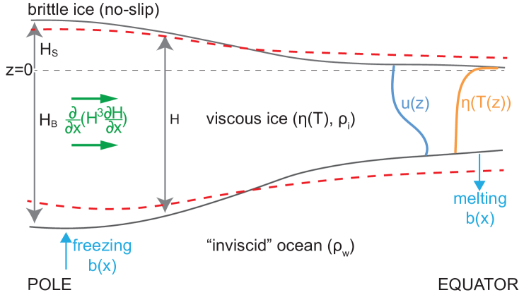
Figure 1: Schematic of ice shell flow in a 2D setup. The pole is shown on the lefthand size and equator on the righthand side of the plot. The ice thickness above sea level (at $z=0$) is $H_{S}$ and below sea level is $H_{B}$. $H=H_{S}+H_{B}$ is the total ice thickness. Viscous ice, with viscosity $\eta(T)$ and density $\rho_{i}$, sits atop an “inviscid” ocean of density $\rho_{w}$. The viscous ice shell either thins as it spreads or is sustained by freezing at the pole and melting at the equator. A new shell thickness, governed by the green nonlinear diffusive term, is shown by the dashed red line. A spatially-varying freeze/melt function is given by $b(x)$. A schematic representation of the viscosity profile $\eta(T)$ is shown in the orange line, and the resultant horizontal velocity profile $u(z)$ in the blue line.

Mathematical Formulation

The system can be described by the following equations, which generally follow the standard gravity current equations of [19] and which we extend to include the effect of a temperature-dependent viscosity. The total thickness of the ice shell is $H=H_{S}+H_{B}$, where $H_{S}$ falls above the $z=0$ sea level, and $H_{B}$ falls below the $z=0$ line. Then, $H_{S}=(1-\rho_{i}/\rho_{w})H$, where $\rho_{i}$ is the density of ice, and $\rho_{w}$ is the density of the ocean.

We start with conservation of mass: ${\frac{\partial u}{\partial x}+\frac{\partial w}{\partial z}=0}$, and conservation of momentum for Stokes flow, combined with the fact that the horizontal length scale is much larger than the vertical length scale, leading to:

$$0=-\frac{\partial p}{\partial x}+\frac{\partial}{\partial z}(\eta(T(z))\frac{\partial u}{\partial z})\textrm{, and }0=-\frac{\partial p}{\partial z}-\rho_{i}g\hat{z}\textrm{,}$$ (1)

where $p$ is pressure, $u$ is the velocity in the $x$-direction, $w$ is the velocity in the $z$-direction, $\eta(T)$ is a temperature-dependent viscosity, $\rho_{i}$ is ice density, and $g$ is gravity.

A temperature-dependent (or equivalently depth-dependent) viscosity is appropriate since the upper surface of the ice shell will be significantly colder than the base. Here we employ the Frank-Kamenetskii approximation [e.g., 32], defined as:

$$\eta(T)=\eta_{b}e^{(1/l)(1-\frac{T-T_{S}}{\Delta T})},$$ (2)

where $\eta_{b}$ is the specified basal viscosity, $\tilde{T}=\frac{T-T_{S}}{\Delta T}$, $\Delta T=T_{B}-T_{S}$, $T_{B}=273~{}K$ is the ice temperature at the ice-ocean interface, $T_{S}=93~{}K$ is the ice surface temperature [appropriate for Europa, 29], and $l=\frac{RT_{B}^{2}}{Q\Delta T}$, where $R$ is the gas constant and $Q$ is the activation energy. We note here that we take $\Delta T$ to be constant across the entire ice shell, though lateral variations in the temperature jump will exist; these are what give rise to variations in ice thickness in the first place.

The relevant boundary conditions are no-slip at the top surface (brittle lid), and free-slip (no-stress) at the ocean-ice interface, given by: $u(z=H_{S})=0$, and $\frac{\partial u}{\partial z}\rvert_{z=-H_{B}}=0$.

Then, taking $p=p_{o}+\rho_{i}g(H_{s}-z)$ yields:

$$0=-\rho_{i}g\frac{\partial H_{S}}{\partial x}+\frac{\partial}{\partial z}(\eta_{b}e^{[\frac{1}{l}(1-\frac{H_{S}-z}{H})]}\frac{\partial u}{\partial z}),$$ (3)

where $\frac{H_{S}-z}{H}=\frac{T-T_{S}}{\Delta T}$ for a linear temperature gradient across the shell.

Then, nondimensionalizing where $\tilde{z}=\frac{(H_{s}-z)}{H}$, $d\tilde{z}=-\frac{dz}{H}$, and $\tilde{u}=\frac{-u\eta_{b}e^{1/l}}{\rho_{i}gH^{2}(\partial H_{S}/\partial x)}$ gives:

$$0=1+\frac{\partial}{\partial\tilde{z}}(e^{\frac{1}{l}(1-\tilde{z})}\frac{\partial\tilde{u}}{\partial\tilde{z}}),$$ (4)

with boundary conditions:${\frac{\partial\tilde{u}}{\partial\tilde{z}}\rvert{{}_{\tilde{z}=1}}=0}$, and ${\tilde{u}(\tilde{z}=0)=0}$. This can be solved to give an analytical dimensionless velocity profile:

$$\tilde{u}=l[e^{{\tilde{z}/l}}(l+1-\tilde{z})-(l+1)]$$ (5)

Finally, depth-integrating the mass conservation equation gives:

$$\frac{\partial q}{\partial x}+\frac{\partial H}{\partial t}=b(x),$$ (6)

where $q=\int_{-H_{B}}^{H_{S}}udz$ and $b(x)$ is the source/sink term that describes background freeze and melt rates from the ocean.

This can be rewritten as:

$$\frac{\partial H}{\partial t}-\frac{\rho_{i}g}{\eta_{b}e^{1/l}}\beta\frac{\partial}{\partial x}[H^{3}\frac{\partial H_{S}}{\partial x}]-b(x)=0,$$ (7)

where $\beta=\int_{0}^{1}\tilde{u}d\tilde{z}=l[2l^{2}(e^{1/l}-1)-2l-1]$.

Finally, defining $\gamma=\beta e^{-1/l}$ and recalling that $H_{S}=(1-\rho_{i}/\rho_{w})H$, we obtain the following:

$$\frac{\partial H}{\partial t}-\frac{\rho_{i}g\gamma}{\eta_{b}}(1-\frac{\rho_{i}}{\rho_{w}})\frac{\partial}{\partial x}[H^{3}\frac{\partial H}{\partial x})]-b(x)=0,$$ (8)

This equation describes how the thickness of an ice shell with a temperature-dependent viscosity changes in time as it flows laterally and is modified by spatially-varying freezing and melting.

Results

Changes in shell thickness due to gravity-driven flattening compete with thickening and thinning of the shell due to freezing and melting of ice driven by ocean heat fluxes [see also 16, 28]. Given the temperature-dependence of viscosity and the temperature gradient across the shell, the flowing portion of the shell is confined to the bottom of the shell (Figure 2a); this can also be seen from the functional form of Equation 5. The flow rate varies in space and in time depending on the evolving local thickness gradient. It is also larger for lower basal viscosities, and smaller for higher basal viscosities. For example, for the ice shell shown here after 100 million years with a basal viscosity of 10¹⁴ Pa s, flow rates vary from approximately 0 to 2.6 mm/year (Figure 2a).

Unless sustained by ocean freezing and melting, the ice thickness will homogenize over time (Figure 2b); ice shells with lower basal viscosities flatten faster than those with larger viscosities (Figure 2c). Recent work [33] has also shown how larger effective viscosities can lead to steeper ice shell topography.

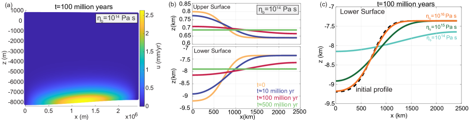
Figure 2: (a) Flow field after 100 million years for an ice shell with a temperature-dependent viscosity, with basal viscosity of $\eta_{b}=10^{14}$ Pa s. Since the bottom of the shell is warmer than the upper surface, the base is less viscous, and the flow is concentrated in this portion of the shell. For the specified basal viscosity at time $t=100$ million years, the maximum flow rate is approximately 2.6 mm/year. (b) Surface and basal topography of an ice shell, with an initial topography shown at $t=0$ (yellow), for $\eta_{b}=10^{14}$ Pa s at different times (colors). The ice shell flattens over time. (c) Basal topography of an ice shell, with an initial topography shown in (b), at different values of basal viscosity $\eta_{b}$ after 100 million years. While shells with lower viscosities have flattened, shells with higher viscosities still maintain a similar profile to the initial state.

Spatial Variation of Freeze and Melt Rates

Freezing and melting concurrent with ice flow modifies the shell-thickness distribution (Figure 3a). If ice freezes at the pole and melts at the equator at exactly the same rate as ice moves laterally between the two regions, then there will be no temporal change in ice thickness, and the ice will remain in steady-state. If Europa’s ice cover can be considered to be in steady state [e.g., 11, 34, 35, 27, 16, 28], this then provides a method by which to calculate both the spatial distribution of Europa’s ocean freeze and melt rate based on global measurements of ice thickness, as well as a way to infer the magnitudes of maximum ocean freeze/melt rates and their spatial locations. We describe how steady-state measurements of ice thickness can be used to infer information about freezing and melting in Europa’s ocean next.

The freeze/melt rate necessary to result in a steady-state ice thickness can be calculated via the following equation (see Equation 8, Figure 3b):

$$b(x)=-\frac{\rho_{i}g\gamma}{\eta_{b}}(1-\frac{\rho_{i}}{\rho_{w}})\frac{d}{dx}[H^{3}\frac{dH}{dx}]$$ (9)

The spatial location of the maximum or minimum freeze/melt rate can then be found by solving:

$$H^{3}\frac{d^{2}H}{dx^{2}}+3H^{2}(\frac{dH}{dx})^{2}=0.$$ (10)

The magnitude of the freeze and melt rate can then be determined via Equation 9. This means that a sufficiently-resolved global ice-thickness distribution $H(x)$ would indicate the locations ($x$) of maximum/minimum melt rates in an icy satellite ocean.

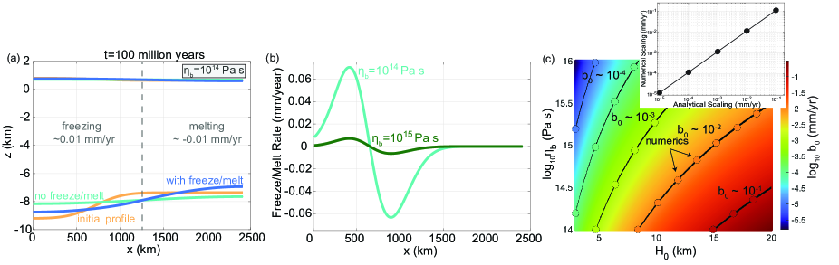
Figure 3: (a) Flow of an ice shell, with an initial thickness shown at $t=0$ (yellow), for $\eta_{b}=10^{14}$ Pa s after 100 million years both with the presence of freezing/melting (blue) and without (aqua). The ice shell flattens over time in the absence of freezing and melting, but maintains a thickness gradient when ocean freeze/melt are included. (b) Freeze and melt rate needed to maintain a steady-state thickness gradient (shown by the yellow profile in (a)). Ice shells with lower basal viscosities must have larger freeze/melt rates to offset the flow of ice. (c) Scaling for freeze/melt rate (color, mm yr^-1) of ice shell flow for different thickness scales and basal viscosities. Black lines show contours of the analytic scaling, and colored dots show the numerical freeze/melt scaling plotted on top. A linear fit between the numerical and analytic scaling show that the numerical scaling is 1.1451 times the analytic scaling (shown in the inset). The numerical scaling is based on the solution $b(x)$ from Equation 9, using the initial thickness profile shown in Figure 3a (described in the Materials and Methods section). The numerical freeze/melt rate is then taken to be the mean of the absolute values of $b(x)$.

Scalings of Ocean Dynamics

Further, how the freeze and melt rate depends on both ice shell basal viscosity, as well as ice shell thickness, can be described by a scaling law. Such a law arises by considering characteristic scales for each of the terms in Equation 8 and balancing them against each other; the scaling has the advantage of necessitating sparse ice-thickness measurements to make estimates of the freeze/melt rate and does not require a steady-state assumption. A characteristic freeze and melt rate follows:

$$b_{0}=k\frac{\gamma\rho_{i}g}{\eta_{b}}(\frac{\rho_{w}-\rho_{i}}{\rho_{w}})\frac{H_{0}^{4}}{L_{0}^{2}},$$ (11)

where $b_{0}$ is a characteristic freeze-melt scale. Here we take $L_{0}$ to be the pole-to-equator distance, $H_{0}$ to be the thickness of ice at the pole (i.e., the maximum ice thickness at any space or time), and $k$ to be a scaling prefactor. Here we find numerically $k=1.1$ (Figure 3c inset); the exact value of $k$ depends on the shape of $H(x)$. Further, recall that $\gamma=le^{-1/l}[2l^{2}(e^{1/l}-1)-2l-1]$, where $l=(RT_{B}^{2})/(Q\Delta T)$. Although we are considering a simple 1-dimensional problem here, the extension to a spherical coordinate system can be done without affecting the scaling in Equation 11.

The scaling (Equation 11) indicates that with a characteristic shell thickness scale and with a knowledge of ice viscosity, a characteristic freeze/melt rate can be inferred for the ocean. For a larger characteristic vertical thickness $H_{0}$, the characteristic freeze and melt rate $b_{0}$ will be larger than for smaller vertical thicknesses at the same viscosity (Figure 3c); this is because shells for which the value $3H^{2}(\frac{\partial H}{\partial x})^{2}+H^{3}\frac{\partial^{2}H}{\partial x}$ is larger flatten faster.

However, the ability to infer the correct magnitude of ice shell freezing and melting is dependent on a knowledge of the ice viscosity which controls how quickly the ice spreads; this is not well-prescribed [see e.g., 36]. For the same initial thickness profile, a shell with a lower basal viscosity will require a larger freeze/melt rate in order to sustain a steady-state shell thickness than a shell at larger viscosity (Figure 3b). For example, for the profile shown in Figure 3b, the maximum freeze/melt rate necessary to maintain a steady-state thickness is about 0.07 mm/year for a shell with $\eta_{b}=10^{14}$ Pa s, whereas for a shell with basal viscosity $\eta_{b}=10^{15}$ Pa s, the magnitude of the maximum freeze/melt rate necessary to maintain a steady-state is one order of magnitude smaller (about 0.007 mm/year). This is because the viscous portion of the shell will flow more slowly in the case of larger basal viscosity; thus, the rate of freezing and melting needed to offset this flow is smaller than for shells with a lower basal viscosity.

It is important to note that the ice shell viscosity does not physically determine the freeze and melt rate of the ice shell [this is governed by ocean dynamics, e.g., 27, 28], but rather that a knowledge of the ice rheology is required in order to infer an ocean freeze/melt rate based on measurements of ice thickness. Depending on the basal ice shell viscosity, varying here from 10¹⁴ to 10¹⁶ Pa s and the characteristic vertical thickness scale (which will depend on the shell profile), characteristic freeze and melt rates vary between approximately 10^-1 and 10^-5 mm/year (Figure 3c).

This means that with a spatial map of ice-thickness observations, such as is expected from Clipper or JUICE, the spatial distribution and magnitudes of ocean freeze and melt rates should be calculable under a steady-state assumption, with a knowledge of basal viscosity. Further, the locations of maximum and minimum ocean/freeze and melt rates are calculable regardless of a knowledge of basal viscosity. Finally, in the absence of a steady-state assumption, a scaling for freeze and melt rate can still be inferred from ice-thickness observations. One advantage of using this method to infer freeze/melt rate is that it may prove useful for making inferences of ocean stratification, a control on ocean dynamics of icy satellites. This is because regions of large melt rate are regions of high rates of freshwater input; here, it may be expected that a strong two-layer ocean stratification would exist [i.e., 14].

Earth Analog Radar Validation

In order to validate our methodology, we consider radar observations of an Earth analog. Radar sounding is an active remote sensing technique that has been used extensively on both Earth and Mars to measure the thickness of ice sheets and ice shelves, leveraging the relative radio-transparency of ice [37, 38, 39, 40, 41]. Figure 4a shows an example of data collected over Roosevelt Island, Antarctica as part of NASA’s Operation IceBridge that resolves the ice surface, internal reflecting horizon, and the bedrock on which the ice rise is grounded. Given the electromagnetic wave velocity in ice, spatial and temporal variations in ice thickness can be measured directly from such data. NASA’s Europa Clipper and ESA’s JUICE mission will carry similar radar sounding instruments intended to study the subsurface structure and dynamics of Europa and Ganymede’s ice shells, including ice shell thickness [42, 43]. We show that a simple scaling of the type we propose can be used to reasonably infer accumulation rates on Roosevelt Island from ice-penetrating radar measurements of the ice thickness gradient.

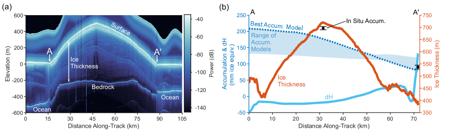
Figure 4: (a) Ice-penetrating radar data showing the cross-sectional structure of Roosevelt Island, a large grounded ice rise on the Ross Ice Shelf, Antarctica. (b) Relevant model values from observations. The region of blue shading shows the range of estimated annual accumulation rates along the transect from ERA5-Land reanalysis and the RACMO and MAR regional climate models, averaged over the last two decades. The accumulation estimate with the best match to the in situ observations (shown in the black dots) is shown in the dashed blue line. The annual rate of surface elevation change (dH) between 2008 and 2018 is shown in light blue. Surface elevation change is less than 5 cm/yr and an order of magnitude less than accumulation, suggesting that the system is in roughly steady state. Ice thickness, derived from the ice-penetrating radar profile in (a) assuming a dielectric constant of 3.15, is shown in the orange line.

Earth-analog equations

Our icy satellite case is governed by a shear flow with a no-slip upper surface, due to the extremely cold temperatures, and a free-slip base, due to the presence of the ocean. The case of Roosevelt Island, Antarctica is similar, but with a no-slip base in contact with bedrock and a free-slip surface in contact with the atmosphere. It is important to note that on Earth, the relevant flow to consider is that of an ice sheet (governed by shear flow), rather than an ice shelf [which is an extensional flow, e.g., 17, 18], even though both the Earth-based ice shelf and the ice shell of an icy satellite are floating.

The equivalent governing equation for our Earth analog is then:

$$\frac{\partial H}{\partial t}-\frac{\rho_{i}g\gamma_{e}}{\eta_{b}}\frac{\partial}{\partial x}[H^{3}\frac{\partial H}{\partial x})]-b(x)=0,$$ (12)

where now $\gamma_{e}=l[2l^{2}(1-e^{-1/l})-2l+1]$. Note that the difference between $\gamma_{e}$ in Equation 12 and $\gamma$ in Equation 8 for the icy satellite setup arises from the inverted boundary conditions. In the limit of $T_{b}=T_{s}$, $\gamma_{e}$ and $\gamma$ both reduce to 1/3.

Validation of Scaling

On Earth, the freeze/melt rate scaling goes as:

$$b_{0}\sim\frac{\rho_{i}g\gamma_{e}}{\eta_{b}}\frac{H_{0}^{4}}{L_{0}^{2}}.$$ (13)

Note the difference between this scaling and the scaling for an icy satellite, which contains a hydrostatic component related to the floating shell.

Estimates from Roosevelt Island radar observations suggest scalings of $H_{0}=750$ m and $L_{0}=35$ km (Figure 4a,b). We take $\rho_{i}=920$ kg m^-3, and $\gamma_{e}\sim 0.1-0.3$. (If the surface and basal temperatures vary by 10 Kelvin, for $T_{b}=273$ K, $\gamma_{e}\sim 0.3$, taking an activation energy $Q$ of about 60 kJ mol^-1). The viscosity of ice sheets on Earth is also not particularly well-known and much research has investigated appropriate rheology profiles for Antarctic ice sheets [e.g., 44, 45, 46]. Here, we estimate an effective viscosity of $O(10^{14})-O(10^{15})$ Pa s (see Materials & Methods); we assign this value to $\eta_{b}$. Using these parameters, we find a estimated freeze/melt scaling of $\sim 70$ mm/year for $\gamma_{e}\sim 0.1$ to $\sim 220$ mm/year for $\gamma_{e}\sim 0.3$, taking $\eta_{b}\sim O(10^{14})$. These rates fall in line with the estimated accumulation rates expected for Roosevelt Island (between about 150-200 mm year^-1 [47, 48], Figure 4b). This indicates that a scaling based on gravity-driven flow dynamics and thickness/length scale estimates may be useful for estimating accumulation rates both on Earth and on icy satellites. Similar mass-balance methodologies have also been invoked to infer melt rates at the base of Antarctic ice shelves [e.g., 49, 50, 51], further supporting this approach.

Discussion & Conclusion

Summary

On long time scales, ice flows as a viscous fluid [e.g., 17, 18]. Here we describe the dynamics of gravity-driven ice shell flow and describe how this can be used to infer melt and freeze rates under the ice shells of icy satellites, which is impossible measure directly. Since the ice shell of an icy satellite experiences a steep temperature drop from its base to its surface, and viscosity depends exponentially on temperature, we formulate the viscous gravity current equations to include a temperature-dependent viscosity. This shows analytically how the viscous flow of the ice shell is confined to its base; the thickness of the viscous portion of the shell depends on the across-shell temperature difference. In the limit of no temperature jump, our equation reduces to the classical gravity current equation with no-slip and free-slip boundary conditions [19].

We describe how a balance between ice flow and freeze and melt rate implies a scaling for freeze and melt rate which depends on a vertical ice thickness scale and a horizontal length scale. We further describe how in steady state, ocean freeze and melt rates and the spatial locations of maximum freeze and melt rates can be calculated from ice-thickness measurements. Inferences from radar observations from Roosevelt Island, Antarctica are used to corroborate our scaling and give credence to the methodology we propose. We expect that with this methodology, ocean parameters such as freeze and melt rates may be inferred with future measurements of ice thickness from upcoming space missions.

Is Europa in Steady State?

Much past work, whether considering the dynamics or thermodynamics (or both) of Europa’s ice shell, assumes that the ice shell has reached steady state [e.g., 11, 34, 35, 27, 16, 28]. Nonetheless, it is not actually clear if the shell can be considered to be in equilibrium [see 36, for a thermodynamic case].

If the steady-state assumption does not apply, then it would not be possible to directly calculate a spatially-varying freeze and melt rate as described in the previous section. However, the freeze and melt rate scaling will still be applicable provided that the term $\partial H/\partial t$ is not much larger than the nonlinear diffusive term or the freeze and melt term in Equation 8 (See Section B of Materials & Methods for more discussion). Such a system is exemplified via the radar validation of Roosevelt Island, Antarctica in the previous section which is not strictly in steady state, but for which the scaling holds. We note that at timescales appropriate for the surface age of Europa, $\partial H/\partial t$ is a similar order of magnitude to the nonlinear diffusive term for lower values of viscosity (i.e., $\sim 10^{14}$ Pa s) and larger thickness scales $H_{0}$; higher $\eta_{b}$ and lower $H_{0}$ increase the timescale of flattening for the system (see Section B of Materials & Methods).

What does Freeze and Melt Rate Tell You?

Ultimately, an understanding of ocean freeze and melt may give insight into ocean stratification. Stratification is a key control on an expected ocean circulation and thus the transport of nutrients and other tracers that may be of astrobiological interest [see 52, who describe this for the case of Enceladus]. Consider for example a region of high melt rate. This would result in a large influx of freshwater into a particular region of the ocean, likely generating a strong stratification and depressing isopycnals (surfaces of constant density). A similar description of a freshwater-stratified region and the circulation it implies via conservation of salt and heat has been described in [14]. Our methodology provides a framework to infer freeze and melt rates, which is otherwise challenging to measure under kilometers of ice, from observations of ice thickness; these rates ultimately relate to stratification.

An important point for future work is to help constrain the basal viscosity of the ice shell. This has been a limitation of modeling studies of Europa’s ice shell (including our own), as the rheology controls the relevant dynamics but is not well-defined. A particular issue is that the elastic processes on the surface can not be easily inverted via a temperature-dependence to constrain the viscous processes of the base. Developing a theoretical or observational way to constrain the basal viscosity is a key area for future research.

Materials and Methods

A. Numerical Method

Equation (8) is a one-dimensional partial differential equation that can be solved numerically subject to the following boundary conditions:

$$\frac{\partial H}{\partial x}\rvert_{x=L}=0,\textrm{no flux at the equator, and}$$ (14)

$$\int_{x=0}^{x=L}H(x,t)dx=V,\textrm{constant volume}$$ (15)

where $L$ is the end of the horizontal domain. We use a forward difference scheme in time and a centered-difference scheme in space. The spatial grid step is 10 km, and the time step is $5\times 10^{8}$ seconds. We set up a grid of 241 points, equivalent to a horizontal length of 2.4$\times$10⁶ m, approximately the distance from Europa’s pole to equator.

We approximate the initial thickness of the ice shell as complementary error function profile:

$$H(x,0)=h_{0}+a\frac{2}{\sqrt{\pi}}\int_{bx-2}^{\infty}e^{-y^{2}}dy\textrm{,}$$ (16)

where $h_{0}$ is some initial thickness, $a=h_{0}/8\sim 10^{3}$ m, and $b$ is 2.8$\times$10^-6 m^-1. The constants $h_{0}$, $a$, and $b$ can be changed to approximate different initial thickness profiles. Here we take $h_{0}=8$ km.

B. Flattening Timescale

The timescale at which an ice sheet flattens depends on the viscosity and on the thickness gradient of the ice shell. This follows the scaling law:

$$T_{0}\sim\frac{\eta_{b}}{\gamma\rho_{i}g}(\frac{\rho_{w}}{\rho_{w}-\rho_{i}})\frac{L_{0}^{2}}{H_{0}^{3}},$$ (17)

where $T_{0}$ is a characteristic time scale, $H_{0}$ is a characteristic thickness, $L_{0}$ is a characteristic horizontal length scale, $\rho_{w}$ is the density of ocean water, $\rho_{i}$ is the density of ice, $g$ is gravity, and $\eta_{b}$ is the basal ice viscosity. In order for the steady-state assumption to apply here requires $T_{0}>>H_{0}/b_{0}$ (or equivalently $T_{0}>>\frac{\eta_{b}}{\rho_{i}g\gamma}(\frac{\rho_{w}}{\rho_{w}-\rho_{i}})\frac{L_{0}^{2}}{H_{0}^{3}}$). Thus we can find a scaling for both the time at which a system subject to freezing and melting can be approximated by a steady-state, and a scaling for freeze and melt rate which would maintain the ice thickness gradient.

Our assumption of a linear temperature profile implies that possible internal shell heating does not significantly affect the temperature profile; we expect that the effect of including internal heating in our conductive setup would essentially reduce a depth-integrated viscosity in the lower portion of the shell (by keeping temperatures higher), likely leading to somewhat faster ice flow and thus increased freeze/melt rates.

C. Estimate of Viscosity

Follow the established convention in terrestrial glaciology [53, 54], we define an effective viscosity as:

$$\eta=\frac{B}{2}\dot{\epsilon}^{(1/3-1)},$$ (18)

where $\dot{\epsilon}$ is the strain rate, and $B$ is defined as ${B(T)=2.207\exp(\frac{3155}{T}-\frac{0.16612}{(273.39-T)^{1.17}})}$ [55, 56], where $T$ is temperature.

Estimates for $B(T)$ for two extreme temperatures are as follows: (1) The warmest ice is near melting temperature at $T=271$ K [57], yielding $B(T)\sim 230,000$ Pa year^1/3. (2) The surface temperature in this area is about $T=246$ K [57], yielding $B(T)\sim 800,000$ Pa year^1/3.

Finally, the order of magnitude of the effective strain rate $\dot{\epsilon}$ on Roosevelt Island as derived from satellite measurements of surface ice velocities is about 5$\times$10^-4 year^-1. Based on the upper and lower bounds of $B$, the effective viscosity can vary in the range of $\eta=6\times 10^{14}-2\times 10^{15}$ Pa s.

References

- [1] P. Cassen, R. T. Reynolds, S. Peale, Geophysical Research Letters 6, 731 (1979).
- [2] M. H. Carr, et al., Nature 391, 363 (1998).
- [3] R. T. Pappalardo, et al., Journal of Geophysical Research: Planets 104, 24015 (1999).
- [4] M. G. Kivelson, et al., Science 289, 1340 (2000).
- [5] C. C. Porco, et al., Science 311, 1393 (2006).
- [6] F. Postberg, et al., Nature 459, 1098 (2009).
- [7] L. Roth, et al., Science 343, 171 (2014).
- [8] K. P. Hand, C. F. Chyba, J. C. Priscu, R. W. Carlson, K. H. Nealson, Europa, R. T. Pappalardo, W. B. McKinnon, K. Khurana, eds. (University of Arizona Press, 2009), pp. 589–629.
- [9] G. V. Hoppa, B. R. Tufts, R. Greenberg, P. E. Geissler, Science 285, 1899 (1999).
- [10] P. M. Schenk, Nature 417, 419 (2002).
- [11] G. W. Ojakangas, D. J. Stevenson, Icarus 81, 220 (1989).
- [12] R. Pappalardo, et al., Nature 391, 365 (1998).
- [13] S. M. Howell, The Planetary Science Journal 2, 129 (2021).
- [14] P. Zhu, G. E. Manucharyan, A. F. Thompson, J. C. Goodman, S. D. Vance, Geophysical Research Letters 44, 5969 (2017).
- [15] M. Beuthe, Icarus 302, 145 (2018).
- [16] W. Kang, M. Jansen, The Astrophysical Journal 935, 103 (2022).
- [17] S. S. Pegler, M. G. Worster, Journal of Fluid Mechanics 696, 152–174 (2012).
- [18] M. G. Worster, Procedia IUTAM 10, 263 (2014).
- [19] H. E. Huppert, Journal of Fluid Mechanics 121, 43–58 (1982).
- [20] J. E. Simpson, R. E. Britter, Quarterly Journal of the Royal Meteorological Society 106, 485 (1980).
- [21] R. C. Kerr, J. R. Lister, Earth and Planetary Science Letters 85, 241 (1987).
- [22] K. N. Kowal, M. G. Worster, Journal of Fluid Mechanics 766, 626–655 (2015).
- [23] D. Stevenson, Lunar and Planetary Science Conference (2000). Abstract 1506.
- [24] F. Nimmo, Icarus 168, 205 (2004).
- [25] F. Nimmo, B. Bills, Icarus 208, 896 (2010).
- [26] S. Kamata, F. Nimmo, Icarus 284, 387 (2017).
- [27] Y. Ashkenazy, R. Sayag, E. Tziperman, Nature Astronomy 2, 43 (2018).
- [28] W. Kang, The Astrophysical Journal 934, 116 (2022).
- [29] Y. Ashkenazy, Heliyon 5, e01908 (2019).
- [30] D. L. Goldsby, D. L. Kohlstedt, Journal of Geophysical Research: Solid Earth 106, 11017 (2001).
- [31] E. L. Lewis, R. G. Perkin, Journal of Geophysical Research: Oceans 91, 11756 (1986).
- [32] C. Jain, V. S. Solomatov, Physics of Fluids 34, 096604 (2022).
- [33] M. Kihoulou, et al., Icarus 391, 115337 (2023).
- [34] H. Hussmann, T. Spohn, K. Wieczerkowski, Icarus 156, 143 (2002).
- [35] G. Tobie, G. Choblet, C. Sotin, Journal of Geophysical Research: Planets 108, 5124 (2003).
- [36] N. C. Shibley, J. Goodman (2023). Under review, arXiv:2309.16821.
- [37] S. Gogineni, et al., Journal of Geophysical Research 106, 33,761 (2001).
- [38] J. W. Holt, et al., Geophysical Research Letters 33, L09502 (2006).
- [39] D. G. Vaughan, et al., Geophysical Research Letters 33, 2 (2006).
- [40] J. J. Plaut, et al., Science 316, 92 (2007).
- [41] R. J. Phillips, et al., Science 320, 1182 (2008).
- [42] D. D. Blankenship, D. A. Young, W. B. Moore, J. C. Moore, Europa, R. T. Pappalardo, W. B. McKinnon, K. K. Khurana, eds. (University of Arizona Press, Tucson, 2017), vol. 80, pp. 631–654.
- [43] L. Bruzzone, et al., Proceedings of the IEEE 99, 837 (2011).
- [44] E. Larour, E. Rignot, I. Joughin, D. Aubry, Geophysical Research Letters 32, L05503 (2005).
- [45] J. D. Millstein, B. M. Minchew, S. S. Pegler, Communications Earth & Environment 3, 57 (2022).
- [46] Y. Wang, C.-Y. Lai, C. Cowen-Breen, under review (2023).
- [47] N. A. N. Bertler, et al., Climate of the Past 14, 193 (2018).
- [48] M. Winstrup, et al., Climate of the Past 15, 751 (2019).
- [49] J. Wen, et al., Journal of Glaciology 56, 81–90 (2010).
- [50] L. Padman, et al., Journal of Geophysical Research: Oceans 117, C01010 (2012).
- [51] S. Adusumilli, H. A. Fricker, B. Medley, L. Padman, M. R. Siegfried, Nature Geoscience 13, 616 (2020).
- [52] A. H. Lobo, A. F. Thompson, S. D. Vance, S. Tharimena, Nature Geoscience 14, 185 (2021).
- [53] J. W. Glen, Symposium de Chamonix (Association Internationale d’Hydrologie Scientifique, Chamonix, France, 1958), pp. 171–183.
- [54] J. Nye, Proceedings of the Royal Society of London. Series A. Mathematical and Physical Sciences 239, 113 (1957).
- [55] R. Hooke, Reviews of Geophysics 19, 664 (1981).
- [56] C. van der Veen, Cold Regions Science and Technology 27, 213 (1998).
- [57] R. H. Thomas, D. R. MacAyeal, C. R. Bentley, J. L. Clapp, Journal of Glaciology 25, 47 (1980/ed).