On the Parallel Complexity of Multilevel Monte Carlo
in Stochastic Gradient Descent

Abstract

In the stochastic gradient descent (SGD) for sequential simulations such as the neural stochastic differential equations, the Multilevel Monte Carlo (MLMC) method is known to offer better theoretical computational complexity compared to the naive Monte Carlo approach. However, in practice, MLMC scales poorly on massively parallel computing platforms such as modern GPUs, because of its large parallel complexity which is equivalent to that of the naive Monte Carlo method. To cope with this issue, we propose the delayed MLMC gradient estimator that drastically reduces the parallel complexity of MLMC by recycling previously computed gradient components from earlier steps of SGD. The proposed estimator provably reduces the average parallel complexity per iteration at the cost of a slightly worse per-iteration convergence rate. In our numerical experiments, we use an example of deep hedging to demonstrate the superior parallel complexity of our method compared to the standard MLMC in SGD.

1 Introduction

In this paper, we study the stochastic gradient descent (SGD) for sequential stochastic simulations such as the neural stochastic differential equations (SDEs). Since the seminal work by Chen et al. [8] on neural ordinary differential equations (ODEs), the neural differential equations have gained considerable traction in the machine learning community. The development of neural differential equations has led to various extensions beyond ODEs [8] and SDEs [37], such as neural jump ODEs [30] and SDEs [24], neural control differential equations [26], and neural stochastic partial differential equations (PDEs) [34].

In the Monte Carlo simulation of such sequential models, the multilevel Monte Carlo (MLMC) method [15, 16] is a popular choice to improve the computational complexity compared to the naive Monte Carlo approach. Notably, recent research by Ko et al. [29] explored the application of MLMC to neural SDEs, and Hu et al. [20] conducted an in-depth theoretical analysis, shedding light on the performance improvements that MLMC offers to SGD. However, when it comes to practical implementation, MLMC exhibits a scalability issue when combined with SGD on massively parallel computers such as GPUs.

In highly concurrent settings, where we can increase the batch size significantly to reduce the impact of the stochasticity in the gradient estimator during optimization, the primary bottleneck for performance shifts from standard computational complexity to the parallel complexity of the gradient estimator. In such a scenario, the limiting factor for performance becomes the total number of iterations in the SGD process, which is constrained by the parallel complexity of the gradient estimator, and consequently, the benefit of the variance reduction offered by MLMC becomes marginal. This shift poses a challenge to the effective use of MLMC within the SGD framework on high-performance parallel hardware, as the traditional MLMC estimator requires the same parallel complexity as the naive Monte Carlo estimator.

To address this issue, we propose a novel adaptation of the traditional MLMC approach, which we term "delayed MLMC." By periodically sampling the expensive parts of gradients and reusing those values for the rest of the time, the delayed MLMC achieves a substantial reduction in parallel complexity. Later in the paper, we provide theoretical analysis, where we derive the convergence rate of the SGD with the delayed MLMC for a smooth non-convex objective, and demonstrate its practical relevance by a numerical experiment using a neural SDE model.

Before delving into the technical discussions, we offer a brief comparison of our work with existing literature on variance reduction techniques for SGD. Some of the most popular variance reduction techniques such as SAG [35], SVRG [25], SAGA [10], and SPIDER [14] are orthogonal to our approach and they may be combined with our method. Still, they share a similarity with our method in that they also take advantage of the smoothness of the loss function, which requires gradients for two similar parameters to be proportionally similar. Our work aligns most closely with that of Hu et al. [20], which examines the convergence of SGD with MLMC, albeit with a primary focus on standard complexity, whereas our focus is on parallel complexity.

2 Background on Multilevel Monte Carlo Method

Here, we provide an overview of the conventional MLMC estimator of the gradient that offers better computational complexity than the naive Monte Carlo gradient estimator. Conceptually, MLMC reduces the variance of the Monte Carlo average by considering a hierarchy of the discretization size for a simulation. Instead of running the most precise but very expensive random simulations many times and taking their average, it combines the results of a large number of cheap but low-accuracy simulations with a very small number of highly accurate simulations.

To formally discuss this concept, we introduce a sequence of approximations for the true random simulation, denoted as $\{\hat{F}_{\ell}(x,\xi)\}_{\ell=0}^{{\ell_{\text{max}}}}$ along with their expectations $\{F_{\ell}(x)\}_{\ell=0}^{{\ell_{\text{max}}}}$ so that $F_{\ell}(x)=\mathbb{E}_{\xi}[\hat{F}_{\ell}(x,\xi)]$. Here, $x\in\mathbb{R}^{m}$ represents a parameter of the function and $\xi$ is a random variable. The quality of the approximation improves as we increase level $\ell$ with the maximum level offering the best possible approximation. Given such approximations, we would like to solve optimization problem

$$\operatorname*{minimize}_{x\in\mathbb{R}^{m}}F(x):=F_{\ell_{\text{max}}}(x).$$ (1)

For instance, in the case of SDEs, the approximation at level $\ell$ corresponds to the SDE simulation with step size $\Delta t=\delta 2^{-\ell}$. Although it is possible to use the naive SGD with gradient estimator $\nabla\hat{F}_{\ell_{\text{max}}}(x,\xi)$ to optimize the above objective, for many types of sequential simulations such as SDEs, it is known that we can construct a more sample efficient gradient estimator using MLMC.

For MLMC to be applicable to the problem above, we need to make additional assumptions:

Assumption 1 (Complexity of the Gradient)

Both standard and parallel complexities of estimator $\nabla\hat{F}_{\ell}$ grow exponentially to $\ell$. In other words, there exists constant $c$ such that for any $x$ and $\ell$,

$$\mathrm{Complexity}\left[\nabla\hat{F}_{\ell}(x,\xi)\right]=\mathcal{O}(2^{c\ell})\text{\ \ and \ \ }\mathrm{ParallelComplexity}\left[\nabla\hat{F}_{\ell}(x,\xi)\right]=\mathcal{O}(2^{c\ell}).$$

Furthermore, we introduce so-called coupled estimator $\Delta_{\ell}\hat{F}(x,\xi):=\hat{F}_{\ell}(x,\xi)-\hat{F}_{\ell-1}(x,\xi)$ for $\ell=0,\ldots,{\ell_{\text{max}}}$. Here, for notational simplicity, we set $\hat{F}_{-1}(x,\xi)=0$. This coupled estimator allows us to decompose original stochastic objective $\hat{F}_{\ell_{\text{max}}}(x,\xi)$ as $\hat{F}_{\ell_{\text{max}}}(x,\xi)=\sum_{\ell=0}^{\ell_{\text{max}}}\Delta_{\ell}F(x,\xi)$. Similarly, we define the difference of the expectations as $\Delta_{\ell}F(x):=F_{\ell}(x)-F_{\ell-1}(x)$. For this gradient estimator of difference $\nabla\Delta_{\ell}\hat{F}(x,\xi)$, we make the following assumption on the exponential decay of variance.

Assumption 2 (Decay of the Variance)

There exist constants $M$ and $b$ such that for any $\ell$ and $x$,

$$\mathbb{E}_{\xi}\left\|\nabla\Delta_{\ell}\hat{F}(x,\xi)-\nabla\Delta_{\ell}F(x)\right\|^{2}\leq 2^{-b\ell}M.$$

Furthermore, we assume that the decay rate of variance, represented by the parameter $b$, is faster compared to the increase rate of the cost $c$ defined in Assumption 1, so that $b>c$.

Here, to understand the feasibility of this assumption in practice, let us consider an example of an SDE simulation. In the case of SDEs, the coupled estimator corresponds to the difference between two simulations using different discretizations of the same continuous Brownian motion path $\xi$. Compared to coarse simulation $\nabla\hat{F}_{\ell-1}(x,\xi)$ in the previous level, $\nabla\hat{F}_{\ell}(x,\xi)$ uses a finer time grid with half the step size. As both of them approximate the same SDE solution given a Brownian path, the difference between them tends to decay quickly, as in the assumption.

Now, we introduce the MLMC gradient estimator with effective batch size $N$ as

$$\nabla\hat{F}_{\text{MLMC}}=\sum_{\ell=0}^{{\ell_{\text{max}}}}\frac{1}{N_{\ell}}\sum_{n=1}^{N_{\ell}}\nabla\Delta_{\ell}\hat{F}(x,\xi_{\ell,n}),$$

where $N_{\ell}=\left\lceil\frac{2^{-(b+c)\ell/2}}{\sum_{\ell=0}^{\ell_{\text{max}}}2^{-(b+c)\ell/2}}\cdot N\right\rceil=\Theta(N2^{-(b+c)\ell/2})$. This estimator has $\sum_{\ell=0}^{\ell_{\text{max}}}N_{\ell}\mathcal{O}\left(2^{c\ell}\right)=\mathcal{O}(N)$ complexity and $\sum_{\ell=0}^{\ell_{\text{max}}}\frac{M2^{-b\ell}}{N_{\ell}}=\mathcal{O}(N^{-1})$ variance due to the assumption that $b>c$. Thus, the MLMC estimator is more efficient than the naive Monte Carlo estimator

$$\nabla\hat{F}_{\text{naive}}=\frac{1}{N}\sum_{n=1}^{N}\nabla\hat{F}_{\ell_{\text{max}}}(x,\xi_{n}),$$

with $\mathcal{O}(N2^{c{\ell_{\text{max}}}})$ complexity and $\mathcal{O}(N^{-1})$ variance. In Appendix A, we describe the derivation of this optimal allocation of per-level sample size $N_{\ell}$ for MLMC that we used here.

3 Delayed Multilevel Monte Carlo method for SGD

As discussed above the MLMC estimator has superior computational complexity than the naive Monte Carlo estimator. However, the computation of the MLMC gradient always requires the computation of the highest level with $\mathcal{O}(2^{\ell_{\text{max}}})$ parallel complexity, which makes the MLMC-based SGD as slow as the naive SGD on a massively parallel computer.

To cope with this problem, we propose the delayed MLMC for SGD, which we describe in Algorithm 1, where we introduced $\nabla\Delta_{\ell}\hat{F}_{\text{MLMC}}(x,\boldsymbol{\xi}_{\ell})=\frac{1}{N_{\ell}}\sum_{n=1}^{N_{\ell}}\nabla\Delta_{\ell}\hat{F}(x,\xi_{\ell,n})$ for $\boldsymbol{\xi}_{\ell}=\left(\xi_{\ell,1},\ldots,\xi_{\ell,N_{\ell}}\right)$. With this notation, the standard MLMC estimator at step $t$ can be written as $\nabla\hat{F}_{\text{MLMC}}^{(t)}=\sum_{\ell=0}^{\ell_{\text{max}}}\nabla\Delta_{\ell}\hat{F}_{\text{MLMC}}(x_{t},\boldsymbol{\xi}_{t,\ell})$ whereas the delayed MLMC estimator becomes

$$\nabla\hat{F}_{\text{DMLMC}}^{(t)}=\sum_{\ell=0}^{{\ell_{\text{max}}}}\frac{1}{N_{\ell}}\sum_{n=1}^{N_{\ell}}\nabla\Delta_{\ell}\hat{F}_{\text{MLMC}}(x_{\tau_{\ell}(t)},\boldsymbol{\xi}_{\tau_{\ell}(t),\ell}).$$

Instead of calculating the gradient at each level every time step, the delayed MLMC estimator computes the gradient at level $\ell$ only once per every $\lfloor 2^{d\ell}\rfloor$ steps, and when the gradient computation is skipped, it reuses the most recent gradient computed at time $\tau_{\ell}(t)$, which satisfies $t-\lfloor 2^{d\ell}\rfloor\leq\tau_{\ell}(t)\leq t$ and $\tau_{\ell}(t)\equiv 0\mod\lfloor 2^{d\ell}\rfloor$. Under Assumption 1, the parallel complexities of the standard SGD and the MLMC-based SGD per iteration are both $\mathcal{O}\left(2^{c{\ell_{\text{max}}}}\right)$. In contrast, the average parallel complexity of the delayed MLMC gradient descent (Algorithm 1) per iteration is $\mathcal{O}\left(\sum_{\ell=0}^{{\ell_{\text{max}}}}2^{(c-d)\ell}\right)$, which is an improvement by a factor of $2^{d{\ell_{\text{max}}}}$ to $2^{c{\ell_{\text{max}}}}$, depending on the magnitude of $c$ and $d$. Here, a natural question to ask is to how much extent we can tolerate the bias in the gradient introduced by the delayed scheme. In the next section, we answer this question with theoretical analysis by showing that it can be controlled to negligible magnitude when learning rate $\alpha_{t}$ is taken small enough.

Initialize $x_{0}$.

for $t=0,\ldots,T$ do

       for $\ell=0,\ldots,{\ell_{\text{max}}}$ do

             if $t\equiv 0\mod\lfloor 2^{d\ell}\rfloor$ then

                   Sample a new gradient at current $x_{t}$ as $\nabla\Delta_{\ell}\hat{F}^{(t)}\leftarrow\nabla\Delta_{\ell}\hat{F}_{\text{MLMC}}(x_{t},\boldsymbol{\xi}_{t,\ell})$.

                  Update the time of the latest gradient as $\tau_{\ell}\leftarrow t$.

             end if

            

       end for

      Compute delayed gradient estimator as $\nabla\hat{F}^{(t)}_{\text{DMLMC}}\leftarrow\sum_{\ell=0}^{{\ell_{\text{max}}}}\nabla\Delta_{\ell}\hat{F}^{(\tau_{\ell})}$.

      Update the parameter $x$ as $x_{t+1}\leftarrow x_{t}-\alpha_{t}\nabla\hat{F}^{(t)}_{\text{DMLMC}}$.

end for

Algorithm 1 SGD with the delayed MLMC

4 Theoretical Guarantee

In this section, we present the results of our theoretical analysis of the delayed MLMC. To justify the skipping of gradient computation, we make the following assumption regarding smoothness.

Assumption 3 (Decay of the Smoothness)

There exist constants $L$ and $d$ such that for any $x_{1},x_{2}$ and $\ell$,

$$\left\|\nabla\Delta_{\ell}F(x_{1})-\nabla\Delta_{\ell}F(x_{2})\right\|\leq 2^{-d\ell}L\|x_{1}-x_{2}\|.$$

This assumption guarantees that gradients at higher levels undergo progressively smaller changes throughout the optimization process, enabling us to skip the computation of higher levels in the delayed MLMC. Here, note that we can trivially obtain the standard smoothness condition for SGD from this assumption as $\left\|\nabla F(x_{1})-\nabla F(x_{2})\right\|\leq\sum_{\ell=0}^{{\ell_{\text{max}}}}\left\|\nabla\Delta_{\ell}F(x_{1})-\nabla\Delta_{\ell}F(x_{2})\right\|=\sum_{\ell=0}^{{\ell_{\text{max}}}}2^{-d\ell}L\|x_{1}-x_{2}\|$. Thus, $\nabla F(x)$ is $L^{\prime}$-smooth for $L^{\prime}:=\left(\sum_{\ell=0}^{\infty}2^{-d\ell}\right)L$. With this additional assumption in place, we can now present our main theorem (with the proof available in the appendix):

Theorem 4.1 (Delayed MLMC Gradient Descent for Non-Convex Functions).

Under Assumption 2 and 3, suppose we run SGD with delayed MLMC gradient estimator $\nabla\hat{F}^{(t)}_{\text{DMLMC}}$ as in Algorithm 1. Assume that the step sizes are chosen as $\alpha_{t}=\alpha_{0}\leq\min\left\{\frac{1}{8L^{\prime}},\frac{\beta}{L}\right\}$ for $\beta$ satisfying $0<\beta\leq\frac{1}{12({\ell_{\text{max}}}+1)\left(\sum_{\ell=0}^{\infty}2^{-d\ell}\right)\log(2T+1)}$. Then, we have

$$\frac{1}{T}\sum_{t=0}^{T-1}\mathbb{E}\|\nabla F(x_{t})\|^{2}\leq\frac{8(F(x_{0})-F_{\text{inf}})}{\alpha_{0}T}+\left(24{\ell_{\text{max}}}+\frac{49}{2}\right)M^{\prime}\leq\mathcal{O}\left(\left(\frac{\log T}{T}+\frac{M}{N}\right){\ell_{\text{max}}}\right),$$

where we defined $F_{\text{inf}}:=\inf_{x}F(x)$ and $M^{\prime}:=\frac{M}{N}\left(\sum_{\ell=0}^{\ell_{\text{max}}}2^{-(b+c)\ell/2}\right)\left(\sum_{\ell=0}^{\ell_{\text{max}}}2^{-(b-c)\ell/2}\right)$.

As can be seen, our convergence rate depends on variance of the gradient $\frac{M}{N}$, but with a massively parallel computer, we can take the (effective) batch size $N$ sufficiently large to reduce the variance term to a negligible magnitude. Then, the convergence rate of delayed MLMC becomes $\mathcal{O}\left(\left(\frac{\log T}{T}\right){\ell_{\text{max}}}\right)$, which is slightly less favorable than $\mathcal{O}(\frac{1}{T})$ rate of both MLMC and naive method. At the cost of the additional factor of $\mathcal{O}\left(\log T\cdot{\ell_{\text{max}}}\right)$, the delayed MLMC gains substantial improvement in its parallel complexity as discussed earlier. For clarity, in Table 1, we provide a summarized comparison of the convergence rate and the complexities of these methods.

	Convergence rate	Complexity	Parallel complexity
Naive SGD	$\mathcal{O}(\frac{1}{T}+\frac{M}{N}{\ell_{\text{max}}})$	$\mathcal{O}(NT2^{c{\ell_{\text{max}}}})$	$\mathcal{O}(T2^{c{\ell_{\text{max}}}})$
MLMC + SGD	$\mathcal{O}(\frac{1}{T}+\frac{M}{N})$	$\mathcal{O}(NT)$	$\mathcal{O}(T2^{c{\ell_{\text{max}}}})$
Delayed MLMC + SGD (ours)	$\mathcal{O}((\frac{\log T}{T}+\frac{M}{N}){\ell_{\text{max}}})$	$\mathcal{O}(NT)$	$\mathcal{O}(T\sum_{\ell=0}^{\ell_{\text{max}}}2^{(c-d)\ell})$

Table 1: A comparison of the convergence rate of $\frac{1}{T}\sum_{t=0}^{T-1}\mathbb{E}\|\nabla F(x_{t})\|^{2}$, the (standard) complexity, and the parallel complexity of different methods. Parameters $T$, $M$, and $N$ are the number of iterations in SGD, the variance of the gradient, and the effective batch size, respectively. As $\frac{M}{N}$ can be ignored if a massively parallel computer is available to increase the batch size $N$ arbitrarily large, the leading terms become dominant in the convergence rate.

5 Experiments

In the numerical experiments, we employed an example of deep hedging [5] to assess the performance of the proposed method. In the context of deep hedging, our goal is to solve optimization problem $\min_{\theta\in\Theta,p_{0}\in\mathbb{R}}\mathbb{E}\left|\max\{S_{1}-K,0\}-\int_{0}^{1}H_{\theta}(t,S_{t})\mathrm{d}S_{t}-p_{0}\right|^{2}$, to find the optimal hedging strategy $H(t,s)$. In our experiments, we chose the underlying asset price process $S_{t}$ to be a geometric Brownian motion, and hedging strategy $H_{\theta}(t,s)$ was parameterized using a deep neural network. For more detailed information regarding the experimental setup, please refer to Appendix C.

Figure 1: The decay of squared norm of the gradient $\mathbb{E}\left\|\nabla\Delta_{\ell}\hat{F}(x,\xi)\right\|^{2}$ (left) and path-wise smoothness $\mathbb{E}\left\|\frac{\nabla\Delta_{\ell}\hat{F}(x_{t+1},\xi)-\nabla\Delta_{\ell}\hat{F}(x_{t},\xi)}{x_{t+1}-x_{t}}\right\|$ (right). These expectations were estimated by running the Monte Carlo simulation for the parameters during the optimization. The line and the band indicate the mean and standard deviation of the estimated values.

To assess the validity of Assumption 2 and 3, we examined the decay rate of the variance and the smoothness of $\nabla\Delta_{\ell}\hat{F}(x,\xi)$ during the optimization, as shown in Figure 1. To estimate the decay rate of the variance, we instead tracked squared norm of the gradient $\mathbb{E}\left\|\nabla\Delta_{\ell}\hat{F}(x,\xi_{t,\ell})\right\|^{2}$, which provides an upper bound on the variance. Since the direct estimation of the smoothness is difficult, we approximated it with the path-wise smoothness in $L^{1}$ norm. From these figures, we can reasonably assume the values of $b$ to be close to $2$ and $d$ to be $1$ in the aforementioned assumptions, which implies that the standard MLMC and the delayed MLMC are applicable to our problem.

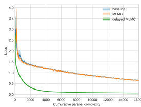
Figure 2: The mean and standard deviation of the loss throughout the optimization process for the naive SGD (baseline), the SGD with MLMC, and the SGD with delayed MLMC. Standard complexity (left) and parallel complexity (right) are used as the time scale of the learning curves. The mean and standard deviation are taken over 10 different runs.

Figure 2 illustrates the learning curves for three different optimization methods: the naive SGD (baseline), the SGD with the standard MLMC, and the SGD with delayed MLMC. All methods employed the same learning rate, and the batch sizes were adjusted to match the gradient variance across methods. When we consider parallel complexity as the horizontal axis, it becomes evident that the delayed MLMC outperforms both the baseline and the standard MLMC, which aligns with our expectations. Interestingly, even when assessing performance in terms of standard complexity as the time scale, we observe that the delayed MLMC exhibits slightly faster optimization compared to the standard MLMC. This improvement can be attributed to the skipped computation of gradients at higher levels, which again demonstrates the effectiveness of the proposed approach.

6 Conclusions

We introduced the delayed MLMC gradient estimator to address scalability challenges in MLMC for SGD on massively parallel computers. Our method demonstrates significant parallel complexity improvements in both theory and experiments compared to standard MLMC in SGD. This contribution holds great potential for enhancing the scalability of neural differential equations and related simulations in the fields of machine learning and computational science.

Appendix A A Review on the Multilevel Monte Carlo Method

A.1 Literatures on MLMC

The multilevel Monte Carlo (MLMC) method, initially introduced by Heinrich [18] for parametric integration, gained substantial recognition following the seminal work by Giles [15] on path simulation of SDEs. Its applications have since extended into various domains, including partial differential equations with random coefficients [9], continuous-time Markov chains [1], and nested simulations [6]. Following its success in the numerical simulations, the MLMC has been extended further to the fields of statistics and machine learning. In statistics, MLMC has been applied to Markov chain Monte Carlo sampling [12], sequential Monte Carlo sampling [2], particle filtering [23]. The adoption of MLMC in machine learning is a more recent development, with applications ranging from distributionally robust optimization [31] to Bayesian computation [21, 36, 32, 7] and reinforcement learning [11, 19, 38]. For those interested in a comprehensive review of MLMC, Giles [16] provides an excellent tutorial and an extensive survey.

A.2 Optimal Sample Size Allocation of MLMC

To determine the optimal sample sizes per level, denoted as $N_{0},\ldots,N_{\ell_{\text{max}}}$, we minimize the variance under a fixed total cost. For the analysis, let us assume that there exist $C,c,M$, and $b$ such that

$$C_{\ell}:=\mathrm{Complexity}\left[\nabla\Delta_{\ell}\hat{F}(x,\xi)\right]=C2^{c\ell}$$

and that

$$V_{\ell}:=\mathbb{E}\left\|\nabla\Delta_{\ell}\hat{F}(x,\xi)-\mathbb{E}\nabla\Delta_{\ell}\hat{F}(x,\xi)\right\|^{2}=M2^{-b\ell}.$$

Since the variance of the MLMC estimator $\nabla\hat{F}_{\text{MLMC}}=\sum_{\ell=0}^{{\ell_{\text{max}}}}\frac{1}{N_{\ell}}\sum_{n=1}^{N_{\ell}}\nabla\Delta_{\ell}\hat{F}_{\ell_{\text{max}}}(x,\xi_{\ell,n})$ can be written as $\sum_{\ell=0}^{\ell_{\text{max}}}\frac{V_{\ell}}{N_{\ell}}$, we can solve the following constrained optimization to obtain the optimal choice of $N_{0},\ldots,N_{\ell_{\text{max}}}$.

$$\min_{N_{0},\ldots,N_{\ell_{\text{max}}}>0}\sum_{\ell=0}^{\ell_{\text{max}}}\frac{V_{\ell}}{N_{\ell}}\text{\ \ \ \ subject to\ \ \ \ }\sum_{\ell=0}^{\ell_{\text{max}}}C_{\ell}N_{\ell}=C_{\text{total}}.$$

This problem can be solved analytically by using the method of Lagrangian multipliers, yielding the optimal sample sizes:

$$N_{\ell}=\frac{\sqrt{V_{\ell}/C_{\ell}}}{\sum_{k=0}^{\ell_{\text{max}}}\sqrt{V_{k}C_{k}}}\cdot C_{\text{total}}\propto\sqrt{\frac{V_{\ell}}{C_{\ell}}}=\mathcal{O}(2^{-(b+c)\ell/2}).$$

For this solution, the resulting optimal variance is

$$\sum_{\ell=0}^{\ell_{\text{max}}}\frac{V_{\ell}}{N_{\ell}}=\frac{1}{C_{\text{total}}}\cdot\left(\sum_{k=0}^{\ell_{\text{max}}}\sqrt{V_{k}C_{k}}\right)^{2}=\frac{1}{C_{\text{total}}}\cdot\left(\sum_{k=0}^{\ell_{\text{max}}}\mathcal{O}(2^{-(b-c)\ell/2})\right)^{2}=\mathcal{O}\left(\frac{1}{C_{\text{total}}}\right).$$

Appendix B Theoretical Analysis

Here, we provide a convergence analysis of our algorithm for smooth and non-convex objective $F(x)$. To set the stage for the analysis of the delayed MLMC, we first present a well-established result for SGD applied to smooth and non-convex objectives as a reference.

Theorem B.1 (Stochastic Gradient Descent for Non-Convex Functions [3]).

Under Assumption 2 and 3, suppose we run standard SGD with gradient estimator $\nabla\hat{F}(x_{t},\xi_{t})$ and step size $\alpha_{t}=\alpha_{0}\leq\frac{1}{L^{\prime}}$ so that $x_{t+1}\leftarrow x_{t}-\alpha_{t}\nabla\hat{F}(x_{t},\xi_{t})$ for i.i.d. samples of $\{\xi_{t}\}_{t=0}^{T-1}$. Assume the variance of the gradient is bounded so that there exists constant $M_{\nabla\hat{F}}$ such that $\mathbb{E}_{\xi}\|\nabla\hat{F}(x,\xi)-\nabla F(x)\|^{2}\leq M_{\nabla\hat{F}}$ for any $x$. Then, we have

$$\sum_{t=0}^{T-1}\alpha_{t}\left(1-\frac{L^{\prime}}{2}\alpha_{t}\right)\mathbb{E}\|\nabla F(x_{t})\|^{2}\leq F(x_{0})-F_{\text{inf}}+\sum_{t=0}^{T-1}\frac{L^{\prime}\alpha_{t}^{2}}{2}M_{\nabla\hat{F}}.$$

where we introduced $F_{\text{inf}}:=\inf F(x)$.

Proof B.2.

This proof follows Bottou et al. [3], theorem 4.10.

Also, by Assumption 3, we know that $F(x)$ is $L^{\prime}$-smooth so that

$$F(x_{t+1}) \leq F(x_{t})+\langle\nabla F(x_{t}),x_{t+1}-x_{t}\rangle+\frac{L^{\prime}}{2}\|x_{t+1}-x_{t}\|^{2}$$

$$=F(x_{t})+\langle\nabla F(x_{t}),-\alpha_{t}\nabla\hat{F}(x_{t},\xi_{t})\rangle+\frac{L^{\prime}}{2}\|-\alpha_{t}\nabla\hat{F}(x_{t},\xi_{t})\|^{2}.$$

By taking the expectation with respect to the stochasticity at time $t$ conditioned on the trajectory up to time $t-1$ (i.e. taking expectation with respect to $\xi_{t}$) and using Assumption 2, we get

$$\mathbb{E}_{\xi_{t}}F(x_{t+1}) \leq F(x_{t})+\langle\nabla F(x_{t}),-\alpha_{t}\nabla F(x_{t})\rangle+\frac{L^{\prime}\alpha_{t}^{2}}{2}\left\{\|\nabla F(x_{t})\|^{2}+\mathbb{E}_{\xi_{t}}\|\nabla\hat{F}(x_{t},\xi_{t})-\nabla F(x_{t})\|^{2}\right\}$$

$$\leq F(x_{t})-\alpha_{t}\left(1-\frac{L^{\prime}}{2}\alpha_{t}\right)\|\nabla F(x_{t})\|^{2}+\frac{L^{\prime}\alpha_{t}^{2}}{2}M_{\nabla\hat{F}}.$$

By taking the summation of $F(x_{t})-\mathbb{E}_{\xi_{t}}F(x_{t+1})+\frac{L^{\prime}\alpha_{t}^{2}}{2}M_{\nabla\hat{F}}$ for $t=0,\ldots,T-1$ and taking the (non-conditional) expectation, we get

$$\sum_{t=0}^{T-1}\alpha_{t}\left(1-\frac{L^{\prime}}{2}\alpha_{t}\right)\mathbb{E}\|\nabla F(x_{t})\|^{2} \leq F(x_{0})-\mathbb{E}F(x_{T})+\sum_{t=0}^{T-1}\frac{\alpha_{t}^{2}L^{\prime}}{2}M_{\nabla\hat{F}}$$

$$\leq F(x_{0})-F_{\text{inf}}+\sum_{t=0}^{T-1}\frac{\alpha_{t}^{2}L^{\prime}}{2}M_{\nabla\hat{F}}.$$

Remark B.3.

Here, we can substitute $M_{\nabla\hat{F}}$ with the upper bound on the variance of $\nabla\hat{F}_{\text{naive}}$ and $\nabla\hat{F}_{\text{MLMC}}$ to obtain the convergence rate in Table 1. Under Assumption 2, the variance of the naive Monte Carlo estimator can be bounded as

$$\mathbb{E}_{\xi}\|\nabla\hat{F}_{\text{naive}}(x)-\nabla F(x)\|^{2} \leq\frac{1}{N}\mathbb{E}_{\xi}\|\nabla\hat{F}_{\ell_{\text{max}}}(x,\xi)-\nabla F_{\ell_{\text{max}}}(x)\|^{2}$$

$$\leq\frac{{\ell_{\text{max}}}+1}{N}\sum_{\ell=0}^{\ell_{\text{max}}}\mathbb{E}_{\xi}\|\nabla\Delta_{\ell}\hat{F}(x,\xi)-\nabla\Delta_{\ell}F(x)\|^{2}$$

$$\leq\frac{{\ell_{\text{max}}}+1}{N}\sum_{\ell=0}^{\ell_{\text{max}}}\mathbb{E}_{\xi}\|\nabla\Delta_{\ell}\hat{F}(x,\xi)\|^{2}$$

$$\leq\frac{({\ell_{\text{max}}}+1)M}{N}\sum_{\ell=0}^{\ell_{\text{max}}}2^{-b\ell}$$

$$\leq\mathcal{O}\left(\frac{M}{N}{\ell_{\text{max}}}\right).$$

Similarly, the variance of the standard MLMC estimator can be bounded as

$$\mathbb{E}_{\xi}\|\nabla\hat{F}_{\text{MLMC}}(x)-\nabla F(x)\|^{2} =\sum_{\ell=0}^{\ell_{\text{max}}}\mathbb{E}_{\xi}\|\nabla\Delta_{\ell}\hat{F}_{\text{MLMC}}(x)-\nabla\Delta_{\ell}F(x)\|^{2}$$

$$=\sum_{\ell=0}^{\ell_{\text{max}}}\frac{1}{N_{\ell}}\mathbb{E}_{\xi}\|\nabla\Delta_{\ell}\hat{F}(x)-\nabla\Delta_{\ell}F(x)\|^{2}$$

$$=\sum_{\ell=0}^{\ell_{\text{max}}}\left\lceil\frac{2^{-(b+c)\ell/2}}{\sum_{\ell=0}^{\ell_{\text{max}}}2^{-(b+c)\ell/2}}\cdot N\right\rceil^{-1}\cdot 2^{-b\ell}M$$

$$\leq\frac{M}{N}\left(\sum_{\ell=0}^{\ell_{\text{max}}}2^{-(b+c)\ell/2}\right)\left(\sum_{\ell=0}^{\ell_{\text{max}}}2^{-(b-c)\ell/2}\right)$$

$$=\mathcal{O}\left(\frac{M}{N}\right),$$

where we used the mutual independence of coupled estimators at different levels at the first line. For notational convenience, we let $M^{\prime}:=\frac{M}{N}\left(\sum_{\ell=0}^{\ell_{\text{max}}}2^{-(b+c)\ell/2}\right)\left(\sum_{\ell=0}^{\ell_{\text{max}}}2^{-(b-c)\ell/2}\right)=M_{\nabla\hat{F}_{\text{MLMC}}}$ for the rest of the paper to represent the upper bound on the variance of the MLMC gradient estimator.

Now, to study the convergence property of the delayed MLMC, we analyze the convergence of SGD with a general biased gradient estimator.

Lemma B.4 (Biased Stochastic Gradient Descent for Non-Convex Functions).

Under Assumption 2 and 3, suppose we run SGD with a biased gradient estimator $\nabla\hat{F}^{(t)}_{\text{biased}}=\nabla\hat{F}_{\text{biased}}(x_{t},\xi_{0:t})$ depending on the information up to time $t$. Assume the variance of the biased gradient is bounded so that there exists constant $M_{\nabla\hat{F}_{\text{biased}}}$ such that $\mathbb{E}_{\xi_{t}}\|\nabla\hat{F}^{(t)}_{\text{biased}}-\mathbb{E}_{\xi_{t}}\hat{F}^{(t)}_{\text{biased}}\|^{2}\leq M_{\nabla\hat{F}_{\text{biased}}}$ holds for any $x_{0},t$, and $\xi_{0},\ldots,\xi_{t-1}$. Then, we have

$$\sum_{t=0}^{T-1}\alpha_{t}\left(\frac{1}{2}-L^{\prime}\alpha_{t}\right)\mathbb{E}\|\nabla F(x_{t})\|^{2}$$

$$\leq F(x_{0})-F_{\text{inf}}+\sum_{t=0}^{T-1}\left[\alpha_{t}\left(\frac{1}{2}+L^{\prime}\alpha_{t}\right)\mathbb{E}\|\nabla F(x_{t})-\nabla\hat{F}^{(t)}_{\text{biased}}\|^{2}+\frac{L^{\prime}M_{\nabla\hat{F}_{\text{biased}}}\alpha_{t}^{2}}{2}\right].$$

Proof B.5.

We can use a similar argument to Theorem B.1 and get

$$\mathbb{E}_{\xi_{t}}F(x_{t+1})$$

$$\leq F(x_{t})-\alpha_{t}\langle\nabla F(x_{t}),\mathbb{E}_{\xi_{t}}\nabla\hat{F}^{(t)}_{\text{biased}}\rangle+\frac{L^{\prime}}{2}\mathbb{E}_{\xi_{t}}\|-\alpha_{t}\nabla\hat{F}^{(t)}_{\text{biased}}\|^{2}$$

$$=F(x_{t})-\alpha_{t}\|\nabla F(x_{t})\|^{2}+\alpha_{t}\langle\nabla F(x_{t}),\nabla F(x_{t})-\mathbb{E}_{\xi_{t}}\nabla\hat{F}^{(t)}_{\text{biased}}\rangle$$

$$\quad\quad\quad\quad+\frac{L^{\prime}\alpha_{t}^{2}}{2}\left\{\|\mathbb{E}_{\xi_{t}}\nabla\hat{F}^{(t)}_{\text{biased}}\|^{2}+\mathbb{E}_{\xi_{t}}\|\nabla\hat{F}^{(t)}_{\text{biased}}-\mathbb{E}_{\xi_{t}}\nabla\hat{F}^{(t)}_{\text{biased}}\|^{2}\right\}$$

$$\stackrel{{\scriptstyle 2\langle v,u\rangle\leq\|v\|^{2}+\|u\|^{2}}}{{\leq}}F(x_{t})-\alpha_{t}\left(1-\frac{L^{\prime}}{2}\alpha_{t}\right)\|\nabla F(x_{t})\|^{2}+\frac{\alpha_{t}}{2}\left\{\|\nabla F(x_{t})\|^{2}+\|\nabla F(x_{t})-\mathbb{E}_{\xi_{t}}\nabla\hat{F}^{(t)}_{\text{biased}}\|^{2}\right\}$$

$$\quad\quad\quad\quad+\frac{L^{\prime}\alpha_{t}^{2}}{2}\left\{\|\mathbb{E}_{\xi_{t}}\nabla\hat{F}_{\text{biased}}^{(t)}\|^{2}-\|\nabla F(x_{t})\|^{2}+M_{\nabla\hat{F}_{\text{biased}}}\right\}$$

$$=F(x_{t})-\alpha_{t}\left(\frac{1}{2}-\frac{L^{\prime}}{2}\alpha_{t}\right)\|\nabla F(x_{t})\|^{2}+\frac{\alpha_{t}}{2}\|\nabla F(x_{t})-\mathbb{E}_{\xi_{t}}\nabla\hat{F}^{(t)}_{\text{biased}}\|^{2}$$

$$\quad\quad\quad\quad+\frac{L^{\prime}\alpha_{t}^{2}}{2}\left\{\left\langle\nabla F(x_{t})+\mathbb{E}_{\xi_{t}}\nabla\hat{F}^{(t)}_{\text{biased}},\nabla F(x_{t})-\mathbb{E}_{\xi_{t}}\nabla\hat{F}^{(t)}_{\text{biased}}\right\rangle+M_{\nabla\hat{F}_{\text{biased}}}\right\}$$

$$\stackrel{{\scriptstyle\text{Cauchy-Schwarz}}}{{\leq}}F(x_{t})-\alpha_{t}\left(\frac{1}{2}-\frac{L^{\prime}}{2}\alpha_{t}\right)\|\nabla F(x_{t})\|^{2}+\frac{\alpha_{t}}{2}\|\nabla F(x_{t})-\mathbb{E}_{\xi_{t}}\nabla\hat{F}^{(t)}_{\text{biased}}\|^{2}$$

$$\quad\quad\quad\quad+\frac{L^{\prime}\alpha_{t}^{2}}{2}\left\{\|\nabla F(x_{t})+\mathbb{E}_{\xi_{t}}\nabla\hat{F}^{(t)}_{\text{biased}}\|\cdot\|\nabla F(x_{t})-\mathbb{E}_{\xi_{t}}\nabla\hat{F}^{(t)}_{\text{biased}}\|+M_{\nabla\hat{F}_{\text{biased}}}\right\}$$

$$\stackrel{{\scriptstyle\text{triangular ineq.}}}{{\leq}}F(x_{t})-\alpha_{t}\left(\frac{1}{2}-\frac{L^{\prime}}{2}\alpha_{t}\right)\|\nabla F(x_{t})\|^{2}+\frac{\alpha_{t}}{2}\|\nabla F(x_{t})-\mathbb{E}_{\xi_{t}}\nabla\hat{F}^{(t)}_{\text{biased}}\|^{2}$$

$$\quad\quad\quad\quad+\frac{L^{\prime}\alpha_{t}^{2}}{2}\left\{\|2\nabla F(x_{t})\|\cdot\|\nabla F(x_{t})-\mathbb{E}_{\xi_{t}}\nabla\hat{F}^{(t)}_{\text{biased}}\|+\|\nabla F(x_{t})-\mathbb{E}_{\xi_{t}}\nabla\hat{F}^{(t)}_{\text{biased}}\|^{2}+M_{\nabla\hat{F}_{\text{biased}}}\right\}$$

$$\stackrel{{\scriptstyle 2ab\leq a^{2}+b^{2}}}{{\leq}}F(x_{t})-\alpha_{t}\left(\frac{1}{2}-\frac{L^{\prime}}{2}\alpha_{t}\right)\|\nabla F(x_{t})\|^{2}+\frac{\alpha_{t}}{2}\|\nabla F(x_{t})-\mathbb{E}_{\xi_{t}}\nabla\hat{F}^{(t)}_{\text{biased}}\|^{2}$$

$$\quad\quad\quad\quad+\frac{L^{\prime}\alpha_{t}^{2}}{2}\left\{\|\nabla F(x_{t})\|^{2}+2\|\nabla F(x_{t})-\mathbb{E}_{\xi_{t}}\nabla\hat{F}^{(t)}_{\text{biased}}\|^{2}+M_{\nabla\hat{F}_{\text{biased}}}\right\}$$

$$=F(x_{t})-\alpha_{t}\left(\frac{1}{2}-L^{\prime}\alpha_{t}\right)\|\nabla F(x_{t})\|^{2}+\alpha_{t}\left(\frac{1}{2}+L^{\prime}\alpha_{t}\right)\|\nabla F(x_{t})-\mathbb{E}_{\xi_{t}}\nabla\hat{F}^{(t)}_{\text{biased}}\|^{2}+\frac{L^{\prime}M_{\nabla\hat{F}_{\text{biased}}}\alpha_{t}^{2}}{2}$$

$$\stackrel{{\scriptstyle\text{Jensen's ineq.}}}{{\leq}}F(x_{t})-\alpha_{t}\left(\frac{1}{2}-L^{\prime}\alpha_{t}\right)\|\nabla F(x_{t})\|^{2}+\alpha_{t}\left(\frac{1}{2}+L^{\prime}\alpha_{t}\right)\|\nabla F(x_{t})-\nabla\hat{F}^{(t)}_{\text{biased}}\|^{2}+\frac{L^{\prime}M_{\nabla\hat{F}_{\text{biased}}}\alpha_{t}^{2}}{2}.$$

By taking the summation of the above inequalities from $t=0,\ldots,T-1$, we get the main statement.

To utilize the above lemma, we derive the upper bound on the bias term in the following.

Lemma B.6 (Bounded Bias in Delayed MLMC Gradient 1).

Under Assumption 2 and 3, suppose we run SGD with delayed MLMC gradient estimator $\nabla\hat{F}^{(t)}_{\text{DMLMC}}$ as in Algorithm 1. Then, we have

$$\mathbb{E}\|\nabla F(x_{t})-\nabla\hat{F}^{(t)}_{\text{DMLMC}}\|^{2} \leq\left\{({\ell_{\text{max}}}+1)+2\cdot\left(\sum_{\ell=0}^{{\ell_{\text{max}}}}2^{-d\ell}L\sum_{r=\tau_{\ell}(t)}^{t-1}\alpha_{r}\right)\right\}$$

$$\quad\quad\times\left\{M^{\prime}+\sum_{\ell=0}^{{\ell_{\text{max}}}}2^{-d\ell}L\sum_{s=\tau_{\ell}(t)}^{t-1}\alpha_{s}\left(\mathbb{E}\|\nabla F(x_{s})-\nabla\hat{F}^{(s)}_{\text{DMLMC}}\|^{2}+\mathbb{E}\|\nabla F(x_{s})\|^{2}\right)\right\}.$$

Proof B.7.

We will first decompose the norm of the bias as

$$\|\nabla F(x_{t})-\nabla\hat{F}^{(t)}_{\text{DMLMC}}\|$$

$$\quad=\left\|\sum_{\ell=0}^{{\ell_{\text{max}}}}\left[\nabla\Delta_{\ell}F(x_{t})-\nabla\Delta_{\ell}\hat{F}_{\text{MLMC}}(x_{\tau_{\ell}(t)},\boldsymbol{\xi}_{\tau_{\ell}(t),\ell})\right]\right\|$$

$$\quad\leq\sum_{\ell=0}^{{\ell_{\text{max}}}}\left\|\nabla\Delta_{\ell}F(x_{t})-\nabla\Delta_{\ell}\hat{F}_{\text{MLMC}}(x_{\tau_{\ell}(t)},\boldsymbol{\xi}_{\tau_{\ell}(t),\ell})\right\|$$

$$\quad\leq\sum_{\ell=0}^{{\ell_{\text{max}}}}\left\{\left\|\nabla\Delta_{\ell}F(x_{t})-\nabla\Delta_{\ell}F(x_{\tau_{\ell}(t)})\right\|+\left\|\nabla\Delta_{\ell}F(x_{\tau_{\ell}(t)})-\nabla\Delta_{\ell}\hat{F}_{\text{MLMC}}(x_{\tau_{\ell}(t)},\boldsymbol{\xi}_{\tau_{\ell}(t),\ell})\right\|\right\}.$$

By Assumption 3, we can bound the second term in the summation as

$$\left\|\nabla\Delta_{\ell}F(x_{t})-\nabla\Delta_{\ell}F(x_{\tau_{\ell}(t)})\right\|\leq 2^{-d\ell}L\|x_{t}-x_{\tau_{\ell}(t)}\|$$

and we can use the triangular inequality as

$$\|x_{t}-x_{\tau_{\ell}(t)}\| \leq\sum_{s=\tau_{\ell}(t)}^{t-1}\|x_{s+1}-x_{s}\|$$

$$\leq\sum_{s=\tau_{\ell}(t)}^{t-1}\|-\alpha_{s}\nabla\hat{F}^{(s)}_{\text{DMLMC}}\|$$

$$\leq\sum_{s=\tau_{\ell}(t)}^{t-1}\alpha_{s}\left(\|\nabla F(x_{s})-\nabla\hat{F}^{(s)}_{\text{DMLMC}}\|+\|\nabla F(x_{s})\|\right).$$

Here, we use a modified version of Cauchy-Schwarz inequality $(\sum_{i}u_{i}v_{i})^{2}\leq(\sum_{i}u_{i})^{2}(\sum_{i}v_{i}^{2})$. For non-negative $a_{i}$ and any $x_{i}$, we can show that

$$\left(\sum_{i}a_{i}x_{i}\right)^{2}\leq\left(\sum_{i}a_{i}\right)\left(\sum_{i}a_{i}x_{i}^{2}\right)$$

holds, by substituting $u_{i}=\sqrt{a_{i}}$ and $v_{i}=\sqrt{a_{i}}x_{i}$ to above. Letting $x_{i}$’s and $a_{i}$’s be the norms and their coefficients, we get

$$\mathbb{E}\|\nabla F(x_{t})-\nabla\hat{F}^{(t)}_{\text{DMLMC}}\|^{2}$$

$$\leq\mathbb{E}\Biggl{|}\sum_{\ell=0}^{{\ell_{\text{max}}}}\Biggl{\{}\left\|\nabla\Delta_{\ell}F(x_{\tau_{\ell}(t)})-\nabla\Delta_{\ell}\hat{F}_{\text{MLMC}}(x_{\tau_{\ell}(t)},\boldsymbol{\xi}_{\tau_{\ell}(t),\ell})\right\|$$

$$\quad\quad+2^{-d\ell}L\sum_{s=\tau_{\ell}(t)}^{t-1}\alpha_{s}\left(\|\nabla F(x_{s})-\nabla\hat{F}^{(s)}_{\text{DMLMC}}\|+\|\nabla F(x_{s})\|\right)\Biggr{\}}\Biggr{|}^{2}$$

$$\leq\left[\sum_{\ell=0}^{{\ell_{\text{max}}}}\left\{1+2^{-d\ell}L\sum_{s=\tau_{\ell}(t)}^{t-1}\alpha_{s}(1+1)\right\}\right]$$

$$\quad\quad\times\mathbb{E}\Biggl{[}\sum_{\ell=0}^{{\ell_{\text{max}}}}\Biggl{\{}\left\|\nabla\Delta_{\ell}F(x_{\tau_{\ell}(t)})-\nabla\Delta_{\ell}\hat{F}_{\text{MLMC}}(x_{\tau_{\ell}(t)},\boldsymbol{\xi}_{\tau_{\ell}(t),\ell})\right\|^{2}$$

$$\quad\quad\quad\quad+2^{-d\ell}L\sum_{s=\tau_{\ell}(t)}^{t-1}\alpha_{s}\left(\|\nabla F(x_{s})-\nabla\hat{F}^{(s)}_{\text{DMLMC}}\|^{2}+\|\nabla F(x_{s})\|^{2}\right)\Biggr{\}}\Biggr{]}$$

$$\leq\left\{({\ell_{\text{max}}}+1)+2\cdot\left(\sum_{\ell=0}^{{\ell_{\text{max}}}}2^{-d\ell}L\sum_{s=\tau_{\ell}(t)}^{t-1}\alpha_{s}\right)\right\}$$

$$\quad\quad\times\left\{M^{\prime}+\sum_{\ell=0}^{{\ell_{\text{max}}}}2^{-d\ell}L\sum_{s=\tau_{\ell}(t)}^{t-1}\alpha_{s}\left(\mathbb{E}\|\nabla F(x_{s})-\nabla\hat{F}^{(s)}_{\text{DMLMC}}\|^{2}+\mathbb{E}\|\nabla F(x_{s})\|^{2}\right)\right\},$$

which concludes the proof.

Now, we derive a recursive formula of the upper bound from this lemma and obtain a more concrete bound on the bias.

Lemma B.8 (Bounded Bias in Delayed MLMC Gradient 2).

Under Assumption 2 and 3, suppose we run SGD with delayed MLMC gradient estimator $\nabla\hat{F}^{(t)}_{\text{DMLMC}}$ as in Algorithm 1. Additionally, assume that step sizes are chosen as $\alpha_{t}<\frac{\beta}{L}$ for $\beta$ satisfying $0<\beta\leq\frac{1}{4({\ell_{\text{max}}}+1)\left(\sum_{\ell=0}^{\infty}2^{-d\ell}\right)\log(2T+1)}\leq\frac{1}{2}$. Then, there exist $K_{1},K_{2}>0$ such that

$$\mathbb{E}\|\nabla F(x_{t})-\nabla\hat{F}^{(t)}_{\text{DMLMC}}\|^{2}\leq K_{1}M^{\prime}+K_{2}\sum_{s=0}^{t-1}\frac{1}{t-s}\mathbb{E}\|\nabla F(x_{s})\|^{2}$$ (2)

for $t=0,\ldots,T-1$.

Proof B.9.

We first re-write the inequality in Lemma B.6 into a recursion as follows:

$$\mathbb{E}\|\nabla F(x_{t})-\nabla\hat{F}^{(t)}_{\text{DMLMC}}\|^{2}$$

$$\leq\left\{({\ell_{\text{max}}}+1)+2\cdot\left(\sum_{\ell=0}^{{\ell_{\text{max}}}}2^{-d\ell}L\sum_{r=\tau_{\ell}(t)}^{t-1}\alpha_{r}\right)\right\}$$

$$\quad\quad\times\left\{M^{\prime}+\sum_{\ell=0}^{{\ell_{\text{max}}}}2^{-d\ell}L\sum_{s=\tau_{\ell}(t)}^{t-1}\alpha_{s}\left(\mathbb{E}\|\nabla F(x_{s})-\nabla\hat{F}^{(s)}_{\text{DMLMC}}\|^{2}+\mathbb{E}\|\nabla F(x_{s})\|^{2}\right)\right\}$$

$$\leq(2\beta+1)({\ell_{\text{max}}}+1)\cdot\left\{M^{\prime}+\beta\cdot\sum_{\ell=0}^{{\ell_{\text{max}}}}2^{-d\ell}\sum_{s=\tau_{\ell}(t)}^{t-1}\left(\mathbb{E}\|\nabla F(x_{s})-\nabla\hat{F}^{(s)}_{\text{DMLMC}}\|^{2}+\mathbb{E}\|\nabla F(x_{s})\|^{2}\right)\right\}$$

$$=(2\beta+1)({\ell_{\text{max}}}+1)M^{\prime}+\beta(2\beta+1)({\ell_{\text{max}}}+1)\sum_{\ell=0}^{{\ell_{\text{max}}}}\sum_{s=t-\lfloor 2^{d\ell}\rfloor}^{t-1}2^{-d\ell}\left(\mathbb{E}\|\nabla F(x_{s})-\nabla\hat{F}^{(s)}_{\text{DMLMC}}\|^{2}+\mathbb{E}\|\nabla F(x_{s})\|^{2}\right)$$

$$\stackrel{{\scriptstyle\text{re-index}}}{{\leq}}(2\beta+1)({\ell_{\text{max}}}+1)M^{\prime}$$

$$\quad\quad\quad\quad\quad+\beta(2\beta+1)({\ell_{\text{max}}}+1)\sum_{s=0}^{t-1}\sum_{\ell=\left\lceil\frac{\log_{2}(t-s))}{d}\right\rceil}^{\infty}2^{-d\ell}\left(\mathbb{E}\|\nabla F(x_{s})-\nabla\hat{F}^{(s)}_{\text{DMLMC}}\|^{2}+\mathbb{E}\|\nabla F(x_{s})\|^{2}\right)$$

$$=(2\beta+1)({\ell_{\text{max}}}+1)M^{\prime}$$

$$\quad\quad\quad+\beta(2\beta+1)({\ell_{\text{max}}}+1)\sum_{s=0}^{t-1}2^{-d\left\lceil\frac{\log_{2}(t-s))}{d}\right\rceil}\sum_{\ell=0}^{\infty}2^{-d\ell}\left(\mathbb{E}\|\nabla F(x_{s})-\nabla\hat{F}^{(s)}_{\text{DMLMC}}\|^{2}+\mathbb{E}\|\nabla F(x_{s})\|^{2}\right)$$

$$\leq(2\beta+1)({\ell_{\text{max}}}+1)M^{\prime}$$

$$\quad\quad\quad+\beta(2\beta+1)({\ell_{\text{max}}}+1)\sum_{s=0}^{t-1}2^{-d\frac{\log_{2}(t-s))}{d}}\left(\sum_{\ell=0}^{\infty}2^{-d\ell}\right)\left(\mathbb{E}\|\nabla F(x_{s})-\nabla\hat{F}^{(s)}_{\text{DMLMC}}\|^{2}+\mathbb{E}\|\nabla F(x_{s})\|^{2}\right)$$

$$=C_{1}M^{\prime}+C_{2}\sum_{s=0}^{t-1}\frac{1}{t-s}\left(\mathbb{E}\|\nabla F(x_{s})-\nabla\hat{F}^{(s)}_{\text{DMLMC}}\|^{2}+\mathbb{E}\|\nabla F(x_{s})\|^{2}\right).$$ (3)

Here, we introduced constants $C_{1}:=(2\beta+1)({\ell_{\text{max}}}+1)$ and $C_{2}:=\beta(2\beta+1)({\ell_{\text{max}}}+1)\left(\sum_{\ell=0}^{\infty}2^{-d\ell}\right)$ at the last line. In the above reformulation, we re-indexed the summation using the fact that the summand is always non-negative and that

$$\{(\ell,s):0\leq\ell\leq{\ell_{\text{max}}},0\leq s\text{ and }t-\lfloor 2^{d\ell}\rfloor\leq s\leq t-1\}$$

$$=\{(\ell,s):0\leq\ell\leq{\ell_{\text{max}}},t-s\leq\lfloor 2^{d\ell}\rfloor\text{ and }0\leq s\leq t-1\}$$

$$\subseteq\{(\ell,s):0\leq\ell\leq{\ell_{\text{max}}},t-s\leq 2^{d\ell}\text{ and }0\leq s\leq t-1\}$$

$$\subset\{(\ell,s):(\log_{2}(t-s))/d\leq\ell\text{ and }0\leq s\leq t-1\}.$$

For notational simplicity, we used a convention of taking summation with respect to only non-negative indices in the above.

Now, we look for $K_{1},K_{2}\geq 0$ for which we can use the mathematical induction from $t=0$ to $t=T-1$ to prove (2). When $t=0$, the left-hand side of the inequality simply becomes the variance of the standard MLMC estimator as the coupled gradient estimators for all levels are calculated, making the estimator unbiased. Thus, (2) holds for any $K_{1}\geq 1$ and $K_{2}>0$ at $t=0$. Next, for the mathematical induction, let us assume that (2) holds for any $0\leq t\leq t^{\prime}-1$. Then, by (3), we get

$$\mathbb{E}\|\nabla F(x_{t})-\nabla\hat{F}^{(t)}_{\text{DMLMC}}\|^{2}$$

$$\leq C_{1}M^{\prime}+C_{2}\sum_{s=0}^{t-1}\frac{1}{t-s}\left(\mathbb{E}\|\nabla F(x_{s})-\nabla\hat{F}^{(s)}_{\text{DMLMC}}\|^{2}+\mathbb{E}\|\nabla F(x_{s})\|^{2}\right)$$

$$\leq C_{1}M^{\prime}+C_{2}\sum_{s=0}^{t-1}\frac{1}{t-s}\left(K_{1}M^{\prime}+K_{2}\sum_{u=0}^{s-1}\frac{1}{s-u}\mathbb{E}\|\nabla F(x_{u})\|^{2}+\mathbb{E}\|\nabla F(x_{s})\|^{2}\right)$$

$$=\left\{C_{1}+C_{2}K_{1}\left(\sum_{s=0}^{t-1}\frac{1}{t-s}\right)\right\}M^{\prime}+C_{2}K_{2}\sum_{s=0}^{t-1}\sum_{u=0}^{s-1}\frac{1}{(t-s)(s-u)}\mathbb{E}\|\nabla F(x_{u})\|^{2}+C_{2}\sum_{s=0}^{t-1}\frac{1}{t-s}\mathbb{E}\|\nabla F(x_{s})\|^{2}$$

$$=\left\{C_{1}+C_{2}K_{1}\left(\sum_{s=0}^{t-1}\frac{1}{t-s}\right)\right\}M^{\prime}+C_{2}K_{2}\sum_{u=0}^{t-2}\left(\sum_{s=u+1}^{t-1}\frac{1}{(t-s)(s-u)}\right)\mathbb{E}\|\nabla F(x_{u})\|^{2}$$

$$\quad\quad+C_{2}\sum_{s=0}^{t-1}\frac{1}{t-s}\mathbb{E}\|\nabla F(x_{s})\|^{2}.$$

To further the analysis, we need to bound the summation terms $\sum_{s=0}^{t-1}\frac{1}{t-s}$ and $\sum_{s=u+1}^{t-1}\frac{1}{(t-s)(s-u)}$. These terms can be bounded using the convexity of $x\mapsto\frac{1}{x}$ on domain $0<x$ and $x\mapsto\frac{1}{x(t-x)}$ on $0<x<t$ as

$$\sum_{s=0}^{t-1}\frac{1}{t-s} =\sum_{s=0}^{t-1}\frac{1}{\int_{t-s-\frac{1}{2}}^{t-s+\frac{1}{2}}x\mathrm{d}x}$$

$$\stackrel{{\scriptstyle\text{Jensen's ineq.}}}{{\leq}}\sum_{s=0}^{t-1}\int_{t-s-\frac{1}{2}}^{t-s+\frac{1}{2}}\frac{1}{x}\mathrm{d}x$$

$$=\int_{\frac{1}{2}}^{t+\frac{1}{2}}\frac{1}{x}\mathrm{d}x$$

$$=\log(2t+1)$$

and

$$\sum_{s=u+1}^{t-1}\frac{1}{(t-s)(s-u)} =\sum_{k=1}^{t-u-1}\frac{1}{k(t-u-k)}$$

$$=\sum_{k=1}^{t-u-1}\frac{1}{\left(\int_{k-\frac{1}{2}}^{k+\frac{1}{2}}x\mathrm{d}x\right)\left(t-u-\int_{k-\frac{1}{2}}^{k+\frac{1}{2}}x\mathrm{d}x\right)}$$

$$\stackrel{{\scriptstyle\text{Jensen's ineq.}}}{{\leq}}\sum_{k=1}^{t-u-1}\int_{k-\frac{1}{2}}^{k+\frac{1}{2}}\frac{\mathrm{d}x}{x(t-u-x)}$$

$$=\int_{\frac{1}{2}}^{t-u-\frac{1}{2}}\frac{\mathrm{d}x}{x(t-u-x)}$$

$$=\frac{1}{t-u}\int_{\frac{1}{2(t-u)}}^{1-\frac{1}{2(t-u)}}\frac{\mathrm{d}z}{z(1-z)}$$

$$=\frac{1}{t-u}\int_{\frac{1}{2(t-u)}}^{1-\frac{1}{2(t-u)}}\left(\frac{1}{z}+\frac{1}{1-z}\right)\mathrm{d}z$$

$$=\frac{1}{t-u}\cdot 2\log(2t-2u-1)$$

Using these bounds, we get

$$\mathbb{E}\|\nabla F(x_{t})-\nabla\hat{F}^{(t)}_{\text{DMLMC}}\|^{2}$$

$$\leq\left\{C_{1}+C_{2}K_{1}\log(2t+1)\right\}M^{\prime}+C_{2}K_{2}\sum_{u=0}^{t-2}\left(\frac{1}{t-u}\cdot 2\log(2t-2u-1)\right)\mathbb{E}\|\nabla F(x_{u})\|^{2}$$

$$\quad\quad+C_{2}\sum_{s=0}^{t-1}\frac{1}{t-s}\mathbb{E}\|\nabla F(x_{s})\|^{2}.$$

$$\leq\left\{C_{1}+C_{2}K_{1}\log(2t+1)\right\}M^{\prime}+C_{2}\left\{1+K_{2}2\log(2t-1)\right\}\sum_{s=0}^{t-1}\frac{1}{t-s}\mathbb{E}\|\nabla F(x_{s})\|^{2}.$$

$$\leq\left\{C_{1}+C_{2}K_{1}\log(2T+1)\right\}M^{\prime}+C_{2}\left\{1+K_{2}2\log(2T-1)\right\}\sum_{s=0}^{t-1}\frac{1}{t-s}\mathbb{E}\|\nabla F(x_{s})\|^{2}.$$

Therefore, by choosing

$$K_{1} =\frac{C_{1}}{1-C_{2}\log(2T+1)} =\frac{(2\beta+1)({\ell_{\text{max}}}+1)}{1-\beta(2\beta+1)({\ell_{\text{max}}}+1)\left(\sum_{\ell=0}^{\infty}2^{-d\ell}\right)\log(2T+1)}$$

and

$$K_{2} =\frac{C_{2}}{1-2C_{2}\log(2T-1)} =\frac{(2\beta+1)({\ell_{\text{max}}}+1)}{1-\beta(2\beta+1)({\ell_{\text{max}}}+1)\left(\sum_{\ell=0}^{\infty}2^{-d\ell}\right)\log(2T-1)}$$

so that $\left\{C_{1}+C_{2}K_{1}\log(2t+1)\right\}\leq K_{1}$ and $C_{2}\left\{1+K_{2}2\log(2t-1)\right\}\leq K_{2}$, we can apply mathematical induction to prove (2).

Remark B.10.

In the last part of the above proof, due to the upper bound of $\beta$ in the assumption, the denominators of $K_{1}$ and $K_{2}$ are positive because

$$1-C_{2}\log(2T-1) >1-C_{2}\log(2T+1)$$

$$\geq 1-\beta(2\beta+1)({\ell_{\text{max}}}+1)\left(\sum_{\ell=0}^{\infty}2^{-d\ell}\right)\log(2T+1)$$

$$\geq 1-\beta(2\cdot\frac{1}{2}+1)({\ell_{\text{max}}}+1)\left(\sum_{\ell=0}^{\infty}2^{-d\ell}\right)\log(2T+1)$$

$$\geq 1-\frac{1}{4({\ell_{\text{max}}}+1)\left(\sum_{\ell=0}^{\infty}2^{-d\ell}\right)\log(2T+1)}\cdot 2({\ell_{\text{max}}}+1)\left(\sum_{\ell=0}^{\infty}2^{-d\ell}\right)\log(2T+1)$$

$$=\frac{1}{2}$$

This implies that we can upper bound $K_{1}$ and $K_{2}$ as

$$K_{1} \leq 2(2\beta+1)({\ell_{\text{max}}}+1) \leq 4({\ell_{\text{max}}}+1)$$

and

$$K_{2} \leq 2\beta(2\beta+1)({\ell_{\text{max}}}+1)\left(\sum_{\ell=0}^{\infty}2^{-d\ell}\right) \leq 4\beta({\ell_{\text{max}}}+1)\left(\sum_{\ell=0}^{\infty}2^{-d\ell}\right).$$

so that the upper bounds don’t depend on $T$.

Finally, with the above bound on the bias, we obtain the main theorem:

Theorem 4.1 (Delayed MLMC Gradient Descent for Non-Convex Functions).

Under Assumption 2 and 3, suppose we run SGD with delayed MLMC gradient estimator $\nabla\hat{F}^{(t)}_{\text{DMLMC}}$ as in Algorithm 1. Assume that the step sizes are chosen as $\alpha_{t}=\alpha_{0}\leq\min\left\{\frac{1}{8L^{\prime}},\frac{\beta}{L}\right\}$ for $\beta$ satisfying $0<\beta\leq\frac{1}{12({\ell_{\text{max}}}+1)\left(\sum_{\ell=0}^{\infty}2^{-d\ell}\right)\log(2T+1)}$. Then, we have

$$\frac{1}{T}\sum_{t=0}^{T-1}\mathbb{E}\|\nabla F(x_{t})\|^{2}\leq\frac{8(F(x_{0})-F_{\text{inf}})}{\alpha_{0}T}+\left(24{\ell_{\text{max}}}+\frac{49}{2}\right)M^{\prime}.\leq\mathcal{O}\left(\left(\frac{\log T}{T}+\frac{M}{N}\right){\ell_{\text{max}}}\right).$$

Proof B.11.

By Lemma B.4 and Lemma B.8, we have

$$\sum_{t=0}^{T-1}\alpha_{0}\left(\frac{1}{2}-L^{\prime}\alpha_{0}\right)\mathbb{E}\|\nabla F(x_{t})\|^{2}$$

$$\leq F(x_{0})-F_{\text{inf}}+\sum_{t=0}^{T-1}\left[\alpha_{0}\left(\frac{1}{2}+L^{\prime}\alpha_{0}\right)\mathbb{E}\|\nabla F(x_{t})-\nabla\hat{F}^{(t)}_{\text{DMLMC}}\|^{2}+\frac{L^{\prime}M^{\prime}\alpha_{0}^{2}}{2}\right]$$

$$\leq F(x_{0})-F_{\text{inf}}+\sum_{t=0}^{T-1}\left[\alpha_{0}\left(\frac{1}{2}+\frac{1}{4}\right)\left(K_{1}M^{\prime}+K_{2}\sum_{s=0}^{t-1}\frac{1}{t-s}\mathbb{E}\|\nabla F(x_{s})\|^{2}\right)+\frac{L^{\prime}M^{\prime}\alpha_{0}^{2}}{2}\right]$$

$$\stackrel{{\scriptstyle\text{Remark \ref{rm:K1K2}}}}{{\leq}}F(x_{0})-F_{\text{inf}}+\sum_{t=0}^{T-1}\left[\alpha_{0}\cdot\frac{3}{4}\cdot 4({\ell_{\text{max}}}+1)\cdot M^{\prime}+\frac{L^{\prime}M^{\prime}\alpha_{0}^{2}}{2}\right]$$

$$\quad\quad\quad+\sum_{t=0}^{T-1}\left[\alpha_{0}\cdot\frac{3}{4}\cdot 4\beta({\ell_{\text{max}}}+1)\left(\sum_{\ell=0}^{\infty}2^{-d\ell}\right)\left(\sum_{s=0}^{t-1}\frac{1}{t-s}\mathbb{E}\|\nabla F(x_{s})\|^{2}\right)\right]$$

$$=F(x_{0})-F_{\text{inf}}+\sum_{t=0}^{T-1}\alpha_{0}\left[3({\ell_{\text{max}}}+1)+\frac{L^{\prime}}{2}\alpha_{0}\right]M^{\prime}$$

$$\quad\quad\quad+3\beta({\ell_{\text{max}}}+1)\cdot\alpha_{0}\left(\sum_{\ell=0}^{\infty}2^{-d\ell}\right)\sum_{s=0}^{T-2}\left(\sum_{t=s+1}^{T-1}\frac{1}{t-s}\right)\left(\mathbb{E}\|\nabla F(x_{s})\|^{2}\right).$$

Here, summation $\sum_{t=s+1}^{T-1}\frac{1}{t-s}$ can be bounded by Jensen’s inequality as

$$\sum_{t=s+1}^{T-1}\frac{1}{t-s} =\sum_{t=1}^{T-s-1}\frac{1}{t}$$

$$=\sum_{t=1}^{T-s-1}\frac{1}{\int_{t-\frac{1}{2}}^{t+\frac{1}{2}}x\mathrm{d}x}$$

$$\stackrel{{\scriptstyle\text{Jensen's ineq.}}}{{\leq}}\sum_{t=1}^{T-s-1}\int_{t-\frac{1}{2}}^{t+\frac{1}{2}}\frac{1}{x}\mathrm{d}x$$

$$=\int_{\frac{1}{2}}^{T-s+\frac{1}{2}}\frac{1}{x}\mathrm{d}x$$

$$=\log(2T-2s+1).$$

Thus, we get

$$\sum_{t=0}^{T-1}\alpha_{0}\left(\frac{1}{2}-L^{\prime}\alpha_{0}\right)\mathbb{E}\|\nabla F(x_{t})\|^{2}$$

$$=F(x_{0})-F_{\text{inf}}+\sum_{t=0}^{T-1}\alpha_{0}\left[3({\ell_{\text{max}}}+1)+\frac{L^{\prime}}{2}\alpha_{0}\right]M^{\prime}$$

$$\quad\quad\quad+3\beta({\ell_{\text{max}}}+1)\cdot\alpha_{0}\left(\sum_{\ell=0}^{\infty}2^{-d\ell}\right)\sum_{s=0}^{T-2}\log(2T-2s+1)\mathbb{E}\|\nabla F(x_{s})\|^{2}$$

$$\leq F(x_{0})-F_{\text{inf}}+\sum_{t=0}^{T-1}\alpha_{0}\left[3({\ell_{\text{max}}}+1)+\frac{L^{\prime}}{2}\alpha_{0}\right]M^{\prime}$$

$$\quad\quad\quad+3\beta({\ell_{\text{max}}}+1)\cdot\alpha_{0}\left(\sum_{\ell=0}^{\infty}2^{-d\ell}\right)\log(2T+1)\sum_{s=0}^{T-1}\mathbb{E}\|\nabla F(x_{s})\|^{2}$$

$$\leq F(x_{0})-F_{\text{inf}}+\sum_{t=0}^{T-1}\alpha_{0}\left[3({\ell_{\text{max}}}+1)+\frac{L^{\prime}}{2}\alpha_{0}\right]M^{\prime}$$

$$\quad\quad\quad+\frac{1}{12({\ell_{\text{max}}}+1)\left(\sum_{\ell=0}^{\infty}2^{-d\ell}\right)\log(2T+1)}\cdot 3({\ell_{\text{max}}}+1)\cdot\alpha_{0}\left(\sum_{\ell=0}^{\infty}2^{-d\ell}\right)\log(2T+1)\sum_{s=0}^{T-1}\mathbb{E}\|\nabla F(x_{s})\|^{2}$$

$$\leq F(x_{0})-F_{\text{inf}}+\sum_{t=0}^{T-1}\alpha_{0}\left[3({\ell_{\text{max}}}+1)+\frac{L^{\prime}}{2}\alpha_{0}\right]M^{\prime}+\frac{1}{4}\alpha_{0}\sum_{s=0}^{T-1}\mathbb{E}\|\nabla F(x_{s})\|^{2}.$$

Therefore, we have

$$\sum_{t=0}^{T-1}\alpha_{0}\cdot\frac{1}{8}\cdot\mathbb{E}\|\nabla F(x_{t})\|^{2} \leq\sum_{t=0}^{T-1}\alpha_{0}\left(\frac{1}{4}-L^{\prime}\alpha_{0}\right)\mathbb{E}\|\nabla F(x_{t})\|^{2}$$

$$\leq F(x_{0})-F_{\text{inf}}+\sum_{t=0}^{T-1}\alpha_{0}\left[3({\ell_{\text{max}}}+1)+\frac{L^{\prime}}{2}\alpha_{0}\right]M^{\prime}.$$

$$\leq F(x_{0})-F_{\text{inf}}+\sum_{t=0}^{T-1}\alpha_{0}\left[3({\ell_{\text{max}}}+1)+\frac{L^{\prime}}{2}\cdot\frac{1}{8L^{\prime}}\right]M^{\prime}.$$

from which the first inequality follows.

The second inequality follows trivially by substituting the upper bound on $\alpha_{0}$ to the first upper bound.

Appendix C Experimental Settings

In our numerical experiment, we employed deep hedging [5] as an example. The deep hedging involves minimization of the following objective [5, Equation 3.3]:

$$\min_{\theta\in\Theta,p_{0}\in\mathbb{R}}\mathbb{E}\left|\max\{S_{1}-K,0\}-\int_{0}^{1}H_{\theta}(t,S_{t})\mathrm{d}S_{t}-p_{0}\right|^{2}.$$

This optimization problem aims to determine optimal hedging strategy $H_{\theta}(t,s)$ and initial price $p_{0}$ of European call option with maturity at $t=1$, which is $p_{0}=\mathbb{E}\left[\max\{S_{1}-K,0\}\right]$. Hedging strategy $H_{\theta}(t,s)$ represents the amount of the underlying asset we hold to hedge against a share of sold European call option with strike price $K$, whose payoff can be written as $\max\{S_{1}-K,0\}$. For price process of the underlying asset $\{S_{t}\}_{t\in[0,1]}$, we choose geometric Brownian motion model with drift $\mu$ and volatility $\sigma$, which follows

$$\mathrm{d}S_{t}=\mu\mathrm{d}t+\sigma S_{t}\mathrm{d}B_{t}$$

for standard Brownian motion $\{B_{t}\}_{t\in[0,1]}$. To solve the SDE, we employed the Milstein scheme, a standard solver for MLMC simulation of SDEs [17]. Hedging model $H_{\theta}(t,s)$ was implemented as a feed-forward neural network with 2 hidden layers, each comprising 32 nodes. We used the SiLU activation [13] for all layers except the final layer, for which we used the sigmoid activation. This choice of activation functions ensures that the objective function is smooth and that the holding volume of the hedging strategy is within the valid range of $[0,1]$. For solving the resulting neural SDE, we used Diffrax [27], a library for neural differential equations based on Jax [4]. The parameter values for the simulation were set as follows: $c=1$, $d=1$, $b=1.8$ ${\ell_{\text{max}}}=6$, $\mu=1$, $\sigma=1$, and $K=3$.

References

- Anderson and Higham [2012] David F Anderson and Desmond J Higham. Multilevel Monte Carlo for continuous time Markov chains, with applications in biochemical kinetics. Multiscale Modeling & Simulation, 10(1):146–179, 2012.
- Beskos et al. [2017] Alexandros Beskos, Ajay Jasra, Kody Law, Raul Tempone, and Yan Zhou. Multilevel sequential Monte Carlo samplers. Stochastic Processes and their Applications, 127(5):1417–1440, 2017.
- Bottou et al. [2018] Léon Bottou, Frank E Curtis, and Jorge Nocedal. Optimization methods for large-scale machine learning. Siam Review, 60(2):223–311, 2018.
- Bradbury et al. [2018] James Bradbury, Roy Frostig, Peter Hawkins, Matthew James Johnson, Chris Leary, Dougal Maclaurin, George Necula, Adam Paszke, Jake VanderPlas, Skye Wanderman-Milne, and Qiao Zhang. JAX: composable transformations of Python+NumPy programs, 2018. URL http://github.com/google/jax.
- Buehler et al. [2019] Hans Buehler, Lukas Gonon, Josef Teichmann, and Ben Wood. Deep hedging. Quantitative Finance, 19(8):1271–1291, 2019.
- Bujok et al. [2015] Karolina Bujok, BM Hambly, and Christoph Reisinger. Multilevel simulation of functionals of Bernoulli random variables with application to basket credit derivatives. Methodology and Computing in Applied Probability, 17(3):579–604, 2015.
- Chada et al. [2022] Neil K Chada, Ajay Jasra, Kody JH Law, and Sumeetpal S Singh. Multilevel bayesian deep neural networks. arXiv preprint arXiv:2203.12961, 2022.
- Chen et al. [2018] R. T. Q. Chen, Y. Rubanova, J. Bettencourt, and D. Duvenaud. Neural Ordinary Differential Equations. In Advances in Neural Information Processing Systems 31, pages 6571–6583. Curran Associates, Inc., 2018.
- Cliffe et al. [2011] K Andrew Cliffe, Mike B Giles, Robert Scheichl, and Aretha L Teckentrup. Multilevel Monte Carlo methods and applications to elliptic PDEs with random coefficients. Computing and Visualization in Science, 14(1):3, 2011.
- Defazio et al. [2014] Aaron Defazio, Francis Bach, and Simon Lacoste-Julien. Saga: A fast incremental gradient method with support for non-strongly convex composite objectives. Advances in neural information processing systems, 27, 2014.
- Dixit and Elsheikh [2022] Atish Dixit and Ahmed Elsheikh. A multilevel reinforcement learning framework for pde based control. arXiv preprint arXiv:2210.08400, 2022.
- Dodwell et al. [2015] Tim J Dodwell, Christian Ketelsen, Robert Scheichl, and Aretha L Teckentrup. A hierarchical multilevel Markov Chain Monte Carlo algorithm with applications to uncertainty quantification in subsurface flow. SIAM/ASA Journal on Uncertainty Quantification, 3(1):1075–1108, 2015.
- Elfwing et al. [2018] Stefan Elfwing, Eiji Uchibe, and Kenji Doya. Sigmoid-weighted linear units for neural network function approximation in reinforcement learning. Neural networks, 107:3–11, 2018.
- Fang et al. [2018] Cong Fang, Chris Junchi Li, Zhouchen Lin, and Tong Zhang. Spider: Near-optimal non-convex optimization via stochastic path-integrated differential estimator. Advances in neural information processing systems, 31, 2018.
- Giles [2008a] Michael B Giles. Multilevel Monte Carlo path simulation. Operations research, 56(3):607–617, 2008a.
- Giles [2015] Michael B Giles. Multilevel Monte Carlo methods. Acta Numer., 24:259–328, 2015.
- Giles [2008b] Mike Giles. Improved multilevel Monte Carlo convergence using the Milstein scheme. In Monte Carlo and Quasi-Monte Carlo Methods 2006, pages 343–358. Springer, 2008b.
- Heinrich [2001] Stefan Heinrich. Multilevel monte carlo methods. In Large-Scale Scientific Computing: Third International Conference, LSSC 2001 Sozopol, Bulgaria, June 6–10, 2001 Revised Papers 3, pages 58–67. Springer, 2001.
- Hoerger et al. [2023] Marcus Hoerger, Hanna Kurniawati, and Alberto Elfes. Multilevel monte carlo for solving pomdps on-line. The International Journal of Robotics Research, 42(4-5):196–213, 2023.
- Hu et al. [2021] Yifan Hu, Xin Chen, and Niao He. On the bias-variance-cost tradeoff of stochastic optimization. Advances in Neural Information Processing Systems, 34:22119–22131, 2021.
- Ishikawa and Goda [2021] Kei Ishikawa and Takashi Goda. Efficient debiased evidence estimation by multilevel monte carlo sampling. In Uncertainty in Artificial Intelligence, pages 34–43. PMLR, 2021.
- JáJá [1992] Joseph JáJá. An introduction to parallel algorithms. Addison Wesley Longman Publishing Co., Inc., 1992.
- Jasra et al. [2017] Ajay Jasra, Kengo Kamatani, Kody JH Law, and Yan Zhou. Multilevel particle filters. SIAM Journal on Numerical Analysis, 55(6):3068–3096, 2017.
- Jia and Benson [2019] Junteng Jia and Austin R Benson. Neural jump stochastic differential equations. arXiv preprint arXiv:1905.10403, 2019.
- Johnson and Zhang [2013] Rie Johnson and Tong Zhang. Accelerating stochastic gradient descent using predictive variance reduction. Advances in neural information processing systems, 26, 2013.
- Kidger et al. [2020] P. Kidger, J. Morrill, J. Foster, and T. Lyons. Neural Controlled Differential Equations for Irregular Time Series. arXiv:2005.08926, 2020.
- Kidger [2021] Patrick Kidger. On Neural Differential Equations. PhD thesis, University of Oxford, 2021.
- Kloeden and Platen [1992] P. Kloeden and E. Platen. Numerical Solution of Stochastic Differential Equations. Springer, 1992.
- Ko et al. [2023] Joohwan Ko, Michael Poli, Stefano Massaroli, and Woo Chang Kim. Multilevel approach to efficient gradient calculation in stochastic systems. In ICLR 2023 Workshop on Physics for Machine Learning, 2023.
- Krach and Teichmann [2021] Calypso Herrera Florian Krach and Josef Teichmann. Neural jump ordinary differential equations: Consistent continuous-time prediction and filtering. 2021.
- Levy et al. [2020] Daniel Levy, Yair Carmon, John C Duchi, and Aaron Sidford. Large-scale methods for distributionally robust optimization. Advances in Neural Information Processing Systems, 33:8847–8860, 2020.
- Li et al. [2023] Kaiyu Li, Daniel Giles, Toni Karvonen, Serge Guillas, and François-Xavier Briol. Multilevel bayesian quadrature. In International Conference on Artificial Intelligence and Statistics, pages 1845–1868. PMLR, 2023.
- Li et al. [2020] X. Li, T.-K. L. Wong, R. T. Q. Chen, and D. Duvenaud. Scalable gradients and variational inference for stochastic differential equations. AISTATS, 2020.
- Salvi et al. [2022] Cristopher Salvi, Maud Lemercier, and Andris Gerasimovics. Neural stochastic pdes: Resolution-invariant learning of continuous spatiotemporal dynamics. Advances in Neural Information Processing Systems, 35:1333–1344, 2022.
- Schmidt et al. [2017] Mark Schmidt, Nicolas Le Roux, and Francis Bach. Minimizing finite sums with the stochastic average gradient. Mathematical Programming, 162:83–112, 2017.
- Shi and Cornish [2021] Yuyang Shi and Rob Cornish. On multilevel Monte Carlo unbiased gradient estimation for deep latent variable models. In International Conference on Artificial Intelligence and Statistics, pages 3925–3933. PMLR, 2021.
- Tzen and Raginsky [2019] B. Tzen and M. Raginsky. Neural stochastic differential equations: Deep latent Gaussian models in the diffusion limit. arXiv:1905.09883, 2019.
- Zhang et al. [2023] Dinghuai Zhang, Aaron Courville, Yoshua Bengio, Qinqing Zheng, Amy Zhang, and Ricky T. Q. Chen. Latent state marginalization as a low-cost approach for improving exploration. In The Eleventh International Conference on Learning Representations, 2023. URL https://openreview.net/forum?id=b0UksKFcTOL.