Implicit regularization of multi-task learning and finetuning in overparameterized neural networks

Abstract

It is common in deep learning to train networks on auxiliary tasks with the expectation that the learning will transfer, at least partially, to another task of interest. In this work, we investigate the inductive biases that result from learning auxiliary tasks, either simultaneously (multi-task learning, MTL) or sequentially (pretraining and subsequent finetuning, PT+FT). In the simplified setting of two-layer diagonal linear networks trained with gradient descent, we identify implicit regularization penalties associated with MTL and PT+FT, both of which incentivize feature sharing between tasks and sparsity in learned task-specific features. Notably, our results imply that during finetuning, networks operate in a hybrid of the kernel (or “lazy”) regime and the feature learning (“rich”) regime identified in prior work. Moreover, PT+FT can exhibit a novel “nested feature learning” behavior not captured by either regime, which biases it to extract a sparse subset of the features learned during pretraining. In ReLU networks, we reproduce all of these qualitative behaviors. We also observe that PT+FT (but not MTL) is biased to learn features that are correlated with (but distinct from) those needed for the auxiliary task, while MTL is biased toward using identical features for both tasks. As a result, we find that in realistic settings, MTL generalizes better when comparatively little data is available for the task of interest, while PT+FT outperforms it with more data available. We show that our findings hold qualitatively for a deep architecture trained on image classification tasks. Our characterization of the nested feature learning regime also motivates a modification to PT+FT that we find empirically improves performance. Overall, our results shed light on the impact of auxiliary task learning and suggest ways to leverage it more effectively.

1 Introduction

Neural networks are often trained on multiple tasks, either simultaneously (“multi-task learning,” henceforth MTL, see Vafaeikia et al., (2020); Zhang and Yang, (2022)) or sequentially (“pretraining” and subsequent “finetuning,” henceforth PT+FT, see Du et al., (2022); Zhou et al., (2023)). Empirically, models are able to transfer knowledge from auxiliary tasks to improve performance on tasks of interest. However, understanding of how auxiliary tasks influence learning remains limited.

Auxiliary tasks are especially useful when there is less data available for the target task. Modern “foundation models,” trained on data-rich general-purpose tasks (like next-word prediction or image generation) before adaptation to downstream tasks, are a timely example of this use case (Bommasani et al.,, 2022). Auxiliary tasks are also commonly used in reinforcement learning, where performance feedback can be scarce (Jaderberg et al.,, 2016). Intuitively, this learning strategy biases the target task solution to use representations shaped by the auxiliary task. When the tasks share common structure, this influence may enable generalization from relatively few training samples for the task of interest. However, it can also have downsides, causing a model to inherit undesirable biases from auxiliary task learning (Wang and Russakovsky,, 2023; Steed et al.,, 2022).

A relevant insight from the theoretical literature on single-task learning is the idea that a combination of initialization and learning dynamics produces an implicit regularizing effect on learned neural network solutions. This regularization can enable good generalization even when the model is overparameterized (Neyshabur,, 2017). MTL introduces the additional complexity that the solutions to each task being learned may mutually regularize one another (Ruder,, 2017). However, the form of this mutual regularization has not been characterized precisely.

In PT+FT, the effect of the auxiliary task is captured by the solution learned during pretraining, which serves as the initialization for finetuning. The effect of initialization on implicit regularization has received much study. In some settings (the so-called “lazy” or “kernel” regime), network weights deviate only slightly from initialization. In this case, the function learned by the network is linear with respect to a set of features determined at initialization, and is biased to minimize an initialization-dependent norm (Jacot et al.,, 2020; Moroshko et al.,, 2020). In the “rich” (or feature-learning) regime, networks deviate substantially from their initialization and learn data-dependent features. Feature learning is key to the generalization performance of deep networks (Vyas et al.,, 2022). However, lazy learning may also be important to the success of PT+FT, as finetuning benefits from reusing features learned during pretraining (Neyshabur,, 2017). At the same time, maintaining flexibility to learn new features may be advantageous. How these competing requirements are balanced is poorly understood. In particular, it is largely unclear whether and how learning in the rich regime still depends on the particular initialization (though see Braun et al.,, 2022).

Note that in this work, we focus on MTL in which feature extraction layers are shared and readouts are task-specific, and on PT+FT in which the readout of the network is reinitialized before finetuning.

Contributions.

In this work we characterize the inductive biases of MTL and PT+FT in terms of implicit regularization. In a simplified linear model (that importantly still captures a notion of feature learning), we provide an exact description of solutions learned by PT+FT, and an approximate description of those learned via MTL, in terms of norm minimization biases. Both biases encourage (1) the reuse of auxiliary task features and (2) sparsity in learned task-specific features. In the case of PT+FT, this bias corresponds to a hybrid of “rich” and “lazy” learning dynamics in different parts of the network. Additionally, we find that under suitable parameter scalings, PT+FT exhibits a novel “nested feature-learning” regime, distinct from the previously characterized rich and lazy regimes, which biases finetuning to extract sparse subsets of the features learned during pretraining. In ReLU networks, we reproduce all these phenomena empirically. Based on the nested feature learning insight, we suggest practical tricks to improve finetuning performance, which shows positive results in experiments. We also describe another qualitative behavior of PT+FT not captured by the linear theory: a bias toward learning main task features that are correlated with (but not necessarily identical to) those learned during pretraining, which we find is beneficial given sufficient training data for the task of interest but can be detrimental when data is scarce.

2 Related work

A variety of studies have characterized implicit regularization effects in deep learning. These include biases toward low-frequency functions (Rahaman et al.,, 2018), toward stable minima in the loss landscape (Mulayoff et al.,, 2021), toward low-rank solutions (Huh et al.,, 2023), and toward lower-order moments of the data distribution (Refinetti et al.,, 2023). In shallow (single hidden-layer) networks, Chizat and Bach, (2020) show that when using cross-entropy loss, shallow networks are biased to minimize the $\mathcal{F}_{1}$ norm, an infinite-dimensional analogue of the $\ell_{1}$ norm over the space of possible hidden-layer features (see also Lyu and Li,, 2020; Savarese et al.,, 2019). Other work has shown that implicit regularization for mean squared error loss in nonlinear networks cannot be exactly characterized as norm minimization (Razin and Cohen,, 2020), though $\mathcal{F}_{1}$ norm minimization is a precise description under certain assumptions on the inputs (Boursier et al.,, 2022).

Another line of work has explored the so-called kernel regime, in which network learning dynamics follow kernel gradient descent in function space with respect to a particular kernel (the “neural tangent kernel”) determined at network initialization (Jacot et al.,, 2020). Networks in the kernel regime fit the training data in a way that minimizes the norm in the reproducing kernel Hilbert space associated with the neural tangent kernel (Moroshko et al.,, 2020). However, other work has shown that neural network performance cannot be fully captured by the kernel regime, and instead is attributable to feature learning (Vyas et al.,, 2022). The different generalization properties of the kernel and feature-learning regimes are attributed to different associated implicit regularizers (Chizat et al.,, 2019; Fort et al.,, 2020; Bach,, 2017). Other studies (discussed in Section 3) have shown that whether a network operates in the kernel or feature-learning regimes can be controlled by the scaling of the network initialization (Chizat et al.,, 2019; Woodworth et al.,, 2020; Yang and Hu,, 2021).

Compared to the body of work on inductive biases of single-task learning, theoretical treatments of MTL and PT+FT are more scarce. Some prior studies have characterized benefits of multi-task learning with a shared representational layer in terms of an implicit bias toward shared representations (Saxe et al.,, 2022) or bounds on sample efficiency (Maurer et al.,, 2016; Wu et al.,, 2020). Others have characterized the learning dynamics of linear networks trained from nonrandom initializations, which can be applied to understand finetuning dynamics (Braun et al.,, 2022; Shachaf et al.,, 2021). However, while these works demonstrate an effect of pretrained initializations on learned solutions, the linear models they study do not capture the notion of feature learning we are interested in. A few empirical studies have compared the performance of multi-task learning vs. finetuning in language tasks, with mixed results depending on the task studied (Dery et al.,, 2021; Weller et al.,, 2022). Several authors have also observed that PT+FT outperforms PT + “linear probing” (training only the readout layer and keeping the previous layers frozen at their pretrained values), implying that finetuning benefits from the ability to learn task-specific features (Kumar et al.,, 2022; Kornblith et al.,, 2019).

3 Introduction to analysis framework: the single-task case

In much of this paper, following prior theoretical work (Woodworth et al.,, 2020; Pesme et al.,, 2021; Azulay et al.,, 2021; HaoChen et al.,, 2021; Moroshko et al.,, 2020), we study the simplified model of “diagonal linear networks,” which parameterize linear maps $f:\mathbb{R}^{d}\to\mathbb{R}$ as $f_{\vec{w}}(\vec{x})=\vec{\beta}(\vec{w})\cdot\vec{x}$ where $\vec{\beta}(\vec{w})\in\mathbb{R}^{D}$ and $\beta_{d}(\vec{w}):={w^{(2)}_{+,d}}{w^{(1)}_{+,d}}-{w^{(2)}_{-,d}}{w^{(1)}_{-,d}}$. These correspond to two-layer linear networks in which the first layer consists of one-to-one connections, with duplicate $+$ and $-$ pathways to avoid saddle point dynamics around $\vec{w}=0$. Woodworth et al., (2020) showed that overparameterized diagonal linear networks trained with gradient descent on mean squared error loss find the zero-training-error solution that minimizes $\|f\|_{\ell_{2}}^{2}=\sum_{d=1}^{D}\beta_{d}^{2}$, when trained from large initialization (the “lazy” regime, equivalent to ridge regression). When trained from small initialization, networks instead minimize $\|f\|_{\ell_{1}}=\sum_{d=1}^{D}|\beta_{d}|$ (the “rich” regime). The latter $\ell_{1}$ minimization bias is equivalent to minimizing the $\ell_{2}$ norm of the parameters $\vec{w}$ (Appendix B). This bias is a linear analogue of feature-learning, as a model with an $\ell_{1}$ penalty tends to learn solutions that depend only on a sparse set of input dimensions (i.e. features).

To observe the link between implicit regularization and generalization performance, we train diagonal linear networks in a teacher-student setting. We consider linear regression tasks with high-dimensional input and scalar output, defined by ground-truth weights $\vec{w}\in\mathbb{R}^{1000}$. We vary the number of nonzero ground-truth weights in a task; conditioned on a weight being nonzero, its value is sampled from $\{-1,1\}$. We use 1024 auxiliary task samples and vary the number of main task samples, with all inputs sampled uniformly over the unit sphere. Additionally, we always train to a fixed, small value of the training loss ($10^{-10}$ for linear experiments, $10^{-8}$ for ReLU experiments), so that our results illustrate generalization behavior rather than optimization behavior. To expose lazy and rich learning regimes, we initialize the parameters of the diagonal linear networks at $1.0$ and $10^{-3}$, respectively. We see that rich-regime networks learn solutions with smaller $\ell_{1}$ norm (and larger $\ell_{2}$ norm), (Fig. 1a), resulting in better generalization performance on a task with sparse ground-truth weights (but not on a task with dense ground-truth weights) (Fig. 1b).

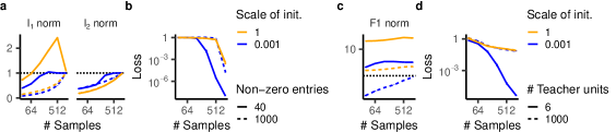
Figure 1: Single-task learning. a, $\ell_{1}$ and $\ell_{2}$ norm (relative to norm of the ground truth target, indicated by a dashed horizontal line) and b, generalization loss (mean squared error, on test data) of diagonal linear networks. The x-axis is log scaled. c, $\mathcal{F}_{1}$ norm (relative to ground truth) and d, generalization loss of shallow ReLU networks trained on data from a ReLU teacher network.

Similar analyses can be performed with nonlinear networks. Shallow ReLU networks are biased to minimize the $\mathcal{F}_{1}$ norm in the case of cross-entropy loss (Chizat and Bach, (2020), and see Boursier et al., (2022) for a result for mean squared error under assumptions on the inputs). The $\mathcal{F}_{1}$ norm is an analogue of the $\ell_{1}$ norm over the infinite-dimensional space of ReLU features, and its minimization encourages learning a solution that relies on a sparse set of features. For a network with $H$ hidden units parameterized as $f_{\vec{w}}(x)=\sum_{h=1}^{H}w^{(2)}_{h}(\langle\vec{w}^{(1)}_{h},\vec{x}\rangle)_{+}$, minimizing the $\mathcal{F}_{1}$ norm $\|f\|_{\mathcal{F}_{1}}:=\sum_{h=1}^{H}|w^{(2)}|\|w^{(1)}_{h}\|_{2}$ is equivalent to minimizing the parameters’ combined $\ell_{2}$ norm, $\|w^{(1)}\|_{2}^{2}+\|w^{(2)}\|_{2}^{2}$ (Nacson et al.,, 2019; Lyu and Li,, 2020). To test this description of the inductive bias of ReLU networks, we perform experiments with a ground-truth function parameterized by a single-hidden-layer teacher network with ReLU units, Gaussian random input weights, and binary $\pm 1$ outputs. We train a shallow overparameterized student network with 1000 hidden units on teacher-generated data. We confirm that the network with small initialization finds a solution with smaller $\mathcal{F}_{1}$ norm than the network with large initialization (Fig. 1c) and consequently generalizes better when the ground-truth teacher uses a sparse set of features, but not when the ground-truth teacher uses many features (Fig. 1d).

4 Inductive biases of PT+FT and MTL (linear theory)

4.1 Finetuning combines rich and lazy learning

We now consider the behavior of PT+FT in overparameterized diagonal linear networks. The dynamics of the pretraining and finetuning steps can each be described by the techniques of Woodworth et al., (2020) and Azulay et al., (2021). We combine these steps, using the first-layer weights from the pretraining solution as the initialization for finetuning and re-initializing the readout weights with constant magnitude $\gamma$. We find (see Appendix A) that PT+FT minimizes the following penalty on solutions $\vec{\beta}\in\mathbb{R}^{D}$ (henceforth, the “Q penalty”):

$$\textstyle\|\vec{\beta}\|_{Q}:=\sum_{d=1}^{D}\left(|\beta_{d}^{aux}|+\gamma^{2}\right)q\left(\frac{2\beta_{d}}{|\beta_{d}^{aux}|+\gamma^{2}}\right),\qquad q(z)=2-\sqrt{4+z^{2}}+z\cdot\textrm{arcsinh}(z/2)$$ (1)

It is informative to consider limits of this expression. As $\frac{|\beta_{d}|}{|\beta_{d}^{aux}|+\gamma^{2}}\to\infty$, the contribution of a feature $d$ approaches $c|\beta_{d}|$ where $c\sim\mathcal{O}\left(\log\left(1/(|\beta_{d}^{aux}|+\gamma^{2})\right)\right)$. As $\frac{|\beta_{d}|}{|\beta_{d}^{aux}|+\gamma^{2}}\to 0$, the contribution converges to $\beta_{d}^{2}/|\beta_{d}^{aux}|$. Thus, for features that are weighted sufficiently strongly by the auxiliary task (large $|\beta_{d}^{aux}|$), finetuning minimizes a weighted $\ell_{2}$ penalty that encourages reuse of features in proportion to their auxiliary task weight. For features specific to the auxiliary task (low $|\beta_{d}^{aux}|$), finetuning is biased to minimize an $\ell_{1}$ penalty, encouraging sparsity in task-specific features. Overall, the penalty decreases with $|\beta_{d}^{aux}|$, encouraging feature reuse where possible. The combination of $\ell_{1}$ and $\ell_{2}$ behavior, as well as the dependence on $|\beta_{d}^{aux}|$, can be observed in Fig. 2a (left panel).

4.2 Multi-task training learns sparse and shared features

Now we consider MTL for diagonal linear networks. A multi-output diagonal linear network with $O$ outputs can be written as: $f_{\vec{w}}(\vec{x})=\beta(\vec{w})\vec{x},$ where $\beta(\vec{w})\in\mathbb{R}^{O\times D}$, $\vec{\beta}_{o}(\vec{w}):=\vec{w}^{(2)}_{+,o}\circ\vec{w}^{(1)}_{+}-\vec{w}^{(2)}_{-,o}\circ\vec{w}^{(1)}_{-}$ (where $\circ$ is elementwise multiplication). We consider the effect of minimizing $\|\vec{w}\|_{2}$ in the MTL case, as an approximation of the inductive bias of training a network from small initialization. We make a few comments about this assumption. First, it can be proven in the case of cross-entropy loss that training dynamics decrease $\|\vec{w}\|_{2}$ (Lyu and Li,, 2020). Second, for mean squared error loss, the analogous result ($\|\vec{w}\|_{2}$ minimization) holds for diagonal linear networks in the single-output case (Woodworth et al.,, 2020). Finally, explicit $\ell_{2}$ parameter norm regularization (“weight decay”) is commonly used in neural network training, and parameter norm minimization characterizes the bias of such a training strategy.

We show (see Appendix B) that in MTL, a parameter norm minimization bias translates to minimizing an $\ell_{1,2}$ penalty that incentivizes group sparsity (Yuan and Lin,, 2006) on the learned linear map $\beta$: $\|\beta\|_{1,2}:=2\sum_{d=1}^{D}\|\vec{\beta}_{\cdot,d}\|_{2}$. For two outputs, $O=2$, $\|\cdot\|_{1,2}$ is given by

$$\textstyle\|\beta\|_{1,2}=2\sum_{d=1}^{D}\sqrt{(\beta_{d}^{aux})^{2}+(\beta_{d})^{2}},$$ (2)

where we have labeled one of the two tasks as the auxiliary (“aux”) task. To our knowledge, this is a novel description of the inductive bias of MTL in neural networks. Note that a formally similar $\ell_{1,2}$ penalty has previously been used in a single-task setting to describe group lasso penalty that groups together partitions of feature space defined by the input data points (Wang and Lin,, 2021; Pilanci and Ergen,, 2020; Wang et al.,, 2022). However, our usage of the $\ell_{1,2}$ norm is qualitatively different, as it relates to feature sharing across tasks.

This penalty (plotted in Fig. 2a, right panel), encourages using shared features for the main and auxiliary tasks, as the contribution of $\beta_{d}$ to the square-root expression is smaller when $\beta_{d}^{aux}$ is large. As $\frac{|\beta_{d}|}{|\beta_{d}^{aux}|+\gamma^{2}}\to\infty$, the penalty converges to $2|\beta_{d}|$, a sparsity-inducing $\ell_{1}$ bias for task-specific features. As $\frac{|\beta_{d}|}{|\beta_{d}^{aux}|+\gamma^{2}}\to 0$ it converges to $\frac{\beta_{d}^{2}}{|\beta_{d}^{aux}|}$, a weighted $\ell_{2}$ bias as in the PT+FT case.

4.3 Comparison of the MTL and PT+FT biases

The MTL and PT+FT penalties have many similarities. Both decrease as $|\beta_{d}^{aux}|$ increases, both are proportional to $|\beta_{d}|$ as $\frac{|\beta_{d}|}{|\beta_{d}^{aux}|+\gamma^{2}}\to\infty$, and both are proportional to $\frac{\beta_{d}^{2}}{|\beta_{d}^{aux}|}$ as $\frac{|\beta_{d}|}{|\beta_{d}^{aux}|+\gamma^{2}}\to 0$. These similarities are evident in Fig. 2a. However, two differences between the penalties merit attention.

First, the relative weights of the $\ell_{1}$ and weighted $\ell_{2}$ penalties are different between MTL and PT+FT. In particular, in the $\ell_{1}$ penalty limit, there is an extra factor of order $\mathcal{O}\left(\log\left(1/(|\beta_{d}^{aux}|+\gamma^{2})\right)\right)$ in the PT+FT penalty. Assuming small initializations, this factor tends to be larger than $2$, the corresponding coefficient in the MTL penalty. Thus, PT+FT is more strongly biased toward reusing features from the auxiliary task (i.e. features where $|\beta_{d}^{aux}|\gg 0$) compared to MTL. We are careful to note, however, that in the case of nonlinear networks this effect is complicated by a qualitatively different phenomenon with effects in the reverse direction (see Section 6.2).

Second, the two norms behave differently for intermediate values of $\frac{\beta_{d}}{|\beta_{d}^{aux}|}$. In particular, as $\beta_{d}$ increases beyond the value of $\beta_{d}^{aux}$, the MTL norm quickly grows insensitive to the value of $\beta_{d}^{aux}$ (Fig. 2a, right panel.). On the other hand, the PT+FT penalty remains sensitive to the value of $\beta_{d}^{aux}$ even for fairly large values of $\beta_{d}$, well into the $\ell_{1}$-like penalty regime (Fig. 2a, left panel). This property of the PT+FT norm, in theory, can enable finetuned networks to exhibit a rich regime-like sparsity bias while remaining influenced by their initializations. We explore this effect in Section 5.2.

5 Verification and implications of the linear theory

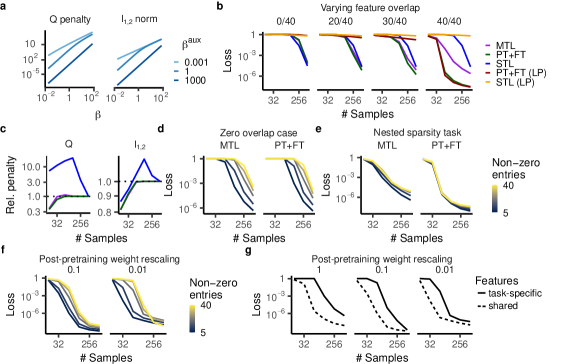
Figure 2: Diagonal linear networks. a: $Q$ (Eq. 1) and $\ell_{1,2}$ (Eq. 2) penalties, assuming negligible $\gamma$ for the $Q$ penalty. Log scale on both axes. b: Main task generalization loss for networks trained with MTL, PT+FT, single-task learning (STL), PT + finetuning via linear probing (PT+FT (LP)), and single-task linear probing (STL (LP), equivalent to lazy single-task learning, or ridge regression). Log scale on both axes. c: $\ell_{1,2}$ norm and $Q$ penalty for MTL, STL, and PT+FT networks from panel b (40/40 case). d: Generalization loss for case in which auxiliary task (with 40 nonzero ground-truth weights) and main task (number of ground-truth weights indicated by color scale) share no common features. e: Generalization loss for case in which main task uses a subset of the features used by the auxiliary task. f: Same as PT+FT case in panel e, but with the network weights rescaled by 0.1 or 0.01 (panel title) following pretraining. A sparsity bias is evident, unlike in e (rescaling = 1.0 case), and more pronounced as rescaling coefficient decreases. g: Performance in the case of 5 main task features chosen either as a subset of the auxiliary task features (“shared”) or disjoint from them (“task-specific”), varying the rescaling of weights following pretraining (1, 0.1, and 0.01). A bias toward feature reuse is evident even at the low scalings which yield a sparsity bias in panel f.

To validate these theoretical findings and illustrate their consequences, we performed experiments with diagonal linear networks in a teacher-student setup. As in Section 3, we consider linear regression tasks defined by weights $\vec{w}\in\mathbb{R}^{1000}$ with a sparse set of $k$ non-zero entries. We sample two such vectors, corresponding to “auxiliary” and “main” tasks, varying the number of nonzero entries $k_{aux}$ and $k_{main}$ and the extent to which the tasks share features (number of overlapping nonzero entries). We then train diagonal linear networks on data generated from these ground-truth weights, using 1024 auxiliary task samples and varying the number of main task samples. For re-initialization of the readout, we use $\gamma=10^{-3}$.

5.1 Feature reuse and sparse task-specific feature learning in PT+FT and MTL

We begin with tasks in which $k_{aux}=k_{main}=40$ (both tasks use the same number of features), varying the overlap between the feature sets (Fig. 2b). Both MTL and PT+FT display greater sample efficiency than single-task learning when the feature sets overlap. This behavior is consistent with an inductive bias towards feature sharing. Additionally, both MTL and PT+FT substantially outperform single-task lazy-regime learning, and nearly match single-task rich-regime learning, when the feature sets are disjoint. This is consistent with the $\ell_{1}$-like biases for task-specific features derived above, which coincide with the bias of single-task rich-regime (but not lazy-regime) learning. When the tasks partially overlap, MTL and PT+FT outperform both single-task learning and a PT + linear probing strategy, which by construction cannot learn task-specific features. This demonstrates that both PT+FT and MTL are capable of simultaneously exhibiting a bias towards feature sharing while also displaying rich regime-like task-specific feature learning, consistent with the hybrid $\ell_{1}$ / weighted-$\ell_{2}$ regularization penalties derived above. Interestingly, PT+FT performs better than MTL when the tasks use identical feature sets. This behavior is consistent with the $Q$-norm more strongly penalizing new-feature learning than the MTL norm, as observed in Section 4.3.

To check whether the implicit regularization theory is a good explanation for these performance results, we directly measured the $\ell_{1,2}$ and $Q$ norms of the solutions learned by networks, compared to the corresponding penalties of the ground truth weights. In Fig. 2c we see that as the amount of training data increases, the norms all converge to that of the ground truth solution, but in the low-sample regime, MTL and PT+FT find solutions with lower values of their corresponding norm than the ground-truth function, consistent with the implicit regularization picture (by contrast, STL does not consistently find solutions with lower values of these norms than the ground truth).

Another key prediction of the theory is that both PT+FT and MTL exhibit a sparsity bias when learning task-specific features, as both associated penalties are proportional to an $\ell_{1}$ norm when $|\beta_{d}|\gg|\beta_{d}^{aux}|$. To test this, we conducted experiments in which the main and auxiliary task features do not overlap, and varied the number $k_{main}$ of main task features. We find that both MTL and PT+FT are more sample-efficient when the main task is sparser, consistent with the prediction (Fig. 2d).

5.2 PT+FT exhibits a novel scaling-dependent nested feature-learning regime

In the limit of small $\frac{|\beta_{d}|}{|\beta_{d}^{aux}|}$, both the MTL and PT+FT penalties converge to weighted $\ell_{2}$ norms. Notably, the behavior is $\ell_{2}$-like even when $\frac{|\beta_{d}|}{|\beta_{d}^{aux}|}\approx 1$ (Fig. 2a). Thus, among features that are weighted as strongly in the auxiliary task as the main task, the theory predicts that PT+FT and MTL should exhibit no sparsity bias. To test this, we use a teacher-student setting in which all the main task features are a subset of the auxiliary task features, i.e. $k_{main}\leq k_{aux}$, and the number of overlapping units is equal to $k_{main}$. We find that MTL and PT+FT derive little to no sample efficiency benefit from sparsity in this context, consistent with an $\ell_{2}$-like minimization bias (Fig. 2e).

However, as remarked in Section 4.3, in the regime where $\frac{|\beta_{d}|}{|\beta_{d}^{aux}|}$ is greater than $1$ but not astronomically large, the PT+FT penalty maintains an inverse dependence on $|\beta_{d}^{aux}|$ while exhibiting approximately $\ell_{1}$ scaling. In this regime, we would expect PT+FT to be adept at efficiently learning the tasks just considered, which require layering a bias toward sparse solutions on top of a bias toward features learned during pretraining. We can produce this behavior in these tasks by rescaling the weights of the network following pretraining by a factor less than $1$. In line with the prediction of the theory, performing this manipulation enables PT+FT to leverage sparse structure within auxiliary task features (Fig. 2f), while retaining its ability to privilege those features above others (Fig. 2g).

This (initialization-dependent, $\ell_{1}$-minimizing) behavior is qualitatively distinct from the (initialization-dependent, weighted $\ell_{2}$-minimizing) lazy regime and the (initialization-independent, $\ell_{1}$-minimizing) feature-learning regimes. We refer to it as the nested feature-learning regime. This inductive bias may be useful when pretraining tasks are more general or complex (and thus involve more features) than the target task. This situation may be common in practice, as networks are often pretrained on general-purpose tasks before finetuning for more specific applications.

6 Nonlinear networks

6.1 Similarities to linear models: feature reuse and sparse feature learning

We now examine the extent to which our findings above apply to nonlinear models, focusing on single hidden-layer ReLU networks. We first note that, under the assumption made above that gradient descent dynamics in the rich regime tend to minimize parameter norm (as proven in the cross-entropy loss case, see Lyu and Li, (2020)), we can derive a regularization penalty associated with MTL. We parameterize a network with multiple outputs as $f_{\vec{w}}(\vec{x})=\sum_{h=1}^{H}\vec{w}^{(2)}_{h}(\langle\vec{w}^{(1)}_{h},\vec{x}\rangle)_{+}$, or equivalently $f_{\vec{w}}(\vec{x})=\sum_{h=1}^{H}\vec{m}_{h}(\langle\vec{\theta_{h}},\vec{x}\rangle)_{+}$, where $\vec{m}_{h}=\vec{w}^{(2)}_{h}\|\vec{w}^{(1)}_{h}\|_{2}$ and $\vec{\theta}_{h}=\vec{w}^{(1)}_{h}/\|\vec{w}^{(1)}_{h}\|_{2}$. In this model, penalizing $\|\vec{w}\|_{2}$ is equivalent to regularizing the $\mathcal{F}_{1,2}$ norm, defined as $\sum_{h}\|\vec{m}_{h}\|_{1,2}$. This norm is a natural extension of the $\ell_{1,2}$ norm to the ReLU network setting. We support this description with multi-task teacher-student experiments, using a teacher network with two outputs relying on six shared features, and using overparameterized ($H=1000$) student networks. Although $\mathcal{F}_{1,2}$ norm minimization is not a perfect description of MTL, the MTL solution is biased to decrease the $\mathcal{F}_{1,2}$ norm relative to single-task learning, which itself is biased to decrease the $\mathcal{F}_{1}$ norm (Fig. 3a).

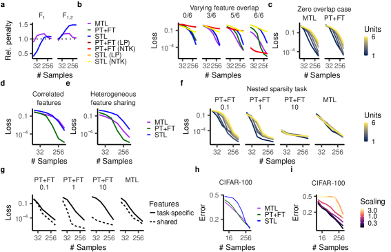
Figure 3: Nonlinear networks. a: $\mathcal{F}_{1}$ and $\mathcal{F}_{1,2}$ penalty for networks trained on main and auxiliary tasks separately (STL, blue) or jointly (MTL, purple) in a case in which the tasks use the same feature sets (6/6 case in panel b). The x-axis is log scaled. b: Generalization loss (log-scaled) for different numbers of overlapping features (out of 6 total) between main and auxilliary tasks. NTK indicates the (lazy) tangent kernel solution. c: Generalization loss as a function of number of main task features (units in teacher network) in tasks where main and auxiliary task features are disjoint. d: Generalization loss in tasks where main-task features are correlated (0.9 cosine similarity of input weights) with corresponding auxiliary task features. e: Generalization loss for an example with both identically shared and correlated features between tasks. f, Generalization loss for PT+FT using different rescalings of network weights following pretraining (0.1, 1, and 10.0), and also for MTL, on tasks in which main task features are a subset of auxiliary task features. Color indicates number of main task features. g: Generalization loss for same strategies as in panel f, on tasks with one main task feature which either is one of the auxiliary task features (“shared”) or is not (“task-specific”). h: Test error on CIFAR-100 experiment as a function of main task samples (log scale on both axes). i: Test error on CIFAR-100 for PT+FT with different weight rescaling values following pretraining.

As we are unable to characterize PT+FT analytically in the nonlinear case, we turn to experiments and assess the extent to which qualitative insights from the linear theory remain applicable. We find that, as in the diagonal linear case, both MTL and PT+FT are able to effectively leverage feature reuse (outperforming single-task learning when tasks share features, Fig. 3b, right panel) and perform effective feature learning of task-specific features (nearly matching rich single-task learning and substantially outperforming lazy single-task learning when task features are not shared, Fig. 3b, left panel). Moreover, as in the linear theory, both effects can be exhibited simultaneously (Fig. 3b, middle panels). We also confirm that, as in the linear setting, task-specific feature learning exhibits a sparsity bias (greater sample efficiency when non-shared main task features are sparse, Fig. 3c).

6.2 PT+FT bias extends to features correlated with auxiliary task features

Interestingly, in cases with shared features between tasks, we find that finetuning can underperform multi-task learning (Fig. 3b), in contrast to the diagonal linear case. We hypothesize that this effect is caused by the fact that during finetuning, hidden units may not only change their magnitudes, but also the directions $\vec{\theta}_{h}$ of their input weights. Thus, in nonlinear networks, PT+FT may not strictly exhibit a bias toward reusing features across tasks, but rather a “softer” bias that also privileges features correlated with (but not identical to) those learned during pretraining. Though we lack an analytical description of this bias, to validate this intuition, we conduct experiments in which the ground-truth auxiliary and main tasks rely on correlated but distinct features. Indeed, we find PT+FT outperforms MTL in this case (Fig. 3d). Thus, PT+FT (compared to MTL) trades off the flexibility to “softly” share features for reduced sample efficiency when such flexibility is not needed.

In realistic settings, the degree of correlation between features across tasks is likely heterogeneous. To simulate such a scenario, we experiment with auxiliary and main tasks with a mixture of identically shared and correlated features. In this setting, we find that MTL outperforms PT+FT for fewer main task samples, while PT+FT outperforms MTL when more samples are available (Fig. 3e). We hypothesize that this effect arises because the flexibility of PT+FT to rotate hidden unit inputs is most detrimental in the few-sample regime where there is insufficient data to identify correct features.

6.3 The nested feature-learning regime

In Section 5.2, we uncovered a “nested feature-learning” regime, obtained at intermediate values of $\frac{|\beta_{d}|}{|\beta_{d}^{aux}|}$ between the rich and lazy regimes, in which PT+FT is biased toward sparse feature learning biased by the features learned during pretraining. To test whether the same phenomenon arises in ReLU networks, we rescale the network weights following pretraining by various factors (which has the effect of scaling $|\beta_{d}^{aux}|$ for all $d$). We evaluate performance on a suite of tasks that vary the number of features in the main task teacher network and whether those features are shared with the auxiliary task. At intermediate rescaling values we confirm the presence of a nested feature learning regime, characterized by a bias toward sparsity among features reused from the auxiliary task (Fig. 3f) and a preference for reusing features over task-specific feature learning (Fig. 3g). Further rescaling in either direction uncovers the initialization-insensitive feature learning regime and the initialization-biased lazy learning regime. We do not observe nested feature learning behavior in MTL. Note that in these experiments, nested feature learning manifests at a rescaling value of $1.0$ (i.e. no rescaling), unlike the diagonal linear case where no rescaling yielded lazy dynamics without a sparsity bias. The fact that the parameter scalings required to observe this behavior differ between the linear and ReLU cases is consistent with observations of Woodworth et al., (2020) that nonlinear networks can exhibit rich/lazy regime dynamics at different initialization scales than diagonal linear networks, depending on width and other factors. Additionally, we note that the absolute scale of $\frac{|\beta_{d}|}{|\beta_{d}^{aux}|}$ is sensitive to the structure of the tasks (the relative number of features used in each, and the magnitude of the outputs). Thus, for different tasks and architectures, different rescaling values may be needed to enter the nested feature learning regime.

7 Practical applications to deep networks and real datasets

Our analysis has focused on shallow networks trained on synthetic tasks. To test the applicability of our insights, we conduct experiments with convolutional networks (ResNet-18) on a vision task (CIFAR-100), using classification of two image categories as the primary task and classification of the other 98 as the auxiliary task (512 auxiliary samples used). As in our experiments above, MTL and PT+FT improve sample efficiency compared to single-task learning (Fig. 3h). Moreover, the results corroborate our findings in Section 6.2 that MTL performs better than PT+FT with fewer main task samples, while the reverse is true with more samples. A similar finding was made in Weller et al., (2022) in natural language processing tasks, suggesting it is a robust phenomenon.

Our findings in Section 5.2 and Section 6.3 indicate that the nested sparsity bias of PT+FT can be exposed or masked by rescaling the network weights following pretraining. Such a bias may be beneficial when the main task depends only on a small subset of features learned during pretraining, as may often be the case in practice (including in our CIFAR setup, where the auxiliary task involves more data classes than the main task). We experiment with rescaling in our CIFAR setup. A priori, the appropriate rescaling factor is not obvious, so we treat it as a hyperparameter. We find that rescaling values less than $1$ substantially improve finetuning performance (Fig. 3i). Rescaling values too low caused optimization difficulties, but conditioned on model trainability, decreasing the rescaling parameter monotonically improved performance. These results suggest that rescaling network weights before finetuning may be a practically useful technique.

8 Conclusion

In this work we have provided a detailed characterization of the inductive biases associated with two common training strategies, MTL and PT+FT, that have received comparatively little theoretical treatment. We find that these biases are nuanced, incentivizing a combination of feature sharing and sparse task-specific feature learning. In the case of PT+FT, we characterized a novel learning regime – the nested feature-learning regime – which encourages sparsity within features inherited from pretraining. This insight motivates simple techniques for improving PT+FT performance by pushing networks into this regime, which shows promising empirical results. We also identified another distinction between PT+FT and MTL – the ability to use “soft” feature sharing – that leads to a tradeoff in their relative performance as a function of dataset size, observed in realistic settings.

More work is needed to test these phenomena in more complex tasks and larger models. There are also promising avenues for extending our theoretical work. First, in this paper we did not analytically describe the dynamics of PT+FT in ReLU networks, but we expect more progress could be made on this front. Second, our diagonal linear theory could be extended to the case of the widely used cross-entropy loss (see Appendix C for comments on this point). Third, we believe it is important to extend this theoretical framework to more complex network architectures. Nevertheless, our present work already provides new and practical insights into the function of auxiliary task learning.

Appendix A Derivation of the norm minimization bias of PT+FT for diagonal linear networks

We provide a derivation of the norm minimization biases of diagonal linear networks; note that the same result is proved in Azulay et al., (2021).

Recall the parameterization of single-output diagonal linear networks $f:\mathbb{R}^{d}\to\mathbb{R}$:

$$f_{w}(\vec{x})=\vec{\beta}(\vec{w})\cdot\vec{x},\qquad\vec{\beta}(\vec{w})\in\mathbb{R}^{D},$$ (3)

$$\beta_{d}(\vec{w}):={w^{(2)}_{+,d}}\circ\ {w^{(1)}_{+,d}}-{w^{(2)}_{-,d}}\circ{w^{(1)}_{-,d}},$$ (4)

where $\circ$ indicates elementwise multiplication.

We proceed by calculating the gradient flow dynamics of the task loss $L$ with respect to the weights $\vec{w}$. We adopt the notation and strategy of Woodworth et al., (2020). Using the notation $\tilde{X}=[X\;\;{-X}]$, we have:

$$\dot{\vec{w}}^{(1)}(t)=\nabla_{\vec{w}^{(1)}(t)}L=\nabla_{\vec{w}^{(1)}(t)}\left(\|\tilde{X}\left(\vec{w}^{(1)}(t)\circ\vec{w}^{(2)}(t)\right)-y\|_{2}^{2}\right)=-2\tilde{X}^{\top}r(t)\circ\vec{w^{(2)}}(t)$$ (5)

$$\dot{\vec{w}}^{(2)}(t)=\nabla_{\vec{w}^{(2)}(t)}L=\nabla_{\vec{w}^{(2)}(t)}\left(\|\tilde{X}\left(\vec{w}^{(1)}(t)\circ\vec{w}^{(2)}(t)\right)-y\|_{2}^{2}\right)=-2\tilde{X}^{\top}r(t)\circ\vec{w^{(1)}}(t)$$ (6)

If we change coordinates and define $\vec{s}=\frac{1}{2}\left({\vec{w}^{(1)}}+{\vec{w}^{(2)}}\right)$ and $\vec{d}=\frac{1}{2}\left({\vec{w}^{(1)}}-{\vec{w}^{(2)}}\right)$ we have:

$$\dot{\vec{s}}(t)=-2\tilde{X}^{\top}r(t)\circ\vec{s}(t),$$ (7)

$$\dot{\vec{d}}(t)=2\tilde{X}^{\top}r(t)\circ\vec{d}(t).$$ (8)

The solutions to these equations are

$$\vec{s}(t)=\vec{s}(0)\circ\exp\left(-2\tilde{X}^{\top}\int_{0}^{t}r(s)ds\right)$$ (10)

$$\vec{d}(t)=\vec{d}(0)\circ\exp\left(2\tilde{X}^{\top}\int_{0}^{t}r(s)ds\right)$$ (11)

We are interested in the form of the solution $\vec{\beta}$:

$$\vec{\beta}_{\vec{w}}(t)=\vec{w_{+}^{(1)}}(t)\vec{w_{+}^{(2)}}(t)-\vec{w_{-}^{(1)}}(t)\vec{w_{-}^{(2)}}(t),$$ (12)

$$=\left((\vec{s_{+}}(t))^{2}-(\vec{d_{+}}(t))^{2}\right)-\left((\vec{s_{-}}(t))^{2}-(\vec{d_{-}}(t))^{2}\right),$$ (13)

$$=\left((\vec{s_{+}}(t))^{2}-(\vec{s_{-}}(t))^{2}\right)-\left((\vec{d_{+}}(t))^{2}-(\vec{d_{-}}(t))^{2}\right).$$ (14)

We now make the assumption that the weights are initialized with $\vec{w}_{+}(0)=\vec{w}_{-}(0)=\vec{w}_{0}$ and define $\vec{s_{0}}=\frac{1}{2}\left(\vec{w_{0}^{(1)}}+\vec{w_{0}^{(2)}}\right)$ and $\vec{d_{0}}=\frac{1}{2}\left(\vec{w_{0}^{(1)}}-\vec{w_{0}^{(2)}}\right)$. Then,

$$\vec{\beta}_{\vec{w}}(t)=2\vec{s_{0}}^{2}\circ\left(\exp\left(-4X^{\top}\int_{0}^{t}r(s)ds\right)-\exp\left(4X^{\top}\int_{0}^{t}r(s)ds\right)\right)$$ (15)

$$-2\vec{d_{0}}^{2}\circ\left(\exp\left(4X^{\top}\int_{0}^{t}r(s)ds\right)-\exp\left(-4X^{\top}\int_{0}^{t}r(s)ds\right)\right)$$ (16)

$$=2(\vec{s_{0}}^{2}+\vec{d_{0}}^{2})\cdot\sinh\left(-4X^{\top}\int_{0}^{t}r(s)ds\right)$$ (17)

$$=\left((\vec{(w_{0}^{(1)}})^{2}+(\vec{(w_{0}^{(2)}})^{2}\right)\cdot\sinh\left(-4X^{\top}\int_{0}^{t}r(s)ds\right)$$ (18)

Now the solution is in the same form equation (17) of in Appendix D of Woodworth et al., (2020), but with the coefficient in front of the $\sinh$ term replaced by $\left((\vec{(w_{0}^{(1)}})^{2}+(\vec{(w_{0}^{(2)}})^{2}\right)$. Following the rest of their argument, it follows that under the assumption that $\vec{\beta}(\infty)$ fits the training data with zero error, among all such solutions, $\vec{\beta}(\infty)$ minimizes the penalty

$$\|\beta_{d}\|_{Q} :=\sum_{d=1}^{D}\left(((w_{0})_{d}^{(1)})^{2}+((w_{0})_{d}^{(2)})^{2}\right)q\left(\frac{2\beta_{d}}{((w_{0})_{d}^{(1)})^{2}+((w_{0})_{d}^{(2)})^{2}}\right),$$ (19)

$$q(z) =2-\sqrt{4+z^{2}}+z\cdot\textrm{arcsinh}(z/2)$$ (20)

If we assume that the initialization of $\vec{w_{0}^{(2)}}$ is a vector with constant entries $\gamma$ and that $\vec{w_{0}^{(1)}}$ the obtained from learning a minimum parameter norm solution to a pretraining task with effective weights $\vec{\beta}^{aux}$, and hence satisfies $(w_{0})_{d}^{(1)}=\sqrt{|\beta_{d}^{aux}|}$, the result in Equation 1 follows.

Appendix B Derivation of the $\ell_{1,2}$ penalty minimization bias of MTL

B.1 Multi-task diagonal linear networks

Diagonal linear networks with $O$ outputs are parameterized as:

$$f_{w}(x)=\vec{\beta}(\vec{w})x,\qquad\vec{\beta}(\vec{w})\in\mathbb{R}^{O\times D},$$ (21)

$$\beta_{o,d}(\vec{w}):=w^{(2)}_{+,o,d}\circ w^{(1)}_{+,d}-w^{(2)}_{-,o,d}\circ w^{(1)}_{-,d}.$$ (22)

where $\circ$ indicates elementwise product. We are interested in how minimizing the total parameter norm

$$\sum_{d=1}^{D}\left((w^{(1)}_{+,d})^{2}+\sum_{o=1}^{O}(w^{(2)}_{+,o,d})^{2}\right)+\left((w^{(1)}_{-,d})^{2}+\sum_{o=1}^{O}(w^{(2)}_{-,o,d})^{2}\right)$$ (23)

maps to minimizing a norm over the solution weights $\vec{\beta}$. First we note that in the minimum parameter norm solution, for a given input dimension $d$, either all its associated $+$ weights or all its associated $-$ weights will be zero. Without loss of generality we may assume that all the $-$ weights are zero. So we are to minimize

$$\sum_{d=1}^{D}\left((w^{(1)}_{+,d})^{2}+\sum_{o=1}^{O}(w^{(2)}_{+,o,d})^{2}\right)$$ (24)

For given solution coefficients $\vec{\beta_{d}}\in\mathbb{R}^{O}$, the value of the input weight $(w^{(1)}_{+,d})^{2}$ is a free parameter $z_{d}^{2}>0$, as we can set $w^{(2)}_{+,o,d}:=\beta_{o,d}/z$. As any value for $z_{d}$ leads to the same function, we choose $z_{d}$ to minimize

$$((w^{(1)}_{+,d})^{2}+\sum_{o=1}^{O}(w^{(2)}_{+,o,d})^{2}=z_{d}^{2}+\|\vec{\beta_{d}}\|_{2}^{2}/z_{d}^{2}.$$ (25)

Setting the derivative to zero implies

$$z_{d}^{2}=\|\vec{\beta_{d}}\|_{2}.$$ (26)

As a result,

$$\sum_{d=1}^{D}\left((w^{(1)}_{+,d})^{2}+\sum_{o=1}^{O}(w^{(2)}_{+,o,d})^{2}\right)=2\sum_{d=1}^{D}\|\vec{\beta_{d}}\|_{2},$$ (27)

where the right-hand side of the equation is the $\ell_{1,2}$ norm.

Note that this implies, as a special case, that the minimum parameter solution to a diagonal linear network with one output minimizes the $\ell_{1}$ norm.

B.2 Multi-task ReLU networks

Multi-task ReLU networks with a shared feature layer and $O$ outputs can be written as

$$f_{w}(x)=\sum_{h=1}^{H}\vec{w^{(2)}_{h}}(\langle\vec{w^{(1)}_{h}},\vec{x}\rangle)_{+}=\sum_{h=1}^{H}\vec{m_{h}}(\langle\vec{\theta_{h}},\vec{x}\rangle)_{+},$$ (28)

$$\vec{m_{h}}=\vec{w^{(2)}_{h}}\|\vec{w^{(1)}_{h}}\|_{2},\vec{\theta_{h}}=\vec{w^{(1)}_{h}}/\|\vec{w^{(1)}_{h}}\|_{2},$$ (29)

where $\vec{w^{(2)}_{h}},\vec{m_{h}}\in\mathbb{R^{O}}$. As above, we are interested in how minimizing the parameter norm $\sum_{h=1}^{H}\|\vec{w^{(1)}_{h}}\|_{2}^{2}+\|\vec{w^{(2)}_{h}}\|_{2}^{2}$ maps to minimizing a norm over the solution weights $\vec{m}$. For a given $\vec{m_{h}}\in\mathbb{R}^{O}$, the norm of the input weight $\|w^{(1)}_{h}\|_{2}$ is a free parameter $z_{h}>0$, as we can set $w_{h}^{(2)}:=m_{h}/z$. As any value for $z_{h}$ leads to the same function, we choose $z_{h}$ so as to minimize

$$\|\vec{w^{(1)}_{h}}\|_{2}^{2}+\|\vec{w^{(2)}_{h}}\|_{2}^{2}=z_{h}^{2}+\|\vec{m_{h}}\|_{2}^{2}/z_{h}^{2}.$$ (30)

Setting the derivative to zero implies

$$z_{h}^{2}=\|\vec{m_{h}}\|_{2}.$$ (31)

As a result,

$$\sum_{h=1}^{H}\|\vec{w_{h}^{(1)}}\|_{2}^{2}+\|\vec{w_{h}^{(2)}}\|_{2}^{2}=2\sum_{h=1}^{H}\|\vec{m_{h}}\|_{2},$$ (32)

where the right-hand side of the equation is the $\ell_{1,2}$ norm.

Appendix C Comments on cross-entropy vs. mean squared error loss

Cross-entropy and mean squared error are among the most common loss functions in machine learning. An important difference between them is that while mean squared error can be minimized to zero exactly by interpolating the data, cross-entropy achieves its minimum asymptotically as the model predictions become inifinitely large (Gunasekar et al.,, 2018). Consequently, while mean squared error is more amenable to an analysis of the full learning trajectory (Braun et al.,, 2022), cross-entropy is often more easily understood in the asymptotic limit of infinite training. For homogeneous networks, it has been shown that crossentropy induces an implicit regularization towards the minimal parameter $\ell_{2}$-norm (Lyu and Li,, 2020; Nacson et al.,, 2019). Because all the networks we consider are homogeneous, by the results of Appendix B, diagonal neural networks trained on multiple tasks with crossentropy loss for infinite time would indeed minimize the $\ell_{1,2}$-norm, and ReLU networks would minimize the $\mathcal{F}_{1,2}$-norm. However, PT+FT networks would minimize the $\ell_{1}$ and $\mathcal{F}_{1}$ norms, respectively, behaving identically to single-task learning. This is because given infinite training time, the behavior of networks trained with cross-entropy loss is in theory independent of initialization. This behavior is quite different from that of networks trained with mean squared error loss at convergence, which is heavily dependent on initialization (indeed, this is the basis of our investigation in this work). However, prior work has shown that given finite training time, networks trained on cross-entropy loss learn solutions that are sensitive to initialization, and indeed there is a correspondence between increasing training time and decreasing initialization scale (incentivizing rich / feature-learning behavior). Thus, we expect our qualitative findings are applicable to the case of networks trained with cross-entropy loss for finite time. Moreover, our results on the effects of rescaling network parameters (e.g. to uncover the nested feature-learning regime) may be able to be replicated in the cross-entropy setting by scaling training time.

References

- Azulay et al., (2021) Azulay, S., Moroshko, E., Nacson, M. S., Woodworth, B. E., Srebro, N., Globerson, A., and Soudry, D. (2021). On the Implicit Bias of Initialization Shape: Beyond Infinitesimal Mirror Descent. In Proceedings of the 38th International Conference on Machine Learning, pages 468–477. PMLR.
- Bach, (2017) Bach, F. (2017). Breaking the curse of dimensionality with convex neural networks. The Journal of Machine Learning Research, 18(1):629–681.
- Bommasani et al., (2022) Bommasani, R., Hudson, D. A., Adeli, E., Altman, R., Arora, S., von Arx, S., Bernstein, M. S., Bohg, J., Bosselut, A., Brunskill, E., Brynjolfsson, E., Buch, S., Card, D., Castellon, R., Chatterji, N., Chen, A., Creel, K., Davis, J. Q., Demszky, D., Donahue, C., Doumbouya, M., Durmus, E., Ermon, S., Etchemendy, J., Ethayarajh, K., Fei-Fei, L., Finn, C., Gale, T., Gillespie, L., Goel, K., Goodman, N., Grossman, S., Guha, N., Hashimoto, T., Henderson, P., Hewitt, J., Ho, D. E., Hong, J., Hsu, K., Huang, J., Icard, T., Jain, S., Jurafsky, D., Kalluri, P., Karamcheti, S., Keeling, G., Khani, F., Khattab, O., Koh, P. W., Krass, M., Krishna, R., Kuditipudi, R., Kumar, A., Ladhak, F., Lee, M., Lee, T., Leskovec, J., Levent, I., Li, X. L., Li, X., Ma, T., Malik, A., Manning, C. D., Mirchandani, S., Mitchell, E., Munyikwa, Z., Nair, S., Narayan, A., Narayanan, D., Newman, B., Nie, A., Niebles, J. C., Nilforoshan, H., Nyarko, J., Ogut, G., Orr, L., Papadimitriou, I., Park, J. S., Piech, C., Portelance, E., Potts, C., Raghunathan, A., Reich, R., Ren, H., Rong, F., Roohani, Y., Ruiz, C., Ryan, J., Ré, C., Sadigh, D., Sagawa, S., Santhanam, K., Shih, A., Srinivasan, K., Tamkin, A., Taori, R., Thomas, A. W., Tramèr, F., Wang, R. E., Wang, W., Wu, B., Wu, J., Wu, Y., Xie, S. M., Yasunaga, M., You, J., Zaharia, M., Zhang, M., Zhang, T., Zhang, X., Zhang, Y., Zheng, L., Zhou, K., and Liang, P. (2022). On the Opportunities and Risks of Foundation Models. arXiv:2108.07258 [cs].
- Boursier et al., (2022) Boursier, E., Pillaud-Vivien, L., and Flammarion, N. (2022). Gradient flow dynamics of shallow ReLU networks for square loss and orthogonal inputs.
- Braun et al., (2022) Braun, L., Dominé, C., Fitzgerald, J., and Saxe, A. (2022). Exact learning dynamics of deep linear networks with prior knowledge. Advances in Neural Information Processing Systems, 35:6615–6629.
- Chizat and Bach, (2020) Chizat, L. and Bach, F. (2020). Implicit Bias of Gradient Descent for Wide Two-layer Neural Networks Trained with the Logistic Loss. In Proceedings of Thirty Third Conference on Learning Theory, pages 1305–1338. PMLR. ISSN: 2640-3498.
- Chizat et al., (2019) Chizat, L., Oyallon, E., and Bach, F. (2019). On Lazy Training in Differentiable Programming. In Advances in Neural Information Processing Systems, volume 32. Curran Associates, Inc.
- Dery et al., (2021) Dery, L. M., Michel, P., Talwalkar, A., and Neubig, G. (2021). Should We Be Pre-training? An Argument for End-task Aware Training as an Alternative.
- Du et al., (2022) Du, Y., Liu, Z., Li, J., and Zhao, W. X. (2022). A Survey of Vision-Language Pre-Trained Models. arXiv:2202.10936 [cs].
- Fort et al., (2020) Fort, S., Dziugaite, G. K., Paul, M., Kharaghani, S., Roy, D. M., and Ganguli, S. (2020). Deep learning versus kernel learning: an empirical study of loss landscape geometry and the time evolution of the Neural Tangent Kernel. In Advances in Neural Information Processing Systems, volume 33, pages 5850–5861. Curran Associates, Inc.
- Gunasekar et al., (2018) Gunasekar, S., Lee, J. D., Soudry, D., and Srebro, N. (2018). Implicit Bias of Gradient Descent on Linear Convolutional Networks. In Advances in Neural Information Processing Systems, volume 31. Curran Associates, Inc.
- HaoChen et al., (2021) HaoChen, J. Z., Wei, C., Lee, J., and Ma, T. (2021). Shape Matters: Understanding the Implicit Bias of the Noise Covariance. In Proceedings of Thirty Fourth Conference on Learning Theory, pages 2315–2357. PMLR.
- Huh et al., (2023) Huh, M., Mobahi, H., Zhang, R., Cheung, B., Agrawal, P., and Isola, P. (2023). The Low-Rank Simplicity Bias in Deep Networks. arXiv:2103.10427 [cs].
- Jacot et al., (2020) Jacot, A., Gabriel, F., and Hongler, C. (2020). Neural Tangent Kernel: Convergence and Generalization in Neural Networks. arXiv:1806.07572 [cs, math, stat].
- Jaderberg et al., (2016) Jaderberg, M., Mnih, V., Czarnecki, W. M., Schaul, T., Leibo, J. Z., Silver, D., and Kavukcuoglu, K. (2016). Reinforcement Learning with Unsupervised Auxiliary Tasks. arXiv:1611.05397 [cs].
- Kornblith et al., (2019) Kornblith, S., Shlens, J., and Le, Q. V. (2019). Do better ImageNet models transfer better?
- Kumar et al., (2022) Kumar, A., Raghunathan, A., Jones, R., Ma, T., and Liang, P. (2022). Fine-Tuning can Distort Pretrained Features and Underperform Out-of-Distribution. arXiv:2202.10054 [cs].
- Lyu and Li, (2020) Lyu, K. and Li, J. (2020). Gradient Descent Maximizes the Margin of Homogeneous Neural Networks. arXiv:1906.05890 [cs, stat].
- Maurer et al., (2016) Maurer, A., Pontil, M., and Romera-Paredes, B. (2016). The Benefit of Multitask Representation Learning. Journal of Machine Learning Research, 17(81):1–32.
- Moroshko et al., (2020) Moroshko, E., Woodworth, B. E., Gunasekar, S., Lee, J. D., Srebro, N., and Soudry, D. (2020). Implicit Bias in Deep Linear Classification: Initialization Scale vs Training Accuracy. In Advances in Neural Information Processing Systems, volume 33, pages 22182–22193. Curran Associates, Inc.
- Mulayoff et al., (2021) Mulayoff, R., Michaeli, T., and Soudry, D. (2021). The Implicit Bias of Minima Stability: A View from Function Space. In Advances in Neural Information Processing Systems, volume 34, pages 17749–17761. Curran Associates, Inc.
- Nacson et al., (2019) Nacson, M. S., Gunasekar, S., Lee, J., Srebro, N., and Soudry, D. (2019). Lexicographic and Depth-Sensitive Margins in Homogeneous and Non-Homogeneous Deep Models. In Proceedings of the 36th International Conference on Machine Learning, pages 4683–4692. PMLR. ISSN: 2640-3498.
- Neyshabur, (2017) Neyshabur, B. (2017). Implicit Regularization in Deep Learning. arXiv:1709.01953 [cs].
- Pesme et al., (2021) Pesme, S., Pillaud-Vivien, L., and Flammarion, N. (2021). Implicit Bias of SGD for Diagonal Linear Networks: a Provable Benefit of Stochasticity.
- Pilanci and Ergen, (2020) Pilanci, M. and Ergen, T. (2020). Neural Networks are Convex Regularizers: Exact Polynomial-time Convex Optimization Formulations for Two-layer Networks. arXiv:2002.10553 [cs, stat].
- Rahaman et al., (2018) Rahaman, N., Baratin, A., Arpit, D., Draxler, F., Lin, M., Hamprecht, F., Bengio, Y., and Courville, A. (2018). On the Spectral Bias of Neural Networks.
- Razin and Cohen, (2020) Razin, N. and Cohen, N. (2020). Implicit Regularization in Deep Learning May Not Be Explainable by Norms. In Advances in Neural Information Processing Systems, volume 33, pages 21174–21187. Curran Associates, Inc.
- Refinetti et al., (2023) Refinetti, M., Ingrosso, A., and Goldt, S. (2023). Neural networks trained with SGD learn distributions of increasing complexity. arXiv:2211.11567 [cond-mat, stat].
- Ruder, (2017) Ruder, S. (2017). An Overview of Multi-Task Learning in Deep Neural Networks. arXiv:1706.05098 [cs, stat].
- Savarese et al., (2019) Savarese, P., Evron, I., Soudry, D., and Srebro, N. (2019). How do infinite width bounded norm networks look in function space?: 32nd Conference on Learning Theory, COLT 2019. Proceedings of Machine Learning Research, 99:2667–2690.
- Saxe et al., (2022) Saxe, A., Sodhani, S., and Lewallen, S. J. (2022). The Neural Race Reduction: Dynamics of Abstraction in Gated Networks. In Proceedings of the 39th International Conference on Machine Learning, pages 19287–19309. PMLR. ISSN: 2640-3498.
- Shachaf et al., (2021) Shachaf, G., Brutzkus, A., and Globerson, A. (2021). A Theoretical Analysis of Fine-tuning with Linear Teachers. In Advances in Neural Information Processing Systems, volume 34, pages 15382–15394. Curran Associates, Inc.
- Steed et al., (2022) Steed, R., Panda, S., Kobren, A., and Wick, M. (2022). Upstream Mitigation Is Not All You Need: Testing the Bias Transfer Hypothesis in Pre-Trained Language Models. In Proceedings of the 60th Annual Meeting of the Association for Computational Linguistics (Volume 1: Long Papers), pages 3524–3542, Dublin, Ireland. Association for Computational Linguistics.
- Vafaeikia et al., (2020) Vafaeikia, P., Namdar, K., and Khalvati, F. (2020). A Brief Review of Deep Multi-task Learning and Auxiliary Task Learning. arXiv:2007.01126 [cs, stat].
- Vyas et al., (2022) Vyas, N., Bansal, Y., and Nakkiran, P. (2022). Limitations of the NTK for Understanding Generalization in Deep Learning. arXiv:2206.10012 [cs].
- Wang and Russakovsky, (2023) Wang, A. and Russakovsky, O. (2023). Overwriting Pretrained Bias with Finetuning Data. arXiv:2303.06167 [cs].
- Wang and Lin, (2021) Wang, H. and Lin, W. (2021). Harmless Overparametrization in Two-layer Neural Networks. arXiv:2106.04795 [cs, math, stat].
- Wang et al., (2022) Wang, Y., Lacotte, J., and Pilanci, M. (2022). The Hidden Convex Optimization Landscape of Two-Layer ReLU Neural Networks: an Exact Characterization of the Optimal Solutions. arXiv:2006.05900 [cs, stat].
- Weller et al., (2022) Weller, O., Seppi, K., and Gardner, M. (2022). When to Use Multi-Task Learning vs Intermediate Fine-Tuning for Pre-Trained Encoder Transfer Learning. In Proceedings of the 60th Annual Meeting of the Association for Computational Linguistics (Volume 2: Short Papers), pages 272–282, Dublin, Ireland. Association for Computational Linguistics.
- Woodworth et al., (2020) Woodworth, B., Gunasekar, S., Lee, J. D., Moroshko, E., Savarese, P., Golan, I., Soudry, D., and Srebro, N. (2020). Kernel and Rich Regimes in Overparametrized Models. In Proceedings of Thirty Third Conference on Learning Theory, pages 3635–3673. PMLR. ISSN: 2640-3498.
- Wu et al., (2020) Wu, S., Zhang, H. R., and Ré, C. (2020). Understanding and Improving Information Transfer in Multi-Task Learning. arXiv:2005.00944 [cs].
- Yang and Hu, (2021) Yang, G. and Hu, E. J. (2021). Tensor Programs IV: Feature Learning in Infinite-Width Neural Networks. In Proceedings of the 38th International Conference on Machine Learning, pages 11727–11737. PMLR.
- Yuan and Lin, (2006) Yuan, M. and Lin, Y. (2006). Model selection and estimation in regression with grouped variables. Journal of the Royal Statistical Society: Series B (Statistical Methodology), 68(1):49–67. _eprint: https://onlinelibrary.wiley.com/doi/pdf/10.1111/j.1467-9868.2005.00532.x.
- Zhang and Yang, (2022) Zhang, Y. and Yang, Q. (2022). A Survey on Multi-Task Learning. IEEE Transactions on Knowledge and Data Engineering, 34(12):5586–5609. Conference Name: IEEE Transactions on Knowledge and Data Engineering.
- Zhou et al., (2023) Zhou, C., Li, Q., Li, C., Yu, J., Liu, Y., Wang, G., Zhang, K., Ji, C., Yan, Q., He, L., Peng, H., Li, J., Wu, J., Liu, Z., Xie, P., Xiong, C., Pei, J., Yu, P. S., and Sun, L. (2023). A Comprehensive Survey on Pretrained Foundation Models: A History from BERT to ChatGPT. arXiv:2302.09419 [cs].