Higher orders for cosmological phase transitions:
A global study in a Yukawa model

Abstract

We perform a state-of-the-art global study of the cosmological thermal histories of a simple Yukawa model, and find higher perturbative orders to be important for determining both the presence and strength of strong first-order phase transitions. Using high-temperature effective field theory, we calculate the free energy density of the model up to $\mathcal{O}(y^{5}T^{4})$, where $y$ is the Yukawa coupling and $T$ is the temperature. The locations of phase transitions are found using the results of lattice Monte-Carlo simulations, and the strength of first-order transitions are evaluated within perturbation theory, to 3-loop order. This is the first global study of any model at this order. Compared to a vanilla 1-loop analysis, accurate to $\mathcal{O}(y^{2}T^{4})$, reaching such accuracy enables on average a five-fold reduction in the relative error in the predicted critical temperature $T_{\text{c}}$, and an additional $\sim 50\%$ strong first-order transitions with latent heat $L/T_{\text{c}}^{4}>0.1$ to be identified in our scan.

1 Introduction

Extensions of the Standard Model (SM) of particle physics can lead to additional phase transitions in the early universe, with consequences for open problems such as baryogensis and dark matter. This in turn can produce a gravitational wave background detectable at current and future detectors such as LISA LISA:2017pwj , Taiji Ruan:2018tsw , TianQin TianQin:2015yph , DECIGO Kawamura:2011zz , NANOGrav NANOGrav:2023hvm and the International Pulsar Timing Array Hobbs:2009yy . For a sizeable gravitational wave background to be produced requires a first-order phase transition, unlike the smooth crossovers corresponding to electroweak symmetry breaking DOnofrio:2015gop and colour confinement Aoki:2006we in the SM.

We study perhaps the simplest model giving rise to a first-order phase transition, by coupling a real scalar field ($\phi$) to a Dirac fermion ($\psi$) via a Yukawa interaction,

$$\mathscr{L}=\mathscr{L}_{\text{Scalar}}+\mathscr{L}_{\text{Dirac}}+\mathscr{L}_{\text{Yukawa}}\ ,$$ (1)

where, in the mostly minus metric and using the Feynman slash notation, $\not{\partial}=\gamma^{\mu}\partial_{\mu}$,

$$\mathscr{L}_{\text{Scalar}} =\frac{1}{2}\partial_{\mu}\phi\partial^{\mu}\phi-\sigma\phi-\frac{1}{2}m^{2}\phi^{2}-\frac{1}{3!}g\phi^{3}-\frac{1}{4!}\lambda\phi^{4},$$ (2)

$$\mathscr{L}_{\text{Dirac}} =\bar{\psi}(i\not{\partial}-m_{\psi})\psi,$$ (3)

$$\mathscr{L}_{\text{Yukawa}} =-y\phi\bar{\psi}\psi.$$ (4)

In principle, this Yukawa theory may be coupled to the SM through the Higgs portal. The resulting model has been widely studied as providing a simple dark matter candidate Kim:2008pp ; Baek:2011aa ; Baek:2012uj ; Esch:2013rta ; Buchmueller:2013dya ; Klasen:2013ypa ; Esch:2014jpa ; Freitas:2015hsa ; Baek:2015lna ; Dupuis:2016fda ; Albert:2016osu ; Bell:2016ekl , and is sometimes known as singlet fermionic dark matter. Phase transitions in this model have been studied in refs. Fairbairn:2013uta ; Li:2014wia ; Beniwal:2018hyi . However, in what follows, we will neglect Higgs portal couplings, and focus on the minimal model of $\phi$ and $\psi$, as our primary interest is the reliability and convergence of perturbative approaches to first-order phase transitions. Our model can still have more direct physical relevance in the context of feebly interacting massive particles Bernal:2017kxu ; Yaguna:2023kyu .

At the high temperatures necessary for a phase transition, with $\pi T$ large compared to $m$ and $m_{\psi}$, the usual loop expansion breaks down due to the hierarchy of scales introduced between the temperature and relevant masses. Whereas the mass of the zero Matsubara mode has thermal contributions only at the soft scale $\mathcal{O}(yT)$, the nonzero Matsubara modes receive thermal contributions to their masses at the hard scale $\mathcal{O}(\pi T)$. This scale hierarchy causes some Feynman diagrams to be larger than suggested by loop counting. Effective field theory, applied in the framework of high-temperature dimensional reduction Farakos:1994kx ; Farakos:1994xh ; Braaten:1995cm ; Kajantie:1995dw ; Braaten:1995jr , offers a systematic means to account for this through resummations, and the only framework which has been pushed to higher perturbative orders. For an introduction, see ref. Braaten:1995cm .

Perturbative calculations of the thermodynamics of cosmological phase transitions have been observed to suffer from huge theoretical uncertainties in a variety of models, often amounting to a factor of between a hundred and a million for the predicted gravitational wave peak amplitude. Numerically, often the largest theoretical uncertainty appears as a strong dependence of physical observables on the renormalisation scale Croon:2020cgk ; Papaefstathiou:2020iag ; Gould:2021oba ; Athron:2022jyi ; Curtin:2022ovx ; Kierkla:2022odc . Relatedly, computations using different approximations have been found to yield drastically different predictions Carena:2019une ; Ellis:2022lft . However, this uncertainty is significantly reduced with higher order dimensional reduction, demonstrating the importance of such calculations.

High-temperature dimensional reduction has been applied at 2-loop order to a wide range of models, including the Standard Model Kajantie:1995dw and a number of its extensions (see for example refs. Gorda:2018hvi ; Biondini:2022ggt ), and at 3-loop and partial 4-loop order to QCD Braaten:1995jr ; Kajantie:2002wa and the Standard Model in the electroweak symmetric phase Gynther:2005dj . The generic rules of dimensional reduction were put down in ref. Kajantie:1995dw , and the first software package to carry this out, DRalgo, was published recently Ekstedt:2022bff . The dimensional reduction of the Yukawa model considered here has not previously been carried out. Our results in fact provided a correction for DRalgo, to be included in an upcoming release.

Motivated by making reliable predictions for gravitational wave experiments, recently there has been growing interest in quantifying and reducing theoretical uncertainties for cosmological phase transitions Cutting:2019zws ; Giese:2020znk ; Croon:2020cgk ; Jinno:2020eqg ; Ajmi:2022nmq ; Athron:2022jyi ; Sagunski:2023ynd ; Athron:2023rfq . A number of recent studies have tested the validity and accuracy of perturbation theory, utilising dimensional reduction to push to higher orders Kainulainen:2019kyp ; Croon:2020cgk ; Niemi:2020hto ; Niemi:2021qvp ; Gould:2021oba ; Tenkanen:2022tly ; Gould:2023ovu . While these studies showed that lower-order calculations can suffer from large theoretical uncertainties, this was based on studying a small number of benchmark parameter points. One is led to wonder how generic these conclusions are. For example, in a broad scan of the parameter space of a model, do the global features of the results change between successive perturbative orders; in short, does the blob move? In this work, we aim to address this and related questions for our Yukawa model.

2 Dimensional reduction

Equilibrium thermodynamics of quantum field theories can be studied in the imaginary time formalism Kapusta:2006pm . The fields of the partition function are defined in three infinite spatial directions and one compact direction with length $1/T$. In the compact direction, bosons, including the scalar $\phi$ in our model, satisfy periodic boundary conditions and can be expanded as

$$\phi(\tau,\mathbf{x})={{\sum}}_{n=-\infty}^{\infty}\varphi_{n}(\mathbf{x})e^{i2n\pi T\tau}\ ,$$ (5)

where $\tau$ parameterise the compact direction and $\mathbf{x}$ the spatial directions. On the other hand, fermions such as $\psi$ satisfy anti-periodic boundary conditions and can be expanded as

$$\psi(\tau,\mathbf{x})={{\sum}}_{n=-\infty}^{\infty}\uppsi_{n}(\mathbf{x})e^{i(2n+1)\pi T\tau}\ .$$ (6)

These Fourier modes are referred to as Matsubara modes Matsubara:1955ws . The free part of the Euclidean equilibrium action can be written as

$$S_{0}=\frac{1}{T}\int d^{3}\mathbf{x}{{\sum}}_{n=-\infty}^{\infty}\bigg{[} \frac{1}{2}(\partial_{i}\varphi_{n})^{2}+\frac{1}{2}(2\pi Tn)^{2}\varphi_{n}^{2}+\frac{1}{2}m^{2}\varphi_{n}^{2}$$

$$+\bar{\uppsi}_{n}\left(\gamma_{i}\partial_{i}+i2\pi T(n+1)\gamma_{0}+m_{\psi}\right)\uppsi_{n}\bigg{]}\ ,$$ (7)

where $\gamma_{i}$ and $\gamma_{0}$ are Euclidean gamma matrices Laine:2016hma .

Thus one can view the equilibrium thermodynamics of the four dimensional (4d) theory as the vacuum dynamics of infinitely many 3d fields Andersen:2004fp , the fields $\varphi_{n}$ with effective squared masses $m_{n}^{2}=m^{2}+(2\pi Tn)^{2}$  and the fields $\uppsi_{n}$ with effective squared masses $m_{\psi}^{2}+(2\pi T(n+1))^{2}$.

At temperature $T$ the effective coupling constant of the $n=0$ light bosonic mode increases as $\propto T/m_{0}$, reflecting its high occupancy $n_{\text{B}}\sim T/m_{0}$. The naive perturbative expansion for this mode therefore breaks down at high temperatures. A resummed perturbative expansion is nevertheless possible, though its convergence is slower than at zero temperature.

At high temperatures some form of resummation is necessary, yet the specifics depend on what assumptions are made regarding the relative magnitudes of different parameters Lofgren:2023sep . In this paper, the following power counting prescriptions were adopted for the parameters of the Yukawa theory, fixing the relative sizes of the couplings such that: (i) the loop expansion parameters at zero temperature are of similar size, and (ii) the thermal contributions to the effective potential are of similar size to the tree-level terms, as expected for a phase transition (additional details given in appendix A):

$$\frac{\sigma}{T^{3}}\sim\frac{m^{2}}{T^{2}}\sim\frac{g}{T}\sim\lambda\sim y^{2}\sim\frac{m_{\psi}^{2}}{T^{2}}\ .$$ (8)

Using the hierarchy of scales between masses and the temperature, we can construct an effective field theory (EFT) for only the light modes. This construction is referred to as dimensional reduction due to the EFT being defined in three dimensions, and is the most general 3d theory obeying the same internal and spatial symmetries as the 4d theory, as well as having the same number of light bosonic degrees of freedom:

$$\mathscr{L}_{\text{3}} =\frac{1}{2}(\partial_{i}\phi_{3})^{2}+\sigma_{3}\phi_{3}+\frac{1}{2}m_{3}^{2}\phi_{3}^{2}+\frac{1}{3!}g_{3}\phi_{3}^{3}+\frac{1}{4!}\lambda_{3}\phi_{3}^{4}\ .$$ (9)

In principle, higher dimensional operators could be added to this effective Lagrangian, though these turn up at one higher order in $y$ than we work, using the power counting prescription of equation (8) Braaten:1995cm ; Niemi:2021qvp .

At a first-order phase transition, the different terms in equation (9) balance to yield two minima with a maximum between. For this to be possible, the different terms in the potential must be the same order of magnitude, such as $m_{3}^{2}\phi_{3}^{2}\sim\lambda_{3}\phi_{3}^{4}$. Extending the power counting to the 3d couplings, $m_{3}^{2}\sim m^{2}\sim y^{2}T^{2}$ and $\lambda_{3}\sim\lambda T\sim y^{2}T$, this relation leads to

$$\Rightarrow\phi_{3}^{2} \sim T\,,$$ (10)

so that relatively strong phase transitions are possible in this model. Note that the powers of temperature arise through first scaling the 3d scalar field to canonically normalise it, and then absorbing all explicit factors of $T$ into the parameters of the EFT Braaten:1995cm ; Kajantie:1995dw .

At high temperatures and at leading order (LO), the free energy density of the Yukawa theory is $f=-\pi^{2}T^{4}/20$, independently of the background scalar field. For first-order phase transitions, it is the difference between phases $\Delta f$ which determines the dynamics. For homogeneous phases, the free energy density is equal to the thermal effective potential, and its expansion takes the form

$$\frac{\Delta f}{T^{4}} =\underbrace{c_{2}y^{2}}_{\textup{1-loop}}+\underbrace{c_{3}y^{3}}_{\textup{1-loop}^{+}}+\underbrace{c_{4}y^{4}}_{\textup{2-loop}^{+}}+\underbrace{c_{5}y^{5}}_{\textup{3-loop}^{+}}+\underbrace{c_{6}y^{6}}_{\textup{4-loop}^{+}}+\dots$$ (11)

where the superscript ⁺ indicates that these terms require resummation to compute. The coefficients $c_{n}$ are all of $\mathcal{O}(1)$ in our power counting, and are temperature dependent. In this work, we have evaluated the free energy density up to the $\mathcal{O}({y^{5}T^{4}})$ term, i.e. calculating up to $c_{5}$. This is then compared to the result at leading order, with the free energy density at $\mathcal{O}({y^{2}T^{4}})$, i.e. just $c_{2}$. For brevity, we will refer to results using the full calculation as $\mathcal{O}({y^{5}})$ and leading order results as $\mathcal{O}({y^{2}})$.

Loops of the hard energy scale $\pi T$ (i.e. the dimensional reduction) yield an expansion in integer powers of $y^{2}$. The half-integer powers come from loops within the soft scale EFT, where the energy scale is $yT$ (or $\sqrt{\lambda}T$). The expansion parameter for the soft scale is $\alpha_{3}\sim y$; see equation (38).

To derive the effective couplings of the EFT, we matched the off-shell correlation functions at soft external momenta: zero Matsubara modes with $p\sim yT$. We evaluated the connected, one-particle irreducible correlation functions, denoted by $\Gamma^{(k)}$ in the 4d theory and $\Gamma_{3}^{(k)}$ in the 3d effective theory. The calculations yield generic soft-scale observables accurate up to the $\mathcal{O}({y^{5}T^{4}})$ term for the free energy density. These are given in appendix B. By matching these physical observables, we arrive at expressions for the 3d effective parameters:

$$\begin{split}\phi_{3}^{2}={}&\frac{\bar{\varphi}_{0}^{2}}{T}\left(1+\frac{4y^{2}}{3(4\pi)^{2}}\right)\end{split}$$ (12)

$$\begin{split}\sigma_{3}={}&\left(\frac{\bar{\sigma}}{\sqrt{T}}+\frac{\bar{g}T^{\frac{3}{2}}}{24}+\frac{\bar{y}\bar{m}_{\psi}T^{\frac{3}{2}}}{6}\right)\left(1-\frac{2y^{2}}{3(4\pi)^{2}}\right)+\frac{g\lambda T^{\frac{3}{2}}}{6(4\pi)^{2}}\left[\log\left(\frac{\Lambda}{3T}\right)-c\right]+\frac{y^{2}gT^{\frac{3}{2}}\log 2}{2(4\pi)^{2}}\end{split}$$ (13)

$$\begin{split}m^{2}_{3}={}&\left(\bar{m}^{2}+\frac{\bar{\lambda}T^{2}}{24}+\frac{\bar{y}^{2}T^{2}}{6}\right)\left(1-\frac{4y^{2}}{3(4\pi)^{2}}\right)+\frac{\lambda^{2}T^{2}}{6(4\pi)^{2}}\left[\log\left(\frac{\Lambda}{3T}\right)-c\right]+\frac{y^{2}\lambda T^{2}\log 2}{2(4\pi)^{2}}\end{split}$$ (14)

$$\begin{split}g_{3}={}&\sqrt{T}\bar{g}\left(1-\frac{2y^{2}}{(4\pi)^{2}}\right)\end{split}$$ (15)

$$\begin{split}\lambda_{3}={}&T\bar{\lambda}\left(1-\frac{8y^{2}}{3(4\pi)^{2}}\right)\ ,\end{split}$$ (16)

where couplings either do not have running at $\mathcal{O}({y^{4}})$, or are barred couplings defined to make transparent the renormalisation scale invariance at $\mathcal{O}({y^{4}})$:

$$\bar{\chi}={} \chi-\frac{1}{2}\beta_{\chi}^{\text{b}}L_{b}(\Lambda)-\frac{1}{2}\beta_{\chi}^{\text{f}}L_{f}(\Lambda)$$ (17)

where $\beta_{\chi}=\beta_{\chi}^{\text{b}}+\beta_{\chi}^{\text{f}}$ denotes the beta functions, given in appendix D, $L_{b}(\Lambda)$ and $L_{f}(\Lambda)$ are logarithms of the renormalisation scale, defined following ref. Kajantie:1995dw and given in appendix B, $\gamma_{E}$ is the Euler–Mascheroni constant, and c is a constant arising from 2-loop sum-integrals, also given in appendix B. Similarly to the barred couplings, we defined:

$$\bar{\varphi}_{0}=\varphi_{0}-\frac{1}{2}\gamma_{\phi}\varphi_{0}L_{f}(\Lambda)\ ,$$ (18)

where $\gamma_{\phi}=-\frac{1}{\varphi_{0}}d\varphi_{0}/d(\log\Lambda)=-2y^{2}/(4\pi)^{2}$. All couplings and fields here are $\overline{\text{MS}}$ renormalised. These dimensional reduction relations extend the leading-order results of ref. Gould:2021ccf .

These expressions for the 3d effective parameters now enable perturbative analysis of the EFT to yield results applicable to the 4d Yukawa model. The scale $\Lambda$ can be replaced with two separate renormalisation scales, $\mu$ and $\mu_{3}$ which may be chosen independently Kajantie:1995dw . The $\Lambda$ scales explicitly shown in equations (13) and (14) reproduce the renormalisation group running of the 3d EFT, allowing us to exchange for some new scale $\mu_{3}$ that can be chosen independently. Given the superrenormalisability of the 3d EFT, this running can be upgraded to be exact by replacing $g\lambda T^{3/2}\to g_{3}\lambda_{3}$ and $\lambda^{2}T^{2}\to\lambda_{3}^{2}$ in front of the logarithms of $\Lambda$ in equations (13) and (14). The remaining $\Lambda$ scale dependence carried implicitly in the 4d $\overline{\text{MS}}$ parameters is then denoted as $\mu$ for clarity.

3 Phase transitions and latent heat

3.1 Conditions for first-order phase transition

The pattern of phase transitions in this 3d EFT has been studied in ref. Gould:2021dzl . The existence and order of any phase transitions can be determined as follows. One can find a basis in which $g_{3}(T)=0$ for all $T$ by shifting $\phi_{3}\rightarrow\phi_{3}-g_{3}/\lambda_{3}$. The bare potential then takes the following form:

$$V=\tilde{\sigma}_{3}\phi_{3}+\frac{1}{2}(\tilde{m}_{3}^{2}+\delta m_{3}^{2})\phi_{3}^{2}+\frac{1}{4!}\lambda_{3}\phi_{3}^{4}\ ,$$ (19)

where we have defined

$$\tilde{\sigma}_{3} =\sigma_{3}+\frac{g_{3}^{3}}{3\lambda_{3}^{2}}-\frac{g_{3}m_{3}^{2}}{\lambda_{3}}\ , \tilde{m}_{3}^{2} =m_{3}^{2}-\frac{g_{3}^{2}}{2\lambda_{3}}\ .$$ (20)

The mass counterterm is given in equation 59, and the possible tadpole counterterm cancels. This reduces the theory to the $Z_{2}$-symmetric $\phi_{3}^{4}$ theory coupled to a finite $Z_{2}$-breaking external field $\tilde{\sigma}_{3}(T)$. A phase transition, if it exists, occurs at

$$\tilde{\sigma}_{3}(T_{\text{c}})=0\ ,$$ (21)

where the symmetry is restored. This defines the critical temperature, $T_{\text{c}}$. As a consequence of equation (21), the properties of the phase transition, such as its order and strength, may depend only on $\tilde{m}_{3}^{2}$ and $\lambda_{3}$. Further, by dimensional analysis, there can only be non-trivial dependence on the dimensionless ratio $\tilde{m}_{3}^{2}/\lambda_{3}^{2}$. Using mean field theory, one can see that for $\tilde{m}_{3}^{2}/\lambda_{3}^{2}\ll-1$ there is a first-order phase transition, and for $\tilde{m}_{3}^{2}/\lambda_{3}^{2}\gg 1$ there is a crossover. In between, the line of first-order phase transitions ends in a second-order phase transition at $\tilde{m}_{3}^{2}=\tilde{m}_{3,*}^{2}$. The value of $\tilde{m}_{3,*}^{2}$ has been determined using lattice Monte-Carlo simulations to be Sun:2002cc ; Gould:2021dzl

$$\tilde{m}_{3,*}^{2}=\left[0.0015249(48)+\frac{1}{6(4\pi)^{2}}\log\left(\frac{3\mu_{3}}{\lambda_{3}}\right)\right]\lambda_{3}^{2}\ ,$$ (22)

with the number in parenthesis being the statistical uncertainty in the last digits, and the whole expression is evaluated at the critical temperature.

Due to the $Z_{2}$ symmetry at the critical temperature, $\phi_{3}\to-\phi_{3}$, the condition $\tilde{\sigma}_{3}=0$ is exact, and is unmodified by loop corrections within the 3d EFT which can yield odd powers of $y$. Therefore, the perturbative expansion of $T_{\text{c}}$ is one in powers of $y^{2}$, all odd powers of $y$ cancelling due to the symmetry,

$$T_{\text{c}}=T_{\text{c}}^{(0)}(1+a_{2}y^{2}+a_{4}y^{4}+\dots).$$ (23)

The power counting of other couplings and parameters are related to $y$ using the prescription of equation (8). The LO result $T_{\text{c}}^{(0)}$ can be computed with an unresummed 1-loop calculation, while the next-to-leading order correction $a_{2}$ requires 2-loop dimensional reduction to be carried out with the free energy evaluated to at least $\mathcal{O}({y^{4}T^{4}})$. The coefficients $a_{n}$ can be obtained analytically by solving equation (21) in a strict expansion in powers of $y$.

The order of the transition is determined by the sign of $\tilde{m}_{3}^{2}-\tilde{m}_{3,*}^{2}$ at the critical temperature. $\tilde{m}_{3}^{2}$ is determined by purely hard-scale physics and $\tilde{m}_{3,*}^{2}$ is determined by purely soft-scale physics. However, the soft physics is known from lattice simulations, so the only remaining uncertainties in $\tilde{m}_{3}^{2}-\tilde{m}_{3,*}^{2}$ come from the hard scale.

3.2 Phase transitions for Yukawa theory

For a given parameter point in our Yukawa model, the critical temperature (if it exists) and the order of any phase transition can be determined by combining equations (21) and (22) with the expressions for the 3d effective parameters, equations (12) to (16).

Using the dimensional reduction relations at leading order, equation (21) for the critical temperature has a simple analytic solution, about which subleading corrections can be obtained by a strict perturbative expansion. Our higher order results include the subleading term suppressed relatively by $y^{2}$; see equation (23). In what follows, we give explicit analytic results for the critical temperature to this order.

To simplify the results, we introduce 4d tilded parameters, defined in analogy with those in 3d by transforming $\phi\to\phi-g/\lambda$ to eliminate the cubic scalar term. In terms of the (untilded) parameters of the original basis, the (tilded) parameters of the new basis read

$$\tilde{\sigma} =\sigma-\frac{gm^{2}}{\lambda}+\frac{g^{3}}{3\lambda^{2}}, \tilde{m}^{2} =m^{2}-\frac{g^{2}}{2\lambda}, \tilde{g} =0, \tilde{m}_{\psi} =m_{\psi}-\frac{gy}{\lambda},$$ (24)

and $y$ and $\lambda$ are unchanged.

The coefficient of the symmetry-breaking term in the 3d EFT then reads

$$\tilde{\sigma}_{3}(T)=\frac{1}{\sqrt{T}}\bigg{\{} \tilde{\sigma}+\frac{1}{6}y\tilde{m}_{\psi}T^{2}+\frac{1}{(4\pi)^{2}}\bigg{[}4y\tilde{m}_{\psi}^{3}L_{f}-y^{2}\tilde{\sigma}\left(L_{f}+\frac{2}{3}\right)-\frac{24y^{3}\tilde{m}^{2}\tilde{m}_{\psi}}{\lambda}L_{f}$$

$$\qquad+\left(y^{3}\tilde{m}_{\psi}\left(\frac{1}{3}L_{b}-L_{f}-\frac{1}{9}\right)-\frac{4y^{5}\tilde{m}_{\psi}}{\lambda}L_{f}\right)T^{2}\bigg{]}+\mathcal{O}(y^{4}\tilde{\sigma})\bigg{\}}.$$ (25)

Solving $\tilde{\sigma}_{3}(T_{\text{c}})=0$ in a strict expansion, using the free energy to $\mathcal{O}({y^{5}T^{4}})$, we find the critical temperature,

$$T_{\text{c}}^{2}=-\frac{6\tilde{\sigma}}{y\tilde{m}_{\psi}}\left[1+\frac{1}{(4\pi)^{2}}\left(\frac{4y\tilde{m}_{\psi}^{3}}{\tilde{\sigma}}L_{f}+y^{2}(5L_{f}-2L_{b})+\frac{24y^{4}}{\lambda}\left(1-\frac{\tilde{m}^{2}\tilde{m}_{\psi}}{y\tilde{\sigma}}\right)L_{f}\right)+\mathcal{O}(y^{4})\right].$$ (26)

At leading order, this can be expressed in terms of the original 4d parameters as

$$T_{\text{c}}^{(0)}=\sqrt{\frac{2(g^{3}-3g\lambda m^{2}+3\lambda^{2}\sigma)}{y\lambda\left(yg-\lambda m_{\psi}\right)}}\ .$$ (27)

For $y=0$, the scalar and fermion decouple, and $\sqrt{T}\tilde{\sigma}_{3}$ becomes independent of $T$ for any choice $\mu\propto T$, so $\tilde{\sigma}_{3}$ cannot change sign for the scalar-only theory, at least up to this order. As a consequence the only possible phase transition for the scalar-only theory is of second order, where $\tilde{\sigma}_{3}=0$ for all temperatures and the transition takes place when $\tilde{m}_{3}^{2}-\tilde{m}_{3,*}^{2}$ goes through zero Sun:2002cc . Similarly, $\tilde{\sigma}_{3}$ cannot change sign in the $Z_{2}$ limit of this model, where $\tilde{\sigma}=\tilde{m}_{\psi}=0$, but $y\neq 0$.

If $T_{\text{c}}^{2}$ is negative, then there is no phase transition. If it is positive, equations (20) and (22) can be used to determine $\tilde{m}_{3}^{2}-\tilde{m}_{3,*}^{2}$ and hence the order of the phase transition. The 3d effective mass parameter has a perturbative expansion in integer powers of $y^{2}$, which, when evaluated at the critical temperature, reads

$$\tilde{m}_{3}^{2} =\tilde{m}^{2}-\frac{\tilde{\sigma}}{4y\tilde{m}_{\psi}}\left(\lambda+4y^{2}\right)+\frac{1}{(4\pi)^{2}}\bigg{\{}-\frac{4}{3}y^{2}\tilde{m}^{2}-\frac{1}{2}\lambda\tilde{m}^{2}L_{b}+\left(4y^{2}+24\frac{y^{4}}{\lambda}\right)\tilde{m}^{2}L_{f}$$

$$\qquad\qquad+\left(8y^{2}-\lambda\right)\tilde{m}_{\psi}^{2}L_{f}+\frac{\tilde{\sigma}}{y\tilde{m}_{\psi}}\bigg{[}\frac{4}{3}y^{4}+\left(\frac{1}{3}-3\log 2\right)\lambda y^{2}+\left(\frac{3}{8}\lambda^{2}+\frac{1}{2}\lambda y^{2}\right)L_{b}$$

$$\qquad\qquad\qquad-\left(\frac{1}{4}\lambda y^{2}+10y^{4}+24\frac{y^{6}}{\lambda}\right)L_{f}-\lambda^{2}\left(\log\left(\frac{B}{3}\right)-c\right)\bigg{]}\bigg{\}}+\mathcal{O}(\tilde{m}^{2}y^{4})\,,$$ (28)

where we have chosen both renormalisation scales proportional to the temperature, with $\mu=A\pi T$, and $\mu_{3}=BT$.

Renormalisation scale dependence can be used to estimate the size of missing higher order terms, and so to give an intrinsic measure of the theoretical uncertainty in a prediction. In a strict expansion of a physical quantity, any renormalisation scale dependence cancels exactly, order by order. However, by solving for the running of the parameters to a higher order than the underlying calculation, a formally higher order renormalisation scale dependence can be introduced.

In practice, we have solved the 1-loop renormalisation group equations perturbatively, working to one higher order than the thermodynamic calculation; see appendix D for the beta functions. That is, denoting a 4d $\overline{\text{MS}}$ parameter by $\kappa$, we have solved for the running up to and including the $\mathcal{O}(\kappa y^{2})$ term for our LO thermodynamics, and up to the $\mathcal{O}(\kappa y^{4})$ term for our higher order thermodynamics. As before, $y$ here is used as a shorthand to include terms of equivalent sizes according to the power counting scheme in equation (8). Writing a given $\overline{\text{MS}}$ parameter $\kappa$ as a function of $t=\log\left(\mu^{\prime}/\mu\right)$, the higher order perturbative solution to the running is

$$\kappa(t)\approx\kappa(0)+\beta_{\kappa}(0)t+\frac{1}{2}\sum_{a}\frac{\partial\beta_{\kappa}(0)}{\partial\kappa_{a}(0)}\beta_{\kappa_{a}}(0)t^{2},$$ (29)

where $\kappa_{a}$ runs over all the parameters in the model. Note that while 2-loop contributions to the beta functions would contribute at $\mathcal{O}(\kappa y^{4})$, we do not include them, as we are merely using the running to estimate uncertainties. These running couplings were then included in expressions for the thermodynamic quantities, such as eqs. (26) and (3.2). By then varying the renormalisation scale over a range, we can obtain a measure of the intrinsic uncertainty of the predictions. We chose the renormalisation scales as $\mu=A\pi T_{\text{c}}$, where $A$ varies over 7 equidistant values from $1/2$ to $2$. This range follows standard practice in the field Laine:2017hdk ; Gould:2021oba . The arithmetic mean of the results is taken as the predicted physical quantity, and the minimum and maximum values yield the range of uncertainty. For simplicity, we fix $B=1$ throughout.

3.3 Scan of parameter space

A global study of the parameter space was carried out. Without loss of generality, units were chosen such that $m^{2}=1$, and $\sigma$ was set to zero (this can be fixed by a shift $\phi\to\phi+\text{constant}$). The distributions of the other parameters $y^{2},g^{2},\lambda\text{ and }m_{\psi}$ were chosen according to

$$y^{2},\ \lambda,\ g^{2} \in 10^{\mathcal{U}(-2,~{}0.5)}, m_{\psi} \in\mathcal{U}(0,3),$$ (30)

where $\mathcal{U}(a,b)$ is the uniform distribution on the interval $[a,b)$, and the signs of $y$ and $g$ were chosen randomly and with equal probability. Perturbativity at zero temperature requires that all three couplings are small compared with $\sim 8\pi$ (see e.g. Allwicher:2021rtd ), hence the maximum of the range, and a log distribution was chosen to explore a wide range of possible ratios of couplings. A linear distribution was chosen for the fermion mass parameter because the boundaries between different behaviours occur at $\mathcal{O}(1)$ values of $m_{\psi}$, and no special behaviours are expected (or observed) in the $m_{\psi}\to 0$ limit. Further, large values of $m_{\psi}$ are more likely to invalidate our high-temperature approximation.

If treated as physical parameters, to be consistent with the accuracy of the rest of our calculations, the values generated should be matched to $\overline{\text{MS}}$ parameters at zero temperature at 1-loop order Kajantie:1995dw . However, as we are primarily interested in the perturbative convergence of thermodynamic predictions, rather than interpreting the predictions in a cosmological context, we neglect this zero-temperature matching between $\overline{\text{MS}}$ and physical parameters, instead treating this as a toy model. We therefore carry out a different scan, directly over $\overline{\text{MS}}$ parameter space at the input renormalisation scale $\mu_{0}=1$, carrying over their values directly to the phase transition evaluation.

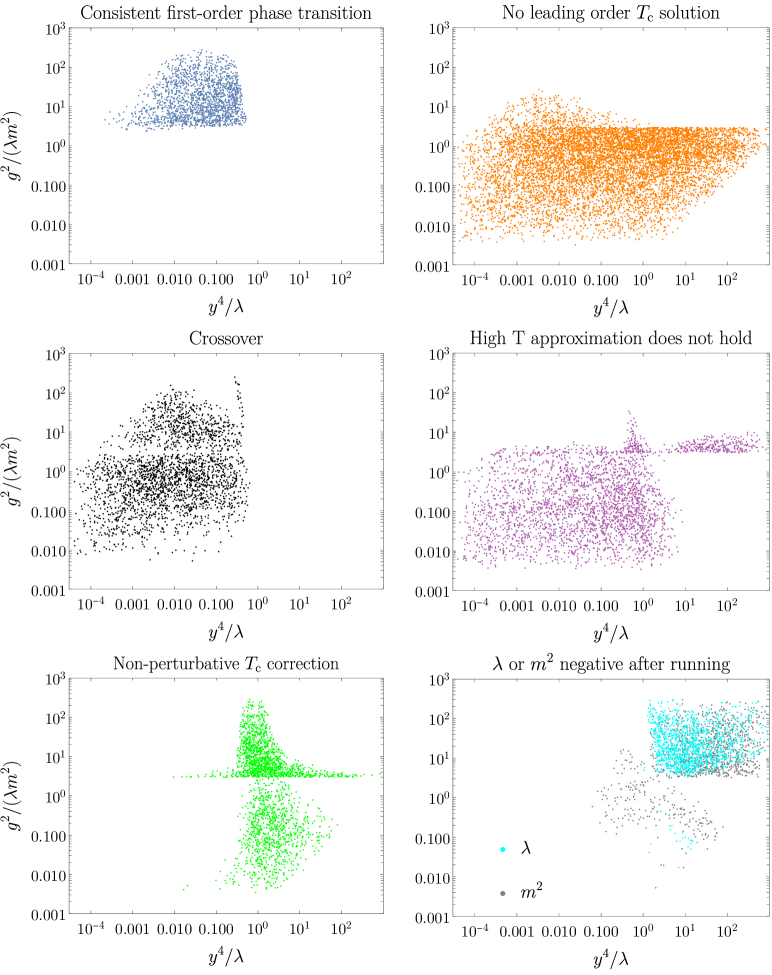
Figure 1: Predicted nature of scalar singlet Yukawa theories studied with free energy evaluated to $\mathcal{O}({y^{5}T^{4}})$ for our scan of parameters. First-order phase transitions were found to be restricted to parameter space where $\frac{g^{2}}{\lambda m^{2}}\gtrsim 2$ and $\frac{y^{4}}{\lambda}\lesssim 0.5$. There are two additional directions in parameter space not shown here, $\lambda$ and $m_{\psi}/m$.

Fig. 1 shows the phase transition evaluation of the Yukawa theory, using the full $\mathcal{O}({y^{5}})$ calculation as per equation (11), for a scan of 20,000 parameter points using the distributions summarised above. The axes are chosen as combinations of parameters which bound the first-order phase transitions identified. We find that first-order phase transitions are limited to parameter space where $\frac{g^{2}}{\lambda}\gtrsim 2m^{2}$. At leading order, this condition follows from the requirement $\tilde{m}_{3}^{2}-\tilde{m}_{3,*}^{2}<0$ for first-order phase transitions, which can be written as

$$\frac{g^{2}}{2\lambda}>m^{2}+\frac{1}{24}(\lambda+4y^{2})T_{\text{c}}^{2}\ ,$$ (31)

with the second term positive definite.

Parameter points are also shown which have no leading order solution for the critical temperature (in orange), or are predicted to be crossovers (in black). Following this are parameter points, shown in purple, where the high temperature approximation does not hold, defined as $T_{\text{c}}<2\cdot\text{max}(m,m_{\psi})$. This precise condition is motivated by the convergence of the high-temperature expansion for the 1-loop thermal functions Laine:2016hma .

It can also be seen from fig. 1 that for values of $\frac{y^{4}}{\lambda}\gtrsim 0.5$, our power counting assumptions can begin to break down. For the points in green, the correction to the critical temperature from formally subleading terms in the $\mathcal{O}({y^{5}T^{4}})$ free energy density and from running is larger than the leading order value. We have denoted as non-perturbative such points which satisfy

$$|T_{\text{c}}(\mu)-T_{\text{c}}^{\text{(0)}}|>T_{\text{c}}^{\text{(0)}}\,,$$ (32)

for some renormalisation scale $\mu$ in the range considered, where $T_{\text{c}}(\mu)$ is the critical temperature computed with the $\mathcal{O}({y^{5}T^{4}})$ free energy density and $\mathcal{O}({y^{6}})$ running, and $T_{\text{c}}^{\text{(0)}}$ is the critical temperature evaluated at $\mathcal{O}({y^{2}})$ with no running. At leading order, an analogous non-perturbative condition can be defined, with $T_{\text{c}}(\mu)$ now the critical temperature computed to $\mathcal{O}({y^{2}})$ with running at $\mathcal{O}({y^{4}})$.

For the parameter points in cyan, $\lambda$ is negative after running, which can be interpreted a breakdown of the model. Finally, grey points have negative $m^{2}$ after running, which indicates large corrections from perturbative renormalisation group running.

The theories identified as first-order phase transitions were required to be consistently evaluated as such across the range of renormalisation scales $\mu=A\pi T_{\text{c}}$, where $A$ varies from $1/2$ to $2$. This is further discussed in section 4.3.

As there are only four independent parameters, it has been feasible to attain a reasonably dense scan of the relevant parameter space with a simple random scan, and to illustrate features of the results with projections onto a plane in parameter space. While the distribution of our results inevitably depends on the details of our scan choice, all our calculations were carried out on the same set of parameter points, allowing us to reveal differences in predictions based on the $\mathcal{O}(y^{2})$ and $\mathcal{O}(y^{5})$ approximations. In theories with higher dimensional parameter spaces, we would expect adaptive search algorithms to become necessary for efficient study of the phase transitions of a model AbdusSalam:2020rdj .

3.4 Latent heat evaluation

After determining the type of phase transition at a parameter point, if any, attention is next turned to the strength of the phase transition in terms of the latent heat. Strong phase transitions are of particular interest for detectable gravitational wave signals.

The latent heat, $L$, of a first-order phase transition can be determined by the following thermodynamic relation evaluated at the critical temperature:

$$L=-\frac{\partial\Delta f}{\partial\log T}\bigg{|}_{T_{\text{c}}}\ ,$$ (33)

where $f$ is the free energy density of the full 4d theory and $\Delta f\equiv f_{+}-f_{-}$, where $f_{+}$ and $f_{-}$ are the free energy densities in the higher and lower temperature phases respectively. This can be expressed in terms of the effective parameters of the 3d EFT as:

$$L=-T_{\text{c}}\frac{\partial\tilde{\sigma}_{3}}{\partial\log T}\bigg{|}_{T_{\text{c}}}\Delta\langle\bar{\phi}_{3}\rangle\ ,$$ (34)

where $\tilde{\sigma}_{3}$ is given in equation (19) and $\langle\bar{\phi}_{3}\rangle$ is the linear field condensate. The definition of the former is structurally akin to a beta function. It depends only on the UV physics of the hard scale, and can be read off from equation (3.2). The field condensate depends on the IR physics of the soft-scale EFT. At leading order, it is related to:

$$\Delta\langle\bar{\phi}_{3}\rangle=2v_{0}\ ,$$ (35)

where

$$v_{0}^{2}=\frac{-6\tilde{m}_{3}^{2}}{\lambda_{3}}\$$ (36)

is the field value of the tree level minima about the Z₂-symmetric origin.

The jump in the linear condensate has been evaluated to three loops within the EFT, and is given by Gould:2021dzl :

$$\Delta\langle\bar{\phi}_{3}\rangle=v_{0}\left\{2+\sqrt{3}\alpha_{3}+\left[\frac{1}{2}+\log\left(\frac{\mu_{3}}{\sqrt{3\lambda_{3}}v_{0}}\right)\right]\alpha_{3}^{2}-1.15232\ \alpha_{3}^{3}+\mathcal{O}(\alpha_{3}^{4})\right\}\ ,$$ (37)

where $\mu_{3}$ is the 3d EFT $\overline{\text{MS}}$ renormalisation scale, and we have introduced the loop-expansion parameter $\alpha_{3}$:

$$\alpha_{3}\equiv\frac{\sqrt{\lambda_{3}}}{4\pi|v_{0}|}.$$ (38)

Note that $\lambda_{3}\sim y^{2}T$, while $v_{0}^{2}\sim T$ so that $\alpha_{3}\sim y$.

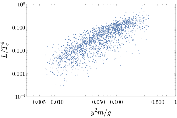
Figure 2: The strength of the phase transition, represented here by the dimensionless $L/T_{\text{c}}^{4}$, is plotted for all the first-order phase transitions in the parameter space studied within our scan, evaluated at $\mathcal{O}({y^{5}})$. It is found to be positively correlated with the ratio $y^{2}m/g$.

$L/T_{\text{c}}^{4}$ is a dimensionless measure of the latent heat, and therefore of the strength of the first-order phase transition. Similarly to the critical temperature, we evaluated this using free energy evaluated to both $\mathcal{O}({y^{2}T^{4}})$ and $\mathcal{O}({y^{5}T^{4}})$. Parameters were run to higher orders, and varied over a range of renormalisation scales, to measure the uncertainty in the predictions.

Fig. 2 plots $L/T_{\text{c}}^{4}$ for consistent first-order phase transitions, with a maximum value of $\sim 0.5$ found in our scan at $\mathcal{O}(y^{5})$. The latent heat is plotted against $y^{2}m/g$, with a strong positive correlation between the two. Since theories with $y^{2}m/g\gtrsim 0.5$ begin to be non-perturbative in our analysis (Fig. 1), a follow up investigation could identify additional, stronger, first-order phase transitions at larger values, for which a different power counting may be necessary, as $y^{2}m/g\sim y$ is no longer small.

4 Comparing results to leading order

The calculations in this work have been carried out to three powers of $y$ beyond leading order, as set out in equations (8) and (11). This section will investigate the size and properties of the sub-leading corrections in the context of the properties of first-order phase transitions.

A number of works have found large discrepancies between calculations of phase transition parameters at low perturbative orders. For example, in the $Z_{2}$-symmetric limit of the real-scalar-extended SM, refs. Carena:2019une ; Ellis:2022lft have found huge discrepancies between computations of the effective potential at order $\mathcal{O}(y^{2}T^{4})$ and $\mathcal{O}(y^{3}T^{4})$. Ref. Gould:2021oba found significantly reduced uncertainties in this model at order $\mathcal{O}(y^{4}T^{4})$. Around the critical temperature, properties of the phase transitions are highly sensitive to additional sub-leading terms, contributing to large corrections to the properties of expected gravitational waves.

4.1 Additional strong phase transitions

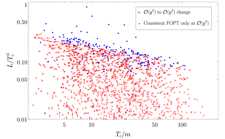
Figure 3: The blue points show theories which are only consistent first-order phase transitions (i.e. valid across renormalisation scales) at $\mathcal{O}({y^{5}})$ and not at $\mathcal{O}({y^{2}})$, using power counting as per eqs. (8) and (11). For consistent first-order phase transitions at both $\mathcal{O}({y^{2}})$ and $\mathcal{O}({y^{5}})$, the changes due to loop corrections for the latent heat and critical temperatures are plotted as red arrows. There are no parameter points that are consistent first-order phase transitions at leading order but not at $\mathcal{O}({y^{5}})$.

Across different renormalisation scales, there may not be only quantitative differences in the values of properties such as latent heat, but also qualitative differences in the predicted nature of the phase transition. This can mean for example that a particularly theory has a first-order phase transition at one renormalisation scale, but becomes a crossover when evaluated at another scale.

Figure 4: The leading order calculation failed to identify the majority of the strongest first-order phase transitions found at $\mathcal{O}({y^{5}})$. At one or more renormalisation scales, many of these were found to be not perturbative at leading order — where contributions from the next order are larger than the leading order value of $T_{\text{c}}$. Other strong phase transitions were categorised as crossovers at leading order.

This has been treated in ref. Papaefstathiou:2021glr through a characterisation from “ultra-conservative” to “liberal”, based on the consistency of results with respect to scale. Here we adopt an approach that would be considered “conservative” in this sense, where a theory associated with a set of parameters is considered to be a consistent first-order phase transition if it is true across the range of renormalisation scales $\mu=A\pi T_{\text{c}}$, where $A$ varies over 7 equidistant values from $1/2$ to $2$. The theories shown in blue in fig. 1 are all consistent first-order phase transitions in this sense, whereas points in other categorisations were evaluated to have the corresponding prediction (e.g. crossover) at one or more of the renormalisation scales considered.

It can be seen from figure 3 that a large number of parameter points are only found to be consistent first-order phase transitions with the higher order $\mathcal{O}({y^{5}})$ calculation, and not when evaluated at leading order, $\mathcal{O}({y^{2}})$. The higher loop order calculation significantly changes the landscape of strong first-order phase transitions. The additional first-order phase transitions at $\mathcal{O}({y^{5}})$ in our scan correspond to a 57% increase in FOPTs with $L/T_{\text{c}}^{4}>0.1$ (from 229 to 359), or a 270% increase in FOPTs with $L/T_{\text{c}}^{4}>0.2$ (from 19 to 71).

Figure 4 plots the same points, now also indicating the nature of the theories which are consistent first-order phase transitions at $\mathcal{O}({y^{5}})$, but not at $\mathcal{O}({y^{2}})$, for at least one renormalisation scale. Over half of these are due to non-perturbative corrections when evaluated at leading order, with running at $\mathcal{O}({y^{4}})$, as defined in section 3.3.

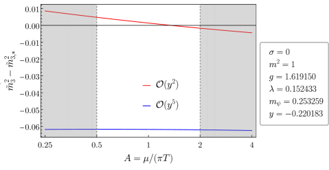
(a)

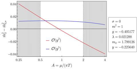
(b)

Figure 5: Two parameters points which at $\mathcal{O}({y^{2}})$ are either crossovers or FOPTs, depending on renormalisation scale choice, are found at $\mathcal{O}({y^{5}})$ to be consistently FOPT(a) and crossover(b) irrespective of renormalisation scale.

Most of the remainder are predicted to be crossovers ($\tilde{m}_{3}^{2}-\tilde{m}_{3,*}^{2}>0$) for at least some part of the renormalisation scale range at leading order. Two example parameter points are shown in figure 5. In both cases, the $\mathcal{O}({y^{2}})$ evaluation indicates either a crossover ($\tilde{m}_{3}^{2}-\tilde{m}_{3,*}^{2}>0$) or a first-order phase transition ($\tilde{m}_{3}^{2}-\tilde{m}_{3,*}^{2}<0$), depending on the renormalisation scale used. Therefore, neither point is considered to be a consistent first-order phase transition at leading order. Using the $\mathcal{O}({y^{5}})$ calculation, the parameter point in figure LABEL:fig:benchmarks_crossover_to_fopt is confirmed to be a first-order phase transition, whereas the example in figure LABEL:fig:benchmarks_crossover_to_crossover is found to be consistently a crossover across the renormalisation scales considered. If their natures were determined using only the $\mathcal{O}({y^{2}})$ calculation at a single renormalisation scale $\mu=\pi T$, the parameter point in figure LABEL:fig:benchmarks_crossover_to_fopt would be determined as a crossover, and the point in figure LABEL:fig:benchmarks_crossover_to_crossover a first-order phase transition, both opposites of the conclusions of the $\mathcal{O}({y^{5}})$ calculation.

4.2 Movement of phase transitions

Figure 3 also shows the change in latent heat and critical temperature for all consistent first-order phase transitions identified at both leading order and $\mathcal{O}({y^{5}})$. The red arrows visualise distinctive flows of the higher order contributions in the latent heat and critical temperature plane for our parameter space scan. The latent heat corrections are generally positive, for phase transitions at lower critical temperature, and negative for those at higher critical temperature. The critical temperature corrections are generally negative. This pattern of flow means that a given set of theories occupying some parameter space, is transported as a whole in the latent heat and critical temperature plane, as a result of including higher order contributions. In other words, the blob moves, at least in the context of our scan.

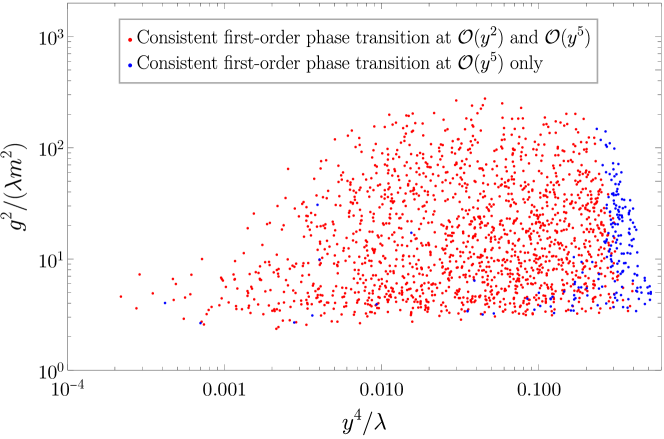
Figure 6: From $\mathcal{O}({y^{2}})$ to $\mathcal{O}({y^{5}})$, consistent first-order phase transitions expand in our scan’s theory parameter space to include points with larger Yukawa couplings relative to $\lambda$.

As well as in the space of the physics predictions of the theory, it is also possible to study the transport of predictions in parameter space when higher order contributions are added. Figure 6 plots theories predicted to be first-order phase transitions at $\mathcal{O}({y^{2}})$ and $\mathcal{O}({y^{5}})$, with power counting as before per eqs. (8) and (11), against combinations of parameters $y^{4}/\lambda$ and $g^{2}/(\lambda m^{2})$. These are the same combinations as fig. 1, where they are found to be correlated with the type of phase transition predicted. The figure shows that, for our scan, within the higher order calculation the set of consistent FOPTs extends in the direction of larger $y^{4}/\lambda$, shown in blue. Therefore, in parameter space, the blob grows, but does not move, in the context of our scan.

At larger still values $y^{4}/\lambda\sim\pi^{2}$, 1-loop contributions from the Yukawa interaction compete with the tree-level scalar self-coupling in the zero-temperature effective potential. In this case a new set of power counting relations, and consequently resummations, are required for the perturbative description Coleman:1973jx ; Weinberg:1992ds ; Kierkla:2022odc .

4.3 Reduced errors

Figure 7: There is generally a reduction in error in predictions of the latent heat at $\mathcal{O}({y^{5}})$ compared to $\mathcal{O}({y^{2}})$, in our scan, for theories that are consistent first-order phase transitions at both orders.

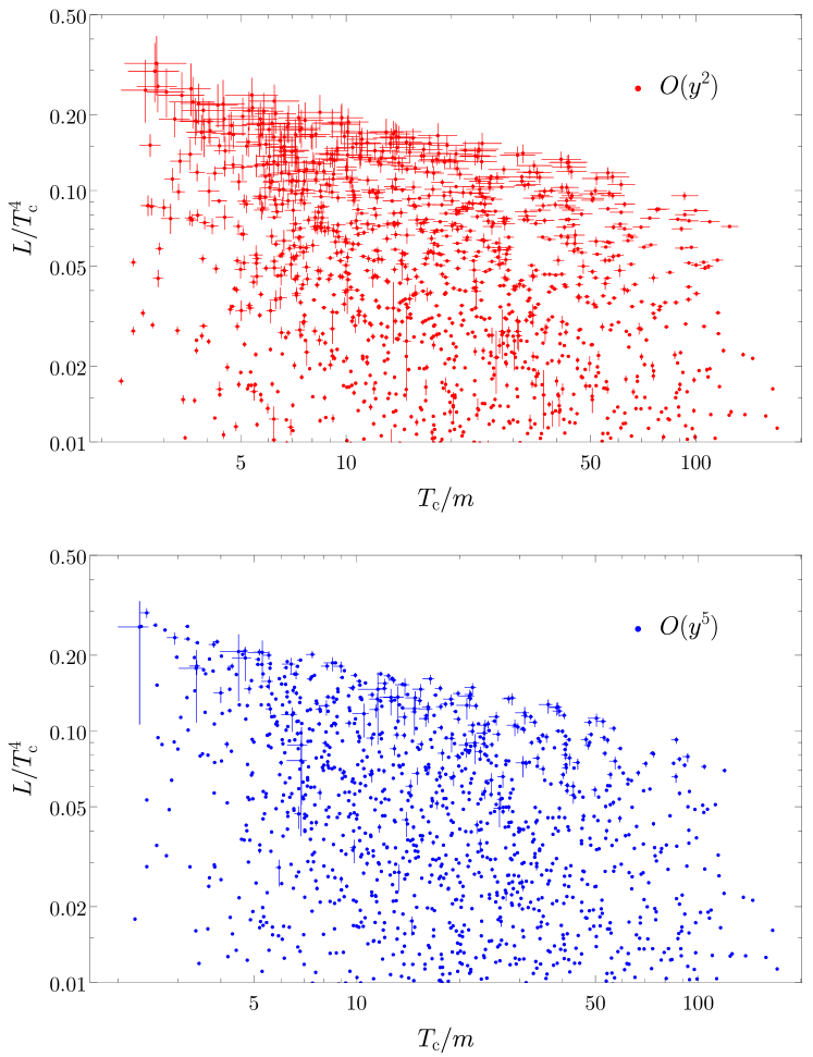
Figure 8: $T_{\text{c}}/m$ and $L/T_{\text{c}}^{4}$ are plotted with their relative errors for theories that are consistent FOPTs when evaluated with $f$ at both $\mathcal{O}({y^{2}T^{4}})$ and $\mathcal{O}({y^{5}T^{4}})$. There is a large reduction in relative error at higher order, especially for strong phase transitions, for our scan. There are also a number of points where the LO result underestimated the error.

Figs. 7 and 8 show relative errors for theories that are consistent first-order phase transitions, when evaluated at both $\mathcal{O}({y^{2}})$ and $\mathcal{O}({y^{5}})$ in the counting of eq. (11). The uncertainties were determined by varying the renormalisation scale between $\mu=\pi T/2$ and $\mu=2\pi T$.

Fig. 7 shows that nearly all of the theory space benefits from reduced uncertainty at higher order. It is instructive to focus on the strongest first-order phase transitions, as only these are expected to yield gravitational wave signatures which are observable by next-generation detectors Gowling:2021gcy ; Boileau:2022ter . This can be seen in fig. 8.

The errors are in general larger for the strongest transitions. For first-order phase transitions in our scan that are both strong (with $L/T^{4}>0.1$) and consistent in both calculations, the higher order calculation reduces the average relative range in critical temperature from 18% to 4%, in latent heat from 19% to 6% and in $\tilde{m}_{3}^{2}-\tilde{m}_{3,*}^{2}$ from 19% to 7%. If we considered even stronger phase transitions, with $L/T^{4}>0.2$, the higher order calculation reduces the average relative range in critical temperature from 28% to 7%, in latent heat from 40% to 16% and in $\tilde{m}_{3}^{2}-\tilde{m}_{3,*}^{2}$ from 13% to 5%.

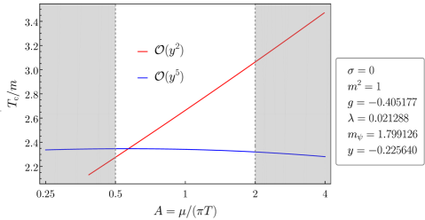
(a)

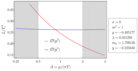
(b)

Figure 9: Uncertainties in $T_{\text{c}}$ and $L/T_{\text{c}}^{4}$ are significantly reduced when evaluating using the free energy density to $\mathcal{O}({y^{5}T^{4}})$  here shown for a benchmark point with a strong transition.

Figure 9 provides an example of a strong first order phase transition. The uncertainties in the critical temperature and the strength of the phase transition were significantly reduced at $\mathcal{O}({y^{5}})$ compared to the leading order $\mathcal{O}({y^{2}})$ evaluation. Note that below the scale choice $A\sim 0.4$, these quantities are not evaluated at $\mathcal{O}({y^{2}})$ as the parameter point is found to receive non-perturbative corrections to the critical temperature. Since this is outside of the range $1/2\leq A\leq 2$, this parameter point is still considered a consistent first-order phase transition at $\mathcal{O}({y^{2}})$.

As well as a reduction in uncertainty, it can be seen from figure 8 that a small number of theories have larger estimated errors when evaluated for the higher order calculation. This reveals an underestimate of the uncertainty associated with the perturbative calculation when evaluated at leading order, and is another improvement offered by the calculation computing free energy density up to $\mathcal{O}({y^{5}T^{4}})$. Interestingly, the lower half of the $\mathcal{O}({y^{2}})$ plot resembles the $\mathcal{O}({y^{5}})$ plot, when the former is scaled up by a factor of $5\sim 10$, i.e. an order of magnitude.

A “conservative” approach was adopted here, where a first-order phase transitions is required to be consistently identified across a range of renormalisation scales. A similar story emerges if a more “liberal” approach is taken, such as evaluating the nature of the theory only at a single renormalisation scale, for example setting $A=1$. Another option is to include a theory as a first-order phase transition if it is evaluated as such for any subset of the renormalisation scale range considered. Using each of these alternative approaches, applied to our scan, the calculation at $\mathcal{O}({y^{5}})$ evaluates additional strong phase transitions not identified at leading order using the same approach, combined with reduced relative error in the critical temperature and latent heat evaluated.

5 Discussion

Let us outline an answer to the central question of our study of cosmological phase transitions: how important are higher perturbative orders for a global parameter scan of a model? Previous studies have shown that higher orders are vital for making reliable predictions for cosmological phase transitions at individual benchmark parameter points in a model Kainulainen:2019kyp ; Croon:2020cgk ; Niemi:2020hto ; Niemi:2021qvp ; Gould:2021oba ; Gould:2023ovu . Yet it was unclear if these conclusions would extend to a global parameter scan, or whether higher perturbative orders would merely reshuffle parameter points.

We have tackled these questions using a Yukawa model as our guide. The simplicity of this model has allowed us to push to $\mathcal{O}({y^{5}T^{4}})$ accuracy for the free-energy density. To do so, we have carried out high-temperature dimensional reduction, constructing a 3d effective field theory of only the lightest bosonic modes, and have included relevant infrared contributions up to three loops.

In short, higher orders reduce errors across the board, but are most important for describing the strongest phase transitions, where errors are largest. At leading order, the renormalisation scale dependence of the strongest phase transitions we have identified yield error estimates over 100%, or change the character of the transition from first order through second order to crossover. Only at higher loops can the order of these strongest transitions, and their thermodynamic properties, be computed reliably.

This is expected to significantly impact predictions of the resulting gravitational wave signals, as these depend sensitively on the thermodynamics of the transition. Yet, additional nonequilibrium physics enters the computation of the gravitational wave spectrum, through the bubble nucleation rate and bubble wall speed. The calculation of higher orders for these quantities is in its infancy: for the nucleation rate the $\mathcal{O}(y^{3})$ term has recently moved into reach Ekstedt:2021kyx ; Gould:2021ccf ; Ekstedt:2023sqc , while for the bubble wall speed even a complete leading order calculation would extend the current state-of-the-art, which relies on a leading-log expansion Laurent:2022jrs .

Future work could extend the model to include couplings to the Standard Model through the Higgs portal. Carrying through to explicitly evaluating the consequences for gravitational waves would then yield results directly applicable to the widely studied singlet fermionic dark matter candidate, extending the conclusions of previous works Fairbairn:2013uta ; Li:2014wia ; Beniwal:2018hyi to higher orders. While the question remains as to how to compute higher orders for the nonequilibrium quantities which enter the gravitational wave spectrum, already some relevant information can be gleaned by upgrading the equilibrium calculation.

A natural question to ask next is: to what extent do we expect our conclusions to apply to other models? Crucially, strong first-order phase transitions are associated with large couplings and large errors also in scalar extensions of the Standard Model Caprini:2015zlo ; Gould:2021oba ; Niemi:2021qvp ; Niemi:2020hto ; Gould:2023ovu , as well as in the Standard Model Effective Field Theory Croon:2020cgk . Therefore, it seems plausible that the broad brushstrokes of our conclusions may apply to many other models, at least when the structure of the power counting relations is similar, that is, when the transitioning field is of the soft scale $m_{\text{eff}}\sim yT$. However, there may be qualitative differences for symmetry-breaking transitions, where the transitioning field instead lives at the supersoft scale $m_{\text{eff}}\sim y^{3/2}T/\pi$ Gould:2021ccf ; Hirvonen:2022jba ; Ekstedt:2022zro ; Lofgren:2023sep , or for very strong phase transitions where additional hierarchies of scale occur Kierkla:2022odc ; Gould:2023ovu .

Appendix A Power counting prescription

At high temperatures, thermal fluctuations (loops) qualitatively change the structure of the effective potential. At such temperatures, the vanilla loop expansion breaks down but one can still make progress by counting powers of couplings. To do so in a theory with multiple couplings, it is useful to fix power counting relations between the couplings.

To start with we assume that all three interaction terms are approximately equally perturbative. This assumption anyway underlies the usual loop expansion at zero temperature, and amounts to parametrically equating the loop expansion parameters for each interaction

$$\lambda\sim y^{2}\sim\frac{g^{2}}{m^{2}}.$$ (39)

The latter two terms are squared because each additional loop requires two cubic interactions, but only one quartic interaction, and follows from standard graph theoretic results Peskin:1995ev . The inverse powers of $m$ in the last term are necessary to cancel the dimensions of $g$, and arise from loop integrals of $\phi$. Note that we have not made explicit the factors of $1/(4\pi)$ arising from loop integrations.

In addition, we will assume that the leading effects of high-temperature fluctuations are of the same size as the tree-level scalar potential. For the scalar tadpole and mass, this amounts to

$$\frac{\sigma}{T^{2}} \sim g\ , \frac{m^{2}}{T^{2}} \sim\lambda\ .$$ (40)

This assumption is natural in the vicinity of a phase transition, as thermal fluctuations must balance against tree-level terms.

Finally, we must make an assumption about the fermion mass, $m_{\psi}$. For the fermion to have any effect on a phase transition, its mass cannot be large compared with the temperature. Otherwise its effects would be exponentially (Boltzmann) suppressed. For simplicity, we will power count the fermion mass the same as the scalar mass,

$$m_{\psi}\sim m\ .$$ (41)

Our analysis will nevertheless include $m_{\psi}\ll m$ as a special case.

In summary, we adopt the following power counting prescription:

$$\frac{\sigma}{T^{3}}\sim\frac{m^{2}}{T^{2}}\sim\frac{g}{T}\sim\lambda\sim y^{2}\sim\frac{m_{\psi}^{2}}{T^{2}}\ .$$ (42)

A generic equilibrium observable $\theta$ has an expansion of the form $\theta/\theta_{\text{LO}}=1+c_{1}y+c_{2}y^{2}+c_{3}y^{3}+\dots$, and in this work we calculate up to and including the $c_{3}y^{3}$ term. For the effective potential and latent heat, which are $\mathcal{O}({y^{2}T^{4}})$ at leading order, this means evaluation to $\mathcal{O}({y^{5}T^{4}})$, or equivalently $\mathcal{O}({\lambda^{5/2}T^{4}})$, with errors of $\mathcal{O}({y^{6}T^{4}})$. For the critical temperature, $\mathcal{O}({my^{-1}})$ at leading order, the evaluation is to $\mathcal{O}({my})$ as there is in general no contribution at $\mathcal{O}({my^{2}})$, with errors of $\mathcal{O}({my^{3}})$.

Appendix B Evaluating and matching correlation functions

We evaluated the connected, one-particle irreducible correlation functions, denoted by $\Gamma^{(k)}$ in the 4d theory and $\Gamma_{3}^{(k)}$ in the 3d effective theory. These observables were then be used to derive matching relations between the theories to find expressions for the effective parameters.

In constructing the EFT Manohar:2018aog ; Burgess:2020tbq , we are aiming to capture the averaged effect of the hard scale modes ($\sim\pi T$) on the soft scale modes ($\sim yT$). As such, in the computation of correlation functions we are free to cut off the soft modes in any way, as long as we do so on both sides of the matching relations. This observation underlies the strict perturbation theory approach of Braaten and Nieto Braaten:1995cm , which we follow. Essentially one expands all loop integrals in powers of the soft scale, and then uses dimensional regularisation to cut off any infrared divergences. In this context, matching correlation functions is equivalent to directly integrating out the hard modes Burgess:2020tbq ; Hirvonen:2022jba .

The one, two, three and four-point correlation functions are given by the sum of diagrams in figs. 10, 11, 12 and 13 respectively. These were generated using FeynArts Kublbeck:1990xc . Only diagrams and terms up to order $\mathcal{O}(y^{5})$ in the power counting prescription eq. (8) were included in the calculations. Tadpole and mass terms are treated as interactions, according to strict perturbation theory, due to the hierarchy of energy scales between their coefficients and $\pi T$ which characterises the free Lagrangian. The results of the loop sum integrals can be found in the literature and are listed in appendix C.

The evaluation of the correlation functions are given in equations (B) to (53). The Euler-Mascheroni constant is denoted by $\gamma_{E}$, and $A$ is the Glaisher-Kinkelin constant. Zero-temperature counterterms, given in appendix D, are used in the evaluation to cancel the temperature independent divergences. In order to simplify the formulae, we have also introduced notation following Kajantie:1995dw :

$$L_{b}(\Lambda)\equiv 2\log\left(\frac{e^{\gamma_{E}}\Lambda}{4\pi T}\right)$$ (43)

$$L_{f}(\Lambda)\equiv 2\log\left(\frac{e^{\gamma_{E}}\Lambda}{\pi T}\right)$$ (44)

$$c\equiv-\log\left(\frac{3e^{\gamma_{E}/2}A^{6}}{4\pi}\right)=-0.348723...$$ (45)

$$\begin{aligned} \mathllap{\Gamma^{(1)}(\mathbf{0})}&\approx\sigma+\delta\sigma+\frac{1}{2}g\sumint_{\,Q}\frac{1}{Q^{2}}-\frac{1}{4}g\lambda\sumint_{\,QR}\frac{1}{Q^{2}R^{4}}-\frac{1}{6}g\lambda\sumint_{\,QR}\frac{1}{Q^{2}R^{2}(Q+R)^{2}}\end{aligned}$$

$$\begin{aligned} &\quad+\frac{1}{2}\delta g\sumint_{\,Q}\frac{1}{Q^{2}}-\frac{1}{2}g(m^{2}+\delta m^{2})\sumint_{\,Q}\frac{1}{Q^{4}}-\frac{1}{2}g\delta Z\sumint_{\,Q}\frac{1}{Q^{2}}\end{aligned}$$

$$\begin{aligned} &\quad+iy\sumint_{\,\{Q\}}\frac{\text{Tr}[\not{Q}]}{Q^{2}}+i\delta y\sumint_{\,\{Q\}}\frac{\text{Tr}[\not{Q}]}{Q^{2}}-y(m_{\psi}+\delta m_{\psi})\sumint_{\,\{Q\}}\frac{\text{Tr}[\not{Q}\not{Q}]}{Q^{4}}\end{aligned}$$

$$\begin{aligned} &\quad-iy\delta Z_{f}\sumint_{\,\{Q\}}\frac{\text{Tr}[\not{Q}\not{Q}\not{Q}]}{Q^{4}}-\delta ym_{\psi}\sumint_{\,\{Q\}}\frac{\text{Tr}[\not{Q}\not{Q}]}{Q^{4}}\end{aligned}$$ (46)

$$\begin{aligned} &\quad+ym_{\psi}^{3}\sumint_{\,\{Q\}}\frac{\text{Tr}[\not{Q}\not{Q}\not{Q}\not{Q}]}{Q^{8}}+2ym_{\psi}\delta Z_{f}\sumint_{\,\{Q\}}\frac{\text{Tr}[\not{Q}\not{Q}\not{Q}\not{Q}]}{Q^{6}}\end{aligned}$$

$$\begin{aligned} &\quad-iy^{3}\sumint_{\,\{QR\}}\frac{\text{Tr}[\not{Q}\not{R}\not{Q}]}{Q^{4}(Q-R)^{2}R^{2}}+2y^{3}m_{\psi}\sumint_{\,\{QR\}}\frac{\text{Tr}[\not{Q}\not{R}\not{Q}\not{Q}]}{Q^{6}(Q-R)^{2}R^{2}}\end{aligned}$$

$$\begin{aligned} &\quad+y^{3}m_{\psi}\sumint_{\,\{QR\}}\frac{\text{Tr}[\not{Q}\not{Q}\not{R}\not{R}]}{Q^{4}(Q-R)^{2}R^{4}}+\frac{1}{2}gy^{2}\sumint_{\,\{QR\}}\frac{\text{Tr}[\not{Q}\not{R}]}{Q^{2}(Q-R)^{4}R^{2}}\end{aligned}$$

$$\begin{aligned} &\approx\sigma+\frac{gT^{2}}{24}+\frac{1}{(4\pi)^{2}}\bigg{[}\frac{1}{6}g\lambda T^{2}\Big{(}\frac{1}{4\epsilon}+\frac{1}{8}L_{b}(\Lambda)+6\log(A)-\frac{1}{2}\gamma_{E}\Big{)}\\ &\quad-\frac{1}{2}gm^{2}L_{b}(\Lambda)\bigg{]}+\frac{m_{\psi}yT^{2}}{6}+\frac{1}{(4\pi)^{2}}\bigg{[}4ym_{\psi}^{3}L_{f}(\Lambda)\\ &\quad+\frac{gT^{2}y^{2}}{24}(L_{f}(\Lambda)-3L_{b}(\Lambda))+\frac{m_{\psi}T^{2}y^{3}}{6}(L_{f}(\Lambda)+2L_{b}(\Lambda))\bigg{]}\end{aligned}$$ (47)

(a)

(b)

(c)

(d)

(e)

(f)

(g)

(h)

(i)

(j)

(k)

(l)

(m)

(n)

(o)

(p)

Figure 10: The Feynman diagrams contributing to the one-point correlation function, $\Gamma^{(1)}(\mathbf{0})$ up to $\mathcal{O}(y^{4}T^{3})$, with power counting set out in eq. (8).

(a)

(b)

(c)

(d)

(e)

(f)

(g)

(h)

(i)

(j)

(k)

(l)

(m)

(n)

(o)

(p)

(q)

(r)

Figure 11: The Feynman diagrams contributing to the two-point correlation function, $\Gamma^{(2)}(\mathbf{p,-p})$ up to $\mathcal{O}(y^{4}T^{2})$.

$$\begin{aligned} \mathllap{\Gamma^{(2)}(\mathbf{p,-p})}&\approx p^{2}+m^{2}+\delta m^{2}+p^{2}\delta Z+\frac{\lambda}{2}\sumint_{\,Q}\frac{1}{Q^{2}}-\frac{g^{2}}{2}\sumint_{\,Q}\frac{1}{Q^{4}}\left(1-\frac{p^{2}}{Q^{2}}+\frac{4(\mathbf{p\cdot q})^{2}}{Q^{4}}\right)\end{aligned}$$

$$\begin{aligned} &\quad-\frac{\lambda^{2}}{4}\sumint_{\,QR}\frac{1}{Q^{4}R^{2}}-\frac{\lambda^{2}}{6}\sumint_{\,QR}\frac{1}{Q^{2}R^{2}(Q+R)^{2}}+\frac{\delta\lambda}{2}\sumint_{\,Q}\frac{1}{Q^{2}}\end{aligned}$$

$$\begin{aligned} &\quad-g\delta g\sumint_{\,Q}\frac{1}{Q^{4}}-\frac{\lambda}{2}(m^{2}+\delta m^{2})\sumint_{\,Q}\frac{1}{Q^{4}}-\frac{\lambda}{2}\delta Z\sumint_{\,Q}\frac{Q^{2}}{Q^{4}}\end{aligned}$$

$$\begin{aligned} &\quad+g^{2}(m^{2}+\delta m^{2})\sumint\frac{1}{Q^{6}}-4y^{2}\sumint_{\,\{Q\}}\frac{1}{Q^{2}}\left(1-\frac{p^{2}}{Q^{2}}+\frac{2(\mathbf{p\cdot q})^{2}}{Q^{4}}\right)\end{aligned}$$ (48)

$$\begin{aligned} &\quad-2iy^{2}(m_{\psi}+\delta m_{\psi})\sumint_{\,\{Q\}}\frac{\text{Tr}[\not{Q}\not{Q}\not{Q}]}{Q^{6}}+2y^{2}\delta Z_{f}\sumint_{\,\{Q\}}\frac{\text{Tr}[\not{Q}\not{Q}\not{Q}\not{Q}]}{Q^{6}}\end{aligned}$$

$$\begin{aligned} &\quad-2y\delta y\sumint_{\,\{Q\}}\frac{\text{Tr}[\not{Q}\not{Q}]}{Q^{4}}+y^{2}m_{\psi}^{2}\sumint_{\,\{Q\}}\frac{\text{Tr}[\not{Q}\not{Q}\not{Q}\not{Q}]}{Q^{8}}\end{aligned}$$

$$\begin{aligned} &\quad+2y^{2}m_{\psi}^{2}\sumint_{\,\{Q\}}\frac{\text{Tr}[\not{Q}\not{Q}\not{Q}\not{Q}]}{Q^{8}}+y^{4}\sumint_{\,\{QR\}}\frac{\text{Tr}[\not{Q}\not{Q}\not{R}\not{R}]}{Q^{4}(Q-R)^{2}R^{4}}\end{aligned}$$

$$\begin{aligned} &\quad+2igy^{3}\sumint_{\,\{QR\}}\frac{\text{Tr}[\not{Q}\not{Q}\not{R}]}{Q^{4}(Q-R)^{4}R^{2}}+2y^{4}\sumint_{\,\{QR\}}\frac{\text{Tr}[\not{Q}\not{Q}\not{Q}\not{R}]}{Q^{6}(Q-R)^{2}R^{2}}\end{aligned}$$

$$\begin{aligned} &\quad+\frac{1}{2}\lambda y^{2}\sumint_{\,\{QR\}}\frac{\text{Tr}[\not{Q}\not{R}]}{Q^{2}(Q-R)^{4}R^{2}}\end{aligned}$$

$$\begin{aligned} &\approx p^{2}+m^{2}+\frac{\lambda T^{2}}{24}-\frac{g^{2}L_{b}(\Lambda)}{2(4\pi)^{2}}\\ &\quad+\frac{1}{(4\pi)^{2}}\bigg{[}\frac{\lambda^{2}T^{2}}{12}\Big{(}\frac{1}{2\epsilon}+\frac{L_{b}(\Lambda)}{4}-\gamma_{E}+12\log(A)\Big{)}-\frac{\lambda m^{2}}{2}L_{b}(\Lambda)\bigg{]}\\ &\quad+\frac{y^{2}}{6(4\pi)^{2}}\bigg{[}8p^{2}+16T^{2}\pi^{2}+L_{f}(\Lambda)\Big{(}72m_{\psi}^{2}+12p^{2}+y^{2}T^{2}+\frac{\lambda T^{2}}{4}\Big{)}\\ &\quad+L_{b}(\Lambda)\Big{(}2y^{2}T^{2}-\frac{3\lambda T^{2}}{4}\Big{)}\bigg{]}\end{aligned}$$ (49)

(a)

(b)

(c)

(d)

Figure 12: The Feynman diagrams contributing to the three-point correlation function, $\Gamma^{(3)}(\mathbf{p,q,-p,-q})$ up to $\mathcal{O}(y^{4}T)$.

$$\begin{split}\Gamma^{(3)}(\mathbf{p,q,-p,-q})\approx{}&g+\delta g-\frac{3}{2}g\lambda\sumint_{\,Q}\frac{1}{Q^{4}}-2iy^{3}\sumint_{\,Q}\frac{\text{Tr}[\not{Q}\not{Q}\not{Q}]}{Q^{6}}\\ &+6y^{3}m_{\psi}\sumint_{\,Q}\frac{\text{Tr}[\not{Q}\not{Q}\not{Q}\not{Q}]}{Q^{8}}\end{split}$$ (50)

$$\begin{split}\approx{}&g-\frac{3}{2(4\pi)^{2}}g\lambda L_{b}(\Lambda)+\frac{24y^{3}m_{\psi}}{(4\pi)^{2}}L_{f}(\Lambda)\end{split}$$ (51)

(a)

(b)

(c)

Figure 13: The Feynman diagrams contributing to the four-point correlation function, $\Gamma^{(4)}(\mathbf{p,q,r,-p,-q,-r})$ up to $\mathcal{O}(y^{4})$.

$$\begin{split}\Gamma^{(4)}(\mathbf{p,q,r,-p,-q,-r})\approx{}&\lambda+\delta\lambda-\frac{3}{2}\lambda^{2}\sumint_{\,Q}\frac{1}{Q^{4}}+6y^{4}\sumint_{\,Q}\frac{\text{Tr}[\not{Q}\not{Q}\not{Q}\not{Q}]}{Q^{8}}\end{split}$$ (52)

$$\begin{split}\approx{}&\lambda-\frac{3}{2(4\pi)^{2}}\lambda^{2}L_{b}(\Lambda)+\frac{24y^{4}}{(4\pi)^{2}}L_{f}(\Lambda)\end{split}$$ (53)

In evaluating these equations we expanded assuming $p\sim yT$. Performing the same calculation in the effective theory, and using the vanishing of scaleless integrals in dimensional regularisation, we find trivially that,

$$\begin{split}\Gamma_{3}^{(1)}(\mathbf{0})\approx{}&\sigma_{3}+\delta\sigma_{3}\end{split}$$ (54)

$$\begin{split}\Gamma_{3}^{(2)}(\mathbf{p,-p})\approx{}&p^{2}+m_{3}^{2}+\delta m_{3}^{2}\end{split}$$ (55)

$$\begin{split}\Gamma_{3}^{(3)}(\mathbf{p,q,-p,-q})\approx{}&g_{3}+\delta g_{3}\end{split}$$ (56)

$$\begin{split}\Gamma_{3}^{(4)}(\mathbf{p,q,r,-p,-q,-r})\approx{}&\lambda_{3}+\delta\lambda_{3}\ \text{.}\end{split}$$ (57)

Following ref. Kajantie:1995dw , we match the leading momentum dependence of the correlation functions through a field normalisation, as well as equate the 1 to 4 point correlation functions at zero momentum between the full and effective theories. Using these relationships we arrive at the expressions (12) to (16) for the 3d EFT parameters. The following counterterms are required in the 3d theory to cancel against the temperature dependent poles from the full theory,

$$\begin{split}\delta\sigma_{3}={}&\frac{g_{3}\lambda_{3}}{24(4\pi)^{2}\epsilon}\ ,\end{split}$$ (58)

$$\begin{split}\delta m_{3}^{2}={}&\frac{\lambda_{3}^{2}}{24(4\pi)^{2}\epsilon}\ .\end{split}$$ (59)

Appendix C Loop integrals

In $d=3-2\epsilon$ dimensions, the loop integral measure is defined as

$$\int_{p}\equiv\left(\frac{e^{\gamma}\Lambda^{2}}{4\pi}\right)^{\epsilon}\int\frac{d^{3-2\epsilon}p}{\left(2\pi\right)^{3-2\epsilon}}\ ,$$ (60)

where $\Lambda$ is the $\overline{\text{MS}}$ renormalisation scale. In $d=4-2\epsilon$, the loop integration measure is defined analogously. Sum integrals over loop momenta are defined as,

$$\sumint_{\,P\text{ or }\{P\}}\equiv T\sum_{n=-\infty}^{\infty}\int_{p}\ ,$$ (61)

where thermal four momenta are denoted by uppercase letters, $P=(p_{0},p)$, with spatial momenta $p$ and Matsubara frequencies $p_{0}=2\pi Tn$ for bosonic sum integrals (denoted by $P$) and $p_{0}=(2n+1)\pi T$ for fermionic sum integrals (denoted by $\{P\}$).

Massless 1-loop bosonic integrals can be evaluated using the following master sum-integral,

$$\sumint_{\,P}\frac{(p_{0}^{2})^{\beta}(p^{2})^{\gamma}}{(P^{2})^{\alpha}}= \left(\frac{e^{\gamma}\Lambda^{2}}{4\pi}\right)^{\epsilon}\frac{2T(2\pi T)^{d-2\alpha+2\beta+2\gamma}}{(4\pi)^{d/2}}$$

$$\qquad\cdot\frac{\Gamma(\frac{d}{2}+\gamma)\Gamma(-\frac{d}{2}+\alpha-\gamma)}{\Gamma(\frac{d}{2})\Gamma(\alpha)}\zeta(-d+2\alpha-2\beta-2\gamma),$$ (62)

where $\zeta$ is the Riemann zeta function. Massless 1-loop fermion sum integrals can be expressed in terms of bosonic sum integrals using the relationship:

$$\sumint_{\,\{Q\}}=2\times\sumint_{\,Q,T/2}-\sumint_{\,Q}\ ,$$ (63)

where the first sum integral on the right side of the equation should have all temperatures substituted $T\rightarrow T/2$.

Massless 2-loop integrals can be evaluated using integration by parts techniques, reducing them to products of 1-loop sum integrals Ghisoiu:2012yk . In changes of variables, the sum or difference of two fermionic variables is a bosonic variable. The following results were used:

$$\begin{split}\sumint_{\,PQ}\frac{1}{P^{2}Q^{2}(P+Q)^{2}}={}&0\end{split}$$ (64)

$$\begin{split}\sumint_{\,PQ}\frac{1}{P^{4}Q^{2}(P+Q)^{2}}={}&-\frac{1}{(d-2)(d-5)}\sumint_{\,PQ}\frac{1}{P^{4}Q^{4}}\end{split}$$ (65)

$$\begin{split}\sumint_{\,PQ}\frac{1}{P^{6}Q^{2}(P+Q)^{2}}={}&-\frac{4}{(d-2)(d-7)}\sumint_{\,PQ}\frac{1}{P^{4}Q^{6}}\end{split}$$ (66)

$$\begin{split}\sumint_{\,PQ}\frac{1}{P^{4}Q^{4}(P+Q)^{2}}={}&0\end{split}$$ (67)

$$\begin{split}\sumint_{\,\{PQ\}}\frac{1}{P^{2}Q^{2}(P-Q)^{2}}={}&0.\end{split}$$ (68)

Appendix D Zero temperature renormalisation

We have used dimensional regularisation, and adopt the following convention for the counterterm Lagrangian,

$$\mathscr{L}_{\text{ct}} =\frac{1}{2}\delta Z\partial_{\mu}\phi\partial^{\mu}\phi-\delta\sigma\phi-\frac{1}{2}\delta m^{2}\phi^{2}-\frac{1}{3!}\delta g\phi^{3}-\frac{1}{4!}\delta\lambda\phi^{4}$$ (69)

$$\quad+\bar{\psi}(i\delta Z_{f}\not{\partial}-\delta m_{\psi})\psi-\delta y\phi\bar{\psi}\psi\ ,$$ (70)

where $\phi$ and $\psi$ are renormalised fields. The total Lagrangian (1) is then modified as $\mathscr{L}\to\mathscr{L}+\mathscr{L}_{\text{ct}}$. The 1-loop counterterms in $d=4-2\epsilon$ dimensions read

$$\delta\sigma =\frac{gm^{2}-8ym_{\psi}^{3}}{2(4\pi)^{2}\epsilon}, \delta m^{2} =\frac{g^{2}+\lambda m^{2}-24y^{2}m_{\psi}^{2}}{2(4\pi)^{2}\epsilon},$$ (71)

$$\delta g =\frac{3g\lambda-48y^{3}m_{\psi}}{2(4\pi)^{2}\epsilon}, \delta\lambda =\frac{3\lambda^{2}-48y^{4}}{2(4\pi)^{2}\epsilon},$$ (72)

$$\delta m_{\psi} =\frac{y^{2}m_{\psi}}{(4\pi)^{2}\epsilon}, \delta y =\frac{y^{3}}{(4\pi)^{2}\epsilon},$$ (73)

$$\delta Z =-\frac{2y^{2}}{(4\pi)^{2}\epsilon}, \delta Z_{f} =-\frac{y^{2}}{2(4\pi)^{2}\epsilon}.$$ (74)

The corresponding beta functions and anomalous dimensions are

$$\beta_{\sigma} =\frac{gm^{2}-8ym_{\psi}^{3}+2\sigma y^{2}}{(4\pi)^{2}}, \beta_{m^{2}} =\frac{g^{2}+\lambda m^{2}+4y^{2}m^{2}-24y^{2}m_{\psi}^{2}}{(4\pi)^{2}},$$ (75)

$$\beta_{g} =\frac{3g\lambda-48y^{3}m_{\psi}+6gy^{2}}{(4\pi)^{2}}, \beta_{\lambda} =\frac{3\lambda^{2}-48y^{4}+8\lambda y^{2}}{(4\pi)^{2}},$$ (76)

$$\beta_{m_{\psi}} =\frac{3y^{2}m_{\psi}}{(4\pi)^{2}}, \beta_{y} =\frac{5y^{3}}{(4\pi)^{2}},$$ (77)

$$\gamma_{\phi} =-\frac{2y^{2}}{(4\pi)^{2}}, \gamma_{\psi} =-\frac{y^{2}}{2(4\pi)^{2}}.$$ (78)

The beta functions for the dimensionless couplings are corroborated by refs. Cheng:1973nv ; Baek:2012uj .

Barred couplings explicitly demonstrating renormalisation scale invariance for the 3d EFT parameters in eqs. (12) to (16) are defined as:

$$\bar{\chi}={} \chi-\frac{1}{2}\beta_{\chi}^{\text{b}}L_{b}(\Lambda)-\frac{1}{2}\beta_{\chi}^{\text{f}}L_{f}(\Lambda),$$ (79)

where for each parameter, the full beta function is equal to the sum of the bosonic and fermionic parts $\beta=\beta^{\text{b}}+\beta^{\text{f}}$, with:

$$\beta_{\sigma}^{\text{b}} =\frac{gm^{2}}{(4\pi)^{2}}, \beta_{\sigma}^{\text{f}} =-\frac{8ym_{\psi}^{3}}{(4\pi)^{2}}+\frac{2y^{2}\sigma}{(4\pi)^{2}},$$ (80)

$$\beta_{m^{2}}^{\text{b}} =\frac{g^{2}}{(4\pi)^{2}}+\frac{\lambda m^{2}}{(4\pi)^{2}}, \beta_{m^{2}}^{\text{f}} =-\frac{24y^{2}m_{\psi}^{2}}{(4\pi)^{2}}+\frac{4y^{2}m^{2}}{(4\pi)^{2}},$$ (81)

$$\beta_{g}^{\text{b}} =\frac{3g\lambda}{(4\pi)^{2}}, \beta_{g}^{\text{f}} =-\frac{48y^{3}m_{\psi}}{(4\pi)^{2}}+\frac{6y^{2}g}{(4\pi)^{2}},$$ (82)

$$\beta_{\lambda}^{\text{b}} =\frac{3\lambda^{2}}{(4\pi)^{2}}, \beta_{\lambda}^{\text{f}} =-\frac{48y^{4}}{(4\pi)^{2}}+\frac{8y^{2}\lambda}{(4\pi)^{2}},$$ (83)

$$\beta_{y}^{\text{b}} =-\frac{2y^{3}}{(4\pi)^{2}}, \beta_{y}^{\text{f}} =\frac{7y^{3}}{(4\pi)^{2}},$$ (84)

$$\beta_{m_{\psi}}^{\text{b}} =-\frac{2y^{2}m_{\psi}}{(4\pi)^{2}}, \beta_{m_{\psi}}^{\text{f}} =\frac{5y^{2}m_{\psi}}{(4\pi)^{2}}.$$ (85)

For $m_{\psi}$ and $y$ there is some arbitrariness in this split, which has been chosen in order to minimise the presence of $\log(2)$ terms in the dimensional reduction relations, equations (12) to (16).

References

- (1) LISA collaboration, Laser Interferometer Space Antenna, arXiv:1702.00786 (2017) [1702.00786].
- (2) W.-H. Ruan, Z.-K. Guo, R.-G. Cai and Y.-Z. Zhang, Taiji program: Gravitational-wave sources, Int. J. Mod. Phys. A 35 (2020) 2050075 [1807.09495].
- (3) TianQin collaboration, TianQin: a space-borne gravitational wave detector, Class. Quant. Grav. 33 (2016) 035010 [1512.02076].
- (4) S. Kawamura et al., The Japanese space gravitational wave antenna: DECIGO, Class. Quant. Grav. 28 (2011) 094011.
- (5) NANOGrav collaboration, The NANOGrav 15 yr Data Set: Search for Signals from New Physics, Astrophys. J. Lett. 951 (2023) L11 [2306.16219].
- (6) G. Hobbs et al., The international pulsar timing array project: using pulsars as a gravitational wave detector, Class. Quant. Grav. 27 (2010) 084013 [0911.5206].
- (7) M. D’Onofrio and K. Rummukainen, Standard model cross-over on the lattice, Phys. Rev. D 93 (2016) 025003 [1508.07161].
- (8) Y. Aoki, G. Endrodi, Z. Fodor, S.D. Katz and K.K. Szabo, The Order of the quantum chromodynamics transition predicted by the standard model of particle physics, Nature 443 (2006) 675 [hep-lat/0611014].
- (9) Y.G. Kim, K.Y. Lee and S. Shin, Singlet fermionic dark matter, JHEP 05 (2008) 100 [0803.2932].
- (10) S. Baek, P. Ko and W.-I. Park, Search for the Higgs portal to a singlet fermionic dark matter at the LHC, JHEP 02 (2012) 047 [1112.1847].
- (11) S. Baek, P. Ko, W.-I. Park and E. Senaha, Vacuum structure and stability of a singlet fermion dark matter model with a singlet scalar messenger, JHEP 11 (2012) 116 [1209.4163].
- (12) S. Esch, M. Klasen and C.E. Yaguna, Detection prospects of singlet fermionic dark matter, Phys. Rev. D 88 (2013) 075017 [1308.0951].
- (13) O. Buchmueller, M.J. Dolan and C. McCabe, Beyond Effective Field Theory for Dark Matter Searches at the LHC, JHEP 01 (2014) 025 [1308.6799].
- (14) M. Klasen and C.E. Yaguna, Warm and cold fermionic dark matter via freeze-in, JCAP 11 (2013) 039 [1309.2777].
- (15) S. Esch, M. Klasen and C.E. Yaguna, A minimal model for two-component dark matter, JHEP 09 (2014) 108 [1406.0617].
- (16) A. Freitas, S. Westhoff and J. Zupan, Integrating in the Higgs Portal to Fermion Dark Matter, JHEP 09 (2015) 015 [1506.04149].
- (17) S. Baek, P. Ko, M. Park, W.-I. Park and C. Yu, Beyond the Dark matter effective field theory and a simplified model approach at colliders, Phys. Lett. B 756 (2016) 289 [1506.06556].
- (18) G. Dupuis, Collider Constraints and Prospects of a Scalar Singlet Extension to Higgs Portal Dark Matter, JHEP 07 (2016) 008 [1604.04552].
- (19) A. Albert et al., Towards the next generation of simplified Dark Matter models, Phys. Dark Univ. 16 (2017) 49 [1607.06680].
- (20) N.F. Bell, G. Busoni and I.W. Sanderson, Self-consistent Dark Matter Simplified Models with an s-channel scalar mediator, JCAP 03 (2017) 015 [1612.03475].
- (21) M. Fairbairn and R. Hogan, Singlet Fermionic Dark Matter and the Electroweak Phase Transition, JHEP 09 (2013) 022 [1305.3452].
- (22) T. Li and Y.-F. Zhou, Strongly first order phase transition in the singlet fermionic dark matter model after LUX, JHEP 07 (2014) 006 [1402.3087].
- (23) A. Beniwal, M. Lewicki, M. White and A.G. Williams, Gravitational waves and electroweak baryogenesis in a global study of the extended scalar singlet model, JHEP 02 (2019) 183 [1810.02380].
- (24) N. Bernal, M. Heikinheimo, T. Tenkanen, K. Tuominen and V. Vaskonen, The Dawn of FIMP Dark Matter: A Review of Models and Constraints, Int. J. Mod. Phys. A 32 (2017) 1730023 [1706.07442].
- (25) C.E. Yaguna and O. Zapata, A minimal model of fermion FIMP dark matter, 2308.05249.
- (26) K. Farakos, K. Kajantie, K. Rummukainen and M.E. Shaposhnikov, 3-D physics and the electroweak phase transition: Perturbation theory, Nucl. Phys. B 425 (1994) 67 [hep-ph/9404201].
- (27) K. Farakos, K. Kajantie, K. Rummukainen and M.E. Shaposhnikov, 3-d physics and the electroweak phase transition: A Framework for lattice Monte Carlo analysis, Nucl. Phys. B 442 (1995) 317 [hep-lat/9412091].
- (28) E. Braaten and A. Nieto, Effective field theory approach to high temperature thermodynamics, Phys. Rev. D 51 (1995) 6990 [hep-ph/9501375].
- (29) K. Kajantie, M. Laine, K. Rummukainen and M.E. Shaposhnikov, Generic rules for high temperature dimensional reduction and their application to the standard model, Nucl. Phys. B 458 (1996) 90 [hep-ph/9508379].
- (30) E. Braaten and A. Nieto, Free energy of QCD at high temperature, Phys. Rev. D 53 (1996) 3421 [hep-ph/9510408].
- (31) D. Croon, O. Gould, P. Schicho, T.V.I. Tenkanen and G. White, Theoretical uncertainties for cosmological first-order phase transitions, JHEP 04 (2021) 055 [2009.10080].
- (32) A. Papaefstathiou and G. White, The electro-weak phase transition at colliders: confronting theoretical uncertainties and complementary channels, JHEP 05 (2021) 099 [2010.00597].
- (33) O. Gould and T.V.I. Tenkanen, On the perturbative expansion at high temperature and implications for cosmological phase transitions, JHEP 06 (2021) 069 [2104.04399].
- (34) P. Athron, C. Balazs, A. Fowlie, L. Morris, G. White and Y. Zhang, How arbitrary are perturbative calculations of the electroweak phase transition?, 2208.01319.
- (35) D. Curtin, J. Roy and G. White, Gravitational waves and tadpole resummation: Efficient and easy convergence of finite temperature QFT, 2211.08218.
- (36) M. Kierkla, A. Karam and B. Swiezewska, Conformal model for gravitational waves and dark matter: a status update, JHEP 03 (2023) 007 [2210.07075].
- (37) M. Carena, Z. Liu and Y. Wang, Electroweak phase transition with spontaneous Z2-breaking, JHEP 08 (2020) 107 [1911.10206].
- (38) J. Ellis, M. Lewicki, M. Merchand, J.M. No and M. Zych, The Scalar Singlet Extension of the Standard Model: Gravitational Waves versus Baryogenesis, 2210.16305.
- (39) T. Gorda, A. Helset, L. Niemi, T.V.I. Tenkanen and D.J. Weir, Three-dimensional effective theories for the two Higgs doublet model at high temperature, JHEP 02 (2019) 081 [1802.05056].
- (40) S. Biondini, P. Schicho and T.V.I. Tenkanen, Strong electroweak phase transition in -channel simplified dark matter models, 2207.12207.
- (41) K. Kajantie, M. Laine, K. Rummukainen and Y. Schroder, The Pressure of hot QCD up to g6 ln(1/g), Phys. Rev. D 67 (2003) 105008 [hep-ph/0211321].
- (42) A. Gynther and M. Vepsalainen, Pressure of the standard model at high temperatures, JHEP 01 (2006) 060 [hep-ph/0510375].
- (43) A. Ekstedt, P. Schicho and T.V.I. Tenkanen, DRalgo: a package for effective field theory approach for thermal phase transitions, 2205.08815.
- (44) D. Cutting, M. Hindmarsh and D.J. Weir, Vorticity, kinetic energy, and suppressed gravitational wave production in strong first order phase transitions, Phys. Rev. Lett. 125 (2020) 021302 [1906.00480].
- (45) F. Giese, T. Konstandin, K. Schmitz and J. van de Vis, Model-independent energy budget for LISA, JCAP 01 (2021) 072 [2010.09744].
- (46) R. Jinno, T. Konstandin and H. Rubira, A hybrid simulation of gravitational wave production in first-order phase transitions, JCAP 04 (2021) 014 [2010.00971].
- (47) M.A. Ajmi and M. Hindmarsh, Thermal suppression of bubble nucleation at first-order phase transitions in the early Universe, Phys. Rev. D 106 (2022) 023505 [2205.04097].
- (48) L. Sagunski, P. Schicho and D. Schmitt, Supercool exit: Gravitational waves from QCD-triggered conformal symmetry breaking, Phys. Rev. D 107 (2023) 123512 [2303.02450].
- (49) P. Athron, L. Morris and Z. Xu, How robust are gravitational wave predictions from cosmological phase transitions?, 2309.05474.
- (50) K. Kainulainen, V. Keus, L. Niemi, K. Rummukainen, T.V.I. Tenkanen and V. Vaskonen, On the validity of perturbative studies of the electroweak phase transition in the Two Higgs Doublet model, JHEP 06 (2019) 075 [1904.01329].
- (51) L. Niemi, M.J. Ramsey-Musolf, T.V.I. Tenkanen and D.J. Weir, Thermodynamics of a Two-Step Electroweak Phase Transition, Phys. Rev. Lett. 126 (2021) 171802 [2005.11332].
- (52) L. Niemi, P. Schicho and T.V.I. Tenkanen, Singlet-assisted electroweak phase transition at two loops, Phys. Rev. D 103 (2021) 115035 [2103.07467].
- (53) T.V.I. Tenkanen and J. van de Vis, Speed of sound in cosmological phase transitions and effect on gravitational waves, JHEP 08 (2022) 302 [2206.01130].
- (54) O. Gould and T.V.I. Tenkanen, Perturbative effective field theory expansions for cosmological phase transitions, 2309.01672.
- (55) J.I. Kapusta and C. Gale, Finite-temperature field theory: Principles and applications, Cambridge Monographs on Mathematical Physics, Cambridge University Press (2011), 10.1017/CBO9780511535130.
- (56) T. Matsubara, A New approach to quantum statistical mechanics, Prog. Theor. Phys. 14 (1955) 351.
- (57) M. Laine and A. Vuorinen, Basics of Thermal Field Theory, vol. 925, Springer (2016), 10.1007/978-3-319-31933-9, [1701.01554].
- (58) J.O. Andersen and M. Strickland, Resummation in hot field theories, Annals Phys. 317 (2005) 281 [hep-ph/0404164].
- (59) J. Löfgren, Stop comparing resummation methods, 2301.05197.
- (60) O. Gould and J. Hirvonen, Effective field theory approach to thermal bubble nucleation, Phys. Rev. D 104 (2021) 096015 [2108.04377].
- (61) O. Gould, Real scalar phase transitions: a nonperturbative analysis, JHEP 04 (2021) 057 [2101.05528].
- (62) X.-p. Sun, Monte Carlo studies of three-dimensional O(1) and O(4) phi**4 theory related to BEC phase transition temperatures, Phys. Rev. E67 (2003) 066702 [hep-lat/0209144].
- (63) M. Laine, M. Meyer and G. Nardini, Thermal phase transition with full 2-loop effective potential, Nucl. Phys. B 920 (2017) 565 [1702.07479].
- (64) L. Allwicher, P. Arnan, D. Barducci and M. Nardecchia, Perturbative unitarity constraints on generic Yukawa interactions, JHEP 10 (2021) 129 [2108.00013].
- (65) S.S. AbdusSalam et al., Simple and statistically sound recommendations for analysing physical theories, Rept. Prog. Phys. 85 (2022) 052201 [2012.09874].
- (66) A. Papaefstathiou and G. White, The Electro-Weak Phase Transition at Colliders: Discovery Post-Mortem, JHEP 02 (2022) 185 [2108.11394].
- (67) S.R. Coleman and E.J. Weinberg, Radiative Corrections as the Origin of Spontaneous Symmetry Breaking, Phys. Rev. D 7 (1973) 1888.
- (68) E.J. Weinberg, Vacuum decay in theories with symmetry breaking by radiative corrections, Phys. Rev. D 47 (1993) 4614 [hep-ph/9211314].
- (69) C. Gowling and M. Hindmarsh, Observational prospects for phase transitions at LISA: Fisher matrix analysis, JCAP 10 (2021) 039 [2106.05984].
- (70) G. Boileau, N. Christensen, C. Gowling, M. Hindmarsh and R. Meyer, Prospects for LISA to detect a gravitational-wave background from first order phase transitions, JCAP 02 (2023) 056 [2209.13277].
- (71) A. Ekstedt, Higher-order corrections to the bubble-nucleation rate at finite temperature, Eur. Phys. J. C 82 (2022) 173 [2104.11804].
- (72) A. Ekstedt, O. Gould and J. Hirvonen, BubbleDet: A Python package to compute functional determinants for bubble nucleation, 2308.15652.
- (73) B. Laurent and J.M. Cline, First principles determination of bubble wall velocity, Phys. Rev. D 106 (2022) 023501 [2204.13120].
- (74) C. Caprini et al., Science with the space-based interferometer eLISA. II: Gravitational waves from cosmological phase transitions, JCAP 04 (2016) 001 [1512.06239].
- (75) J. Hirvonen, Intuitive method for constructing effective field theories, 2205.02687.
- (76) A. Ekstedt, O. Gould and J. Löfgren, Radiative first-order phase transitions to next-to-next-to-leading order, Phys. Rev. D 106 (2022) 036012 [2205.07241].
- (77) M.E. Peskin and D.V. Schroeder, An Introduction to quantum field theory, Addison-Wesley, Reading, USA (1995).
- (78) A.V. Manohar, Introduction to Effective Field Theories, 1804.05863.
- (79) C.P. Burgess, Introduction to Effective Field Theory, Cambridge University Press (12, 2020), 10.1017/9781139048040.
- (80) J. Kublbeck, M. Bohm and A. Denner, Feyn Arts: Computer Algebraic Generation of Feynman Graphs and Amplitudes, Comput. Phys. Commun. 60 (1990) 165.
- (81) I. Ghisoiu and Y. Schroder, A New Method for Taming Tensor Sum-Integrals, JHEP 11 (2012) 010 [1208.0284].
- (82) T.P. Cheng, E. Eichten and L.-F. Li, Higgs Phenomena in Asymptotically Free Gauge Theories, Phys. Rev. D 9 (1974) 2259.