Discovering Symmetry Breaking in Physical Systems with
Relaxed Group Convolution

Abstract

Modeling symmetry breaking is essential for understanding the fundamental changes in the behaviors and properties of physical systems, from microscopic particle interactions to macroscopic phenomena like fluid dynamics and cosmic structures. Thus, identifying sources of asymmetry is an important tool for understanding physical systems. In this paper, we focus on learning asymmetries of data using relaxed group convolutions. We provide both theoretical and empirical evidence that this flexible convolution technique allows the model to maintain the highest level of equivariance that is consistent with data and discover the subtle symmetry-breaking factors in various physical systems. We employ various relaxed group convolution architectures to uncover various symmetry-breaking factors that are interpretable and physically meaningful in different physical systems, including the phase transition of crystal structure, the isotropy and homogeneity breaking in turbulent flow, and the time-reversal symmetry breaking in pendulum systems.

1 Introduction

Symmetry play pivotal roles in the advancement of deep learning (Zhang, 1988; Kondor & Trivedi, 2018; Bronstein et al., 2021; Cohen & Welling, 2016a; Weiler & Cesa, 2019; Zaheer et al., 2017; Cohen & Welling, 2016b). Specifically, equivariant convolution (Cohen & Welling, 2016b; Esteves et al., 2018) and graph neural networks (Satorras et al., 2021a; Thomas et al., 2018; Cohen et al., 2019), which integrate symmetries into the design of the architectures, have demonstrated notable success in modeling complex data. By constructing a model inherently equivariant to the symmetry group governing transformations of a physical system, we ensure automatic generalization across these transformations. This enhances not only the model’s robustness to distributional shifts but also its sample efficiency (Geiger & Smidt, 2022; Walters et al., 2021; Wang et al., 2020; Helwig et al., 2023; Liao et al., 2023).

The symmetry of the outputs of any equivariant model will have equal or higher symmetry than the inputs to the model (Smidt et al., 2021). This suggests that equivariant models might be too restrictive to be useful in describing symmetry breaking. However, understanding the effects that give rise to symmetry breaking is key for predicting the behavior of complex systems, from the intricacies of particle interactions to the dynamics of fluid flows (Fahle et al., 2001; Weinberg, 1976; Beekman et al., 2019). Symmetry breaking occurs in two forms: explicit, when the governing equations of a physical system lack symmetry, and spontaneous, when a symmetric system transitions to a lower-energy state with lower symmetry (Strocchi, 2005). Depending how this phenomenon manifests in the data, it can be categorized as either functional or distributional. Hence, our objective is to construct models capable of identifying asymmetries across these scenarios.

While traditional equivariant models may be unable to describe some forms of symmetry breaking, Smidt et al. (2021) shows that additional trainable equivariant symmetry-breaking inputs can be used to learn asymmetries throughout training with an equivariant model. Relaxed group convolution (Wang et al., 2022) furthers this idea by incorporating trainable relaxed weights to ease the strict weight-sharing scheme in equivariant convolutions. In Wang et al. (2022), the authors empirically show the ability of relaxed group convolutions to model approximate symmetries, but they do not provide any theoretical guarantees or insights. Our work advances the understanding of relaxed group convolutions by both theoretically and empirically showing that they can consistently capture the correct symmetry inductive biases from the data in all scenarios of symmetry breaking. We also demonstrate that after training, the relaxed weights can be used to discover both global and local symmetry-breaking factors in various physical systems. Depending on the type of asymmetry that we aim to learn, the relaxed weights can be analyzed and interpreted in a variety of ways.

Our key contributions are summarized as follows:

• Theoretical and empirical evidence of the ability of relaxed weights to detect symmetry breaking and quantify the degree of this breaking.

• Categorization of different types of symmetry breaking that may be seen in physical data and how relaxed group convolutions can be used in different cases.

• Discovery of symmetry-breaking factors in diverse physical systems using relaxed group convolution, including phase transitions of crystal structure, isotropy and homogeneity breaking in turbulence, and time-reversal symmetry breaking in pendulum systems.

• Superior performance of relaxed group convolution compared to baselines with no symmetry and with strict symmetry biases on the task of fluid super-resolution for 3D channel flow and isotropic flow.

2 Background

2.1 Equivariant Neural Networks

We say a function $f\colon X\to Y$ is $G$-equivariant if

$$f(\rho_{\text{in}}(g)(x))=\rho_{\text{out}}(g)f(x)$$ (1)

for all $x\in X$ and $g\in G$, where $\rho_{\text{in}}$ is the input representation of $G$ acting on the vector space $X$ and $\rho_{\text{out}}$ is the output representation of $G$ on the vector space $Y$. Equivariant deep learning often involves techniques like weight sharing and weight tying across group elements. Our focus is on group convolution (Cohen & Welling, 2016a) and relaxed group convolution (Wang et al., 2022) and their application to data defined over a regular square or cubic grid.

We formally distinguish between invariant (scalar) weights used in group convolutions and equivariant (non-scalar) weights used in relaxed group convolutions. Let $\mathbb{R}^{p}$ be the space of model weights. The group $G$ not only acts on input and output spaces, it may also act on weight space $\mathbb{R}^{p}$ by $\rho_{w}:G\to\mathrm{GL}_{p}(\mathbb{R})$. The weight space then decomposes as a direct sum of different representations of $G$. We say that the weights are invariant if they transform as the trivial representation and equivariant if they transform as a direct sum of non-trivial representations of $G$ (e.g. the regular representation) (Dre, 2008).

2.2 Symmetry Breaking

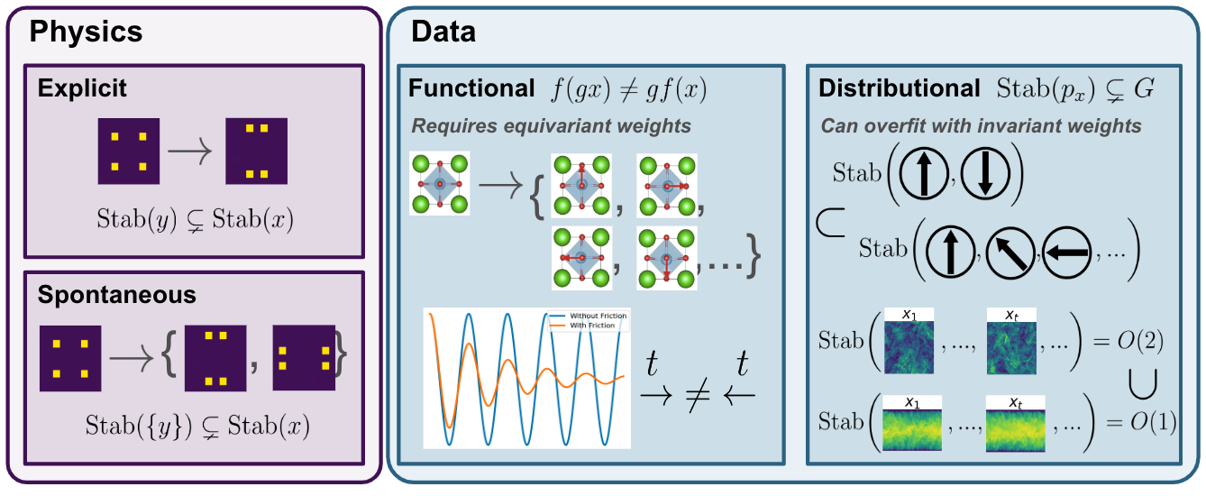
Figure 1: Symmetry breaking can be either explicit, arising when the governing equations are asymmetric, or spontaneous, arising when a symmetric system evolves to a lower symmetry without external influence. It can be also classified as either distributional or functional based on how it manifests in data.

Our method focuses on discovering symmetry-breaking factors from data. The relaxed weights are "analagous" to order parameters used in Landau theory to describe phase transitions (Landau, 1936). Symmetry breaking may arise from: (1) Explicit symmetry breaking: the governing equations of a physical system become variant under the broken symmetry. This could arise from an external force applied to the system or certain boundary conditions. For instance, symmetry-breaking factors, such as gravity, temperature gradient and closed boundaries, break the Euclidean symmetry of a uniform layer of fluid. (2) Spontaneous symmetry breaking: a symmetric system naturally evolves into degenerate lower symmetry states that are energetically favorable without any external symmetry-breaking influence (Castellani & Dardashti, 2021). For example, in the transition of water to ice, the molecules shift from a random, symmetric arrangement in the liquid state to a well-ordered, less symmetric lattice in the solid state.

These forms of symmetry breaking manifest themselves in the data, leading us to categorize potential instances of symmetry breaking as depicted in Figure 1. Assume a function $f:X\mapsto Y$, and $p_{X}:X\mapsto\mathbb{R}$ and $p_{Y}:Y\mapsto\mathbb{R}$ are the probability distributions of the input and output. The expected group $G$ acts on $X$ and $Y$ by $\rho_{X}$ and $\rho_{Y}$.

(1) Single sample symmetry breaking: This could occur when the desired output of the neural network has lower symmetry than the input (e.g. transforming a square to a rectangle). We aim to identify the symmetry operations that differ between the input and output or the “missing information” needed to make the input and output symmetrically compatible. (See (Smidt et al., 2021) for more discussion.). Formally, $\exists\;x\in X,\;\text{Stab}(f(x))\subsetneq\text{Stab}(x)$. Note that this is a special case of (3) below.

(2) Distributional symmetry breaking: In many ideal physical contexts, the entire sample space exhibits symmetry, but a given dataset may or may not. For example, the entire sample space of isotropic flow will be closed under rotations because of the axial symmetry of the flow. Nonetheless, certain boundary conditions and external forces may break this rotational symmetry in a given data distribution $p_{X}$ to varying degrees. Formally, this is stated as $\exists x\in X,\;p_{X}(x)\neq p_{X}(\rho_{X}(g)x)$. Distributional symmetry breaking can be detected by an equivariant model with invariant weights. See Appendix F for more details and examples.

(3) Functional symmetry breaking: the mapping between inputs and outputs is not fully equivariant. For instance, a model with time-reversal equivariance, designed to forecast future states based on historical observations, might have trouble accurately predicting dynamics without time-reversal symmetry, such as processes with increasing entropy (Jucha et al., 2014). Formally, $\exists x\in X\;\text{and}\;\exists g\in G,\;f(\rho_{X}(g)(x))\neq\rho_{Y}(g)f(x)$. Functional symmetry breaking requires equivariant weights to describe.

2.3 Regular Group Convolution

Group convolution (Cohen & Welling, 2016a) achieves equivariance by sharing weights across all group elements. CNNs, for example, achieve shift invariance by implementing group convolution over the group $G=\mathbb{Z}^{2}$ of discrete translations.

Lifting Convolution

The first layer of a $G$-convolutional network typically lifts the input to a function on $G$. It maps the input function $f_{0}$ on $\mathbb{Z}^{3}$ to functions on a group $G=(\mathbb{Z}^{3},+)\rtimes H$, where $H$ is a group acting on $\mathbb{Z}^{3}$ that we desire equivariance with respect to, such as $C_{4}$. The lifting convolution is the same as conventional convolution with a stack of filter banks transformed by the subgroup $H$,

$$(f_{0}\star\psi)(\mathbf{x},h)=\sum_{\mathbf{y}\in\mathbb{Z}^{3}}f_{0}(\mathbf{y})\psi(h^{-1}(\mathbf{y}-\mathbf{x}))$$ (2)

Group Convolution

After the lifting convolution layer, both the filter and input are now functions on $G=(\mathbb{Z}^{3},+)\rtimes H$. A $G$-equivariant group convolution then takes as input a $c_{\mathrm{in}}$-dimensional feature map $f_{1}\colon G\to\mathbb{R}^{c_{\mathrm{in}}}$ and convolves it with kernel $\Psi\colon G\to\mathbb{R}^{c_{\mathrm{out}}\times c_{\mathrm{in}}}$ over a group $G$,

$$(f_{1}\star\Psi)(\mathbf{x},h)=\sum_{\mathbf{y}\in\mathbb{Z}^{3}}\sum_{h^{\prime}\in H}f_{1}(\mathbf{y},h^{\prime})\Psi(h^{-1}(\mathbf{y-x}),h^{-1}h^{\prime})$$ (3)

The last layer usually averages over the $h$-axis and outputs a function on $\mathbb{Z}^{3}$.

2.4 Relaxed Group Convolution

Wang et al. (2022) defines relaxed lifting convolution and relaxed group convolution as below.

Relaxed Lifting Convolution

Unlike a strictly equivariant layer, the relaxed lifting convolution employs additional trainable weights $w_{l}(h)$ and may use several filters $\{\psi_{l}\}_{l=1}^{L}$ instead of one shared filter.

$$(f_{0}\tilde{\star}\psi)(\mathbf{x},h)=\sum_{\mathbf{y}\in\mathbb{Z}^{3}}f(\mathbf{y})\sum_{l=1}^{L}w_{l}(h)\psi_{l}(h^{-1}(\mathbf{y-x}))$$ (4)

The relaxed group convolution weights, transforming as the regular representation of $H$, are the equivariant (non-scalar) weights defined in Section 2.1. The regular representation contains all irreducible representations (irreps) of $H$ as subrepresentations, and thus the relaxed weights can express symmetry breaking corresponding to any irrep.

Relaxed Group Convolution

The group convolution layer is relaxed in the same way.

$$(f_{1}\tilde{\star}\Psi)(\mathbf{x},h)=$$ (5)

$$\sum_{\mathbf{y}\in\mathbb{Z}^{3}}\sum_{h^{\prime}\in H}f_{1}(\mathbf{y},h^{\prime})\sum_{l=1}^{L}w_{l}(h)\Psi_{l}(h^{-1}(\mathbf{y-x}),h^{-1}h^{\prime})$$

Since the weights $\{w_{l}(h)\}$ can vary across group element $h$, this can break the strict weight-sharing scheme. The relaxed weights are (non-scalar) are equivariant weights that transform as the regular representation. We will show that the weights $\{w_{l}(h)\}$ with equal initialization learn to be unequal to break the strict equivariance and adapt to the symmetries of the data when data exhibits broken symmetry.

3 Theoretical Analysis

3.1 Learning symmetry breaking with loss gradients

In the relaxed group convolution, the initial relaxed (equivariant) weights $\{w_{l}(h)\}$ in each layer are set to be the same for all $h$, ensuring that the model exhibits equivariance prior to being trained. In this section, we prove that these relaxed weights only deviate from being equal when the symmetries of the input and the output are lower than that of the model.

Proposition 3.1.

Consider a relaxed group convolutional neural network $f$ where the relaxed weights in each layer are initialized to be identical across group elements to maintain $G$-equivariance. If $f$ is trained to map an input $x$ to output $y$, the relaxed weights will change during training such that $f$ is equivariant to $\text{Stab}(x)\cap\text{Stab}(y)$, which is the intersection of the stabilizers of the input and the output.

In particular, if $\text{Stab}(x)\cap\text{Stab}(y)<G$, then $w_{l}(h)$ will not be constant in $h$ due to the gradients of the loss. The proof can be found in Appendix A. This useful property allows us to discover symmetry or identify symmetry-breaking factors in data because the relaxed weights tell us whether a transformation $h$ stabilizes the input or output. We provide a clear illustration of this through a simple 2D example.

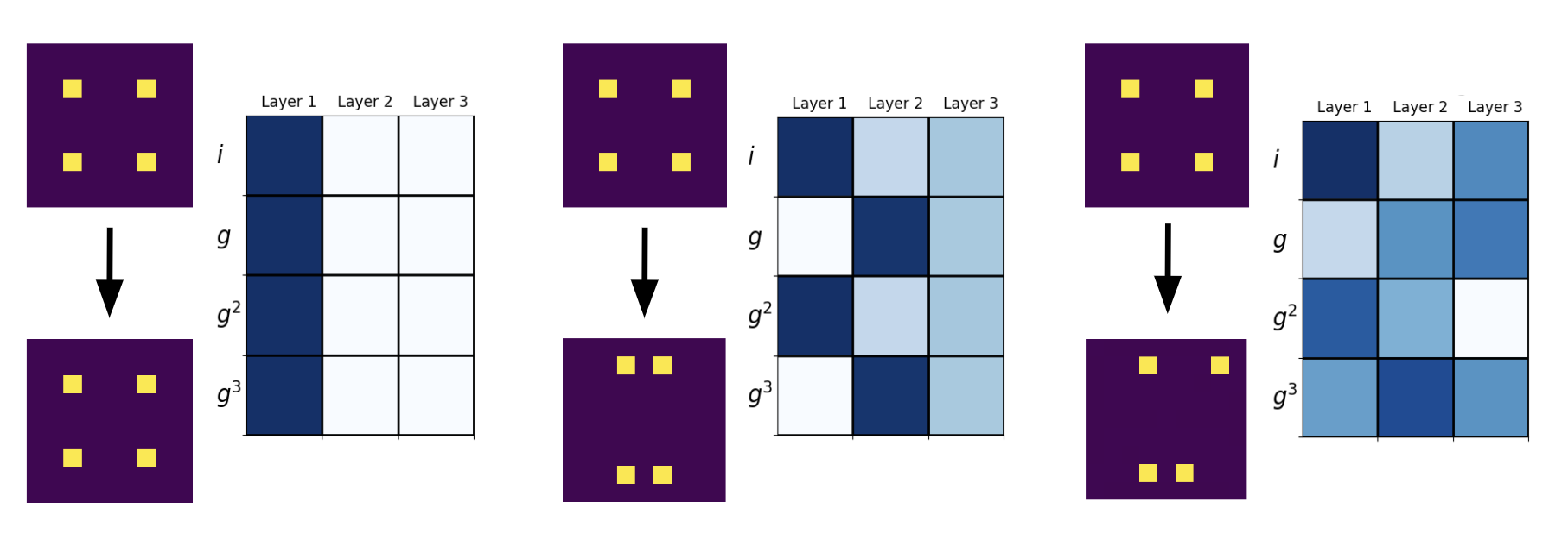
Figure 2: Visualization of tasks and corresponding relaxed weights after training. A 3-layer $C_{4}$-relaxed group convolution network with $L=1$ is trained to perform the following three tasks: 1) map a square to a square; 2) deform a square into a rectangle; 3) map a square to a non-symmetric object.

As shown in Figure 2, in the first task where the output is a square with $C_{4}$ symmetry , relaxed weights across all layers remain equal throughout training. For the second task, where the output is a rectangle exhibiting $C_{2}$ symmetry, the relaxed weights learn to be different. However, the weights corresponding to the group elements $i$ and $g^{2}$ are the same, as are the weights for $g$ and $g^{3}$. This reflects the symmetry of the rectangle as the model becomes equivariant to $C_{2}$ (180 degree rotations). In the final task, where the output lacks any symmetries, the relaxed weights diverge entirely for the four group elements, thereby fully breaking the model’s equivariance.

3.2 Convergence of relaxed weights using mini-batch gradient descent

Proposition 3.1 also indicates that relaxed group convolution can discover symmetries that lie in the data distribution using full batch gradient descent, as the entire dataset can be viewed as a single sample in this case. However, when dealing with high-dimensional data, it often becomes necessary to use mini-batch gradient descent, where mini-batches may not represent the symmetries of the entire dataset. Thus, we have the following proposition.

Proposition 3.2.

Denote $\mu$ the step size of the gradient descent, $M$ the number of mini-batches in each epoch, and $t$ the number of epochs respectively. Assume that the loss function $L$ is convex and has $\delta$-Lipschitz continuous gradients. Consider $\bm{w}^{*}$ the optimal relaxed weights that can be reached by full batch gradient descent, with $K$ representing the gradient noise variance at $\bm{w}^{*}$. Then the starting relaxed weights $\bm{w}^{t}_{0}$ at the $t$-th epoch satisfy

$$E[\|\bm{w}^{t}_{0}-\bm{w}^{*}\|]\leq \left(1-\frac{\mu^{2}\delta^{2}M^{2}}{2\mu^{2}\delta^{2}M^{2}-1}\right)^{t}E[\|\bm{w}^{0}_{0}-\bm{w}^{*}\|]$$

$$+\frac{\mu^{4}\delta^{2}M^{4}K}{1-2\mu^{2}\delta^{2}M^{2}}$$

The convergence rate $1-\frac{\mu^{2}\delta^{2}M^{2}}{2\mu^{2}\delta^{2}M^{2}-1}$ is bounded by $\frac{1}{2}$ and it will descrease as the batch size increases (i.e. $M$ becomes smaller). Given a sufficient number of epochs (i.e. when $t$ is large enough), the relaxed weights learned by mini-batch gradient descent will converge to the optimal relaxed weights learned by the full batch gradient descent. Therefore, training relaxed group convolution with mini-batches still allows for the post-training relaxed weights to uncover the symmetries in the dataset.

3.3 Decomposition of relaxed weights into irreps

By projecting the relaxed weights onto the irreps of the group, similar to calculating its Fourier components, one can identify the type of geometric symmetry breaking and which symmetries are preserved or broken. This is particularly useful for larger groups.

Consider the relaxed weights from a neural network layer illustrated in Figure 2, projected onto $C_{4}$’s four one-dimensional irreps. For the first task, only the Fourier component for the trivial representation is non-zero. In the second task, Fourier components for both the trivial and the sign representation are non-zero, suggesting that either 90 or 180-degree rotational symmetries are broken. Since the remaining irreps are zero, we can conclude the output is still invariant under 180-degree rotations. In the third task, all Fourier components are non-zero. Thus, due to the property that the relaxed group convolution reliably preserves the highest level of equivariance that is consistent with data, it can discover symmetry or symmetry breaking in data.

4 Related Work

4.1 Approximate Symmetry

Equivariant deep learning models have excelled in image analysis(Chidester et al., 2018; Weiler & Cesa, 2019; Kondor & Trivedi, 2018; Bao & Song, 2019; Worrall et al., 2017; Finzi et al., 2020; Ghosh & Gupta, 2019), and their applications have also expanded to physical systems due to the deep relationship between physical symmetries and the principles of physics (Geiger & Smidt, 2022; Wang et al., 2020; Otto et al., 2023; Anderson et al., 2019; Satorras et al., 2021b; Liu et al., 2022; Zitnick et al., 2022; Schütt et al., 2017; Passaro & Zitnick, 2023). However, real-world data rarely conforms to strict mathematical symmetries, due to noise, missing values, or symmetry-breaking features in the underlying physical system. Thus, recent works have tried to relax the strict symmetry constraints imposed on the equivariant networks. Elsayed et al. (2020) first showed that relaxing strict spatial weight sharing in 2D convolution can improve image classification accuracy. Wang et al. (2022) generalized this idea to arbitrary groups and proposed relaxed group convolution, which is biased towards preserving symmetry but is not strictly constrained to do so. Petrache & Trivedi (2023) further provides a theoretical study of how the data equivariance error and the model equivariance error affect the models’ generalization abilities. In this paper, we further apply relaxed group convolution to various physical systems cases and reveal its ability in symmetry discovery. Alternatively, Finzi et al. (2021) proposed a mechanism that sums equivariant and non-equivariant layers but it cannot handle high-dimensional data due to the number of weights in the fully-connected layers. van der Ouderaa et al. (2023) proposed a method to empirically learn the amount of layer-wise equivariance through approximate Bayesian model selection but it does not have theoretical guarantees of learning the correct amount of symmetry from the data. McNeela (2023) proposed the Lie algebra convolution that relaxes the strict equivariance constraints in Lie group convolutions but it cannot be used to find the symmetry-breaking factors.

4.2 Symmetry Discovery

Our method can also perform symmetry discovery as we can uncover hidden symmetries in data by creating relaxed group convolution layers of the largest possible group. This differs from most existing methods for finding symmetries, which often require intricate architecture and careful tuning. For example, Desai et al. (2022); Yang et al. (2023b, a) designed GAN-based architectures where the generator is trained to generate group transformations that stabilize the data distribution. Zhou et al. (2021) factorized the weight matrix into a symmetry matrix, which learns the weight-sharing pattern from the data, and a separate vector for filter parameters. These two parts are trained separately with MAML, which is an optimization-based meta-learning method (Finn et al., 2017). Furthermore, Dehmamy et al. (2021) proposed L-conv, a novel architecture that can learn the Lie algebra basis and automatically discover symmetries from data. Unlike these complex models and training approaches, our method simplifies the process. By utilizing the equivariance property of gradients, the relaxed weights in a single relaxed group convolution layer can discover symmetry breaking with minimal training, either on a single symmetric sample for one iteration or on a symmetric dataset for several epochs.

5 Experiments

5.1 Discovering Symmetry Breaking Factors in Phase Transitions of Crystal Structures

Phase Transition

Modeling a phase transition from a high symmetry (like octahedral) to a lower symmetry is a common topic of interest in materials science (Onuki, 2002). This change can be understood as a transformation in the arrangement or orientation of atoms within a crystal lattice. For instance, perovskite crystal structures consist of connected octahedral motifs that under certain conditions distort and give rise to technologically relevant material properties.

To illustrate, consider the perovskite of Barium Titanate ($BaTiO_{3}$), as shown in Figure 3. At high temperatures, $BaTiO_{3}$ has a cubic perovskite structure with the $Ti$ ion at the center of the octahedron. As one progressively cools $BaTiO_{3}$, it undergoes a series of symmetry-breaking phase transitions. Initially, around 120°C, there is a shift from the cubic phase to a tetragonal phase, where the Ti ion is displaced from its central position. The space group of the tetragonal system in our example is $P4mm$ and the point group is $C_{4v}$. This is followed by a transition to an orthorhombic system at about -90°C, the space group and the point group of which are $Amm2$ and $C_{2v}$ respectively.

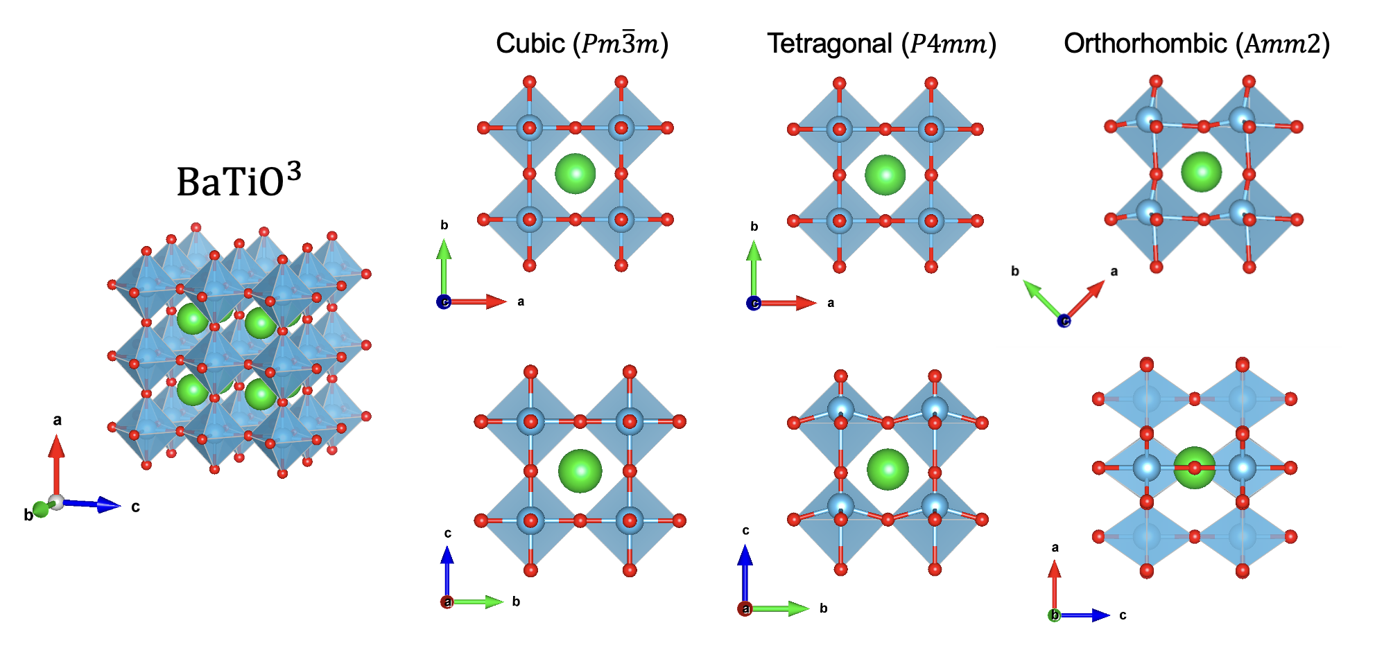
Figure 3: Visualization of $BaTiO_{3}$: As temperature decreases, it undergoes a series of symmetry-breaking phase transitions, transitioning from a cubic structure to a tetragonal phase, and eventually to an orthorhombic form.

Model Design

We build relaxed octahedral group convolution layers to model the phase transition of crystal structures. The octahedral group, denoted $O_{h}$, contains 48 elements. It is a finite subgroup of $O(3)$ that describes all the symmetries of a regular octahedron or a cube. The octahedral group is compatible with the cubic lattice and the highest symmetry group of crystals (Nabarro, 1947; Van der Laan & Kirkman, 1992; Woodward, 1997).

We train a 3-layer relaxed $O_{h}$ group convolutional network with a single filter basis to map from the cubic phase to a tetragonal phase, and from the cubic phase to an orthorhombic system. Since both the input and the network have $O_{h}$ symmetry and the output is lower than $O_{h}$, the post-training relaxed weights reveal the symmetry-breaking factors in these two phase transitions.

Dataset

We use the Cartesian coordinates of $BaTiO_{3}$ in cubic, tetragonal, and orthorhombic phases from the Material Project (Jain et al., 2013). We use 3D tensors to represent these systems where the voxels corresponding to atoms are non-zero. We only focus on the point group symmetry and do not consider translation symmetry breaking in this experiment. Instead, we will explore translation symmetry in the channel flow experiment.

Experimental Results

Figure 4 visualizes the relaxed weights from the two 3-layer models trained to predict the tetragonal and orthorhombic structures from a cubic system. The highlighted relaxed weights are the same as those of the identity element, corresponding to preserved symmetry operations. Since both the input and the model have $O_{h}$ symmetry, based on Theorem 3.1, the highlighted elements stabilize the output of the networks. Those two sets of preserved symmetry operations found by the networks form the $C_{4v}$ and $C_{2v}$ groups respectively, which align with the point group of the tetragonal system ($P4mm$) and the point group of the orthorhombic system ($Amm2$) (Bradley & Cracknell, 2010). These results demonstrate the capability of relaxed group convolution to automatically adapt to the symmetry of the output.

We can further investigate the symmetry-breaking factors by decomposing the relaxed weights that transform under regular representation into the 10 irreducible representations (irreps) of $O_{h}$. The preserved symmetries after phase transitions are the intersection of the stabilizers of all non-zero irreps. More details can be found in Appendix C. As the asymmetry of mapping in this case is due to spontaneous symmetry breaking, to recover all possible configurations, one would need to take the orbit of degenerate solutions.

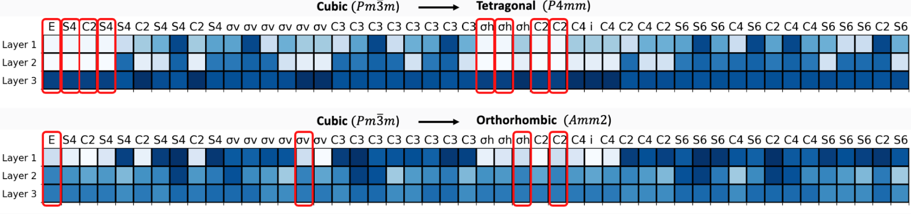
Figure 4: Visualization of the relaxed weights of two 3-layer relaxed octahedral group convolution networks trained to map from the cubic system to the tetragonal system and the orthorhombic system. The highlighted relaxed weights correspond to the preserved symmetry operations in these two systems that forms $C_{4v}$ and $C_{2v}$ group respectively.

5.2 Discovering Isotropy Breaking in Turbulence

Isotropy Breaking

Kolmogorov’s Hypothesis (Zakharov et al., 2012; Pope, 2001) states that, at sufficiently high Reynolds numbers, the small-scale turbulent motions are statistically isotropic and independent of the large-scale structure. This implies that larger eddies lack rotational symmetry due to factors such as boundary conditions and external forces. As they continue to break into smaller eddies and these eddies become sufficiently small, they begin to display rotational symmetries in their distribution. The hypothesis raises the question of determining the specific scale at which fluid symmetries are restored.

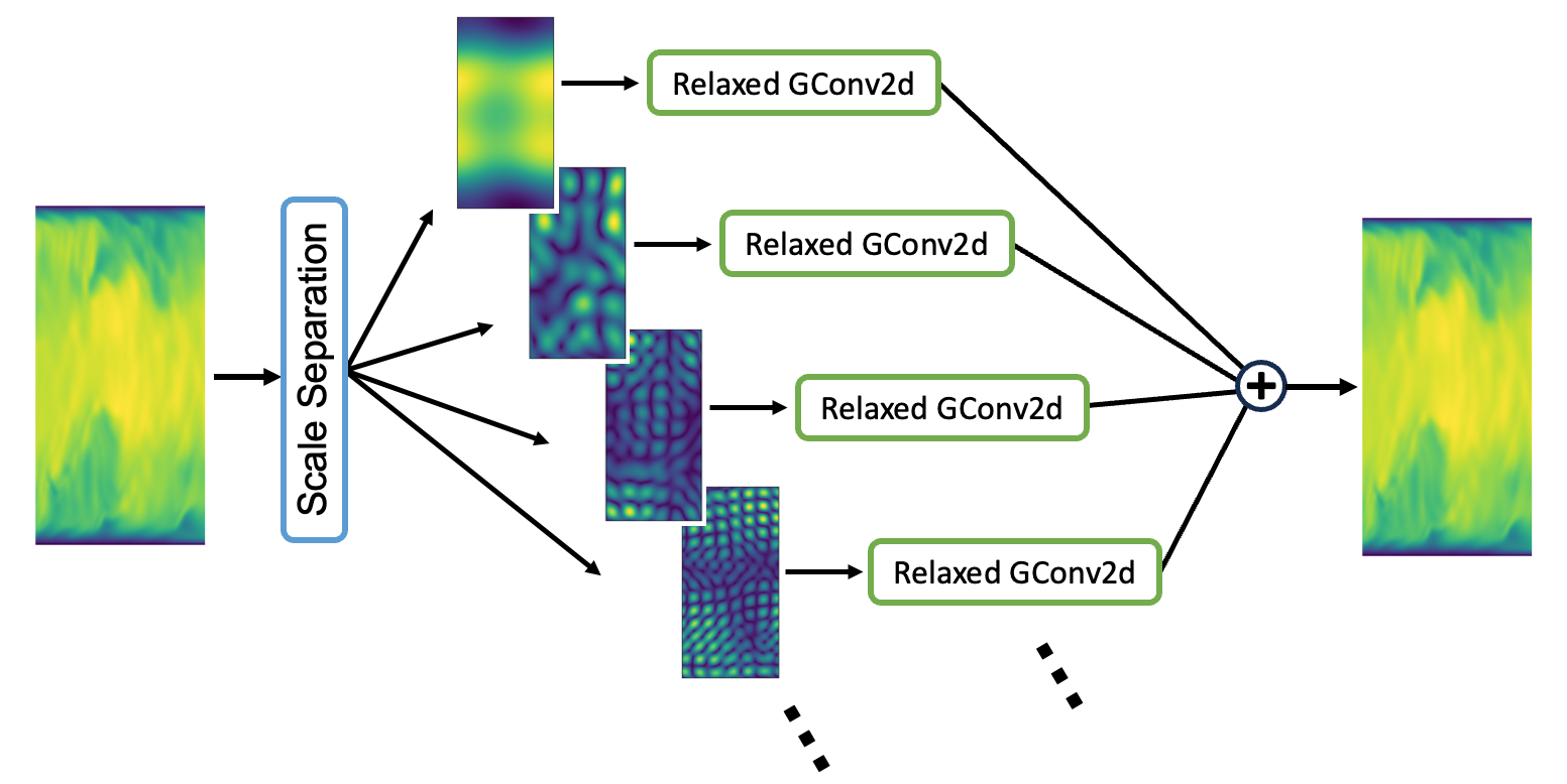
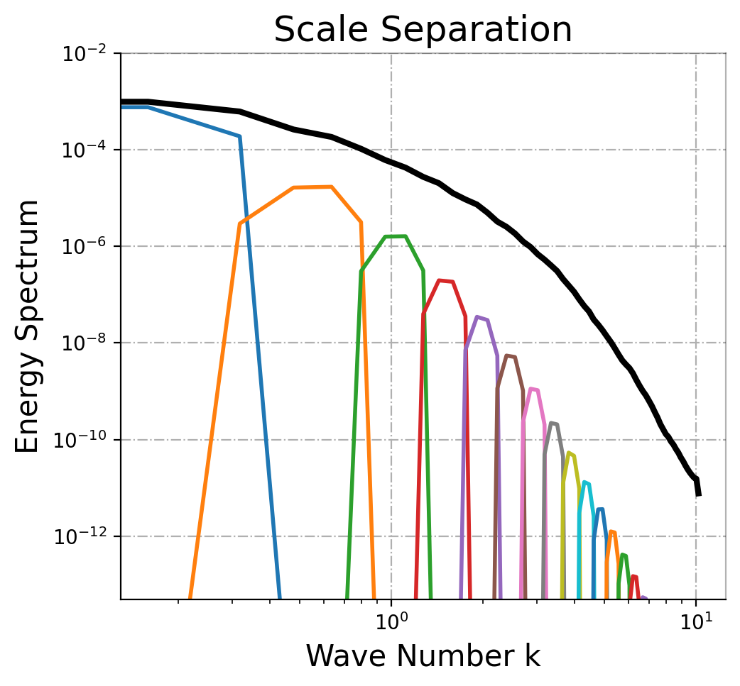
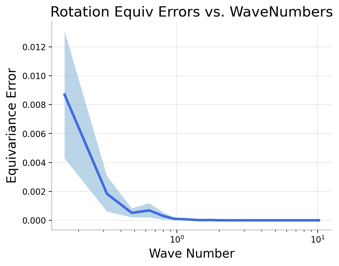
Figure 5: Left: Model for detecting rotational symmetry. This model breaks down the input velocity field into multiple scales using Fourier frequency cutoffs. Each scale is then processed through a distinct relaxed group convolution layer and the sum of the outputs from these layers is trained to reconstruct the input. Middle: Visualization of scale separation in energy spectrum. The black line represents the energy spectrum of the original velocity fields, while the other colored lines correspond to different scales. Right: Equivariance errors learned by the model. As the wave number gets higher (indicating smaller eddies), the equivariance error tends to decrease towards zero, indicating the isotropy crossover point.

Model Design

To identify the symmetries in eddies across various frequencies using relaxed group convolution, it is essential to separate the input velocity fields into different scales. This is achieved by applying different bandpass filters, that is, applying Fourier transformation, frequency cutoff, and inverse Fourier transformation to each frequency range, as illustrated in the left subfigure of Figure 5. The middle subfigure in Figure 5 visualizes the scale separation in the energy spectrum. The black line represents the energy spectrum of the original velocity fields, while the other colored lines correspond to different scales. The turbulence energy spectrum is a quantitative representation of the distribution of kinetic energy across different scales or frequencies of turbulence in a fluid. It characterizes how energy in large eddies transformed into small ones. More details about the energy spectrum are in Appendix D

After scale separation, each scale is then processed through a distinct relaxed group convolution layer. The sum of the outputs from these layers is trained to reconstruct the input. By examining the relaxed weights in the layer corresponding to each scale, the degree of symmetry present at each scale can be determined. We define the equivariance error of a relaxed group convolution layer $f:X\mapsto Y$ as follows,

$$\|f\|_{\text{EE}}=\frac{1}{L|G|}\sum_{l=1}^{L}\sum_{g\in G}\|w_{l}(g)-w_{l}(e)\|$$ (6)

where $G$ is the relevant group ($G$ is $C_{8}$ in this experiment), $L$ is the number of filter banks used in the layer, and $e$ is the identity element in the group $G$. Since $\{w_{l}(g)\}_{g\in G}$ are initialized as equal, $\|f\|_{\text{EE}}$ is zero before training. The bigger $\|f\|_{\text{EE}}$ is after training, the more symmetry breaking there is in the data. Note that the magnitude of relaxed weights is affected by the magnitude of the input. Therefore, the relaxed weights need to be normalized at each scale prior to computing equivariance errors and making comparisons.

Dataset

We use a 2D direct numerical simulation of a turbulent boundary layer flow/channel flow from Gao et al. (2023), which includes a 2000-step simulation of the velocity field at a resolution of 128 x 256. In this dataset, the fluid flows from left to right, bounded by closed boundaries at the top and bottom, as shown in Figure 5. Note that while individual velocity frames do not exhibit symmetry, the entire data distribution may have symmetry. This differs from the earlier example with crystals. In this experiment, our objective is to uncover the rotational invariance of the distribution of the fluid velocities or, more specifically, to detect the statistical isotropy inherent in turbulence.

Experimental Results

The model is trained to reconstruct each velocity field of the turbulent flow simulation using mini-batch gradient descent. We employ an 80%-20% split for training and validation and use early stopping based on the validation loss. After training, the equivariance error for each relaxed group convolution layer is calculated based on Eqn.(6) to obtain the degree of symmetry breaking at different scales. As shown in the right subfigure in Figure 5, as the wavenumber increases (i.e. eddies become smaller), the equivariance errors decrease and approach zero. This implies that the smaller eddies have perfect rotation symmetry, thus empirically validating the Kolmogorov Hypothesis!

Notably, since we use properties of the gradient to discover symmetry, the choice of hyperparameters and the prediction performance of the models do not influence this symmetry-breaking result.

5.3 Discovering Homogeneity Breaking in Turbulence

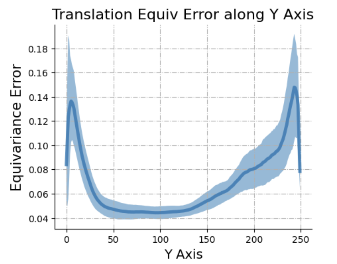
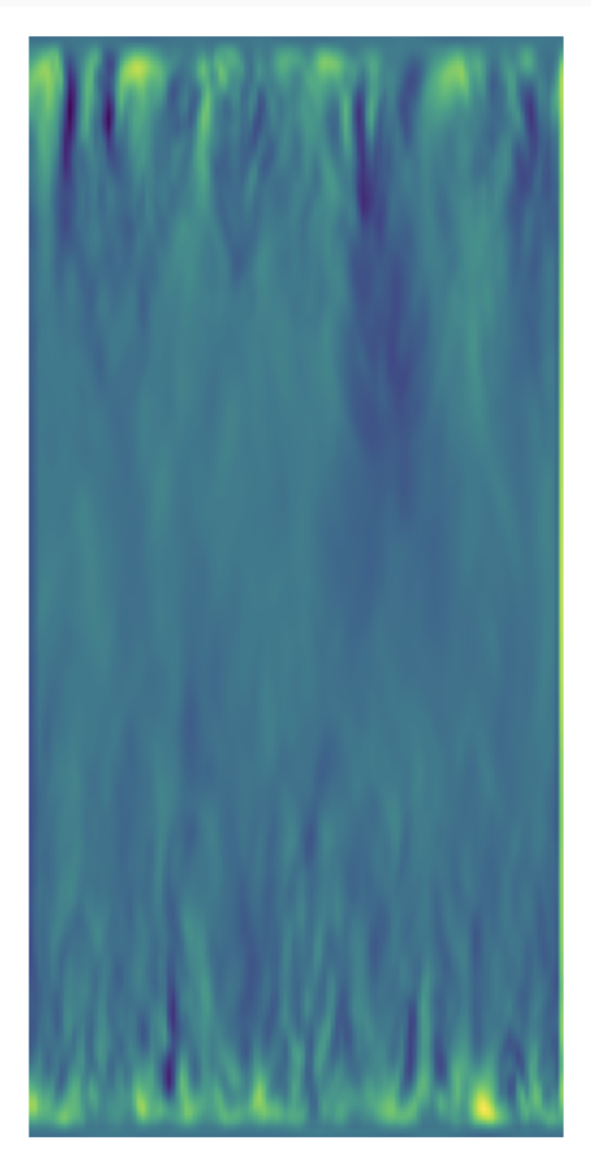
Figure 6: Left: Translation equivariance error along the Y-axis. The level of symmetry breaking increases near the top and bottom boundaries. Right: The visualization of translation relaxed weights. It shows increased variation in relaxed weights as they approach the boundary areas.

Homogeneity Breaking

The turbulence in idealized scenarios is also homogeneous, which means the time-averaged properties of the flow are uniform and independent of position (Wang et al., 2020; Batchelor, 1953). This implies that the distribution of homogeneous turbulence exhibits translation symmetry. Nevertheless, factors like noise and boundary conditions may break this translation symmetry to varying degrees. We will show that the positions of translation symmetry breaking can also be uncovered by the relaxed translation group convolution.

Model Design

The relaxed translation group convolution layer relaxes the translation symmetry by assigning an additional trainable parameter to each spatial position of the input such that every input position does not necessarily share the same convolution kernel. We use the same channel flow dataset and simply train a 3-layer relaxed translation convolution neural network to map each velocity field to itself. The resolution of the simulation of 256$\times$128.

Experimental Results

In Figure 6, the right subfigure is the heatmap of translation relaxed weights of the first layer of the model. We can see the increased variation in relaxed weights as they approach the top and bottom boundaries. We can calculate the equivariance error along the vertical or Y-axis using Eqn. (6), then we can find out how much translation symmetry is broken at different heights. The left subfigure in Figure 6 shows the translation equivariance error along the Y-axis. We can see that the level of symmetry breaking increases near the top and bottom boundaries.

During simulations, perturbation is introduced into the boundaries of simulations to replicate real-world disturbances, which primarily contribute to turbulence. Thus, the translation symmetry or the homogeneity of the fluid is expected to mostly be broken around the boundary regions. This aligns precisely with our findings from the weights of the relaxed translation group convolution networks. The reason why Figure 6 is not perfectly symmetric along the y-axis is that the simulation is not long enough to encompass all possible samples.

Notably, this experiment further demonstrates relaxed group convolution can parameterized to be sensitive not solely to global symmetry breaking but also local symmetry breaking.

5.4 Discovering Time Reversal Symmetry Breaking

Time Reversal Symmetry Breaking

Time reversal symmetry (Lamb & Roberts, 1998) holds for physical laws that remain unchanged when the direction of time is reversed. This symmetry is a key aspect in theoretical physics and has profound implications in various fields such as quantum mechanics, statistical mechanics, and thermodynamics. But not all physical processes exhibit time-reversal symmetry, such as processes that involve entropy increase (Luke et al., 1998; Jucha et al., 2014).

A straightforward example is a pendulum’s motion. Figure 7 visualizes the pendulum simulations without and with friction. In an ideal, frictionless environment, a pendulum swinging back and forth demonstrates time-reversal symmetry. Its motion looks natural and consistent whether viewed normally or in reverse. However, when friction is introduced, this symmetry breaks. Friction causes the pendulum to lose energy and eventually stop. This process would not look the same if time were reversed. This illustrates how time reversal symmetry can be present in idealized systems but is often broken in real-world scenarios with dissipative forces like friction.

Model Design

Since we want to discover time-reversal symmetry, we have developed a one-dimensional relaxed group convolution model that maintains equivariance with the reflection $\{+1,-1\}$ w.r.t the time dimension. Thus, every layer only contains two scalar relaxed weights if we only use a single filter basis (i.e. $L=1$). If these two weights differ after training, it would suggest a break in the symmetry of time reversibility. To test this, we employed a three-layer network adapted for relaxed time reflection group convolution, aiming to predict the pendulum’s angle variations over time. Both the input and the output contain multiple frames.

Dataset

Relaxed time reflection group convolution networks were trained using simulations of pendulum systems initialized at various initial angles. Each simulation trajectory is sliced and follows the standard preprocessing procedure for time series predictions (Benidis et al., 2022).

Experimental Results

We compare the relaxed time reflection weights from models trained on the simulations without and with frictions. As shown in Figure 7, we can see the relaxed weights stay the same across all three layers when the model is trained on frictionless simulations. In contrast, these weights vary when the models are trained on simulations with frictions. These boxplots are based on 10 runs with different random seeds. This result demonstrates the capability of relaxed group convolution in identifying time-reversal symmetry.

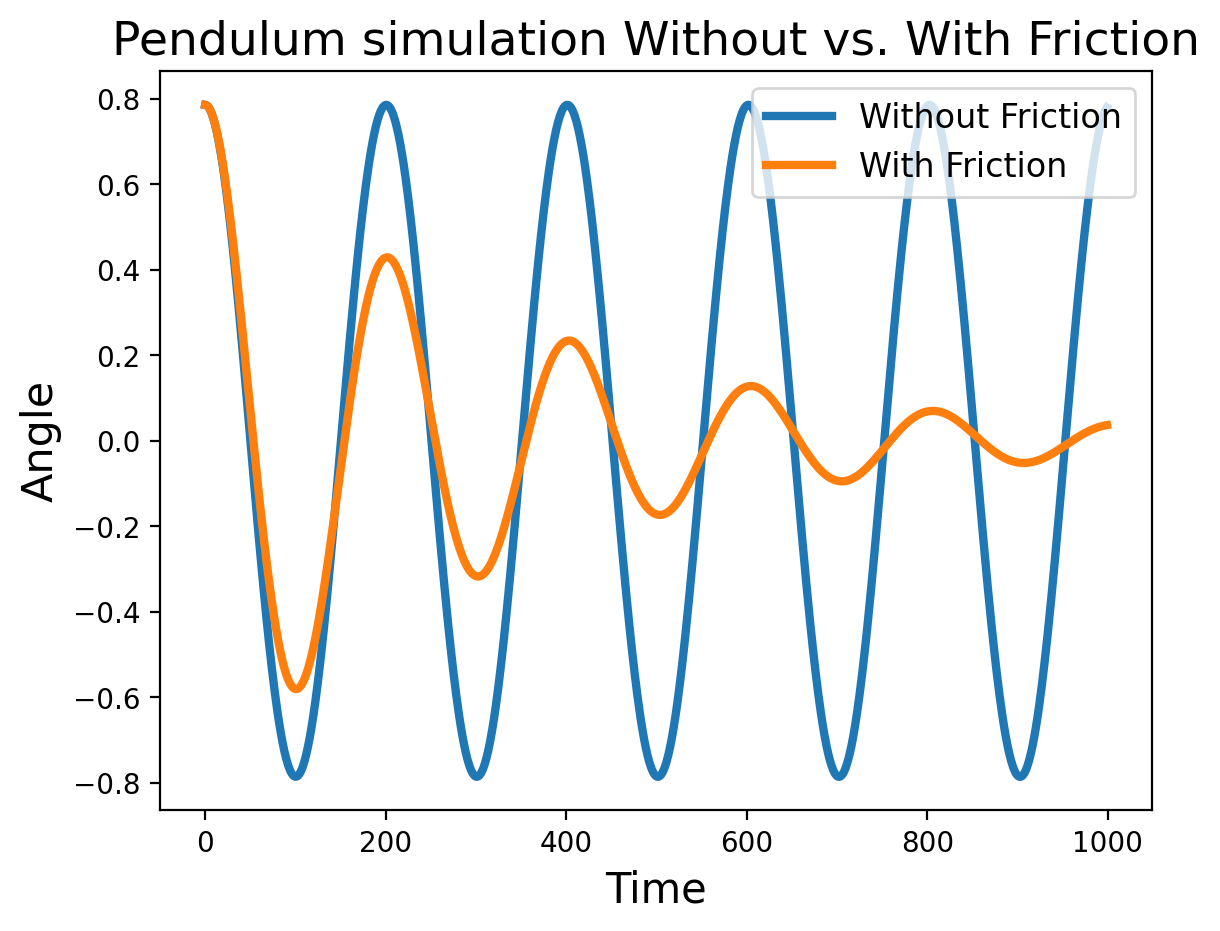
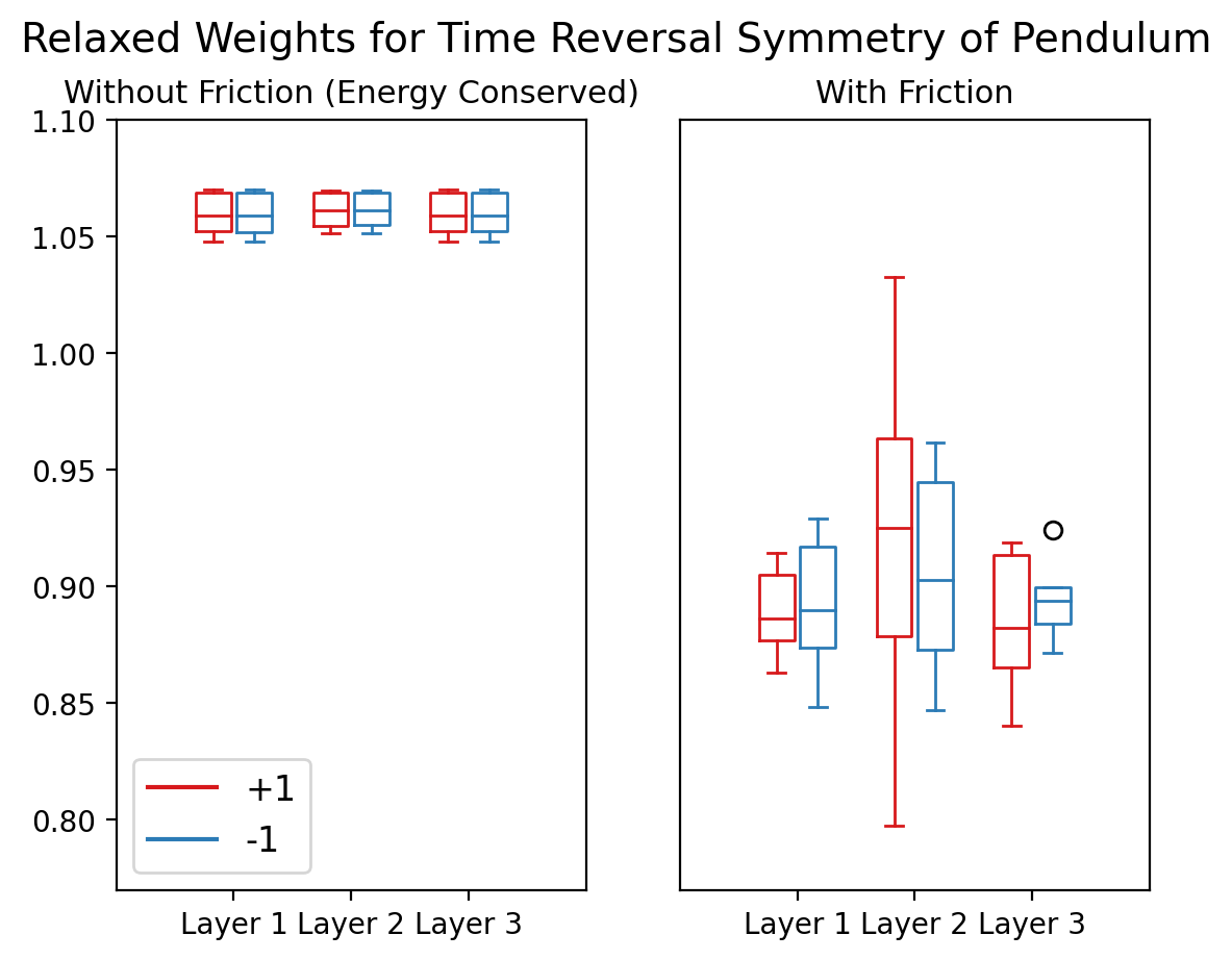
Figure 7: Left: Visualization of the pendulum simulations without and with frictions. Right: the relaxed weights for time reflection from models trained on simulations without and with frictions.

5.5 Super-resolution of 3D Turbulence

We also evaluate the performance of regular, group equivariant, and relaxed group equivariant layers built into this architecture in the tasks of upscaling 3d channel flow and isotropic turbulence. We observe that imposing relaxed equivariance consistently yields better prediction performance. More importantly, Figure 9 in the appendix shows that for isotropic flow, the relaxed weights remain nearly constant across group elements, aligning with its rotational symmetries. Channel flow, on the other hand, is driven by pressure differentials and wall interactions, which makes the turbulence inherently anisotropic. In such cases, the relaxed group convolution is preferable, as it adeptly balances between upholding symmetry principles and adapting to asymmetric factors. All details are in Appendix B.

6 Discussion

We theoretically show and empirically demonstrate that relaxed group convolution adapts to the highest level of equivariance that is consistent with the data distribution and find that the relaxed weights post-training uncover symmetry-breaking factors. We employ various relaxed group convolution architectures to uncover symmetry-breaking factors in different physical systems, including the phase transition of crystal structure, the isotropy and homogeneity breaking in turbulence, and the time-reversal symmetry breaking in pendulum systems.

Our method can also perform symmetry discovery as we can uncover hidden symmetries in data by creating relaxed group convolution layers of the largest possible group. Thus, we include a discussion and experimental results regarding symmetry discovery baselines in Appendix E. Future work includes generalizing the proposed method to graph neural nets and investigating the benefits of relaxed weights in optimization.

Appendix

Appendix A Theoretical Analysis

Proposition A.1.

Consider a relaxed group convolutional neural network $f$ where the relaxed weights in each layer are initialized to be identical across group elements to maintain $G$-equivariance. If $f$ is trained to map an input $x$ to output $y$, the relaxed weights will change during training such that $f$ is equivariant to $\text{Stab}(x)\cap\text{Stab}(y)$, which is the intersection of the stabilizers of the input and the output.

Proof.

Let $G$ be the semi-direct product of the translation group $(\mathbb{Z}^{3},+)$ and a group $H$. Without loss of the generality, we only consider the composition of one lift convolution layer and a relaxed group convolution layer with a single filter bank case (i.e. $L=1$). Suppose the input is $f_{0}(\bm{x})$ and $\phi$ is an unconstrained kernel, then the output of the lift convolution layer is:

$$f_{1}(\bm{y},h)=\sum_{\bm{x}\in\mathbb{Z}^{3}}f_{0}(\bm{x})\phi(h^{-1}(\bm{x}-\bm{y})),\;\;h\in G$$

Now we prove that $f_{1}(\bm{y},h)=f_{1}(k\bm{y},kh),\;k\in G$ only when $k$ stabilizes $f_{0}$.

$$f_{1}(k\bm{y},kh) =\sum_{\bm{x}\in\mathbb{Z}^{3}}f_{0}(\bm{x})\phi((kh)^{-1}(\bm{x}-k\bm{y}))$$

$$=\sum_{\bm{x}\in\mathbb{Z}^{3}}f_{0}(\bm{x})\phi(h^{-1}(k^{-1}\bm{x}-\bm{y}))$$

$$=\sum_{k\bm{x}\in\mathbb{Z}^{3}}f_{0}(k\bm{x})\phi(h^{-1}(\bm{x}-\bm{y}))$$

Thus, $f_{1}(\bm{y},h)=f_{1}(k\bm{y},kh)$ only when $f_{0}(k\bm{x})=f_{0}(\bm{x})$.

We denote $f_{2}(\bm{z},k)$ as the output of the group convolution layer and $\psi$ as the kernel.

$$f_{2}(\bm{z},k)=\sum_{\bm{y}\in\mathbb{Z}^{3}}\sum_{h\in G}f_{1}(\bm{y},h)\psi(k^{-1}(\bm{y}-\bm{z}),k^{-1}h)$$

Now we prove that, $f_{2}(g\bm{z},g)=f_{2}(\bm{z},e),\;g\in G$ only when $g$ stabilizes $f_{0}$, where $e$ is the identity.

$$f_{2}(g\bm{z},g) =\sum_{\bm{y}\in\mathbb{Z}^{3}}\sum_{h\in G}f_{1}(\bm{y},h)\psi(g^{-1}(\bm{y}-g\bm{z}),g^{-1}h)$$

$$=\sum_{g\bm{y}\in\mathbb{Z}^{3}}\sum_{gh\in G}f_{1}(g\bm{y},gh)\psi(\bm{y}-\bm{z}),h)$$

Thus, $f_{2}(g\bm{z},g)=f_{2}(\bm{z},e)$ only when $f_{1}(g\bm{y},gh)=f_{1}(\bm{y},h)$, which means $f_{0}$ needs to be stablized by $g$ given the previous step of the proof.

Let $Y(\bm{z})$ and $\hat{Y}(\bm{z})$, $\bm{z}\in\mathbb{Z}^{3}$, be the target and prediction respectively and $L$ is MSE loss. In the last layer, we usually average over the $H$-axis and we can define $\hat{Y}(\bm{x})$ based on the definition of relaxed group convolution as follows:

$$\hat{Y}(\bm{z})=\sum_{k\in H}w(k)f_{2}(\bm{z},k)$$

where $w(k)$ are the relaxed weights. We use MSE loss:

$$L=\sum_{\bm{z}\in\mathbb{Z}^{3}}(Y(\bm{z})-\hat{Y}(\bm{z}))^{2}$$

Finally, we can compute the gradient of the loss $L$ w.r.t a relaxed weight $w(k)$:

$$\frac{\partial L}{\partial w(k)} =\sum_{\bm{z}\in\mathbb{Z}^{3}}\frac{\partial L}{\partial\hat{Y}(\bm{z})}\frac{\partial\hat{Y}(\bm{z})}{\partial w(k)}$$

$$=-2\sum_{\bm{z}\in\mathbb{Z}^{3}}|Y(\bm{z})-\sum_{t\in H}f_{2}(\bm{z},t)|f_{2}(\bm{z},k)$$

$$=-2\sum_{k\bm{z}\in\mathbb{Z}^{3}}|Y(k\bm{z})-\sum_{t\in H}f_{2}(k\bm{z},t)|f_{2}(k\bm{z},k)$$

This means if $k$ does not stabilize the input $f_{0}$, then $f_{2}(\bm{kz},k)\neq f_{2}(\bm{z},e)$, i.e. $\frac{\partial L}{\partial w(k)}\neq\frac{\partial L}{\partial w(e)}$

If $k$ stabilizes the input $f_{0}$, then

$$\frac{\partial L}{\partial w(k)} =-2\sum_{k\bm{z}\in\mathbb{Z}^{3}}(Y(k\bm{z})-\sum_{t\in H}f_{2}(\bm{z},k^{-1}t))f_{2}(\bm{z},e)$$

$$=-2\sum_{\bm{z}\in\mathbb{Z}^{3}}(Y(k\bm{z})-\sum_{t\in H}f_{2}(\bm{z},t))f_{2}(\bm{z},e)$$

Then we can see $\frac{\partial L}{\partial w(k)}=\frac{\partial L}{\partial w(e)}$ only when $Y(k\bm{z})=Y(\bm{z})$.

In conclusion, $\frac{\partial L}{\partial w(k)}=\frac{\partial L}{\partial w(e)}$ only when $k$ stabilizes both the input $f_{0}$ and the target $Y$. ∎

Proposition A.2.

Denote $\mu$ as the step size of the gradient descent, $M$ as the number of mini-batches in each epoch, and $t$ as the number of epochs respectively. Assume that the loss function $L$ is convex and has $\delta$-Liptischitz continuous gradients. Consider $\bm{w}^{*}$ as the optimal relaxed weights that can be reached by full batch gradient descent, with $K$ representing the gradient noise variance at $\bm{w}^{*}$. Then the starting relaxed weights $\bm{w}^{t}_{0}$ at the $t$-th epoch satisfies

$$E\|\bm{w}^{t}_{0}-\bm{w}^{*}\|\leq(\frac{\mu^{2}\delta^{2}M^{2}-1}{2\mu^{2}\delta^{2}M^{2}-1})^{t}E\|\bm{w}^{0}_{0}-\bm{w}^{*}\|+\frac{\mu^{4}\delta^{2}M^{4}K}{1-2\mu^{2}\delta^{2}M^{2}}$$

Proof.

Denote $\mu$ as the step size of the gradient descent, $M$ as the number of mini-batches in each epoch, , $t$ as the number of epochs, $B$ as the batch size, and $N$ as the total number of training samples. Let $z_{i}=\{(x_{j},y_{j})\}_{j=B*i}^{B*(i+1)}$ be a mini-batch of training samples. The optimal relaxed weights $\bm{w}^{*}$ can be defined as

$$\bm{w}^{*}=\text{argmin}J(\bm{w})=\text{argmin}\frac{1}{M}\sum_{i=1}^{M}L(\bm{w};z_{i})$$

Assumption 1: we assume that $L(\bm{w};z)$ is differentiable and has $\delta$-Liptischitz continous gradients, i.e.

$$\|\nabla_{\bm{w}}L(\bm{w}_{1};z_{i})-\nabla_{\bm{w}}L(\bm{w}_{2};z_{i})\|\leq\delta\|\bm{w}_{1}-\bm{w}_{2}\|,\;\;i=1,...,M$$

Assumption 2: we assume $J(\bm{w})$ is convex, for any $\bm{w}_{1},\bm{w}_{2}$:

$$(J_{\bm{w}_{1}}(\bm{w}_{1})-J_{\bm{w}_{2}}(\bm{w}_{2}))^{T}(\bm{w}_{1}-\bm{w}_{2})\geq 0$$

We denote $\bm{w}_{i}^{t}$ as the relaxed weights at iteration $i$ in $t$-th epoch. That means,

$$\bm{w}_{i}^{t}=\bm{w}_{i-1}^{t}-\mu\nabla_{\bm{w}}L(\bm{w}_{i-1}^{t},z_{i}^{t})$$

$$\bm{w}_{0}^{t+1}=\bm{w}_{M}^{t} =\bm{w}_{M-1}^{t}-\mu\nabla_{\bm{w}}L(\bm{w}_{M-1}^{t},z_{M}^{t})$$

$$=\bm{w}_{0}^{t}-\mu\sum_{i=1}^{M}\nabla_{\bm{w}}L(\bm{w}_{i-1}^{t},z_{i}^{t})$$

$$=\bm{w}_{0}^{t}-\mu M\nabla_{\bm{w}}J(\bm{w}_{0}^{k})-\mu\sum_{i=1}^{M}[\nabla_{\bm{w}}L(\bm{w}_{i-1}^{t},z_{i}^{t})-\nabla_{\bm{w}}L(\bm{w}_{0}^{t},z_{i}^{t})]$$

We denote the last term $\sum_{i=1}^{M}[\nabla_{\bm{w}}L(\bm{w}_{i-1}^{t},z_{i}^{t})-\nabla_{\bm{w}}L(\bm{w}_{0}^{t},z_{i}^{t})]$ as $\epsilon_{i}^{t}(\bm{w}_{i-1}^{t})$, which is the gradient mismatch between using mini-batch gradient descent and full batch gradient descent.

Let $\tilde{\bm{w}}_{0}^{t}=\bm{w}^{*}-\bm{w}^{t}_{0}$ and subtract $\bm{w}^{*}$ from both sides,

$$\|\tilde{\bm{w}}_{0}^{t+1}\|^{2} =\|\tilde{\bm{w}}_{0}^{t}+\mu M\nabla_{\bm{w}}J(\bm{w}_{0}^{t})+\mu\sum_{i=1}^{M}\epsilon_{i}^{t}(\bm{w}_{i-1}^{t})\|^{2}$$

$$\leq\|\tilde{\bm{w}}_{0}^{t}+\mu M\nabla_{\bm{w}}J(\bm{w}_{0}^{t})\|^{2}+\|\mu\sum_{i=1}^{M}\epsilon_{i}^{t}(\bm{w}_{i-1}^{t})\|^{2}$$

$$\leq\|\tilde{\bm{w}}_{0}^{t}+\mu M\nabla_{\bm{w}}J(\bm{w}_{0}^{t})\|^{2}+\mu^{2}M\sum_{i=1}^{M}\|\epsilon_{i}^{t}(\bm{w}_{i-1}^{t})\|^{2}$$

For the first term, we have

$$\|\tilde{\bm{w}}_{0}^{t}+\mu M\nabla_{\bm{w}}J(\bm{w}_{0}^{t})\|^{2} =\|\tilde{\bm{w}}_{0}^{t}\|^{2}+\mu^{2}M^{2}\|\nabla_{\bm{w}}J(\bm{w}_{0}^{t})\|^{2}+2\mu M(\tilde{\bm{w}}_{0}^{t})^{T}\nabla_{\bm{w}}J(\bm{w}_{0}^{t})$$

Because of the convexity of $J$, we have

$$(\tilde{\bm{w}}_{0}^{t})^{T}\nabla_{\bm{w}}J(\bm{w}_{0}^{t})=(\bm{w}^{*}-\bm{w}_{0}^{t})^{T}(\nabla_{\bm{w}}J(\bm{w}_{0}^{t})-\nabla_{\bm{w}}J(\bm{w}^{*}))=-(\bm{w}_{0}^{t}-\bm{w}^{*})^{T}(\nabla_{\bm{w}}J(\bm{w}_{0}^{t})-\nabla_{\bm{w}}J(\bm{w}^{*}))\leq 0$$

Because $L$ has $\delta$-Liptischitz continuous gradients, we have

$$\|\nabla_{\bm{w}}J(\bm{w}_{0}^{t})\|^{2}=\|\nabla_{\bm{w}}J(\bm{w}_{0}^{t})-\nabla_{\bm{w}}J(\bm{w}^{*})\|^{2}\leq\delta\|\bm{w}_{0}^{t}-\bm{w}^{*}\|^{2}=\delta^{2}\|\tilde{\bm{w}}_{0}^{t}\|^{2}$$

For the second term $\sum_{i=1}^{M}\|\epsilon_{i}^{t}(\bm{w}_{i-1}^{t})\|^{2}$, we can directly use the result in the Appendix B in Ying et al. (2018),

$$\sum_{i=1}^{M}\|\epsilon_{i}^{t}(\bm{w}_{i-1}^{t})\|^{2}\leq\frac{\mu^{2}\delta^{2}M^{3}}{1-\mu^{2}\delta^{2}M^{2}}(2\delta^{2}\|\tilde{\bm{w}}_{0}^{t}\|^{2}+K)$$

where $K=\frac{1}{M}\sum_{i=1}^{M}\|\nabla_{\bm{w}}L(\bm{w}^{*},z_{i})\|^{2}$. It is the gradient noise variance at optimal point $\bm{w}^{*}$.

Thus,

$$\|\tilde{\bm{w}}_{0}^{t+1}\|^{2}\leq\frac{\mu^{2}\delta^{2}M^{2}-1}{2\mu^{2}\delta^{2}M^{2}-1}\|\tilde{\bm{w}}^{t}_{0}\|^{2}+\frac{\mu^{4}\delta^{2}M^{4}K}{1-2\mu^{2}\delta^{2}M^{2}}$$

Iterating over $t$, we have

$$\|\tilde{\bm{w}}_{0}^{t+1}\|^{2} \leq(\frac{\mu^{2}\delta^{2}M^{2}-1}{2\mu^{2}\delta^{2}M^{2}-1})^{t}\|\tilde{\bm{w}}^{0}_{0}\|^{2}+(\frac{\mu^{4}\delta^{2}M^{4}K}{1-2\mu^{2}\delta^{2}M^{2}})\sum_{j=1}^{t}(\frac{\mu^{2}\delta^{2}M^{2}-1}{2\mu^{2}\delta^{2}M^{2}-1})^{j}$$

$$\leq(\frac{\mu^{2}\delta^{2}M^{2}-1}{2\mu^{2}\delta^{2}M^{2}-1})^{t}\|\tilde{\bm{w}}^{0}_{0}\|^{2}+(\frac{\mu^{4}\delta^{2}M^{4}K}{1-2\mu^{2}\delta^{2}M^{2}})\sum_{j=1}^{t}(\frac{1}{2})^{j}$$

$$\leq(\frac{\mu^{2}\delta^{2}M^{2}-1}{2\mu^{2}\delta^{2}M^{2}-1})^{t}\|\tilde{\bm{w}}^{0}_{0}\|^{2}+(\frac{\mu^{4}\delta^{2}M^{4}K}{1-2\mu^{2}\delta^{2}M^{2}})$$

$$\leq(1-\frac{\mu^{2}\delta^{2}M^{2}}{2\mu^{2}\delta^{2}M^{2}-1})^{t}\|\tilde{\bm{w}}^{0}_{0}\|^{2}+(\frac{\mu^{4}\delta^{2}M^{4}K}{1-2\mu^{2}\delta^{2}M^{2}})$$

∎

Appendix B Super-resolution of Velocity Fields in Three-dimensional Fluid Dynamics

Data Description.

We use the direct numerical simulation data of the channel flow ($2048\times 512\times 1536$) turbulence and the forced isotropic turbulence ($1024^{3}$) from Johns Hopkins Turbulence Database (Kanov et al., 2015). For each dataset, we acquire 50 frames of velocity fields, which are then downscaled by half and segmented into $64^{3}$ cubes for experimental use. These cubes are further downsampled by a factor of 4 to serve as input for our superresolution model. The models are trained to generate $64^{3}$ simulations from $16^{3}$ downsampled versions of themselves. Because of the spatial weight sharing of CNNs, we can apply our model to 3D input with any resolution during inference.

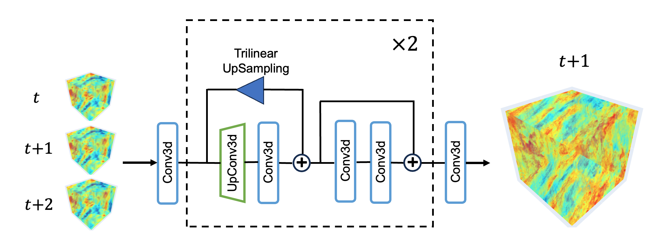
Figure 8: The architecture of the super-resolution model includes an input layer, an output layer, and eight residual blocks. Since it has two layers of Transposed Convolution(UpConv3d), the model produces simulations that are upscaled by a factor of four.

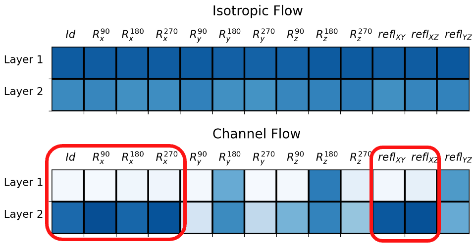
Figure 9: Visualization of the relaxed weights of first two layers from the models trained on the isotropic flow and channel flow.

Table 1: Prediction MAE of trilinear upsampling, non-equivariant, equivariant, relaxed equivariant models on the super-resolution of channel flow and isotropic flow.

	Channel Flow $(10^{-2})$				Isotropic Flow $(10^{-1})$
Model	Trilinear	Conv	Equiv	R-Equiv	Trilinear	Conv	Equiv	R-Equiv
MAE	5.24	2.60$\pm$0.05	2.54$\pm$0.03	$\bm{2.44\pm 0.01}$	5.25	1.22$\pm$0.04	1.12$\pm$0.02	$\bm{1.00\pm 0.01}$

Experimental Setup

Figure 8 visualizes the model architecture we use for super-resolution. We evaluate the performance of Regular, Group Equivariant, and Relaxed Group Equivariant layers built into this architecture in the tasks of upscaling channel flow and isotropic turbulence. The models take three consecutive steps of downsampled $16^{3}$ velocity fields as input and predict a single step of $64^{3}$ simulation, enabling them to infer vital attributes like acceleration and external forces for precise small-scale turbulence predictions. We use the L1 loss function over the L2 loss, as it significantly enhances performance. We split the data 80%-10%-10% for training-validation-test across time and report mean absolute errors over three random runs. As for hyperparameter tuning, except for fixing the number of layers and kernel sizes, we perform a grid search for the learning rate, hidden dimensions, batch size, and the number of filter bases for all three types of models.

Prediction Performance

Table 1 shows the prediction MAE of trilinear upsampling, non-equivariant, equivariant, and relaxed equivariant models applied to super-resolution tasks for both channel and isotropic flows. Figure 10 shows the 2D velocity norm field of predictions. As we can see, imposing equivariance and relaxed equivariance consistently yields better prediction performance. It is fascinating to see that relaxed group convolution performs best even on the isotropic flow, which exhibits distributional rotation symmetry. We conjecture that relaxed weights may also enhance optimization, which we will leave for future work.

Figure 9 visualizes the relaxed weights of the first two layers from the models trained on isotropic flow and channel flow. The relaxed weights for isotropic flow stay almost the same across group elements while those for channel flow vary greatly, which conforms to the symmetries of these two types of flow. For isotropic turbulence, even if individual samples might not seem symmetrical, the statistical properties of their velocity fields over time and space are invariant with respect to rotations. This makes models trained on isotropic flow benefit more from the equivariance.

Channel flow, on the other hand, is driven by a pressure difference between the two ends of the channel together with the walls, which makes the turbulence inherently anisotropic. In such cases, the relaxed group convolution is preferable, as it adeptly balances between upholding certain symmetry principles and adapting to factors that introduce asymmetry. As we can see from the highlighted relaxed weights from Figure 9, though most symmetries are broken, the model can still learn approximate $D_{4}$ symmetry along the direction of the channel flow.

Though group convolution has been a powerful tool for many applications, its computational complexity scales exponentially with the dimensionality of the group, which is the main practical challenge when dealing with the octahedral group. To improve parameter efficiency, we employ separable group convolution that assumes the convolution kernels are separable (Knigge et al., 2022).

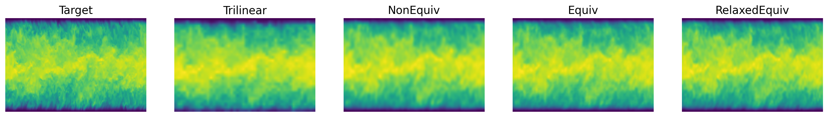
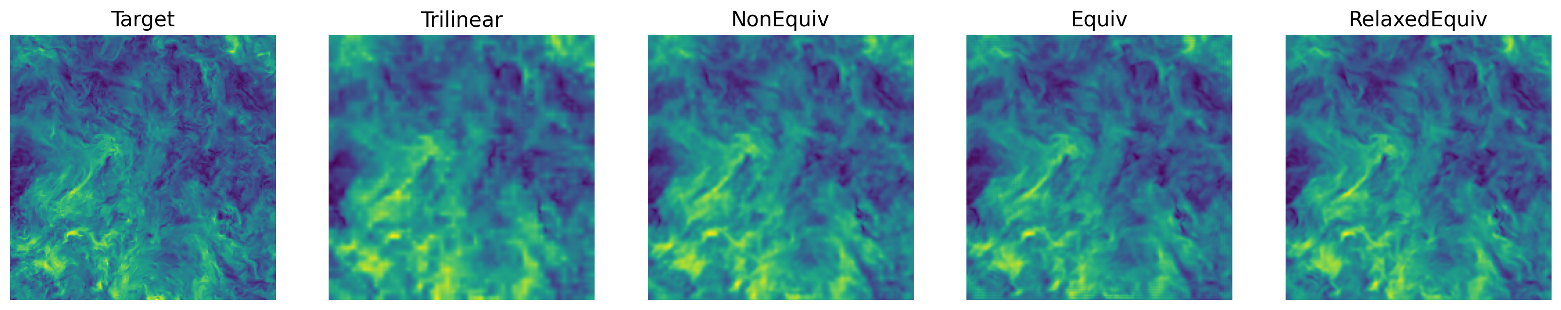
Figure 10: Prediction visualization of a cross-section along the z-axis of the velocity norm fields.

Appendix C Irrep Analysis

Proposition C.1.

Consider a relaxed group convolution neural network for some group $G$ and $w\in\mathbb{R}^{G}$ is the relaxed weights from one of the layers. $w$ transforms under the regular representation $L_{g}\in\mathbb{R}^{G\times G}$ of the group $G$. $\{\rho_{\lambda}\}$ are the set of unique irreducible representations of $G$. The Fourier transform of $w$ at irreducible representation $\rho_{\lambda}$ is defined as: $\hat{w}(\lambda)=\sum_{g}\rho_{\lambda}(g)w(g)$. We also define the stabilizer of $w$ as $\text{Stab}_{G}(w)=\{g|L_{g}w=w\}$ and the stabilizer of $\hat{w}(\lambda)$ as $\text{Stab}_{G}(\hat{w}(\lambda))=\{g|\rho_{\lambda}(g)\hat{w}(\lambda)=\hat{w}(\lambda)\}$. Then the stabilizer of $w$ is the same as the intersection of the stabilizers of the Fourier transforms across all irreducible representations, i.e. $\text{Stab}_{G}(w)=\cap_{\lambda}\text{Stab}_{G}(\hat{w}(\lambda))$.

Proof: The Fourier transform of $w$ on Group $G$, $\mathcal{F}:\mathbb{R}^{G}\rightarrow\bigoplus_{\lambda}\text{End}(V_{\lambda})$, is an isomorphism implied in the Wedderburn theorem and the inverse formula can be defined as:

$$w(g)=\frac{1}{|G|}\sum_{\lambda}d_{\lambda}tr(\hat{w}(\lambda)(\rho_{\lambda}(g))^{-1})$$

where the $V_{\lambda}$ is subspace that $\rho_{\lambda}$ acts on and $d_{\lambda}$ is the dimension of $V_{\lambda}$.

$\mathcal{F}$ is equivariant as well because

$$\rho_{\lambda}(h)\hat{w}(\lambda)=\sum_{g}\rho_{\lambda}(h)\rho_{\lambda}(g)w(g)=\sum_{g}\rho_{\lambda}(hg)w(g)=\sum_{g}\rho_{\lambda}(g)w(h^{-1}g)=\widehat{L_{h}w}(\lambda),\;\;\;\forall\lambda\in G$$

Thus, $\mathcal{F}(L_{h}w)=\bigoplus_{\lambda}\bigoplus_{d_{\lambda}}\rho_{\lambda}(h)vec(\hat{w}(\lambda)),\;\;\forall h\in G$. That means if $w$ is stabilized by $h$, then $h$ stabilizes the Fourier transform across all irreducible representations. The reverse also holds.

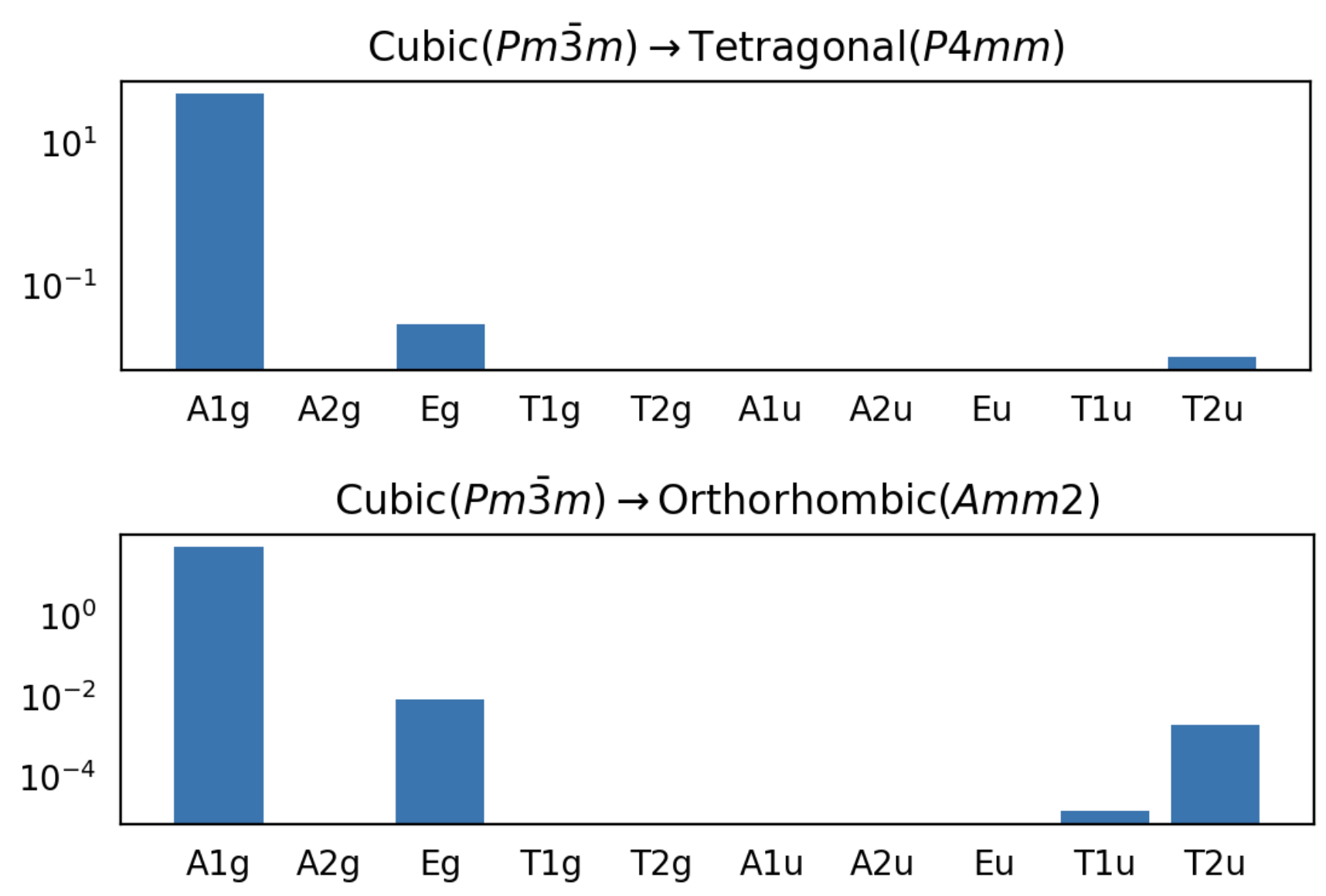
Figure 11: Visualization of the coefficients of 10 irreps of the octahedral group. The symmetries that are preserved after phase transitions are the intersection of the stabilizers of all non-zero irreps.

Appendix D Turbulence kinetic energy spectrum

The turbulence energy spectrum is a concept in fluid dynamics that describes the distribution of kinetic energy among different scales of motion in a turbulent flow. It’s based on the understanding that turbulence comprises a wide range of eddies or vortices of different sizes, each carrying a certain amount of energy. The turbulence kinetic energy spectrum $E(k)$ is related to the mean turbulence kinetic energy as

$$\int_{0}^{\infty}E(k)dk =(\overline{(u^{{}^{\prime}})^{2}}+\overline{(v^{{}^{\prime}})^{2}})/2,$$

$$\overline{(u^{{}^{\prime}})^{2}} =\frac{1}{T}\sum_{t=0}^{T}(u(t)-\bar{u})^{2},$$

where the $k$ is the wavenumber and $t$ is the time step. Figure 12 shows a theoretical turbulence kinetic energy spectrum plot. The spectrum can describe the transfer of energy from large scales of motion to the small scales and provides a representation of the dependence of energy on frequency.

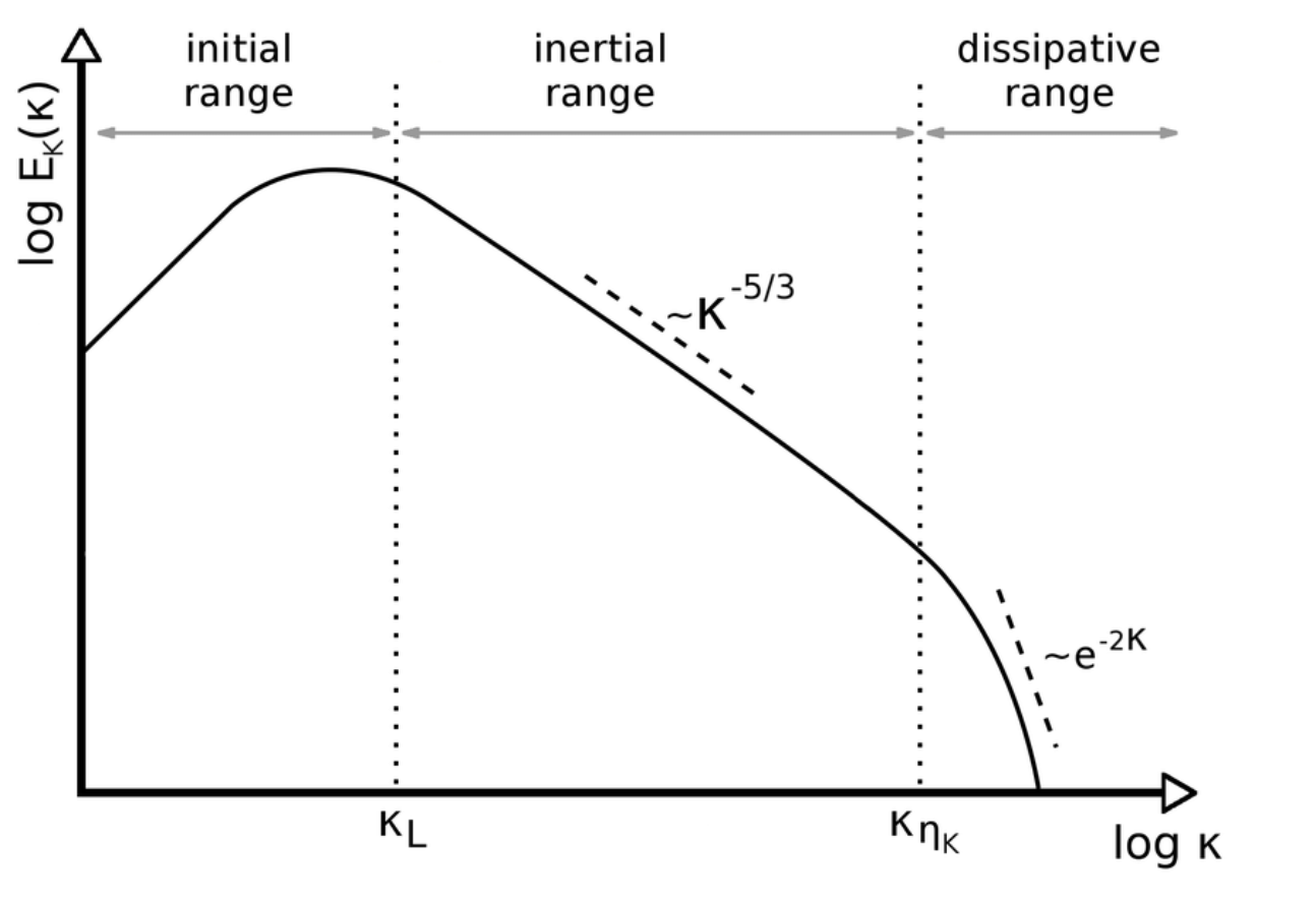
Figure 12: Theoretical turbulence energy spectrum plot: The energy spectrum is often represented graphically, showing energy (usually on a logarithmic scale) as a function of wave number or size of the eddies. In Kolmogorov’s theory, for the inertial subrange (a range of scales where the energy transfer is dominated by inertia forces rather than viscous forces), the energy spectrum follows a -5/3 power law.

Appendix E Comparison to baselines

Comparing our method with other symmetry discovery approaches mentioned in section 4.2 is non-trivial, and these methods fall short of the capabilities demonstrated by our approach for several technical reasons: 1) all of these methods focus on symmetry discovery in the data distribution but lack ability to identify symmetries at the individual sample level; 2) They may only perform well on the datasets with perfect symmetry and lack the quantitative mechanisms to measure the extent of symmetry breaking. 3) They are based on intricate architectures and training strategies and often require careful tuning.

The works most closely related to our study are MSR (Zhou et al., 2021) and LieGAN (Yang et al., 2023b). MSR proposed a method to learn the weight-sharing matrix and the non-constrained filters separately by an optimization-based meta-learning method (Finn et al., 2017). The post-training weight-sharing matrix uncovers the symmetries in the data. We attempted applying MSR to identify rotation and translation symmetries in fluid dynamics. Meanwhile, LieGAN, built on generative adversarial networks, aims to identify the Lie generator of continuous groups from the training data, making it potentially suitable for detecting rotational symmetry in fluid’s small eddies

The MSR approach in (Zhou et al., 2021) is limited to 1D translation convolution models, which cannot be directly applied to our 2D fluid data. Thus, we train a distinct MSR model for each height (i.e. y coordinate). Figure 13 left visualizes the translation weight-sharing matrices learned at different y-coordinates through MSR. As we can see, though the weight-sharing matrices are very noisy, the MSR can find that there is a certain amount of translation symmetry in the data. However, when we measured the equivariance errors (EE) of models at different $y$, the results did not accurately reflect the correct amount of symmetries at different heights as we expected. Additionally, we performed a grid search of hyperparameters but failed to make the MSR to learn the correct rotation symmetry from the fluid data. Figure 13 middle displays the rotation weight-sharing matrices learned by MSR for the C4 group, where ideally, at high frequencies, the matrix should be a stack of permutation matrices.

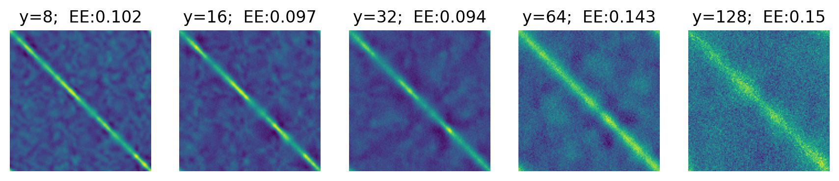
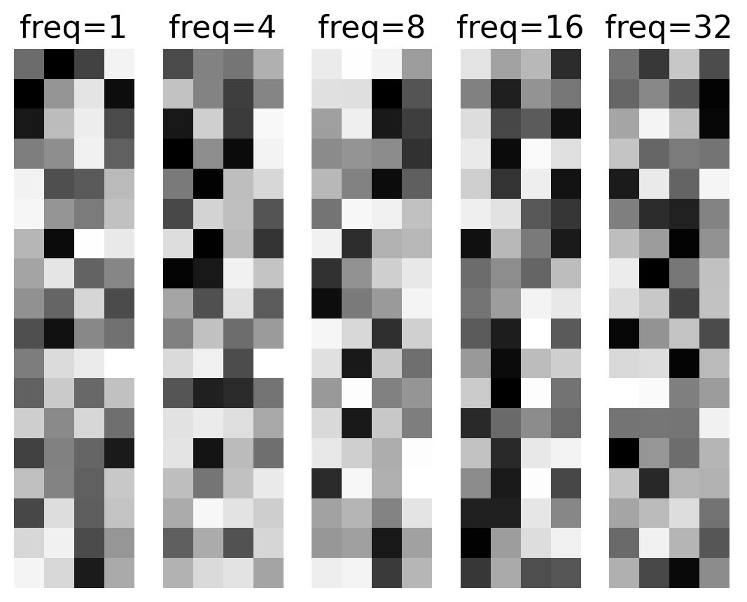
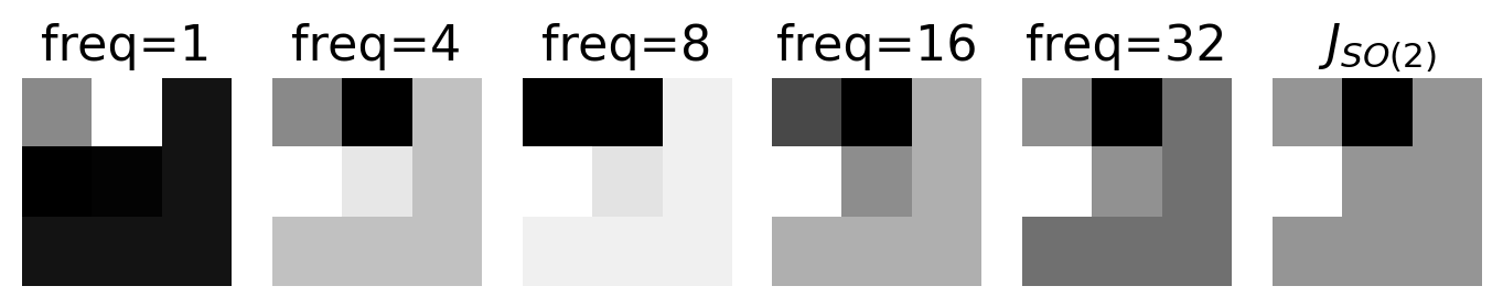
Figure 13: Left: the translation weight-sharing matrices and equivariance errors learned at different y-coordinates through MSR. Middle: learned rotation weight-sharing matrices by MSR at different frequencies of the channel flow. Right: learned SO(2) generators by LieGAN at different frequencies of the channel flow

Additionally, we conducted experiments with five distinct LieGAN models to capture the rotational symmetry in fluid dynamics across various scales. Initially, using the random initialization prescribed in the original study, LieGAN failed to identify any meaningful generators. Thus, we instead initialized the trainable generator as the true generator of SO(2) group and measured the symmetry breaking by checking how it deviates from the initialization after training. Figure 13 right visualizes the learned SO(2) generators by LieGAN at five different frequencies of the channel flow. The rightmost one is the true generator of SO2. It seems the generators learned on higher frequencies are closer to it than the ones learned on lower frequencies. However, a critical limitation of LieGAN is its inability to precisely measure the extent of symmetry breaking, unlike our proposed method.

Appendix F Distributional symmetry breaking with simple forward passing

Assume a probability distribution $p_{X}:X\to\mathbb{R}$ and a group $G$ that acts on $X$ by $\rho_{X}$. We have distributional symmetry breaking if $\forall x\in X$, $p_{X}(x)\neq p_{X}(\rho_{X}(g)x)$ (i.e the probability distribution does not remain closed under the group action). In this paper, we present the use of relaxed group convolution to uncover distributional symmetry breaking (i.e. for discovering homogeneity breaking in turbulence). However, we also present a complementary approach showing that group convolutions can detect distributional symmetry breaking on a single forward pass without training equivariant weights.

In a sequence of group convolutions, one usually averages over the group elements to return a function on $\mathbb{Z}^{3}$ (or the space of the desired input/output) after the last convolution. To instead detect symmetry breaking, one would not average over the group elements but would rather observe the pattern of the group elements after a single forward pass. Thus, given the output of a group convolution equivariant to a group $H$ as $f_{c}\in\mathbb{R}^{N\times c_{\text{out}}\times|H|\times\text{spatial dims}}$, we average over the spatial dimensions instead of $|H|$ after the last convolution. The network output will then be in $\mathbb{R}^{N\times c_{out}\times|H|}$.

We first illustrate this concept with a simple example. We consider a 3-layer $C_{4}$ equivariant randomly initialized group convolution network and show that the representation after a single forward pass (with no training) reflects the symmetry of the input seen in Figure 14. We observe that when the input is a square with $C_{4}$ symmetry the output averaged over spatial dimensions remain constant (up to any equivariance error of the model). For a rectangle with $C_{2}$ symmetry, the elements corresponding to $i$ and $g^{2}$ are the same while those corresponding to $g$ and $g^{3}$ are the same, thus also reflecting $C_{2}$ symmetry. For a shape with no symmetry, the output does not reflect symmetry across group elements.

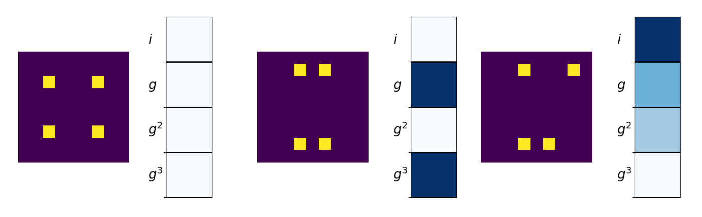
Figure 14: Visualization of input and corresponding output representatation after a single forward pass from a 3-layer $C_{4}$ equivariant group convolution network for 1) a square 2) a rectangle and 3) a non-symmetric object. These results are shown for a single random model initialization. When observing different model initializations, we found the same patterns for 1) and 2) and the lack of a pattern for 3).

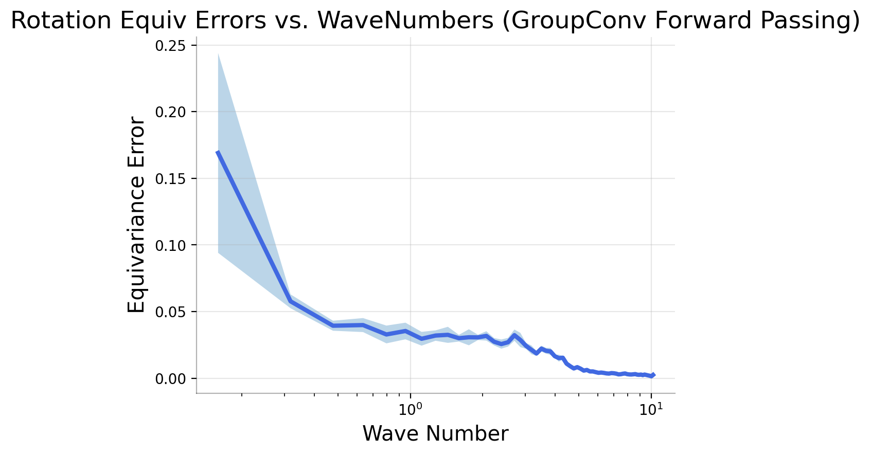
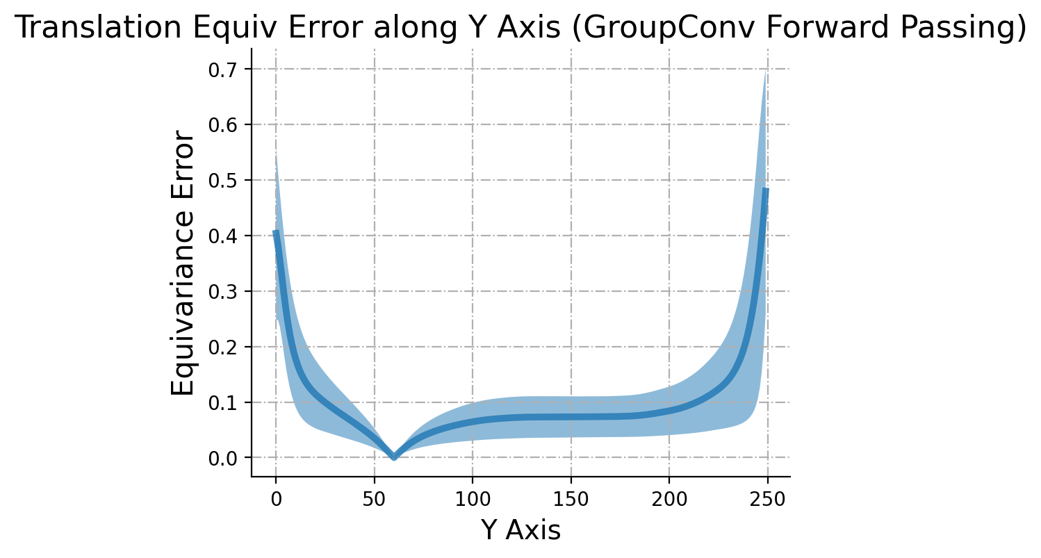
Figure 15: (Left) Rotational equivariance errors vs wavenumber and (right) translational equivariance errors along the y-axis for a single forward pass. The confidence intervals are calculated by 10 randomly initialized models.

We also explored this method for discovering isotropy breaking and homogeneity breaking in turbulence (Sections 5.2 and 5.3), as these are more complex examples of distributional symmetry breaking. As shown in 15, similar patterns to Figures 5 and 6 are recovered (up to rescaling of equivariance error). This demonstrates that this method could also be used for symmetry detection in the data distribution.

We emphasize that this method leverages the equivariant representations used in group convolutions to reflect the symmetry of a given input or data distribution. It is thus suitable when one wishes to detect broken symmetries, but could not be used to learn a mapping between input and output (e.g. in the case of functional symmetry breaking). For learning complex dynamics, relaxed group convolution is preferable, as it can automatically identify symmetry breaking and maintain the correct amount of equivariance, enabling end-to-end training with the right inductive bias.

Appendix G Additional Experiment with Relaxed Weights

To further explore the interpretability of relaxed weights, we performed an additional experiment using a 2-D smoke dataset generated with PhiFlow (Holl et al. (2020)). In PhiFlow, one can generate simulations with differential initial conditions and external forces from the incompressible Navier Stokes equations. We use a $C_{4}$ relaxed group convolution model and train it for forward prediction on a dataset with $C_{2}$ symmetry (2 simulations, one with a buoyancy force in the $+y$ direction and the other with a buoyancy force in the $-y$ direction). Each simulation has 300 timesteps. Steps 0-150 are used for training, 150-200 for validation, and 200-250 for testing. Forecasts are made in an autoregressive manner (using 6 input steps and 4 output steps) and are then evaluated on 10-step ahead prediction RMSEs, as in Wang et al. (2022). Note the model must be trained on these simulations together instead of separately to preserve $C_{2}$ symmetry.

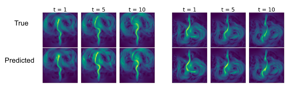
Figure 16: Velocity magnitude for target (ground truth) and model predictions at $t=1,5,10$ in the testing set for simulations in the $C_{2}$ symmetric dataset. The model seems to accurately capture the dynamics (test RMSE 0.645).

We then consider the learned relaxed weights for the model. As seen in Figure 17, they do exhibit $C_{2}$ symmetry, as the weights corresponding to the elements $i$ and $g^{2}$ are the same, as are the weights for the elements $g$ and $g^{3}$. We consider switching the relaxed weights with the corresponding $C_{2}$ group elements (i.e. swapping the $g$ and $g^{3}$ weights with the $i$ and $g^{2}$ weights). This is shown in Layer 3 in Figure 17.

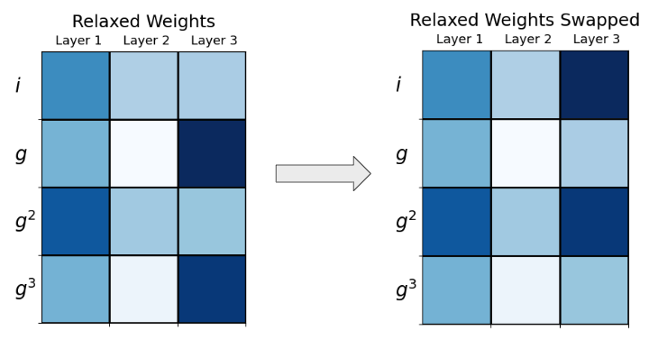
Figure 17: Learned relaxed weights for the $C_{4}$ model (right) and visualization of swapping the relaxed weights in the last layer.

As the original dataset contains buoyancy forces pointing up/down, we hypothesize that by swapping the relaxed weights of the trained model, we will be able to perform forward prediction on buoyancy forces pointing left/right with the trained model. To do so, we supply the model with an initial start from the testing set shown in Figure 18 rotated by 90 degrees. Forecasts are then made autoregressively for 50 timesteps.

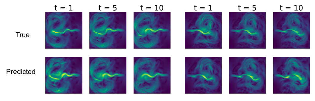
Figure 18: Velocity magnitude for target (ground truth) and model predictions at $t=1,5,10$ in the rotated testing set for simulations in the $C_{2}$ symmetric dataset. At earlier times $t<30$, the model performs somewhat comparably to the original model (test RMSE 0.79). However, at later times $30<t<50$, the performance degrades (test RMSE = 1.12) while still capturing notable features of the dataset (i.e. the main smoke plume).

By permuting the relaxed weights, we present a “proof of concept” forward prediction on rotated simulations reasonably well, demonstrating the interpretability of the relaxed weights. These predictions could potentially be improved by tuning model hyperparameters further or increasing the number of layers/relaxed group convolutions to more accurately capture the dynamics. In the future, we plan to further explore perturbing the relaxed weights for turbulence simulations.

References

- Dre (2008) Character of a Representation, pp. 29–55. Springer Berlin Heidelberg, Berlin, Heidelberg, 2008. doi: 10.1007/978-3-540-32899-5_3. URL https://doi.org/10.1007/978-3-540-32899-5_3.
- Anderson et al. (2019) Anderson, B., Hy, T.-S., and Kondor, R. Cormorant: Covariant molecular neural networks. In Advances in neural information processing systems (NeurIPS), 2019.
- Bao & Song (2019) Bao, E. and Song, L. Equivariant neural networks and equivarification. arXiv preprint arXiv:1906.07172, 2019.
- Batchelor (1953) Batchelor, G. K. The theory of homogeneous turbulence. Cambridge university press, 1953.
- Beekman et al. (2019) Beekman, A., Rademaker, L., and van Wezel, J. An introduction to spontaneous symmetry breaking. SciPost Physics Lecture Notes, pp. 011, 2019.
- Benidis et al. (2022) Benidis, K., Rangapuram, S. S., Flunkert, V., Wang, Y., Maddix, D., Turkmen, C., Gasthaus, J., Bohlke-Schneider, M., Salinas, D., Stella, L., et al. Deep learning for time series forecasting: Tutorial and literature survey. ACM Computing Surveys, 55(6):1–36, 2022.
- Bradley & Cracknell (2010) Bradley, C. and Cracknell, A. The mathematical theory of symmetry in solids: representation theory for point groups and space groups. Oxford University Press, 2010.
- Bronstein et al. (2021) Bronstein, M. M., Bruna, J., Cohen, T., and Veličković, P. Geometric deep learning: Grids, groups, graphs, geodesics, and gauges. arXiv:2104.13478, 2021.
- Castellani & Dardashti (2021) Castellani, E. and Dardashti, R. Symmetry breaking. In Knox, E. and Wilson, A. (eds.), The Routledge Companion to Philosophy of Physics. Routledge, 2021.
- Chidester et al. (2018) Chidester, B., Do, M. N., and Ma, J. Rotation equivariance and invariance in convolutional neural networks. arXiv preprint arXiv:1805.12301, 2018.
- Cohen & Welling (2016a) Cohen, T. and Welling, M. Group equivariant convolutional networks. In Proceedings of the International Conference on Machine Learning (ICML), 2016a.
- Cohen & Welling (2016b) Cohen, T. S. and Welling, M. Steerable CNNs. arXiv preprint arXiv:1612.08498, 2016b.
- Cohen et al. (2019) Cohen, T. S., Weiler, M., Kicanaoglu, B., and Welling, M. Gauge equivariant convolutional networks and the icosahedral CNN. In Proceedings of the 36th International Conference on Machine Learning (ICML), volume 97, pp. 1321–1330, 2019.
- Dehmamy et al. (2021) Dehmamy, N., Walters, R., Liu, Y., Wang, D., and Yu, R. Automatic symmetry discovery with lie algebra convolutional network. Advances in Neural Information Processing Systems, 34:2503–2515, 2021.
- Desai et al. (2022) Desai, K., Nachman, B., and Thaler, J. Symmetry discovery with deep learning. Physical Review D, 105(9):096031, 2022.
- Elsayed et al. (2020) Elsayed, G. F., Ramachandran, P., Shlens, J., and Kornblith, S. Revisiting spatial invariance with low-rank local connectivity. In Proceedings of the 37th International Conference of Machine Learning (ICML), 2020.
- Esteves et al. (2018) Esteves, C., Allen-Blanchette, C., Makadia, A., and Daniilidis, K. Learning so (3) equivariant representations with spherical cnns. In Proceedings of the European Conference on Computer Vision (ECCV), pp. 52–68, 2018.
- Fahle et al. (2001) Fahle, T., Schamberger, S., and Sellmann, M. Symmetry breaking. In Principles and Practice of Constraint Programming—CP 2001: 7th International Conference, CP 2001 Paphos, Cyprus, November 26–December 1, 2001 Proceedings 7, pp. 93–107. Springer, 2001.
- Finn et al. (2017) Finn, C., Abbeel, P., and Levine, S. Model-agnostic meta-learning for fast adaptation of deep networks. In International conference on machine learning, pp. 1126–1135. PMLR, 2017.
- Finzi et al. (2020) Finzi, M., Stanton, S., Izmailov, P., and Wilson, A. G. Generalizing convolutional neural networks for equivariance to lie groups on arbitrary continuous data. arXiv preprint arXiv:2002.12880, 2020.
- Finzi et al. (2021) Finzi, M. A., Benton, G., and Wilson, A. G. Residual pathway priors for soft equivariance constraints. In Beygelzimer, A., Dauphin, Y., Liang, P., and Vaughan, J. W. (eds.), Advances in Neural Information Processing Systems, 2021. URL https://openreview.net/forum?id=k505ekjMzww.
- Gao et al. (2023) Gao, H., Han, X., Fan, X., Sun, L., Liu, L.-P., Duan, L., and Wang, J.-X. Bayesian conditional diffusion models for versatile spatiotemporal turbulence generation. arXiv preprint arXiv:2311.07896, 2023.
- Geiger & Smidt (2022) Geiger, M. and Smidt, T. e3nn: Euclidean neural networks. arXiv preprint arXiv:2207.09453, 2022.
- Ghosh & Gupta (2019) Ghosh, R. and Gupta, A. K. Scale steerable filters for locally scale-invariant convolutional neural networks. arXiv preprint arXiv:1906.03861, 2019.
- Helwig et al. (2023) Helwig, J., Zhang, X., Fu, C., Kurtin, J., Wojtowytsch, S., and Ji, S. Group equivariant fourier neural operators for partial differential equations. arXiv preprint arXiv:2306.05697, 2023.
- Holl et al. (2020) Holl, P. M., Um, K., and Thuerey, N. phiflow: A differentiable pde solving framework for deep learning via physical simulations. In Workshop on Differentiable Vision, Graphics, and Physics in Machine Learning at NeurIPS, 2020.
- Jain et al. (2013) Jain, A., Ong, S. P., Hautier, G., Chen, W., Richards, W. D., Dacek, S., Cholia, S., Gunter, D., Skinner, D., Ceder, G., et al. Commentary: The materials project: A materials genome approach to accelerating materials innovation. APL materials, 1(1), 2013.
- Jucha et al. (2014) Jucha, J., Xu, H., Pumir, A., and Bodenschatz, E. Time-reversal-symmetry breaking in turbulence. Physical review letters, 113(5):054501, 2014.
- Kanov et al. (2015) Kanov, K., Burns, R., Lalescu, C., and Eyink, G. The johns hopkins turbulence databases: An open simulation laboratory for turbulence research. Computing in Science & Engineering, 17(5):10–17, 2015.
- Knigge et al. (2022) Knigge, D. M., Romero, D. W., and Bekkers, E. J. Exploiting redundancy: Separable group convolutional networks on lie groups. In International Conference on Machine Learning, pp. 11359–11386. PMLR, 2022.
- Kondor & Trivedi (2018) Kondor, R. and Trivedi, S. On the generalization of equivariance and convolution in neural networks to the action of compact groups. In Proceedings of the 35th International Conference on Machine Learning (ICML), volume 80, pp. 2747–2755, 2018.
- Lamb & Roberts (1998) Lamb, J. S. and Roberts, J. A. Time-reversal symmetry in dynamical systems: a survey. Physica D: Nonlinear Phenomena, 112(1-2):1–39, 1998.
- Landau (1936) Landau, L. The theory of phase transitions. Nature, 138(3498):840–841, 1936.
- Liao et al. (2023) Liao, Y.-L., Wood, B., Das, A., and Smidt, T. Equiformerv2: Improved equivariant transformer for scaling to higher-degree representations. arXiv preprint arXiv:2306.12059, 2023.
- Liu et al. (2022) Liu, Y., Wang, L., Liu, M., Lin, Y., Zhang, X., Oztekin, B., and Ji, S. Spherical message passing for 3d molecular graphs. In International Conference on Learning Representations, 2022. URL https://openreview.net/forum?id=givsRXsOt9r.
- Luke et al. (1998) Luke, G. M., Fudamoto, Y., Kojima, K., Larkin, M., Merrin, J., Nachumi, B., Uemura, Y., Maeno, Y., Mao, Z., Mori, Y., et al. Time-reversal symmetry-breaking superconductivity in sr2ruo4. Nature, 394(6693):558–561, 1998.
- McNeela (2023) McNeela, D. Almost equivariance via lie algebra convolutions. arXiv preprint arXiv:2310.13164, 2023.
- Nabarro (1947) Nabarro, F. Dislocations in a simple cubic lattice. Proceedings of the Physical Society, 59(2):256, 1947.
- Onuki (2002) Onuki, A. Phase transition dynamics. Cambridge University Press, 2002.
- Otto et al. (2023) Otto, S. E., Zolman, N., Kutz, J. N., and Brunton, S. L. A unified framework to enforce, discover, and promote symmetry in machine learning. arXiv preprint arXiv:2311.00212, 2023.
- Passaro & Zitnick (2023) Passaro, S. and Zitnick, C. L. Reducing so (3) convolutions to so (2) for efficient equivariant gnns. arXiv preprint arXiv:2302.03655, 2023.
- Petrache & Trivedi (2023) Petrache, M. and Trivedi, S. Approximation-generalization trade-offs under (approximate) group equivariance. arXiv preprint arXiv:2305.17592, 2023.
- Pope (2001) Pope, S. B. Turbulent flows. Measurement Science and Technology, 12(11):2020–2021, 2001.
- Satorras et al. (2021a) Satorras, V. G., Hoogeboom, E., and Welling, M. E(n) equivariant graph neural networks. arXiv preprint arXiv:2102.09844, 2021a.
- Satorras et al. (2021b) Satorras, V. G., Hoogeboom, E., and Welling, M. E (n) equivariant graph neural networks. In International Conference on Machine Learning, pp. 9323–9332. PMLR, 2021b.
- Schütt et al. (2017) Schütt, K., Kindermans, P.-J., Sauceda Felix, H. E., Chmiela, S., Tkatchenko, A., and Müller, K.-R. Schnet: A continuous-filter convolutional neural network for modeling quantum interactions. Advances in neural information processing systems, 30, 2017.
- Smidt et al. (2021) Smidt, T. E., Geiger, M., and Miller, B. K. Finding symmetry breaking order parameters with euclidean neural networks. Physical Review Research, 3(1):L012002, 2021.
- Strocchi (2005) Strocchi, F. Symmetry breaking, volume 643. Springer, 2005.
- Thomas et al. (2018) Thomas, N., Smidt, T., Kearnes, S., Yang, L., Li, L., Kohlhoff, K., and Riley, P. Tensor field networks: Rotation-and translation-equivariant neural networks for 3d point clouds. arXiv preprint arXiv:1802.08219, 2018.
- Van der Laan & Kirkman (1992) Van der Laan, G. and Kirkman, I. The 2p absorption spectra of 3d transition metal compounds in tetrahedral and octahedral symmetry. Journal of Physics: Condensed Matter, 4(16):4189, 1992.
- van der Ouderaa et al. (2023) van der Ouderaa, T. F., Immer, A., and van der Wilk, M. Learning layer-wise equivariances automatically using gradients. arXiv preprint arXiv:2310.06131, 2023.
- Walters et al. (2021) Walters, R., Li, J., and Yu, R. Trajectory prediction using equivariant continuous convolution. International Conference on Learning Representations, 2021.
- Wang et al. (2020) Wang, R., Walters, R., and Yu, R. Incorporating symmetry into deep dynamics models for improved generalization. In International Conference on Learning Representations (ICLR), 2020.
- Wang et al. (2022) Wang, R., Walters, R., and Yu, R. Approximately equivariant networks for imperfectly symmetric dynamics. In International Conference on Machine Learning, pp. 23078–23091. PMLR, 2022.
- Weiler & Cesa (2019) Weiler, M. and Cesa, G. General E(2)-equivariant steerable CNNs. In Advances in Neural Information Processing Systems (NeurIPS), pp. 14334–14345, 2019.
- Weinberg (1976) Weinberg, S. Implications of dynamical symmetry breaking. Physical Review D, 13(4):974, 1976.
- Woodward (1997) Woodward, P. M. Octahedral tilting in perovskites. i. geometrical considerations. Acta Crystallographica Section B: Structural Science, 53(1):32–43, 1997.
- Worrall et al. (2017) Worrall, D. E., Garbin, S. J., Turmukhambetov, D., and Brostow, G. J. Harmonic networks: Deep translation and rotation equivariance. In Proceedings of the IEEE Conference on Computer Vision and Pattern Recognition, pp. 5028–5037, 2017.
- Yang et al. (2023a) Yang, J., Dehmamy, N., Walters, R., and Yu, R. Latent space symmetry discovery. arXiv preprint arXiv:2310.00105, 2023a.
- Yang et al. (2023b) Yang, J., Walters, R., Dehmamy, N., and Yu, R. Generative adversarial symmetry discovery. arXiv preprint arXiv:2302.00236, 2023b.
- Ying et al. (2018) Ying, B., Yuan, K., Vlaski, S., and Sayed, A. H. Stochastic learning under random reshuffling with constant step-sizes. IEEE Transactions on Signal Processing, 67(2):474–489, 2018.
- Zaheer et al. (2017) Zaheer, M., Kottur, S., Ravanbakhsh, S., Poczos, B., Salakhutdinov, R., and Smola, A. Deep sets. arXiv preprint arXiv:1703.06114, 2017.
- Zakharov et al. (2012) Zakharov, V. E., L’vov, V. S., and Falkovich, G. Kolmogorov spectra of turbulence I: Wave turbulence. Springer Science & Business Media, 2012.
- Zhang (1988) Zhang, W. Shift-invariant pattern recognition neural network and its optical architecture. In Proceedings of annual conference of the Japan Society of Applied Physics, 1988.
- Zhou et al. (2021) Zhou, A., Knowles, T., and Finn, C. Meta-learning symmetries by reparameterization. In International Conference on Learning Representations, 2021. URL https://openreview.net/forum?id=-QxT4mJdijq.
- Zitnick et al. (2022) Zitnick, L., Das, A., Kolluru, A., Lan, J., Shuaibi, M., Sriram, A., Ulissi, Z., and Wood, B. Spherical channels for modeling atomic interactions. Advances in Neural Information Processing Systems, 35:8054–8067, 2022.