CLIP Is Also a Good Teacher: A New Learning Framework for Inductive Zero-shot Semantic Segmentation

Abstract

Existing Generalized Zero-shot Semantic Segmentation (GZLSS) methods apply either finetuning the CLIP paradigm or formulating it as a mask classification task, benefiting from the Vision-Language Models (VLMs). However, the fine-tuning methods are restricted with fixed backbone models which are not flexible for segmentation, and mask classification methods heavily rely on additional explicit mask proposers. Meanwhile, prevalent methods utilize only seen categories which is a great waste, i.e., neglecting the area exists but not annotated. To this end, we propose CLIPTeacher, a new learning framework that can be applied to various per-pixel classification segmentation models without introducing any explicit mask proposer or changing the structure of CLIP, and utilize both seen and ignoring areas. Specifically, CLIPTeacher consists of two key modules: Global Learning Module (GLM) and Pixel Learning Module (PLM). Specifically, GLM aligns the dense features from an image encoder with the CLS token, i.e., the only token trained in CLIP, which is a simple but effective way to probe global information from the CLIP models. In contrast, PLM only leverages dense tokens from CLIP to produce high-level pseudo annotations for ignoring areas without introducing any extra mask proposer. Meanwhile, PLM can fully take advantage of the whole image based on the pseudo annotations. Experimental results on three benchmark datasets: PASCAL VOC 2012, COCO-Stuff 164k, and PASCAL Context show large performance gains, i.e., 2.2%, 1.3%, and 8.8%.

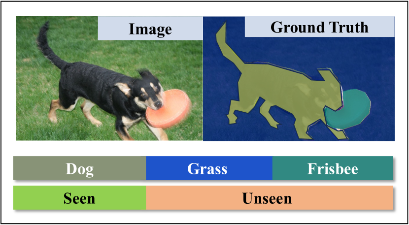
(a) an image and its annotation

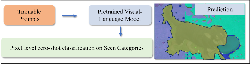
(b) Finetuning based methods, e.g., zegclip [55]

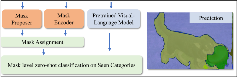
(c) Mask proposer based methods, e.g., zegformer [16]

(d) Our methods

Figure 1: Existing VLM-based GZLSS methods apply either (a): finetuning-based methods or (b) mask proposer-based methods. Both of these methods suffer from the inflexibility of model structures and the insufficient utilization of ignoring areas.

1 Introduction

Semantic segmentation, as one of the most significant tasks in computer vision, has made remarkable progress in recent years benefiting from the rapid development of deep learning technology [26, 42, 44]. For modern semantic segmentation models, a large amount of high-quality data is required to achieve state-of-the-art performance. However, collecting such data is very expensive and time-consuming, e.g., each image in the Cityscapes [14] dataset takes 1.5 hours accounting for quality control. With the development of large-scale Vision-Language Models (VLMs), represented by CLIP [40], ALIGN [28] and RAM [52], pure vision models, for the first time, are aligned with the natural language and are capable to do zero-shot vision tasks, e.g. zero-shot semantic segmentation, which releases the training of vision models from a huge amount of manually annotated data.

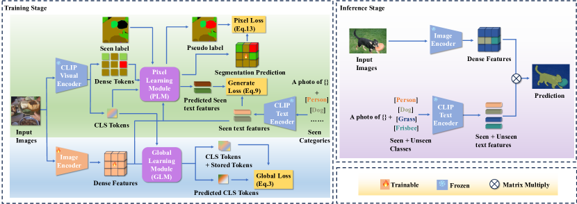
Figure 2: The overall structure of CLIPTeacher. The black area in the ”Seen label” is the unannotated area (unseen categories), and the areas with other color is the annotated area (seen categories).

Though remarkable, these models are trained by aligning the information between a whole image and its corresponding text pairs, which suggests VLMs lack the ability to localize and classify multiple objects in one image and are not suitable for segmentation tasks. To mitigate this issue, some early works [30, 19] try to directly fine-tune the pretrained VLMs, however, as the lack of data and proper fine-tuning methods, the performance is compromised. Recently, inspired by the Visual Prompt Tuning (VPT) [29] and the appearance of the adapter structure [27], as shown in Fig. 1, some works [55, 50, 54, 21] that utilize these two strategies simultaneously or respectively to efficiently finetune the VLMs also attracted much attention from the research endeavors. Another solution shown in Fig. 1 is based on the pretrained [51, 41] or online learning mask proposer [39, 17, 16] to find and learns from all the objects including seen and potential ones. Despite the pioneer researchers’ huge steps, prevalent works still have some drawbacks. 1) These works above are still stuck in the specified structures, i.e., the backbone can be only selected from ViT [18] or ResNet [26] for finetuning-based methods, and for the mask proposer-based methods an explicit mask proposer whose quality highly affects the performance is required during training. 2) Both learning frameworks can only utilize the seen categories during training, which leads to compromising performance.

To address the challenges above, we propose a simple but effective training framework called CLIPTeacher as shown in Fig. 2. CLIPTeacher helps any semantic segmentation model including those designed for closed-set, e.g., ConvNext [33], Segformer [49], to do zero-shot semantic segmentation without adding any change to the existing CLIP model. Furthermore, CLIPTeacher can fully utilize both seen and ignored areas, i.e., the regions that exist but are not annotated, which avoids the great waste of images. Specifically, except for the CLIP and the segmentation models, we propose two new modules in the CLIPTeacher: a global learning module (GLM), and a pixel learning module (PLM). In GLM, since only the CLS token is trained in CLIP, we apply a self-attention-based structure to align the CLS token from the pretained VLMs and the dense features from the segmentation model. In PLM, inspired by PACL [35] and DINO [4] that indicate the dense tokens output by CLIP are highly semantically coherent, i.e., the output tokens belonging to semantically similar regions in an image are similar with each other, we propose a multi-scale K-Means algorithm along with a mask fusion algorithm to find the potential objects from the area without any annotation in an image. The potential objects along with the seen labels are fused serving as the pseudo labels for the segmentation models. Though the pseudo labels are generated, the classifiers for those potential objects are still missing. As a result, we approach a transformer-decoder-based Vision-Language Adapter (VLA) to produce the weights for the generated potential objects. We conducted extensive experiments on three benchmark datasets on Zero-shot semantic segmentation: PASCAL VOC 2012, COCO-Stuff 164k, and PASCAL Context datasets. Compared with SOTA, our method outperforms 5 points, 5 points, and 12 points on these three benchmarks, respectively.

2 Related Works

2.1 Closed-set Semantic Segmentation

Prevalent semantic segmentation can be grouped into two aspects: pixel-level classification and mask-level classification. For pixel-level classification, FCN [34] as the first fully convolutional network to employ end-to-end semantic segmentation introduces 1 $\times$ 1 as the decode head, which determines the paradigm of pixel-level semantic segmentation. Since FCN, many works, e.g., DeepLab series [6, 5], Deformable convolution [15], aim to enlarge the receptive field to further improve the performance of pixel-level methods. With the appearance of self-attention [44] and ViT [18], many works [53, 49, 22, 32] replace the conventional convolutional backbone to the self-attention-based one and achieved remarkable performance. Another aspect treats the semantic segmentation tasks as a mask classification task. MaskFormer [11] and Mask2Former [10] are two representative works. Specifically, these models first generate several object queries containing positional information. Then these object queries are converted into masks through a mask proposer. Finally, object queries and masks are applied to do classification and mask prediction tasks, respectively.

However, these methods have some drawbacks. Specifically, they are designed for closed datasets, which limits their ability to discriminate between a limited number of categories in the training dataset. Additionally, achieving state-of-the-art performance requires a large amount of annotated high-quality images, which are expensive and time-consuming to collect for training a segmentation model. In contrast, our proposed CLIPTeacher can be applied to any per-pixel segmentation model to enable zero-shot semantic segmentation. It frees the per-pixel semantic segmentation model from the limitations of a specified dataset and the need for high-quality data that is expensive and time-consuming to collect.

2.2 Zero-shot Semantic Segmentation

Before the large-scale VLMs, e.g., CLIP [40], several works [20, 47] try to bridge the gap between vision and language by mapping the dense features extracted from the vision models to the text features extracted from the language models. However, due to the sparsity of image-text pairs, these models did not get competitive results. With the appearance of large-scale VLMs, represented by CLIP [40] and ALIGN [28], zero-shot vision tasks have entered a new era. For zero-shot semantic segmentation tasks, there are two popular solutions: Fintuning VLMs and introducing an explicit mask proposer. For the first solution [50, 30, 19, 55, 54, 21], benefiting from visual prompt tuning [29] and adapter [27], this method introduces some trainable parameters for the VLMs which are only trained in image level and an adapter to further help the dense tokens obtain the pixel-level segmentation ability. Unfortunately, this method sacrifices the flexibility of the segmentation model, i.e., the backbone of the segmentation model has to be ResNet or ViT. For the second solution [39, 51, 41, 17, 16], this method benefiting from the success of mask-level semantic segmentation [10, 11] decouples the semantic segmentation into category loss and class-agnostic mask loss. However, this type of method has to introduce extra parameters and the quality of proposed masks is highly related to the performance of the segmentation model.

Motivated by recent advances in understanding the CLIP model [35] and unsupervised learning [23], we propose a novel training structure for any pixel-level semantic segmentation models without introducing any explicit mask proposer. Meanwhile, we can also take advantage of the ignoring areas that exist but are not annotated. The most related works are MaskCLIP [54] and ZS3/ZS5 [3]. Different from MaskCLIP, our methods do not change any structure of CLIP rather than replacing the self-attention to the 1 $\times$ 1 convolution layer, and our methods are applied to inductive rather than transductive settings. For ZS3/ZS5, their training includes two individual steps, however, our methods do not need any additional training steps.

3 Methods

3.1 Preliminary and Method Overview

Inductive GZLSS. Our proposed methods follow the inductive settings that have been widely applied in generalized zero-shot semantic segmentation (GZLSS) [48, 55, 16, 3]. For inductive settings, before the training stage, the categories in a training dataset are separated into two groups: seen categories $\mathcal{S}^{s}$ and unseen categories $\mathcal{S}^{u}$. Note that there is no overlap between the two groups $\mathcal{S}^{u}\cap\mathcal{S}^{s}=\varnothing$. In the training stage, only the pixel-level annotations of $\mathcal{S}^{s}$ can be accessed and the existence of $\mathcal{S}^{s}$ is known. The annotations belonging to the unseen categories are replaced by the same ”ignored area” and do not contribute to the loss. While in the inference stage, both the $\mathcal{S}^{u}$ and $\mathcal{S}^{s}$ need to be segmented properly.

The greatest challenge that the remarkable semantic segmentation models can not be applied in the GZLSS is the lack of the semantic discriminative pixel-level annotations for the ”ignored area” leading to severe overfitting to the seen categories. In this paper, our method effectively utilizes the ”ignore area” and enables the remarkable semantic segmentation models to be applied in the GZLSS.

Method overview. We aim to make any pixel-level semantic segmentation networks fit for the GZLSS. However, due to the lack of pixel-level supervision for the unseen categories, only learning from the seen categories leads to severe overfitting to the seen categories. As a result, a method that discovers and discriminates between the seen and the potential categories needs to be proposed. Consequently, we approach two novel modules termed Global Learning Module (GLM) and Pixel Learning Module (PLM), as shown in Figure 2. The GLM is proposed to learn from the CLS token in the CLIP visual encoder that contains the global information including both seen and potential categories of an input image. GLM can help the image encoder produce a better representation that aligns with the text features, especially for the unseen categories. Inspired by the research that the tokens generated by the transformer are highly semantically correlated [35, 4, 23], PLM can first find the potential categories by simply clustering on the dense tokens from the CLIP visual encoder. Meanwhile, based on the generated pseudo label, PLM also produces pseudo weights to further distinguish between different potential categories as well as the seen categories.

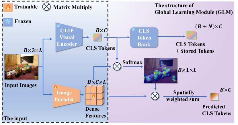
Figure 3: The structure of Global Learning Module (GLM).

3.2 Global Learning Module

CLIP [40] with the backbone of ViT [18], as one of the most famous Vision-Language models, is trained by aligning the features between the whole images and their corresponding text pairs, which indicates that only the CLS token plays the role of bridging the gap between vision and text. Therefore, to fully take advantage of the CLS token, we carefully design the Global Learning Module (GLM) inspired by the self-attention structure [44, 45]. The structure of GLM is depicted in Figure 3.

The core design of GLM is a self-attention-based weighted sum among the dense features output by the segmentation model. Specifically, an input image is fed into a trainable segmentation model and a frozen CLIP visual encoder to obtain the dense features $\mathcal{R}^{B*C*L}$ and the CLS token $\mathcal{S}^{B*C}$ where $B$ indicates the batch number, $C$ is the channel number of output representations and $L=H*W$ is the multiplication of the height and width of dense features. Different from all the existing self-attention-based methods [44, 45, 18], we do not introduce any trainable parameters to produce Q, K, and V. The CLS tokens act as the Q directly and dense features as K and V. The weight $W$ is generated by the inner product of $\mathcal{S}$ and $\mathcal{R}$:

$$W=\text{Softmax}\frac{\mathcal{S}\cdot\mathcal{R}}{\sqrt{C}},$$ (1)

where $W^{B\times L}\in[0,1]$. The weight $w_{i}\in W$ for the $i$th feature $r_{i}\in\mathcal{R}$ is the softmax along the $\mathcal{L}$. Once the weight is generated, we apply the inner product to the $W$ and the $\mathcal{R}$ to produce the predicted CLS token $\hat{\mathcal{S}}$:

$$\hat{\mathcal{S}}=W\cdot\mathcal{R}^{T}.$$ (2)

Motivated by the success of contrastive learning [25, 9, 7, 8], we apply the InfoNCE [36] as the loss function to do contrastive learning between $s_{i}\in\mathcal{S}$ and $\hat{s}_{i}\in\hat{\mathcal{S}}$. To better learn the information embedded in the CLS token, inspired by the success of memory bank [25, 46], we propose a CLS token bank to store the previous CLS tokens. Let $\mathcal{V}_{n}=\left\{\mathcal{S}_{t-1},\mathcal{S}_{t-2}......\mathcal{S}_{t-n}\right\}$ be the CLS token bank where $t$ indicates the number of iterations, and $n$ indicates the size of the CLS token bank. During training, before the parameter update, we pop out the $\mathcal{S}_{t-n}$ in $\mathcal{V}$ and insert the $\mathcal{S}_{t}$ to $\mathcal{V}$. To be specific, the loss for the GLM is,

$$\mathcal{L}_{global}=\Sigma_{i}^{B}{\frac{\exp(s^{T}_{i}\cdot\hat{s}_{i}/\tau)}{\Sigma_{j\neq i}^{B*n}{\exp(s_{j}^{T}\cdot\hat{s}_{i})/\tau})+\exp(s^{T}_{i}\cdot\hat{s}_{i}/\tau)}},$$ (3)

where $B$ describes the batch number, $\tau$ indicates the temperature for the contrastive loss.

We think the GLM can work because all the dense features are aligned with the CLS token, which is the only token trained in CLIP. Consequently, the dense features are aligned with the text features of the CLIP text encoder, i.e., the classifier for the segmentation. Besides, the alignment between the dense features and the CLS tokens helps the segmenter learn from the ignoring areas when there is a potential object. In addition, the most representative regions can also be found, which is beneficial for learning a better representation. More results are shown in Section 4.4.

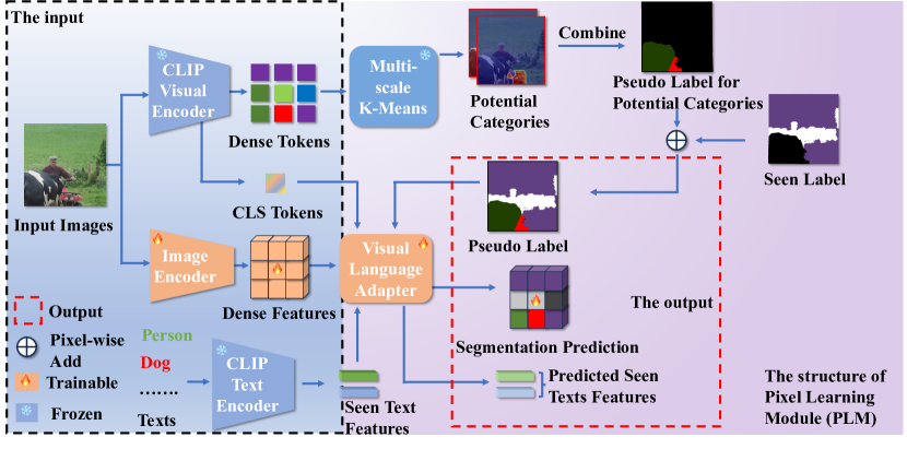
(a) The overview of Pixel Learning Module (PLA).

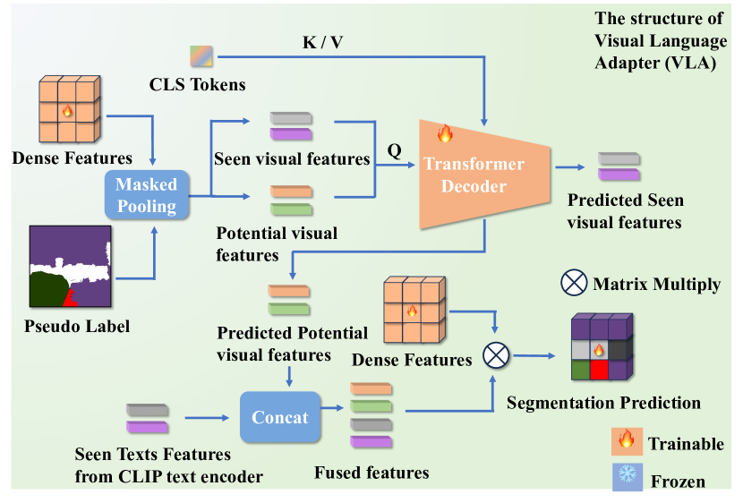
(b) The structure of Visual Language Adapter (VLA).

Figure 4: The structure of Pixel Learning Module. The white color indicates the seen categories, and the black area implies the potential areas including both unseen and ignored areas.

3.3 Pixel Learning Module

The general practice of semantic segmentation is treated as a pixel-level classification task. As a result, relying only on the GLM can not handle the fine-grained semantic segmentation problem. Meanwhile, for GZLSS, we can not explicitly learn from the ignoring areas, failing to learn the information of ignoring areas. To mitigate these issues, we propose a Pixel Learning Module (PLM). The structure of PLM is shown in Fig. 4. PLM consists of a multi-scale K-means clustering algorithm to find the potential objects serving as the pseudo labels for ignoring areas and a Visual-Language Adapter (VLA) to generate pseudo weights for pixel-level supervision. We will introduce each of the components in the following.

Multi-scale K-means clustering. One of the greatest challenges for GLZSS is the lack of unseen category annotations, which prevents the segmentation model from learning pixel-level information about the ignoring areas. Consequently, we revisit the purpose of the mask proposer and argue that only semantically similar regions are required to produce the pixel-level annotations for the potential objects. Previous research endeavors have found that the features of the models trained by the self-supervised [4, 37] and unsupervised [23] framework are highly correlated. For the CLIP model, this property has also been studied [35]. Motivated by these works, we propose Multi-scale K-means clustering to discover the semantically similar regions for the pixel-level pseudo labels. Specifically, we feed the same input images as the image encoder into the fixed CLIP visual encoder and obtain the output dense tokens. Then inspired by the SLIC algorithm [1], we initialize several centers with different sizes of windows on the dense tokens,

$$K_{h}=\frac{H}{s},K_{w}=\frac{W}{s},$$ (4)

$$C_{d}=\sum_{s}^{S}\sum_{i=0}^{K_{w}}\sum_{j=0}^{K_{h}}{\frac{D(i+s,j+s)}{K_{w}\cdot K_{h}}},$$ (5)

where $K_{h}$, $K_{w}$ implies the strides of the window along the height and the width, $H$, $W$ indicates the height and the width of the dense tokens, $S$ indicates the sizes of windows, and $D$ indicates the output dense tokens. Once the centers $C_{d}$ are initialized, we apply K-Means clustering based on these centers only on ignored areas, i.e., without any annotations, to produce the pseudo labels for ignoring areas. However, as a large number of centers, only relying on K-Means leads to too small and many regions. Therefore, we propose a mask fusion algorithm inspired by NMS [31, 43] widely applied in object detection to remove the redundant bounding boxes shown in the Algorithm. 1.

Algorithm 1

1:  Initialize the threshold $\lambda$, and the masks $\mathcal{M}^{N*H*W}\in{0,1}$ generated by $C_{d}$ # Initialize the masks to be fused and the threshold for fusion.

2:  Initialize $F=\varnothing$ # Initialize the fusion centers.

3:  $\mathcal{S}=\frac{T\cdot T^{T}}{|T|^{2}}$, # Compute the cosine similarity among all the centers.

4:  $c_{max}=\max(\mathcal{S})$

5:  while $c_{max}>=\lambda$ do

6:     $index=where(c_{max})[0]$ # Find the row where the max value is.

7:     $mask=\mathcal{S}[index]>\lambda$

8:     $F$.append($\mathcal{M}$[mask].sum(0))# Add the temporal results to the list of $\beta$.

9:     $\mathcal{S}$[index,:] = -100# The masks selected can not be selected again..

10:     $\mathcal{S}$[:,index] = -100# The masks selected can not be selected again..

11:     $c_{max}=\max(\mathcal{S})$

12:  end while

13:  return  $F$

Visual-Language Adapter. Another challenge for pixel-level learning in GZLSS is the lack of a classifier for unseen areas. To address this issue, we propose a visual language adapter (VLA) as shown in Fig. 4. Note that the VLA is only applied during training. Specifically, we obtain the seen and the potential visual features based on the $F$ generated by the Algorithm. 1, and obtain the corresponding centroid by averaging the corresponding area,

$$L_{a}=cat(L_{seen},F),$$ (6)

$$p_{l}=\frac{\sum_{B,H,W}{\mathcal{R}[\mathbb{1}(y=l_{a})]}}{\sum_{B,H,W}[\mathbb{1}(y=l_{a})]},$$ (7)

where $B$ represents the batch size of the input images. $H$, $W$ respectively indicate the height and width of the input images. $\mathcal{R}$ implies the dense features output by the segmentation models, $cat$ depicts the concatenation operation, and $l_{a}\in L_{a}$ indicates the segmentation label including both seen and ignoring areas found by multi-scale K-Means. Then the seen and the potential features are fed into a transformer decoder as query and the CLS tokens from the CLIP visual encoder as key and value. The generated features are divided into two parts: generated seen features and generated potential features. As for inductive settings, the information for unseen categories is not accessed, to guarantee the quality of the generated potential features, We apply an MSE loss between the generated seen features and their corresponding text features from the CLIP text encoder:

$$\mathcal{L}_{generate}=\Sigma_{i=0}^{s_{seen}}||p_{i}-t_{i}||^{2},$$ (8)

where $p_{i}\in P$ represents the generated seen features corresponding to the $i$th seen category, and $t_{i}\in T$ is the $i$th corresponding text features from the CLIP text encoder.

The generated unseen features are yielded as the classifier to be distinguished between both seen categories and different ignoring areas,

$$x=\mathcal{R}^{T}\cdot cat(P_{u},T),$$ (9)

$$\mathcal{L}_{ce}=CE(x,L_{all}),$$ (10)

where $P_{u}\in P_{all}$ indicates the potential features produced by the generator, $T$ indicates the text features produced by the CLIP text encoder with the name of seen categories, and $CE$ indicates the cross entropy loss.

3.4 Training Objective and Inference

Training Objective. The total loss functions are the combination of the global loss for GLM and the pixel loss for PLM:

$$\mathcal{L}_{inductive}=\mathcal{L}_{global}+\mathcal{L}_{pixel}+\mathcal{L}_{generate},$$ (11)

$$\mathcal{L}_{pixel}=\mathcal{L}_{CE}+\mathcal{L}_{focal}+\mathcal{L}_{dice},$$ (12)

where $\mathcal{L}_{focal}$ and $\mathcal{L}_{dice}$ are the same as the NEL in applied in ZegCLIP [55].

Inference. We follow the normal inference procedure as most of the segmentation works [34, 5, 49] that only use the features from the image encoder, and the logits are produced by the inner product between the text features from the CLIP text encoder and the image encoder features. As the lack of unseen categories, though our method can distinguish between different categories, we add a specified value $\gamma$ to the logits of unseen categories.

Table 1: Comparison with state-of-the-art methods where the bold and the underline indicates the best and the second-best performance.

Models	Publication	PASCAL VOC 2012				COCO-Stuff 164K				PASCAL Context
		pAcc	mIoU(S)	mIoU(U)	hIoU	pAcc	mIoU(S)	mIoU(U)	hIoU	pAcc	mIoU(S)	mIoU(U)	hIoU
SPNet [47]	CVPR19	-	78.0	15.6	26.1	-	35.2	8.7	14.0	-	-	-	-
ZS3 [3]	NIPS19	-	77.3	17.7	28.7	-	34.7	9.5	15.0	52.8	20.8	12.7	15.8
CaGNet [20]	MM20	80.7	78.4	26.6	39.7	56.6	33.5	12.2	18.2	-	24.1	18.5	21.2
SIGN [12]	ICCV21	-	75.4	28.9	41.7	-	32.3	15.5	20.9	-	-	-	-
Joint [2]	ICCV21	-	77.7	32.5	45.9	-	-	-	-	-	33.0	14.9	20.5
ZegFormer [16]	CVPR22	-	86.4	63.6	73.3	-	36.6	33.2	34.8	-	-	-	-
zzseg [51]	ECCV22	90.0	83.5	72.5	77.5	60.3	39.3	36.3	37.8	-	-	-	-
ZegCLIP [55]	CVPR23	94.6	91.9	77.8	84.3	62.0	40.2	41.4	40.8	76.2	46.0	54.6	49.9
DeOP [24]	ICCV23	-	88.2	74.6	80.8	-	38.0	38.4	38.2	-	-	-	-
SegNext+ours [22]	NIPS22	94.0	89.2	82.2	85.6	62.8	42.8	39.3	41.0	80.4	51.8	56.1	53.7
Swin-B+ours [32]	ICCV21	93.7	88.4	81.9	85.1	62.3	43.8	37.7	40.5	81.6	53.5	65.0	58.7
Segformer-B4+ours [49]	NIPS21	93.3	89.6	83.6	86.5	63.5	43.3	41.0	42.1	81.7	53.0	64.9	58.4

4 Experiments

4.1 Dataset

To evaluate the effectiveness of our methods, we select three representative benchmarks: PASCAL VOC, COCO-Stuff 164k, and PASCAL Context to conduct our experiments. The split of seen and unseen categories follows the setting of the previous works [16, 55, 51, 54]. We introduce the details of these three datasets.

PASCAL VOC consists of 10582 images for training and 1449 images for validation. Note that we convert the ’background’ category to the ’ignore’ category in both inductive and transductive settings. For this dataset, there are 15 seen categories and 5 unseen categories.

COCO-Stuff 164k contains 171 categories totally. As in previous settings, 171 categories are split into 156 seen and 15 unseen categories. Besides, for the training dataset, there are 118287 images and 5000 images for testing.

PASCAL Context includes 4996 images for training and 5104 images for testing. For the zero-shot semantic segmentation task, the dataset is split into 49 seen categories and 10 unseen categories.

4.2 Implementation Details

The proposed methods are implemented on the open-source toolbox MMsegmentation [13] with Pytorch 2.0.1 [38]. The CLIP model applied in our method is based on the ViT-B/16 model and the channel ($C$) of the output text features is 512. All the experiments are conducted on 8 V100 GPUs and the batch size ($B$) is set to 16 for all three datasets. For all these three datasets, the size of the input images is set as 512 ($H$) $\times$ 512 ($W$). The iterations are set to 20k, 40k, and 80k for PASCAL VOC, PASCAL Context, and COCO-Stuff 164k respectively. The optimizer is set to AdamW with the default training schedule in the MMSeg toolbox. In addition, the size of CLS tokens banks is set as 24, the threshold for mask fusion $\lambda$ is 0.8, the window size is set as 3 and 7 for two scales, $\tau$ in global loss is 0.07, and $\gamma$ is 1.5.

To comprehensively evaluate the performance of both seen and unseen categories, we apply the harmonic mean IoU (hIoU) following the previous works [55, 16, 3]. The relationship between mIoU and hIoU is,

$$hIoU=\frac{2\cdot mIoU_{S}\cdot mIoU_{U}}{mIoU_{S}+mIoU_{U}},$$ (13)

where $mIoU_{S}$ indicates the mIoU of the seen categories and $mIoU_{U}$ implies the mIoU of unseen categories. Except for the hIoU, pAcc, and mIoU for seen and unseen categories are also applied in the experiments.

Table 2: Experiments on the generalization capability.

Method	Train Set	Test Set	pAcc	mIoU(S)	mIoU(U)	hIoU
Swin-B	COCO Seen	Pascal Context	71.1	47.5	72.1	56.0
		Pascal VOC	96.6	93.1	92.7	92.9
SegNext	COCO Seen	Pascal Context	70.5	45.8	67.9	54.7
		Pascal VOC	92.3	92.3	90.8	91.6
Segformer	COCO Seen	Pascal Context	71.2	45.5	70.8	55.4
		Pascal VOC	96.8	93.5	92.3	92.9

4.3 Comparison with State of the Art

To demonstrate the effectiveness of our proposed method, we apply three different representative backbones Swin Transformer [32], SegNext [22] and Segformer [49]. Then we compare them with the previous state-of-the-art methods. The results are shown in Table. 1. From Table. 1, we can find that our methods can achieve state-of-the-art performance. Specifically, our methods can outperform the existing sota methods by a large margin, i.e., 2.2%, 2.2%, and 8.5% for PASCAL VOC, COCO-Stuff 164k, and PASCAL Context dataset w.r.t. the ZegCLIP. Meanwhile, all the backbones we use can achieve exceptional improvements. For example, for the Segformer the performance gains are 2.2%, 6.9%, and 0.4% respectively. The results above clearly demonstrate the effectiveness of our proposed methods.

Moreover, we evaluate the generalization capability of our proposed methods as shown in Table. 2. In a specific, we first train the model only on the seen categories of the COCO-Stuff dataset and inference on the PASCAL VOC and Context dataset. As shown in the table, for the PASCAL Context dataset, our methods can still achieve the SOTA performance. For example, with the backbone of SwinTransformer, our model suppresses 2.5% hIoU score than the SOTA performance w.r.t. ZegCLIP. Besides, our model even outperforms the one trained on the PASCAL VOC dataset, i.e., from 85.1% to 92.9% in hIoU with the backbone of SwinTransformer. This phenomenon can be observed on all the backbones we apply, which suggests the high generalization capability of our method.

Table 3: Ablation experiments of each component.

BCE	CE	Cls_Token	Generate	pAcc	mIoU(S)	mIoU(U)	hIoU
	$\checkmark$	$\checkmark$	$\checkmark$	74.5	40.4	49.7	44.6
$\checkmark$		$\checkmark$	$\checkmark$	69.2	35.3	42.0	38.4
$\checkmark$	$\checkmark$		$\checkmark$	51.9	28.2	8.6	13.2
$\checkmark$	$\checkmark$	$\checkmark$		74.8	40.9	50.5	45.2
$\checkmark$	$\checkmark$	$\checkmark$	$\checkmark$	74.8	41.0	50.7	45.4

Table 4: Ablation experiments of different structures of GLM.

GLM Design	pAcc	mIoU(S)	mIoU(U)	hIoU
Attention	74.8	41.0	50.7	45.4
Max	71.4	38.8	32.7	35.5
Mean	72.7	39.6	44.7	42.0

Table 5: Ablation experiments of different structures of PLM.

Generator Design	pAcc	mIoU(S)	mIoU(U)	hIoU
Transformer Decoder	74.8	41.0	50.7	45.4
MLP	74.9	40.8	50.8	45.2
Original features	74.6	40.6	50.6	45.1

4.4 Ablation Study

To evaluate the effectiveness of all the modules we propose, we conduct ablate experiments on these modules. These experiments are conducted on the PASCAL Context dataset with 20k iterations. The backbone we use is Segformer-B0, and all the hyperparameters do not change.

Focal loss and Dice loss. We first ablate the dice loss and focal loss as shown in the first row of the Table. 3. Compared with the model with all the losses, the performance of hIoU drops 0.8%. For the performance of seen categories, i.e., mIoU(S), it drops 0.6%. The performance for unseen categories drops even lower, i.e., from 50.7% to 49.7%.

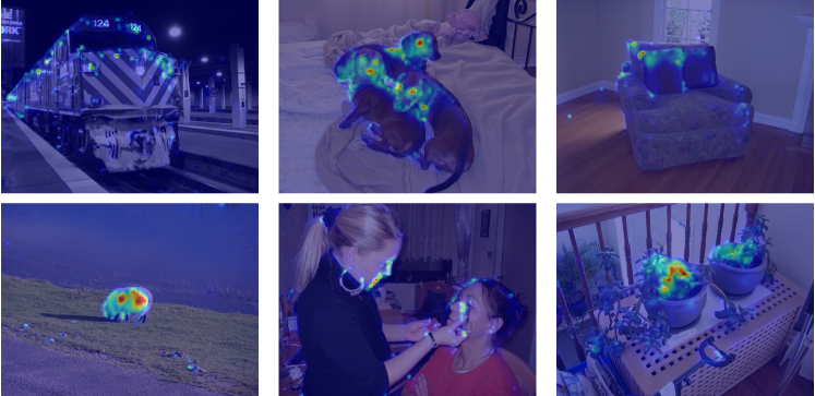
Figure 5: The attention maps of GLM.

Cross Entropy Loss for PLM. One of the contributions is providing a novel way to utilize the ignoring areas. As shown in the second row of Table. 3, without the CE, the performance drops drastically from 79.4% to 68.9%. For seen and unseen categories, the performance is also hurt badly, i.e. from 81.0% to 73.0% for seen categories, and 77.8% to 65.3% for unseen categories. This experiment implies the significance of the CE loss.

Global Learning Module. Another contribution of this work is proposing the GLM module to probe knowledge from the CLIP model. The effectiveness of the GLM is shown in the third row of the Table. 3. Note that the $\gamma$ we use in this ablation is 5.0. As depicted, the hIoU drastically drops from 45.4% to 13.2% which is a large performance drop. The huge drop is attributed to the weakness in recognition of unseen categories, i.e., unseen mIoU drops from 50.7% to 8.6%. This ablation study shows learning from CLS tokens strengthens the recognition of unseen categories by a large margin.

In addition, we further visualize the attention maps of GLM during training as shown in Fig. 5. In this figure, train, potted plant, sofa, and sheep are the unseen categories during training. We can find that even if the models have never seen them the model can still find the discriminative parts of the objects for both seen and unseen categories.

Generate Loss for PLM. As shown in the third row of Table. 3, we do not use any explicit loss function to upgrade the parameters of VLA. The performance drop of 0.2% in hIoU. Meanwhile, both the performance of seen and unseen categories are hurt, i.e., 0.1% and 0.2%, respectively. This result indicates explicit loss function is beneficial to our method.

Different design of GLM. GLM is proposed to align the dense features with the CLS tokens from the CLIP model. We compare the self-attention-based design with other forms as shown in Table. 4. In this table, Attention means the original design, max indicates the max pooling in the dense tokens, and mean indicates the average pooling. Our design achieves the highest performance, i.e., 45.4 in hIoU. Compared with max and mean, the performance gain is by a large margin, i.e., 3.4% higher than the mean and 9.9% higher than the max. The experiment proves that considering all the features is a significant way to learn from CLS token.

Different design of PLM. PLM is proposed to take advantage of both seen and ignored areas. We compare the original design with two other designs: an MLP-ReLU-MLP network and directly applying the corresponding features as shown in Table. 5. Compared with the MLP, our design surpasses it by 0.2% hIoU. For the original features, ours outperforms it by 0.3%, which proves the merits of our design.

4.5 Qualitative Results

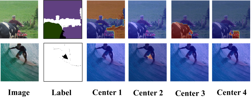
Figure 6: The attention maps of K-Means. In the ‘Label’ column the white area indicates the seen categories, the black area indicates the ignored areas, and other colors imply the unseen categories. The right four images, i.e., Center1-4, indicates the output of the multi-scale K-Means algorithms.

The roles of K-Means algorithms. To further investigate if the dense tokens output by the CLIP visual encoder is highly correlated, we visualize the results of K-Means algorithms as shown in Fig. 6. The white area in the label indicates the seen categories and other areas are unseen. As can be seen from the figure, different centers can group different categories. For example, the area grouped by center 1 indicates the grass. For center 3, the cows can be grouped. It is noticeable that in center 4, a category (maybe tractor) that is not annotated can also be grouped, and the same thing can be observed in center 2. This ablation proves the effectiveness of the multi-scale K-Means algorithms.

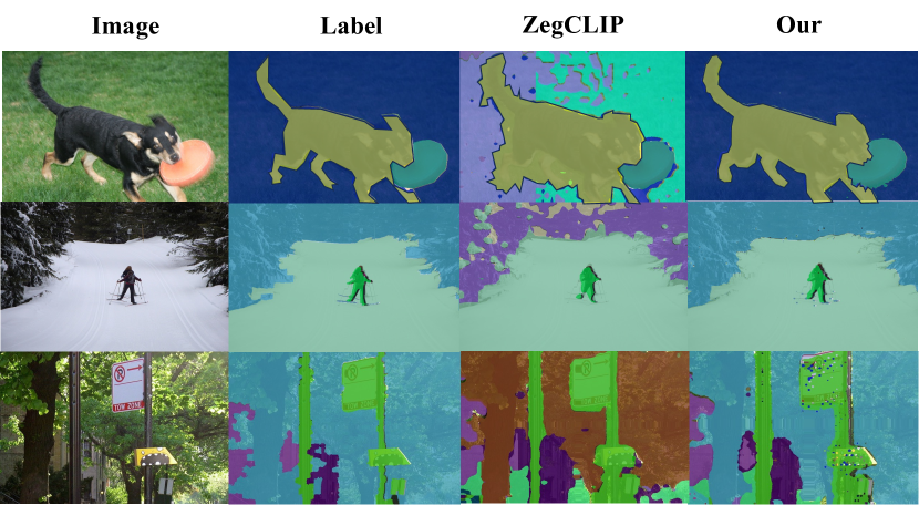
Figure 7: The visualization of the prediction.

The visualization of prediction. We visualize the prediction of our methods as shown in Fig. 7. Our method can obtain exceptional results on both seen and unseen categories (frisbee, tree, grass) trained on only seen categories.

5 Conclusion and Limitations

In this paper, we propose CLIPTeacher, a new framework that releases the VLM-based GZLSS models from the fixed backbones, i.e., ViT or ResNet, and effectively utilizes both the seen and ignoring areas without introducing any change to the vanilla CLIP model. Specifically, CLIPTeacher consists of two key modules: Global Learning Module (GLM) and Pixel Learning Module (PLM). GLM is proposed to directly probe knowledge from the CLS token in the CLIP model which is the only token trained in the CLIP visual encoder. PLM can fully take advantage of the input images on both seen and ignored areas rather than only the seen categories without introducing any extra parameters.

However, there are still limitations in our models. The K-Means algorithm in PLM sometimes can not perfectly distinguish between extremely similar categories, e.g., grass, and tree. Moreover, the weight for the ignoring areas is simply produced by a transformer decoder, which may need more careful designs to improve the qualities. Meanwhile, different from the existing methods that can directly use the self-training [47, 55, 3, 54] strategies to be applied in transductive setting, our method still needs redesign the self-training strategy to be applied in transductive settings.

References

- [1] Radhakrishna Achanta, Appu Shaji, Kevin Smith, Aurelien Lucchi, Pascal Fua, and Sabine Süsstrunk. Slic superpixels compared to state-of-the-art superpixel methods. IEEE transactions on pattern analysis and machine intelligence, 34(11):2274–2282, 2012.
- [2] Donghyeon Baek, Youngmin Oh, and Bumsub Ham. Exploiting a joint embedding space for generalized zero-shot semantic segmentation. In Proceedings of the IEEE/CVF international conference on computer vision, pages 9536–9545, 2021.
- [3] Maxime Bucher, Tuan-Hung Vu, Matthieu Cord, and Patrick Pérez. Zero-shot semantic segmentation. Advances in Neural Information Processing Systems, 32, 2019.
- [4] Mathilde Caron, Hugo Touvron, Ishan Misra, Hervé Jégou, Julien Mairal, Piotr Bojanowski, and Armand Joulin. Emerging properties in self-supervised vision transformers. In Proceedings of the IEEE/CVF international conference on computer vision, pages 9650–9660, 2021.
- [5] Liang-Chieh Chen, George Papandreou, Iasonas Kokkinos, Kevin Murphy, and Alan L Yuille. Deeplab: Semantic image segmentation with deep convolutional nets, atrous convolution, and fully connected crfs. IEEE transactions on pattern analysis and machine intelligence, 40(4):834–848, 2017.
- [6] Liang-Chieh Chen, Yukun Zhu, George Papandreou, Florian Schroff, and Hartwig Adam. Encoder-decoder with atrous separable convolution for semantic image segmentation. In Proceedings of the European conference on computer vision (ECCV), pages 801–818, 2018.
- [7] Ting Chen, Simon Kornblith, Mohammad Norouzi, and Geoffrey Hinton. A simple framework for contrastive learning of visual representations. In International conference on machine learning, pages 1597–1607. PMLR, 2020.
- [8] Ting Chen, Simon Kornblith, Kevin Swersky, Mohammad Norouzi, and Geoffrey E Hinton. Big self-supervised models are strong semi-supervised learners. Advances in neural information processing systems, 33:22243–22255, 2020.
- [9] Xinlei Chen, Haoqi Fan, Ross Girshick, and Kaiming He. Improved baselines with momentum contrastive learning. arXiv preprint arXiv:2003.04297, 2020.
- [10] Bowen Cheng, Ishan Misra, Alexander G Schwing, Alexander Kirillov, and Rohit Girdhar. Masked-attention mask transformer for universal image segmentation. In Proceedings of the IEEE/CVF conference on computer vision and pattern recognition, pages 1290–1299, 2022.
- [11] Bowen Cheng, Alex Schwing, and Alexander Kirillov. Per-pixel classification is not all you need for semantic segmentation. Advances in Neural Information Processing Systems, 34:17864–17875, 2021.
- [12] Jiaxin Cheng, Soumyaroop Nandi, Prem Natarajan, and Wael Abd-Almageed. Sign: Spatial-information incorporated generative network for generalized zero-shot semantic segmentation. In Proceedings of the IEEE/CVF International Conference on Computer Vision, pages 9556–9566, 2021.
- [13] MMSegmentation Contributors. Mmsegmentation: Openmmlab semantic segmentation toolbox and benchmark, 2020.
- [14] Marius Cordts, Mohamed Omran, Sebastian Ramos, Timo Rehfeld, Markus Enzweiler, Rodrigo Benenson, Uwe Franke, Stefan Roth, and Bernt Schiele. The cityscapes dataset for semantic urban scene understanding. In Proceedings of the IEEE conference on computer vision and pattern recognition, pages 3213–3223, 2016.
- [15] Jifeng Dai, Haozhi Qi, Yuwen Xiong, Yi Li, Guodong Zhang, Han Hu, and Yichen Wei. Deformable convolutional networks. In Proceedings of the IEEE international conference on computer vision, pages 764–773, 2017.
- [16] Jian Ding, Nan Xue, Gui-Song Xia, and Dengxin Dai. Decoupling zero-shot semantic segmentation. In Proceedings of the IEEE/CVF Conference on Computer Vision and Pattern Recognition, pages 11583–11592, 2022.
- [17] Zheng Ding, Jieke Wang, and Zhuowen Tu. Open-vocabulary panoptic segmentation with maskclip. arXiv preprint arXiv:2208.08984, 2022.
- [18] Alexey Dosovitskiy, Lucas Beyer, Alexander Kolesnikov, Dirk Weissenborn, Xiaohua Zhai, Thomas Unterthiner, Mostafa Dehghani, Matthias Minderer, Georg Heigold, Sylvain Gelly, et al. An image is worth 16x16 words: Transformers for image recognition at scale. arXiv preprint arXiv:2010.11929, 2020.
- [19] Golnaz Ghiasi, Xiuye Gu, Yin Cui, and Tsung-Yi Lin. Scaling open-vocabulary image segmentation with image-level labels. In European Conference on Computer Vision, pages 540–557. Springer, 2022.
- [20] Zhangxuan Gu, Siyuan Zhou, Li Niu, Zihan Zhao, and Liqing Zhang. Context-aware feature generation for zero-shot semantic segmentation. In Proceedings of the 28th ACM International Conference on Multimedia, pages 1921–1929, 2020.
- [21] Jie Guo, Qimeng Wang, Yan Gao, Xiaolong Jiang, Xu Tang, Yao Hu, and Baochang Zhang. Mvp-seg: Multi-view prompt learning for open-vocabulary semantic segmentation. arXiv preprint arXiv:2304.06957, 2023.
- [22] Meng-Hao Guo, Cheng-Ze Lu, Qibin Hou, Zhengning Liu, Ming-Ming Cheng, and Shi-Min Hu. Segnext: Rethinking convolutional attention design for semantic segmentation. Advances in Neural Information Processing Systems, 35:1140–1156, 2022.
- [23] Mark Hamilton, Zhoutong Zhang, Bharath Hariharan, Noah Snavely, and William T Freeman. Unsupervised semantic segmentation by distilling feature correspondences. arXiv preprint arXiv:2203.08414, 2022.
- [24] Cong Han, Yujie Zhong, Dengjie Li, Kai Han, and Lin Ma. Zero-shot semantic segmentation with decoupled one-pass network. arXiv preprint arXiv:2304.01198, 2023.
- [25] Kaiming He, Haoqi Fan, Yuxin Wu, Saining Xie, and Ross Girshick. Momentum contrast for unsupervised visual representation learning. In Proceedings of the IEEE/CVF conference on computer vision and pattern recognition, pages 9729–9738, 2020.
- [26] Kaiming He, Xiangyu Zhang, Shaoqing Ren, and Jian Sun. Deep residual learning for image recognition. In Proceedings of the IEEE conference on computer vision and pattern recognition, pages 770–778, 2016.
- [27] Neil Houlsby, Andrei Giurgiu, Stanislaw Jastrzebski, Bruna Morrone, Quentin De Laroussilhe, Andrea Gesmundo, Mona Attariyan, and Sylvain Gelly. Parameter-efficient transfer learning for nlp. In International Conference on Machine Learning, pages 2790–2799. PMLR, 2019.
- [28] Chao Jia, Yinfei Yang, Ye Xia, Yi-Ting Chen, Zarana Parekh, Hieu Pham, Quoc Le, Yun-Hsuan Sung, Zhen Li, and Tom Duerig. Scaling up visual and vision-language representation learning with noisy text supervision. In International conference on machine learning, pages 4904–4916. PMLR, 2021.
- [29] Menglin Jia, Luming Tang, Bor-Chun Chen, Claire Cardie, Serge Belongie, Bharath Hariharan, and Ser-Nam Lim. Visual prompt tuning. In European Conference on Computer Vision, pages 709–727. Springer, 2022.
- [30] Boyi Li, Kilian Q. Weinberger, Serge Belongie, Vladlen Koltun, and René Ranftl. Language-driven semantic segmentation, 2022.
- [31] Tsung-Yi Lin, Priya Goyal, Ross Girshick, Kaiming He, and Piotr Dollár. Focal loss for dense object detection. In Proceedings of the IEEE international conference on computer vision, pages 2980–2988, 2017.
- [32] Ze Liu, Yutong Lin, Yue Cao, Han Hu, Yixuan Wei, Zheng Zhang, Stephen Lin, and Baining Guo. Swin transformer: Hierarchical vision transformer using shifted windows. In Proceedings of the IEEE/CVF international conference on computer vision, pages 10012–10022, 2021.
- [33] Zhuang Liu, Hanzi Mao, Chao-Yuan Wu, Christoph Feichtenhofer, Trevor Darrell, and Saining Xie. A convnet for the 2020s. In Proceedings of the IEEE/CVF Conference on Computer Vision and Pattern Recognition, pages 11976–11986, 2022.
- [34] Jonathan Long, Evan Shelhamer, and Trevor Darrell. Fully convolutional networks for semantic segmentation. In Proceedings of the IEEE conference on computer vision and pattern recognition, pages 3431–3440, 2015.
- [35] Jishnu Mukhoti, Tsung-Yu Lin, Omid Poursaeed, Rui Wang, Ashish Shah, Philip HS Torr, and Ser-Nam Lim. Open vocabulary semantic segmentation with patch aligned contrastive learning. In Proceedings of the IEEE/CVF Conference on Computer Vision and Pattern Recognition, pages 19413–19423, 2023.
- [36] Aaron van den Oord, Yazhe Li, and Oriol Vinyals. Representation learning with contrastive predictive coding. arXiv preprint arXiv:1807.03748, 2018.
- [37] Maxime Oquab, Timothée Darcet, Theo Moutakanni, Huy V. Vo, Marc Szafraniec, Vasil Khalidov, Pierre Fernandez, Daniel Haziza, Francisco Massa, Alaaeldin El-Nouby, Russell Howes, Po-Yao Huang, Hu Xu, Vasu Sharma, Shang-Wen Li, Wojciech Galuba, Mike Rabbat, Mido Assran, Nicolas Ballas, Gabriel Synnaeve, Ishan Misra, Herve Jegou, Julien Mairal, Patrick Labatut, Armand Joulin, and Piotr Bojanowski. Dinov2: Learning robust visual features without supervision, 2023.
- [38] Adam Paszke, Sam Gross, Francisco Massa, Adam Lerer, James Bradbury, Gregory Chanan, Trevor Killeen, Zeming Lin, Natalia Gimelshein, Luca Antiga, et al. Pytorch: An imperative style, high-performance deep learning library. Advances in neural information processing systems, 32, 2019.
- [39] Jie Qin, Jie Wu, Pengxiang Yan, Ming Li, Ren Yuxi, Xuefeng Xiao, Yitong Wang, Rui Wang, Shilei Wen, Xin Pan, et al. Freeseg: Unified, universal and open-vocabulary image segmentation. In Proceedings of the IEEE/CVF Conference on Computer Vision and Pattern Recognition, pages 19446–19455, 2023.
- [40] Alec Radford, Jong Wook Kim, Chris Hallacy, Aditya Ramesh, Gabriel Goh, Sandhini Agarwal, Girish Sastry, Amanda Askell, Pamela Mishkin, Jack Clark, et al. Learning transferable visual models from natural language supervision. In International conference on machine learning, pages 8748–8763. PMLR, 2021.
- [41] Gyungin Shin, Weidi Xie, and Samuel Albanie. Namedmask: Distilling segmenters from complementary foundation models. In Proceedings of the IEEE/CVF Conference on Computer Vision and Pattern Recognition, pages 4960–4969, 2023.
- [42] Christian Szegedy, Wei Liu, Yangqing Jia, Pierre Sermanet, Scott Reed, Dragomir Anguelov, Dumitru Erhan, Vincent Vanhoucke, and Andrew Rabinovich. Going deeper with convolutions. In Proceedings of the IEEE conference on computer vision and pattern recognition, pages 1–9, 2015.
- [43] Zhi Tian, Chunhua Shen, Hao Chen, and Tong He. Fcos: Fully convolutional one-stage object detection. In Proceedings of the IEEE/CVF International Conference on Computer Vision (ICCV), October 2019.
- [44] Ashish Vaswani, Noam Shazeer, Niki Parmar, Jakob Uszkoreit, Llion Jones, Aidan N Gomez, Łukasz Kaiser, and Illia Polosukhin. Attention is all you need. Advances in neural information processing systems, 30, 2017.
- [45] Xiaolong Wang, Ross Girshick, Abhinav Gupta, and Kaiming He. Non-local neural networks. In Proceedings of the IEEE conference on computer vision and pattern recognition, pages 7794–7803, 2018.
- [46] Zhirong Wu, Yuanjun Xiong, Stella X Yu, and Dahua Lin. Unsupervised feature learning via non-parametric instance discrimination. In Proceedings of the IEEE conference on computer vision and pattern recognition, pages 3733–3742, 2018.
- [47] Yongqin Xian, Subhabrata Choudhury, Yang He, Bernt Schiele, and Zeynep Akata. Semantic projection network for zero-and few-label semantic segmentation. In Proceedings of the IEEE/CVF Conference on Computer Vision and Pattern Recognition, pages 8256–8265, 2019.
- [48] Yongqin Xian, Subhabrata Choudhury, Yang He, Bernt Schiele, and Zeynep Akata. Semantic projection network for zero-and few-label semantic segmentation. In Proceedings of the IEEE/CVF Conference on Computer Vision and Pattern Recognition, pages 8256–8265, 2019.
- [49] Enze Xie, Wenhai Wang, Zhiding Yu, Anima Anandkumar, Jose M Alvarez, and Ping Luo. Segformer: Simple and efficient design for semantic segmentation with transformers. Advances in Neural Information Processing Systems, 34, 2021.
- [50] Mengde Xu, Zheng Zhang, Fangyun Wei, Han Hu, and Xiang Bai. Side adapter network for open-vocabulary semantic segmentation. In Proceedings of the IEEE/CVF Conference on Computer Vision and Pattern Recognition, pages 2945–2954, 2023.
- [51] Mengde Xu, Zheng Zhang, Fangyun Wei, Yutong Lin, Yue Cao, Han Hu, and Xiang Bai. A simple baseline for open-vocabulary semantic segmentation with pre-trained vision-language model. In European Conference on Computer Vision, pages 736–753. Springer, 2022.
- [52] Youcai Zhang, Xinyu Huang, Jinyu Ma, Zhaoyang Li, Zhaochuan Luo, Yanchun Xie, Yuzhuo Qin, Tong Luo, Yaqian Li, Shilong Liu, et al. Recognize anything: A strong image tagging model. arXiv preprint arXiv:2306.03514, 2023.
- [53] Sixiao Zheng, Jiachen Lu, Hengshuang Zhao, Xiatian Zhu, Zekun Luo, Yabiao Wang, Yanwei Fu, Jianfeng Feng, Tao Xiang, Philip HS Torr, et al. Rethinking semantic segmentation from a sequence-to-sequence perspective with transformers. In Proceedings of the IEEE/CVF conference on computer vision and pattern recognition, pages 6881–6890, 2021.
- [54] Chong Zhou, Chen Change Loy, and Bo Dai. Extract free dense labels from clip. In European Conference on Computer Vision, pages 696–712. Springer, 2022.
- [55] Ziqin Zhou, Yinjie Lei, Bowen Zhang, Lingqiao Liu, and Yifan Liu. Zegclip: Towards adapting clip for zero-shot semantic segmentation. In Proceedings of the IEEE/CVF Conference on Computer Vision and Pattern Recognition, pages 11175–11185, 2023.