ARRQP: Anomaly Resilient Real-time QoS Prediction Framework with Graph Convolution

Abstract

In the realm of modern service-oriented architecture, ensuring Quality of Service (QoS) is of paramount importance. The ability to predict QoS values in advance empowers users to make informed decisions, ensuring that the chosen service aligns with their expectations. This harmonizes seamlessly with the core objective of service recommendation, which is to adeptly steer users towards services tailored to their distinct requirements and preferences. However, achieving accurate and real-time QoS predictions in the presence of various issues and anomalies, including outliers, data sparsity, grey sheep instances, and cold start scenarios, remains a challenge. Current state-of-the-art methods often fall short when addressing these issues simultaneously, resulting in performance degradation. In response, in this paper, we introduce an anomaly-resilient real-time QoS prediction framework (called ARRQP). Our primary contributions encompass proposing an innovative approach to QoS prediction aimed at enhancing prediction accuracy, with a specific emphasis on improving resilience to anomalies in the data. ARRQP utilizes the power of graph convolution techniques, a powerful tool in graph-based machine learning, to capture intricate relationships and dependencies among users and services. By leveraging graph convolution, our framework enhances its ability to model and seize complex relationships within the data, even when the data is limited or sparse. ARRQP integrates both contextual information and collaborative insights, enabling a comprehensive understanding of user-service interactions. By utilizing robust loss functions, this approach effectively reduces the impact of outliers during the training of the predictive model. Additionally, we introduce a method for detecting grey sheep users or services that is resilient to sparsity. These grey sheep instances are subsequently treated separately for QoS prediction. Furthermore, we address the cold start problem as a distinct challenge by emphasizing contextual features over collaborative features. This approach allows us to effectively handle situations where newly introduced users or services lack historical data. Experimental results on the publicly available benchmark WS-DREAM dataset demonstrate the framework’s effectiveness in achieving accurate and timely QoS predictions, even in scenarios where anomalies abound.

1 Introduction

In today’s service-oriented digital landscape, ensuring Quality of Service (QoS) is a critical imperative. QoS prediction [1], the process of forecasting service performance, is indispensable for users and systems to make informed decisions. However, this task is riddled with challenges, including data sparsity, the cold start problem, the presence of outliers, and grey sheep instances.

Collaborative filtering (CF) [2] has emerged as a highly promising solution for QoS prediction. However, early CF-based methods [3, 4, 5, 6], which rely on exploring the similarity of users/services, suffer from low prediction accuracy due to their lack of consideration for data anomalies.

Despite some advancements using low-rank matrix factorization [7, 8, 9, 10, 11, 12] and factorization machines [13, 14, 15] to tackle data sparsity, the cold start problem, and scalability, these methods frequently encounter challenges in achieving satisfactory performance. This is primarily because they have limited capacity to capture higher-order features and are incapable of handling various other anomalies such as grey sheep [16] and outliers [8] present in QoS data.

Among recent advancements on QoS prediction, learning-based methods [17, 18, 19, 20, 21, 22, 23, 24, 25, 8, 26] are particularly notable for their performance improvement, as they excel in capturing the complex features of users and services. Nevertheless, the learning-based methods that heavily rely on contextual features [18, 27, 28, 29, 30] for QoS prediction may struggle to achieve desirable prediction accuracy when collaborative QoS features, which are often more relevant, are absent or not adequately considered. To further enhance prediction accuracy, recent techniques in the literature have aimed to address anomalies in QoS prediction, including handling outliers using robust outlier-resilient loss functions [31, 32, 25, 8, 22] and addressing the cold start problem [33]. However, many of these methods tend to focus on a subset of these challenges and may fall short when multiple issues coexist simultaneously, leading to performance degradation. Consequently, there is a pressing need for an innovative approach that not only enhances prediction accuracy but also bolsters resilience to anomalies in the data, which is the primary objective of this paper.

Our earlier work on QoS prediction [23] introduced a graph-based solution to mitigate the issue of sparsity but did not address other challenges. The present research is an extension of our earlier work. Here, we not only enhance our predictive model but also prioritize the resolution of other anomalies, including outliers, the cold start problem, and the presence of grey sheep instances. Consequently, we have attained a substantial improvement in both prediction time and accuracy compared to our earlier work.

In this paper, we propose a scalable, real-time QoS prediction framework (ARRQP) that effectively addresses multiple anomalies, including outliers, data sparsity, grey sheep instances, and cold start, ultimately enhancing prediction accuracy. Our proposed framework consists of five key components: two anomaly detection blocks responsible for identifying grey sheep users/services and outliers, and three prediction blocks. The first prediction block is engineered to withstand outliers and data sparsity for regular users and services. The other two prediction blocks are specifically dedicated to predicting QoS for grey sheep users/services and newly added users/services that lack sufficient data. The primary contributions of this paper are outlined as follows:

• We propose a multi-layer multi-head graph convolution matrix factorization (MhGCMF) model complemented by an outlier-resilient loss function. This model is designed to capture the intricate relationships among QoS data, effectively mitigating the influence of outliers. It not only enhances prediction accuracy but also ensures minimal prediction time, making it a valuable addition to QoS prediction methodologies.

• The synergy between contextual and QoS features, in addition to the spatial features automatically extracted by MhGCMF, significantly enhances the model’s expressiveness in capturing the complex, higher-order association between user and services. This enhancement eventually leads to improved prediction performance.

• We introduce a sparsity-resilient method for detecting grey sheep users or services.

• Grey sheep instances possess unique characteristics, making it challenging to predict QoS values for such users or services using collaborative filtering alone. Consequently, we have devised a distinct QoS prediction model specifically tailored to address grey sheep users or services. This model incorporates a quantitative distinction measure obtained from the grey sheep detection block, allowing us to provide more accurate predictions for this particular category of users or services.

• We address the cold start problem by designing a separate model that prioritizes contextual features over collaborative features.

• We conducted comprehensive experiments using the benchmark WS-DREAM RT and TP datasets [34] to assess the effectiveness of each block within ARRQP, as well as to evaluate the overall performance of ARRQP.

The rest of the paper is organized as follows. Section 2 presents an overview of the problem with its formulation. Section 3 then discusses the proposed solution framework in detail. The experimental results are analyzed in Section 4, while the literature review is presented in Section 5. Finally, Section 6 concludes this paper.

2 Overview and Problem Formulation

In this section, we discuss an overview of the QoS prediction problem followed by our problem formulation. We are given:

• A set of $n$ users ${\mathcal{U}}$

• Contextual information $\mathcal{C}^{u}$ of each $u\in{\mathcal{U}}$, this contextual information includes user id, user region, autonomous system, etc.

• A set of $m$ web services ${\mathcal{S}}$

• Contextual information $\mathcal{C}^{s}$ of each $s\in{\mathcal{S}}$, where contextual information comprises service id, service region, service provider, etc.

• A QoS parameter $q$

• A QoS log matrix $\mathcal{Q}$ of dimension $n\times m$ containing past user-service interactions in terms of $q$, as defined:

  $$\mathcal{Q}=\begin{cases}q_{ij}\in\mathbb{R}_{>0},&\text{value of $q$ of $s_{j}$ invoked by $u_{i}$}\\ 0,&\text{otherwise}\end{cases}$$ (1)

Each non-zero entry ($q_{ij}\neq 0$) in the matrix represents the value of $q$ of $s_{j}$ invoked by $u_{i}$. Zero entries, on the other hand, denote no interactions between user-service. It may be noted that the QoS log matrix is, in general, a sparse matrix.

The objective of the QoS prediction problem is to predict the QoS value of a given target user-service pair $u_{i}$ and $s_{j}$, where $q_{ij}=0$. In general, the classical QoS prediction problem aims to reduce the prediction error as much as possible. However, minimizing the prediction error is challenging due to the following:

• Data sparsity problem (${\mathds{S}}$): As we discussed earlier, the QoS log matrix is highly sparse. Therefore, minimizing the prediction error while predicting a missing value in the presence of other missing values is a challenging task.

• Presence of outliers (${\mathds{O}}$): The presence of outliers in the QoS log matrix impedes minimizing the prediction error. Therefore, identifying and handling the outliers is essential to meet the objective.

• Presence of grey sheep users/services (${\mathds{GS}}$): The grey sheep users/services are the ones having unique QoS invocation patterns in terms of $q$. Therefore, predicting the QoS values of the grey sheep users/services as compared to the other users/services is difficult.

• Cold-start problem (${\mathds{C}}$): This is the situation when new users/services have been added to the system. Due to the absence of any past data, it is difficult to predict the QoS values of the new users/services.

Objective: This paper aims to design a real-time and scalable QoS prediction framework by addressing the above challenges to attain reasonably low prediction error.

3 Methodology

In this section, we discuss our framework, ARRQP, for QoS prediction. ARRQP comprises two major anomaly detection blocks: (a) Grey sheep user/service Detection block (GD), (b) Outlier Detection block (OD); and three major prediction blocks: (a) Sparsity and Outlier Resilient Real-time QoS Prediction block (SORRQP), (b) Grey sheep users/services Resilient Real-time QoS Prediction block (GRRQP), (c) Cold-start Resilient Real-time QoS Prediction block (CRRQP). In the following subsections, we discuss each of these blocks in detail. We begin with discussing our first prediction block, SORRQP, which primarily deals with sparsity and outliers.

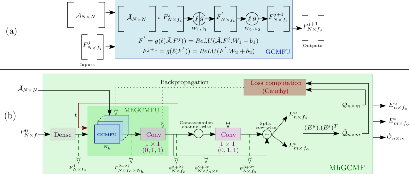
Figure 1: Architecture of SORRQP: (a) Details of GCMFU; (b) Architecture for MhGCMF

3.1 SORRQP Block

SORRQP leverages graph convolution [35] to deal with the data sparsity. The graph convolutional network (GCN) takes privilege in graph architecture and effectively aggregates the node features through message passing between neighboring nodes. Graph architecture has more expressive power [35] than most known representations of users and services. Therefore, in this paper, we adopt graph convolution as the fundamental operation in the SORRQP architecture. Here, we propose a multi-layer multi-head graph convolution matrix factorization (MhGCMF) model for QoS prediction. Fig. 1 shows the overview of SORRQP architecture. Before discussing the further details of MhGCMF, we first define the QoS Invocation Graph (QIG), which is a basic building block of graph convolution operation.

Definition 3.1 (QoS Invocation Graph (QIG)).

A QIG, $\mathcal{G}$ = ($V_{1}\cup V_{2}$, $E$, ${\mathcal{E}}_{1}\cup{\mathcal{E}}_{2}$) is a bipartite graph, where $V_{1}$ and $V_{2}$ are the set of vertices representing the set of users and services, respectively. An edge $e_{ij}=(v_{i}^{1}\in V_{1},v_{j}^{2}\in V_{2})\in E$ exists in $\mathcal{G}$ if $q_{ij}\neq 0$ in the QoS log matrix ${\mathcal{Q}}$. ${\mathcal{E}}_{1}$ and ${\mathcal{E}}_{2}$ represent the set of feature embedding for each node in $V_{1}$ and $V_{2}$, respectively. $\blacksquare$

We now illustrate the details of the feature embedding used in this paper.

3.1.1 Construction of the Feature Embedding

Our initial feature embedding comprises a set of QoS features along with a set of contextual features. We now briefly discuss the details of this embedding.

QoS features: The QoS features include three different types of features, which are discussed below.

(i) Statistical features (${\mathcal{F}}^{u}_{t},{\mathcal{F}}^{s}_{t}$): To capture the self characteristics of each user $u_{i}$ and service $s_{j}$, we compute 5 statistical features, as shown in Table I. It may be noted that since ${\mathcal{Q}}(i)$ is a partially filled QoS invocation vector (QIV), the data sparsity affects the statistical features.

TABLE I: Feature embedding for QIG

$min^{u}_{i}:min({\mathcal{Q}}(i))$	$min^{s}_{j}:min({\mathcal{Q}}^{T}(j))$
$max^{u}_{i}:max({\mathcal{Q}}(i))$	$max^{s}_{j}:max({\mathcal{Q}}^{T}(j))$
$\mu^{u}_{i}:mean({\mathcal{Q}}(i))$	$\mu^{s}_{j}:mean({\mathcal{Q}}^{T}(j))$
$med^{u}_{i}:median({\mathcal{Q}}(i))$	$med^{s}_{j}:median({\mathcal{Q}}^{T}(j))$
$\sigma^{u}_{i}:std\_dev({\mathcal{Q}}(i))$	$\sigma^{s}_{j}:std\_dev({\mathcal{Q}}^{T}(j))$
$std\_dev:$ standard deviation
${\mathcal{Q}}(i)$: $i^{th}$ row of ${\mathcal{Q}}$; ${\mathcal{Q}}^{T}$: Transpose of ${\mathcal{Q}}$

(ii) Collaborative features (${\mathcal{F}}_{n}^{u},{\mathcal{F}}_{n}^{s}$): They are derived from the QoS log matrix. We perform non-negative matrix decomposition [7] of ${\mathcal{Q}}$ to obtain the collaborative QoS features of $u_{i}$ and $s_{j}$, each with dimension $d_{n}$.

(iii) Similarity features (${\mathcal{F}}_{s}^{u},{\mathcal{F}}_{s}^{s}$): They are also extracted from the QoS log matrix. We employ the cosine similarity metric (CSM) to obtain the similarity between pairwise users $(u_{i},u_{k})$ and services $(s_{j},s_{k})$, computed as:

$$CSM(u_{i},u_{k})=\dfrac{{\mathcal{Q}}(i)\cdot{\mathcal{Q}}(k)}{\left\|{\mathcal{Q}}(i)\right\|_{2}\left\|{\mathcal{Q}}(k)\right\|_{2}}$$ (2)

$$CSM(s_{j},s_{k})=\dfrac{{\mathcal{Q}}^{T}(j)\cdot{\mathcal{Q}}^{T}(k)}{\left\|{\mathcal{Q}}^{T}(j)\right\|_{2}\left\|{\mathcal{Q}}^{T}(k)\right\|_{2}}$$ (3)

It is worth noting that the similarity between two users/services is 0 if they do not have any common invocations. Therefore, in general, the similarity features remain sparse due to the sparsity of ${\mathcal{Q}}$. Furthermore, depending on the number of users and services, the similarity feature vector may be a high-dimensional vector. It may be noted that the length of the similarity feature vector for each user $u_{i}$ and service $s_{j}$ are $n$ and $m$, respectively. Therefore, we employ two different auto-encoders [36] for the users and services separately to obtain the low-dimensional similarity feature vector of length $d_{s}$.

Contextual features (${\mathcal{F}}_{c}^{u},{\mathcal{F}}_{c}^{s}$): We utilize the contextual information associated with each $u_{i}$ and $s_{j}$ to prepare the contextual features. The user contextual features include the user ID, region, and autonomous system (AS) information, whereas the service contextual features comprise the service ID, service region, and service provider information. We use the one-hot encoding for each contextual information. Here again, the dimension of the feature vector becomes large due to the high number of users and services. Therefore, we employ auto-encoders to obtain the contextual feature vector of length $d_{c}$.

Finally, all the above feature vectors are concatenated to construct the feature embedding ${\mathcal{E}}^{i}_{1}=({\mathcal{F}}_{t}^{<u,i>}||{\mathcal{F}}_{n}^{<u,i>}||{\mathcal{F}}_{s}^{<u,i>}||{\mathcal{F}}_{c}^{<u,i>})\in{\mathcal{E}}_{1}$ and ${\mathcal{E}}^{j}_{2}=({\mathcal{F}}_{t}^{<s,j>}||{\mathcal{F}}_{n}^{<s,j>}||{\mathcal{F}}_{s}^{<s,j>}||{\mathcal{F}}_{c}^{<s,j>})\in{\mathcal{E}}_{2}$ for each user $u_{i}$ and service $s_{j}$, respectively. Here, ${\mathcal{F}}_{t}^{<u,i>}$ refers to the statistical features for $u_{i}$. The rest of them are denoted similarly. The length of the initial feature embedding (say, $f$) for each user/service is, therefore, $(5+d_{n}+d_{s}+d_{c})$. The initial feature embedding matrix $F^{0}$ is defined in Eq. 4.

$$F^{0}=(\rho^{0}_{ij})\in\mathbb{Z}^{N\times f};\rho^{0}_{i}=\begin{cases}{\mathcal{E}}^{i}_{1}\in{\mathbb{R}}^{f},\text{ if }i\leq n\\ {\mathcal{E}}^{i-n}_{2}\in{\mathbb{R}}^{f},~{}\text{otherwise}\end{cases}$$ (4)

The contextual features are less proficient than QoS features in capturing the intricate relationship among users and services, particularly in the context of QoS prediction. However, relying solely on QoS features often results in lower accuracy due to the sparse nature of the QoS log matrix. Therefore, in this paper, we combine both types of features to create the initial feature embedding. In addition to the initial feature embedding, we incorporate spatial collaborative features obtained from the MhGCMF, which forms the core component of SORRQP. The graph architecture in the MhGCMF enables each user/service to integrate the neighbor information into its embedding, resulting in richer representations that facilitate effective QoS prediction. We now discuss the details of MhGCMF. The primary goal of the MhGMCF is to learn the spatial features from the initial feature embedding of the users and services, with the aim of enhancing the efficiency of QoS prediction. The GCMF Unit (GCMFU) is the central component for MhGCMF. Therefore, we begin with explaining the GCMFU.

3.1.2 Architecture of GCMFU

GCMFU aggregates the neighborhood features of a node $v_{i}^{k}\in(V_{1}\cup V_{2}),~{}k\in\{1,2\}$ from its neighbors, as modeled by the two equations shown in Fig. 1(a). Here, we leverage the adjacency matrix representation of $\mathcal{G}$ to aggregate the neighborhood features. To preserve the self features of each node in the aggregation, we additionally make the diagonal entries of the adjacency matrix as 1. The modified adjacency matrix $\mathcal{A}\in\mathbb{R}^{N\times N}$ is defined in Eq. 5.

$$\small\mathcal{A}=(a_{ij})\in\{0,1\}^{N\times N};a_{ij}=\begin{cases}1,~{}\text{if }i~{}=~{}j\text{ or }e_{ij}\in E\\ 0,~{}\text{otherwise}\end{cases}$$ (5)

Where, $N=n+m$. We then normalize $\mathcal{A}$, as shown in Eq. 6, to avoid the scaling discrepancy caused by the varying degrees of the nodes in $\mathcal{G}$ because of the sparsity of $\mathcal{Q}$ and generate $\bar{\mathcal{A}}$. The diagonal degree matrix ($\mathcal{D}$), as defined in Eq. 7, is used for the normalization. The normalization reduces the impact of the higher degree nodes in QoS prediction.

$$\small\bar{\mathcal{A}}=\mathcal{D}^{-1/2}~{}\mathcal{A}~{}\mathcal{D}^{-1/2}\\$$ (6)

$$\mathcal{D}=(d_{ij})\in\mathbb{Z}^{N\times N};~{}~{}d_{ij}=\begin{cases}\sum\limits_{k=1}^{N}{\mathcal{A}}(i,k),\text{ if }i=j\\ 0,~{}\text{otherwise}\end{cases}$$ (7)

The GCMFU receives $\bar{\mathcal{A}}$ and a feature embedding matrix (say, $F^{j}$) as its input. It then performs a non-linear transformation on $F^{j}$ with the help of a set of learnable parameters (refer to Fig. 1(a)) and produces the updated feature embedding matrix (say, $F^{j+1}$) by incorporating the spatial information of the neighborhood nodes. We now discuss the detailed architecture of the MhGCMF.

3.1.3 Architecture of MhGCMF

Fig. 1(b) summarizes the architecture of the MhGCMF. Given the normalized adjacency matrix $\bar{\mathcal{A}}$ and the initial feature embedding matrix $F^{0}$, the objective of the MhGCMF is to learn the spatial collaborative features for each user/service and predict the QoS value of a given user-service pair.

In MhGCMF, $F^{0}$ first undergoes an initial transformation by passing through a dense layer, resulting in the transformed feature embedding $F^{1}$. Subsequently, $F^{1}$ and $\bar{\mathcal{A}}$ are directed to the multi-head GCMFU (i.e., MhGCMFU) block. MhGCMFU comprises $N_{h}$ number of GCMFUs followed by a $1\times 1$ convolution layer. The “multi-head” in MhGCMFU refers to the presence of multiple GCMFUs. The outputs of these multiple GCMFUs are then concatenated channel-wise, and the resulting tensor passes through a $1\times 1$ convolutional layer. This entire process is repeated $t$ times, where the output of MhGCMFU is fed back into itself. The output generated by each MhGCMFU block is once again concatenated channel-wise and then forwarded to another $1\times 1$ convolutional layer. For each $1\times 1$ convolutional layer, there is a corresponding tuple indicating (padding, stride, and number of filters), as illustrated in Fig. 1(b). The output of the final $1\times 1$ convolutional layer is split row-wise to produce the user and service embedding matrices. These matrices are subsequently multiplied to generate the predicted QoS log matrix. We train the MhGCMF for each user-service pair $(u_{i},s_{j})\in\mathcal{U}\times\mathcal{S}$, such that $q_{ij}\neq 0$ using Cauchy Loss Function, as shown in Eq. 8.

$$\small\mathcal{C_{L}}=\sum_{q_{ij}\neq 0}\ln{(1+\frac{||q_{ij}-\hat{q}_{ij}||^{2}}{\gamma^{2}})}$$ (8)

where $\gamma$ is a hyper-parameter that can be tuned externally, and $\hat{q}_{ij}$ is the predicted QoS value. The outlier resilience characteristics of the Cauchy loss function ensure that SORRQP also exhibits outlier resilience. However, SORRQP alone cannot address the other issues, such as grey sheep and cold start. In the next section, we address the issue of grey sheep.

3.2 Grey sheep Detection Block (GD)

Collaborative Filtering (CF) highly relies on the collaborative relationship between users and services and operates on the premise that similar users and services exist within the system. However, it is worth noting that there can be a small group of users or services with QoS patterns that deviate from the norm, making them distinct from the majority. These users and services are often referred to as grey sheep, representing an anomalous subset within the user or service community. The existence of grey sheep users or services may occasionally lead to substantial inaccuracies in QoS predictions. In this context, our approach begins with addressing the task of identifying grey sheep Users/Services (GSU/GSS). Subsequently, we tackle the challenge of QoS prediction for these identified GSUs and/or GSSs. The GD block within ARRQP primarily focuses on identifying the instances of grey sheep within the QoS data.

To capture the distinct QoS pattern exhibited by a user/service, here, we introduce two concepts: reliability score and Grey sheep Anomaly (GA) score [16] for each user/service. These two scores together aid in determining whether a particular user/service qualifies as a GSU/GSS.

Definition 3.2 (Reliability Score).

The reliability score of a user $u_{i}\in\mathcal{U}$ and service $s_{j}\in{\mathcal{S}}$, denoted by $\mathscr{R}(u_{i})$ and $\mathscr{R}(s_{j})$, respectively, are defined as:

$${\mathscr{R}}(u_{i})=$$ (9)

$$1-\left(\frac{\sigma^{u}_{i}-\min\limits_{u_{k}\in{\mathcal{U}}}(\sigma^{u}_{k})}{\max\limits_{u_{k}\in{\mathcal{U}}}(\sigma^{u}_{k})-\min\limits_{u_{k}\in{\mathcal{U}}}(\sigma^{u}_{k})}\right);$$

$${\mathscr{R}}(s_{j})=$$ (10)

$$1-\left(\frac{\sigma^{s}_{j}-\min\limits_{s_{k}\in{\mathcal{S}}}(\sigma^{s}_{k})}{\max\limits_{s_{k}\in{\mathcal{S}}}(\sigma^{s}_{k})-\min\limits_{s_{k}\in{\mathcal{S}}}(\sigma^{s}_{k})}\right)$$

$\sigma^{u}_{i}$ and $\sigma^{s}_{j}$ represent the standard deviation of the QIVs of $u_{i}$ and $s_{j}$, respectively (refer to Table I). $\blacksquare$

It may be noted from Eq.s 9 and 10 that a user/service is said to be more reliable than another if the standard deviation of the QIV of the former is lower than that of the later. We now define GA score in Definition 3.3.

Definition 3.3 (Grey sheep Anomaly (GA) Score).

The GA score of a user $u_{i}\in\mathcal{U}$ and service $s_{j}\in{\mathcal{S}}$, denoted by $\mathscr{G}(u_{i})$ and $\mathscr{G}(s_{j})$, respectively, are defined as:

$$\scriptsize\mathscr{G}(u_{i})=\left({\sum\limits_{s_{j}\in{\mathcal{S}}_{i}}\Bigl{(}|q_{ij}-\mu^{u}_{i}-\bar{\mu}^{s}_{j}|\times{\mathscr{R}}(s_{j})\Bigr{)}}\right)/{|{\mathcal{S}}_{i}|}$$ (11)

$$\scriptsize\mathscr{G}(s_{j})=\left({\sum\limits_{u_{i}\in{\mathcal{U}}_{j}}\Bigl{(}|q_{ij}-\mu^{s}_{j}-\bar{\mu}^{u}_{i}|\times{\mathscr{R}}(u_{i})\Bigr{)}}\right)/{|{\mathcal{U}}_{j}|}$$ (12)

$$\scriptsize\bar{\mu}^{s}_{j}=\left({\left(\sum\limits_{u_{i}\in{\mathcal{U}}_{j}}q_{ij}\right)-\max\limits_{u_{i}\in{\mathcal{U}}_{j}}(q_{ij})-\min\limits_{u_{i}\in{\mathcal{U}}_{j}}(q_{ij})}\right)/\left({|{\mathcal{U}}_{j}|-2}\right)$$ (13)

$\bar{\mu}^{u}_{i}$ is also defined similarly. ${\mathcal{S}}_{i}$ be the set of services invoked by $u_{i}$. ${\mathcal{U}}_{j}$ be the set of users invoked $s_{j}$. $\mu^{u}_{i}$ and $\mu^{s}_{j}$ represent the mean of the QIVs of $u_{i}$ and $s_{j}$, respectively. $\blacksquare$

It may be noted from the above equations that the GA score of each user $u_{i}$ (service $s_{j}$) is computed over its respective QIV, denoted by ${\mathcal{Q}}(i)$ (${\mathcal{Q}}^{T}(j)$). For each invocation $q_{ij}$ ($\neq 0$) made by $u_{i}$ (for $s_{j}$), we compute the deviation with respect to the mean of QIV of $u_{i}$ ($s_{j}$) and centralized mean of $s_{j}$ ($u_{i}$). The average of these weighted deviations, computed over the QIV of $u_{i}$ ($s_{j}$), is referred to as the GA score of $u_{i}$ ($s_{j}$). The reliability score of the corresponding service is used as the weight in this computation. Notably, if a service has a high reliability score, the corresponding deviation carries more weight than one associated with a service with a lower-reliability score. It may be noted the GA score of a user only depends on the set of services it invoked. Therefore, the GA score is not affected by the data sparsity.

We now define the Grey sheep user (GSU) and service (GSS) below.

Definition 3.4 (Grey sheep user (GSU)).

A user $u_{i}\in{\cal{U}}$ (service $s_{j}\in{\cal{S}}$) is called GSU (GSS), if ${\mathscr{G}}(u_{i})$ (${\mathscr{G}}(s_{j})$) is more than a given threshold ${\tau}_{\mathscr{G}}^{u}$ (${\tau}_{\mathscr{G}}^{s}$). $\blacksquare$

${\tau}_{\mathscr{G}}^{u}$ and ${\tau}_{\mathscr{G}}^{s}$ are hyper-parameters. In this paper, we consider ${\tau}_{\mathscr{G}}^{u}=\mu_{\mathscr{G}}^{u}+c*\sigma_{\mathscr{G}}^{u}$ (${\tau}_{\mathscr{G}}^{s}=\mu_{\mathscr{G}}^{s}+c*\sigma_{\mathscr{G}}^{s}$), where $\mu_{\mathscr{G}}^{u}$ and $\sigma_{\mathscr{G}}^{u}$ ($\mu_{\mathscr{G}}^{s}$ and $\sigma_{\mathscr{G}}^{s}$) are the mean and standard deviation of the GA scores of users (services), respectively. $c$ is a hyper-parameter, which can be tuned externally.

Once the GD block identifies the GSU/GSS, the next step involves predicting the QoS values for these identified GSUs/GSSs using our next prediction block, GRRQP. In the following section, we discuss the specifics of the GRRQP.

3.3 GRRQP Block

The GRRQP is primarily designed to provide QoS predictions for GSS/GSU. The rationale behind introducing the GRRQP block stems from the recognition that grey sheep users/services exhibit markedly distinct QoS patterns compared to the majority of users/services. Consequently, relying extensively on collaborative features, as employed in SORRQP, may not be adequate for achieving higher QoS predictions for GSU/GSS. Furthermore, the prediction of QoS values for GSU/GSS in conjunction with other users/services may not be advisable, given that GSU/GSS possess distinct characteristics that set them apart from the rest. Therefore, here, we design separate architectures for the QoS prediction tailored specifically for GSU/GSS.

The GRRQP is an improvisation of SORRQP, featuring supplementary MLPs (Multi-Layer Perceptrons) in addition to the MhGCMF model discussed previously. Here, we have three MLPs designed specifically for (a) non-grey sheep users and GSSs, (b) GSUs and non-grey sheep services, and (c) GSUs and GSSs. The feature vector for each MLP is constructed by concatenating the user features and the service features. If the user $u_{i}$ is a non-grey sheep user, the embedding vector $E^{u}_{i}$ (i.e., $i^{th}$ row of $E^{u}$) obtained from MhGCMF is used as its features. However, if $u_{i}$ is a grey sheep user, its feature is generated by concatenating the following components: (i) the embedding vector $E^{u}_{i}$ obtained from MhGCMF, (ii) the initial feature embedding vector ${\mathcal{E}}_{1}^{i}$, (iii) the GA score ${\mathscr{G}}(u_{i})$, and (iv) the number of invocations of $u_{i}$. The service features are also generated similarly. The MLPs are trained for the user-service pair in the respective categories for which $q_{ij}\neq 0$.

In the following subsection, we illustrate our final prediction block, designed to handle the cold start issue.

3.4 CRRQP Block

The term cold start pertains to a scenario in which a new user/service is introduced into a system. This situation poses a significant challenge for QoS prediction due to the lack of available data. The SORRQP system is ill-suited to handle the cold start scenario for the following reasons: (a) The similarity and statistical features in the initial feature embedding cannot provide meaningful information for the newly added user/service due to the absence of historical data. (b) The newly introduced user/service forms an isolated node within the QIG, indicating no interactions among other users/services. These isolated nodes lack the ability to capture spatial features effectively. As a result, this limitation poses a challenge for SORRQP in making accurate predictions under such circumstances. Therefore, we propose another prediction block, CRRQP, to address the above issue. CRRQP is an enhancement over SORRQP.

In addition to MhGCMF, CRRQP is also equipped with three MLPs to predict the QoS of the following target user-service pairs. (a) Cold Start User (CSU): Here, the target user is new. However, the service has sufficient past data. (b) Cold Start Service (CSS): In this case, the target service is new, while the user has historical data. (a) Cold Start user/service Both (CSB): This scenario involves both the user and service being newly introduced entities without any historical data available for either of them.

The three MLPs are trained separately with three different sets of input features. The input features are constructed by concatenating the user and the service features. If the user/service $u_{i}$/$s_{j}$ is not a newly added, the embedding vector $E^{u}_{i}$/$E^{s}_{j}$ obtained from MhGCMF is used as its features. However, if $u_{i}$/$s_{j}$ is newly added, its feature is generated by concatenating its contextual features and the collaborative features obtained using non-negative matrix decomposition.

In the next subsection, we discuss our final block for outlier detection.

3.5 Outlier Detection Block

In this paper, we employ an unsupervised learning algorithm based on the isolation forest ($i$Forest) algorithm [37] to detect the outliers from scratch. $i$Forest algorithm explicitly isolates the outliers rather than profiling the inliers converse to the distance or density-based approaches for the outliers detection. The strength of the $i$Forest approach is its effectiveness over different benchmarks and high scalability. It uses an ensemble of isolation trees ($i$Tree), whose branch grows iteratively; this way, it isolates every single data point. Finally, in each $i$Tree, the outliers are instances that are isolated near the root of the tree and have comparatively short average path lengths, consecutively, inliers isolated to the far end of the $i$Tree. After identifying the outliers, we proceed to eliminate them from the dataset, with the ratio of removed outliers denoted by $\lambda$ (e.g., $\lambda=0.1$ refers to 10% of the total dataset considered as the outlier). This step is essential to evaluate the performance of our framework without outliers.

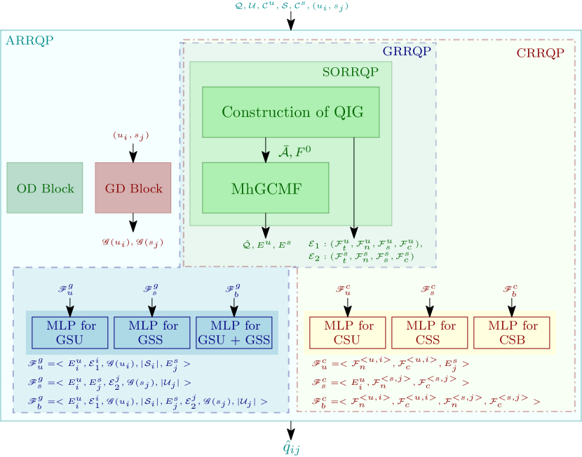
Figure 2: Overall architecture ARRQP

Fig. 2 shows the overall architecture of ARRQP. In the next section, we analyze the performance of ARRQP.

4 Experimental Results

In this section, we present the experimental analysis of our framework. We implemented our proposed framework in TensorFlow 2.6.2 with Python 3.6.9. All experiments were executed on the Linux-5.4.0-133-generic-x86_64-with-Ubuntu-18.04-bionic with Intel(R) Core(TM) i9-10885H CPU @ 2.40GHz x86_64 architecture, 16 Core(s), 128 GB RAM, with the following cache L1d: 32K, L1i:32K, L2:256K, L3:16384K.

4.1 Experimental Setup

In this subsection, we present a comprehensive overview of the datasets, performance metrics, model configurations utilized to conduct our experiment, and finally, the experimental analysis. We begin by detailing the datasets used in our study.

4.1.1 Datasets

We used the benchmark and publicly available WS-DREAM [34] datasets. The dataset contains two different QoS parameters: response time (RT) and throughput (TP). Table II comprehensively provides the details of the dataset.

TABLE II: WS-DREAM datasets details for RT and TP

Statistics	RT	TP
Number of Users	$339$
Number of User’s Regions	$31$
Number of User’s AS	$137$
Number of Services	$5825$
Number of Service’s Regions	$74$
Number of Service’s Providers	$2699$
Number of Valid Invocations	$1873838$	$1831253$
Range (min-max)	$0.0010-19.9990$	$0.0040-1000$
Mean	$0.9086$	$47.5617$
Median	$0.3200$	$13.9530$
Standard Deviation	$1.9727$	$110.7970$

TABLE III: Performance of ARRQP on Response Time (RT)

Anomaly	Methods	MAE				RMSE
Addressed		RT-5	RT-10	RT-15	RT-20	RT-5	RT-10	RT-15	RT-20
None	UPCC [38]	0.7695	0.7201	0.6521	0.5921	1.6940	1.6101	1.4959	1.3993
	IPCC [39]	0.7326	0.7125	0.6783	0.6503	1.6346	1.5439	1.4104	1.3109
	WSRec [3]	0.6794	0.6211	0.6037	0.6020	1.4884	1.4265	1.3684	1.3515
	$\mathcal{I}$ (%)	46.46	49.49	54.16	56.32	16.83	19.69	20.51	23.41
${\mathds{S}}+{\mathds{C}}$	SN-MF [40]	0.6318	0.5377	0.5008	0.4871	1.3968	1.2695	1.2264	1.2073
	LACF [41]	0.6299	0.5601	0.5102	0.4774	1.4399	1.3377	1.2694	1.2220
	NMF [7]	0.6182	0.6040	0.5990	0.5982	1.5746	1.5494	1.5345	1.5531
	LFM [42]	0.5783	0.5644	0.5438	0.5350	1.5010	1.3201	1.2719	1.2269
	LE-MF [43]	0.5734	0.5136	0.4827	0.4646	1.3703	1.2511	1.2041	1.1809
	PMF [44]	0.5678	0.4996	0.4720	0.4492	1.4735	1.2866	1.2163	1.1828
	NIMF [9]	0.5514	0.4884	0.4534	0.4357	1.4075	1.2745	1.1980	1.1678
	LN-LFM [45]	0.5501	0.4889	0.4611	0.4424	1.3145	1.2368	1.2073	1.1568
	RSNMF [46]	0.5438	0.4868	0.4492	0.4371	1.4032	1.2689	1.2067	1.1568
	LBR [29]	0.5389	0.5292	0.5180	0.4941	1.4130	1.3481	1.3260	1.3147
	NAMF [47]	0.5384	0.4850	0.4529	0.4350	1.3850	1.2592	1.2071	1.1443
	GeoMF [33]	0.5305	0.4827	0.4495	0.4366	1.3152	1.2190	1.1742	1.1528
	CNMF [48]	0.5289	0.4713	0.4316	0.4136	1.3053	1.2373	1.1360	1.1161
	CSMF [12]	0.5286	0.4557	0.4225	0.4180	1.3473	1.2315	1.1780	1.1210
	LMF-PP [49]	0.5285	0.4725	0.4472	0.4260	1.3410	1.2419	1.2102	1.1625
	JCF [50]	0.5132	0.4665	0.4504	0.4365	1.3328	1.2505	1.1854	1.1802
	NDMF [51]	0.4880	0.4304	0.3845	0.3665	1.3495	1.2349	1.1569	1.1294
	EFMPred [15]	0.4460	0.3750	0.3630	0.3480	1.3530	1.2810	1.2530	1.2360
	MSDAE [30]	0.4267	0.3640	0.3434	0.3275	1.2853	1.2436	1.1695	1.1283
	LAFIL [28]	0.3880	0.3664	0.3460	0.3268	1.2674	1.1926	1.1106	1.0923
	$\mathcal{I}$ (%)	6.26	13.82	19.42	22.58	2.32	3.94	2.06	8.95
${\mathds{S}}+{\mathds{C}}+{\mathds{O}}$	DCALF [52]	0.5127	0.4544	0.4346	0.4246	1.3731	1.2450	1.2001	1.1759
	NCF [53]	0.4400	0.3850	0.3720	0.3620	1.3250	1.2830	1.2530	1.2050
	SPP+LLMF [54]	0.4350	0.3700	0.3550	0.3360	1.3340	1.2500	1.1920	1.1740
	DNM [27]	0.4125	0.3726	0.3678	0.3575	1.3463	1.2673	1.2490	1.2298
	LDCF [25]	0.4020	0.3670	0.3450	0.3310	1.2770	1.2330	1.1690	1.1380
	DCLG [32]	0.3850	0.3460	0.3260	0.3140	1.2630	1.1850	1.1430	1.1200
	HSA-Net [22]	0.3670	0.3270	0.3070	0.2950	1.2490	1.1660	1.1260	1.0910
	$\mathcal{I}$ (%)	0.90	4.06	9.86	14.24	0.89	1.75	3.40	8.85
${\mathds{S}}+{\mathds{GS}}+{\mathds{O}}+{\mathds{C}}$	ARRQP	0.3637	0.3137	0.2767	0.2530	1.2379	1.1456	1.0877	0.9945
* Improvement of ARRQP over the second-best method highlighted in blue

TABLE IV: Performance of ARRQP on Throughput (TP)

Anomaly	Methods	MAE				RMSE
Addressed		TP-5	TP-10	TP-15	TP-20	TP-5	TP-10	TP-15	TP-20
None	UPCC	27.5760	23.0130	20.6800	19.2940	63.7540	56.6210	51.9550	47.6510
	IPCC	26.8640	26.0590	25.8790	24.2610	65.7900	61.1320	59.1500	54.6970
	WSRec	26.7330	22.6940	20.5470	18.9640	63.4980	56.4590	51.7890	46.9510
	$\mathcal{I}$ (%)	50.40	52.53	52.50	53.97	36.53	34.39	32.48	29.73
${\mathds{S}}+{\mathds{C}}$	CSMF [12]	28.3060	26.5850	25.6250	21.7420	72.7040	70.0210	68.6180	61.6790
	LBR [29]	26.1610	21.0060	18.5840	16.5510	68.0310	57.7280	54.4410	51.6790
	NMF [7]	25.7529	17.8411	15.8939	15.2516	65.8517	53.9896	51.7322	48.6330
	GeoMF [33]	24.7465	22.4728	17.7908	16.2852	57.7842	49.2456	45.3255	43.9545
	LACF [41]	22.9737	19.4489	17.5887	16.4580	58.7857	52.9270	49.5650	47.4108
	RSNMF [46]	21.4302	17.2305	14.6880	14.3654	60.7994	50.5298	45.2647	43.5822
	PMF [44]	19.9034	16.1755	15.0956	14.6694	54.0508	46.4439	43.7957	42.4855
	LB-FM [55]	19.8460	17.4610	17.0460	15.8390	73.8420	65.6800	67.0930	61.8030
	LRMF [56]	19.1090	15.9494	14.5974	13.9206	58.0719	48.2718	44.0682	41.7880
	LN-LFM [45]	18.6512	16.0634	14.7664	14.1264	52.4326	46.8756	44.3871	43.0892
	LMF-PP [49]	18.3091	15.9125	14.7450	14.1033	51.7765	46.1418	42.9927	41.4084
	NAMF [47]	18.0836	15.9808	14.6661	13.9386	52.8658	44.0788	43.0206	40.7481
	NIMF [9]	17.9297	16.0542	14.4363	13.7099	51.6573	45.9409	43.1596	41.1689
	NDMF [51]	16.3818	13.9317	12.5043	11.7204	50.9612	43.9095	42.5319	39.9431
	LAFIL [28]	13.9875	12.2119	11.3761	10.9294	48.5321	42.5069	40.2270	38.6575
	$\mathcal{I}$ (%)	14.77	11.79	14.20	20.13	16.96	12.85	13.89	14.66
${\mathds{S}}+{\mathds{C}}+{\mathds{O}}$	DNM [27]	18.4903	16.2861	15.1406	14.7933	63.2993	55.0821	49.3940	48.4284
	DCALF [52]	17.6576	15.3595	14.3936	13.6697	51.4123	45.9013	42.6235	41.2194
	NCF [53]	15.4680	13.6160	12.2840	11.8330	49.7030	46.3040	42.3170	41.2630
	SPP+LLMF [54]	15.3820	13.6540	11.9040	11.0890	51.5660	45.6810	41.6310	39.5340
	LDCF [25]	13.8440	12.3820	11.2700	10.8410	47.3590	43.4820	39.8130	38.9980
	DCLG [32]	12.9280	11.3040	10.4060	9.9360	43.9690	39.9600	37.6370	36.1760
	$\mathcal{I}$ (%)	-1.97	4.70	6.20	12.15	8.34	7.30	7.97	8.80
${\mathds{S}}+{\mathds{GS}}+{\mathds{O}}+{\mathds{C}}$	ARRQP	13.1839	10.7723	9.7604	8.7285	40.3005	37.0415	34.9693	32.9910
* Improvement of ARRQP over the second best method highlighted in blue

4.1.2 Comparison Metric

To measure the performance of our framework, we used two performance metrics: Mean Absolute Error (MAE) and Root Mean Squared Error (RMSE) defined as follows:

$$MAE=\frac{1}{|TD|}\sum_{(u_{i},s_{j})\in TD}|q_{ij}-{\hat{q}}_{ij}|$$ (14)

and

$$RMSE=\sqrt{\frac{1}{|TD|}\sum_{(u_{i},s_{j})\in TD}(q_{ij}-{\hat{q}}_{ij})^{2}}$$ (15)

where $TD$ is the test dataset and $|TD|$ denotes the size of the test dataset. $q_{ij}$ and ${\hat{q}}_{ij}$ represent the actual and the predicted QoS values of a user-service pair $(u_{i},s_{j})$, respectively.

In general, MAE is the average of non-negative differences between the actual and predicted sample that usually provides equal weight to all the samples. However, RMSE measures a quadratic score which gives relatively high weight to large errors.

Furthermore, we used another measure, called Improvement, to show the performance improvement of our framework over the past methods, which is defined below.

Definition 4.1 (Improvement $I(M_{1},M_{2})$).

Given two error values $P_{1}$ and $P_{2}$ (measured in terms of MAE or RMSE) obtained by two different methods $M_{1}$ and $M_{2}$, respectively, the improvement of $M_{1}$ over $M_{2}$ is defined as: $\blacksquare$

$${\mathcal{I}}(M_{1},M_{2})=\left(({P_{2}-P_{1}})/{P_{2}}\right)\times 100\%$$ (16)

4.1.3 Parameter Configurations

To validate the performance of ARRQP, we used four different training-testing split-ups: $(5\%,95\%),(10\%,90\%),(15\%,85\%),(20\%,80\%)$. In this paper, we use the notation RT-$x$ (TP-$x$) to denote the training-testing split up for $\left(x\%,(100-x)\%\right)$. In other words, for RT-$x$, we used $x\%$ data of the given response time values for training, while the rest was used for testing. Moreover, we used 20% of the training data as the validation dataset for our experiment. We repeated each experiment 10 times and reported the average value.

In all our experiments, unless specifically stated otherwise, we maintained consistent usage of the parameters with values as listed in Table V.

TABLE V: Details of various parameters used in experiments

Parameters	RT-5	RT-10	RT-15	RT-20	TP-5	TP-10	TP-15	TP-20
c, $\lambda$, t	2, 0.1, 2
$d_{n},d_{s},d_{c}$	50, 50, 50
$N_{h}$     MAE	5	1	4	3	5	4	5	5
RMSE	5	1	2	2	5	7	8	6
$\gamma$        MAE	0.05	0.25	0.25	0.25	10	10	50	10
RMSE	250	10	100	10	10	50	50	100

4.2 Experimental Results

We now present the analysis of our experimental results.

4.2.1 Comparison with State-of-the-Art Methods

We compared ARRQP with 30 and 24 major State-of-the-Art (SoA) methods on RT and TP datasets, respectively. Tables III and IV show the performance of ARRQP on RT and TP datasets for different training densities in terms of prediction accuracy, respectively. We have the following observations about the performance of ARRQP.

• Comparison of prediction accuracy with SoA: As observed from Tables III and IV, the prediction error started decreasing as the methods started handling more anomalies. It is worth noting that ARRQP outperformed the major SoA methods since it addressed more variations of anomalies compared to contemporary methods. The improvements of ARRQP over the other methods for each case (the methods are divided based on the anomalies addressed by them) are shown in the tables in bold.

• Comparison of prediction accuracy between ARRQP and DCLG: It may be noted from Table IV, the performance of ARRQP degraded by $-1.97\%$ compared to DCLG [32] in terms of MAE on TP-5. However, the performance of ARRQP improved by $8.34\%$ for the same in terms of RMSE. This shows that even though ARRQP increased the overall errors compared to DCLG, ARRQP was able to reduce the large prediction errors significantly. For the rest of the other cases, however, ARRQP outperformed DCLG in terms of MAE and RMSE.

• Change of prediction accuracy with training density: As observed from Tables III and IV, the performance of ARRQP improved with the increase in the training density. This is because, as the density increases, the number of neighbors of each node in the QoS prediction graph increases, which allows each user and service to have additional spatial collaborative information in the feature vector.

• Training time of ARRQP: The training of ARRQP is performed in offline mode as discussed in Section 3. The training time for ARRQP varied from 1.8 to 21.75 minutes, depending on the number of heads used in GCMF, which varied from 1 to 8 in our experiments.

• Performance of ARRQP in terms of prediction time: The prediction time for ARRQP (including GRRQP and CRRQP) was in the order of $10^{-6}$ seconds, while the prediction time for SORRQP was in the order of $10^{-9}$ seconds. This difference in prediction time between SORRQP and ARRQP was because of the use of an additional MLP employed in GRRQP and CRRQP. The prediction time of ARRQP was negligible compared to the minimum service response time shown in Table II. The prediction of ARRQP is approximately 10 times faster than the prediction time for TRQP [23], which was in the order of $10^{-5}$ seconds, and it is the best-known among all the methods reported in this paper in terms of prediction time.

In summary, ARRQP achieved better prediction accuracy compared to the major SoA methods with a reasonable learning time and negligible prediction time, enabling it to integrate with a real-time service recommendation system.

We now discuss the performance of ARRQP addressing various anomalies discussed in Section 2.

4.2.2 Performance of ARRQP on Addressing Anomalies

This subsection analyzes various anomaly detection mechanisms used in this paper and the performance of ARRQP in dealing with those anomalies. We begin with discussing the performance of ARRQP handling outliers.

TABLE VI: Performance of SORRQP after removal of outliers

Methods	Anomaly	RT-10		RT-20		TP-10		TP-20
	removed	MAE	RMSE	MAE	RMSE	MAE	RMSE	MAE	RMSE
LLMF[54]	$10\%$	0.4041	0.6120	0.4037	0.6106	16.5509	33.8889	13.1105	27.9648
DALF[57]	$10\%$	0.3955	0.7466	0.3439	0.6779	13.1968	27.8531	11.9619	26.0299
CAP[58]	$10\%$	0.3603	0.6439	0.3521	0.6640	16.4269	32.9558	16.3125	32.9334
TAP[59]	$10\%$	0.3385	0.5512	0.2843	0.4985	22.1419	43.4987	19.8273	40.9533
TRQP [23]	$13\%$	0.2540	-	0.2520	-	10.5760	-	9.5660	-
OffDQ [21]	$15\%$	0.2000	-	0.1800	-	9.1600	-	8.6700	-
CMF[8]	$10\%$	0.1762	0.3705	0.1524	0.3599	8.4573	24.9137	7.2501	20.8927
SORRQP	$10\%$	0.0930	0.3556	0.0794	0.2710	4.9652	18.3332	4.0876	16.6755
$\mathcal{I}$ (%)		47.21	4.02	47.90	24.69	41.29	26.41	43.62	20.18
* Improvement of SORRQP over the second best method highlighted in blue

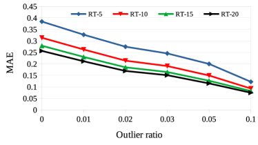
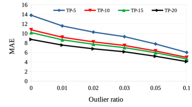
(a)                                          (b)

Figure 3: Analysis of outliers on (a) RT and (b) TP datasets

Impact of Outlier Detection Method: Table VI shows the performance of SORRQP after the removal of 10% outliers (i.e., $\lambda=0.1$). Here, we consider the SoA methods after removing $10\%$ or more data with anomalies, as mentioned in the second column of Table VI. As observed from the final row of Table VI, SORRQP outperformed all the major SoA methods in terms of prediction accuracy by a significant improvement margin.

Fig.s 3 (a) and (b) show the impact of the outlier detection algorithm used in this paper on RT and TP datasets, respectively. Here, we showed the performance of our framework with the removal of $1\%,2\%,3\%,5\%$ and $10\%$ outliers. As observed from Fig.s 3 (a) and (b), the performance of ARRQP (in terms of MAE) improved as more outliers were detected and removed, which shows the efficiency of the outlier detection algorithm.

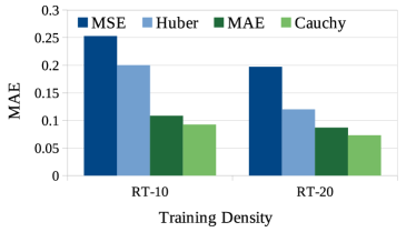
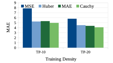
(a)                                          (b)

Figure 4: Analysis of loss functions (a) RT and (b) TP datasets

Impact of Loss Function to Handle Outliers: Fig.s 4(a) and (b) show the impact of the loss functions on the performance of the ARRQP. The MSE is an outlier-sensitive loss function; therefore, it performed worst. MAE, Huber loss and Cauchy loss can deal with the outliers. In our framework, we adopt the Cauchy loss to train our model since it outperformed all other loss functions, as evident from Fig.s 4(a) and (b).

Impact of Grey sheep Detection Algorithm: Fig.s 5 (a) and (b) show the Grey sheep detection capability of GRRQP on RT and TP datasets, respectively. We may infer the following observations from Fig.s 5 (a) and (b) below:

• For $\lambda=0$, as the value of $c$ decreased and the number of detected GSU and GSS increased and removed, the prediction error decreased. Table VII shows the number of detected GSU and GSS for different values of $c$.

• As we removed 10% of the outliers along with the GSU and GSS for every value of $c$, the performance improvement of GRRQP was quite significant compared to the case with removing the GSU and GSS only without removing any outliers.

• For $\lambda=0.1$, the decrease in the prediction error with a decrease in the value of $c$ was not that significant compared to the case for $\lambda=0$. This finding suggests that the presence of a large number of outliers might contribute to the emergence of more grey sheep instances.

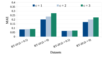
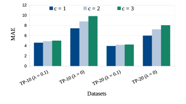
(a)                                          (b)

Figure 5: Analysis of grey sheep detection metric (a) RT and (b) TP datasets

TABLE VII: Number of (GSU, GSS) for different $c$

$c=1$		$c=2$		$c=3$
RT	TP	RT	TP	RT	TP
(35, 254)	(24, 304)	(25, 150)	(7, 233)	(8, 101)	(4, 176)

Performance of GRRQP: Table VIII presents the performance comparison between GRRQP and SORRQP to show the effectiveness of our framework in handling the GSU and GSS. While the SORRQP only addresses sparsity and outliers issues, the GRRQP offers explicit solutions for GSU and GSS in QoS prediction. This experiment was divided into two cases: (i) Case-1: considering all users and GSS $({\mathcal{U}},{\mathcal{S}}_{{\mathcal{G}}})$, (ii) Case-2: considering GSU and all services $({\mathcal{U}}_{{\mathcal{G}}}{,\mathcal{S}})$. The improvement of GRRQP over SORRQP for Case-1 and Case-2 are shown in the last two columns of Table VIII.

TABLE VIII: Performance (MAE) of GRRQP over SORRQP

Dataset	SORRQP		GRRQP		$\mathcal{I}$ (%)
	Case-1	Case-2	Case-1	Case-2	Case-1	Case-2
RT-10	1.7507	0.9278	1.7375	0.8857	0.75	4.54
RT-20	1.4828	0.6441	1.4568	0.5962	1.75	7.44
TP-10	109.3299	23.7551	107.7793	23.2875	1.42	1.97
TP-20	87.4062	20.215	85.8197	19.9767	1.82	1.18

Performance of ARRQP After Grey sheep Removal: Table X demonstrates the performance of ARRQP after removing the data corresponding to GSU and GSS for $c=2$. Here, we compared our framework with the SoA methods that attempted to detect GSU and GSS and produced the results after removing them. As observed from Table X, ARRQP outperformed all the major SoA methods reported in Table X with a significant improvement margin with or without removing outliers.

Moreover, it is worth mentioning that even though the SoA methods attempted to detect GSU and GSS, they failed to handle them. In contrast to the existing literature, ARRQP detects GSU and GSS and effectively handles them.

TABLE IX: Comparison of ARRQP with SoA considering grey sheep removal Methods RT-10 RT-20 TP-10 TP-20 MAE RMSE MAE RMSE MAE RMSE MAE RMSE LRMF [56] 0.4785 1.2576 0.4340 1.1422 - - - - RAP [60] 0.4914 1.4346 0.4531 1.1631 21.4027 - 17.5978 - HLT [61] 0.5088 - 0.3634 - 28.5370 - 22.8296 - CAP [58] 0.4997 - 0.4361 - 16.6465 - 14.2685 - TAP [59] 0.5978 - - - 25.7784 - - - ARRQP 0.2343 1.0106 0.1992 0.9450 8.7754 32.1770 7.2216 28.7231 $\lambda=0.0$ $\mathcal{I}$ (%) 51.03 19.64 45.18 17.26 47.28 - 49.39 - ARRQP 0.2079 0.8180 0.1747 0.7475 8.1668 27.2536 6.7368 24.4762 $\lambda=0.1$ $\mathcal{I}$ (%) 56.55 34.95 51.93 34.56 50.94 - 52.78 - * $\mathcal{I}$ of ARRQP ($c=2$) over the second best method highlighted in blue TABLE X: Comparison of CRRQP with SoA considering the cold start for CSB on RT-10 Methods MAE RMSE $0\%$ $5\%$ $10\%$ $0\%$ $5\%$ $10\%$ GMEAN 1.0154 1.0300 1.0100 1.9678 1.9680 1.9702 USMF [62] 0.5499 0.5800 0.6100 1.4148 1.4954 1.5800 GeoMF1 [33] 0.4890 0.5200 0.5500 1.2022 1.3100 1.4000 GeoMF2 [33] 0.4610 0.5100 0.5200 1.1774 1.2900 1.3800 CRRQP 0.3137 0.3874 0.4479 1.1456 1.2435 1.2905 $\mathcal{I}$ (%) 46.95 31.64 16.09 2.77 3.73 6.93 GMEAN: uses the average QoS value to make predictions

Performance of CRRQP: Cold start scenarios occur when new users or services are added to the system. Therefore, we divided our experiment into three cases as discussed below:

1. CSU: This is the first case where the experiment was designed with a set of cold start users without any data in the system. A cold start percentage (CSP) used for the experiment determines the number of cold start users. The experiment was limited to cold start users and all the services for this case.

2. CSS: This is the second case. Here, the experiment was designed with a set of cold start services having no data in the system. Here CSP also determines the number of cold start services. The experiment was performed on all the users and cold start services for this case.

3. CSB: This is the final case, which combines CSU and CSS. In this case, if the value of CSP is considered as $x$, the $x\%$ of the total users and $x\%$ of the total services are designated as the cold start users and services. The experiment here was performed jointly on all the users with cold start services and cold start users with all the services.

Here, we present the analysis for various values of CSP. Fig.s 6 (a) and (b) show the sensitivity of cold start on the performance of ARRQP on RT and TP datasets, respectively. As evident from Fig.s 6 (a) and (b), the performance of ARRQP deteriorated with the increasing value of CSP. Besides the unavailability of information on cold start users and services, the sparsity caused by the increasing CSP value was another reason for the performance degradation of ARRQP.

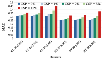
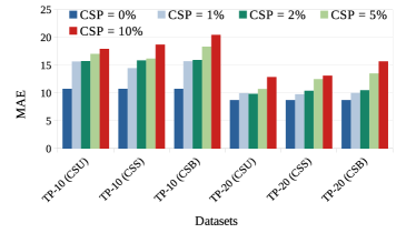
(a)                                          (b)

Figure 6: Analysis of Cold-start on (a) RT and (b) TP datasets

Fig.s 7 (a)–(d) showcase the comparative performance of CRRQP and SORRQP on RT-10, RT-20, TP-10, and TP-20 datasets, respectively. As evident from Fig.s 7(a)–(d), CRRQP consistently outperformed SORRQP, exhibiting a notable average improvement of $18.94\%$ and $7.04\%$ on RT and TP datasets, respectively.

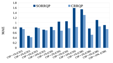
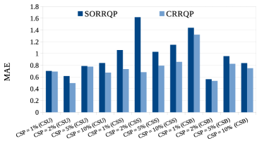
(a)                                          (b)                                 
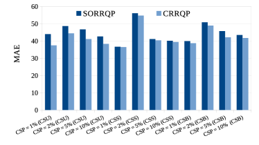
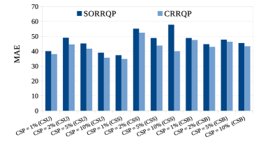
                           (c)                                          (d)

Figure 7: Performance of CRRQP on (a) RT-10, (b) RT-20, (c) TP-10, (d) TP-20 datasets

Table X illustrates the performance of CRRQP compared to SoA methods for CSB with CSP of $0\%$, $5\%$, and $10\%$ on the RT-10 dataset. Table X clearly demonstrates the significant performance enhancement achieved by CRRQP over the existing SoA methods that addressed the cold start problem.

The above studies show the efficiency of ARRQP in handling various anomalies. In the following subsection, we discuss the ablation study for our framework.

4.2.3 Ablation Study

We begin our discussion with the feature ablation study.

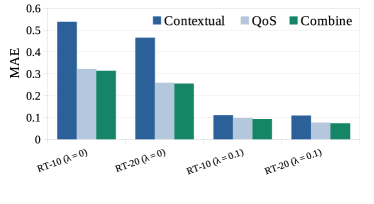
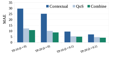
(a)                                          (b)                                 
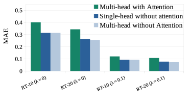
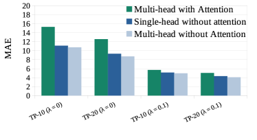
                           (c)                                          (d)

Figure 8: Feature ablation study on (a) RT, (b) TP; Model ablation study on (c) RT, (d) TP datasets

Feature Ablation Study: Fig.s 8 (a) and (b) illustrate the influence of different features used in our framework. From Fig.s 8 (a) and (b), we can infer the following.

• ARRQP with contextual features exhibited the worst performance. Even though the impact of QoS features was more prominent than the impact of the contextual features, however, ARRQP with a combination of contextual and QoS features outperformed the same with only QoS features by $2.01\%$ and $12.63\%$ on RT and TP datasets, respectively, on average.

• For $\lambda=0.1$, all three models showed significant performance improvements compared to the case for $\lambda=0$. The improvement percentages are $78.07\%,70.02\%,70.93\%$ on RT, and $70.21\%,55.75\%,53.49\%$ on TP datasets for ARRQP with contextual features, QoS features and combined features, respectively.

Model Ablation Study: We studied the individual performance of GRRQP and CRRQP as compared to SORRQP in Table VIII and Fig.s 7 (a)–(d), respectively. These results emphasize the importance of GRRQP to handle grey sheep users and services and CRRQP to handle cold start situations in ARRQP alongside SORRQP to handle sparsity and outliers.

4.2.4 Comparative Model Study

Here, we present a comparative study between three models: the single-head without attention model, the multi-head without attention model, and the multi-head with attention model. Fig.s 8 (c) and (d) present the performance of all three models on RT and TP datasets, respectively. The following can be inferred from Fig.s 8 (c) and (d):

• The multi-head without attention model outperformed the multi-head with attention model [63] by an average improvement of $23.69\%$ and $30.08\%$ on RT and TP datasets, respectively. Moreover, it also surpassed the single-head without attention model by an average improvement of $1.34\%$ and $4.74\%$ on RT and TP datasets, respectively.

• A similar trend can be observed after the removal of 10$\%$ outliers.

4.2.5 Impact of Hyper-parameters

In this subsection, we study the influence of various hyper-parameters used in our framework.

Impact of $\gamma$: $\gamma$ is a hyper-parameter present in the Cauchy loss function. Fig.s 9 (a) and (b) illustrate the performance of ARRQP with the change in the value of $\gamma$ on RT and TP datasets, respectively. Among different $\gamma$ values, we observed that $\gamma=0.25$ and $\gamma=10$ achieved the best performance for all training densities on the RT and TP datasets, respectively. The same trend was followed after removing the $10\%$ of outliers from the datasets.

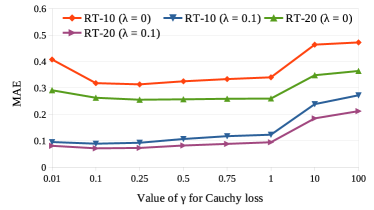
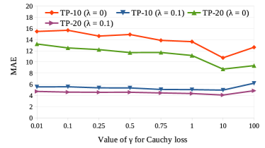
(a)                                          (b)                                 
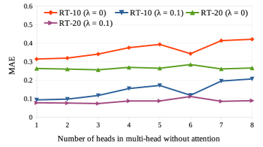
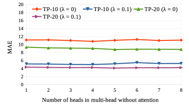
                           (c)                                          (d)

Figure 9: Analysis of $\gamma$ on (a) RT and (b) TP; Analysis of number of heads in multi-head without attention model on (c) RT and (d) TP datasets

Impact of Number of Heads: We tuned our model with different numbers of heads. The experimental results are shown in Fig.s 9 (c) and (d) for the RT and TP datasets, respectively. The following observations may be drawn from the figures:

• For RT datasets, although there is no fixed pattern, one head is sufficient to achieve the best performance at $10\%$ training density, while three heads performed best at $20\%$ training density. Moreover, removing $10\%$ of outliers enhances the model’s performance.

• For TP datasets, the best performance is observed with four heads at 10% training density and five heads at $20\%$ training density.

TABLE XI: Confidence Intervals

CL	RT-5	RT-10	RT-15	RT-20	TP-5	TP-10	TP-15	TP-20
90	(0.3545, 0.3549)	(0.3052, 0.3055)	(0.2661, 0.2664)	(0.2399, 0.2402)	(12.5458, 12.5576)	(10.4042, 10.4152)	(8.8769, 8.8865)	(8.3365, 8.3450)
95	(0.3545, 0.3549)	(0.3051, 0.3055)	(0.2661, 0.2665)	(0.2398, 0.2402)	(12.5447, 12.5587)	(10.4032, 10.4162)	(8.8759, 8.8874)	(8.3357, 8.3458)
99	(0.3544, 0.3550)	(0.3051, 0.3056)	(0.2661, 0.2665)	(0.2398, 0.2402)	(12.5425, 12.5609)	(10.4011, 10.4183)	(8.8741, 8.8892)	(8.3341, 8.3474)

4.2.6 Statistical Significance Testing

To establish the reliability of ARRQP, we assess the statistical significance of our model using confidence intervals (CIs) [64]. A CI essentially provides a range around a measurement, indicating the precision of that measurement. Typically, CIs are computed for various confidence levels (CL), such as $90\%,95\%$, and $99\%$. A $x\%$ CL implies that there is a $(100-x)\%$ chance of uncertainty in the experiments for being wrong.

The insights derived from Table XI enable us to evaluate the error precision of ARRQP under diverse conditions, facilitating well-informed decisions concerning the reliability of ARRQP. Notably, as we move from lower to higher CL, the CI tends to become wider. In summary, this comprehensive analysis strengthens the validity of ARRQP and underscores its practical significance.

5 Related Work

This section presents a concise overview of relevant literature to discuss various anomalies in QoS prediction. In the domain of QoS prediction, Collaborative Filtering (CF) emerges as a widely adopted method. CF-based methods predominantly rely on the collaborative relationships among users and services. They often leverage the similarity between users and/or services as a foundational element to facilitate QoS prediction. However, it is worth noting that CF-based methods often encounter various difficulties, including coping with high data sparsity, addressing cold-start issues, handling outliers, dealing with grey sheep problems, and exploiting intricate relationships among users and services. These challenges eventually result in elevated prediction errors [1, 2]. To address these challenges and enhance QoS prediction accuracy, more advanced techniques have been proposed in the literature. We now discuss various challenges and their possible solutions explored in the literature.

Data Sparsity: Data sparsity is a prevalent challenge in the field of QoS prediction, which occurs due to an insufficient number of interactions between users and services, making it difficult to predict accurate QoS values because of the limited available information. To tackle the sparsity problem, the literature has proposed several solutions, including: (i) Low-rank matrix decomposition: It [7, 8, 11, 44, 54, 40, 46, 12, 9, 51, 50] tackles the sparsity problem by capturing underlying patterns and relationships among users and services by decomposing the user-service interaction matrix into low-dimensional matrices and subsequently reconstructing it. However, while matrix decomposition-based methods are effective in handling sparsity, they encounter additional challenges, such as noise handling or difficulty in capturing higher-order relationships among users/services, potentially leading to inaccuracies in predictions. (ii) Designing additional data imputation method: This is used sometimes to predict the missing values [14, 21, 20, 48]. These imputed values are then utilized by the prediction module to estimate the final QoS value for the target user-service pair. However, the performance of the data imputation method directly affects the quality of predictions. Hence, the chosen data imputation method should be sophisticated to yield accurate results. Nonetheless, employing data imputation adds an extra layer of complexity to the prediction process, which, in turn, may result in reduced scalability and slower responsiveness of the prediction system. (iii) Use of contextual data for prediction: As seen in some approaches [65, 27, 28, 29, 30], leveraging contextual data for prediction can help alleviate sparsity issues in certain cases. However, contextual data is not always readily available. Furthermore, when contextual information is used in isolation without any collaborative QoS data, it becomes challenging to capture the complex relationships between users and services. As a result, prediction accuracy may suffer and degrade.

Presence of Outliers: Outliers are data points that deviate significantly from the majority of the data, introducing anomalies that can hinder the performance of prediction algorithms. In the literature, outliers are predominantly addressed through two distinct approaches. (i) Utilizing outlier-resilient loss functions: Some methods employ specialized loss functions that are resilient to the influence of outliers. These loss functions, such as L1 loss [27, 54, 22], Huber loss [31, 32, 25], Cauchy loss [8, 23], have been demonstrated to be more effective than the standard L2 loss function when dealing with outliers. These robust loss functions downweight the impact of outliers during the training process, allowing the model to focus more on learning from the majority of the data. (i) Detecting and removing outliers: Alternatively, certain methods follow the explicit outliers detection [21, 8, 23, 52] and followed by subsequent removal of them, resulting in a more reliable dataset for the prediction model.

Presence of Grey sheep: Grey sheep users/services refer to those with QoS invocation patterns that are sufficiently different from the others, often characterized by unique underlying behaviors. Therefore, the traditional and intuitive solutions may not effectively address them. The existing methods focus on identifying grey sheep instances and avoiding them. Here are some approaches used to detect the grey sheep. RAP [60] mitigates the data credibility problem by leveraging the user reputation ranking algorithm, which identifies untrustworthy users present in the data. TAP [59] ensures credibility by employing unsupervised K-means clustering with beta distribution to calculate the reputation of users. CAP [58] utilizes a two-phase K-means clustering-based credibility-aware QoS prediction method, where clusters with a minimum number of users are considered untrustworthy. However, despite these efforts, data sparsity remains a significant challenge that can hinder the identification of grey sheep users or services. Sparse data may not provide enough information to accurately distinguish between typical and atypical behaviors, making it challenging to address grey sheep instances effectively.

Moreover, to the best of our knowledge, prediction methods tailored specifically for grey sheep users/services are mostly unexplored in the literature. However, understanding and effectively accommodating these grey sheep users/services in prediction algorithms can be crucial for achieving more accurate and personalized QoS predictions. Cold Start: The term cold start is widely used to describe the scenario when new users or services are introduced to a system [33]. These freshly added users or services typically lack data in the form of invocation history or have minimal associated data, leading to subpar prediction performance. It is important to note that the solutions designed to handle data sparsity are also highly relevant for addressing cold-start scenarios. Techniques developed to mitigate sparsity-related challenges can be adapted to improve predictions for cold-start instances by leveraging available data effectively [41, 45, 47, 15, 51, 9, 28, 29, 43, 30, 25].

Table XII presents a comprehensive summary of the literature on anomaly detection and handling, encompassing 38 SoA methods and our proposed framework. Notably, our framework demonstrates its efficacy in detecting and effectively handling all the mentioned anomalies.

TABLE XII: A brief literature survey on anomaly detection and handling of QoS prediction

Methods	Anomaly Detection		Anomaly Handling
	$\mathds{O}$	$\mathds{GS}$	$\mathds{S}$	$\mathds{O}$	$\mathds{GS}$	$\mathds{C}$
[38, 39, 3]
[7, 44, 40, 41, 42, 43, 9, 45, 46, 29, 62]			✓			✓
[47, 33, 12, 49, 50, 51, 15, 30, 28, 48]
[58, 60, 59]		✓
[21, 8]	✓		✓	✓		✓
[56, 61]		✓	✓			✓
[52]	✓	✓		✓
[54, 27, 25, 32, 22]			✓	✓		✓
[23]	✓	✓	✓	✓		✓
ARRQP	✓	✓	✓	✓	✓	✓

Positioning Our Proposed Work: In contrast to the approaches discussed above, this paper introduces several innovative solutions to mitigate the challenges associated with QoS prediction.

(i)  We propose a simple yet effective solution leveraging graph convolution [35], which excels in dealing with high sparsity by aggregating and sharing neighborhood information of the nodes.

(ii)  Integrating both contextual information and QoS data, along with spatial collaborative information, offers a holistic perspective on user-service interactions here. This comprehensive approach enhances the system’s ability to understand user behaviors and service performance, evidently resulting in more accurate predictions.

(iii)  The outlier-resilient Cauchy loss enables us to minimize the impact of outliers during the model training.

(iv)  The grey sheep detection block in ARRQP empirically shows the effectiveness in identifying grey sheep users/services. Importantly, it has the advantage of being able to handle the issue of data sparsity because it does not rely on measuring similarity between users/services.

(v)  In addition to the above, ARRQP offers an effective model specifically designed for predicting the QoS values of grey sheep users or services.

(vi)  The CRRQP block is specifically designed to address the prediction of QoS for newly added users/services. It recognizes the challenges posed by the cold start scenario, where these newcomers lack historical data, and takes special measures to make accurate predictions despite the limited information available. This specialized attention to cold start situations ensures that ARRQP can provide meaningful QoS predictions even for users or services with minimal or no prior usage history.

In summary, ARRQP demonstrates resilience to anomalies and is a well-suited framework for integration into real-time service recommendation systems, given its high scalability and responsiveness.

6 Conclusion

This paper introduces an anomaly-resilient real-time QoS prediction framework (ARRQP), designed to achieve highly accurate QoS prediction in negligible time by addressing various challenges and anomalies, including the presence of outliers, data sparsity, grey sheep instances, and the cold start problem. ARRQP proposes a multi-head graph convolution matrix factorization model to capture complex relationships and dependencies among users and services. By doing so, it enhances its capacity to predict QoS accurately, even in the face of data limitations. Furthermore, ARRQP integrates contextual information and collaborative insights, enabling a holistic understanding of user-service interactions. Robust loss functions are employed to mitigate the impact of outliers during model training, improving predictive accuracy. In addition to QoS prediction, ARRQP introduces a sparsity-resilient method for detecting grey sheep users or services. These distinctive instances are subsequently handled separately for QoS prediction, ensuring tailored and accurate predictions. Moreover, the cold start problem is addressed as a distinct challenge, emphasizing the importance of contextual features. ARRQP also exhibited a high responsiveness and scalability, rendering it well-suited for integration into real-time systems. This characteristic positions ARRQP as a valuable tool for applications where timely and efficient QoS prediction is essential.

The incorporation of advanced anomaly detection and mitigation algorithms holds promise for enhancing the performance of QoS prediction methods. Additionally, the development of a time-aware extension to ARRQP is a crucial area of focus for our future research endeavors. These directions represent our commitment to advancing the capabilities of QoS prediction and ensuring its relevance in dynamic and evolving systems.

Suraj Kumar is pursuing his PhD in CSE from the IIT Indore, India. He received his B.Tech and M.Tech in CSE from Aligarh Muslim University, India, in 2017 and 2019, respectively. His research interests include Services Computing, Machine Learning, and Graph Representation Learning.

Soumi Chattopadhyay (Member, IEEE) received her Ph.D. from the Indian Statistical Institute in 2019. Currently, she is an Assistant Professor at IIT Indore, India. Her research interests include Services Computing, Artificial Intelligence, Machine Learning, Deep Learning, Formal Languages, Logic and Reasoning.

References

- [1] Z. Zheng et al., “Web service QoS prediction via collaborative filtering: A survey,” IEEE Transactions on Services Computing, vol. 15, no. 4, pp. 2455–2472, 2022.
- [2] S. H. Ghafouri et al., “A survey on web service QoS prediction methods,” IEEE TSC, vol. 15, no. 4, pp. 2439–2454, 2022.
- [3] Z. Zheng et al., “QoS-aware web service recommendation by collaborative filtering,” IEEE TSC, vol. 4, no. 2, pp. 140–152, 2011.
- [4] H. Sun et al., “Personalized web service recommendation via normal recovery collaborative filtering,” IEEE TSC, vol. 6, no. 4, pp. 573–579, 2013.
- [5] G. Zou et al., “QoS-aware web service recommendation with reinforced collaborative filtering,” in ICSOC, vol. 11236, 2018, pp. 430–445.
- [6] X. Wu et al., “Collaborative filtering service recommendation based on a novel similarity computation method,” IEEE TSC, vol. 10, no. 3, pp. 352–365, 2017.
- [7] D. D. Lee et al., “Learning the Parts of Objects by Non-Negative Matrix Factorization,” Nature, vol. 401, no. 6755, p. 788, 1999.
- [8] F. Ye et al., “Outlier-resilient web service QoS prediction,” in WWW, 2021, pp. 3099–3110.
- [9] Z. Zheng et al., “Collaborative web service QoS prediction via neighborhood integrated matrix factorization,” IEEE TSC, vol. 6, no. 3, pp. 289–299, 2013.
- [10] Z. Chen et al., “An accurate and efficient web service QoS prediction model with wide-range awareness,” FGCS, vol. 109, pp. 275–292, 2020.
- [11] W. Lo et al., “An extended matrix factorization approach for QoS prediction in service selection,” in IEEE SCC, 2012, pp. 162–169.
- [12] H. Wu et al., “Collaborative QoS prediction with context-sensitive matrix factorization,” FGCS, vol. 82, pp. 669–678, 2018.
- [13] M. Li et al., “A two-tier service filtering model for web service QoS prediction,” IEEE Access, vol. 8, pp. 221 278–221 287, 2020.
- [14] L. Shen et al., “Contexts enhance accuracy: On modeling context aware deep factorization machine for web API QoS prediction,” IEEE Access, vol. 8, pp. 165 551–165 569, 2020.
- [15] Y. Wu et al., “An embedding based factorization machine approach for web service QoS prediction,” in ICSOC, vol. 10601, 2017, pp. 272–286.
- [16] B. Gras et al., “Identifying Grey Sheep Users in Collaborative Filtering: A Distribution-Based Technique,” in UMAP. ACM, 2016, p. 17–26.
- [17] S. Chattopadhyay and A. Banerjee, “QoS value prediction using a combination of filtering method and neural network regression,” in ICSOC, vol. 11895, 2019, pp. 135–150.
- [18] Y. Yin et al., “QoS prediction for service recommendation with features learning in mobile edge computing environment,” IEEE TCCN, vol. 6, no. 4, pp. 1136–1145, 2020.
- [19] G. Zou et al., “Ncrl: Neighborhood-based collaborative residual learning for adaptive QoS prediction,” IEEE TSC, pp. 1–14, 2022.
- [20] R. R. Chowdhury et al., “CAHPHF: context-aware hierarchical QoS prediction with hybrid filtering,” IEEE TSC, vol. 15, no. 4, pp. 2232–2247, 2022.
- [21] S. Chattopadhyay et al., “OffDQ: An Offline Deep Learning Framework for QoS Prediction,” in WWW. ACM, 2022, p. 1987–1996.
- [22] Z. Wang et al., “Hsa-net: Hidden-state-aware networks for high-precision QoS prediction,” IEEE TPDS, vol. 33, no. 6, pp. 1421–1435, 2022.
- [23] S. Kumar and S. Chattopadhyay, “TRQP: trust-aware real-time QoS prediction framework using graph-based learning,” in ICSOC, vol. 13740, 2022, pp. 143–152.
- [24] J. Li et al., “Topology-aware neural model for highly accurate QoS prediction,” IEEE TPDS, vol. 33, no. 7, pp. 1538–1552, 2022.
- [25] Y. Zhang et al., “Location-aware deep collaborative filtering for service recommendation,” IEEE TSMC, vol. 51, no. 6, pp. 3796–3807, 2021.
- [26] M. I. Smahi et al., “A deep learning approach for collaborative prediction of web serviceQoS,” Serv. Oriented Comput. Appl., vol. 15, no. 1, pp. 5–20, 2021.
- [27] H. Wu et al., “Multiple attributes QoS prediction via deep neural model with contexts,” IEEE TSC, vol. 14: 4, pp. 1084–1096, 2021.
- [28] Z. Wang et al., “Location-aware feature interaction learning for web service recommendation,” in ICWS. IEEE, 2020, pp. 232–239.
- [29] W. Lo et al., “Collaborative Web Service QoS Prediction with Location-Based Regularization,” in IEEE ICWS, 2012, pp. 464–471.
- [30] M. Wu, Q. Lu, and Y. Wang, “A multi-stack denoising autoencoder for QoS prediction,” in ICANN, 2022, pp. 757–768.
- [31] F. R. Hampel et al., Robust statistics: the approach based on influence functions. Wiley-Interscience; New York, 1986.
- [32] Z. Jia et al., “Location-aware web service QoS prediction via deep collaborative filtering,” IEEE TCSS, pp. 1–12, 2022.
- [33] Z. Chen et al., “Your neighbors alleviate cold-start: On geographical neighborhood influence to collaborative web service QoS prediction,” Knowl. Based Syst., vol. 138, pp. 188–201, 2017.
- [34] Z. Zheng et al., “Investigating QoS of real-world web services,” IEEE TSC, vol. 7, no. 1, pp. 32–39, 2014.
- [35] T. N. Kipf and M. Welling, “Semi-supervised classification with graph convolutional networks,” in ICLR, 2017.
- [36] P. Vincent et al., “Stacked denoising autoencoders: Learning useful representations in a deep network with a local denoising criterion,” J. Mach. Learn. Res., vol. 11, p. 3371–3408, dec 2010.
- [37] F. T. Liu et al., “Isolation forest,” in 2008 Eighth IEEE International Conference on Data Mining, 2008, pp. 413–422.
- [38] J. S. Breese et al., “Empirical analysis of predictive algorithms for collaborative filtering,” in UAI. Morgan Kaufmann, 1998, pp. 43–52.
- [39] B. M. Sarwar et al., “Item-based collaborative filtering recommendation algorithms,” in WWW. ACM, 2001, pp. 285–295.
- [40] J. Yin and Y. Xu, “Personalised QoS-based web service recommendation with service neighbourhood-enhanced matrix factorisation,” Int. J. Web Grid Serv., vol. 11, no. 1, pp. 39–56, 2015.
- [41] M. Tang et al., “Location-aware collaborative filtering for QoS-based service recommendation,” in ICWS, 2012, pp. 202–209.
- [42] Y. Koren et al., “Matrix factorization techniques for recommender systems,” Computer, vol. 42, no. 8, pp. 30–37, 2009.
- [43] Y. Xu et al., “Context-aware QoS prediction for web service recommendation and selection,” Expert Syst. Appl., vol. 53, pp. 75–86, 2016.
- [44] R. Salakhutdinov and A. Mnih, “Probabilistic matrix factorization,” in NIPS. Red Hook, NY, USA: Curran Associates Inc., 2007, p. 1257–1264.
- [45] D. Yu et al., “Personalized QoS prediction for web services using latent factor models,” in SCC, 2014, pp. 107–114.
- [46] X. Luo et al., “Generating highly accurate predictions for missing QoS data via aggregating nonnegative latent factor models,” IEEE TNNLS, vol. 27, no. 3, pp. 524–537, 2016.
- [47] M. Tang et al., “Collaborative web service quality prediction via exploiting matrix factorization and network map,” IEEE Trans. Netw. Serv. Manag., vol. 13, no. 1, pp. 126–137, 2016.
- [48] Y. Zhang et al., “Covering-based web service quality prediction via neighborhood-aware matrix factorization,” IEEE TSC, vol. 14, no. 5, pp. 1333–1344, 2021.
- [49] D. Ryu et al., “Location-based web service QoS prediction via preference propagation to address cold start problem,” IEEE TSC, vol. 14, no. 3, pp. 736–746, 2021.
- [50] Y. Yin et al., “QoS prediction for service recommendation with deep feature learning in edge computing environment,” Mob. Networks Appl., vol. 25, no. 2, pp. 391–401, 2020.
- [51] G. Zou et al., “NDMF: neighborhood-integrated deep matrix factorization for service QoS prediction,” IEEE TNSM, vol. 17, no. 4, pp. 2717–2730, 2020.
- [52] D. Wu et al., “A data-characteristic-aware latent factor model for web services QoS prediction,” IEEE TKDE, vol. 34, no. 6, pp. 2525–2538, 2022.
- [53] X. He et al., “Neural collaborative filtering,” in WWW. ACM, 2017, pp. 173–182.
- [54] X. Zhu et al., “Similarity-maintaining privacy preservation and location-aware low-rank matrix factorization for QoS prediction based web service recommendation,” IEEE TSC, vol. 14, no. 3, pp. 889–902, 2021.
- [55] Y. Wu et al., “An embedding based factorization machine approach for web service QoS prediction,” in ICSOC, vol. 10601, 2017, pp. 272–286.
- [56] S. Li et al., “A location and reputation aware matrix factorization approach for personalized quality of service prediction,” in ICWS. IEEE, 2017, pp. 652–659.
- [57] D. Wu et al., “A data-aware latent factor model for web service QoS prediction,” in PAKDD, vol. 11439, 2019, pp. 384–399.
- [58] C. Wu et al., “QoS prediction of web services based on two-phase k-means clustering,” in IEEE ICWS, 2015, pp. 161–168.
- [59] K. Su et al., “TAP: A personalized trust-aware QoS prediction approach for web service recommendation,” Knowl. Based Syst., vol. 115, pp. 55–65, 2017.
- [60] W. Qiu et al., “Reputation-aware QoS value prediction of web services,” in IEEE SCC, 2013, pp. 41–48.
- [61] K. Chen et al., “Trust-aware and location-based collaborative filtering for web service QoS prediction,” in IEEE COMPSAC, 2017, pp. 143–148.
- [62] K. Qi, H. Hu, W. Song, J. Ge, and J. Lü, “Personalized qos prediction via matrix factorization integrated with neighborhood information,” in 2015 IEEE International Conference on Services Computing, 2015, pp. 186–193.
- [63] P. Velickovic et al., “Graph attention networks,” in ICLR, 2018.
- [64] M. Lin et al., “Research commentary: Too big to fail: Large samples and the p-value problem,” Information Systems Research, vol. 24, no. 4, pp. 906–917, 2013.
- [65] Z. Chang, D. Ding, and Y. Xia, “A graph-based QoS prediction approach for web service recommendation,” Appl. Intell., vol. 51, no. 10, pp. 6728–6742, 2021.