Adaptive Online Non-stochastic Control

Abstract

We tackle the problem of Non-stochastic Control (NSC) with the aim of obtaining algorithms whose policy regret is proportional to the difficulty of the controlled environment. Namely, we tailor the Follow The Regularized Leader (FTRL) framework to dynamical systems by using regularizers that are proportional to the actual witnessed costs. The main challenge arises from using the proposed adaptive regularizers in the presence of a state, or equivalently, a memory, which couples the effect of the online decisions and requires new tools for bounding the regret. Via new analysis techniques for NSC and FTRL integration, we obtain novel disturbance action controllers (DAC) with sub-linear data adaptive policy regret bounds that shrink when the trajectory of costs has small gradients, while staying sub-linear even in the worst case.

1 Introduction

This paper tackles the Online Non-stochastic Control problem: find a policy that endures minimum cost while controlling a dynamical system whose state changes via an unknown combination of learner’s actions and external parameters. Optimal Non-stochastic control has significant applications ranging from the control of medical equipment (Suo et al., 2021) to energy management in data centers (Lee et al., 2021). This work advances the results on this fundamental problem by proposing optimal control algorithms based on adaptive online learning.

1.1 Background & Motivation

We consider a typical NSC problem with a time-slotted dynamical system (Agarwal et al., 2019a). Namely, at each time step, the controller observes the system state $\bm{x}_{t}\in\mathbb{R}^{d_{x}}$ and decides an action $\bm{u}_{t}\in\mathbb{R}^{d_{u}}$ which induces cost $c_{t}(\bm{x}_{t},\bm{u}_{t})$. Then, the system transitions to state $\bm{x}_{t+1}$. Note that the new state and cost function, at each step, are revealed to the controller after it commits its action. Similar to (Agarwal et al., 2019a), we study Linear Time Invariant LTI systems where the transition is parameterized by matrices $A$, $B$ and a disturbance vector $\bm{w}_{t}$:

$$\bm{x}_{t+1}=A\bm{x}_{t}+B\bm{u}_{t}+\bm{w}_{t}.$$ (1)

We allow $\bm{w}_{t}$ to be arbitrarily set by an adversary that aims to manipulate the state transition, and we only restrict it to be universally upper-bounded, i.e., $\|\bm{w}\|\leq w$. Similarly, the adversary is allowed to select at each step any Lipschitz continuous convex cost function $c_{t}:\mathbb{R}^{d_{x}}\times\mathbb{R}^{d_{u}}\mapsto\mathbb{R}$.

The controller’s task is to deduce a (possibly non-stationary) policy that maps states to actions, $\pi:\bm{x}\mapsto\bm{u}$, from a policy class $\Pi$, leading to a trajectory of low costs $\{c_{t}(\bm{x}_{t},\bm{u}_{t})\}_{t=1}^{T}$. The employed performance metric in this setting is the policy regret, cf. (Hazan et al., 2020), which measures the accumulated extra cost endured by the learner’s policy compared to a stationary cost-minimizing policy designed with access to all future cost functions and disturbances:

$$\mathcal{R}_{T}\doteq\sum_{t=1}^{T}c_{t}\left(\bm{x}_{t},\bm{u}_{t}\right)-\min_{\pi\in\Pi}\sum_{t=1}^{T}c_{t}\big{(}\bm{x}_{t}(\pi),\bm{u}_{t}(\pi)\big{)}\vspace{-2mm}$$ (2)

where $\bm{x}_{t}(\pi),\bm{u}_{t}(\pi)$ are the counterfactual state-action sequences that would have been generated under the benchmark policy, whereas $(\bm{x}_{t},\bm{u}_{t})$ are the actual state-action pair that resulted from following possibly different series of policies. A sublinear regret $\mathcal{R}_{T}\!=\!o(T)$ guarantees that the cost endured by the learner will converge to that of the optimal policy, i.e., $\nicefrac{{\mathcal{R}_{T}}}{{T}}\rightarrow 0$, and the celebrated Gradient Perturbation Controller (GPC), proposed in (Agarwal et al., 2019a), attains indeed $\mathcal{R}_{T}\!=\!\mathcal{O}(T^{\nicefrac{{1}}{{2}}})$. GPC’s performance is established via a reduction to the OCO with Memory framework (Anava et al., 2015), which in turn established sublinear regret via a reduction to the standard OCO framework (Shalev-Shwartz, 2012).

This paper also aims to reuse results from OCO in NSC, but targets stronger guarantees than the typical $\mathcal{O}(T^{\nicefrac{{1}}{{2}}})$ regret. Namely, we aim to reduce the NSC problem to the adaptive OCO framework, cf. (McMahan, 2017), via the Follow-The-Regularized-Leader (FTRL) algorithm, which enables adaptive regret bounds. Adaptive bounds depend on the observed losses $\{c_{t}(\cdot,\cdot)\}_{t=1}^{T}$, and are of the form $\mathcal{O}\big{(}(\sum_{t=1}^{T}g_{t})^{\nicefrac{{1}}{{2}}}\big{)}$, where $g_{t}\doteq\|G_{t}\|^{2}$ and $G_{t}\doteq\nabla c_{t}(\bm{x}_{t},\bm{u}_{t})$. Hence, $\mathcal{R}_{T}$ remains sub-linear in $T$ in the worst case (since $\|G_{t}\|\leq g,\forall t$ for Lipschitz functions), but is much tighter when small gradients are observed, i.e., when the cost functions are “easy”. Methods with such guarantees have received significant attention as they adapt to the environment (observed costs), and hence are less conservative than their non-adaptive counterparts (Duchi et al., 2011).

Alas, such stronger adaptive regret bounds are yet to be seen in the NSC framework, and this is not a mere artifact: adaptivity in stateful systems raises fresh challenges that require new technical solutions. Specifically, due to the system’s memory, the state and cost at each time step depend not only on the adversary but also on past actions of the learner. This over-time coupling, which is of unknown intensity, perplexes the optimization of the action at each step, and indeed the vast majority of OCO-based control approaches employ the non-adaptive variants of the learning algorithms (see discussion in Sec. 2). In light of the above, we ask the question: can we design algorithms with policy regret bounds that adapt to easy costs, while still maintaining sub-linear regret in all cases? We answer in the affirmative and present a learning toolbox with policy regret bounds that are adaptive w.r.t. the adversity of the environment (disturbances and cost functions).

1.2 Methodology and Contributions

The analysis approach of NSC algorithms relies on approximating the cost of the non-stationary policy $\sum_{t=1}^{T}c_{t}\left(\bm{x}_{t},\bm{u}_{t}\right)$ by the counterfactual stationary one $\sum_{t=1}^{T}c_{t}\left(\bm{x}_{t}(\pi_{t}),\bm{u}_{t}(\pi_{t})\right)$ with a sub-linear approximation term of order $\mathcal{O}(T^{\nicefrac{{1}}{{2}}})$. This is possible due to the structure of LTI systems, where the effect of far-in-the-past actions decays exponentially, deeming the cost similar to that in “OCO with bounded memory” framework (Cesa-Bianchi et al., 2013). Then, the OGD algorithm can be used to obtain an $\mathcal{O}(T^{\nicefrac{{1}}{{2}}})$ bound for the stationary policy regret. This leads to a total policy regret of the same order. In our case, however, we adopt the more general FTRL framework, cf. (McMahan, 2017), which makes it no longer apparent that such a reduction is possible.

In detail, FTRL operates on the principle that at each $t$, the learner optimizes its decision $M_{t+1}$ by minimizing the aggregate cost until $t$, plus a strongly convex regularization term that penalizes the deviation from $M_{t}$. It is known that when these regularization terms are adaptive (i.e., the strong convexity is incremented at each $t$ proportionally to the witnessed cost of $M_{t}$ ), we get bounds proportional to the observed costs. Now, the issue is that unlike GPC where, at each $t$, the distance between two previous decision variables $M_{s}$ and $M_{s+1}$, $s\in[1,t-1]$ is $(i)$ fixed and $(ii)$ of order $\mathcal{O}(T^{-1/2})$, FTRL’s adaptive regularizers make the distance between $M_{s}$ and $M_{s+1}$ $(i)$ dependant on the costs witnessed until $s$ (i.e, not fixed), and $(ii)$ independent of the horizon $T$ (or the time $t$). As these two properties were essential for proving GPC policy bounds, we are faced with a new challenge that is specific to FTRL and NSC integration. However, we show that the $c_{t}\left(\bm{x}_{t},\bm{u}_{t}\right)$ cost can still approximate, up to a diminishing error, the counterfactual cost of $c_{t}\left(\bm{x}_{t}(\pi_{t}),\bm{u}_{t}(\pi_{t})\right)$. This approximation effectively enables regularization based on the witnessed cost at $t$ and eventually leads to the sought-after adaptive regret bound of the form $\mathcal{O}\big{(}(\sum_{t=1}^{T}g_{t})^{\nicefrac{{1}}{{2}}}\big{)}$.

At a more conceptual level, it is interesting to observe that GPC and similar controllers already incorporated some notion of “adaptivity” in the sense that the performance guarantee is with respect to a benchmark that depends on the observed costs. This is clearly a more refined and less conservative approach than the classical $H_{\infty}$ control framework that benchmarks itself against the worst-case scenario. In this work, we make the next step, and not only use a cost-dependent benchmark like GPC, but also the performance of the controller w.r.t. that benchmark is itself shaped by the observed costs and perturbations. This is in contrast to GPC where the difference from the benchmark (i.e., the regret bound) does not depend on the encountered costs and perturbations. This additional layer of adaptability expedites the learning rates whenever the problem allows it (i.e., smaller or less volatile gradients are encountered). While the proposed adaptive controller is designed to benefit from easy environments, it does suffer performance degradation when the environment is indeed adversarial, but only in terms of constant factors. Hence, it provides a fail-safe tool for NSC.

1.3 Notation

We denote scalars by small letters and use $h_{a:b}$ for $\sum_{s=a}^{b}h_{s}$. Vectors are denoted by bold small letters and matrices by capital letters. Both can be indexed with time via a subscript. We denote by $\{\bm{a}_{t}\}_{t=1}^{T}$ the set $\{\bm{a}_{1},\dots,\bm{a}_{T}\}$, and $[T]$ denotes $\{1,2,\ldots,T\}$. When $T$ is not relevant, we use $\{\bm{a}_{t}\}_{t}$. Vector/matrices elements are indexed via a superscript in parenthesis, e.g., $\bm{a}_{t}^{(i)}$. $M\!=\![M^{[i]}|M^{[j]}]$ denotes the augmentation of $M^{[i]}$ and $M^{[j]}$. $\|\cdot\|$ denotes the $\ell_{2}$ norm for vectors and the Frobenius norm for matrices. $\|\cdot\|_{*}$ is the dual norm. $\|\cdot\|_{\text{op}}$ is the matrix spectral norm (the induced $\ell_{2}$ norm).

2 Related Work

The NSC thread was initiated in (Agarwal et al., 2019a) which designed the first policy with sub-linear regret for dynamical systems, aspiring to generalize the classical control problem to general convex cost functions and arbitrary disturbances. In essence, the system state is modeled as a limited memory and the problem is cast into the standard OCO framework, which allows recovering the OCO bounds scaled by the memory length. Follow-up works refined these results for strongly convex functions (Simchowitz, 2020; Agarwal et al., 2019b; Foster and Simchowitz, 2020); and systems where the actions are subject to fixed or adversarially-changing constraints (Li et al., 2021; Liu et al., 2023). NSC was also extended to systems where matrices $(A,B)$ are unknown (Hazan et al., 2020), systems with bandit feedback (Gradu et al., 2020), and time-varying systems (Gradu et al., 2023). As expected, the regret bounds deteriorate in these cases, e.g., becoming $\mathcal{O}(T^{\nicefrac{{2}}{{3}}})$ for unknown systems and $\mathcal{O}(T^{\nicefrac{{3}}{{4}}})$ for systems with bandit feedback. All these works provide bounds that scale with the number of time steps $T$, as opposed to the fully adaptive bounds presented here, which are proportional to the witnessed costs and perturbations.

The NSC framework was also investigated using variations of regret metric that e.g., compare the learner’s decisions to the optimal one for each step $t$, or for an interval $\mathcal{I}\in[T]$. For instance, (Zhao et al., 2022) recovered the $\mathcal{O}\big{(}(TP_{T})^{\nicefrac{{1}}{{2}}}\big{)}$ dynamic regret OCO bounds, where $P_{T}$ measures the times the optimal solution changes. Nonetheless, methods with static regret guarantees of the sort discussed in this paper, are building blocks for dynamic regret algorithms via, e.g., using them as “base controllers” within meta-controllers (Gradu et al., 2023; Simchowitz et al., 2020), and hence are directly relevant for these benchmarks, too. Competitive ratio is another metric that aims to minimize the ratio in accumulated cost between the benchmark policy and that of the learner. These algorithms have different semantics from the model considered here. For example, the adversary needs to reveal information about the cost function before the learner commits to a decision (Shi et al., 2020), or the cost is assumed to be a fixed quadratic function (Goel and Hassibi, 2022). Furthermore, it was shown in (Goel et al., 2023) that having a regret guarantee against the optimal DAC policy automatically guarantees a competitive ratio up to an additive sub-linear term. A recently refreshed line of work that also considers adversarial costs and transitions in stateful systems is Adversarial MDPs (Jin et al., 2023). Unlike NSC, this line considers finite states and actions, whose sizes appear in the bounds. Thus, their algorithms are irreducible to our settings.

Adaptivity has been an important concept in OCO, and we refer the readers to the survey in (McMahan, 2017), or the remarks in (Orabona, 2023, Sec. 3.5) for details. In adaptive learning the regret bounds scale proportionally to the witnessed costs. Hence, for easy environments with small costs, the bounds are considerably tighter than the standard worst-case ones which assume maximum cost at each round. On the other hand, if the environment follows actually a worst-case scenario, i.e., the adversary induces costs with large gradients that fluctuate aggressively, the adaptive bounds remain sublinear but have worse constant factors. Indeed, there is a price to be paid for adaptivity. For policy regret, the only form of adaptive bounds appears in (Zhang et al., 2022, Thm. 2), which, however, contain additive constants (i.e., do not directly collapse to $0$ even when all costs are $0$). Additionally, the authors do not consider the DAC policy class but the actions are rather a result of a “betting” technique that is suited to the “tracking” sub-task in control. In fact, any DAC policy can be combined with their meta-algorithm to obtain guarantees on the “tracking”, and hence our works are complementary (See discussion in (Zhang et al., 2022, Sec 4.2)).

3 Preliminaries

We introduce here the technical setup of NSC tailored to the assumptions and goals of this paper. Policy class. We consider the class $\Pi$ of Disturbance Action Controllers (DAC) that was introduced in (Agarwal et al., 2019a). A policy $\pi\in\Pi$, with memory length $p$, is parameterized by $p$ matrices $M\doteq\big{[}M^{[1]}|M^{[2]}|\dots|M^{[j]}|\dots|M^{[p]}\big{]}$, and a fixed stabilizing controller $K$. We also define the set $\mathcal{M}\doteq\{M:\|M\|\leq\kappa_{M}\}$, which uses the standard bounded variable assumption. The action at a step $t$ according to a policy $\pi_{t}\in\Pi$, is then calculated via:

$$\bm{u}_{t}=K\bm{x}_{t}+\sum_{j=1}^{p}M^{[j]}_{t}\bm{w}_{t-j}.$$ (3)

Strong stability. This assumption is standard in OCO-based control as it enables non-asymptotic analysis (Cohen et al., 2018, Def. 3.1). It ensures the existence of a stabilizing controller $K$, such that $\|(A+BK)^{t}\|_{\text{op}}<\kappa(1\!-\delta)^{t},\delta\in(0,1]$, $\kappa>0$. Here, we assume that $\|A\|_{\text{op}}\leq 1-\delta$, which allows us to satisfy the stability assumption with $K$ being the zero matrix. This simplification facilitates the analysis w.l.o.g since $K$ is an external parameter to NSC algorithms and our analysis carries on with minimal modifications for nonzero $K$, see,e.g., (Zhang et al., 2022, Remark 4.1). We also assume $\|B\|\leq\kappa_{B}$, while the boundedness of $\|A\|$ follows from its spectral norm bound.

Cost functions. We consider the family of general convex functions for the losses, and we denote with $G_{t}(M)$ the gradient matrix of the cost $c_{t}(\bm{x},\bm{u})$ w.r.t. $M$. If the argument $M$ is not relevant (e.g., $c_{t}$ is linear) or is fixed to $M_{t}$, then we denote the gradient simply with $G_{t}$. We also use the standard $l$-Lipschitz assumption $|c_{t}(\bm{x},\bm{y})-c_{t}(\bm{x}^{\prime},\bm{y}^{\prime})|\leq l\|(\bm{x},\bm{u})-(\bm{x}^{\prime},\bm{u}^{\prime})\|,\forall t\in[T].$

DAC rationale. The DAC class strikes a balance between efficiency and performance. Specifically, both the states and actions are convex in the optimization variables $M$. This can be directly seen from (3) for the actions, whereas the state can be shown to be linear by unrolling the dynamics equation in (1) (e.g., see (Agarwal et al., 2019a, Lem. 4.3)) which we adapt below to our notation:

Lemma 3.1.

Assuming that $\bm{x}_{1}=0$, and parameters $M_{t},\bm{w}_{t}$ are $0$ for $t\leq 0$, the state of the system reached at $t+1$ upon the execution of actions $\{\bm{u}_{i}\}_{i=1}^{t}$, derived from a DAC policy $\pi_{t}$, is:

$$\bm{x}_{t+1}=\sum_{i=0}^{t}A^{i}\bigg{(}\!B\sum_{j=1}^{p}\big{(}M^{[j]}_{t-i}\ \bm{w}_{t-i-j}\big{)}+\bm{w}_{t-i}\!\bigg{)}.$$ (4)

Clearly, $c_{t}(\vec{x}_{t},\vec{u}_{t})$ is convex in $M$ since $\vec{x}_{t}$ and $\vec{u}_{t}$ are linear in variables $M$. This facilitates the minimization of the cost function. Note that the boundness on the norm of $\bm{x}$ and $\bm{u}$, along with the Lipschitzness of $c(\cdot,\cdot)$ implies the existence of $g$ s.t. $\|G_{t}\|\!\leq\!g,\forall t$.

Besides allowing convex costs, DAC policies are expressive as they approximate the class of linear policies up to an arbitrarily small constant error $\zeta$ . This follows from the next lemma from (Hazan and Singh, 2022, Lem. 6.9).

Lemma 3.2.

Let $\|A\|_{\text{op}}=1-\delta,\|\bm{w}\|\leq w$. Then, for any linear policy $\pi^{\mathbb{L}}$ with $\|K\|\leq\kappa^{\mathbb{L}}$, and an arbitrarily small constant $\zeta$, there is a DAC policy with $p=\lfloor\nicefrac{{1}}{{\delta}}\log\left(\nicefrac{{\kappa^{\mathbb{L}}w}}{{\delta\zeta}}\right)\rfloor$ that achieves a cost at most $\mathcal{O}(\zeta)$ far from the cost of the linear policy: $|c_{t}\big{(}\bm{x}(\pi),\bm{u}(\pi)\big{)}-c_{t}\big{(}\bm{x}(\pi^{\mathbb{L}}),\bm{u}(\pi^{\mathbb{L}})\big{)}|=\mathcal{O}(\zeta)$.

Policy regret. We proceed to define formally the regret of a policy. We start with the benchmark DAC policy $\pi_{\star}\in\Pi$, that is fully characterized by matrix $M_{\star}$ which can be calculated by solving:

$$\textbf{P}_{1}:\operatorname*{minimize}_{M\in\mathcal{M}}\ \sum_{t=1}^{T}c_{t}\big{(}\bm{x}_{t}(\pi_{\star}),\bm{u}_{t}(\pi_{\star})\big{)},\ \text{subject to}\quad\bm{x}_{t+1}\! =\!A\bm{x}_{t}\!+B\bm{u}_{t}+\bm{w}_{t},\,\ \ \ \ \forall t\in[T],$$ (5)

$$\quad\bm{u}_{t+1}\! =\!K\bm{x}_{t}\!+\!\sum_{j=1}^{p}\!M^{[j]}\bm{w}_{t-j},\,\forall t\!\in[T].\!\!$$ (6)

Constraints (5) enforce the LTI dynamics of the state transition, and (6) ensure the actions are taken from a DAC policy. Clearly, this hypothetical policy can only be calculated with access to future disturbances and costs, whereas the learner, at each step $t$, has access only to information until $t\!-\!1$.

There are some important notation remarks in order here. Recall that $\pi_{t}$ is the policy at step $t$, where the learner decides $\bm{u}_{t}$ using $M_{t}$. The state reached at $t$ depends on the sequence of policies $\pi_{1},\pi_{2},\dots,\pi_{t-1}$, also referred to as non-stationary policy, and we denote it with $\bm{x}_{t}\left(\pi_{1,\dots,t-1}\right)$. In contrast, the counterfactual state reached at step $t$ by following a stationary policy $\pi$ at all steps up to $t$ is denoted $\bm{x}_{t}(\pi)$. Similarly, the action at $t$ would in general differ for a stationary policy $\pi$ versus a non-stationary policy, i.e., $\bm{u}_{t}(\pi_{t})\!\neq\!\bm{u}_{t}(\pi_{1,\dots,t})$. However, when $K$ is the zero matrix, these vectors are equivalent. To reduce clutter when possible, we omit the argument $\pi_{1,\dots,t-1}$ from $\bm{x_{t}}(\pi_{1,\dots,t-1})$. However, when we use the hypothetical state resulting from a fixed policy $\pi$, we make this explicit by writing $\bm{x}_{t}(\pi)$. The same applies to $\bm{u}_{t}$.

Now, we define the policy regret as the cumulative difference between the cost induced by $\pi_{\star}$, and the cost of the non-stationary policy as:

$$\mathcal{R}_{T}(\pi_{1,\dots,T},\pi_{\star})\doteq\sum_{t=1}^{T}\Big{(}c_{t}\big{(}\bm{x}_{t}(\pi_{1,\dots,t-1}),\bm{u}_{t}(\pi_{1,\dots,t})\big{)}-c_{t}\big{(}\bm{x}_{t}(\pi_{\star}),\bm{u}_{t}(\pi_{\star})\big{)}\Big{)}.$$ (7)

Because of Lemma 3.2, $\pi_{1,\ldots,T}$ has also a regret guarantee against the best policy in the linear class. That is, there is a constant $a>0$, that depends only on $l$, $\kappa^{\mathbb{L}}$, and $\delta$, such that $\mathcal{R}_{T}(\pi_{1,\dots,T},\pi^{\mathbb{L}}_{\star})=\mathcal{R}_{T}(\pi_{1,\dots,T},\pi_{\star})+a\zeta T$. Hence, the sublinear regret rate can be preserved against any linear policy by tuning $\zeta$, which can be achieved by increasing the DAC memory parameter $p$ (see Lemma 3.2). Next, we design algorithms that minimize $\mathcal{R}_{T}(\pi_{1,\dots,T},\pi_{\star})$.

4 AdaFTRL-C

We propose an algorithm (AdaFTRL-C) for optimizing the policy parameters $M_{t}$, $t\in[T]$. The algorithm uses the FTRL update formula:

$$M_{t+1}=\operatorname*{argmin}_{M\in\mathcal{M}}\left\{\sum_{s=1}^{t}c_{s}(\bm{x}_{s}(\pi),\bm{u}_{s}(\pi))+r_{s}(M)\right\}.$$ (8)

For the incremental regularizers $r_{t}(\cdot)$, we define $g_{t}\doteq\max(\|G_{t}\|,\|G_{t}\|^{2})$ and use:

$$r_{t}(M)=\frac{\sigma_{t}}{2}\|M-M_{t}\|^{2},\ \text{where }\sigma_{1}=\sigma\sqrt{g_{1}},\ \sigma_{t}=\sigma\big{(}\sqrt{g_{1:t}}\!-\!\sqrt{g_{1:t-1}}\big{)}.$$ (9)

Note that the sum of the counterfactual cost sequence in (8) is indeed a function of $M$ since both $\bm{x}$ and $\bm{u}$ are written in terms of $M$ as shown earlier. Defining the norm $\|\cdot\|_{t}\doteq\sqrt{\sigma_{1:t}}\|\cdot\|$ we get that the regularizer $r_{t}(\cdot)$ is $1$- strongly convex w.r.t. norm $\|\cdot\|_{t}$, whose dual is $\|\cdot\|_{t,*}=\frac{1}{\sqrt{\sigma_{1_{t}}}}\|\cdot\|$.

Algorithm 1 summarizes the proposed routine; AdaFTRL-C first executes an action (line $3$). Then, the cost function is revealed and $G_{t}$ is recorded (line $4$). The system then transitions to state $\vec{x}_{t+1}$, effectively revealing the disturbance vector $\vec{w}_{t}$ (lines $5$, $6$). The strong convexity parameter is calculated (line $7$) and the next action is committed through updating the policy parameters (line $8$). The policy regret of this AdaFTRL-C routine is characterized in the following theorem:

Algorithm 1 Adaptive FTRL Controller (AdaFRTL-C)

Input: An intrinsically stable LTI system $(A,B)$,    $z\doteq pw\kappa_{B}$, $\quad\sigma=\sqrt{\frac{\delta^{2}+2lz}{2\delta^{2}k^{2}}}$.
Output: $\{\bm{u}_{t}\}_{t=1}^{T}$

1:  Initialize $M_{1}\in\mathcal{M}$ arbitrarily.

2:  for $t=1,2,\ldots,T$ do

3:     Use action $\bm{u}_{t}=\sum_{j=1}^{p}M_{t}^{[j]}\ \bm{w}_{t-j}$

4:     Observe cost $c_{t}(\bm{x_{t}},\bm{u_{t}})$ and record the gradient $G_{t}(M_{t})$

5:     Observe new state $\bm{x_{t+1}}$

6:     Record the disturbance $\bm{w_{t}}=\bm{x}_{t+1}-A\bm{x_{t}}-B\bm{u_{t}}$

7:     Update regularization parameters $\sigma_{t}$ via (9).

8:     Calculate ${M}_{t+1}$ via (8).

9:  end for

Theorem 4.1.

Let $(A,B)$ be an intrinsically stable system (i.e., $\|A\|_{op}\!\leq\!1\!-\!\delta$) with $\|B\|\leq\kappa_{B}$ and $\|\bm{w}\|\leq w$. Let the cost $c_{t}(\cdot,\cdot)$ be $l$-Lipschitz, and assume that the DAC parametrization $M=[M^{[1]},\dots,M^{[p]}]$ is bounded: $\|M\|\leq\kappa_{M}$. Define $z\doteq pw\kappa_{B}$ and $g_{t}\doteq\max(\|G_{t}\|,\|G_{t}\|^{2})$. Algorithm AdaFTRL-C produces policies $\pi_{1,\dots,T}$ such that for all $T$, the following bound holds:

$$\mathcal{R}_{T}(\pi_{1,\dots,T},\pi_{\star})\leq\frac{2}{\delta}\sqrt{2\kappa_{M}^{2}\left(1+2lz\right)}\ \sqrt{\sum_{t=1}^{T}g_{t}}\ \ .$$ (10)

Discussion. AdaFTRL-C achieves a policy regret that scales according to the witnessed costs’ gradients. This can be much tighter than the bounds of non-adaptive controllers, like GPC, in easy environments. The improvement depends on how smaller the $\|G_{t}\|$ values are than $g$ (an upper bound on $\|G_{t}\|$). In the worst case ($\|G_{t}\|=g,\forall t$), our bound is worse by a constant factor compared to GPC, but maintains its sub-linearity. This is expected since AdaFTRL-C is conservative in regularization. Hence, when the losses are large, its performance is slightly degraded.

Proof layout. First, we bound the difference between the learner’s accumulated cost, which is induced by the non-stationary policy $\pi_{1,\dots,t}$, and the counterfactual accumulated cost had the learner followed $\pi_{t}$ in all steps $1,\dots,t$ (i.e., stationary policy $\pi_{t}$). Second, since the cost $c_{t}$ is convex in the parametrization $M_{t}$ of such stationary policy, we leverage the FTRL theory to bound the regret against the benchmark’s parameters $M_{\star}$.

Lemma 4.2.

Let $c_{t}\left(\bm{x}_{t},\bm{u}_{t}\right)$ be the cost induced by following $\pi_{1,\dots,t}$, and $c_{t}\big{(}\bm{x}_{t}(\pi_{t}),\bm{u}_{t}(\pi_{t})\big{)}$ the cost induced by following the policy $\pi_{t},\forall\tau\!\leq\!t$, where each $\pi_{t}$ is derived using (8). Then, the gap between these two costs is bounded:

$${\nu}_{t}\doteq\bigg{|}c_{t}\left(\bm{x}_{t},\bm{u}_{t}\right)-c_{t}\big{(}\bm{x}_{t}(\pi_{t}),\bm{u}_{t}(\pi_{t})\big{)}\bigg{|}\leq lz\sum_{i=0}^{t-1}(1-\delta)^{i}\sum_{\tau=t-i-1}^{t-1}\frac{g_{\tau}}{\sigma\sqrt{g_{1:\tau}}}\doteq\widehat{\nu}_{t}.$$ (11)

Proof 4.3.

Since $c_{t}$ is $l$-Lipschitz, it suffices to bound the distance between its arguments; and because it holds $\bm{u}_{t}(\pi_{1,\dots,t})\!=\!\bm{u}_{t}(\pi_{t})$, we only need to bound $\|\bm{x}_{t}\!-\!\bm{x}_{t}(\pi_{t})\|$. From Lemma 3.1:

$$\bm{x}_{t}\!\!=\!\!\sum_{i=0}^{t-1}A^{i}\bigg{(}B\ \sum_{j=1}^{p}M^{[j]}_{t-i-1}\bm{w}_{t-i-j-1}+\bm{w}_{t-i-1}\bigg{)}=\sum_{i=0}^{t-1}A^{i}\big{(}BM_{t-i-1}\ \bm{w}_{t-i-1,p}+\bm{w}_{t-i-1}\big{)},$$ (12)

where we defined $\bm{w}_{t-i,p}\doteq(\bm{w}_{t-i-1},\dots,\bm{w}_{t-i-p})$ so as to express the vector $\sum_{j=1}^{p}M_{t}^{[j]}\ \bm{w}_{t-j}$ equivalently as $M_{t}\ \bm{w}_{t-1,p}$. Similarly, we can write:

$$\bm{x}_{t}(\pi_{t})=\sum_{i=0}^{t-1}A^{i}\big{(}BM_{t}\ \bm{w}_{t-i-1,p}+\bm{w}_{t-i-1}\big{)}.$$ (13)

Note that we have $M_{t}$ in (13) instead of $M_{t-i-1}$ in (12). This is because for the counterfactual state $\bm{x}_{t}$, $M_{t-i-1}=M_{t},\forall i<t$. Now, subtracting the above two state expressions, we have: $\left\|\bm{x}_{t}-\bm{x}_{t}(\pi_{t})\right\|$

$$\stackrel{{\scriptstyle(a)}}{{\leq}}\sum_{i=0}^{t-1}\|A^{i}B({M}_{t-i-1}-{M}_{t})\|_{\text{op}}\|\bm{w}_{t-i-1,p}\|\stackrel{{\scriptstyle(b)}}{{\leq}}\sum_{i=0}^{t-1}\|A\|^{i}_{\text{op}}\|B\|_{\text{op}}\|({M}_{t-i-1}-{M}_{t})\|_{\text{op}}\|\bm{w}_{t-i-1,p}\|$$ (14)

$$\stackrel{{\scriptstyle(c)}}{{\leq}}\sum_{i=0}^{t-1}(1-\delta)^{i}\|B\|\|({M}_{t-i-1}-{M}_{t})\|\|\bm{w}_{t-i-1,p}\|\stackrel{{\scriptstyle(d)}}{{\leq}}pw\kappa_{B}\sum_{i=0}^{t-1}(1-\delta)^{i}\|{M}_{t-i-1}-{M}_{t}\|$$ (15)

$$\stackrel{{\scriptstyle(e)}}{{\leq}}z\sum_{i=0}^{t-1}(1-\delta)^{i}\|{M}_{t-i-1}-{M}_{t}\|\stackrel{{\scriptstyle(f)}}{{\leq}}z\sum_{i=0}^{t-1}(1-\delta)^{i}\sum_{\tau=t-i-1}^{t-1}\frac{\|G_{\tau}\|}{\sigma_{1:\tau}}\stackrel{{\scriptstyle(g)}}{{\leq}}z\sum_{i=0}^{t-1}(1-\delta)^{i}\!\!\!\sum_{\tau=t-i-1}^{t-1}\!\!\frac{g_{\tau}}{\sigma\sqrt{g_{1:\tau}}},$$ (16)

where $(a)$ follows by the triangular inequality and $\|A\bm{x}\|\leq\|A\|_{\text{op}}\|\bm{x}\|$, $(b)$ by the sub-multiplicative property of matrix norms, $(c)$ by the bound on the spectral norm of $A$ and $\|\cdot\|_{op}\leq\|\cdot\|$, $(d)$ by $\|B\|\leq\kappa_{B}$, $\|\bm{w}_{t,p}\|\leq\sum_{b=1}^{p}\|\bm{w}_{t-b}\|=pw$, $(e)$ by grouping $z\doteq pw\kappa_{B}$, $(f)$ by the auxuliry lemma 6.1, and finally $(g)$ by the definition of $g_{t}$. Using $l$-Lipschitzness completes the proof.

Now that we have characterized the stationary vs. non-stationary cost deviation, we proceed into $(i)$ bound the cost of the stationary policy $(ii)$ bound this deviation term.

Proof 4.4.

of Theorem 4.1. By the definition of $\nu_{t}$ (in Lemma 4.2), we can directly bound the policy regret:

$$\sum_{t=1}^{T}\Big{(}c_{t}(\bm{x}_{t},\bm{u}_{t})-c_{t}\big{(}\bm{x}_{t}(\pi_{\star}),\bm{u}_{t}(\pi_{\star})\big{)}\Big{)} \leq\sum_{t=1}^{T}\Big{(}c_{t}\big{(}\bm{x}_{t}(\pi_{t}),\bm{u}_{t}(\pi_{t})\big{)}-c_{t}\big{(}\bm{x}_{t}(\pi_{\star}),\bm{u}_{t}(\pi_{\star})\big{)}\Big{)}+{\nu}_{1:T}$$ (17)

For the first sum, note that $c_{t}\left(\bm{x}_{t}(\pi_{t}),\bm{u}_{t}(\pi_{t})\right)$ is a function of only the iterates $M_{t}$ and recall that $M_{t}$ are computed according to (8)). Hence, we recognize this sum as simply the standard FTRL regret, which can be bounded using the known bound (McMahan, 2017, Thm. 2). Thus,

$$\mathcal{R}_{T}(\pi_{1,\dots,T},\pi_{\star})\leq\sum_{t=1}^{T}r_{t}(M_{\star})+\frac{1}{2}\sum_{t=1}^{T}\big{\|}\nabla c_{t}\big{(}\bm{x}_{t}(\pi_{t}),\bm{u}_{t}(\pi_{t})\big{)}\big{\|}_{t,*}^{2}\ \ +\nu_{1:T}.$$ (18)

We proceed to bounding each of the three summations above.

$$(i):\sum_{t=1}^{T}r_{t}(M_{\star})=\sum_{t=1}^{T}\frac{\sigma_{t}}{2}\|M_{\star}-M_{t}\|^{2}\leq 2\kappa_{M}^{2}\sum_{t=1}^{T}\sigma_{t}\stackrel{{\scriptstyle(a)}}{{\leq}}2\sigma\kappa_{M}^{2}\sqrt{g_{1:T}},$$ (19)

$$(ii):\frac{1}{2}\sum_{t=1}^{T}\big{\|}\nabla c_{t}\big{(}\bm{x}_{t}(\pi_{t}),\bm{u}_{t}(\pi_{t})\big{)}\big{\|}_{t,*}^{2}\leq\frac{1}{2}\sum_{t=1}^{T}\frac{\|G_{t}\|^{2}}{\sigma_{1:t}}\leq\frac{1}{2}\sum_{t=1}^{T}\frac{g_{t}}{\sigma\sqrt{g_{1:t}}}\stackrel{{\scriptstyle(b)}}{{\leq}}\frac{1}{\sigma}\sqrt{g_{1:T}}$$ (20)

where inequality $(a)$ is due to the telescoping sum of $\sigma_{t}$, and $(b)$ is due to the well-known (Auer et al., 2002, Lemma 3.4), or its extended version (Orabona, 2023, Lem. 4.13)). The $\nu_{1:T}$ term is especially challenging since the standard tools from OCO do not suffice. Namely, observe that we cannot use Auer’s lemma again for $\widehat{\nu}_{1:T}$, since we are adding, at each $t$, $t$ many terms, each divided by a different quantity. Hence, we prove a more general result in Lemma auxiliary 6.3, which, we believe, is of independent interest as it can be used to provide similar bounds in learning algorithms for systems with memory. With this new technical result at hand, we get:

$$(iii):\nu_{1:T}\stackrel{{\scriptstyle(c)}}{{\leq}}\widehat{\nu}_{1:T}=lz\sum_{t=1}^{T}\sum_{i=0}^{t-1}(1-\delta)^{i}\!\!\!\!\sum_{\tau=t-i-1}^{t-1}\!\frac{g_{\tau}}{\sigma\sqrt{g_{1:\tau}}}\stackrel{{\scriptstyle(d)}}{{\leq}}\frac{2lz}{\sigma\delta^{2}}\sqrt{g_{1:T}},$$ (21)

where $(c)$ is from the definition of $\widehat{\nu}_{t}$ and $(d)$ is due to using Lemma 6.3 with $f(x)=\nicefrac{{1}}{{\sqrt{x}}}$, $a_{t}=g_{t}$, and $a_{0}=0$. Tuning $\sigma$ we get $\sigma\!\!=\!\!\sqrt{\frac{\delta^{2}+2lz}{2\delta^{2}k^{2}}}$. Substituting in $(i),(ii),\text{and }(iii)$ we get the bound.

5 Numerical examples & Conclusion

We conclude with numerical examples of the implications of adaptivity in NSC. We consider an LTI system with $\bm{x},\bm{u}\!\!\in\!\!\mathbb{R}^{2}$, $p\!\!=\!\!10$, and hence $M\!\!\in\!\!\mathbb{R}^{2\times 20}$. The dynamics are $A=0.9\times\bm{I}_{2},B=\bm{I}_{2}$, with perturbation of maximum magnitude of $w=\sqrt{2}$. We consider a linear cost $c_{t}=\langle{\bm{\theta}_{t}},{\bm{x}_{t}}\rangle$, with $\bm{\theta}_{t}\in[-10,10]^{2}$ and hence $l=\sqrt{200}$. Note that for $G_{t}^{(i,j)}$, the coefficient of $M_{t}^{(i,j)}$ when $c_{t}(x_{t}(\pi),u_{t}(\pi))$ is written explicitly in terms of $M$, we have that $G_{t}^{(i,j)}\leq\theta^{(i)}_{t}\times\nicefrac{{w_{t}^{j}}}{{0.1}}=100$ and hence $g=633$. $\bm{\theta}_{t}$ and $\bm{w}_{t}$ are set according to different scenarios in Fig. 1. In scenario $(a)$, the encountered environment ($\bm{\theta}_{t}$ and $\bm{w}_{t}$) are smaller than the worst-case costs (by a factor of $10$). AdaFTRL-C takes advantage of this and accelerates the optimization, leading to an improved average regret by roughly the same order. In fact, (a) represents a whole class of easy environments where the witnessed costs are smaller than their maximum values, and in all these cases, AdaFTRL-C outperforms GPC. In the worst-case scenario (b), the degradation of AdaFTRL-C reaches a maximum of only $3.9$ times that of GPC. Lastly, (c) serves to demonstrate that even in highly volatile environments and worst-case costs/perturbation, AdaFTRL-C closely matches the performance of GPC. Concluding, we see that adaptivity offers a lot of potential gains for an entire family of easy environments, with tolerable degradation in the (single) worst-case scenario.

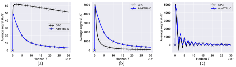
Figure 1: Average regret when $\mathbf{(a)}$: $\bm{\theta}_{t}\!=\!(1,1),\bm{w}_{t}\!=\!-(0.1,0.1)\forall t$; $\mathbf{(b)}$: $\bm{\theta}_{t}\!=\!(10,10),\bm{w}_{t}\!=\!-(1,1)\forall t$; $\mathbf{(c)}$: $\theta_{t}\!=\!(10,10)$ or $-(10,10)$ (Alternating every $1000$ steps), $\bm{w}_{t}\!=\!-(1,1)\forall t$.

6 Auxiliary Lemmas

Lemma 6.1.

The distance between parameters $M_{t-i-1}$ and $M_{t}$, with $i\leq t-1$, where each $M_{t}$ is updated using (8), with regularizers (9), can be bounded as $\|{M}_{t-i-1}-{M}_{t}\|\leq\sum_{\tau=t-i-1}^{t-1}\frac{\|G_{\tau}\|}{\sigma_{1:\tau}}$.

Proof 6.2.

First, note that $\|{M}_{t-i-1}-{M}_{t}\|\leq\sum_{\tau=t-i-1}^{t-1}\|{M}_{\tau}-{M}_{\tau+1}\|$. To bound each $\|{M}_{\tau}-{M}_{\tau+1}\|$, we leverage (McMahan, 2017, Lem. 7) which states that given a convex function $\phi_{1}(\cdot)$ with a minimizer $q_{1}\doteq\operatorname*{argmin}_{q}{\phi_{1}(q)}$ and a function $\phi_{2}(\cdot)\!=\phi_{1}(\cdot)\!+\psi(\cdot)$ that is a strongly convex w.r.t a norm $\|\cdot\|$ and has minimizer $q_{2}\doteq\operatorname*{argmin}_{q}{\phi_{2}(q)}$, then we can bound the two minimizers as $\|q_{1}\!-\!q_{2}\|\!\leq\|b\|_{*}$ for some (sub)gradient $b\in\partial\psi({q}_{1})$. Now, we invoke this result by setting:

$$q_{1}=M_{\tau},\ \ q_{2}={M}_{\tau+1},\quad\phi_{1}(M)=\sum_{s=1}^{\tau-1}\Big{(}c_{s}\big{(}\bm{x}_{s}(\pi),\bm{u}_{s}(\pi)\big{)}+r_{s}(M)\Big{)}+r_{\tau}(M),\quad\text{and}$$ (22)

$$\phi_{2}(M)=\sum_{s=1}^{\tau-1}\Big{(}c_{s}\big{(}\bm{x}_{s}(\pi),\bm{u}_{s}(\pi)\big{)}+r_{s}(M)\Big{)}+r_{\tau}(M)+\underbrace{c_{\tau}\big{(}\bm{x}_{\tau}(\pi),\bm{u}_{\tau}(\pi)\big{)}}_{\psi(M)}.$$ (23)

The function $\phi_{2}(M)$ is strongly-convex w.r.t. the norm $\|\cdot\|_{\tau}=\sqrt{\sigma_{1:\tau}}\|\cdot\|$, a property inherited due to containing the sum of all regularizers up to step $\tau$, i.e., $\sum_{s=1}^{\tau}r_{s}(M)$. And the dual norm of the gradient of the above-defined $\psi(M)$ function, at each step $s$, is upper-bounded by $\|G_{s}\|_{\tau,*}$.

Finally, it suffices to observe that: $(i)$ based on the definition of the update rule for variables $M$, and $(ii)$ the fact that $r_{t}(M),\forall t$ is a proximal regularizer thus $r_{t}(M_{t})=0,\forall t$, we indeed have that $M_{\tau}=\operatorname*{argmin}_{M\in\mathcal{M}}\phi_{1}(M)$ and $M_{\tau+1}=\operatorname*{argmin}_{M\in\mathcal{M}}\phi_{1}(M)+\psi(M)$. Now, applying (McMahan, 2017, Lem. 7) we obtain $\|{M}_{\tau}-{M}_{\tau+1}\|_{\tau}\leq\|G_{\tau}\|_{\tau,*}\rightarrow\|{M}_{\tau}-{M}_{\tau+1}\|\leq\frac{\|G_{\tau}\|}{\sigma_{1:\tau}}$.

Lemma 6.3.

Let $a_{0}\geq 0$, $\delta\in(0,1]$ and $f:[0,\infty]\mapsto[0,\infty)$ be a non-increasing function. Then:

$$\mathcal{S}\doteq\sum_{t=1}^{T}\sum_{i=0}^{t-1}(1-\delta)^{i}\sum_{\tau=t-i}^{t}a_{\tau}\ f(a_{0:\tau})\leq\frac{1}{\delta^{2}}\int_{a_{0}}^{a_{1:T}}{f(x)dx}$$ (24)

Proof 6.4.

Instead of summing over all $i<t$ for each $t\in[1,T]$, the sum $\mathcal{S}$ can be equivalently re-written by summing over all $t>i$ for each $i\in[0,T]$:

$$\mathcal{S}=\sum_{i=0}^{T}(1-\delta)^{i}\sum_{t=i+1}^{T}\sum_{\tau=t-i}^{t}a_{\tau}\ f(a_{0:\tau})$$ (25)

Now we bound $\mathcal{S}^{\prime}\doteq\sum_{t=i+1}^{T}\sum_{\tau=t-i}^{t}a_{\tau}\ f(a_{0:\tau})$. Let $s_{t}\doteq a_{0:t}$

$$\sum_{\tau=t-i}^{t}\!\!a_{\tau}\!\!\ f(a_{0:\tau})=\sum_{\tau=0}^{i}a_{t-\tau}f(s_{t-\tau})=\sum_{\tau=0}^{i}\int_{s_{t-\tau-1}}^{s_{t-\tau}}f(s_{t-\tau})dx\leq\sum_{\tau=0}^{i}\int_{s_{t-\tau-1}}^{s_{t-\tau}}f(x)dx.$$ (26)

$$\text{Hence, }\mathcal{S}^{\prime}\leq\sum_{\tau=0}^{i}\sum_{t=i+1}^{T}\int_{s_{t-\tau-1}}^{s_{t-\tau}}\!\!\!\!f(x)dx\leq\sum_{\tau=0}^{i}\int_{s_{i-\tau}}^{s_{T-\tau}}\!\!\!\!f(x)dx\leq\sum_{\tau=0}^{i}\int_{s_{0}}^{s_{T}}\!\!\!\!f(x)dx=(i\!+\!1)\!\!\int_{s_{0}}^{s_{T}}\!\!\!\!f(x)dx.$$ (27)

substituting the bound for $\mathcal{S}^{\prime}$ back in (25) we get:

$$\mathcal{S}\leq \sum_{i=0}^{T}(1-\delta)^{i}(i+1)\!\!\int_{s_{0}}^{s_{T}}\!\!\!\!f(x)dx\leq\frac{1}{\delta^{2}}\int_{s_{0}}^{s_{T}}\!\!\!\!f(x)dx.$$ (28)

Where we used that $\sum_{i=0}^{\infty}\!i(1\!-\!\delta)^{i}\!\leq\!\nicefrac{{1\!-\!\delta}}{{\delta^{2}}}$ and $\sum_{i=0}^{\infty}(1\!-\!\delta)^{i}\!\!\leq\!\nicefrac{{1}}{{\delta}}$.

References

- Agarwal et al. (2019a) Naman Agarwal, Brian Bullins, Elad Hazan, Sham Kakade, and Karan Singh. Online control with adversarial disturbances. In Proc. of ICML, 2019a.
- Agarwal et al. (2019b) Naman Agarwal, Elad Hazan, and Karan Singh. Logarithmic regret for online control. In Proc. of NeurIPS, 2019b.
- Anava et al. (2015) Oren Anava, Elad Hazan, and Shie Mannor. Online learning for adversaries with memory: Price of past mistakes. In Proc. of NeurIPS, 2015.
- Auer et al. (2002) Auer et al. Adaptive and self-confident on-line learning algorithms. Journal of Computer and System Sciences, 64(1):48–75, 2002. ISSN 0022-0000.
- Cesa-Bianchi et al. (2013) Nicolo Cesa-Bianchi, Ofer Dekel, and Ohad Shamir. Online learning with switching costs and other adaptive adversaries. In Proc. of NeurIPS, 2013.
- Cohen et al. (2018) Alon Cohen, Avinatan Hasidim, Tomer Koren, Nevena Lazic, Yishay Mansour, and Kunal Talwar. Online linear quadratic control. In Proc. of ICML, 2018.
- Duchi et al. (2011) John Duchi, Elad Hazan, and Yoram Singer. Adaptive subgradient methods for online learning and stochastic optimization. Journal of Machine Learning Research, 12(61):2121–2159, 2011.
- Foster and Simchowitz (2020) Dylan Foster and Max Simchowitz. Logarithmic regret for adversarial online control. In Proc. of ICML, 2020.
- Goel and Hassibi (2022) Gautam Goel and Babak Hassibi. Competitive control. IEEE Trans. Autom. Control, 2022. 10.1109/TAC.2022.3218769.
- Goel et al. (2023) Gautam Goel, Naman Agarwal, Karan Singh, and Elad Hazan. Best of both worlds in online control: Competitive ratio and policy regret. In Proc. of L4DC, 2023.
- Gofer (2014) Eyal Gofer. Higher-order regret bounds with switching costs. In Proc. of COLT, 2014.
- Gradu et al. (2020) Paula Gradu, John Hallman, and Elad Hazan. Non-stochastic control with bandit feedback. In Proc. of NeurIPS, 2020.
- Gradu et al. (2023) Paula Gradu, Elad Hazan, and Edgar Minasyan. Adaptive regret for control of time-varying dynamics. In Proc. of L4DC, 2023.
- Hazan and Singh (2022) Elad Hazan and Karan Singh. Introduction to online nonstochastic control. arXiv:2211.09619, 2022.
- Hazan et al. (2020) Elad Hazan, Sham Kakade, and Karan Singh. The nonstochastic control problem. In Proc. of ALT, 2020.
- Jin et al. (2023) Tiancheng Jin, Junyan Liu, Chloé Rouyer, William Chan, Chen-Yu We, and Haipeng Luo. No-regret online reinforcement learning with adversarial losses and transitions. arXiv:2305.17380, 2023.
- Lee et al. (2021) Russell Lee, Jessica Maghakian, Mohammad Hajiesmaili, Jian Li, Ramesh Sitaraman, and Zhenhua Liu. Online peak-aware energy scheduling with untrusted advice. ACM SIGENERGY Energy Informatics Review, 1(1):59–77, 2021.
- Li et al. (2021) Yingying Li, Subhro Das, and Na Li. Online optimal control with affine constraints. Proceedings of the AAAI Conference on Artificial Intelligence, 2021.
- Liu et al. (2023) Xin Liu, Zixian Yang, and Lei Ying. Online nonstochastic control with adversarial and static constraints. arXiv:2302.02426, 2023.
- McMahan (2017) H. Brendan McMahan. A Survey of Algorithms and Analysis for Adaptive Online Learning. J. Mach. Learn. Res., 18(1):3117–3166, 2017.
- Orabona (2023) Francesco Orabona. A Modern Introduction to Online Learning. arXiv:1912.13213, 2023.
- Shalev-Shwartz (2012) Shai Shalev-Shwartz. Online learning and online convex optimization. Foundations and Trends in Machine Learning, 4(2):107–194, 2012. ISSN 1935-8237. 10.1561/2200000018.
- Shi et al. (2020) Guanya Shi, Yiheng Lin, Soon-Jo Chung, Yisong Yue, and Adam Wierman. Online optimization with memory and competitive control. In Proc. of NeurIPS, 2020.
- Simchowitz (2020) Max Simchowitz. Making non-stochastic control (almost) as easy as stochastic. In Proc. of NeurIPS, 2020.
- Simchowitz et al. (2020) Max Simchowitz, Karan Singh, and Elad Hazan. Improper learning for non-stochastic control. In Proc. of COLT, 2020.
- Suo et al. (2021) Daniel Suo, Naman Agarwal, Wenhan Xia, Xinyi Chen, Udaya Ghai, Alexander Yu, Paula Gradu, Karan Singh, Cyril Zhang, Edgar Minasyan, et al. Machine learning for mechanical ventilation control. arXiv:2102.06779, 2021.
- Zhang et al. (2022) Zhiyu Zhang, Ashok Cutkosky, and Ioannis Paschalidis. Adversarial tracking control via strongly adaptive online learning with memory. In Proc. of AISTATS, 2022.
- Zhao et al. (2022) Peng Zhao, Yu-Xiang Wang, and Zhi-Hua Zhou. Non-stationary online learning with memory and non-stochastic control. In Proc. of AISTATS, 2022.