Learning unitaries with quantum statistical queries

Abstract

We propose several algorithms for learning unitary operators from quantum statistical queries (QSQs) with respect to their Choi-Jamiolkowski state. Quantum statistical queries capture the capabilities of a learner with limited quantum resources, which receives as input only noisy estimates of expected values of measurements. Our methods hinge on a novel technique for estimating the Fourier mass of a unitary on a subset of Pauli strings with a single quantum statistical query, generalizing a previous result for uniform quantum examples. Exploiting this insight, we show that the quantum Goldreich-Levin algorithm can be implemented with quantum statistical queries, whereas the prior version of the algorithm involves oracle access to the unitary and its inverse. Moreover, we prove that $\mathcal{O}(\log n)$-juntas and quantum Boolean functions with constant total influence are efficiently learnable in our model, and constant-depth circuits are learnable sample-efficiently with quantum statistical queries. On the other hand, all previous algorithms for these tasks require direct access to the Choi-Jamiolkowski state or oracle access to the unitary. In addition, our upper bounds imply that the actions of those classes of unitaries on locally scrambled ensembles can be efficiently learned. We also demonstrate that, despite these positive results, quantum statistical queries lead to an exponentially larger sample complexity for certain tasks, compared to separable measurements to the Choi-Jamiolkowski state. In particular, we show an exponential lower bound for learning a class of phase-oracle unitaries and a double exponential lower bound for testing the unitarity of channels, adapting to our setting previous arguments for quantum states. Finally, we propose a new definition of average-case surrogate models, showing a potential application of our results to hybrid quantum machine learning.

Learning the dynamic properties of quantum systems is a fundamental problem at the intersection of machine learning (ML) and quantum physics. In the most general case, this task can be achieved under the broad framework of quantum process tomography (QPT) [1]. However, QPT can be extremely resource-intensive, as learning the entire classical description of a unitary transformation requires exponentially many queries [2] in the worst case. This complexity can be significantly reduced if the unitary is not completely arbitrary, but instead it belongs to a specific class. For instance, this approach has been fruitfully adopted for quantum Boolean functions [3], quantum juntas [4, 5] and quantum circuits with bounded covering numbers [6]. On the other hand, the complexity of quantum process tomography could be drastically reduced if we restrict our attention only on local properties of the output state, as recently demonstrated in [7]. Another scenario of interest is the one of property testing, where the learner is not asked to retrieve the classical description of the target process, but solely to test whether is satisfies some specific property [8]. A further figure of merit in quantum process learning is the type of resources that the learner is allowed to use. For the special case of unitary transformations, the learner is usually given oracle access to the target unitary $U$ and its inverse $U^{\dagger}$, or, alternatively, to the corresponding Choi-Jamiolkowski state. In this paper we consider this latter approach and we ask the following question:

Which classes of unitaries are efficiently learnable with noisy single-copy measurements of the Choi-Jamiolkowski state?

This question is motivated by near-term implementations of quantum algorithms, which involve several sources of noise and severely limited entangling capacity [9]. To this end, we adopt the model of quantum statistical queries (QSQs), previously introduced in [10, 11] as an extension of the (classical) statistical query model [12]. In the QSQ model, we consider a learner without quantum memory that can only access noisy estimates of the expected values of chosen observables on an unknown initial state. Interestingly, several concept classes such as parities, juntas function, and DNF formulae are efficiently learnable in the QSQ model, whereas the classical statistical query model necessitates an exponentially larger number of samples. Despite these positive results, resorting to quantum statistical queries can be considerably limiting for some tasks. In particular, the authors of [11] have established an exponential gap between QSQ learning and learning with quantum examples in the presence of classification noise. Quantum statistical queries have also found practical applications in classical verification of quantum learning, as detailed in [13]. Furthermore, they have been employed in the analysis of quantum error mitigation models [14, 11] and quantum neural networks [15]. Alternative variations of quantum statistical queries have also been explored in [16, 17, 18]. Moreover, the connection between quantum statistical queries and quantum differential privacy was investigated in [10], and an equivalence between quantum statistical query learning and quantum local differential privacy [19] .

Our contributions.

In this paper we demonstrate that several classes of unitaries are efficiently learnable with quantum statistical queries with respect to their Choi state. In particular, we show our result for a natural distance over unitaries induced by the Choi-Jamiolkowski isomorphism and previously adopted in [8, 5]. We emphasize that this choice of distance allows to predict the action of the target unitary on a random input state sampled from a locally scrambled ensemble [20]. We now give an informal version of our upper bounds. When not explicitly stated, the tolerance of a quantum statistical query is at least polynomially small.

• Constant depth circuits are learnable with polynomially many quantum statistical queries (Theorem 3.2).

• Quantum $O(\log n)$-juntas are efficiently learnable with polynomially many quantum statistical queries (Theorem 3.3).

• Quantum Boolean functions with constant total influence are efficiently learnable with polynomially many quantum statistical queries (Theorem 3.5). In order to prove this result, we show that the quantum Goldreich-Levin algorithm can be implemented with quantum statistical queries (Theorem 3.4).

While these positive results show that a wide class of unitaries can be efficiently learned in our model, we also argue that resorting to quantum statistical queries leads to an exponentially larger sample complexity for certain tasks. In particular, we give the following lower bound.

• There is a class of phase oracle unitaries that requires exponentially many quantum statistical queries with polynomially small tolerance to be learnt below distance $0.005$ with high probability (Theorem 4.1);

• Estimating the unitarity of a quantum channel with error smaller than $0.24$ and polynomially small tolerance requires double-exponentially many quantum statistical queries (Theorem 4.2).

Moreover, prior results imply that both tasks can be efficiently performed with polynomially many copies of the associated Choi-Jamiolkowski state. In Section 3.3.1, we complement our theoretical findings with a numerical simulation the quantum Goldreich-Levin algorithm implemented with quantum statistical queries. Finally, in Section 5 we suggest a potential application of our results to hybrid quantum machine learning. Prior work [21, 22] showed that certain quantum learning models can be replaced by classical surrogates during the prediction phase. We argue that the learning algorithms provided in the present paper can also serve to this scope. To this end, we extend the definition of classical surrogates from the worst-case to the average-case.

Related work.

Our results generalize prior work in two ways. On the one hand, we show that several classes of unitaries are learnable in the QSQ model, while all previous results involved the access to stronger oracles. The adoption of a weaker oracle is particularly advantageous for near-term implementation, since the definition of QSQs accounts for the measurement noise. On the other hand, we demonstrate that prior QSQ algorithms for learning classical Boolean functions can be generalized to unitary learning. In particular, Chen et al. [4] showed that $k$-junta unitaries are learnable with $O(4^{k})$ copies of the Choi state, and Montanaro and Osborne [3] proposed the original version of the quantum Goldreich-Levin algorithm, requiring oracle access to the target unitary and its inverse.

Furthermore, Atıcı and Servedio [23] provided an algorithm for learning classical $k$-junta functions with $O(2^{k})$ uniform quantum examples, and Arunachalam et al. [10] demonstrated that several classes of quantum Boolean functions are learnable with quantum statistical queries with respect to uniform quantum examples. In particular, they showed that classical $k$-junta functions are learnable with $O(2^{k}+n)$ quantum statistical queries, and moreover that the (classical) Goldreich-Levin algorithm can be implemented in the QSQ model. In a subsequent work, Arunachalam et al. [11] showed that the output of constant-depth circuits is learnable with $\mathrm{poly}(n)$ quantum statistical queries and provided several hardness results for the QSQ model. Specifically, they showed an exponential lower bound for learning a class of classical Boolean functions, and a double exponential lower bound for testing the purity of a target state.

Open questions.

We distil several open questions concerning quantum statistical queries and process learning.

1. The main workhorse for QSQ learning classical Boolean functions is Fourier analysis. While Fourier analysis is usually cast under the uniform distribution, the $\mu$-biased Fourier analysis can be applied to every product distribution. In particular, $\mu$-biased Fourier sampling can be used to learn linear functions [24] and DNFs [25] under product distributions with quantum examples. Can we extend these results to the QSQ model?

2. Which classes of channels can be learned under quantum statistical queries?

3. What is the power of quantum statistical queries for testing properties of unitaries (and more broadly channels)? While we provided a double exponential lower bound for testing unitarity, quantum statistical queries might suffice for testing other relevant properties.

4. Following [16, 18], we can restrict our model to diagonal measurements. Which classes of channels are learnable under this restricted model?

1 Preliminaries

We start by introducing the mathematical notation and the background. For $n\geq 1$, we will write $[n]=\{1,2,\dots,n\}$. Given $T\subseteq[n]$, we will write $\overline{T}:=[n]\setminus T$. We will denote the $2^{n}\times 2^{n}$ identity matrix as $I_{n}$ and we may omit the index $n$ when is clear from the context. For a matrix $A$, we will denote as $A_{ij}$ the entry corresponding to the $i$-th row and the $j$-th column. We will use the indicator string $\mathbb{S}=(x_{1},x_{2},\dots,x_{k},*,*\dots,*)$ to denote the set of $n$-element strings whose first $k$ elements are $x_{1},x_{2},\dots,x_{k}$, i.e. $\mathcal{S}=\{(t_{1},t_{2},\dots,t_{n})|\;\forall i\in[k]:x_{i}=t_{i}\}$. Given a random variable $X$ sampled according to a distribution $\nu$, we will denote by $\mathbb{E}_{\nu}[X]$ its expected value and its variance by $\mathbb{V}_{\nu}[X]$, and omit the index $\nu$ when it’s clear from the context.

1.1 Quantum information theory

Let $\{\ket{0},\ket{1}\}$ be the canonical basis of $\mathbb{C}^{2}$, and $\mathcal{H}_{n}=(\mathbb{C}^{2})^{\otimes n}$ be the Hilbert space of $n$ qubits. We use the bra-ket notation, where we denote a vector $v\in(\mathbb{C}^{2})^{\otimes n}$ using the ket notation $\ket{v}$ and its adjoint using the bra notation $\bra{v}$. For $u,v\in\mathcal{H}_{n}$, we will denote by $\braket{u}{v}$ the standard Hermitian inner product $u^{\dagger}v$. A pure state is a normalized vector $\ket{v}$, i.e. $|\braket{v}{v}|=1$. Let $\mathcal{L}_{n}$ be the subset of linear operators on $\mathcal{H}_{n}$ and let $\mathcal{O}_{n}\subset\mathcal{L}_{n}$ be the subset of self-adjoint linear operators on $\mathcal{H}_{n}$. We represent the $2^{n}\times 2^{n}$ identity operator as $I_{n}$ and we omit the index $n$ when it is clear from the context. We denote by $\mathcal{O}^{T}_{n}\subset\mathcal{O}_{n}$ be the subset of traceless self-adjoint linear operators on $\mathcal{H}_{n}$, by $\mathcal{O}^{+}_{n}\subset\mathcal{O}_{n}$ the subset of the positive semidefinite linear operators on $\mathcal{H}_{n}$ and by $\mathcal{S}_{n}\subset\mathcal{O}^{+}_{n}$ the set of the quantum states of $\mathcal{H}_{n}$, i.e. $\mathcal{S}_{n}:=\{\rho\in\mathcal{L}_{n}:\rho\geq 0,\mathrm{Tr}[\rho]=1\}$. We denote by $\mathcal{U}_{n}$ the unitary group, that is the set linear operators $U\in\mathcal{L}_{n}$ satisfying $UU^{\dagger}=U^{\dagger}U=I$, and we denote by $\mathrm{Id}:\mathcal{L}_{n}\rightarrow\mathcal{L}_{n}$ the identity map. For any operators $A,B\in\mathcal{L}_{n}$, let $\braket{A,B}$, denote the normalized Hilbert-Schmidt inner product,

$$\braket{A,B}=\frac{1}{2^{n}}\mathrm{Tr}[A^{\dagger}B]=\frac{1}{2^{n}}\sum_{i,j\in\{0,1\}^{n}}A^{*}_{ij}B_{ij}.$$ (1)

We define the canonical maximally entangled state as $\ket{\Omega}=\frac{1}{\sqrt{2^{n}}}\sum_{i,j\in\{0,1\}^{n}}\ket{i,i}$. Moreover, the identity $\mathbb{I}$ and the flip operator $\mathbb{F}$ associated to a tensor product of two Hilbert spaces $\mathcal{H}_{n}^{\otimes 2}$ are defined as

$$\mathbb{I}:=\sum_{i,j\in\{0,1\}^{n}}|{i,j}\rangle\langle{i,j}|,\quad\quad\quad\mathbb{F}:=\sum_{i,j\in\{0,1\}^{n}}|{i,j}\rangle\langle{j,i}|.$$ (2)

Notably, they satisfy the following properties:

$$\mathbb{I}\left(\ket{\psi}\otimes\ket{\phi}\right)=\ket{\psi}\otimes\ket{\phi},\quad\quad\mathbb{F}\left(\ket{\psi}\otimes\ket{\phi}\right)=\ket{\phi}\otimes\ket{\psi},$$ (3)

for all $\ket{\psi},\ket{\phi}\in\mathcal{H}_{n}$. We denote by $\mathcal{P}_{n}:=\{I,X,Y,Z\}^{\otimes n}$ the Pauli basis. Elements of the Pauli basis are Hermitian, unitary, trace-less, they square to the identity and they are orthonormal to each other with respect the normalized Hilbert-Schmidt inner product. The Pauli basis forms an orthonormal basis for the set of linear operators $\mathcal{L}_{n}$. We also define the single-qubit stabilizers states as the eigenstates of single-qubit Pauli operators, i.e. $\mathsf{stab}:=\{|0\rangle,|1\rangle,|+\rangle,|-\rangle,|+y\rangle,|-y\rangle\}$.

1.2 Ensembles of states and unitaries

We start by providing some rudimentary notions about the Haar measure $\mu_{n}$, which can be thought as the uniform distribution over the unitary group $\mathcal{U}_{n}$. For a comprehensive introduction to the Haar measure and its properties, we refer to [26]. The Haar measure on the unitary group $\mathcal{U}_{n}$ is the unique probability measure $\mu_{n}$ that is both left and right invariant over the set $\mathcal{U}_{n}$, i.e., for all integrable functions $f$ and for all $V\in\mathcal{U}_{n}$, we have:

$$\int_{\mathcal{U}_{n}}f(U)d\mu_{n}(U)=\int_{\mathcal{U}_{n}}f(UV)d\mu_{n}(U)=\int_{\mathcal{U}_{n}}f(VU)d\mu_{n}(U).$$ (4)

Given a state $\ket{\phi}$, we denote the $k$-th moment of a Haar random state as

$$\mathbb{E}_{\ket{\psi}\sim\mu_{n}}\left[\ket{\psi}\bra{\psi}^{\otimes k}\right]:=\mathbb{E}_{U\sim\mu_{n}}\left[U^{\otimes k}\ket{\phi}\bra{\phi}^{\otimes k}U^{{\dagger}\otimes k}\right].$$ (5)

Note that the right invariance of the Haar measure implies that the definition of $\mathbb{E}_{\ket{\psi}\sim\mu_{n}}\left[\ket{\psi}\bra{\psi}^{\otimes k}\right]$ does not depend on the choice of $\ket{\phi}$. In many scenarios, random unitaries and states are sampled from distributions that match only the low-order moments of the Haar measure. This leads to the definition of $t$-designs, for integers $t\geq 1$. Let $\nu$ be a probability distribution over the set of quantum states $\mathcal{S}_{n}$. The distribution $\nu$ is said to be a state $t$-design if

$$\mathbb{E}_{\ket{\psi}\sim\nu}\left[|{\psi}\rangle\langle{\psi}|^{\otimes t}\right]=\mathbb{E}_{\ket{\psi}\sim\mu_{n}}\left[|{\psi}\rangle\langle{\psi}|^{\otimes t}\right].$$ (6)

Along with $t$-designs and Haar random ensembles, another important family of states (and unitaries) is the one of locally scrambled ensembles, introduced in [20]. An ensemble of $n$-qubit unitaries is called locally scrambled if it is invariant under pre-processing by tensor products of arbitrary local unitaries. That is, a unitary ensemble $\mathcal{U}_{\mathrm{LS}}$ is locally scrambled if for $U\sim\mathcal{U}_{\mathrm{LS}}$ and for any fixed $U_{1},\dots,U_{n}\in\mathcal{U}_{1}$ also $U(\bigotimes^{n}_{i=1}U_{i})\sim\mathcal{U}_{\mathrm{LS}}$. Accordingly, an ensemble $\mathcal{S}_{\mathrm{LS}}$ of $n$-qubit quantum states is locally scrambled if it is of the form $\mathcal{S}_{\mathrm{LS}}=\mathcal{U}_{\mathrm{LS}}\ket{0^{n}}$ for some locally scrambled unitary ensemble $\mathcal{U}_{\mathrm{LS}}$. Notable examples of locally scrambled ensembles are the products of random single-qubit stabilizer states and the products of Haar random $k$-qubit states, which, in particular, include Haar random $n$-qubit states the products of Haar random single-qubit states. We emphasize that the above families include both product states and highly entangled states.

1.3 The Choi-Jamiolkowski isomorphism

Furthermore, we can represent a unitary $U\in\mathcal{U}_{n}$ with its dual pure state, known as Choi-Jamiolkowski state, or simply Choi state [27, 28]. The Choi state $\ket{v(U)}$ can be prepared by first creating the maximally entangled state on $2n$ qubits, which we denoted by $\ket{\Omega}$, and then applying $U$ on half of the maximally entangled state. This is equivalent to preparing $n$ Einstein–Podolsky–Rosen (EPR) pairs $\frac{1}{\sqrt{2}}(\ket{00}+\ket{11})$ (which altogether forms $2n$ qubits) and applying the unitary $U$ to the $n$ qubits coming from the second half of each of the EPR pairs. We have

$$\ket{v(U)}=(I_{n}\otimes U)\ket{\Omega}=\frac{1}{\sqrt{2^{n}}}\sum_{i\in\{0,1\}^{n}}\ket{i}\otimes U\ket{i}=\frac{1}{\sqrt{2^{n}}}\sum_{i\in\{0,1\}^{n}}U_{ji}\ket{i,j}$$ (7)

This definition can be naturally extended to a general quantum channel $\mathcal{N}$:

$$\mathcal{J}(\mathcal{N})=\mathrm{Id}\otimes\mathcal{N}(|{\Omega}\rangle\langle{\Omega}|)=\frac{1}{2^{n}}\sum_{i,j\in\{0,1\}^{n}}|{i}\rangle\langle{j}|\otimes\mathcal{N}(|{i}\rangle\langle{j}|).$$ (8)

Clearly, $\mathcal{J}(U(\cdot)U^{\dagger})=|{v(U)}\rangle\langle{v(U)}|$. Furthermore, we recall that each EPR pair can be prepared by a circuit of depth 2:

$$\frac{1}{\sqrt{2}}(\ket{00}+\ket{11})=\mathsf{CNOT}(H\otimes I)\ket{00}.$$ (9)

Then that the $n$ EPR pairs may be prepared in parallel with a constant depth circuit. The Choi states of Pauli strings is of particular interest:

$$\ket{v(I)}=\frac{1}{\sqrt{2}}(\ket{00}+\ket{11}),\;\ket{v(X)}=\frac{1}{\sqrt{2}}(\ket{01}+\ket{10})$$ (10)

$$i\ket{v(Y)}=\frac{1}{\sqrt{2}}(\ket{01}-\ket{10}),\;\ket{v(Z)}=\frac{1}{\sqrt{2}}(\ket{00}-\ket{11}).$$ (11)

We note that the Choi states of the Pauli basis are proportional to the Bell basis. This readily implies that the set $\left\{\ket{v(I)},\ket{v(X)},\ket{v(Y)},\ket{v(Z)}\right\}^{\otimes n}$ forms an orthonormal basis for $2n$-qubit pure states with respect to the standard Hermitian inner product, i.e. $\forall P,Q\in\mathcal{P}_{n}:|\braket{v(P)}{v(Q)}|=\delta_{P,Q}$, where $\delta_{P,Q}$ is the Kronecker’s delta function.

1.4 Distance between unitaries and expected risk

The Choi-Jamiolkowski isomorphism induces a distance over unitaries, introduced in [29] and recently extended to general quantum channels in [5]. In particular, we define

$${D}(U,V):=\||{v(U)}\rangle\langle{v(U)}|-|{v(V)}\rangle\langle{v(V)}|\|_{\mathrm{tr}}=\sqrt{1-|\braket{v(U)}{v(V)}|^{2}}.$$ (12)

We remark that closely related distances have also appeared in other works. In particular, the pseudo-distance $\mathrm{dist}(U,V)$ of [30, 4] and $D(U,V)$ are within a constant factor $\sqrt{2}$, as also shown in ([5], Lemma 14). We now state a useful result relating $D(\cdot,\cdot)$ to the action of unitaries on random states. To this end, we recall the definition of expected risk introduced in [20]. Let $\nu$ a distribution over pure states. We have,

$$\mathcal{R}_{\nu}(U,V):=\mathbb{E}_{\ket{\psi}\sim\nu}\left[\left\|U|{\psi}\rangle\langle{\psi}|U^{\dagger}-V|{\psi}\rangle\langle{\psi}|V^{\dagger}\right\|_{\mathrm{tr}}^{2}\right],$$ (13)

We now rephrase a result of [8] according to our notation.

Lemma 1.1 ([8], Proposition 21).

Let $\mu_{n}$ be the Haar measure over $n$-qubit states. For unitary operators $U,V\in\mathcal{U}_{n}$, it holds that

$$\mathcal{R}_{\mu_{n}}(U,V)=\frac{2^{n}}{2^{n}+1}D(U,V)^{2}$$ (14)

Therefore, ${D}(U,V)$ is an “average-case” measure of the distance between quantum channels, and it is closely related to task of learning the action of a unitary on a Haar-random state. Moreover, the following result swiftly extends this guarantee to all locally scrambled ensembles of states.

Lemma 1.2 ([20], Lemma 1, Lemma B.4).

Let $\nu$ a locally scrambled ensemble of states. We have,

$$\frac{1}{2}\mathcal{R}_{\mu_{n}}(U,V)\leq\frac{2^{n}}{2^{n}+1}\mathcal{R}_{\nu}(U,V)\leq\mathcal{R}_{\mu_{n}}(U,V).$$ (15)

1.5 Fourier analysis on the unitary group

Let $U\in\mathcal{U}_{n}$ a unitary and consider the Pauli expansion $U=\sum_{P\in\mathcal{P}_{n}}\widehat{U}_{P}P$. We observe that the corresponding Choi state $\ket{v(U)}$ admits an analogous expansion with the same coefficients:

$$\ket{v(U)}=\left(I_{n}\otimes\sum_{P\in\mathcal{P}_{n}}\widehat{U}_{P}P\right)\left({\frac{1}{\sqrt{2^{n}}}}\sum_{i\in\{0,1\}^{n}}\ket{i,i}\right)=\sum_{P\in\mathcal{P}_{n}}\widehat{U}_{P}\ket{v(P)}.$$ (16)

We now recall the notion of influence of qubits on linear operators, introduced in [3] in the context of Hermitian operators and further developed in [4, 31]. The related influence of variables is widely used in the analysis of Boolean functions [32]. We define the quantum analogue of the bit-flip map as superoperator on $\mathcal{L}_{n}$:

$$d_{j}:=I^{\otimes(j-1)}\otimes\left(I-\frac{1}{2}\mathrm{Tr}\right)\otimes I^{\otimes(n-j)}.$$ (17)

Then for $P=\bigotimes_{i=1}^{n}P_{i}\in\mathcal{P}_{n}$, we have

$$d_{j}P=\begin{cases}P&\;\;\text{ if $P_{j}\neq I,$}\\ 0&\;\;\text{ if $P_{j}=I.$}\end{cases}$$ (18)

For a linear operator $A\in\mathcal{L}_{n},A=\sum_{P\in\mathcal{P}_{n}}\widehat{A}_{P}P$, we have

$$d_{j}A=\sum_{P:P_{j}\neq I}\widehat{A}_{P}P.$$ (19)

For $p\geq 1$, we denote by $\operatorname{Inf}_{j}^{p}(A):=\|d_{j}A\|_{p}^{p}$ the $L^{p}$-influence of $j$ on the operator $A$. For $S\in[n]$, we denote by $\operatorname{Inf}^{p}(A):=\sum_{j=1}^{n}\operatorname{Inf}^{p}_{j}(A)$ the associated total $L^{p}$-influence. We will often omit the index $p$ when $p=2$. Following [4], we also define the influence of a subset of qubits $S\in[n]$ as

$$\operatorname{Inf}_{S}(A)=\sum_{\begin{subarray}{c}P\in\mathcal{P}_{n}:\\ \mathrm{supp}(P)\cap S\neq\emptyset\end{subarray}}|\widehat{A}_{P}|^{2}.$$ (20)

We observe that $\operatorname{Inf}_{j}(A)=\operatorname{Inf}_{\{j\}}(A)=\sum_{\begin{subarray}{c}P\in\mathcal{P}_{n}:P_{j}\neq I\end{subarray}}|\widehat{A}_{P}|^{2}$, as expected. Intuitively, the influence of a unitary $U$ on a subset of qubits is a quantitative measure of the action of $U$ on such subset.

2 The model

We first give the definition of the QSQ oracle. For a state $\rho\in\mathcal{S}_{n}$, the $\mathsf{QStat}_{\rho}$ oracle receives as input an observable $O\in\mathcal{L}_{n},\|O\|\leq 1$ and a tolerance parameter $\tau\geq 0$, and returns a $\tau$-estimate of $\mathrm{Tr}[O\rho]$, i.e.

$$\mathsf{QStat}_{\rho}:(O,\tau)\mapsto\mathrm{Tr}[\rho O]\pm\tau.$$ (21)

A typical choice of the target state is the uniform quantum example $\ket{\psi_{f}}:=\sum_{x\in\{0,1\}^{n}}\frac{1}{\sqrt{2^{n}}}\ket{x,f(x)}$, for a suitable Boolean function $f:\{0,1\}^{n}\rightarrow\{0,1\}$, which was first introduced in [33] and widely employed in previous works on quantum statistical query learning [10, 11]. In this case, we will shorten the notation to $\mathsf{QStat}_{f}=\mathsf{QStat}_{|{\psi_{f}}\rangle\langle{\psi_{f}}|}$. To adapt their framework to our goal of learning unitaries, we need to devise an alternative input state. A natural choice is the Choi-Jamiolkowki state, which found many applications in prior work about unitary learning [4], and more broadly process learning [34], motivating its adoption in the context of quantum statistical query. For brevity, we will write $\mathsf{QStat}_{U}$ instead of $\mathsf{QStat}_{|{v(U)}\rangle\langle{v(U)}|}$. We now detail the mutual relationship between the oracle $\mathsf{QStat}_{U}$ and the previous oracles defined in terms of quantum examples. To this end, we consider two unitaries implementing $f$, notably the bit-flip oracle $U_{f}$ and the phase oracle $V_{f}$. We have,

$$\forall x\in\{0,1\}^{n},y\in\{0,1\}:U_{f}\ket{x,y}=\ket{x,y\oplus f(x)},$$ (22)

$$\forall x\in\{0,1\}^{n}:V_{f}\ket{x}=(-1)^{f(x)}\ket{x}$$ (23)

In particular we note that $\ket{\psi_{f}}=\frac{1}{\sqrt{2^{n}}}U_{f}\sum_{x\in\{0,1\}^{n}}\ket{x,0}$. We show that $\mathsf{QStat}_{f}$ can be simulated by $\mathsf{QStat}_{U_{f}}$ and conversely $\mathsf{QStat}_{V_{f}}$ can be simulated by $\mathsf{QStat}_{f}$. The first result shows that our framework generalizes the previous one based on quantum examples, while the second one allows us to transfer lower bounds from classical Boolean functions to unitaries, as formalized in Theorem 4.1.

Lemma 2.1 (Relations between QSQ oracles).

Let $f:\{0,1\}^{n}\rightarrow\{0,1\}$ a Boolean function and consider the bit-flip oracle $U_{f}$ and the phase oracle $V_{f}$. Then for every observable $A\in\mathcal{L}_{n+1}$, there exists an observable $A^{\prime}\in\mathcal{L}_{2n+2}$ such that

$$\braket{\psi_{f}}{A}{\psi_{f}}=\braket{v(U_{f})}{A^{\prime}}{v(U_{f})}.$$ (24)

and, similarly, for every observable $B\in\mathcal{L}_{2n}$, there exists an observable $B^{\prime}\in\mathcal{L}_{n+1}$ such that

$$\braket{v(V_{f})}{B}{v(V_{f})}=\braket{\psi_{f}}{B^{\prime}}{\psi_{f}}.$$ (25)

Proof.

The first result follows by selecting $A^{\prime}=I_{n}\otimes|{0}\rangle\langle{0}|\otimes A$. As for the second result, we can write the following expansion $B=\sum_{P,Q\in\mathcal{P}_{n}}c_{P,Q}|{v(P)}\rangle\langle{v(Q)}|$. From ([3], Proposition 9), we know that $\ket{v(V_{f})}=\sum_{x\in\{0,1\}^{n}}\widehat{f(x)}\ket{v(Z^{x})}$, where we denoted $Z^{x}:=\bigotimes_{i\in[n]}Z^{x_{i}}$, with $Z^{0}=I$ and $Z^{1}=Z$. Hence

$$\braket{v(U_{f})}{B}{v(U_{f})}=\sum_{x\in\{0,1\}^{n}}c_{Z^{x},Z^{x}}^{2}\widehat{f(x)}^{2}.$$ (26)

Now, consider the observable $T=\sum_{x\in\{0,1\}^{n}}c_{Z^{x},Z^{x}}|{x}\rangle\langle{x}|\in\mathcal{L}_{n}$ and define

$$B^{\prime}=H^{\otimes(n+1)}(I_{n}\otimes|{1}\rangle\langle{1}|)\cdot T\cdot(I_{n}\otimes|{1}\rangle\langle{1}|)H^{\otimes(n+1)},$$ (27)

which is equivalent to perform the Fourier transform on $\ket{\psi_{f}}$, post-selecting on the last qubit being 1 and finally applying $T$ on $n$ qubits. The Fourier transform and the projection on $|{1}\rangle\langle{1}|$ give rise to

$$\ket{\widehat{\psi}_{f}}=\sum_{x\in\{0,1\}^{n}}\widehat{f(x)}\ket{x}.$$ (28)

Then the desired result follows by noting that

$$\braket{\psi_{f}}{B^{\prime}}{\psi_{f}}=\braket{\widehat{\psi}_{f}}{T}{\widehat{\psi}_{f}}=\sum_{x\in\{0,1\}^{n}}c_{Z^{x},Z^{x}}^{2}\widehat{f(x)}^{2}.$$ (29)

∎

We argue that this choice of the oracle is particularly suitable for learning the unitary evolution of states sampled from locally scrambled ensembles. This comes as a direct consequence of Lemmas 1.1 and 1.2, that together imply the following proposition.

Lemma 2.2.

For quantum unitaries $U,V\in\mathcal{U}_{n}$ and $\nu\in\mathcal{S}_{LS}$ a locally scrambled ensemble of states, it holds that

$$\frac{1}{2}D(U,V)^{2}\leq\mathcal{R}_{\nu}(U,V)\leq D(U,V)^{2},$$ (30)

where $D(U,V)^{2}=1-|\braket{v(U)}{v(V)}|^{2}$.

We also introduce the following notion of learnability of classes of unitaries with quantum statistical queries.

Definition 2.1 (Unitary learning with QSQs).

Let $\varepsilon\in[0,1]$, $\mathcal{C}\subseteq\mathcal{U}_{n}$ a class of unitaries and $\nu$ an ensemble of $n$-qubit states. We say that $\mathcal{C}$ is efficiently $\varepsilon$-learnable with quantum statistical queries with respect to $\nu$ if, for all $U\in\mathcal{C}$, there exists an algorithm $\mathcal{A}$ that runs in time $\mathrm{poly}(n)$, performs $\mathrm{poly}(n)$ queries to the oracle $\mathsf{QStat}_{U}$ with tolerance at least $1/\mathrm{poly}(n)$ and outputs a unitary $V\in\mathcal{U}_{n}$ such that

$$\mathcal{R}_{\nu}(U,V)\leq\varepsilon.$$ (31)

We emphasize that all the algorithms proposed in this work are proper learners, in the sense that they output a unitary $V\in\mathcal{C}$. Moreover, they are classical randomized algorithms, as they use no other quantum resource apart from the query access to $\mathsf{QStat}_{U}$. The QSQ model is considerably more restrictive than the oracle access model, where a learner has the freedom to implement the unitary $U$ and its inverse $U^{\dagger}$ on an arbitrary input state. Then, every algorithm implementable with QSQs can be also implemented with oracle access, but the converse it is not true in general. In particular, we demonstrate in Theorem 4.1 that there is a class of unitaries that is efficiently learnable with direct access to the Choi state, but requires exponentially many quantum statistical queries.

3 Learning classes of unitaries with quantum statistical queries

Our results are based on the following technical lemma, which extends ([10], Lemma 4.1) to unitary operators. In particular, this lemma allows us to estimate the influence of subset of qubits defined in Eq. 20.

Lemma 3.1 (Learning the influence of a subset with a single QSQ).

Let $A\in\mathcal{U}_{n}$ be a unitary operator and $\mathsf{QStat}_{A}$ be the quantum statistical query oracle associated to the Choi state $\ket{v(A)}$. There is a procedure that on input a subset of Pauli strings $T\subseteq\mathcal{P}_{n}$, outputs $\tau$-estimate of $\sum_{P\in T}|\widehat{A}_{P}|^{2}$ using one query to $\mathsf{QStat}_{A}$ with tolerance $\tau$.

Proof.

Let $M=\sum_{P\in T}\ket{v(P)}\bra{v(P)}$. We note that

$$\bra{v(A)}M\ket{v(A)}= \left(\sum_{P\in\mathcal{P}_{n}}\widehat{A}^{*}_{P}\bra{v(P)}\right)\left(\sum_{Q\in T}\ket{v(Q)}\bra{v(Q)}\sum_{P\in\mathcal{P}_{n}}\widehat{A}_{P}\ket{v(P)}\right)$$ (32)

$$= \left(\sum_{P\in\mathcal{P}_{n}}\widehat{A}^{*}_{P}\bra{v(P)}\right)\left(\sum_{{Q}\in T}\widehat{A}_{Q}\ket{v(Q)}\right)=\sum_{P\in T}|\widehat{A}_{P}|^{2}.$$ (33)

Thus a single query to $\textsf{Qstat}_{A}$ with input $(M,\tau)$ yields the desired outcome. ∎

Remark 3.1 (Computational efficiency).

We observe that the circuit implementing the measurement $M=\sum_{P\in T}\ket{v(P)}\bra{v(P)}$ can have exponential depth in the worst case. However, in some cases, even if the set $T$ has exponential size, we can implement $M$ with a $\mathrm{poly}(n)$ circuit. For instance, the influence of the $j$-th qubit $\operatorname{Inf}_{j}(A)$ can be expressed as

$$\operatorname{Inf}_{j}(A)=\sum_{\begin{subarray}{c}P\in\mathcal{P}_{n}:\\ P_{j}\neq I\end{subarray}}|\widehat{A}_{P}|^{2}=1-\sum_{\begin{subarray}{c}P\in\mathcal{P}_{n}:\\ P_{j}=I\end{subarray}}|\widehat{A}_{P}|^{2}.$$ (34)

Thus it suffices to estimate the expected value of $\ket{v(I)}_{j}\bra{v(I)}_{j}\otimes I_{n-1}$. More generally, we can consider the indicator string $\mathbb{S}=(x_{1},x_{2},\dots,x_{k},*,*\dots,*)$ to denote the set of $n$-bit strings whose first $k$ elements are $x_{1},x_{2},\dots,x_{k}$, i.e. $\mathbb{S}=\{(t_{1},t_{2},\dots,t_{n})\in\{0,1,2,3\}^{n}|\;\forall i\in[k]:x_{i}=t_{i}\}$. Then we have,

$$\sum_{P\in\mathbb{S}}\ket{v(P)}\bra{v(P)}=\ket{v(\sigma_{x_{1}}\otimes\sigma_{x_{2}}\otimes\dots\otimes\sigma_{x_{k}})}\bra{v(\sigma_{x_{1}}\otimes\sigma_{x_{2}}\otimes\dots\otimes\sigma_{x_{k}})}\otimes I_{n-k},$$ (35)

which again can be implemented by a $\mathrm{poly}(n)$ circuit.

We will also need a further technical tool, which is an implementation of state tomography with quantum statistical queries, also previously exploited in [11] for learning the output of shallow circuits. Here we propose a refined argument for the special case of pure states. Since the complexity is exponential in the number of qubits, this primitive can be used to efficiently estimate the reduced states of subsets of logarithmic size.

Lemma 3.2 (State tomography).

Let $\rho\in\mathcal{S}_{n}$. There exists an algorithm that performs $4^{n}$ queries to the oracle $\mathsf{QStat}_{\rho}$ with tolerance at least $\varepsilon\cdot 4^{-n}$ and returns a state $\widehat{\rho}$ such that

$$\|\rho-\widehat{\rho}\|_{2}\leq\varepsilon.$$ (36)

Moreover, if $\rho=|{\psi}\rangle\langle{\psi}|$ is a pure state, there exists an algorithm that performs $4^{n}$ queries to the oracle $\mathsf{QStat}_{\rho}$ with tolerance at least $\varepsilon\cdot 2^{-n/2}$ and returns a pure state $\ket{\widehat{\psi}}$ such that

$$\|\rho-|{\widehat{\psi}}\rangle\langle{\widehat{\psi}}|\|_{\mathrm{tr}}\leq\varepsilon.$$ (37)

Proof.

We perform a state tomography by querying all $4^{n}-1$ non-identity Pauli strings with tolerance $\tau=\varepsilon\cdot 4^{-n}$. For all $P\in\mathcal{P}_{n}$, denote the obtained outcome by

$$o_{P}=\mathrm{Tr}[P\rho]\pm\tau$$

and set $x_{P}=\min\{o_{P},1\}$. Denote the estimated state by

$$\widehat{\rho}:=\frac{1}{2^{n}}\left(I+\sum_{\begin{subarray}{c}P\in\mathcal{P}_{n}\setminus I\end{subarray}}x_{P}P\right).$$ (38)

This allows to upper bound the distance between the partial state $\rho$ and its estimate $\widehat{\rho}$.

$$\|\rho-\widehat{\rho}\|_{2}^{2}= \mathrm{Tr}\left[(\rho-\widehat{\rho})^{2}\right]=\frac{1}{4^{n}}\mathrm{Tr}\left[\left(\sum_{P\in\mathcal{P}_{n}\setminus I}(\mathrm{Tr}[P\rho]-x_{P})P\right)^{2}\right]$$ (39)

$$= \frac{1}{2^{n}}\sum_{P\in\mathcal{P}_{n}\setminus I}(\mathrm{Tr}[P\rho]-x_{P})^{2}\leq 2^{n}\tau^{2},$$ (40)

where we used the inequality $(x+y)^{2}\leq 2(x^{2}+y^{2})$. Then picking $\tau=\varepsilon/\sqrt{2^{n}}$ gives the desired result. We now delve into the case where the input state is pure. Thanks to ([35], Theorem 1), and since $\rho=|{\psi}\rangle\langle{\psi}|$ has rank 1, we obtain the following bound for the 1-distance:

$$\|\rho-\widehat{\rho}\|_{1}\leq\sqrt{\frac{2^{n}}{2^{n}+1}}\|\rho-\widehat{\rho}\|_{2}\leq\varepsilon.$$ (41)

We now consider the dominant eigenstate of $\widehat{\rho}$, denoted by $\ket{\widehat{\psi}}$, which can be computed in $\mathrm{poly}(2^{n})$ time. By ([36], Proposition 2) we know that $|{\widehat{\psi}}\rangle\langle{\widehat{\psi}}|$ is the unique closest pure state to $\widehat{\rho}$. Since $\rho$ is also a pure state, this immediately implies

$$\left\||{\widehat{\psi}}\rangle\langle{\widehat{\psi}}|-{\rho}\right\|_{\mathrm{tr}}\leq \left\||{\widehat{\psi}}\rangle\langle{\widehat{\psi}}|-{\widehat{\rho}}\right\|_{\mathrm{tr}}+\|\rho-\widehat{\rho}\|_{\mathrm{tr}}$$ (42)

$$\leq 2\|\rho-\widehat{\rho}\|_{\mathrm{tr}}\leq\varepsilon,$$ (43)

∎

3.1 Appetizer: learning constant-depth circuits

As a first application of the tools introduced before, we show that very shallow circuits are learnable sample-efficiently with QSQs according to a locally scrambled distribution. We will rely on the following recent result of [37], which essentially shows that “learning marginal suffices”, i.e. learning the $k$-reduced density matrices of a state produced by a shallow circuit allows to perform a state tomography.

Theorem 3.1 (Adapted from [37], Theorem 4.3).

Let $\psi=|{\psi}\rangle\langle{\psi}|$ a state produced by a circuit of depth at most $D$. For any state $\rho$, one of the following conditions must be satisfied: either $\|\rho-\psi\|_{\mathrm{tr}}<\varepsilon$; or $\|\rho_{s}-\psi_{s}\|_{\mathrm{tr}}>{\varepsilon^{2}}/{n}$ for some $s\subseteq\{0,1,\dots,n-1\}$ with $|s|=2^{D}$.

An application of this result was also given in [11], where the authors showed that the class of $n$-qubit trivial states is learnable with $\mathrm{poly}(n)$ quantum statistical queries. We now extend their result from states to unitaries.

Theorem 3.2 (Learning constant-depth circuits via QSQs).

Let $\mathcal{C}$ the class of $\mathcal{O}(1)$-depth circuits. Then for all $U\in\mathcal{C}$, there exists an algorithm that makes $\mathrm{poly}(n)$ queries to $\mathsf{QStat}_{U}$ with tolerance at least $\frac{\varepsilon^{2}}{4n}\cdot 2^{-D/2}$ and returns a unitary $W\in\mathcal{U}_{n}$ such that

$$D(U,W)\leq\varepsilon.$$ (44)

Proof.

Let $D$ be the depth of the circuit. First, we consider the Choi state $\ket{v(U)}=I\otimes U\ket{\Omega}$ and recall that $\ket{\Omega}$ can be produced with a circuit of depth 2 over $2n$ qubits. Then we have $\ket{v(U)}=V\ket{0^{2n}}$ for a suitable unitary $V\in\mathcal{U}_{2n}$ implemented by a circuit of depth $D+2$. Let $k=2^{D+2}$. Then it suffices to learn all the $k$-local reduced density matrices of the states $\ket{v(U)}$. There are $\binom{2n}{k}=\mathcal{O}\left(n^{2^{D}}\right)$ of them and each of them is learnable in trace distance with accuracy $\frac{\varepsilon^{2}}{2n}$ by performing $4^{D+2}$ quantum statistical queries with tolerance $\frac{\varepsilon^{2}}{4n}\cdot 2^{-D/2}$ by means of Lemma 3.2. We can thus determine thanks to Theorem 3.1 a state $\ket{v(W)}$ such that $\||{v(W)}\rangle\langle{v(W)}|-|{v(U)}\rangle\langle{v(U)}|\|_{\mathrm{tr}}\leq\varepsilon$. This immediately implies Eq. 44 by Lemma 2.2. ∎

3.2 Learning quantum juntas

A unitary $U\in\mathcal{U}_{n}$ is a quantum $k$-junta if there exists $S\subseteq[n]$ with $|S|=k$ such that

$$U=V_{S}\otimes I_{\overline{S}}$$

for some $V_{S}\in\mathcal{U}_{k}$. For a Pauli string $P=\bigotimes_{i\in[n]}P_{i}\in\mathcal{P}_{n}$, we denote the reduced string as $P_{S}=\bigotimes_{i\in S}P_{i}\in\mathcal{P}_{k}$. We now consider the Pauli expansions $U=\sum_{P\in\mathcal{P}_{n}}\widehat{U}_{P}P$ and $V_{S}=\sum_{P_{S}\in\mathcal{P}_{k}}\widehat{V}_{P_{S}}P_{S}$. Their coefficients satisfy the following relation.

$$\widehat{U}_{P}=\frac{1}{2^{n}}\mathrm{Tr}[UP]=\frac{1}{2^{n}}\mathrm{Tr}[V_{S}P_{S}]\mathrm{Tr}[P_{\overline{S}}I_{\overline{S}}]=\begin{cases}\widehat{V}_{P_{S}}&\text{ if $\mathrm{supp}(P)\in S$,}\\ 0&\text{ else. }\end{cases}$$

As for the Choi state, we have

$$\ket{v(U)}=\sum_{P\in\mathcal{P}_{n}}\widehat{U}_{P}\ket{v(P)}=\sum_{\mathrm{supp}(P)\in S}\widehat{V}_{P_{S}}\ket{v(P_{S}\otimes I_{\overline{S}})}=\ket{v(V_{S})}\ket{v(I_{\overline{S}})}.$$

We will now show that quantum $k$-juntas are efficiently learnable in our model. Our proof combines the techniques used in [4] for learning quantum $k$-juntas from oracle access and the ones used in [10] for learning (classical) $k$-juntas with quantum statistical queries. Note that the algorithm given in ([4], Theorem 28) has query complexity independent of $n$. Crucially, their algorithm involves a Pauli sampling as a subroutine to estimate the support of the Pauli strings with non-zero Fourier coefficients. We replaced this procedure by estimating the influences of each qubit by means of Lemma 3.1, introducing an additional factor $n$ in the query complexity.

Algorithm 1 Learning quantum $k$-juntas with statistical queries

for $i=1$ to $n$ do

     Estimate $\operatorname{Inf}^{2}_{i}(U)$ with a quantum statistical query with accuracy $\varepsilon^{2}/(20k)$ and store the result in the variable $\alpha_{i}$.

end for

Define the subset $T=\left\{i\in[n]:\alpha_{i}\geq\varepsilon^{2}/(16k)\right\}$ and consider the set $T_{2}$, which includes the qubits in $T$ and the associated qubits in the dual space.

for  $P\in\mathcal{P}_{|T_{2}|}$ do

     Produce an estimate $o_{p}$ of

$$\mathrm{Tr}[P\cdot\ket{v(I^{\otimes(n-\ell)})}\bra{v(I^{\otimes(n-\ell)})}\cdot\left(\ket{v(U)}\bra{v(U)}\right)\cdot\ket{v(I^{\otimes(n-\ell)})}\bra{v(I^{\otimes(n-\ell)})}]$$

with a quantum statistical query with tolerance $2^{-\ell}\varepsilon/3$.

     Set $x_{P}=\min\{o_{P},1\}$.

end for

Reconstruct the density matrix $\widehat{\rho}_{T}=\frac{1}{2^{2\ell}}\left(I^{\otimes{2\ell}}+\sum_{\begin{subarray}{c}P\in\mathcal{P}_{2\ell}\setminus I^{\otimes 2\ell}\end{subarray}}x_{P}P\right)$ and compute its dominant eigenstate $\ket{\widehat{\psi}_{T}}$.

Compute $W$ such that $\ket{v(W)}:=\ket{\widehat{\psi}_{T}}$

return $W\otimes I^{\otimes(n-\ell)}$.

Theorem 3.3 (Learning quantum $k$-juntas via QSQs).

Let $U$ be a quantum $k$-junta. There is a $\mathrm{poly}(n,2^{k},\varepsilon)$-time algorithm that accesses the state $\ket{v(U)}$ via $\mathsf{QStat}_{U}$ queries with tolerance $\mathrm{poly}(2^{-k},\varepsilon)$ and outputs a unitary $\widetilde{U}$ such that

$$\mathrm{D}(U,\widetilde{U})\leq\varepsilon.$$ (45)

Proof.

Throughout this proof, we will use the following notation to deal with the reduced Choi state with respect to a given subset of the qubits. Recall that the Choi state is a state over a set of $2n$ qubits, which we label as $\{i_{1},i_{2},\dots,i_{n},i^{\prime}_{1},i^{\prime}_{2},\dots,i^{\prime}_{n}\}$. For $S=\{i_{j+1},i_{j+2},\dots\}\subseteq\{i_{1},i_{2},\dots,i_{n}\}$ we will denote $S_{2}:=\{i_{j+1},i_{j+2},\dots\}\cup\{i^{\prime}_{j+1},i^{\prime}_{j+2},\dots\}$. Clearly, $|S_{2}|=2|S|$.

Our algorithm consists in two separate steps: first we perform $n$ $\mathsf{QStat}_{U}$ queries with tolerance $\Theta(\varepsilon^{2}/k)$ to learn a subset $T\subseteq[n]$ containing all the variables $i$ for which $\operatorname{Inf}^{2}_{i}(U)\geq\varepsilon^{2}/(16k)$. Next we will define a reduced state on the subset $T_{2}$ and we will learn it by performing a state tomography with $4^{2|T|}-1$ $\mathsf{QStat}_{U}$ queries with tolerance $\Omega(\varepsilon 4^{-2k})$.

Let $U$ be a quantum $k$-junta over the subset $Q\subseteq[n]$. Then, it is not hard to see that $\operatorname{Inf}^{2}_{i}(U)=0$ if $i\not\in Q$. For each $j\in[n]$, we use Lemma 3.1 to estimate $\operatorname{Inf}^{2}_{j}(U)\pm\varepsilon^{2}/(20k)$ via a single $\mathsf{Qstat}_{U}$ query. Suppose the outcomes of these queries are $\alpha_{1},\dots\alpha_{n}$, and let

$$T=\left\{i\in[n]:\alpha_{i}\geq\varepsilon^{2}/(16k)\right\}.$$

We observe that $T\subseteq Q$, as $\operatorname{Inf}^{2}_{i}(U)=0$ implies that $\alpha_{i}\leq\varepsilon^{2}/(20k)$. On the other hand, for every $i\in Q\setminus T$, we have that $\operatorname{Inf}^{2}_{i}(U)<\varepsilon^{2}/(8k)$. Assume by contradiction that $i\not\in T$ and $\operatorname{Inf}^{2}_{i}(U)\geq\varepsilon^{2}/(4k)$. Then we have:

$$\alpha_{i}\geq\operatorname{Inf}^{2}_{i}(U)-\frac{\varepsilon}{20k}>\frac{\varepsilon^{2}}{16k},$$

contradicting the fact that $i\not\in T$. As a consequence,

$$\sum_{i\in\overline{T}}\operatorname{Inf}^{2}_{i}(U)=\sum_{i\in Q\setminus T}\operatorname{Inf}^{2}_{i}(U)\leq k\cdot\frac{\varepsilon^{2}}{8k}=\frac{\varepsilon^{2}}{8},$$ (46)

where the inequality follows from $|Q|\leq k$.

We now describe the second phase of the learning algorithm. Let $|T|=\ell$ and consider the identity operator $I^{\otimes(n-\ell)}$ acting on the subset $\overline{T}$. Let $\rho$ be the state obtained by measuring $\ket{v(U)}$ according to the projectors $\left(\ket{v(I^{\otimes(n-\ell)})}\bra{v(I^{\otimes(n-\ell)})},I^{\otimes(n-\ell)}-\ket{v(I^{\otimes(n-\ell)})}\bra{v(I^{\otimes(n-\ell)})}\right)$, and then conditioning on the first outcome,

$$\ket{\psi}:=\frac{\left(I^{\otimes(\ell)}\otimes\ket{v(I^{\otimes(n-\ell)})}\bra{v(I^{\otimes(n-\ell)})}\right)\ket{v(U)}}{\left|\left(\mathrm{Tr}_{T_{2}}\bra{v(U)}\right)\ket{v(I^{\otimes(n-\ell)})}\right|}:=\ket{v(V\otimes I^{\otimes(n-\ell)})},$$

where in the last line we introduced the $\ell$-qubit unitary $V$ such that $\ket{\psi}$ is the state isomorphic to $V\otimes I^{\otimes(n-\ell)}$. We make the following claim on the distance between $U$ and $V\otimes I^{\otimes(n-\ell)}$, which we will prove in the following.

Claim 3.1.

$D(U,V\otimes I^{\otimes(n-\ell)})\leq{\varepsilon}/{2}.$

Denote $\rho:=\ket{\psi}\bra{\psi}$. We will learn $\rho_{T_{2}}=\mathrm{Tr}_{\overline{T_{2}}}[\rho]$ by performing a state tomography via QStat queries on a reduced state of $2\ell$ qubits. To this end, we query all $4^{2\ell}-1$ non-identity Pauli strings with support on $T$ with tolerance $\tau=\varepsilon 2^{-2\ell-1}$. For all $P\in\mathcal{P}_{2\ell}=\{I,X,Y,Z\}^{\otimes 2\ell}$, denote the obtained outcome by

$$o_{P}=\mathrm{Tr}[P\cdot\ket{v(I^{\otimes(n-\ell)})}\bra{v(I^{\otimes(n-\ell)})}\cdot\left(\ket{v(U)}\bra{v(U)}\right)\cdot\ket{v(I^{\otimes(n-\ell)})}\bra{v(I^{\otimes(n-\ell)})}]\pm\tau$$

and set $x_{P}=\min\{o_{P},1\}$. Denote the estimated $2\ell$-qubit state by

$$\widehat{\rho}_{T}=\frac{1}{2^{2\ell}}\left(I^{\otimes{2\ell}}+\sum_{\begin{subarray}{c}P\in\mathcal{P}_{2\ell}\setminus I^{\otimes 2\ell}\end{subarray}}x_{P}P\right).$$

Let $\ket{\widehat{\psi}_{T}}$ be the dominant eigenstate of $\widehat{\rho}_{T}$ and let $W$ be the unitary encoded by the state $\ket{\widehat{\psi}_{T}}$, i.e. let $\ket{v(W)}:=\ket{\widehat{\psi}_{T}}$. We make a further claim and we delay its proof to the end.

Claim 3.2.

$D(V,W)\leq{\varepsilon}/{2}$.

Then the theorem follows by combining Claims 3.1 and 3.2 with the triangle inequality and letting $\widetilde{U}=W\otimes I^{\otimes(n-\ell)}$. ∎

We present the proofs of Claims 3.1 and 3.2 below.

Proof of Claim 3.1.

Recall that $U=U_{Q}\otimes I_{\overline{Q}}$ is a $k$-junta which acts non trivially only on the set $Q$ and that $T\subseteq Q$ is the set of qubits with non-negligible influence learnt by the algorithm. It is sufficient to show that $\mathrm{dist}(U_{Q},V)\leq\varepsilon/2$. First, we observe that $\ket{v(U)}=\ket{v(U_{Q})}\otimes\ket{v(I^{\otimes(n-k)})}$. We will need the following decomposition of $\ket{v(U_{Q})}$:

$$\ket{v(U_{Q})} =\sum_{P_{Q}\in\mathcal{P}_{k}}\widehat{U}_{P_{Q}}\ket{v(P_{Q})} =\sum_{\begin{subarray}{c}P_{Q}\in\mathcal{P}_{k}\\ \mathrm{supp}(P_{Q})\cap\overline{T}=\emptyset\end{subarray}}\widehat{U}_{P_{Q}}\ket{v(P_{Q})}+\sum_{\begin{subarray}{c}P_{Q}\in\mathcal{P}_{k}:\\ \mathrm{supp}(P_{Q})\cap\overline{T}\neq\emptyset\end{subarray}}\widehat{U}_{P_{Q}}\ket{v(P_{Q})},$$ (47)

where $\widehat{U}_{P_{Q}}=\widehat{U}_{P_{Q}\otimes I_{n-k}}$. Similarly, we can expand $\ket{v(V)}\otimes\ket{v(I^{\otimes(k-\ell)})}$ as follows

$$\ket{v(V)}\otimes\ket{v(I^{\otimes(k-\ell)})} =\sum_{\begin{subarray}{c}P_{Q}\in\mathcal{P}_{k}\\ \mathrm{supp}(P_{Q})\cap\overline{T}=\emptyset\end{subarray}}\widehat{U}_{P_{Q}}\ket{v(P_{Q})}+\sum_{\begin{subarray}{c}P_{Q}\in\mathcal{P}_{k}:\\ \mathrm{supp}(P_{Q})\cap\overline{T}\neq\emptyset\end{subarray}}\widehat{U}_{P_{Q}}\ket{v(I^{\otimes k})}$$ (48)

Recall that the total influence of the qubits in $\overline{T}$ is at most $\varepsilon^{2}/8$. This immediately implies a lower bound on the inner product between $\ket{v(V)}\otimes\ket{v(I^{\otimes(k-\ell)})}$ and $\ket{v(U_{Q})}$.

$$\left|\left(\bra{v(V)}\otimes\bra{v(I^{\otimes(k-\ell)})}\right)\ket{v(U_{Q})}\right|= \sum_{\begin{subarray}{c}P_{Q}\in\mathcal{P}_{k}:\\ \mathrm{supp}(P)\cap\overline{T}\neq\emptyset\end{subarray}}|\widehat{U}_{P_{Q}}|^{2}$$

$$= 1-\sum_{\begin{subarray}{c}P_{Q}\in\mathcal{P}_{k}:\\ \mathrm{supp}(P)\cap\overline{T}\neq\emptyset\end{subarray}}|\widehat{U}_{P_{Q}}|^{2}\geq 1-\frac{\varepsilon^{2}}{8},$$

where the inequality is a direct application of Eq. 46. We can now prove the desired result

$$D^{2}(U,V\otimes I^{\otimes(n-\ell)})=D^{2}(U_{Q},V\otimes I^{\otimes(k-\ell)})=1-|\braket{v(V)}|{v(U_{Q})}|^{2}\leq\frac{\varepsilon^{2}}{4},$$

where we used the stability of $D(\cdot,\cdot)$ under tensor product. ∎

Proof of Claim 3.2.

We just need to ensure the following:

$$\|\widehat{\rho}_{T_{2}}-\rho_{T_{2}}\|_{2}\leq\frac{\varepsilon}{2}.$$ (49)

We first make a preliminary observation. Let $c_{P}:=\mathrm{Tr}[P\rho_{T}]$. Then,

$$(x_{p}-c_{p})^{2}\leq\left(c_{p}\frac{\varepsilon^{2}}{8}+\tau\right)^{2}$$ (50)

This allow to upper bound the distance between the partial state $\rho_{T_{2}}$ and its estimate $\widehat{\rho}_{T_{2}}$.

$$\|\rho_{T_{2}}-\widehat{\rho}_{T_{2}}\|_{2}^{2}= \mathrm{Tr}[(\rho_{T}-\widehat{\rho}_{T})^{2}]=\frac{1}{16^{\ell}}\mathrm{Tr}\left[\left(\sum_{\begin{subarray}{c}P\in\mathcal{P}_{2\ell}\setminus I^{\otimes 2\ell}\end{subarray}}(c_{P}-x_{P})P\right)^{2}\right]$$ (51)

$$= \frac{1}{4^{\ell}}\sum_{\begin{subarray}{c}P\in\mathcal{P}_{2\ell}\setminus I^{\otimes 2\ell}\end{subarray}}(c_{P}-x_{P})^{2}\leq\frac{2}{4^{\ell}}\left(\sum_{\begin{subarray}{c}P\in\mathcal{P}_{2\ell}\setminus I^{\otimes 2\ell}\end{subarray}}\frac{\varepsilon^{4}}{64}c_{p}^{2}+\tau^{2}\right)\leq\frac{\varepsilon^{4}}{32}+4^{\ell}\tau^{2},$$ (52)

where we used the inequality $(x+y)^{2}\leq 2(x^{2}+y^{2})$ and the fact that the purity $\mathrm{Tr}\left[\rho_{T_{2}}^{2}\right]=4^{-\ell}\sum_{P\in\mathcal{P}_{2\ell}}c_{P}^{2}$ is bounded by 1. Then picking $\tau=2^{-\ell}\varepsilon/3$ ensures the desired upper bound. By proceeding as in the proof of Lemma 3.2, we have

$$D(V,W)\leq\frac{\varepsilon}{2},$$ (53)

as desired. ∎

3.3 Learning quantum Boolean functions

A quantum Boolean function $A$ is defined as a Hermitian unitary operator [3], i.e. an operator satisfying

$$AA^{\dagger}=A^{\dagger}A=A^{2}=I.$$ (54)

Notably, Pauli strings $P\in\mathcal{P}_{n}$ are Quantum Boolean and the unitary evolution (in the Heisenberg picture) of a Quantum Boolean function $A$ is also Quantum Boolean. This can be easily checked by replacing $A$ with $U^{\dagger}AU$ into the above equation. A key property of quantum Boolean functions is that their Fourier coefficients are all real, i.e.

$$\forall P\in\mathcal{P}_{n}:\widehat{A}_{P}\in\mathbb{R}.$$ (55)

We will now demonstrate that the quantum Goldreich-Levin (GL) algorithm ([3], Theorem 26) can be implemented via quantum statistical queries. Whereas the original algorithm requires oracles queries to the target unitary $U$ and its adjoint, we show that the weaker access to $\mathsf{QStat}_{U}$ suffices. A similar result was also established for uniform quantum examples ([10], Theorem 4.4), which are quantum encodings of classical Boolean functions. While we will employ Theorem 3.4 for learning quantum Boolean functions, we remark that it does not require the target operator to be Hermitian and it could find broader applications for learning other classes of unitaries.

Theorem 3.4 (Quantum Goldreich-Levin using QSQs).

Let $A\in\mathcal{U}_{n}$ be a unitary operator and $\mathsf{QStat}_{A}$ be the quantum statistical query oracle associated to the Choi state $\ket{v(A)}$. There is a $\mathrm{poly}(n,1/\gamma)$-time algorithm that accesses $A$ via queries to $\mathsf{QStat}_{A}$ with tolerance at least $\gamma^{2}/4$ and outputs a list $L=\{P^{(1)},P^{(2)},\dots,P^{(m)}\}\subseteq\mathcal{P}_{n}$ such that:

1. if $|\widehat{A}_{P}|\geq\gamma$, then $P\in L$;

2. and for all $P\in L$, $|\widehat{A}_{P}|\geq\gamma/2$.

Proof.

Our algorithm closely follows the one proposed in [3]. The only difference is that, for each subset $T\subseteq\{0,1,2,3\}^{n}$, the oracle queries to $A$ and $A^{\dagger}$ are replaced by a $\mathsf{Qstat}_{A}$ query that outputs a $(\gamma^{2}/4)$-estimate of $\sum_{P\in T}|\widehat{A}_{P}|^{2}$, as in Lemma 3.1. The remaining part of the quantum Goldreich-Levin algorithm does not involve oracle access to $A$ or $A^{\dagger}$, thus the rest of the proof coincides with the one of Theorem 26 in [3]. ∎

Algorithm 2 Quantum Goldreich-Levin algorithm with statistical queries

$L\leftarrow(*,*,\dots,*)$

for $k=1$ to $n$ do

     for each $\mathcal{S}\in L,\mathcal{S}=(P_{1},P_{2},\dots,P_{k-1},*,*,\dots,*)$ do

         for $P_{k}$ in $\{I,X,Y,Z\}$ do

              Let $\mathcal{S}_{P_{k}}=(P_{1},P_{2},\dots,P_{k-1},P_{k},*,*,\dots,*)$.

              Estimate $\sum_{P\in\mathcal{S}_{P_{k}}}|\widehat{A}_{P}|^{2}$ to within $\gamma^{2}/4$ with a QStat query.

              Add $\mathcal{S}_{P_{k}}$ to $L$ if the estimate of $\sum_{P\in\mathcal{S}_{P_{k}}}|\widehat{A}_{P}|^{2}$ is at least $\gamma^{2}/2$.

         end for

         Remove $\mathcal{S}$ from $L$.

     end for

end for

return $L$

The GL algorithm returns a list of “heavy-weight” Fourier coefficients. If $A$ is a quantum Boolean function, we can easily recover the values of those coefficients, up to a global sign. We prove this result in the following lemma.

Lemma 3.3.

Let $A=\sum_{P}\widehat{A}_{P}P$ a quantum Boolean function and let $L\subseteq\mathcal{P}_{n}$ a list of Pauli strings. Assume that $|\widehat{A}_{P}|>\tau/2$ for all $P$. There is a procedure running in time $O(|L|)$ that accesses the state $\ket{v(A)}$ via $\mathsf{QStat}_{A}$ queries with tolerance at least $\tau^{2}$ and outputs some estimates $\left\{\widehat{B}_{P}\big{|}P\in L\right\}$ such that

1. for all $P\in L$, $\widehat{B}_{P}=\pm\widehat{A}_{P}\pm\tau$

2. for all $P,Q\in L$, $\mathsf{sgn}\left(\widehat{B}_{P}\widehat{B}_{Q}\right)=\mathsf{sgn}\left(\widehat{A}_{P}\widehat{A}_{Q}\right)$,

where $\mathsf{sgn}(\cdot)$ is that function that on input $x\in\mathbb{R}$ returns the sign of $x$.

Proof.

By Lemma 3.1, we can estimate the values of $\widehat{A}_{P}^{2}$ up to error $\tau^{2}$ via a $\mathsf{QStat}$ query with tolerance $\tau^{2}$. Let $\widehat{B}_{P}^{2}$ be such estimates. Then we have that

$$|\widehat{B}_{P}|\leq\sqrt{A_{P}^{2}+\tau^{2}}\leq|\widehat{A}_{P}|+\tau,$$ (56)

which proves the first part of the lemma. It remains to estimate the signs of the coefficients, up to a global sign. Let $P^{*}=\arg\max\widehat{B}_{P^{*}}^{2}$, that is the largest estimated squared coefficient. We arbitrarily assign the positive sign to this coefficient, i.e. we let $\widehat{B}_{P^{*}}=\sqrt{\widehat{B}_{P^{*}}^{2}}$. For each other coefficient $P\neq P^{*}$,we assign the sign with the following procedure. We first define the following observables $M^{+}$ and $M^{-}$,

$$M^{+}:=\left(\ket{v(P^{*})}+\ket{v(P)}\right)\left(\bra{v(P^{*})}+\bra{v(P)}\right),$$ (57)

$$M^{-}:=\left(\ket{v(P^{*})}-\ket{v(P)}\right)\left(\bra{v(P^{*})}-\bra{v(P)}\right).$$ (58)

We now compute the expected values of $M^{+}$ with respect to $\ket{v(A)}$:

$$\mu^{+}:=\bra{v(A)}M^{+}\ket{v(A)}=$$ (59)

$$=\left(\sum_{Q\in\mathcal{P}_{n}}\widehat{A}_{Q}\bra{v(Q)}\left(\ket{v(P^{*})}+\ket{v(P)}\right)\right)\left(\left(\bra{v(P^{*})}+\bra{v(P)}\right)\sum_{Q\in\mathcal{P}_{n}}\widehat{A}_{Q}\ket{v(Q)}\right)$$ (60)

$$=(\widehat{A}_{P^{*}}+\widehat{A}_{P})^{2},$$ (61)

and, similarly, for $M^{-}$,

$$\mu^{-}:=\bra{v(A)}M^{-}\ket{v(A)}=$$ (62)

$$=\left(\sum_{Q\in\mathcal{P}_{n}}\widehat{A}_{Q}\bra{v(Q)}\left(\ket{v(P^{*})}-\ket{v(P)}\right)\right)\left(\left(\bra{v(P^{*})}-\bra{v(P)}\right)\sum_{Q\in\mathcal{P}_{n}}\widehat{A}_{Q}\ket{v(Q)}\right)$$ (63)

$$=(\widehat{A}_{P^{*}}-\widehat{A}_{P})^{2}.$$ (64)

So if $\widehat{A}_{P^{*}}$ and $\widehat{A}_{P}$ have the same sign, $\mu^{+}>\mu^{-}$ and vice-versa. Moreover, $|\mu^{+}-\mu^{-}|=4\left|\widehat{A}_{P}\widehat{A}_{P^{*}}\right|>\tau^{2}$. Then we can tell whether $\mu^{+}>\mu^{-}$ by querying the oracle $\mathsf{QStat}_{A}$ with the observable $M^{+}-M^{-}$ and tolerance $\tau^{2}$. If the output is positive, then we can conclude that $\mu^{+}>\mu^{-}$ and assign $\widehat{B}_{P}$ positive sign, and vice-versa if the output is negative. This proves the second part of the theorem.

∎

We can now finally provide a QSQ algorithm for learning quantum Boolean functions. We closely follow the proof of ([31], Proposition 6.7), which provide an analogous learning algorithm for quantum Boolean functions under oracle query access.

Theorem 3.5 (Learning Quantum Boolean Functions with QSQs).

Let $A$ be a quantum Boolean function. There is a $\mathrm{poly}(n,2^{k})$-time algorithm that accesses the state $\ket{v(A)}$ via $\mathsf{QStat}_{A}$ queries with tolerance at least $\Omega(4^{-k})$ and outputs a quantum Boolean function $A^{\prime}$ such that $\min\{\|A-A^{\prime}\|_{2},\|A+A^{\prime}\|_{2}\}\leq\varepsilon$, where

$$k\leq k(\varepsilon)=\begin{cases}{\operatorname{Inf}}^{1}(A)^{2}\cdot e^{\frac{48{\operatorname{Inf}}^{2}(A)}{\varepsilon^{2}}\log\frac{2{\operatorname{Inf}}^{2}(A)}{\varepsilon}}&\text{if ${\operatorname{Inf}}^{2}(A)\geq 1$},\\ {{\operatorname{Inf}}^{1}(A)^{2}}\cdot{{\operatorname{Inf}}^{2}(A)}^{-1}\cdot e^{\frac{48{\operatorname{Inf}}^{2}(A)}{\varepsilon^{2}}\log\frac{2\sqrt{{\operatorname{Inf}}^{2}(A)}}{\varepsilon}}&\text{else}.\end{cases}$$

Proof.

We can adapt the proof of Proposition 6.7 in [31] to the QSQ setting by replacing all the oracle access queries to $A$ with queries to $\textsf{QStat}_{A}$. In particular, this involves the implementation of the GL algorithm with the parameter $\gamma=\Theta(\varepsilon 2^{-k})$. This can be done in time $\mathrm{poly}(n,2^{k},\varepsilon^{-1})$ via quantum statistical queries with tolerance $\Theta(\varepsilon^{2}4^{-k})$ by Theorem 3.4. Moreover, we need to evaluate $O(4^{k})$ Fourier coefficients with accuracy $\varepsilon 4^{-k}$. By Lemma 3.3, this can be done, up to a global sign, in time $O(4^{k})$ with quantum statistical queries queries with tolerance $O(\varepsilon^{2}4^{-k})$. The remaining part of the proof doesn’t involve oracle access queries, and then is identical to the one of ([31], Proposition 6.7). ∎

Remark 3.2.

Theorem 3.5 allows us to learn a quantum Boolean function in Hilbert-Schimdt distance, up to a global sign. In other terms, given a target observable $A$, we can estimate $B$ such that either $B$ or $-B$ is close to A in Hilbert-Schmidt distance. This enables the prediction of the norm of the expected value for an arbitrary state. This follows by an application of Holder’s inequality.

$$\left||\mathrm{Tr}[A\rho]|-|\mathrm{Tr}[B\rho]|\right|\leq \min\left\{\left|\mathrm{Tr}[(A-B)\rho]\right|,\left|\mathrm{Tr}[(A+B)\rho]\right|\right\}$$ (65)

$$\leq \min\{\|A-B\|_{2},\|A+B\|_{2}\}\cdot\|\rho\|_{2}\leq\varepsilon.$$ (66)

If instead we are interested to the unitary evolution performed by $A$ on a random state, we can observe that:

$$D(A,B)\leq\frac{1}{\sqrt{2^{n}}}\min_{\theta\in[0,2\pi)}\|e^{i\theta}A-B\|_{2}\leq\frac{1}{\sqrt{2^{n}}}\min\{\|A-B\|_{2},\|A+B\|_{2}\},$$ (67)

where the first inequality is proven in (Lemma 14, [5]). Moreover, the accuracy guarantees of Theorem 3.5 are cast in terms of $\operatorname{Inf}^{1}(A),\operatorname{Inf}^{2}(A)$. These parameters can be bounded for an observable evolved by a shallow circuit (in the Heisenberg picture), by using a variant of the light-cone argument, as done in ([31], Section 6.1). We now introduce some further notation to state their claim. For any $j\in[n]$, let $N_{j}\subseteq[m]$ be the minimal set of qubits such that $\frac{\mathrm{Tr}_{j}}{2}\left(U\frac{\mathrm{Tr}_{N_{j}}}{2^{|N_{j}|}}(O)U^{\dagger}\right)=\left(U\frac{\mathrm{Tr}_{N_{j}}}{2^{|N_{j}|}}(O)U^{\dagger}\right)$ for any $O\in\mathcal{L}_{n}$ and denote $L:=\max_{i}|\{j:i\in N_{j}\}|$. Then, if $O$ is a quantum Boolean function with $\operatorname{Inf}^{1}(O),\operatorname{Inf}^{2}(O),\|O\|_{2}=\mathcal{O}(1)$, and $U$ is a unitary with $L=\mathcal{O}(1)$, we can learn evolution in the Heisenberg picture $U^{\dagger}OU$ by means of Theorem 3.5 by picking $k=\mathcal{O}(1)$. This ensures that the algorithm runs in $\mathrm{poly}(n)$ time and that the statistical queries have constant tolerance.

3.3.1 Numerical result

We complement our analysis with a numerical simulation of the proposed algorithm for learning quantum Boolean functions. Given a 4-qubit random unitary $U$, implemented by a circuit consisting in 2 layers of Haar-random gates and a Pauli string $P$, we considered the quantum Boolean function $U^{\dagger}PU$. We implemented the quantum Goldreich-Levin algorithm with quantum statistical queries to estimate the high-weight Pauli coefficients of $U^{\dagger}PU$, and then we estimated their values, up to a global sign, by means of Lemma 3.3. Finally, we used the estimated quantum Boolean function to output an approximation of $|\mathrm{Tr}[PU|{\boldsymbol{0}}\rangle\langle{\boldsymbol{0}}|U^{\dagger}]|$, as depicted in Figure 1. For each quantum statistical query with tolerance $\tau$, we computed the expected value exactly and added a noisy perturbation, which we sampled from a normal distribution with mean zero and variance $\tau^{2}/4$. We tested our algorithm on the observables in $\{I,Z\}^{\otimes 4}$, and we did not witness a significant dependence between the performance and the locality of the observable. The choice of a shallow circuit is motivated by the results in [31], which establish a connection between the performance of the Goldreich-Levin algorithm to the complexity of the underlying circuit, as also discussed in Remark 3.2.

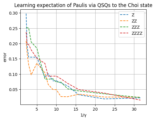
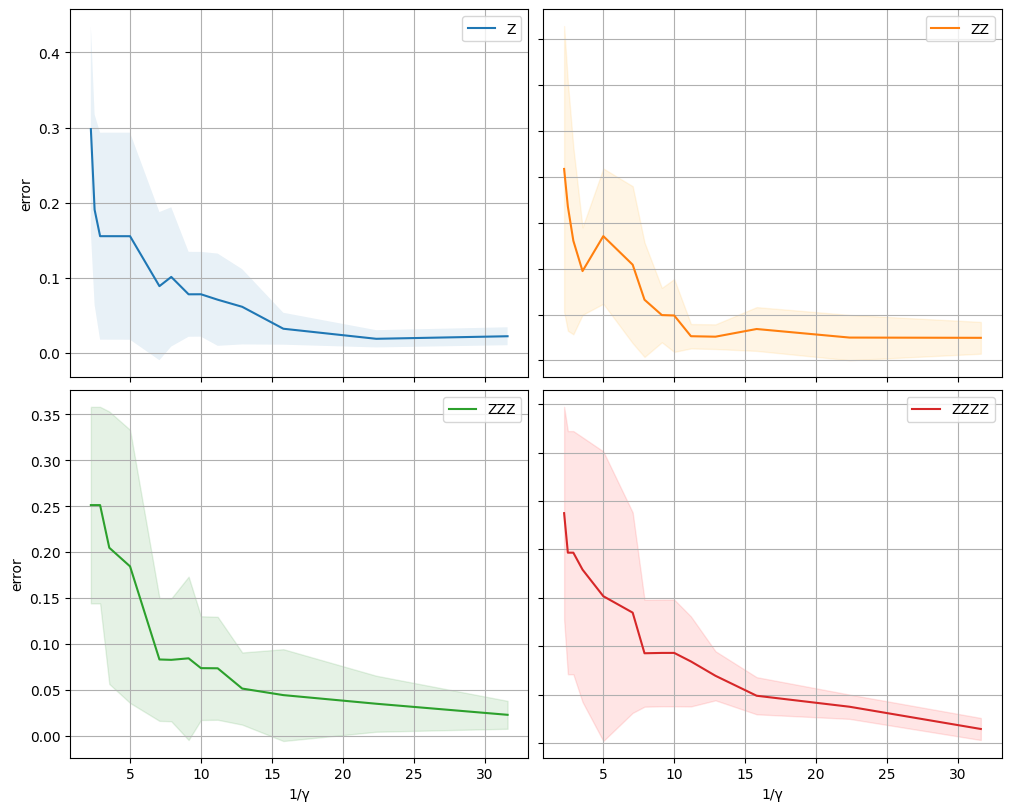
Figure 1: Average performance of the Goldreich-Levin algorithm implemented with quantum statistical queries to the Choi-Jamiolkowski state. We tested the algorithm on 10 random 4-qubit random unitaries, in predicting the absolute value of the outcome of $Z$ observables on the unitary evolution of computational basis states. Each random unitary consists in 2 layers of Haar-random gates. We plotted the average error as a function of $1/\gamma$, i.e. the inverse of the threshold of Algorithm 2. We set the tolerance of the quantum statistical queries as $\gamma^{2}/4$.

4 Exponential separations between QSQs and Choi state access

We will now prove a lower bound for learning Choi states with QSQs, and derive from it an exponential separation between learning unitaries from QSQs and learning unitaries with Choi state access. To this end, we combine Lemma 2.1 with an argument given in [11] and based on the following concept class (of classical functions):

$$\mathcal{C}=\left\{f_{A}:\{0,1\}^{n}\rightarrow\{0,1\},f_{A}(x)=x^{\top}Ax\mod 2\;\;|\;\;A\in\mathbb{F}_{2}^{n\times n}\right\}$$ (68)

Theorem 4.1 (Hardness of learning phase oracles).

The concept class of phase oracle unitaries $V_{f_{A}}$, i.e.

$$\{V_{f_{A}}\;\;|\;\;A\in\mathbb{F}_{2}^{n\times n}\}$$ (69)

requires $2^{\Omega(n)}$ many quantum statistical queries to $\mathsf{QStat}_{V_{f_{A}}}$ of tolerance $1/\mathrm{poly}(n)$ to be learnt below distance $D<0.05$ with high probability.

Proof.

Our proof is based on the one of ([11], Theorem 17). Their statement is analogous, with the class of quantum examples $\ket{\psi_{f_{A}}}$ replacing that of unitaries $V_{f_{A}}$. The only things we need to prove are the following

$$\||{v(V_{f_{A}})}\rangle\langle{v(V_{f_{A}})}|-\mathbb{E}_{B}|{v(V_{f_{B}})}\rangle\langle{v(V_{f_{B}})}|\|_{\mathrm{tr}}\geq 1-\sqrt{17/32},$$ (70)

$$\max_{M:\|M\|=1}\mathbb{V}_{A}\mathrm{Tr}\left[M|{v(V_{f_{A}})}\rangle\langle{v(V_{f_{A}})}|\right]=2^{-\Omega(n)}$$ (71)

and then the result follows from ([11], Theorem 16). The first line follows by checking that

$$\||{v(V_{f_{A}})}\rangle\langle{v(V_{f_{A}})}|-\mathbb{E}_{B}|{v(V_{f_{B}})}\rangle\langle{v(V_{f_{B}})}|\|_{\mathrm{tr}}=\||{\psi_{f_{A}}}\rangle\langle{\psi_{f_{A}}}|-\mathbb{E}_{B}|{\psi_{f_{B}}}\rangle\langle{\psi_{f_{B}}}|\|_{\mathrm{tr}}\geq 1-\sqrt{17/32},$$ (72)

Where the lower bound is proven in [11]. As for the variance, we notice the following

$$\mathbb{V}_{A}\mathrm{Tr}\left[M|{v(V_{f_{A}})}\rangle\langle{v(V_{f_{A}})}|\right]= \mathbb{E}_{A}\mathrm{Tr}\left[M|{v(V_{f_{A}})}\rangle\langle{v(V_{f_{A}})}|^{2}\right]-\mathbb{E}_{A}\mathrm{Tr}\left[M|{v(V_{f_{A}})}\rangle\langle{v(V_{f_{A}})}|\right]^{2}$$ (73)

$$= \mathbb{E}_{A}\mathrm{Tr}\left[M^{\prime}|{\psi_{f_{A}}}\rangle\langle{\psi_{f_{A}}}|^{2}\right]-\mathbb{E}_{A}\mathrm{Tr}\left[M^{\prime}|{\psi_{f_{A}}}\rangle\langle{\psi_{f_{A}}}|\right]^{2}=2^{-\Omega(n)},$$ (74)

where the observable $M^{\prime}$ is the one obtained following the procedure of Lemma 2.1 and the upper bound follows again from [11]. ∎

We also provide a double exponential lower bound for testing properties of channels, which also comes as a direct consequence of a lower bound for testing purity of states given in [11]. First, recall that the unitarity [38, 39] of a quantum channel is defined as

$$u(\mathcal{N}):=\frac{2^{n}}{2^{n}-1}\mathbb{E}_{\ket{\psi}\sim\mu_{n}}\mathrm{Tr}\left[\mathcal{N}(|{\psi}\rangle\langle{\psi}|)^{2}\right]-\frac{2^{n}}{2^{n}-1}\mathrm{Tr}\left[\mathcal{N}\left(\frac{I}{2^{n}}\right)^{2}\right]$$ (75)

Theorem 4.2 (Hardness of testing unitarity).

Let $\mathcal{A}$ be an algorithm that estimates with high probability the unitarity of a quantum channel $\mathcal{N}$ with error smaller than $0.24$ using $\mathsf{Qstat}_{\mathcal{N}}$ queries with tolerance at least $\tau$. Then $\mathcal{A}$ must make at least $2^{\Omega(\tau^{2}2^{n})}$ such queries.

Proof.

Assume the existence of an algorithm $\mathcal{A}$ contradicting the statement of the theorem. We will prove the theorem by contradiction, by first showing that the unitarity is closely related to the purity of the Choi state $\mathcal{J}(\mathcal{N})$, and then applying the lower bound for testing purity given in ([11], Theorem 25).

$$\mathbb{E}_{\ket{\psi}\sim\mu_{n}}\mathrm{Tr}\left[\mathcal{N}(|{\psi}\rangle\langle{\psi}|)^{2}\right]=\mathbb{E}_{\ket{\psi}\sim\mu_{n}}\mathrm{Tr}\left[\mathbb{F}\mathcal{N}^{\otimes 2}(|{\psi}\rangle\langle{\psi}|^{\otimes 2})\right]$$ (76)

$$=\mathrm{Tr}\left[\mathbb{F}\mathcal{N}^{\otimes 2}(\mathbb{E}_{\ket{\psi}\sim\mu_{n}}|{\psi}\rangle\langle{\psi}|^{\otimes 2})\right]=\mathrm{Tr}\left[\mathbb{F}\mathcal{N}^{\otimes 2}\left(\frac{\mathbb{I}+\mathbb{F}}{2^{n}(2^{n}+1)}\right)\right]$$ (77)

$$=\mathrm{Tr}\left[\mathbb{F}\mathcal{N}^{\otimes 2}\left(\frac{\mathbb{F}}{2^{n}(2^{n}+1)}\right)\right]+\mathrm{Tr}\left[\mathbb{F}\mathcal{N}^{\otimes 2}\left(\frac{\mathbb{I}}{2^{n}(2^{n}+1)}\right)\right]$$ (78)

$$=\mathrm{Tr}\left[\mathbb{F}\mathcal{N}^{\otimes 2}\left(\frac{\mathbb{F}}{2^{n}(2^{n}+1)}\right)\right]+\mathrm{Tr}\left[\mathcal{N}\left(\frac{I}{2^{n}}\right)^{2}\right]\frac{2^{n}}{(2^{n}+1)}$$ (79)

Then we can rearrange the unitarity as follows

$$u(\mathcal{N})=\frac{1}{4^{n}-1}\mathrm{Tr}\left[\mathbb{F}\mathcal{N}^{\otimes 2}\left({\mathbb{F}}\right)\right]-\frac{1}{4^{n}-1}\mathrm{Tr}\left[\mathcal{N}\left(\frac{I}{2^{n}}\right)^{2}\right]$$ (80)

We can also use the Kraus representation $\mathcal{N}(\cdot)=\sum_{\ell}K_{\ell}(\cdot)K_{\ell}^{\dagger}$ and write

$$\mathrm{Tr}\left[\mathbb{F}\mathcal{N}^{\otimes 2}\left({\mathbb{F}}\right)\right]=\sum_{\ell,\ell^{\prime}}\mathrm{Tr}\left[\mathbb{F}(K_{\ell}\otimes K_{\ell^{\prime}}){\mathbb{F}}(K_{\ell}^{\dagger}\otimes K_{\ell^{\prime}}^{\dagger})\right]$$ (81)

$$=\sum_{\ell,\ell^{\prime}}|\mathrm{Tr}[K_{\ell}K_{\ell^{\prime}}^{\dagger}]|^{2}=4^{n}\mathrm{Tr}[J(\mathcal{N})^{2}],$$ (82)

where the last two identities are proven in ([14], Eqs. 160-164). Putting all together, we obtain:

$$\frac{4^{n}}{4^{n}-1}\mathrm{Tr}[J(\mathcal{N})^{2}]-\frac{1}{4^{n}-1}\leq u(\mathcal{N})\leq\frac{4^{n}}{4^{n}-1}\mathrm{Tr}[J(\mathcal{N})^{2}]$$ (83)

Thus the unitarity of $\mathcal{N}$ and the purity of $\mathcal{J}(\mathcal{N})$ are within an exponentially small additive terms. Then the algorithm $\mathcal{A}$ would estimate the purity of $\mathcal{J}(\mathcal{N})$ with error smaller than $0.24+1/(4^{n}-1)$ with less than $2^{\Omega(\tau^{2}2^{n})}$ queries, contradicting ([11], Theorem 25). ∎

5 Application: Classical Surrogates

In this section we discuss a potential application of our results to quantum machine learning. We will consider particularly variational quantum algorithms for approximating a classical function $f:\mathcal{X}\rightarrow\mathbb{R}$. For a broad class of such algorithms [40, 41], the prediction phase can be cast as follows: the input $\boldsymbol{x}\in\mathcal{X}$ is encoded into a quantum state with a suitable feature map $\boldsymbol{x}\mapsto\rho(\boldsymbol{x})$, which evolves according to a parametric channel $\mathcal{U}_{\boldsymbol{\theta}}$ and subsequently is measured with a local observable $O$. Hence, the parametric circuit induces a hypothesis function $h(\cdot)$, which associates $\boldsymbol{x}$ to the following label

$$h(\boldsymbol{x})=\mathrm{Tr}[O\mathcal{U}_{\boldsymbol{\theta}}(\rho(\boldsymbol{x}))].$$ (84)

Thus, given a distribution $\mathcal{D}$ over $\mathcal{X}$, the goal is to find a parameter $\boldsymbol{\theta}^{*}$ satisfying the following:

$$\mathbb{E}_{\boldsymbol{x}\sim\mathcal{D}}|h(\boldsymbol{x})-f(\boldsymbol{x})|=\mathbb{E}_{\boldsymbol{x}\sim\mathcal{D}}|\mathrm{Tr}[O\mathcal{U}_{\boldsymbol{\theta}^{*}}(\rho(\boldsymbol{x}))]-f(\boldsymbol{x})|\leq\varepsilon,$$ (85)

where $\varepsilon$ is a small positive constant. Given a set of examples $(\boldsymbol{x}_{1},f(\boldsymbol{x}_{1})),(\boldsymbol{x}_{2},f(\boldsymbol{x}_{2})),\dots,(\boldsymbol{x}_{m},f(\boldsymbol{x}_{m}))$ one can then train this model in a hybrid fashion and select a parameter $\boldsymbol{\theta}$. Then the label of an unseen instance $\boldsymbol{x}_{m+1}$ can be predicted with accuracy $\varepsilon$ preparing $O(\varepsilon^{-2})$ copies of the state $\mathcal{U}_{\boldsymbol{\theta}}(\rho(\boldsymbol{x}))$ and measuring the observable $O$.

A recent line of research showed that, in some cases, one can fruitfully perform the prediction phase with a purely classical algorithm, that goes under the name of classical surrogate [21]. So far, the proposed approaches rely on the classical shadow tomography [22] and the Fourier analysis of real functions [42, 21], which can be applied to the general expression of quantum models as trigonometric polynomials. Here we argue that the QSQ learning framework can find application in the quest for surrogate models, introducing more flexibility in the surrogation process. Particularly, [22] resorts to a flipped model of quantum circuit where the parameter $\boldsymbol{\theta}$ is encoded in a quantum state, subsequently measured by a variational measurements depending on the $\boldsymbol{x}$. While this model can provide quantum advantage for specific tasks, it would be interesting to obtain similar results beyond the flipped circuit model, and specifically for the setting where the instance $\boldsymbol{x}$ is encoded before the parameter $\boldsymbol{\theta}$. This goal can be achieved through the algorithms discussed in the present paper, since they do not require the unitary to be a flipped a circuit. However, the distance over unitaries we adopted brings accuracy guarantees for the prediction only when the input state is sampled from a locally scrambled ensemble. Thus, we need to extend the definition given in [21] to incorporate the input distribution $\mathcal{D}$.

Definition 5.1 (Worst-case and average-case surrogate models).

Let $\varepsilon\geq 0$ and $0\leq\delta\leq 1$. A hypothesis class of quantum learning models $\mathcal{F}$ has a worst-case $(\varepsilon,\delta)$-classical surrogate if there exists a process $\mathcal{S}$ that upon input of a learning model $f\in\mathcal{F}$ produces a classical model $g\in\mathcal{G}$ such that

$$\Pr\left[\sup_{\boldsymbol{x}\in\mathcal{X}}\|f(\boldsymbol{x})-g(\boldsymbol{x})\|\leq\varepsilon\right]\geq 1-\delta,$$ (86)

for a suitable norm on the output space $\mathcal{Y}$. Similarly, we say that $\mathcal{F}$ has an average-case $(\varepsilon,\delta)$-classical surrogate if there exists a process $\mathcal{S}$ that upon input of a learning model $f\in\mathcal{F}$ produces a classical model $g\in\mathcal{G}$ such that

$$\Pr[\mathbb{E}_{\boldsymbol{x}\sim\mathcal{D}}\|f(\boldsymbol{x})-g(\boldsymbol{x})\|\leq\varepsilon]\geq 1-\delta.$$ (87)

The process $\mathcal{S}$ must be efficient in the size of the quantum learning model, the error bound $\varepsilon$ and the failure probability $\delta$.

In particular, it is easy to see that if the conditional distribution of the states $\rho(\boldsymbol{x})$ is locally scrambled, then we can produce an average-case classical surrogate of $f(\boldsymbol{x})=\mathrm{Tr}[O\mathcal{U}_{\boldsymbol{\theta}}\rho(\boldsymbol{x})]$ via QSQs by means of Theorems 3.2,3.3,3.5 . For instance, if $\mathcal{D}$ is the uniform distribution over $[6]^{n}$, the ensemble $\{\ket{\phi(\boldsymbol{x})}\}_{\boldsymbol{x}}$ defined as follows is locally scrambled. We have:

$$\ket{\phi(\boldsymbol{x})}=\bigotimes_{i=1}^{n}\ket{\phi({x}_{i})}\;\;\;\text{where}\;\;\;\ket{\phi({x}_{i})}=\begin{cases}\ket{0}&\text{ if ${x}_{i}=1$}\\ \ket{1}&\text{ if ${x}_{i}=2$}\\ \ket{+}&\text{ if ${x}_{i}=3$}\\ \ket{-}&\text{ if ${x}_{i}=4$}\\ \ket{y_{+}}&\text{ if ${x}_{i}=5$}\\ \ket{y_{-}}&\text{ if ${x}_{i}=6$}.\end{cases}$$ (88)

While this example is just meant to motivate our definition of average-case surrogate models, the quest for quantum encodings mapping a target distribution over $\mathcal{X}$ to a locally scrambled distribution would be of primary importance for the design of surrogation processes. We also remark that worst-case surrogate models could be found by means of the quantum Goldreich-Levin algorithm, and in particular by exploiting the fact the unitary evolution in the Heisenberg picture of a Pauli string $P\in\mathcal{P}_{n}$, i.e. $\mathcal{U}^{\dagger}_{\boldsymbol{\theta}}(P)={U}^{\dagger}_{\boldsymbol{\theta}}P{U}_{\boldsymbol{\theta}}$, is a quantum Boolean function. This follows from the fact that the accuracy guarantees of Theorem 3.5 expressed in Hilbert-Schimdt distance can be transferred to an arbitrary state, as noted in Remark 3.2. This will allow learning $\mathcal{U}^{\dagger}_{\boldsymbol{\theta}}(P)$, up to a multiplicative sign, and hence to predict functions of the form

$$h(\boldsymbol{x})=\left|\mathrm{Tr}[P\mathcal{U}_{\boldsymbol{\theta}}(\rho(\boldsymbol{x}))]\right|.$$ (89)

References

• Chuang and Nielsen [1997] Isaac L Chuang and Michael A Nielsen. Prescription for experimental determination of the dynamics of a quantum black box. Journal of Modern Optics, 44(11-12):2455–2467, 1997.
• Gutoski and Johnston [2014] Gus Gutoski and Nathaniel Johnston. Process tomography for unitary quantum channels. Journal of Mathematical Physics, 55(3), 2014.
• Montanaro and Osborne [2010] Ashley Montanaro and Tobias J Osborne. Quantum boolean functions. Chicago Journal OF Theoretical Computer Science, 1:1–45, 2010.
• Chen et al. [2023] Thomas Chen, Shivam Nadimpalli, and Henry Yuen. Testing and learning quantum juntas nearly optimally. In Proceedings of the 2023 Annual ACM-SIAM Symposium on Discrete Algorithms (SODA), pages 1163–1185. SIAM, 2023.
• Bao and Yao [2023] Zongbo Bao and Penghui Yao. Nearly optimal algorithms for testing and learning quantum junta channels. arXiv preprint arXiv:2305.12097, 2023.
• Fanizza et al. [2022] Marco Fanizza, Yihui Quek, and Matteo Rosati. Learning quantum processes without input control. arXiv preprint arXiv:2211.05005, 2022.
• Huang et al. [2022] Hsin-Yuan Huang, Sitan Chen, and John Preskill. Learning to predict arbitrary quantum processes. arXiv preprint arXiv:2210.14894, 2022.
• Montanaro and de Wolf [2013] Ashley Montanaro and Ronald de Wolf. A survey of quantum property testing. arXiv preprint arXiv:1310.2035, 2013.
• Preskill [2018] John Preskill. Quantum computing in the nisq era and beyond. Quantum, 2:79, 2018.
• Arunachalam et al. [2020] Srinivasan Arunachalam, Alex B Grilo, and Henry Yuen. Quantum statistical query learning. arXiv preprint arXiv:2002.08240, 2020.
• Arunachalam et al. [2023] Srinivasan Arunachalam, Vojtech Havlicek, and Louis Schatzki. On the role of entanglement and statistics in learning. arXiv preprint arXiv:2306.03161, 2023.
• Kearns [1998] Michael Kearns. Efficient noise-tolerant learning from statistical queries. Journal of the ACM (JACM), 45(6):983–1006, 1998.
• Caro et al. [2023a] Matthias C Caro, Marcel Hinsche, Marios Ioannou, Alexander Nietner, and Ryan Sweke. Classical verification of quantum learning. arXiv preprint arXiv:2306.04843, 2023a.
• Quek et al. [2022] Yihui Quek, Daniel Stilck França, Sumeet Khatri, Johannes Jakob Meyer, and Jens Eisert. Exponentially tighter bounds on limitations of quantum error mitigation, 2022. URL https://arxiv.org/abs/2210.11505.
• Du et al. [2021] Yuxuan Du, Min-Hsiu Hsieh, Tongliang Liu, Dacheng Tao, and Nana Liu. Quantum noise protects quantum classifiers against adversaries. Physical Review Research, 3(2), may 2021. doi: 10.1103/physrevresearch.3.023153. URL https://doi.org/10.1103%2Fphysrevresearch.3.023153.
• Hinsche et al. [2023] M Hinsche, M Ioannou, A Nietner, J Haferkamp, Y Quek, D Hangleiter, J-P Seifert, J Eisert, and R Sweke. One t gate makes distribution learning hard. Physical Review Letters, 130(24):240602, 2023.
• Gollakota and Liang [2022] Aravind Gollakota and Daniel Liang. On the hardness of pac-learning stabilizer states with noise. Quantum, 6:640, 2022.
• Nietner et al. [2023] Alexander Nietner, Marios Ioannou, Ryan Sweke, Richard Kueng, Jens Eisert, Marcel Hinsche, and Jonas Haferkamp. On the average-case complexity of learning output distributions of quantum circuits. arXiv preprint arXiv:2305.05765, 2023.
• Angrisani and Kashefi [2022] Armando Angrisani and Elham Kashefi. Quantum local differential privacy and quantum statistical query model. arXiv preprint arXiv:2203.03591, 2022.
• Caro et al. [2023b] Matthias C Caro, Hsin-Yuan Huang, Nicholas Ezzell, Joe Gibbs, Andrew T Sornborger, Lukasz Cincio, Patrick J Coles, and Zoë Holmes. Out-of-distribution generalization for learning quantum dynamics. Nature Communications, 14(1):3751, 2023b.
• Schreiber et al. [2023] Franz J Schreiber, Jens Eisert, and Johannes Jakob Meyer. Classical surrogates for quantum learning models. Physical Review Letters, 131(10):100803, 2023.
• Jerbi et al. [2023] Sofiene Jerbi, Casper Gyurik, Simon C Marshall, Riccardo Molteni, and Vedran Dunjko. Shadows of quantum machine learning. arXiv preprint arXiv:2306.00061, 2023.
• Atıcı and Servedio [2007] Alp Atıcı and Rocco A Servedio. Quantum algorithms for learning and testing juntas. Quantum Information Processing, 6(5):323–348, 2007.
• Caro [2020] Matthias C Caro. Quantum learning boolean linear functions wrt product distributions. Quantum Information Processing, 19(6):172, 2020.
• Kanade et al. [2019] V Kanade, A Rocchetto, and S Severini. Learning dnfs under product distributions via $\mu$-biased quantum fourier sampling. Quantum Information and Computation, 19(15&16), 2019.
• Mele [2023] Antonio Anna Mele. Introduction to haar measure tools in quantum information: A beginner’s tutorial. arXiv preprint arXiv:2307.08956, 2023.
• Choi [1975] Man-Duen Choi. Completely positive linear maps on complex matrices. Linear Algebra and its Applications, 10(3):285–290, 1975. ISSN 0024-3795. doi: https://doi.org/10.1016/0024-3795(75)90075-0. URL https://www.sciencedirect.com/science/article/pii/0024379575900750.
• Jamiołkowski [1972] A. Jamiołkowski. Linear transformations which preserve trace and positive semidefiniteness of operators. Reports on Mathematical Physics, 3(4):275–278, 1972. ISSN 0034-4877. doi: https://doi.org/10.1016/0034-4877(72)90011-0. URL https://www.sciencedirect.com/science/article/pii/0034487772900110.
• Low [2009] Richard A Low. Learning and testing algorithms for the clifford group. Physical Review A, 80(5):052314, 2009.
• Wang [2011] Guoming Wang. Property testing of unitary operators. Physical Review A, 84(5):052328, 2011.
• Rouzé et al. [2022] Cambyse Rouzé, Melchior Wirth, and Haonan Zhang. Quantum talagrand, kkl and friedgut’s theorems and the learnability of quantum boolean functions, 2022.
• O’Donnell [2021] Ryan O’Donnell. Analysis of boolean functions. arXiv preprint arXiv:2105.10386, 2021.
• Bshouty and Jackson [1995] Nader H Bshouty and Jeffrey C Jackson. Learning dnf over the uniform distribution using a quantum example oracle. In Proceedings of the eighth annual conference on Computational learning theory, pages 118–127, 1995.
• Caro [2022] Matthias C Caro. Learning quantum processes and hamiltonians via the pauli transfer matrix. arXiv preprint arXiv:2212.04471, 2022.
• Coles et al. [2019] Patrick J Coles, M Cerezo, and Lukasz Cincio. Strong bound between trace distance and hilbert-schmidt distance for low-rank states. Physical Review A, 100(2):022103, 2019.
• Melkani et al. [2020] Abhijeet Melkani, Clemens Gneiting, and Franco Nori. Eigenstate extraction with neural-network tomography. Phys. Rev. A, 102:022412, Aug 2020. doi: 10.1103/PhysRevA.102.022412. URL https://link.aps.org/doi/10.1103/PhysRevA.102.022412.
• Yu and Wei [2023] Nengkun Yu and Tzu-Chieh Wei. Learning marginals suffices! arXiv preprint arXiv:2303.08938, 2023.
• Wallman et al. [2015] Joel Wallman, Chris Granade, Robin Harper, and Steven T Flammia. Estimating the coherence of noise. New Journal of Physics, 17(11):113020, 2015.
• Carignan-Dugas et al. [2019] Arnaud Carignan-Dugas, Joel J Wallman, and Joseph Emerson. Bounding the average gate fidelity of composite channels using the unitarity. New Journal of Physics, 21(5):053016, 2019.
• Schuld and Killoran [2019] Maria Schuld and Nathan Killoran. Quantum machine learning in feature hilbert spaces. Physical review letters, 122(4):040504, 2019.
• Schuld [2021] Maria Schuld. Supervised quantum machine learning models are kernel methods. arXiv preprint arXiv:2101.11020, 2021.
• Landman et al. [2022] Jonas Landman, Slimane Thabet, Constantin Dalyac, Hela Mhiri, and Elham Kashefi. Classically approximating variational quantum machine learning with random fourier features. In The Eleventh International Conference on Learning Representations, 2022.