Variational Coherent Quantum Annealing

Abstract

We present a hybrid classical-quantum computing paradigm where the quantum part strictly runs within the coherence time of a quantum annealer, a method we call variational coherent quantum annealing (VCQA). It involves optimizing the schedule functions governing the quantum dynamics by employing a piecewise family of tailored functions. We also introduce auxiliary Hamiltonians that vanish at the beginning and end of the evolution to increase the energy gap during the process, subsequently reducing the algorithm times. We develop numerical tests using $z$-local terms as the auxiliary Hamiltonian while considering linear, cyclic, and star connectivity. Moreover, we test our algorithm for a non-stoquastic Hamiltonian such as a Heisenberg chain, showing the potential of the VCQA proposal in different scenarios. In this manner, we achieve a substantial reduction in the ground-state error with just six variational parameters and a duration within the device coherence times. Therefore, the proposed VCQA paradigm offers exciting prospects for current quantum annealers.

I Introduction

Adiabatic quantum computing (AQC) and its realization as quantum annealers (QAs) have been active research areas in recent years, offering potential solutions to a wide range of quadratic unconstrained binary optimization (QUBO) problems [1, 2, 3, 4, 5, 6, 7, 8, 9, 10, 11]. While AQC is a universal computation paradigm equivalent to gate-based quantum computing [12], the experimental implementation of universal AQC remains a significant challenge. This is primarily due to the complex analog evolution process it involves, which currently limits the range of solvable problems to a very specific set. In this context, QUBO problems, which have been implemented in superconducting circuits [13, 14] and nuclear magnetic resonance-based systems [15, 16], provide one feasible avenue for the implementation of AQC. In this line, theoretical proposals are also exploring this paradigm in other platforms, such as neutral atoms [17, 18].

Quantum annealers, such as those developed by D-Wave [19], are specifically designed to solve spin-glass Hamiltonians. While these quantum annealers can only manage a limited subset of algorithms, their ability to handle any problem formulated in QUBO form is noteworthy. This is significant because any classical problem can be approximated using a QUBO formulation, suggesting that current quantum annealers pave the way for quantum optimization of multivariable functions. The procedure involves encoding classical problems into an optimization function, approximating it with polynomial terms, and expressing variables in binary form. Each classical binary variable is then mapped to a quantum spin operator. High-order polynomial terms can be managed using only linear and quadratic terms by introducing additional auxiliary qubits [20, 21]. This allows a classical optimization problem to be written in its QUBO form, which is equivalent to a spin-glass Hamiltonian [22, 23, 24].

The versatility of the QUBO formulation has enabled the application of QAs in various domains, including quantum finance, quantum chemistry, and machine learning [25, 26, 27, 28, 29, 30, 31, 32, 33]. However, the quantum nature of these devices has raised questions about their advantage over classical computation methods [34, 35]. Critics often point to the time evolution inherent in adiabatic processes, which usually exceeds the coherence time of the physical devices. To address this, protocols related to quantum control have been proposed, focusing primarily on optimizing the schedule function that interpolates between the initial and final Hamiltonians during the adiabatic evolution [36, 37, 38, 39, 40, 41, 42, 43, 44]. While these efforts have reduced the total time required for the adiabatic algorithm, implementing them on current devices remains challenging, and in some cases, the evolution time still exceeds the coherence time of current devices. Thus, there is a need for an experimental method to parametrize a wide range of schedule functions for optimizing the accuracy of current quantum annealers.

In this work, we introduce a variational coherent quantum annealing (VCQA) algorithm that enhances the common annealing protocol by incorporating a third auxiliary Hamiltonian. The VCQA protocol is composed of three elements; the initial Hamiltonian, the final Hamiltonian, and the auxiliary Hamiltonian. Each of these elements has its own independent schedule function with initial and final conditions. We parametrize each schedule function using a piece-wise cubic interpolator, as previously proposed in ref. [44]. The role of the auxiliary Hamiltonian is to enlarge the time-dependent energy spectrum which improves the accuracy of the VCQA algorithm. We have designed the VCQA protocol to be compatible with existing quantum annealers. It utilizes only the available interactions, specifically employing $z$-local terms as auxiliary Hamiltonians and operates within a time frame that is less than the coherence time of the device. We have numerically tested our proposal using various QUBO Hamiltonians of up to 10 sites, as well as a non-stoquastic example of a Heisenberg chain, even if the last cannot be addressed with the current QAs, it is interesting to show the potencial of VCQA protocol. With just two variational parameters per schedule function (a total of six parameters), we demonstrate a significant reduction in error compared to traditional ramp schedule functions.

II Variational Coherent Quantum Annealing algorithm

We consider a general adiabatic evolution described by the time-dependent Hamiltonian,

$$H(t)=F_{1}(t/T)H_{i}+F_{2}(t/T)H_{f}+F_{3}(t/T)H_{aux},$$ (1)

with $F_{1}(0)=F_{2}(1)=1$, and $F_{1}(1)=F_{2}(0)=F_{3}(0)=F_{3}(1)=0$. $H_{i}$ is the initial Hamiltonian whose ground state is easy to prepare. In general, for quantum annealers, $H_{i}$ takes the form

$$H_{i}=\epsilon\sum_{j=1}^{N}\sigma^{x}_{j},$$ (2)

whose ground state is $\bigotimes_{j=1}^{N}|-\rangle_{j}$, where $(|0\rangle_{j}-|1\rangle_{j})/\sqrt{2}$. $H_{f}$ is the final Hamiltonian whose ground state codifies the solution of an optimization problem. In general, for quantum annealers $H_{f}$ corresponds to a spin-glass Hamiltonian given by

$$H_{f}=\sum_{j=1}^{N}\omega_{j}\sigma^{z}_{j}+\sum_{j,k;j>k}g_{j,k}\sigma^{z}_{j}\sigma^{z}_{k}.$$ (3)

As previously stated, the ground state of a spin-glass Hamiltonian can encode the solution to any QUBO problem. Finally, $H_{aux}$ is an auxiliary Hamiltonian that serves a crucial role in our VCQA protocol by altering the energy landscape during the evolution process to optimize performance. The specific form of $H_{aux}$ will be discussed in a later section.

To optimize the functions $F_{1}$, $F_{2}$, and $F_{3}$, we use a parametrization approach based on cubic piece-wise interpolation through mobile points, which serve as variational parameters. As indicated in Eq. (1), we need to parametrize three functions. If we use $n_{j}$ parameters for the function $F_{j}$, then our cost function will depend on $\sum_{j=1}^{3}n_{j}$ parameters.

II.1 Parametrization of the schedule function

We use a piece-wise interpolator to parametrize the schedule functions, with the set of points defined by our parameter space. To ensure the schedule function is experimentally feasible, we impose two conditions: continuity in the function and its first derivative (smoothness). These conditions guarantee that the resulting function will not exhibit abrupt changes, makig it more reasonable for implementation.

Additionally, we ensure that the schedule function does not exceed a maximum value or fall below a minimum one. These boundary values are determined by the experimental capabilities of the physical devices that would be used to generate our schedule functions. To meet this requirement, we enforce a monotonic condition between adjacent points on the piece-wise interpolator. This implies that any boundary in the schedule function can be addressed by bounding the points (parameters) during the interpolation process.

A method that satisfies these three conditions is the piece-wise cubic Hermite interpolator, as demonstrated in ref. [45]. The method is outlined as follows; consider a set of $N_{j}$ parameters, denoted as ${\vec{p}_{j}=(p_{j,1},p_{j,2},...,p_{j,N_{j}})}$. These parameters define the $N_{j}+2$ points $\mathcal{P}=\{(0,p_{j,0}),(\Delta_{j},p_{j,1}),(2\Delta_{j},p_{j,1}),...,(1,p_{j,f})\}$, where $\Delta_{j}=1/(N_{j}+1)$. The values $p_{j,0}$ and $p_{j,f}$ are determined by the boundary conditions over the schedule function $F_{j}$. For simplicity, we have chosen equally-spaced points. Using the set of point $\mathcal{P}$, we define the schedule function $F_{j}$ as follows

$$F_{j}(x)= h_{j,k,0}(x)p_{j,k}+h_{j,k,1}(x)p_{j,k+1}$$ (4)

$$+h_{j,k,2}(x)\Delta_{j}m_{j,k}+h_{j,k,3}(x)\Delta_{j}m_{j,k+1},\,$$

with $k\Delta_{j}\leq x\leq(k+1)\Delta_{j}$. The functions $h_{j,k,\ell}$ are given by

$$h_{j,k,0} = \left[1+2\left(\frac{x-k\Delta_{j}}{\Delta_{j}}\right)\right]\left[1-\left(\frac{x-k\Delta_{j}}{\Delta_{j}}\right)\right]^{2},$$

$$h_{j,k,1} = \left(\frac{x-k\Delta_{j}}{\Delta_{j}}\right)^{2}\left[3-2\left(\frac{x-k\Delta_{j}}{\Delta_{j}}\right)\right],$$

$$h_{j,k,2} = \left(\frac{x-k\Delta_{j}}{\Delta_{j}}\right)\left[1-\left(\frac{x-k\Delta_{j}}{\Delta_{j}}\right)\right]^{2},$$

$$h_{j,k,3} = \left(\frac{x-k\Delta_{j}}{\Delta_{j}}\right)^{2}\left[1-\left(\frac{x-k\Delta_{j}}{\Delta_{j}}\right)\right],$$ (5)

and the slopes $m_{k}$ at $x=k\Delta_{j}$ and $m_{k+1}$ at $x=(k+1)\Delta_{j}$ are selected according to

$$m_{j,k}=\frac{2(p_{j,k+1}-p_{j,k})(p_{j,k+2}-p_{j,k+1})}{\Delta_{j}(p_{j,k+2}-p_{j,k})}$$ (6)

if and only if $(p_{j,k+1}-p_{j,k})(p_{j,k+2}-p_{j,k+1})>0$, otherwise $m_{j,k}=0$. Also, as previously stated, we have $p_{min}<F_{j}(x)<p_{max}$, where $p_{min}(p_{max})$ is the minimum (maximum) between the all the points $p_{j,k}$, and is related to the range of values that the experimental device can generate.

II.2 Auxiliary Hamiltonian

Our algorithm hinges on the utilization of an auxiliary Hamiltonian. This additional term serves to alter the energy spectrum of the Hamiltonian during its evolution. Given our objective to propose a protocol that is feasible for experimentation, we restrict our consideration to local terms only. Since in the spin glass Hamiltonian each spin has a distinct frequency, denoted as $\omega_{j}$, for the auxiliary Hamiltonian we will consider local terms of the form

$$H_{aux}=\sum_{j}\omega_{j}\sigma_{j}^{\alpha},$$ (7)

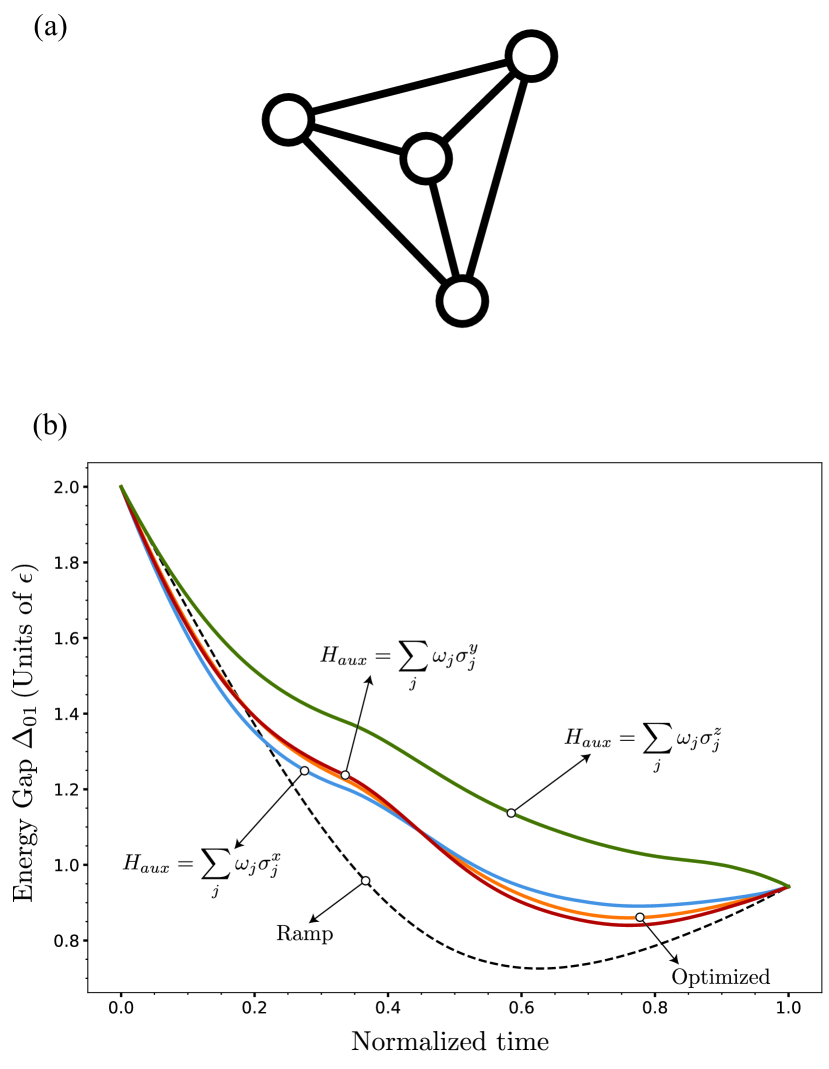
Figure 1: (a) Depiction of a fully connected graph comprising four sites, utilized to evaluate the impact of the auxiliary Hamiltonian. (b) Energy Gap $\Delta_{01}$ as a function of normalized time, for different auxiliary Hamiltonians.

where $\alpha=\{x,y,z\}$. To analyze the impact of this auxiliary Hamiltonian on the energy gap, we examine a fully connected configuration comprising four sites, depicted in Figure 1 (a). This configuration serves as a test for each auxiliary Hamiltonian. We focus on the Hamiltonian outlined in Eq. (3), where $\omega_{j}$ and $g_{j,k}$ are randomly selected within the range $[0,1]$.

In Fig. 1 (b), we plot the average energy gap, $\Delta_{01}$, between the ground and first excited state for various strategies across 100 different random instances. First, we consider the standard ramp schedule function, defined by $F_{1}=1-t/T$, $F_{2}=t/T$, and $F_{3}=0$ (dashed line). Second, we perform the optimization of the schedule functions without an auxiliary Hamiltonian (orange line), where we have used two parameters per schedule function, amounting to four parameters in total. Finally, we consider the optimization of schedule functions including auxiliary Hamiltonians of local operators in the $x$-axis (blue line), $y$-axis (red line) and $z$-axis (green line). In these last three strategies, we need to consider the optimization over six parameters since we incorporated an extra schedule function to drive the auxiliary Hamiltonian.

We can observe that the ramp strategy typically displays a minimum gap at approximately 0.6 in normalized time, a characteristic that other strategies attempt to avoid. Optimized schedule functions for local interactions along the $x$ and $y$ axes, as well as schedules devoid of an auxiliary Hamiltonian, exhibit a region where the gap is lower than that of the ramp case, located at the beginning of the evolution. This is because of the limited number of parameters involved in the optimization process.

Interestingly, the $z$-local auxiliary Hamiltonian consistently outperforms other strategies in terms of enlarging the energy gap, and it is the sole strategy that exhibits a monotonic behavior of the gap during the evolution. This suggests that when considering only local terms for the auxiliary Hamiltonian, the $z$-local auxiliary Hamiltonian is the most effective strategy.

In the case of the $z$-local strategy, the frequency of each qubit in the auxiliary Hamiltonian matches the local term of the final Hamiltonian, allowing the local and bi-local terms to evolve independently. From an experimental perspective, for a programmable quantum annealer, the ability to manipulate the local Hamiltonian terms independently of the bi-local ones appears to be a feasible requirement. This independent manipulation leads to a significant improvement in enlarging the energy gap throughout the entire evolution, thereby reducing the total evolution time required to achieve a desired level of precision for an adiabatic evolution.

Therefore, we will employ the local part of the final Hamiltonian as our auxiliary Hamiltonian. This leads us to the following time-dependent Hamiltonian

$$H(t)= F_{1}\epsilon\sum_{j}\sigma_{j}^{x}+(F_{2}+F_{3})\sum_{j}\omega_{j}\sigma^{z}_{j}$$ (8)

$$+F_{2}\sum_{j,k;j>k}g_{j,k}\sigma^{z}_{j}\sigma^{z}_{k}$$

where $F_{j}\equiv F_{j}(t/T)$.

The results depicted in Fig. 1 show that the incorporation of local terms can be beneficial in averting degeneracy points during the quantum evolution. These local terms contribute additional energy to specific states within the computational basis, effectively biasing the system towards certain configurations in scenarios where degeneracy might occur. It is important to note that the implementation of these local terms is achievable across a variety of quantum computing platforms through the use of local driving fields.

To demonstrate the efficacy of our algorithms, we have tested them with spin glass Hamiltonians featuring various types of connectivity. Specifically, we considered linear ($L_{N}$), cyclic ($C_{N}$), and star ($S_{N}$) arrangements, as illustrated in Figure 2), using up to 10 qubits. For this evaluation, we employed the strategy of a $z$-local auxiliary Hamiltonian.

III Numerical Results

In this section, we present the numerical results that demonstrate the performance of our VCQA algorithm in relation to annealing time, utilizing the optimized schedule functions ($F_{1}$, $F_{2}$, and $F_{3}$). Our analysis is centered on spin glass Hamiltonians, specifically the $L_{N}$, $C_{N}$, and $S_{N}$ configurations. We have taken into account 100 random instances for the local energy $\omega_{j}$ and coupling terms $g_{j,k}$, as defined in Eq. (3) for systems comprising up to 10 qubits. The primary metric we employ to assess our protocol is the energy percentage error ($\mathcal{E}\%$), which we define as follows,

$$\mathcal{E}\%=\Bigg{|}\frac{\langle\Phi_{0}|H_{f}|\Phi_{0}\rangle-\langle\psi_{T}|H_{f}|\psi_{T}\rangle}{\langle\Phi_{0}|H_{f}|\Phi_{0}\rangle}\Bigg{|}\cdot 100\%,$$ (9)

where $|\Phi_{0}\rangle$ is the true ground state of $H_{f}$, and $|\psi_{T}\rangle$ is the approximated solution obtained by our VCQA algorithm. Finally, we compare all our results with the performance of the standard ramp schedule function. In every case, we utilize only two parameters per schedule function, which means that the optimization process involves only six parameters, simplifying the optimization process.

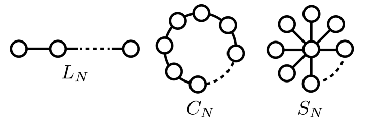
Figure 2: Depiction of the graphs used to illustrate the connectivities of the spin glass Hamiltonians in the considered examples.

III.1 $L_{N}$ connectivity

Figure 3: Performance of the VCQA solution in terms of the annealing time for 2 (blue with circles), 4 (orange with triangles), 7 (green with squares) and 10 (red with crosses) qubits for the $L_{N}$ connectivity. Panels (a) and (c) show the percentage error and fidelity of the solution, respectively, using two parameters per schedule functions (six in total). Panels (b) and (d) show the percentage error and fidelity, respectively, when employing the standard ramp schedule function.

As a first example we consider a spin chain with nearest-neighbour interaction, i.e. $L_{N}$ connectivity, described by

$$H_{L_{N}}=\sum_{j=1}^{N}\omega_{j}\sigma^{z}_{j}+\sum_{j=1}^{N-1}g_{j}\sigma^{z}_{j}\sigma^{z}_{j+1},$$ (10)

where $\omega_{j}$ and $g_{j}$ are randomly selected within the range $]0,1]$. Figure 3 (a) presents the average performance of our VCQA protocol over 100 random instances. We can see that the error of our solution falls below $1\%$ in a time less than $5\epsilon^{-1}$ for $N\leq 10$ qubits. In the case of superconducting circuits, $\epsilon$ is on the order of a few gigahertz, implying that our solution can be achieved in a span of a few nanoseconds. Figure 3 (b), shows the error for the same random cases using the ramp schedule function, which results in an error exceeding $15\%$ for the duration. We will highlight how close our result is to the real ground state by means of the fidelity $\mathcal{F}=|\langle\Phi_{0}|\psi_{T}\rangle|^{2}$. We remark that geometric distances do not serve as an effective cost function since they are challenging to measure experimentally and fail in degenerate cases. However, it is interesting to showcase them in numerical simulations and observe their correlation with the previously defined error.

Figures 3 (c) and (d) show the fidelity for both the VCQA protocol and a ramp schedule function, respectively. In all instances, the fidelity of the VCQA protocol exceeds 0.9. This is in strong contrast to the ramp schedule function, which can only achieve a fidelity greater than 0.85 for the case of two qubits, and a fidelity of less than 0.55 for ten qubits.

III.2 $C_{N}$ connectivity

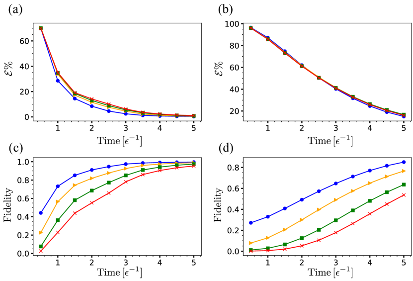
Figure 4: Performance of the VCQA solution in terms of the annealing time for 2 (blue with circles), 4 (orange with triangles), 7 (green with squares) and 10 (red with crosses) qubits for the $C_{N}$ connectivity. Panels (a) and (c) show the percentage error and fidelity of the solution, respectively, using two parameters per schedule functions (six in total). (b) and (d) show the percentage error and fidelity, respectively, when employing the standard ramp schedule function.

Now, we consider a one dimensional spin chain with periodic boundary conditions, i.e. $C_{N}$ connectivity, described by the Hamiltonian

$$H_{C_{N}}=\sum_{j=1}^{N}\omega_{j}\sigma^{z}_{j}+\sum_{j=1}^{N-1}g_{j}\sigma^{z}_{j}\sigma^{z}_{j+1}+g_{N}\sigma^{z}_{N}\sigma^{z}_{1}.$$ (11)

The Hamiltonians $H_{L_{N}}$ and $H_{C_{N}}$, differ only in their last term, specifically, the interaction between the first and last site of the chain. This additional term carries significant physical implications, being responsible for the frustration phenomena observed in antiferromagnetic rings with an odd number of sites. As in the previous case, $\omega_{j}$ and $g_{j}$ are randomly selected within the range $]0,1]$, and we consider the average behaviour over 100 random instances. Figure 4 displays the performance of our VCQA algorithm for the $C_{N}$ configuration. As depicted in Figure 4 (a) our results can achieve an error around $1\%$ within a time frame of approximately 5 $\epsilon^{-1}$. In contrast, the ramp schedule function strategy struggles to reduce the error below $15\%$, as can be seen in Figure 4 (b).

As depicted in Fig. 4 (c), we observe that all our results for up to 10 particles can achieve a fidelity greater than $0.9$, with values exceeding $0.98$ for up to four sites. In contrast, Figure 4 (d) reveals that the ramp schedule function fails to reach a fidelity of $0.85$ for the simple case of two sites, and for ten particles, the fidelity falls below $0.55$. This suggests that, similar to the previous case, our VCQA algorithm with only six parameters can yield good results within the coherence time of current quantum annealers for up to ten sites.

III.3 $S_{N}$ connectivity

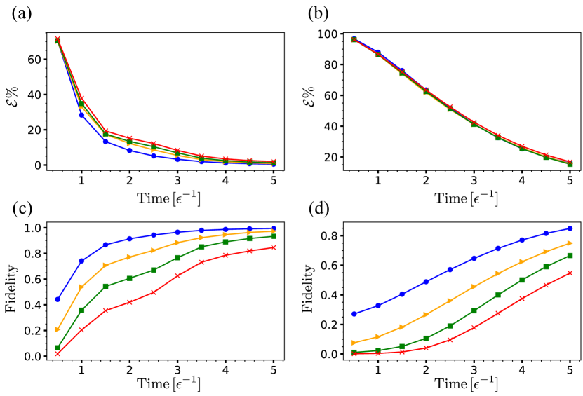
Figure 5: Performance of the VCQA solution in terms of the annealing time for 2 (blue with circles), 4 (orange with triangles), 7 (green with squares) and 10 (red with crosses) qubits for the $S_{N}$ connectivity. Panels (a) and (c) show the percentage error and fidelity of the solution, respectively, using two parameters per schedule functions (six in total). (b) and (d) show the percentage error and fidelity, respectively, when employing the standard ramp schedule function.

The last example that we use to test our VCQA algorithm is the $S_{N}$ connectivity, which means that one site is connected to all the others. This situation is described by

$$H_{S_{N}}=\sum_{j=1}^{N}\omega_{j}\sigma^{z}_{j}+\sigma^{z}_{1}\sum_{j=2}^{N}g_{j}\sigma^{z}_{j}.$$ (12)

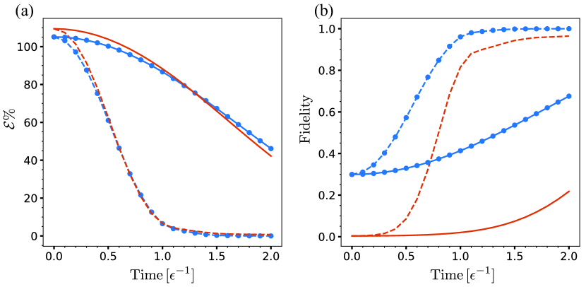
Figure 6: Performance of the VCQA solution in terms of the annealing time for 10 qubits for a Heisenberg chain with $y$-axis anisotropy given by Eq. (13).

This connectivity has the capacity to correlate all the sites through the central one, thereby increasing the multipartite quantum correlations within the system. This characteristic sets this system apart from the other examples, making it a valuable test case. Figure 5 shows the performance of our proposal for the $S_{N}$ case involving up to $10$ sites. Again, the local energies and couplings were selected randomly, where we used 100 instances and plotted the average performance.

As observed in Fig. 5 (a), the error attained in this case is slightly larger compared to the other connectivities. However, for 10 qubits, the error is less than $2\%$. In contrast, for the ramp schedule function strategy, depicted in Fig. 5 (b), the error for all cases exceeds $15\%$, even for the two qubit case, which in our scenario yields an error around $0.01\%$ in a time of $5\epsilon^{-1}$. It is important to underscore that we have used only six parameters in the algorithm, two per schedule function. This reflects the significant potential for precision that our algorithm could achieve if more parameters were employed in the optimization process.

Upon analyzing the fidelity that the solution can achieve, Fig. 5 (c) shows that in the worst case, i.e. $10$ qubits, the fidelity is slightly less than $0.85$, while the corresponding fidelity for the ramp strategy is less than $0.55$. For the simple case of two qubits, our VCQ algorithm achieves a fidelity around $0.99$ while the ramp strategy below $0.85$. These results once again demonstrate that for an $S_{N}$ connectivity, the VCQA proposal can attain accurate solutions in the coherence time of current quantum annealers.

IV Beyond spin-glass Hamiltonian

Although available quantum annealers do not allow for the implementation of non-stoquastic Hamiltonians, it is interesting to show the VCQA performance in presence of non-stoquastic terms. Figure 6 shows the case of a Heisenberg chain with $y$-axis anisotropy for ten and two qubits. Specifically, the final Hamiltonian corresponds to

$$H_{H}=\omega_{H}\sum_{j=1}^{N}\sigma^{z}_{j}+g_{H}\sum_{j=1}^{N-1}\left(\sigma_{j}^{x}\sigma_{j+1}^{x}+\delta\sigma_{j}^{y}\sigma_{j+1}^{y}+\sigma_{j}^{z}\sigma_{j+1}^{z}\right)\,,$$ (13)

with $\omega_{H}=\epsilon$, $g_{H}=0.1\epsilon$ and $\delta=5$. In Fig.  6, the dashed lines represent the results obtained with the VQCA method and the solid line with the ramp function. The dashed line with circles markers (blue) represent the performance for two qubits, while the dashed line without markers (red) for ten qubits. In the same way the solid line with circles markers (blue) represent the performance for two qubits, and the solid line without markers (red) for ten qubits. From Fig.  6 (a) we can see that the VCQA algorithm can reach an error less than $1\%$ in a time of $2\epsilon^{-1}$ for both, two and ten qubits. On the other side, for the usual ramp strategy, for the same time, the error is larger than $40\%$ even for the simple case of two qubits. If we observe Fig.  6 (b), we note that VCQA provides solutions with fidelity larger than $96\%$ and the ramp strategy cannot surpass the 0.7 for two qubits and 0.3 for then. It suggest that our VCQA protocol also has a great potential to reach fast an accurate solutions for non-stoquatic Hamiltonians.

Finally, for an annealing process, whose time evolution is governed by the Hamiltonian

$$H(t/T)=[1-g(t/T)]H_{i}+g(t/T)H_{f},$$ (14)

with $g(0)=0$ and $g(1)=1$, the annealing time is given by [46]

$$t_{f}=\frac{\langle H_{i}\rangle_{t_{f}}+\langle H_{f}\rangle_{0}-\langle H_{f}\rangle_{t_{f}}}{i\mathrm{Tr}(\bar{\rho}[H_{f},H_{i}])}.$$ (15)

Here, $\bar{\rho}$ is the time average of the density matrix during the evolution. This equation relates the final accuracy of the solution given by the final energy ($\langle H_{f}\rangle_{t_{f}}$) with the time needed for it. It is interesting to note that when we consider Hamiltonian evolutions governed by Eq. (1), the relation given by Eq. (15) for the annealing time changes to

$$t_{f}=\frac{\langle H_{i}\rangle_{t_{f}}+\langle H_{f}\rangle_{0}-\langle H_{f}\rangle_{t_{f}}+\mathcal{C}}{i\mathrm{Tr}(\bar{\rho}[H_{f},H_{i}])},$$ (16)

where

$$\mathcal{C}=\int_{0}^{t_{f}}\left[(\langle H_{f}\rangle-\langle H_{i}\rangle)\frac{d}{dt}\left(\frac{1}{F_{\Sigma}}\right)-\langle H_{aux}\rangle\frac{d}{dt}\left(\frac{\mathcal{R}_{31}}{F_{\Sigma}}\right)\right]dt\,.$$ (17)

Here, $F_{\Sigma}=F_{1}+F_{2}$ and $\mathcal{R}_{31}=F_{3}/F_{1}$, while a detailed derivation can be found in the appendix. We note that $\mathcal{C}=0$ for the case of the evolution of Eq. (14) since $F_{\Sigma}=1$ and $F_{3}=0$.

As the coefficient $\mathcal{C}$ depends on the shape of $F_{1}$, $F_{2}$, and $F_{3}$, which are arbitrary, it opens the door to get annealing evolutions with a reduced time $t_{f}$ for the same accuracy of $\langle H_{f}\rangle_{t_{f}}$. Nevertheless, a deep study about the behavior of this coefficient and its bounds is still needed.

V Conclusion

We have proposed the VCQA paradigm as a hybrid classical-quantum solution that strictly uses the available coherence time of current quantum annealers. Our approach hinges on two key aspects; the inclusion of an extra term in the Hamiltonian to expand the energy gap, and the utilization of three parametrized schedule functions. These functions are associated to the initial Hamiltonian, final Hamiltonian, and the auxiliary Hamiltonian. In particular, we consider $z$-local terms as our auxiliary Hamiltonian. This choice is advantageous as it is native to almost any physical platform, strongly contributing to the nontrivial enlargement of the energy gap.

We have tested our VCQA algorithm across three different connectivities; linear ($L_{N}$), cyclic ($C_{N}$) and star ($S_{N}$), up to 10 qubits. In all cases, we were able to achieve a solution error of less than $2\%$ within a time frame of $5\epsilon^{-1}$. This corresponds to a few nanoseconds for the current state-of-the-art in superconducting circuit technology, thereby outperforming the ramp schedule function strategy typically employed by quantum annealers. We remark that we have used only two parameters per schedule function in the optimization process. This demonstrates the significant potential for increased accuracy if we expand the number of optimization parameters.

We also show that this protocol can handle non-stoquastic Hamiltonians, as is the case of a Heisenberg chain. Even if current experiments may only tackle spin-glass models, it is interesting to show the performance of our VCQA proposal for a non-stoquastic case. Finally, when comparing our findings with a general annealing evolution without auxiliary term, we show that our protocol is able to reduce the annealing time for a given accuracy.

This work opens the door for a fully-coherent use of available quantum annealers, laying the path for leveraging quantum features to achieve faster and more accurate solutions.

Appendix A Annealing time

Let us consider the time evolution governed by the Hamiltonian

$$H(t)=F_{1}(t/T)H_{i}+F_{2}(t/T)H_{f}+F_{3}(t/T)H_{aux},$$ (18)

with $F_{1}(0)=F_{2}(1)=1$ and $F_{1}(1)=F_{2}(0)=F_{3}(0)=F_{3}(1)=0$. Then,

$$\frac{d}{dt}\langle H_{i}\rangle=iF_{2}\mathrm{Tr}(\rho[H_{f},H_{i}])+iF_{3}\mathrm{Tr}(\rho[H_{aux},H_{i}]),$$ (19)

$$\frac{d}{dt}\langle H_{f}\rangle=iF_{1}\mathrm{Tr}(\rho[H_{i},H_{f}])+iF_{3}\mathrm{Tr}(\rho[H_{aux},H_{f}]),$$ (20)

$$\frac{d}{dt}\langle H_{aux}\rangle=iF_{1}\mathrm{Tr}(\rho[H_{i},H_{aux}])+iF_{2}\mathrm{Tr}(\rho[H_{f},H_{aux}]).$$ (21)

If we consider that $[H_{f},H_{aux}]=0$, as in the cases of $z$-local auxiliary Hamiltonian for $H_{f}$ given by an spin glass one, we can write

$$\frac{d}{dt}\langle H_{i}\rangle-\frac{d}{dt}\langle H_{f}\rangle+\mathcal{R}_{31}\frac{d}{dt}\langle H_{aux}\rangle=iF_{\Sigma}\mathrm{Tr}(\rho[H_{f},H_{i}])$$

$$\Rightarrow i\mathrm{Tr}(\rho[H_{h},H_{i}])=\frac{1}{F_{\Sigma}}\frac{d}{dt}(\langle H_{i}\rangle-\langle H_{f}\rangle)+\frac{\mathcal{R}_{31}}{F_{\Sigma}}\frac{d}{dt}\langle H_{aux}\rangle\,.$$ (22)

Then, through integration, we obtain

$$it_{f}\mathrm{Tr}(\bar{\rho}[H_{h},H_{i}])=\left(\frac{\langle H_{i}\rangle-\langle H_{f}\rangle}{F_{\Sigma}}\right)\Bigg{|}_{0}^{t_{f}}+\frac{\mathcal{R}_{31}\langle H_{aux}\rangle}{F_{\Sigma}}\Bigg{|}_{0}^{t_{f}}+\int_{0}^{t_{f}}\left[(\langle H_{f}\rangle-\langle H_{i}\rangle)\frac{d}{dt}\left(\frac{1}{F_{\Sigma}}\right)-\langle H_{aux}\rangle\frac{d}{dt}\left(\frac{\mathcal{R}_{31}}{F_{\Sigma}}\right)\right]dt,$$ (23)

where $\bar{\rho}=\frac{1}{t_{f}}\int_{0}^{t_{f}}\rho dt$. Using the boundary conditions for the functions $F_{1}$, $F_{2}$ and $F_{3}$, we obtain

$$t_{f}=\frac{\langle H_{i}\rangle_{t_{f}}+\langle H_{f}\rangle_{0}-\langle H_{f}\rangle_{t_{f}}+\mathcal{C}}{i\mathrm{Tr}(\bar{\rho}[H_{f},H_{i}])}\,,$$ (24)

with

$$\mathcal{C}=\int_{0}^{t_{f}}\left[(\langle H_{f}\rangle-\langle H_{i}\rangle)\frac{d}{dt}\left(\frac{1}{F_{\Sigma}}\right)-\langle H_{aux}\rangle\frac{d}{dt}\left(\frac{\mathcal{R}_{31}}{F_{\Sigma}}\right)\right]dt\,.$$ (25)

References

- [1] T. Albash and D. A. Lidar, Adiabatic quantum computation, Rev. Mod. Phys. 90, 015002 (2018).
- [2] A. M. Childs, E. Farhi, and J. Preskill, Robustness of adiabatic quantum computation, Phys. Rev. A 65, 012322 (2001).
- [3] M. S. Sarandy and D. A. Lidar, Adiabatic Quantum Computation in Open Systems, Phys. Rev. Lett. 95, 250503 (2005).
- [4] M. B. Hastings, The Power of Adiabatic Quantum Computation with No Sign Problem, Quantum 5, 597 (2021).
- [5] S. Boixo et al., Computational multiqubit tunnelling in programmable quantum annealers, Nat. Commun. 7, 10327 (2016).
- [6] L. Buffoni and M. Campisi, Thermodynamics of a quantum annealer, Quantum Sci. Technol. 5, 035013 (2020).
- [7] R. Hamerly et al., Experimental investigation of performance differences between coherent Ising machines and a quantum annealer, Sci. Adv. 5, eaau0823 (2019).
- [8] T. Lanting et al., Entanglement in a Quantum Annealing Processor, Phys. Rev. X 4, 021041 (2014).
- [9] T. Albash, I. Hen, F. M. Spedalieri, and D. A. Lidar, Reexamination of the evidence for entanglement in a quantum annealer, Phys. Rev. A 92, 062328 (2015).
- [10] P. Hauke, H. G. Katzgraber, and W. Lechner, Perspectives of quantum annealing: methods and implementations, Rep. Prog. Phys. 83, 054401 (2020).
- [11] E. J. Crosson and D. A. Lidar, Prospects for quantum enhancement with diabatic quantum annealing, Nat. Rev. Phys. 3, 466 (2021).
- [12] D. Aharonov, W. van Dam, J. Kempe, Z. Landau, S. Lloyd, and O. Regev, Adiabatic Quantum Computation Is Equivalent to Standard Quantum Computation, SIAM Rev. 50, 755 (2008).
- [13] S. H. W. van der Ploeg et al., Adiabatic Quantum Computation With Flux Qubits, First Experimental Results, IEEE Trans. Appl. Supercond. 17, 113 (2007).
- [14] I. Ozfidan et al., Demonstration of a Nonstoquastic Hamiltonian in Coupled Superconducting Flux Qubits, Phys. Rev. Appl. 13, 034037 (2020).
- [15] J. Du, N. Xu, X. Peng, P. Wang, S. Wu, and D. Lu, NMR Implementation of a Molecular Hydrogen Quantum Simulation with Adiabatic State Preparation, Phys. Rev. Lett. 104, 030502 (2010).
- [16] X. Peng, Z. Liao, N. Xu, G. Qin, X. Zhou, D. Suter, and J. Du, Quantum Adiabatic Algorithm for Factorization and Its Experimental Implementation, Phys. Rev. Lett. 101, 220405 (2008).
- [17] A. W. Glaetzle, R. M. W. van Bijnen, P. Zoller, and W. Lechner, A coherent quantum annealer with Rydberg atoms, Nat. Commun. 8, 15813 (2017).
- [18] Y. Luo and X. Li, Effect of Quantum Statistics on Computational Power of Atomic Quantum Annealers, arXiv: 2209.00201 [quant-ph] (2022).
- [19] D. Willsch, M Willsch, C. D. Gonzalez Calaza, F. Jing, H. De Raedt, M. Svensson, and K. Michielsen. Benchmarking Advantage and D-Wave 2000Q quantum annealers with exact cover problems, Quantum Inf. Process. 21, 141 (2022).
- [20] R. Orús, S. Mugel, and E. Lizaso, Forecasting financial crashes with quantum computing, Phys. Rev. A 99, 060301 (2019).
- [21] Y. Ding, J. Gonzalez-Conde, L. Lamata, J. D. Martín-Guerrero, E. Lizaso, S. Mugel, X. Chen, R. Orús, E. Solano, and M. Sanz, Towards Prediction of Financial Crashes with a D-Wave Quantum Computer, Entropy 25, 323 (2023).
- [22] T. Gabor, M. L. Rosenfeld, S. Feld, and C. Linnhoff-Popien, How to Approximate any Objective Function via Quadratic Unconstrained Binary Optimization, arXiv:2204.11035 [quant-ph] (2022).
- [23] F. Glover, G. Kochenberg, and Y. Du, A Tutorial on Formulating and Using QUBO Models, arXiv:1811.11538 [cs.DS] (2019).
- [24] N. Chancellor, S. Zohren, and P. A. Warburton, Circuit design for multi-body interactions in superconducting quantum annealing systems with applications to a scalable architecture, npj Quantum Inf. 3, 21 (2017).
- [25] J. Cohen, A. Khan, and C. Alexander, Portfolio Optimization of 40 Stocks Using the DWave Quantum Annealer, arXiv:2007.01430 [q-fin.GN] (2020).
- [26] G. Rosenberg, P. Haghnegahdar, P. Goddard, P. Carr, K. Wu, and M. López de Prado, Solving the Optimal Trading Trajectory Problem Using a Quantum Annealer, IEEE J. Sel. Top. Signal Process. 10, 1053 (2016).
- [27] M. Streif, F. Neukart, and M. Leib, Solving quantum chemistry problems with a d-wave quantum annealer, in International Workshop on Quantum Technology and Optimization Problems (Springer, New York, 2019), pp. 111–122.
- [28] R. Babbush, P. J. Love, and A. Aspuru-Guzik, Adiabatic Quantum Simulation of Quantum Chemistry, Sci. Rep. 4, 6603 (2014).
- [29] A. Teplukhin, B. K. Kendrick, S. Tretiak, and P. A. Dub, Adiabatic Quantum Simulation of Quantum Chemistry, Sci. Rep. 4, 6603 (2014).
- [30] V. Dixit, R. Selvarajan, M. A. Alam, T. S. Humble, and S. Kais, Training and Classification using a Restricted Boltzmann Machine on the D-Wave 2000Q, arXiv:2005.03247 [cs.LG] (2020).
- [31] D. Willsch, M. Willsch, H. De Raedt, and K. Michielsen, Support vector machines on the D-Wave quantum annealer, Comput. Phys. Commun. 248, 107006 (2020).
- [32] R. K. Nath, H. Thapliyal, and T. S. Humble, A Review of Machine Learning Classification Using Quantum Annealing for Real-World Applications, SN Comp. Sci. 2, 365 (2021).
- [33] S. Yarkoni, E. Raponi, S. Schmitt, and T. Bäck, Quantum Annealing for Industry Applications: Introduction and Review, arXiv:2112.07491 [quant-ph] (2021).
- [34] M. H. Amin, Searching for quantum speedup in quasistatic quantum annealers, Phys. Rev. A 92, 052323 (2015).
- [35] A. S. Koshikawa, M. Ohzeki, T. Kadowaki, and K. Tanaka, Benchmark Test of Black-box Optimization Using D-Wave Quantum Annealer, J. Phys. Soc. Jpn. 90, 064001 (2021).
- [36] L. Zeng, J. Zhang, and M. Sarovar, Schedule path optimization for adiabatic quantum computing and optimization, J. Phys. A: Math. Theor. 49, 165305 (2016).
- [37] A. T. Rezakhani, W.-J. Kuo, A. Hamma, D. A. Lidar, and P. Zanardi, Quantum Adiabatic Brachistochrone, Phys. Rev. Lett. 103, 080502 (2009).
- [38] C. Brif, M. D. Grace, M. Sarovar, and K. C. Young, Exploring adiabatic quantum trajectories via optimal control, New J. Phys. 16, 065013 (2014).
- [39] M. Hofmann and G. Schaller, Probing nonlinear adiabatic paths with a universal integrator, Phys. Rev. A 89, 032308 (2014).
- [40] E. Farhi, J. Goldstone, and S. Gutmann, Quantum Adiabatic Evolution Algorithms with Different Paths, arXiv:quant-ph/0208135 (2002).
- [41] A. Perdomo-Ortiz, S. E. Venegas-Andraca, and A. Aspuru-Guzik, A study of heuristic guesses for adiabatic quantum computation, Quantum Inf. Process. 10, 33 (2011).
- [42] E. Crosson, E. Farhi, C. Y.-Y. Lin, H.-H. Lin, and P. Shor, Different Strategies for Optimization Using the Quantum Adiabatic Algorithm, arXiv:1401.7320 [quant-ph] (2014).
- [43] X, Yang, R. Liu, J. Li, and X. Peng, Optimizing adiabatic quantum pathways via a learning algorithm, Phys. Rev. A 102, 012614 (2020).
- [44] N. Barraza, G. A. Barrios, J. Peng, L. Lamata, E. Solano, and F. Albarrán-Arriagada. Analog quantum approximate optimization algorithm. Quantum Sci. Technol. 7, 045035 (2022)
- [45] F. N. Fritsch and J. Butland. A Method for constructing local monotone piecewise cubic interpolants. SIAM J. Sci. Stat. Comput. 5, 300 (1984)
- [46] L. P. García-Pintos, L. T. Brady, J. Bringewatt, and Y.-K. Liu. Lower Bounds on Quantum Annealing Times. Phys. Rev. Lett. 130, 140601 (2023)