Optimum Monitoring of Heterogeneous
Continuous Time Markov Chains

Abstract

We study a remote monitoring system in which a collection of ergodic, aperiodic, mutually independent, and heterogeneous continuous time Markov chain (CTMC) based information sources is considered. In this system, a common remote monitor samples the states of the individual CTMCs according to a Poisson process with possibly different per-source sampling rates, in order to maintain remote estimates of the states of each of the sources. Three information freshness models are considered to quantify the accuracy of the remote estimates: fresh when equal (FWE), fresh when sampled (FWS) and fresh when close (FWC). For each of these freshness models, closed-form expressions are derived for mean information freshness for a given source. Using these expressions, optimum sampling rates for all sources are obtained so as to maximize the weighted sum freshness of the monitoring system under an overall sampling rate constraint. This optimization problem possesses a water-filling solution with quadratic worst case computational complexity in the number of information sources. Numerical examples are provided to validate the effectiveness of the optimum sampler in comparison to several baseline sampling policies.

I Introduction

Timely delivery of status packets from a number of information sources for maintaining information freshness at a remote monitoring point has recently gained significant attention for the development of applications requiring real-time monitoring and control. A recently introduced commonly used process is age of information (AoI) which is a continuous-valued continuous-time stochastic process maintained at the remote monitor (destination) that keeps track of the time elapsed since the reception of the last status packet received from a particular information source. The AoI process was first introduced in [1] for a single-source M/M/1 queuing model which resulted in substantial interest in the modeling of AoI and its optimization in very general settings including multiple sources [2, 3]. In the majority of existing work, the mean AoI is used as the information freshness metric, whereas, to a lesser extent, higher order moments or tail distribution, of the AoI process, have also been employed as freshness metrics. The continuous-valued, discrete-time peak AoI (PAoI) process which is obtained by sampling the AoI process at pre-reception instants, has also gained the attention due to its relative simplicity and amenability to analytical modeling and optimization [4, 5]. On the other hand, various works focused on the discrete-time variation of the AoI process [6, 7].

In the general AoI setting, information sources generate status update packets that contain the samples of an underlying random process, e.g., a sensor sampling a physical quantity such as temperature, humidity, etc., or an information item with time-varying content such as news, weather reports, etc., which are subsequently delivered to the destination through a communication network. In the push-based communication paradigm, information sources decide when to sample and form the information packets, which are subsequently forwarded towards the destination [8, 9, 10]. On the other hand, in pull-based communications, monitors proactively send requests to the information sources upon which sampling takes place [11, 12]. As an example, pull-based systems are common in Web crawlers which manage local copies of remote Web pages for Web search engines [13].

In this paper, the interest will be on the remote estimation (at the destination) of discrete-valued information sources for which the status of the sources change at random instants. In particular, we will focus on a heterogeneous set of finite, ergodic, and aperiodic CTMC based information sources for which the average rate at which state changes take place, will be different among the sources in the set. Although performance metrics derived from AoI and PAoI processes have been extremely useful for the development of status update systems for continuous-valued random processes, these metrics do not take into consideration the statistical characterization of the underlying random processes. A key feature of the AoI process is that it increases with unit slope between two packet reception instants, irrespective of how many state changes have taken place at the source in this interval.

Therefore, there is a need for using information freshness metrics that are suitable for the remote estimation of discrete-valued random processes with a-priori known statistical characterization. In some applications including cache update systems, the information at the destination may not hold a value unless the content at the destination is synchronized with the source. In this case, binary freshness process is suitable which takes the value of one when the information at the destination is up to date (or is in sync with the source), and is zero otherwise [14, 15, 16, 17, 13]. Alternatively, the non-binary version age process keeps track of the number of status changes that have occurred at the source since the last time the content at the destination is de-synchronized with the source [18, 19, 20, 21]. While binary freshness and version age processes do not take into account the elapsed time, the age of synchronization (AoS) process defined as the elapsed time since the content at the destination has become de-synchronized with the source, presents an alternative metric that combines binary freshness and AoI [22, 23, 24].

Figure 1: Remote monitoring system for which the monitor samples the CTMC $X_{n}(t)$ associated with source-$n$ with intensity $\lambda_{n}$ to maintain an estimate $\tilde{X}_{n}(t)$ of $X_{n}(t)$.

In this paper, we consider the pull-based communication system in Fig. 1 in which $N$ CTMC based information sources, denoted by $X_{n}(t)$, $t\geq 0$, are sampled by a common remote monitor according to a Poisson process with intensity $\lambda_{n}$ to maintain a martingale estimate $\tilde{X}(t)$, $t\geq 0$, of the original processes. The martingale estimate for the state of the CTMC $X_{n}(t)$ at a future epoch, given the current and preceding observed states, is the current observed state. Such an estimator is known to be optimum in the mean square sense for martingale processes; see [25]. However, CTMCs are not martingale processes, and hence more sophisticated estimators for CTMCs including the maximum likelihood (MLE) or minimum mean square error (MMSE) estimators, can also be used, but at the expense of increased computational complexity in deriving the expressions for the freshness metrics and subsequently obtaining the optimum sampler. The focus of this paper is the use of martingale estimators for CTMCs which are relatively simple to implement and which give rise to closed-form expressions for mean freshness metrics, which is crucial for the applicability of convex optimization techniques.

We propose three freshness models to quantify the accuracy of the martingale estimators. In the fresh when equal (FWE) binary freshness model, the information is fresh at the destination when the remote estimator is in sync with the state of the original source. In the fresh when sampled (FWS) freshness model (which is also binary), the information becomes stale when the state of the original source changes and it becomes fresh only when a new sample is taken. Although the FWE model is more realistic, closed-form expressions amenable to optimization will be shown to be readily available for the FWS model for a more general class of CTMCs, than the FWE model. The non-binary fresh when close (FWC) model is a generalization of FWE, where the level of freshness depends on the proximity of the original process and its estimator at the monitor, yielding more flexibility than FWE.

In this work, for these three freshness models, we find the optimum sampling rate for each source that maximizes a weighted sum freshness for the system, under a total sampling rate constraint for the monitor. We show that this optimization problem possesses a water-filling structure which amounts to a procedure in which a limited volume of water is poured into a pool organized into a number of bins with different ground levels with the water level in each bin giving the desired optimum solution [26]. Water-filling based optimization has been successfully used in solving optimal resource allocation problems arising in wireless networks; see [27, 26] for two surveys on water-filling based optimization for wireless networks, and examples [28] and [29], for a power allocation problem for a wireless network and energy allocation problem for energy harvesting transmitters, respectively. Iterative methods are available for water-filling based optimization which will be shown to give rise to an algorithm for the optimum monitoring problem in Fig. 1 with quadratic worst-case computational complexity in the number of sources.

The contributions of our paper are as follows: 1) To the best of our knowledge, optimum sampling of heterogeneous CTMCs under overall sampling rate constraints has not been explored in the literature. Our work initiates this line of study. 2) We derive closed-form expressions for mean freshness for FWE, FWC, and FWS models for finite, ergodic, and aperiodic CTMCs. For the FWS model, the obtained expression is in terms of the sum of first order rational functions of the sampling rate which is a strictly concave increasing function. For the FWE and FWC models, similar expressions are obtained for the sub-case of time-reversible CTMCs (using the real-valued eigenvalues, and eigenvectors of the corresponding generators) that cover the well-established birth-death Markov chains that arise frequently in the performance of computer and communication systems. 3) The obtained expressions allow us to use computationally efficient water-filling algorithms and obtain optimum sampling policies.

The remainder of this paper is organized as follows. Related work is summarized in Section II. In Section III, the detailed system model is presented. Section IV addresses the derivation of mean freshness expressions for the FWE, FWC, and FWS models. The water-filling based optimization algorithm is presented in Section V. A comparative evaluation of the proposed optimum sampler and several baseline sampling policies are presented in Section VI. Conclusions, some open problems and potential future directions are given in Section VII.

II Related Work

The remote estimation problem of information sources is studied in various works. In [30], the authors study the remote estimation of a linear time-invariant dynamic system while focusing on the trade-off between reliability and freshness. The reference [31] investigates the problem of sampling a Wiener process with samples forwarded to a remote estimator over a channel that is modeled as a queue. The authors of [32] study a transmitter monitoring the evolution of a two-state discrete Markov source and sending status updates to a destination over an unreliable wireless channel for the purpose of real-time source reconstruction for remote actuation. This work is then extended in [33] with more general discrete stochastic source processes and resource constraints. The work presented in [34] studies the trade-off between the sampling frequency and staleness in detecting the events through a freshness metric called age penalty which is defined as the time elapsed since the first transition out of the most recently observed state. The authors of [35] investigate the effect of AoI on the accuracy of a remote monitoring system which displays the latest state information from a continuous-time Markov chain and they develop a computational method for finding the conditional probability of the displayed state, given the actual current state of the information source. A common feature of the above works is the existence of a single information source which gets to be sampled. On the other hand, reference [36] studies the sampling of a collection of heterogeneous two-state CTMC-based information sources each modeling whether an individual is infected with a virus or not while using the binary freshness metric, and reference [20] studies sampling of multiple heterogeneous Poisson processes representing the citation indices of multiple researchers with the goal of keeping timely estimates (similar to version age) of all the random processes. In the current manuscript, we study a heterogeneous collection of general finite-state (not necessarily two-state) CTMC-based information sources with three different freshness models (including the binary freshness metric) where the sources need to be sampled for remote estimation with a constraint on the overall sampling rate.

III System Model

We consider the monitoring system in Fig. 1 with $N$ continuous-time information sources each of which is a finite-dimensional, ergodic, and aperiodic CTMC. The CTMC associated with source-$n$ is denoted by $X_{n}(t)$, $n\in\mathcal{N}=\{1,2,\ldots,N\}$, $t\geq 0$, and $X_{n}(t)\in\{1,2,\ldots,K_{n}\}$, where $K_{n}$ is the size of state space for $X_{n}(t)$. The process $X_{n}(t)$ has the infinitesimal generator $Q_{n}$ of size $K_{n}$ with its $(i,j)$th entry denoted by $q_{n,ij}$ which is the transition rate from state $i$ to state $j$ for $i\neq j$ and its diagonal entries are strictly negative satisfying $Q_{n}e=0$, where $e$ is a column vector of ones of appropriate size. From Perron-Frobenius theory, $Q_{n}$ has a left eigenvector $\pi_{n}$ and right eigenvector $e$, associated with the simple eigenvalue of zero and all other eigenvalues having strictly negative real parts. The $i$th element of the steady-state vector $\pi_{n}$ is denoted by $\pi_{n,i}$ which is the steady-state probability of the process $X_{n}(t)$ being in state $i$, i.e., $\pi_{n,i}=\lim_{t\rightarrow\infty}\mathbb{P}[X_{n}(t)=i]$. The steady-state vector satisfies $\pi_{n}Q_{n}=0$ and $\pi_{n}e=1$. The transition rate out of state $i$ is denoted by $\sigma_{n,i}=\sum_{j\neq i}q_{n,ij}$. The average transition intensity of source-$n$ is denoted by $r_{n}$, i.e., $r_{n}=\sum_{i=1}^{K_{n}}\pi_{n,i}\sigma_{n,i}$ which is the long-term frequency of state transitions for the CTMC $X_{n}(t)$. Intuitively, sources with larger transition intensities need to be sampled at higher sampling rates for keeping the information fresh at the remote monitor; in this paper, we will determine exactly how often each source should be sampled relative to others, depending on the given system parameters. We denote by $r$ the system transition intensity, $r=\sum_{i=1}^{N}r_{n}$.

The remote monitor in Fig. 1 samples the original process $X_{n}(t)$ according to a Poisson process with intensity $\lambda_{n}>0$ in order to maintain an estimate of the instantaneous state of the original information process. In this paper, we propose to use the martingale estimator $\tilde{X}_{n}(t)$ which is given as $\tilde{X}_{n}(t)=X_{n}(t^{\prime})$, where $t^{\prime}$ is the latest sampling time before $t$. The martingale estimator is very simple to maintain, and moreover, we will show that it is possible to obtain closed-form expressions for the performance of martingale estimators for time-reversible CTMCs, which subsequently leads to an algorithmic optimization procedure for obtaining the sampling rates in a heterogeneous setting.

The accuracy of the remote estimator is studied with three information freshness models described below. For the FWE information freshness model, the information is said to be fresh at the remote monitor only when the original process and its estimate are equal, i.e., $\tilde{X}_{n}(t)=X_{n}(t)$, and is otherwise stale. In the FWE model, there is no value at all in a sample, unless the original process and its estimator are synchronized. Hence, the binary freshness process $F_{n,e}(t)$ is defined as $F_{n,e}(t)=1$ when $\tilde{X}_{n}(t)=X_{n}(t)$, and $F_{n,e}(t)=0$ otherwise. The mean freshness metric for FWE is given by

$$\mathbb{E}[F_{n,e}(t)] =\lim_{\tau\rightarrow\infty}\frac{1}{\tau}\int_{0}^{\tau}F_{n,e}(t)\differential{t},$$ (1)

for quantifying the accuracy of the remote estimator.

Figure 2: Sample paths of the processes $X(t)$, $\tilde{X}(t)$, $F_{e}(t)$, $F_{c}(t)$ and $F_{s}(t)$ for a source with 3 states for an example scenario.

In the FWC model, we assume that there may be a value in a sample when the original process and its estimator are close enough to each other despite being out of sync, from a certain semantic perspective. For this purpose, for FWC, we introduce a proximity matrix $P_{n}=\{p_{n,ij}\}$, $0\leq p_{n,ij}\leq 1$ for source-$n$, and subsequently define a non-binary freshness process $F_{n,c}(t)$ which takes the value $p_{n,ij}$ when $X_{n}(t)=i$ and $\tilde{X}_{n}(t)=j$. In particular, $p_{n,ii}=1$, representing perfect freshness when the original process and its estimator are synchronized. Close to unity values of $p_{n,ij}$ are representative of proximity between the states $i$ and $j$. When $P_{n}$ is taken as the identity matrix, FWC reduces to FWE. To motivate FWC, consider a CTMC whose states is the number of busy servers in a server farm. The task of the remote monitor is to maintain an accurate estimate of the number of busy servers for the purpose of shutting down some of the idle servers for energy efficiency purposes. For this application, FWC may provide a more flexible model than FWE since energy can still be saved when the two processes of interest are close to each other even when they are not in perfect sync.

For the FWS model, the binary freshness process $F_{n,s}(t)$ is set whenever the process is sampled, and it stays set until $X_{n}(t)$ makes a transition at which instant $F_{n,s}(t)$ becomes zero. For FWS, when the freshness process is stale, it cannot be set until the remote monitor re-samples the process, which is in contrast with FWE. The advantage of the FWS model is that it represents certain applications where freshness can be regained only with an explicit user action once it has been lost, and further, closed from expressions can be obtained for FWS for a very general class of CTMCs making it suitable for convex optimization in these general cases.

The mean freshness metrics $\mathbb{E}[F_{n,c}(t)]$ and $\mathbb{E}[F_{n,s}(t)]$ for the FWC and FWS models, respectively, are defined similar to (1). When the index of the source is immaterial, the subscript $n$ is dropped as for the source process $X(t)$ and its estimator $\tilde{X}(t)$ along with the corresponding freshness processes $F_{e}(t)$, $F_{c}(t)$, and $F_{s}(t)$ for FWE, FWC, and FWS, respectively.

Fig. 2 depicts the sample paths of the processes $X(t)$, $\tilde{X}(t)$, $F_{e}(t)$, $F_{c}(t)$ and $F_{s}(t)$ for a source with three states $\{1,2,3\}$ for an example scenario where the proximity matrix $P$ for FWC is chosen such that $p_{ij}=1$ when $|i-j|=0$, $p_{ij}=0.5$ when $|i-j|=1$, and $p_{ij}=0$ when $|i-j|=2$. Note that when $F_{s}(t)=1$, then $F_{e}(t)=1$, but not otherwise. Therefore, $\mathbb{E}[F_{e}(t)]\geq\mathbb{E}[F_{s}(t)]$ for any choice of the sampling rate $\lambda$. Moreover, $\mathbb{E}[F_{c}(t)]\geq\mathbb{E}[F_{e}(t)]$ since $F_{c}(t)$ can be larger than zero when $F_{e}(t)=0$, stemming from the structure of the proximity matrix $P$. Thus, $\mathbb{E}[F_{c}(t)]\geq\mathbb{E}[F_{e}(t)]\geq\mathbb{E}[F_{s}(t)]$.

IV Analytical Expressions for Mean Freshness

The subscript $n$ indicating the source index is dropped for convenience in the current section where the mean freshness is derived for a single ergodic, aperiodic CTMC $X(t)$ for the three freshness models FWE, FWC, and FWS.

IV-A FWE Model

Theorem 1 provides an expression for $f(\lambda)=\mathbb{E}[F_{e}(t)]$ for the FWE model for the CTMC $X(t)$.

Theorem 1.

Let the ergodic and aperiodic CTMC $X(t)\in\{1,2,\ldots,K\}$ with generator $Q$ and steady-state vector $\pi$ be Poisson sampled with sampling rate $\lambda$. Then, for the FWE model, the mean freshness $f(\lambda)=\mathbb{E}[F_{e}(t)]$ is given by,

$$f(\lambda) =\lambda\pi{\rm diag}[(\lambda I-Q)^{-1}],$$ (2)

where ${\rm diag}[\cdot]$ represents a column vector composed of the diagonal entries of its matrix argument.

Proof.

Let us consider the two-dimensional random process $Y(t)=(\tilde{X}(t),X(t))$, which is also Markov. To see this, note that, the transition intensity from state $(i,j)$ to $(i,j^{\prime})$ is $q_{jj^{\prime}}$ and from state $(i,j)$ to $(j,j)$ for $j\neq i$ is $\lambda$. Let the steady-state vector of the process $Y(t)$ be denoted by $y$, i.e., $y_{ij}=\lim_{t\rightarrow\infty}\mathbb{P}[Y(t)=(i,j)]$, $1\leq i,j\leq K$. Let $Y$ be a $K\times K$ matrix such that $Y=\{y_{ij}\}$. The global balance equations (GBE) for CTMCs are a set of equations, one for each state $s$ of the CTMC, which states that the total probability flux out of a state $s$ should be equal to the total probability flux from other states into the state $s$, in steady-state. Applying the GBE for the state $(i,i)$ of $Y(t)$ provides the following equation for each $i$, $1\leq i\leq K$,

$$y_{ii}\sigma_{i} =\sum_{j\neq i}y_{ij}q_{ji}+\sum_{j\neq i}y_{ji}\lambda,$$ (3)

$$=\sum_{j\neq i}y_{ij}q_{ji}+\lambda(\pi_{i}-y_{ii}),$$ (4)

where the last equality stems from the identity $\pi_{i}=\sum_{j}y_{ji}$. On the other hand, when the GBE is applied for the state $(i,k)$, $k\neq i$, then we obtain the following,

$$y_{ik}(\sigma_{k}+\lambda)=\sum_{j\neq k}y_{ij}q_{jk},\quad 1\leq i\leq K,\ k\neq i.$$ (5)

Writing the equations (4) and (5) in a matrix form, we obtain for each $i$, $1\leq i\leq K$,

$$Y(i,:)(Q-\lambda I) =-\lambda\pi_{i}I(i,:),$$ (6)

where $Y(i,:)$ and $I(i,:)$ denote the $i$th row of $Y$ and the $i$th row of the identity matrix, respectively. In FWE, the freshness process $F_{e}(t)=1$ when the joint process $Y(t)$ is visiting state $(i,i)$ for some state $i$ and $F_{e}(t)=0$ otherwise. Therefore,

$$\mathbb{E}[F_{e}] =\sum_{i=1}^{K}y_{ii},$$ (7)

which yields the identity (2). ∎

We now shift our focus to the special case of time-reversible CTMCs which subsume birth-death CTMCs as a subcase, for which it is not only possible to simplify but also to show the strict concavity of the expression in (2) with respect to the variable $\lambda$. Recall that a time-reversible CTMC has a generator $Q$ which satisfies [37],

$$\pi_{i}q_{ij} =\pi_{j}q_{ji},\quad i\neq j.$$ (8)

Let

$$\Pi= {\rm diag}\{\pi_{1},\pi_{2},\ldots,\pi_{K}\},$$ (9)

be the diagonal matrix composed of the entries of $\pi$. Also let

$$S =\Pi^{1/2}Q\Pi^{-1/2},$$ (10)

which is a symmetric matrix from (8). Symmetric matrices have real eigenvalues and they are diagonalizable by orthogonal transformations. Therefore, there exists an orthonormal matrix $U$ such that

$$U^{T}SU =D={\rm diag}\{-d_{1},-d_{2},\ldots,-d_{K-1},0\},$$ (11)

where $-d_{i}$, with $d_{i}>0$, are the corresponding real eigenvalues of the matrix $S$. Moreover, the matrix defined by $T=\Pi^{-1/2}U$ diagonalizes the original generator $Q$, i.e.,

$$T^{-1}QT =D,$$ (12)

and the eigenvalues of $T$ being the same as those of $S$.

Let the $(i,j)$th entries of $T$ and $\tilde{T}=T^{-1}$ be denoted by $t_{ij}$ and $\tilde{t}_{ij}$, respectively. The way the transformation matrix $T$ is defined, the $i$th row of ${\tilde{T}}$, i.e., the $i$th left eigenvector of $Q$, is obtained by post-multiplying by $\Pi$ the transpose of the $i$th column of $T$, i.e., the transpose of the $i$th right eigenvector of $Q$. Moreover, the row vector $\pi$ is the $K$th row of $\tilde{T}$ and $e$ is the $K$th column of $T$ in (12).

The following theorem gives a simplified expression for the mean freshness in terms of the sum of first-order rational functions of the variable $\lambda$ for time-reversible CTMCs.

Theorem 2.

Consider the process $X(t)$ of Theorem 1 with generator $Q$ which is time-reversible and with diagonalizing transformation matrix $T$ as given in (12). Then, the mean freshness $f(\lambda)=\mathbb{E}[F_{e}(t)]$ is given for the FWE model by

$$f(\lambda) =\sum_{j=1}^{K}\pi_{j}^{2}+\lambda\sum_{j=1}^{K-1}\frac{b_{j}}{\lambda+d_{j}},$$ (13)

$$=1-\sum_{j=1}^{K-1}\frac{a_{j}}{\lambda+d_{j}},$$ (14)

where $a_{j}$ and $b_{j}$, for $1\leq j\leq K-1$, are given by

$$b_{j} =\sum_{i=1}^{K}{\pi}_{i}^{2}t_{ij}^{2}=\sum_{i=1}^{K}{\tilde{t}_{ji}^{2}},\quad a_{j}=b_{j}d_{j}.$$ (15)

Moreover, $f(\lambda)$ is increasing and strictly concave, and has a continuous derivative $f^{\prime}(\lambda)$ with $\lim_{\lambda\rightarrow 0^{+}}f(\lambda)=\sum_{j=1}^{K}\pi_{j}^{2}$.

Proof.

Using the diagonalization equation (12), we first write the term $A=(\lambda I-Q)^{-1}=T(\lambda I-D)^{-1}T$ appearing in (2) as follows,

$$A =T\matrixquantity(\frac{1}{\lambda+d_{1}}&&&\\ &\ddots&&\\ &&\frac{1}{\lambda+d_{K-1}}&\\ &&&\frac{1}{\lambda})T^{-1}.$$ (16)

Using (2) and (16), we have

$$\frac{f(\lambda)}{\lambda} =\sum_{i=1}^{K}{\pi}_{i}A_{ii},$$ (17)

$$=\sum_{i=1}^{K}{\pi}_{i}\sum_{j=1}^{K}t_{ij}\tilde{t}_{ji}\frac{1}{\lambda+d_{j}},$$ (18)

$$=\sum_{j=1}^{K-1}\underbrace{\sum_{i=1}^{K}{\pi}_{i}^{2}t_{ij}^{2}}_{b_{j}}\frac{1}{\lambda+d_{j}}+\frac{1}{\lambda}\sum_{i=1}^{K}\pi_{i}^{2},$$ (19)

$$=\sum_{j=1}^{K-1}\frac{b_{j}}{\lambda+d_{j}}+\frac{1}{\lambda}\sum_{i=1}^{K}\pi_{i}^{2},$$ (20)

since $\tilde{t}_{ji}=\pi_{i}t_{ij}$ and also $\sum_{i=1}^{K}{\pi}_{i}t_{iK}\tilde{t}_{Ki}=\sum_{i=1}^{K}\pi_{i}^{2}$ by observing that $t_{iK}=1$ and $\tilde{t}_{Ki}={\pi}_{i}$. The result in (20) gives the desired expression in (13). Then, (14) follows directly from (20) and also the fact that $\lim_{\lambda\rightarrow\infty}f(\lambda)=1$.

Moreover, the coefficients $a_{j}$ and $b_{j}$ are strictly positive since $\pi_{i}>0$ and the entries of a column of $T$ cannot be all zero. A first-order rational function of $\lambda$ in the form $-a/(\lambda+d)$ is increasing and strictly concave for $a,d>0$ and sums of concave functions are also increasing and strictly concave, completing the proof. The expression pertaining to $\lim_{\lambda\rightarrow 0^{+}}f(\lambda)$ immediately follows from (13). ∎

For the special case $K=2$, $X(t)$ is a two-state time-reversible CTMC with generator $Q$ and the diagonal matrix $\Pi$ given as follows (9),

$$Q=\begin{pmatrix}-\alpha&\alpha\\ \beta&-\beta\end{pmatrix},\quad\Pi=\begin{pmatrix}\frac{\beta}{\alpha+\beta}&0\\ 0&\frac{\alpha}{\alpha+\beta}\end{pmatrix}.$$ (21)

The generator $Q$ has two eigenvalues: the first eigenvalue being $-d_{1}$ where $d_{1}=\alpha+\beta$ and the second one at the origin. Consequently, we obtain the symmetric matrix $S$ according to (10) and the orthogonal transformation matrix $U$ from (11),

$$S=\begin{pmatrix}-\beta&\sqrt{\alpha\beta}\\ \sqrt{\alpha\beta}&-\beta\end{pmatrix},\quad U=\begin{pmatrix}\sqrt{\frac{\alpha}{\alpha+\beta}}&\sqrt{\frac{\beta}{\alpha+\beta}}\\ \sqrt{\frac{\beta}{\alpha+\beta}}&\sqrt{\frac{\alpha}{\alpha+\beta}}\end{pmatrix},$$ (22)

which gives rise to the matrix $\tilde{T}$ which is the inverse of the diagonalizing transformation matrix $T$ (see (12)),

$$\tilde{T}=\begin{pmatrix}{\frac{\alpha\beta}{(\alpha+\beta)^{2}}}&{\frac{\alpha\beta}{(\alpha+\beta)^{2}}}\\ {\frac{\beta}{\alpha+\beta}}&{\frac{\alpha}{\alpha+\beta}}\end{pmatrix}.$$ (23)

From (14), the following closed-form solution exists for mean freshness,

$$f(\lambda) =1-\frac{a_{1}}{\lambda+d_{1}},$$ (24)

where $a_{1}=\frac{2\alpha\beta}{(\alpha+\beta)}$ since $a_{1}=b_{1}d_{1}$ and $b_{1}$ is the sum of the squares of the entries of the first row of $\tilde{T}$ which is evident from the equations (14) and (15). We note that expressions for expected staleness for this limited special case of 2-state sources have been obtained in [36] using different methods.

IV-B FWC Model

Theorem 3 provides an expression for $f(\lambda)=\mathbb{E}[F_{c}(t)]$ for the FWC model in terms of the sum of first-order rational functions of the variable $\lambda$ for time-reversible CTMCs.

Theorem 3.

Consider the process $X(t)$ of Theorem 1 with generator $Q$ which is time-reversible and with diagonalizing transformation matrix $T$ as given in (12). Then, the mean freshness $f(\lambda)=\mathbb{E}[F_{c}(t)]$ is given for the FWC model by

$$f(\lambda) =\pi\sum_{i=1}^{K}\pi_{i}P(:,i)+\sum_{j=1}^{K-1}\frac{b_{j}\lambda}{\lambda+d_{j}},$$ (25)

$$=1-\sum_{j=1}^{K-1}\frac{a_{j}}{\lambda+d_{j}},$$ (26)

where $a_{j}$ and $b_{j}$, for $1\leq j\leq K-1$, are given by

$$b_{j} =\tilde{T}(j,:)\sum_{i=1}^{K}{\pi}_{i}t_{ij}P(:,i),\quad a_{j}=b_{j}d_{j},$$ (27)

and $P(:,i)$ denotes the $i$th column of $P$, and $\lim_{\lambda\rightarrow 0^{+}}f(\lambda)=\pi\sum_{i=1}^{K}\pi_{i}P(:,i)$.

Proof.

Recalling the definition of $y_{ij}$, we write

$$\mathbb{E}[F_{c}] =\sum_{i=1}^{K}\sum_{j=1}^{K}y_{ij}P_{ji}.$$ (28)

Recalling the definition of matrix $A$, we first obtain the following identity from (6),

$$\frac{f(\lambda)}{\lambda} =\sum_{i=1}^{K}{\pi}_{i}A(i,:)P(:,i).$$ (29)

Consequently,

$$\frac{f(\lambda)}{\lambda} =\sum_{i=1}^{K}{\pi}_{i}\left(\sum_{j=1}^{K}t_{ij}\tilde{T}(j,:)\frac{1}{\lambda+d_{j}}\right)P(:,i),$$ (30)

which is equal to the following expression,

$$\sum_{j=1}^{K-1}\underbrace{\tilde{T}(j,:)\sum_{i=1}^{K}{\pi}_{i}t_{ij}P(:,i)}_{b_{j}}\frac{1}{\lambda+d_{j}}+\pi\sum_{i=1}^{K}\frac{\pi_{i}P(:,i)}{\lambda},$$ (31)

since $t_{iK}=1$ and $\tilde{t}_{Ki}={\pi}_{i}$, giving the desired expression in (25). Then, (26) follows directly from (31) and also from $\lim_{\lambda\rightarrow\infty}f(\lambda)=1$. However, the coefficients $b_{j}$ (and hence $a_{j}$) are not guaranteed to be non-negative and some of these coefficients may indeed be negative. ∎

Remark.

Although FWE is a sub-case of FWC, we presented the results for FWE separately since in this case the expressions are slightly simpler and the coefficients $a_{j}$’s are shown to be non-negative ensuring concavity of the expression (14).

IV-C FWS Model

Theorem 4 provides an expression for $f(\lambda)=\mathbb{E}[F_{s}(t)]$ for the FWS model for the CTMC $X(t)$.

Theorem 4.

Let the ergodic and aperiodic CTMC $X(t)\in\{1,2,\ldots,K\}$ with generator $Q$ and steady-state vector $\pi$ be Poisson sampled with sampling rate $\lambda$. Then, for the FWS model, the mean freshness $f(\lambda)=\mathbb{E}[F_{s}(t)]$ is given by,

$$f(\lambda) =1-\sum_{i=1}^{K}\frac{a_{i}}{\lambda+\sigma_{i}},$$ (32)

where $a_{i}=\pi_{i}\sigma_{i}$. Moreover, $f(\lambda)$ is increasing and strictly concave, and has a continuous derivative $f^{\prime}(\lambda)$ with $\lim_{\lambda\rightarrow 0^{+}}f(\lambda)=0$.

Proof.

Consider the two-dimensional process $Z(t)=(F_{s}(t),X(t))$, which is Markov. To see this, in FWS, the transition intensity from states $(1,j)$ and $(0,j)$ to the states $(1,j^{\prime})$ and $(0,j^{\prime})$, respectively, is $q_{jj^{\prime}}$. On the other hand, the transition intensity from state $(0,j)$ to $(1,j)$ is $\lambda$. Let the steady-state solution of the process $Z(t)$ be denoted by $z$, i.e., $z_{ij}=\lim_{t\rightarrow\infty}\mathbb{P}[Z(t)=(i,j)],0\leq i\leq 1,1\leq j\leq K$. We show that the following choice of $z$

$$z_{0i} =\frac{\pi_{i}\sigma_{i}}{\lambda+\sigma_{i}},\quad z_{1i}=\frac{\pi_{i}\lambda}{\lambda+\sigma_{i}},$$ (33)

satisfies the following GBE for the states $(1,i)$, $1\leq i\leq K$,

$$z_{1i}\sigma_{i} =z_{0i}\lambda,$$

which is a direct result of (33). In order to show that $z$ defined as in (33) satisfies the GBE for the states $(0,i)$, $1\leq i\leq K$, we write from (33),

$$z_{0i}(\sigma_{i}+\lambda) =\pi_{i}\sigma_{i},$$ (34)

$$=\sum_{j\neq i}\pi_{j}q_{ji},$$ (35)

$$=\sum_{j\neq i}\left(\frac{\lambda}{\lambda+\sigma_{j}}+\frac{\sigma_{j}}{\lambda+\sigma_{j}}\right)\pi_{j}q_{ji},$$ (36)

$$=\sum_{j\neq i}(z_{0j}+z_{1j})q_{ji}.$$ (37)

Moreover, $\sum_{i=0}^{1}\sum_{j=1}^{K}z_{ij}=1$, and therefore, $z$ as given in (16) is the steady-state solution for the CTMC $Z(t)$. The mean freshness is finally expressed as,

$$f(\lambda) =1-\sum_{j=1}^{K}z_{0j},$$ (38)

which yields (32). Since the form of expression is the same as in the FWE model for time-reversible CTMCs, $f(\lambda)$ is an increasing and strictly concave function of $\lambda$. Moreover, $\lim_{\lambda\rightarrow 0^{+}}f(\lambda)=1-\sum_{i}\pi_{i}=0$ from (32). ∎

V Optimum Monitoring of Heterogeneous CTMCs

The monitor is resource-constrained, and therefore, there is a total sampling rate constraint $\Lambda$ on the overall sampling rate of the monitor, i.e., $\lambda=\sum_{n=1}^{N}\lambda_{n}\leq\Lambda$.

Let us first focus our attention to the FWE freshness model for time-reversible CTMCs in which case we use the mean freshness metric $f_{n}(\lambda_{n})=\mathbb{E}[F_{n,e}(t)]$ for source-$n$, and the weighted sum freshness (or the system freshness) $F_{S}=\sum_{n=1}^{N}w_{n}f_{n}(\lambda_{n})$, for the overall monitoring system where the normalized weights $w_{n},n=1,\ldots,N,\;\sum_{n}w_{n}=1,$ reflect the relative importance of the freshness of the information processes. Thus, we have the following optimization problem for weighted sum freshness maximization, λ_n∑_n=1^N w_n f_n(λ_n) = 1 - ∑_n=1^N ∑_j=1^K_n - 1 wnan,jλn+ dn,j ∑_n=1^N λ_n≤Λ λ_n≥0.

In (V), the coefficients $a_{n,j},d_{n,j}>0$, for $1\leq j\leq K_{n}-1$ are to be obtained for the CTMC $X_{n}(t)$ using the procedure described in Theorem 2 and the expression (14). The function $f_{n}(\lambda_{n})$ is increasing and strictly concave, and has a continuous first order derivative $f_{n}^{\prime}(\lambda_{n})$ that monotonically decreases from the value $\infty$ at $\lambda_{n}=-d_{n}^{\ast}$ to zero as $\lambda_{n}$ is increased to $\infty$, where $d_{n}^{\ast}=\min_{j}d_{n,j}$. This optimization problem is known to have a water-filling solution [27] on the basis of which Algorithm 1 provides an efficient solution to the optimization problem (V) which requires at most $N-1$ iterations until termination. Step 2 of Algorithm 1 can be solved by using the two-dimensional bisection search algorithm detailed in [27].

The algorithm is outlined as follows. Initially, $I_{n}=1$ for $n=1,\ldots,N$. Then, for a given $\mu>0$ and for each $n$ such that $I_{n}=1$, we iteratively find the value of $\lambda_{n}\in(-d_{n}^{\ast},\infty)$ that satisfies $w_{n}f_{n}^{\prime}(\lambda_{n})=\mu$ using an inner bisection search algorithm. Once $\lambda_{n}$’s are obtained, we check whether $\sum_{n=1}^{N}\lambda_{n}I_{n}<\Lambda$ or not, and we vary the value of $\mu$ according to an outer bisection search algorithm, which iteratively finds the value of $\mu$ such that $\sum_{n=1}^{N}\lambda_{n}I_{n}=\Lambda$. If $\lambda_{n}\leq 0$ at this step, then $I_{n}$ and $\lambda_{n}$ are set to zero for all such $n$ and the procedure above is repeated.

For the special case of two-state CTMCs, i.e., $K_{n}=2$, a closed-form solution is available for the solution of the equations in Step 2 since the inverse function of $f_{n}^{\prime}(\cdot)$ can be written in closed form. In this case, it is not difficult to show that the choices of $\mu$ and $\lambda_{n}$ for sources with $I_{n}=1$,

$$\mu=\left(\frac{\sum_{n=1}^{N}\sqrt{w_{n,1}a_{n,1}I_{n}}}{\Lambda+\sum_{n=1}^{N}d_{n,1}I_{n}}\right)^{2},\quad\lambda_{n}=\sqrt{\frac{w_{n}a_{n,1}}{\mu}}-d_{n,1},$$ (39)

provide a single-shot solution for Step 2 of Algorithm 1 without a requirement for bisection search for this step.

We note that, for the FWS model, Algorithm 1 can be used with the only difference being the upper limit of the inner summation changed to $K_{n}$ in (V).

For the FWC model, since the coefficients $a_{i}$’s in (26) can be negative, concavity is not proven. However, we propose to use the same water-filling algorithm also for the FWC model based on the observation that the expression (26) turned out to be concave in all the examples we studied.

Algorithm 1 Water-filling algorithm for the optimization problem (V) based on [27].

  Step 1: Initialize $I_{n}=1$ for $n=1,\ldots,N$.

  Step 2: Solve the following equations for the water level $\mu>0$ and $\lambda_{n}$ when $I_{n}=1$,

$$w_{n}f_{n}^{\prime}(\lambda_{n})=\mu,\;\sum_{n=1}^{N}\lambda_{n}I_{n}=\Lambda.$$ (40)

  Step 3: If $\lambda_{n}>0$ for all $n$ such that $I_{n}=1$, then terminate while returning $\lambda_{n}$’s.

  Step 4: Otherwise, set $I_{n}=0$ and $\lambda_{n}=0$ for all $n$ such that $I_{n}=1$ and $\lambda_{n}\leq 0$, and go to Step 2.

VI Numerical Examples

The first numerical example is presented to validate the analytical expressions obtained for mean freshness in Theorems 2, 3 and 4. A time-reversible birth-death CTMC with three states is considered with generator

$$Q=\begin{pmatrix}-1.95&1.95&0\\ 1&-2.95&1.95\\ 0&2&-2\end{pmatrix}.$$ (41)

For the FWC model, we use the proximity matrix of Fig. 2,

$$P=\begin{pmatrix}1&0.5&0\\ 0.5&1&0.5\\ 0&0.5&1\end{pmatrix}.$$ (42)

The mean freshness is first obtained in Fig. 3 as a function of $\lambda$ for the three freshness models FWE, FWC, and FWS, using the analytical expressions in (14), (26), and (32), respectively, which is termed as the analytical (A) method. Note that in the analytical method, the expressions are first obtained once for the CTMC which are then used to obtain the metrics for any given sampling rate $\lambda$. On the other hand, the same freshness metrics are also obtained by numerically solving the two-dimensional Markov chains (used in the proofs of Theorems 2, 3 and 4) constructed for each given $\lambda$. The results are in perfect match validating the analytical method.

In the second numerical example, we focus on FWE and FWS in a scenario of $N=50$ homogeneous two-state Markov chains with $\pi_{n,1}=0.3$, $\pi_{n,2}=0.7$ and linearly spaced transition intensities, i.e., $r_{n}=r_{n-1}+\delta$, $n=2,\ldots,N$. In the numerical example, we set $r_{1}=0.01$ and the average transition intensity $\frac{1}{N}r=\frac{1}{N}\sum_{n=1}^{N}r_{n}$ is set to 10 which yields the choice of $\delta=0.4078$. We denote by $\kappa$ the sampling ratio which is defined as the overall sampling rate $\Lambda$ to the system transition intensity, i.e., $\kappa=\frac{\Lambda}{r}$. Obviously, the sampling ratio should be sufficiently large so as to keep the remote estimates of all the information sources fresh. The source weights are assumed to be the same with $w_{n}=\frac{1}{N}$. Algorithm 1 is used for both FWE and FWS models, whereas for FWE, (39) is employed for Step 2 of the algorithm to obtain the optimum sampling rates $\lambda_{n}$’s under an overall sampling rate constraint $\Lambda$ which is chosen to attain a given sampling ratio $\kappa$.

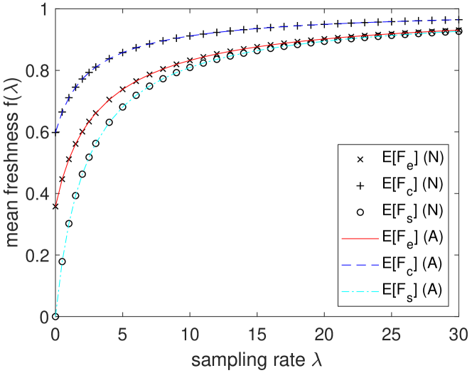
Figure 3: The mean freshness as a function of the sampling rate $\lambda$ for the FWE, FWC, and FWS freshness models using the numerical (N) and analytical (A) methods.

We compare our proposed water-willing solution, namely WF, with three baseline policies: i) UNIFORM policy samples each source-$n$ uniformly likely, i.e., $\lambda_{n}=\frac{\Lambda}{N}$, ii) PROP policy chooses the sampling rate $\lambda_{n}$ proportional with the source’s transition intensity $r_{n}$, i.e., $\lambda_{n}\propto r_{n}$, iii) INVPROP policy chooses the sampling rate $\lambda_{n}$ inversely proportional with the source’s transition intensity $r_{n}$, i.e., $\lambda_{n}\propto\frac{1}{r_{n}}$. Fig. 4 depicts the system freshness $F_{S}$ as a function of the sampling ratio $\kappa$ when the WF, UNIF, PROP, and INVPROP sampling policies are employed for both FWE and FWS freshness models. For both models, we observe that the WF policy outperforms all the other three baseline policies. The UNIFORM policy yields very close to optimum freshness performance when the sampling ratio increases. However, for low sampling ratios, it is substantially outperformed by the WF policy. The PROP and INVPROP sampling policies perform poorly for small and large sampling ratios, respectively, against all other policies.

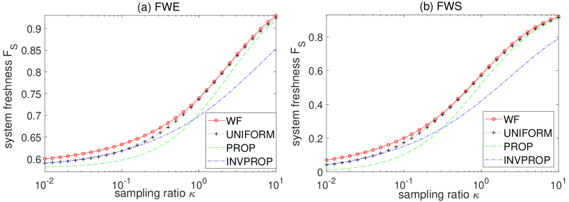
Figure 4: The system freshness $F_{S}$ as a function of the sampling ratio $\kappa$ for the WF, UNIFORM, PROP, and INVPROP sampling policies: (a) FWE (b) FWS.

Fig. 5 depicts the optimum sampling rate $\lambda_{n}$ divided by the sampling ratio $\kappa$ as a function of the source index $n$ for different values of the sampling ratio $\kappa$ for both freshness models. We observe that, for low sampling ratios, the water-filling solution chooses not to sample at all, a portion of the sources with high transition intensities, for both models. However, when the sampling ratio is sufficiently high, e.g., $\kappa=10$, the optimum sampling rate for a given source appears to be monotonically increasing with the transition intensity of the source. Although the general behavior of the optimum sampling rate with respect to source index is quite similar for FWE and FWS models, in the latter model, the optimum sampling rate is more uniform across the sources for FWS than FWE.

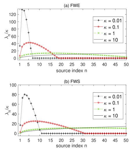
Figure 5: The optimum sampling rate $\lambda_{n}$ divided by $\kappa$ as a function of the source index $n$ for four values of the sampling ratio $\kappa$: (a) FWE (b) FWS.

In the final example, we focus on the FWC model and the choice of the proximity matrix $P$ in terms of a proximity parameter $v$ such that $p_{ij}=1$ when $|i-j|\leq v$, and is zero otherwise. It is clear that FWC with $v=0$ reduces to FWE. We consider an independent collection of $N$ CTMCs each of which corresponds to the number of active servers in a multi-server M/M/c/c queuing system with $c$ servers, with common service rate $\gamma$, and arrival rate $\xi_{n}$ for source-$n$. The load for source-$n$ is denoted by $\rho_{n}=\xi_{n}/c\gamma$. In this example, we assume linearly spaced loads, $\rho_{n}=\rho_{n-1}+\delta$, $n=2,\ldots,N$ and the parameter $\delta$ is chosen so that the average load is fixed to $\rho_{avg}=\frac{1}{N}\sum_{n=1}^{N}\rho_{n}$. In this example, we fix $\gamma=1$ and $\rho_{avg}=0.9$. The source weights are identical as in the previous examples. The overall sampling rate bound is taken as $\Lambda=20$. The weighted sum freshness $F_{S}=\frac{1}{N}\sum_{n=1}^{N}\mathbb{E}[F_{n,c}(t)]$ is plotted in Fig. 6 as a function of the number of users $N$ for FWC with the proximity parameter $v\in\{0,1,2,3\}$ and for two values of $\rho_{1}$ for the WF and UNIFORM policies. We have the following observations: When $\rho_{1}$ is close to $\rho_{avg}$, then all the sources have similar statistical behaviors and therefore the performances of WF and UNIFORM policies should be similar which is evident from Fig. 6(b). However, WF substantially outperforms the UNIFORM sampling policy in Fig. 6(a) where the smallest load source-1 has a load $\rho_{1}=0.01$ and consequently the sources are statistically dissimilar from each other. We have observed similar outperformance behavior of WF over the UNIFORM policy for the four values of the proximity parameter $v$ we have investigated. The weighted sum freshness decreases with increased $N$ since the sampling rate parameter $\Lambda$ is fixed for any choice of $N$. Therefore, sources are sampled at a lower intensity, on the average, as $N$ is increased in our example.

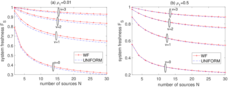
Figure 6: System freshness $F_{S}$ for the FWC model as a function of the number of users, $N$, for the WF and UNIFORM sampling policies for four different choices of the proximity matrix, i.e., $v\in\{0,1,2,3\}$.

VII Conclusions

We investigated a remote monitoring system which samples a set of ergodic and aperiodic CTMCs according to a Poisson process, under an overall sampling rate constraint, employing a remote martingale estimate of the states of each of the CTMCs. Three binary freshness models are studied and expressions for mean freshness are obtained for all the freshness models of interest. Subsequently, the optimum sampling rates for all CTMCs are obtained using water-filling based optimization while maximizing the weighted sum freshness. The worst case computational complexity of the proposed method is quadratic in the number of CTMCs making it possible to solve for scenarios even with very large numbers of CTMCs. The optimum monitoring policy is shown to outperform a number of heuristic baseline policies especially when there is diversity in the statistical characteristics of the underlying sources.

Future work will consist of the study of estimators other than the martingale estimator, Markov information sources other than CTMCs, and the case of information sources whose statistical characterization is partially known, or is not known at all. It is also interesting to study how the gains attained in weighted sum freshness by the proposed method are to be reflected in the actual performance of the underlying application. Another potential research direction is to take into consideration the most recently taken sample values while making a decision of which source to sample.

References

- [1] S. Kaul, R. Yates, and M. Gruteser, “Real-time status: How often should one update?” in IEEE Infocom, March 2012.
- [2] A. Kosta, N. Pappas, and V. Angelakis, “Age of information: A new concept, metric, and tool,” Foundations and Trends in Networking, vol. 12, no. 3, pp. 162–259, 2017.
- [3] R. D. Yates, Y. Sun, D. R. Brown, S. K. Kaul, E. Modiano, and S. Ulukus, “Age of information: An introduction and survey,” IEEE Journal on Selected Areas in Communications, vol. 39, no. 5, pp. 1183–1210, May 2021.
- [4] M. Costa, M. Codreanu, and A. Ephremides, “Age of information with packet management,” in IEEE ISIT, June 2014.
- [5] N. Akar and E. Karasan, “Is proportional fair scheduling suitable for age-sensitive traffic?” Computer Networks, vol. 226, p. 109668, 2023.
- [6] A. Kosta, N. Pappas, A. Ephremides, and V. Angelakis, “Non-linear age of information in a discrete time queue: Stationary distribution and average performance analysis,” in IEEE ICC, June 2020.
- [7] N. Akar and O. Dogan, “Discrete-time queueing model of age of information with multiple information sources,” IEEE Internet of Things Journal, vol. 8, no. 19, pp. 14 531–14 542, October 2021.
- [8] R. D. Yates and S. K. Kaul, “The age of information: Real-time status updating by multiple sources,” IEEE Transactions on Information Theory, vol. 65, no. 3, pp. 1807–1827, March 2019.
- [9] M. Moltafet, M. Leinonen, and M. Codreanu, “On the age of information in multi-source queueing models,” IEEE Transactions on Communications, vol. 68, no. 8, pp. 5003–5017, August 2020.
- [10] E. O. Gamgam and N. Akar, “Exact analytical model of age of information in multi-source status update systems with per-source queueing,” IEEE Internet of Things Journal, vol. 9, no. 20, pp. 20 706–20 718, October 2022.
- [11] Y. Sang, B. Li, and B. Ji, “The power of waiting for more than one response in minimizing the age-of-information,” in IEEE Globecom, December 2017.
- [12] F. Li, Y. Sang, Z. Liu, B. Li, H. Wu, and B. Ji, “Waiting but not aging: Optimizing information freshness under the pull model,” IEEE/ACM Transactions on Networking, vol. 29, no. 1, pp. 465–478, February 2021.
- [13] J. Cho and H. Garcia-Molina, “Effective page refresh policies for web crawlers,” ACM Transactions on Database Systems, vol. 28, no. 4, p. 390–426, December 2003.
- [14] M. Bastopcu and S. Ulukus, “Maximizing information freshness in caching systems with limited cache storage capacity,” in Asilomar Conference on Signals, Systems, and Computers, November 2020.
- [15] P. Kaswan, M. Bastopcu, and S. Ulukus, “Freshness based cache updating in parallel relay networks,” in IEEE ISIT, July 2021.
- [16] M. Bastopcu and S. Ulukus, “Information freshness in cache updating systems,” IEEE Transactions on Wireless Communications, vol. 20, no. 3, pp. 1861–1874, March 2021.
- [17] M. Bastopcu, B. Buyukates, and S. Ulukus, “Gossiping with binary freshness metric,” in IEEE Globecom, December 2021.
- [18] B. Abolhassani, J. Tadrous, A. Eryilmaz, and E. Yeh, “Fresh caching for dynamic content,” in IEEE Infocom, May 2021.
- [19] R. D. Yates, “The age of gossip in networks,” in IEEE ISIT, July 2021.
- [20] M. Bastopcu and S. Ulukus, “Who should Google Scholar update more often?” in IEEE Infocom, July 2020.
- [21] B. Buyukates, M. Bastopcu, and S. Ulukus, “Age of gossip in networks with community structure,” in IEEE SPAWC, September 2021.
- [22] J. Zhong, R. D. Yates, and E. Soljanin, “Two freshness metrics for local cache refresh,” in IEEE ISIT, June 2018.
- [23] H. Tang, J. Wang, Z. Tang, and J. Song, “Scheduling to minimize age of synchronization in wireless broadcast networks with random updates,” in IEEE ISIT, July 2019.
- [24] C. Deng, J. Yang, and C. Pan, “Timely synchronization with sporadic status changes,” in IEEE ICC, June 2020.
- [25] R. G. Gallager, Stochastic Processes: Theory for Applications. Cambridge University Press, 2013.
- [26] D. Palomar and J. Fonollosa, “Practical algorithms for a family of waterfilling solutions,” IEEE Transactions on Signal Processing, vol. 53, no. 2, pp. 686–695, February 2005.
- [27] C. Xing, Y. Jing, S. Wang, S. Ma, and H. V. Poor, “New viewpoint and algorithms for water-filling solutions in wireless communications,” IEEE Transactions on Signal Processing, vol. 68, pp. 1618–1634, February 2020.
- [28] D. Palomar and M. Lagunas, “Joint transmit-receive space-time equalization in spatially correlated MIMO channels: a beamforming approach,” IEEE Journal on Selected Areas in Communications, vol. 21, no. 5, pp. 730–743, June 2003.
- [29] O. Ozel, K. Tutuncuoglu, J. Yang, S. Ulukus, and A. Yener, “Transmission with energy harvesting nodes in fading wireless channels: Optimal policies,” IEEE Journal on Selected Areas in Communications, vol. 29, no. 8, pp. 1732–1743, September 2011.
- [30] K. Huang, W. Liu, M. Shirvanimoghaddam, Y. Li, and B. Vucetic, “Real-time remote estimation with hybrid ARQ in wireless networked control,” IEEE Transactions on Wireless Communications, vol. 19, no. 5, pp. 3490–3504, May 2020.
- [31] Y. Sun, Y. Polyanskiy, and E. Uysal, “Sampling of the Wiener process for remote estimation over a channel with random delay,” IEEE Transactions on Information Theory, vol. 66, no. 2, pp. 1118–1135, February 2020.
- [32] N. Pappas and M. Kountouris, “Goal-oriented communication for real-time tracking in autonomous systems,” in IEEE ICAS, August 2021.
- [33] E. Fountoulakis, N. Pappas, and M. Kountouris, “Goal-oriented policies for cost of actuation error minimization in wireless autonomous systems,” IEEE Communications Letters, vol. 27, no. 9, pp. 2323–2327, September 2023.
- [34] J. P. Champati, M. Skoglund, M. Jansson, and J. Gross, “Detecting state transitions of a Markov source: Sampling frequency and age trade-off,” IEEE Transactions on Communications, vol. 70, no. 5, pp. 3081–3095, May 2022.
- [35] Y. Inoue and T. Takine, “AoI perspective on the accuracy of monitoring systems for continuous-time Markovian sources,” in IEEE Infocom, April 2019.
- [36] M. Bastopcu and S. Ulukus, “Using timeliness in tracking infections,” Entropy, vol. 24, no. 6, p. 779, May 2022.
- [37] M. Harchol-Balter, Performance Modeling and Design of Computer Systems: Queueing Theory in Action, 1st ed. Cambridge University Press, 2013.