\newcites
suppSupplemental References
† † thanks: These two authors contributed equally† † thanks: These two authors contributed equally
Symmetry-based classification of exact flat bands in single and bilayer moiré systems
Siddhartha Sarkar
Department of Physics, University of Michigan, Ann Arbor, MI 48109, USA
Xiaohan Wan
Department of Physics, University of Michigan, Ann Arbor, MI 48109, USA
Shi-Zeng Lin
szl@lanl.gov
Theoretical Division, T-4 and CNLS, Los Alamos National Laboratory, Los Alamos, New Mexico 87545, USA
Center for Integrated Nanotechnologies (CINT), Los Alamos National Laboratory, Los Alamos, New Mexico 87545, USA
Kai Sun
sunkai@umich.edu
Department of Physics, University of Michigan, Ann Arbor, MI 48109, USA
Abstract
We study the influence of spatial symmetries on the appearance and the number of exact flat bands (FBs) in single and bilayer systems with Dirac or quadratic band crossing points, and
systematically classify all possible number of exact flat bands in systems with different point group symmetries.
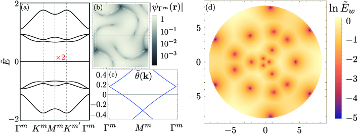
We find that a maximum of 6 FBs can be protected by symmetries, and show an example of 6 FBs in a system with QBCP under periodic strain field of 𝒞 6 v subscript 𝒞 6 𝑣 \mathcal{C}_{6v} ℤ 2 subscript ℤ 2 \mathds{Z}_{2} C = 1 𝐶 1 C=1 C = − 1 𝐶 1 C=-1
Introduction. –The interplay between topology and strong interaction makes topological flat bands(FBs) ideal for nontrivial states such as fractional Chern insulators, high T c subscript 𝑇 𝑐 T_{c} Tarnopolsky et al. (2019 ) showed that, in the chiral limit of TBG, where the AA tunneling is set to zero, the middle two bands at the Fermi level become exactly flat at certain magic angles. They also showed that the exact wave-functions(WFs) of these two bands are complex analytic functions, analogous to WFs of the lowest Landau level (LLL) on a torus Haldane and Rezayi (1985 ) . Just like LLL WFs, the analytic WFs of chiral TBG also carry Chern number C = ± 1 𝐶 plus-or-minus 1 C=\pm 1 Li et al. (2022 ) , TBG with spatially alternating magnetic field Becker et al. (2022 ); Le et al. (2022 ) , single layer system with quadratic band crossing point (QBCP) under periodic strain field Wan et al. (2023 ) , twisted bilayer Fe-based superlattices Eugenio and Vafek (2023 ) , and TBG with strong second harmonic tunneling Becker et al. (2023 ) . Curiously, even though the origin of the exact FBs in all these systems are same, there are some tangible differences between the exact FBs reported in these articles. Firstly, in some cases the number of FBs are doubled Becker et al. (2022 ); Le et al. (2022 ); Wan et al. (2023 ); Becker et al. (2023 ) . Second, in case of TBCL, the Chern number is C = ± 2 𝐶 plus-or-minus 2 C=\pm 2 ± 1 plus-or-minus 1 \pm 1 Neupert et al. (2011 ); Qi (2011 ); Wang and Ran (2011 ); Wang et al. (2012 ); Yang et al. (2012 ); Wu et al. (2013 ); Andrews and Soluyanov (2020 ); Liu et al. (2021 ); Andrews et al. (2021 ); Zhang et al. (2019 ) .
However, the different number of FBs and different Chern numbers lead to puzzles. To get a better understanding, let us describe the origin of the exact FBs in these systems. The general form of the 𝐤 ⋅ 𝐩 ⋅ 𝐤 𝐩 \mathbf{k}\cdot\mathbf{p}
ℋ ( 𝐫 ) = ( 𝟎 𝒟 † ( 𝐫 ) 𝒟 ( 𝐫 ) 𝟎 ) ℋ 𝐫 matrix 0 superscript 𝒟 † 𝐫 𝒟 𝐫 0 \mathcal{H}(\mathbf{r})=\begin{pmatrix}\mathbf{0}&\mathcal{D}^{\dagger}(\mathbf{r})\\
\mathcal{D}(\mathbf{r})&\mathbf{0}\end{pmatrix} (1)
near a high symmetry momentum (HSM) 𝐤 0 subscript 𝐤 0 \mathbf{k}_{0} 𝐤 0 subscript 𝐤 0 \mathbf{k}_{0} n 𝑛 n 𝒞 n z subscript 𝒞 𝑛 𝑧 \mathcal{C}_{nz} n = 3 𝑛 3 n=3 n = 3 𝑛 3 n=3 4 4 4 𝒜 𝒜 \mathcal{A} = 𝒯 absent 𝒯 =\mathcal{T} = 𝒞 2 z 𝒯 absent subscript 𝒞 2 𝑧 𝒯 =\mathcal{C}_{2z}\mathcal{T} 𝒯 𝒯 \mathcal{T} 𝒜 𝐫 = ± 𝐫 𝒜 𝐫 plus-or-minus 𝐫 \mathcal{A}\mathbf{r}=\pm\mathbf{r} 𝒜 𝐤 = ∓ 𝐤 𝒜 𝐤 minus-or-plus 𝐤 \mathcal{A}\mathbf{k}=\mp\mathbf{k} 𝒜 = 𝒯 𝒜 𝒯 \mathcal{A}=\mathcal{T} 𝒞 2 z 𝒯 subscript 𝒞 2 𝑧 𝒯 \mathcal{C}_{2z}\mathcal{T} 𝒜 𝐤 0 ≡ 𝐤 0 𝒜 subscript 𝐤 0 subscript 𝐤 0 \mathcal{A}\mathbf{k}_{0}\equiv\mathbf{k}_{0} 𝒟 ( 𝐫 ) 𝒟 𝐫 \mathcal{D}(\mathbf{r}) l × l 𝑙 𝑙 l\times l l 𝑙 l 𝒟 ( 𝐫 ) 𝒟 𝐫 \mathcal{D}(\mathbf{r}) 𝒟 k ( 𝐫 ) subscript 𝒟 𝑘 𝐫 \mathcal{D}_{k}(\mathbf{r}) D U ( 𝐫 ; 𝜶 ) subscript 𝐷 𝑈 𝐫 𝜶
D_{U}(\mathbf{r};\bm{\alpha}) Tarnopolsky et al. (2019 ); Li et al. (2022 ); Becker et al. (2022 ); Le et al. (2022 ); Eugenio and Vafek (2023 ); Becker et al. (2023 ) or externally applied field Le et al. (2022 ); Wan et al. (2023 ) , and 𝜶 𝜶 \bm{\alpha} 𝒟 k ( 𝐫 ) = ( − 2 i ∂ z ¯ ) m 𝟙 subscript 𝒟 𝑘 𝐫 superscript 2 𝑖 ¯ subscript 𝑧 𝑚 1 \mathcal{D}_{k}(\mathbf{r})=(-2i\overline{\partial_{z}})^{m}\mathds{1} z = x + i y 𝑧 𝑥 𝑖 𝑦 z=x+iy 𝟙 1 \mathds{1} ∗ stands for complex conjugation, and m = 1 𝑚 1 m=1 2 2 2 𝒞 n z subscript 𝒞 𝑛 𝑧 \mathcal{C}_{nz} 𝒟 ( 𝐫 ) = 𝒟 k ( 𝐫 ) + 𝒟 U ( 𝐫 ; 𝜶 ) 𝒟 𝐫 subscript 𝒟 𝑘 𝐫 subscript 𝒟 𝑈 𝐫 𝜶
\mathcal{D}(\mathbf{r})=\mathcal{D}_{k}(\mathbf{r})+\mathcal{D}_{U}(\mathbf{r};\bm{\alpha}) 𝒟 ( 𝒞 n z 𝐫 ) = ( ω ∗ ) 2 𝒟 ( 𝐫 ) 𝒟 subscript 𝒞 𝑛 𝑧 𝐫 superscript superscript 𝜔 2 𝒟 𝐫 \mathcal{D}(\mathcal{C}_{nz}\mathbf{r})=(\omega^{*})^{2}\mathcal{D}(\mathbf{r}) ω = e 2 π i ( m + 3 ) / n 𝜔 superscript 𝑒 2 𝜋 𝑖 𝑚 3 𝑛 \omega=e^{2\pi i(m+3)/n} Diag { ω 𝟙 , ω ∗ 𝟙 } ℋ ( 𝐫 ) Diag { ω ∗ 𝟙 , ω 𝟙 } = ℋ ( 𝒞 n z 𝐫 ) Diag 𝜔 1 superscript 𝜔 1 ℋ 𝐫 Diag superscript 𝜔 1 𝜔 1 ℋ subscript 𝒞 𝑛 𝑧 𝐫 \text{Diag}\{\omega\mathds{1},\omega^{*}\mathds{1}\}\mathcal{H}(\mathbf{r})\text{Diag}\{\omega^{*}\mathds{1},\omega\mathds{1}\}=\mathcal{H}(\mathcal{C}_{nz}\mathbf{r}) 𝒜 𝒜 \mathcal{A} σ x ⊗ 𝟙 ℋ ∗ ( 𝐫 ) σ x ⊗ 𝟙 = ℋ ( 𝒜 𝐫 ) tensor-product tensor-product subscript 𝜎 𝑥 1 superscript ℋ 𝐫 subscript 𝜎 𝑥 1 ℋ 𝒜 𝐫 \sigma_{x}\otimes\mathds{1}\mathcal{H}^{*}(\mathbf{r})\sigma_{x}\otimes\mathds{1}=\mathcal{H}(\mathcal{A}\mathbf{r}) see Supplemental Material (SM) SM (2 ) Sec. S-I for more details ). An exact FB of ℋ ( 𝐫 ) ℋ 𝐫 \mathcal{H}(\mathbf{r}) E = 0 𝐸 0 E=0 Ψ 𝐤 ( 𝐫 ) subscript Ψ 𝐤 𝐫 \Psi_{\mathbf{k}}(\mathbf{r}) ℋ ( 𝐫 ) Ψ 𝐤 ( 𝐫 ) = 𝟎 ℋ 𝐫 subscript Ψ 𝐤 𝐫 0 \mathcal{H}(\mathbf{r})\Psi_{\mathbf{k}}(\mathbf{r})=\mathbf{0} 𝐤 𝐤 \mathbf{k} Ψ 𝐤 ( 𝐫 ) subscript Ψ 𝐤 𝐫 \Psi_{\mathbf{k}}(\mathbf{r}) 𝒞 n z subscript 𝒞 𝑛 𝑧 \mathcal{C}_{nz} 𝒮 = σ z ⊗ 𝟙 𝒮 tensor-product subscript 𝜎 𝑧 1 \mathcal{S}=\sigma_{z}\otimes\mathds{1} 𝐤 0 m superscript subscript 𝐤 0 𝑚 \mathbf{k}_{0}^{m} 𝐤 0 subscript 𝐤 0 \mathbf{k}_{0} 𝐤 0 m superscript subscript 𝐤 0 𝑚 \mathbf{k}_{0}^{m} E = 0 𝐸 0 E=0 𝒟 U ( 𝐫 ; 𝜶 ) subscript 𝒟 𝑈 𝐫 𝜶
\mathcal{D}_{U}(\mathbf{r};\bm{\alpha}) 𝒞 n z subscript 𝒞 𝑛 𝑧 \mathcal{C}_{nz} Ψ 𝐤 0 m , 1 ( 𝐫 ) = { ψ 𝐤 0 m ( 𝐫 ) , 𝟎 } subscript Ψ superscript subscript 𝐤 0 𝑚 1
𝐫 subscript 𝜓 superscript subscript 𝐤 0 𝑚 𝐫 0 \Psi_{\mathbf{k}_{0}^{m},1}(\mathbf{r})=\{\psi_{\mathbf{k}_{0}^{m}}(\mathbf{r}),\mathbf{0}\} Ψ 𝐤 0 m , 2 ( 𝐫 ) = { 𝟎 , ψ 𝐤 0 m ∗ ( 𝒜 𝐫 ) } subscript Ψ superscript subscript 𝐤 0 𝑚 2
𝐫 0 superscript subscript 𝜓 superscript subscript 𝐤 0 𝑚 𝒜 𝐫 \Psi_{\mathbf{k}_{0}^{m},2}(\mathbf{r})=\{\mathbf{0},\psi_{\mathbf{k}_{0}^{m}}^{*}(\mathcal{A}\mathbf{r})\} ℋ ( 𝐫 ) Ψ 𝐤 0 m , i ( 𝐫 ) = 𝟎 ℋ 𝐫 subscript Ψ superscript subscript 𝐤 0 𝑚 𝑖
𝐫 0 \mathcal{H}(\mathbf{r})\Psi_{\mathbf{k}_{0}^{m},i}(\mathbf{r})=\mathbf{0} 𝒟 ( 𝐫 ) ψ 𝐤 0 m ( 𝐫 ) = 𝟎 𝒟 𝐫 subscript 𝜓 superscript subscript 𝐤 0 𝑚 𝐫 0 \mathcal{D}(\mathbf{r})\psi_{\mathbf{k}_{0}^{m}}(\mathbf{r})=\mathbf{0} { ψ 𝐤 ( 𝐫 ) , 𝟎 } subscript 𝜓 𝐤 𝐫 0 \{\psi_{\mathbf{k}}(\mathbf{r}),\mathbf{0}\} { 𝟎 , ψ 𝒜 𝐤 ∗ ( 𝒜 𝐫 ) } 0 superscript subscript 𝜓 𝒜 𝐤 𝒜 𝐫 \{\mathbf{0},\psi_{\mathcal{A}\mathbf{k}}^{*}(\mathcal{A}\mathbf{r})\} 𝒟 k ( 𝐫 ) subscript 𝒟 𝑘 𝐫 \mathcal{D}_{k}(\mathbf{r}) ψ 𝐤 + 𝐤 0 m ( 𝐫 ) = f 𝐤 ( z ) ψ 𝐤 0 m ( 𝐫 ) subscript 𝜓 𝐤 superscript subscript 𝐤 0 𝑚 𝐫 subscript 𝑓 𝐤 𝑧 subscript 𝜓 superscript subscript 𝐤 0 𝑚 𝐫 \psi_{\mathbf{k}+\mathbf{k}_{0}^{m}}(\mathbf{r})=f_{\mathbf{k}}(z)\psi_{\mathbf{k}_{0}^{m}}(\mathbf{r}) f 𝐤 ( z ) subscript 𝑓 𝐤 𝑧 f_{\mathbf{k}}(z) ∂ z ¯ f 𝐤 ( z ) = 0 ¯ subscript 𝑧 subscript 𝑓 𝐤 𝑧 0 \overline{\partial_{z}}f_{\mathbf{k}}(z)=0 f 𝐤 ( z ) subscript 𝑓 𝐤 𝑧 f_{\mathbf{k}}(z) 𝐚 m superscript 𝐚 𝑚 \mathbf{a}^{m} e i 𝐤 ⋅ 𝐚 m superscript 𝑒 ⋅ 𝑖 𝐤 superscript 𝐚 𝑚 e^{i\mathbf{k}\cdot\mathbf{a}^{m}} ψ 𝐤 ( 𝐫 ) subscript 𝜓 𝐤 𝐫 \psi_{\mathbf{k}}(\mathbf{r}) ψ 𝐤 0 m ( 𝐫 ) subscript 𝜓 superscript subscript 𝐤 0 𝑚 𝐫 \psi_{\mathbf{k}_{0}^{m}}(\mathbf{r}) ψ 𝐤 0 m ( 𝐫 ) subscript 𝜓 superscript subscript 𝐤 0 𝑚 𝐫 \psi_{\mathbf{k}_{0}^{m}}(\mathbf{r}) 𝐫 0 subscript 𝐫 0 \mathbf{r}_{0}
f 𝐤 ( z ; 𝐫 0 ) = e i ( 𝐤 ⋅ 𝐚 1 m ) z / a 1 ϑ ( z − z 0 a 1 m − k b 2 m , τ ) ϑ ( z − z 0 a 1 m , τ ) = e i 𝐤 ⋅ 𝐫 f ~ 𝐤 ( 𝐫 ; 𝐫 0 ) , f ~ 𝐤 ( 𝐫 ; 𝐫 0 ) = e − i ( 𝐛 2 m ⋅ 𝐫 ) k / b 2 m ϑ ( z − z 0 a 1 m − k b 2 m , τ ) ϑ ( z − z 0 a 1 m , τ ) formulae-sequence subscript 𝑓 𝐤 𝑧 subscript 𝐫 0
superscript 𝑒 𝑖 ⋅ 𝐤 subscript superscript 𝐚 𝑚 1 𝑧 subscript 𝑎 1 italic-ϑ 𝑧 subscript 𝑧 0 superscript subscript 𝑎 1 𝑚 𝑘 superscript subscript 𝑏 2 𝑚 𝜏 italic-ϑ 𝑧 subscript 𝑧 0 superscript subscript 𝑎 1 𝑚 𝜏 superscript 𝑒 ⋅ 𝑖 𝐤 𝐫 subscript ~ 𝑓 𝐤 𝐫 subscript 𝐫 0
subscript ~ 𝑓 𝐤 𝐫 subscript 𝐫 0
superscript 𝑒 𝑖 ⋅ superscript subscript 𝐛 2 𝑚 𝐫 𝑘 superscript subscript 𝑏 2 𝑚 italic-ϑ 𝑧 subscript 𝑧 0 superscript subscript 𝑎 1 𝑚 𝑘 superscript subscript 𝑏 2 𝑚 𝜏 italic-ϑ 𝑧 subscript 𝑧 0 superscript subscript 𝑎 1 𝑚 𝜏 \begin{split}&f_{\mathbf{k}}(z;\mathbf{r}_{0})=e^{i(\mathbf{k}\cdot\mathbf{a}^{m}_{1})z/a_{1}}\frac{\vartheta\left(\frac{z-z_{0}}{a_{1}^{m}}-\frac{k}{b_{2}^{m}},\tau\right)}{\vartheta\left(\frac{z-z_{0}}{a_{1}^{m}},\tau\right)}\\
&\hskip 36.98866pt=e^{i\mathbf{k}\cdot\mathbf{r}}\tilde{f}_{\mathbf{k}}(\mathbf{r};\mathbf{r}_{0}),\\
&\tilde{f}_{\mathbf{k}}(\mathbf{r};\mathbf{r}_{0})=e^{-i(\mathbf{b}_{2}^{m}\cdot\mathbf{r})k/b_{2}^{m}}\frac{\vartheta\left(\frac{z-z_{0}}{a_{1}^{m}}-\frac{k}{b_{2}^{m}},\tau\right)}{\vartheta\left(\frac{z-z_{0}}{a_{1}^{m}},\tau\right)}\end{split} (2)
with a pole at 𝐫 0 subscript 𝐫 0 \mathbf{r}_{0} ϑ ( z , τ ) italic-ϑ 𝑧 𝜏 \vartheta(z,\tau) Ledwith et al. (2020 ) , 𝐚 i m subscript superscript 𝐚 𝑚 𝑖 \mathbf{a}^{m}_{i} 𝐛 i m subscript superscript 𝐛 𝑚 𝑖 \mathbf{b}^{m}_{i} 𝐚 i m ⋅ 𝐛 j m = 2 π δ i j ⋅ subscript superscript 𝐚 𝑚 𝑖 subscript superscript 𝐛 𝑚 𝑗 2 𝜋 subscript 𝛿 𝑖 𝑗 \mathbf{a}^{m}_{i}\cdot\mathbf{b}^{m}_{j}=2\pi\delta_{ij} a i m = ( 𝐚 i m ) x + i ( 𝐚 i m ) y superscript subscript 𝑎 𝑖 𝑚 subscript subscript superscript 𝐚 𝑚 𝑖 𝑥 𝑖 subscript subscript superscript 𝐚 𝑚 𝑖 𝑦 a_{i}^{m}=(\mathbf{a}^{m}_{i})_{x}+i(\mathbf{a}^{m}_{i})_{y} b i m = ( 𝐛 i m ) x + i ( 𝐛 i m ) y superscript subscript 𝑏 𝑖 𝑚 subscript subscript superscript 𝐛 𝑚 𝑖 𝑥 𝑖 subscript subscript superscript 𝐛 𝑚 𝑖 𝑦 b_{i}^{m}=(\mathbf{b}^{m}_{i})_{x}+i(\mathbf{b}^{m}_{i})_{y} z 0 = ( 𝐫 0 ) x + i ( 𝐫 0 ) y subscript 𝑧 0 subscript subscript 𝐫 0 𝑥 𝑖 subscript subscript 𝐫 0 𝑦 z_{0}=(\mathbf{r}_{0})_{x}+i(\mathbf{r}_{0})_{y} k = k x + i k y 𝑘 subscript 𝑘 𝑥 𝑖 subscript 𝑘 𝑦 k=k_{x}+ik_{y} τ = a 2 m / a 1 m 𝜏 superscript subscript 𝑎 2 𝑚 superscript subscript 𝑎 1 𝑚 \tau=a_{2}^{m}/a_{1}^{m} 𝜶 𝜶 \bm{\alpha} ψ 𝐤 0 m ( 𝐫 ) subscript 𝜓 superscript subscript 𝐤 0 𝑚 𝐫 \psi_{\mathbf{k}_{0}^{m}}(\mathbf{r}) f 𝐤 ( z ; 𝐫 0 ) subscript 𝑓 𝐤 𝑧 subscript 𝐫 0
f_{\mathbf{k}}(z;\mathbf{r}_{0}) f ~ 𝐤 ( 𝐫 ; 𝐫 0 ) subscript ~ 𝑓 𝐤 𝐫 subscript 𝐫 0
\tilde{f}_{\mathbf{k}}(\mathbf{r};\mathbf{r}_{0}) k 𝑘 k Kharchev and Zabrodin (2015 ); Ledwith et al. (2020 ) ; this property along with the presence of the zero in the WF can be used to prove that wave functions of this form carry Chern number C = ± 1 𝐶 plus-or-minus 1 C=\pm 1 Wang et al. (2021a ) , also SM SM (2 ) S-IV for a proof ).
It was found in Wan et al. (2023 ) , that in some cases ψ 𝐤 0 m ( 𝐫 ) subscript 𝜓 superscript subscript 𝐤 0 𝑚 𝐫 \psi_{\mathbf{k}_{0}^{m}}(\mathbf{r}) 𝐫 0 ( 1 ) superscript subscript 𝐫 0 1 \mathbf{r}_{0}^{(1)} 𝐫 0 ( 2 ) superscript subscript 𝐫 0 2 \mathbf{r}_{0}^{(2)} f 𝐤 ( z ; 𝐫 0 ( 1 ) ) subscript 𝑓 𝐤 𝑧 superscript subscript 𝐫 0 1
f_{\mathbf{k}}(z;\mathbf{r}_{0}^{(1)}) f 𝐤 ( z ; 𝐫 0 ( 2 ) ) subscript 𝑓 𝐤 𝑧 superscript subscript 𝐫 0 2
f_{\mathbf{k}}(z;\mathbf{r}_{0}^{(2)}) 𝐫 0 ( 1 ) superscript subscript 𝐫 0 1 \mathbf{r}_{0}^{(1)} 𝐫 0 ( 2 ) superscript subscript 𝐫 0 2 \mathbf{r}_{0}^{(2)} ψ 𝐤 0 m ( 𝐫 ) subscript 𝜓 superscript subscript 𝐤 0 𝑚 𝐫 \psi_{\mathbf{k}_{0}^{m}}(\mathbf{r}) ψ 𝐤 0 m ( 𝐫 ) subscript 𝜓 superscript subscript 𝐤 0 𝑚 𝐫 \psi_{\mathbf{k}_{0}^{m}}(\mathbf{r}) Le et al. (2022 ) ; four FBs were found even though ψ 𝐤 0 m ( 𝐫 ) subscript 𝜓 superscript subscript 𝐤 0 𝑚 𝐫 \psi_{\mathbf{k}_{0}^{m}}(\mathbf{r})
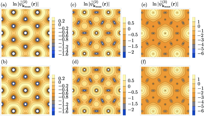
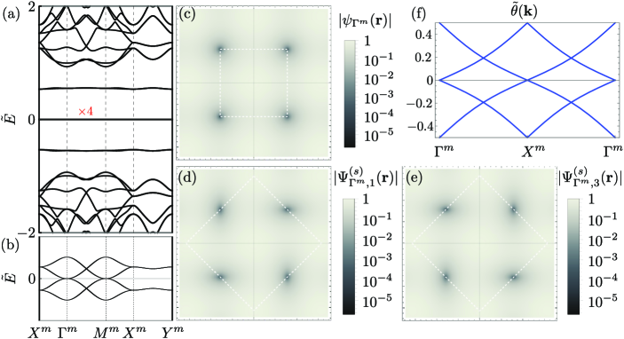
Figure 1: Different number of exact flat bands in single layer system with QBCP under different periodic strain fields A ~ ( 𝐫 ) ~ 𝐴 𝐫 \tilde{A}(\mathbf{r}) p 6 m m 𝑝 6 𝑚 𝑚 p6mm A ~ ( 𝐫 ) = − α 2 ∑ n = 1 3 e i ( 4 − n ) ϕ cos ( 𝐛 n m ⋅ 𝐫 ) ~ 𝐴 𝐫 𝛼 2 superscript subscript 𝑛 1 3 superscript 𝑒 𝑖 4 𝑛 italic-ϕ ⋅ superscript subscript 𝐛 𝑛 𝑚 𝐫 \tilde{A}(\mathbf{r})=-\frac{\alpha}{2}\sum_{n=1}^{3}e^{i(4-n)\phi}\cos\left(\mathbf{b}_{n}^{m}\cdot\mathbf{r}\right) A ~ ( 𝐫 ) = − α 2 ∑ n = 1 3 ( − e i ( 1 − n ) ϕ cos ( 2 𝐛 n m ⋅ 𝐫 ) + 2 e i ( 2 − n ) ϕ cos ( ( 𝐛 n m − 𝐛 n + 1 m ) ⋅ 𝐫 ) + 2 e i ( 4 − n ) ϕ cos ( 𝐛 n m ⋅ 𝐫 ) ) ~ 𝐴 𝐫 𝛼 2 superscript subscript 𝑛 1 3 superscript 𝑒 𝑖 1 𝑛 italic-ϕ ⋅ 2 superscript subscript 𝐛 𝑛 𝑚 𝐫 2 superscript 𝑒 𝑖 2 𝑛 italic-ϕ ⋅ superscript subscript 𝐛 𝑛 𝑚 superscript subscript 𝐛 𝑛 1 𝑚 𝐫 2 superscript 𝑒 𝑖 4 𝑛 italic-ϕ ⋅ superscript subscript 𝐛 𝑛 𝑚 𝐫 \tilde{A}(\mathbf{r})=-\frac{\alpha}{2}\sum_{n=1}^{3}(-e^{i(1-n)\phi}\cos\left(2\mathbf{b}_{n}^{m}\cdot\mathbf{r}\right)+2e^{i(2-n)\phi}\cos\left((\mathbf{b}_{n}^{m}-\mathbf{b}_{n+1}^{m})\cdot\mathbf{r}\right)+2e^{i(4-n)\phi}\cos\left(\mathbf{b}_{n}^{m}\cdot\mathbf{r}\right)) ϕ = 2 π / 3 italic-ϕ 2 𝜋 3 \phi=2\pi/3 𝐛 1 m = 4 π 3 a m ( 0 , 1 ) subscript superscript 𝐛 𝑚 1 4 𝜋 3 superscript 𝑎 𝑚 0 1 \mathbf{b}^{m}_{1}=\frac{4\pi}{\sqrt{3}a^{m}}(0,1) 𝐛 2 , 3 m = 4 π 3 a m ( ∓ 3 / 2 , − 1 / 2 ) subscript superscript 𝐛 𝑚 2 3
4 𝜋 3 superscript 𝑎 𝑚 minus-or-plus 3 2 1 2 \mathbf{b}^{m}_{2,3}=\frac{4\pi}{\sqrt{3}a^{m}}(\mp\sqrt{3}/2,-1/2) a m superscript 𝑎 𝑚 a^{m} E ~ = E | 𝐛 m | 2 ~ 𝐸 𝐸 superscript superscript 𝐛 𝑚 2 \tilde{E}=\frac{E}{|\mathbf{b}^{m}|^{2}} α 𝛼 \alpha α ~ = α | 𝐛 m | 2 = 0.62 , − 2.88 formulae-sequence ~ 𝛼 𝛼 superscript superscript 𝐛 𝑚 2 0.62 2.88 \tilde{\alpha}=\frac{\alpha}{|\mathbf{b}^{m}|^{2}}=0.62,-2.88 2.93 2.93 2.93 | ψ Γ m ( 𝐫 ) | subscript 𝜓 superscript Γ 𝑚 𝐫 |\psi_{\Gamma^{m}}(\mathbf{r})| θ ~ ( 𝐤 ) = θ ( 𝐤 ) 2 π ~ 𝜃 𝐤 𝜃 𝐤 2 𝜋 \tilde{\theta}({\mathbf{k}})=\frac{\theta({\mathbf{k}})}{2\pi}
In this article, we show that not all zeros of ψ 𝐤 0 m ( 𝐫 ) subscript 𝜓 superscript subscript 𝐤 0 𝑚 𝐫 \psi_{\mathbf{k}_{0}^{m}}(\mathbf{r}) 𝒞 n ′ z subscript 𝒞 superscript 𝑛 ′ 𝑧 \mathcal{C}_{n^{\prime}z} n ′ ≥ 2 superscript 𝑛 ′ 2 n^{\prime}\geq 2 3 𝒞 6 subscript 𝒞 6 \mathcal{C}_{6} 𝒞 6 v subscript 𝒞 6 𝑣 \mathcal{C}_{6v} 𝒞 6 v subscript 𝒞 6 𝑣 \mathcal{C}_{6v} C = ± 2 𝐶 plus-or-minus 2 C=\pm 2 Li et al. (2022 ) .
Only the zeros of ψ 𝐤 0 m ( 𝐫 ) subscript 𝜓 superscript subscript 𝐤 0 𝑚 𝐫 \psi_{\mathbf{k}_{0}^{m}}(\mathbf{r}) –For a single layer system, ψ 𝐤 0 m ( 𝐫 ) subscript 𝜓 superscript subscript 𝐤 0 𝑚 𝐫 \psi_{\mathbf{k}_{0}^{m}}(\mathbf{r}) ψ 𝐤 0 m ( 𝐫 = 𝐫 0 + δ ( x , y ) ) = δ ( c 1 x + c 2 y ) + 𝒪 ( δ 2 ) subscript 𝜓 superscript subscript 𝐤 0 𝑚 𝐫 subscript 𝐫 0 𝛿 𝑥 𝑦 𝛿 subscript 𝑐 1 𝑥 subscript 𝑐 2 𝑦 𝒪 superscript 𝛿 2 \psi_{\mathbf{k}_{0}^{m}}(\mathbf{r}=\mathbf{r}_{0}+\delta(x,y))=\delta(c_{1}x+c_{2}y)+\mathcal{O}(\delta^{2}) 𝐫 0 subscript 𝐫 0 \mathbf{r}_{0} ψ 𝐤 0 m subscript 𝜓 superscript subscript 𝐤 0 𝑚 \psi_{\mathbf{k}_{0}^{m}} f 𝐤 ( 𝐫 = 𝐫 0 + δ ( x , y ) ; 𝐫 0 ) ∼ c δ ( x + i y ) similar-to subscript 𝑓 𝐤 𝐫 subscript 𝐫 0 𝛿 𝑥 𝑦 subscript 𝐫 0
𝑐 𝛿 𝑥 𝑖 𝑦 f_{\mathbf{k}}(\mathbf{r}=\mathbf{r}_{0}+\delta(x,y);\mathbf{r}_{0})\sim\frac{c}{\delta(x+iy)} f 𝐤 subscript 𝑓 𝐤 f_{\mathbf{k}} ψ 𝐤 + 𝐤 0 ( 𝐫 = 𝐫 0 + δ ( x , y ) ) ∼ c 1 x + c 2 y x + i y similar-to subscript 𝜓 𝐤 subscript 𝐤 0 𝐫 subscript 𝐫 0 𝛿 𝑥 𝑦 subscript 𝑐 1 𝑥 subscript 𝑐 2 𝑦 𝑥 𝑖 𝑦 \psi_{\mathbf{k}+\mathbf{k}_{0}}(\mathbf{r}=\mathbf{r}_{0}+\delta(x,y))\sim\frac{c_{1}x+c_{2}y}{x+iy} 𝐫 = 𝐫 0 𝐫 subscript 𝐫 0 \mathbf{r}=\mathbf{r}_{0} c 1 subscript 𝑐 1 c_{1} c 2 subscript 𝑐 2 c_{2} ψ 𝐤 + 𝐤 0 ( 𝐫 ) subscript 𝜓 𝐤 subscript 𝐤 0 𝐫 \psi_{\mathbf{k}+\mathbf{k}_{0}}(\mathbf{r}) c 1 subscript 𝑐 1 c_{1} c 2 subscript 𝑐 2 c_{2} 𝒞 n ′ z subscript 𝒞 superscript 𝑛 ′ 𝑧 \mathcal{C}_{n^{\prime}z} n ′ ≥ 2 superscript 𝑛 ′ 2 n^{\prime}\geq 2 ψ 𝐤 0 m ( 𝐫 0 + δ 𝒞 n ′ z ( x , y ) ) = ψ 𝐤 0 m ( 𝐫 0 + δ ( x , y ) ) subscript 𝜓 superscript subscript 𝐤 0 𝑚 subscript 𝐫 0 𝛿 subscript 𝒞 superscript 𝑛 ′ 𝑧 𝑥 𝑦 subscript 𝜓 superscript subscript 𝐤 0 𝑚 subscript 𝐫 0 𝛿 𝑥 𝑦 \psi_{\mathbf{k}_{0}^{m}}(\mathbf{r}_{0}+\delta\mathcal{C}_{n^{\prime}z}(x,y))=\psi_{\mathbf{k}_{0}^{m}}(\mathbf{r}_{0}+\delta(x,y)) SM SM (2 ) S-II for the transformation properties of the WF), then ψ 𝐤 0 m ( 𝐫 = 𝐫 0 + δ ( x , y ) ) = 𝒪 ( δ 2 ) subscript 𝜓 superscript subscript 𝐤 0 𝑚 𝐫 subscript 𝐫 0 𝛿 𝑥 𝑦 𝒪 superscript 𝛿 2 \psi_{\mathbf{k}_{0}^{m}}(\mathbf{r}=\mathbf{r}_{0}+\delta(x,y))=\mathcal{O}(\delta^{2}) c 1 = c 2 = 0 subscript 𝑐 1 subscript 𝑐 2 0 c_{1}=c_{2}=0 ψ 𝐤 ( 𝐫 ) subscript 𝜓 𝐤 𝐫 \psi_{\mathbf{k}}(\mathbf{r}) ψ 𝐤 0 m ( 𝐫 ) subscript 𝜓 superscript subscript 𝐤 0 𝑚 𝐫 \psi_{\mathbf{k}_{0}^{m}}(\mathbf{r}) SM SM (2 ) S-II .
Multiplicity of flat-bands in systems with different PG symmetries. – We established that among all zeros of ψ 𝐤 0 m ( 𝐫 ) subscript 𝜓 superscript subscript 𝐤 0 𝑚 𝐫 \psi_{\mathbf{k}_{0}^{m}}(\mathbf{r}) m > 1 𝑚 1 m>1 𝐫 0 ( 1 ) , … , 𝐫 0 ( m ) superscript subscript 𝐫 0 1 … superscript subscript 𝐫 0 𝑚
\mathbf{r}_{0}^{(1)},\dots,\mathbf{r}_{0}^{(m)} m 𝑚 m m 𝑚 m f 𝐤 ( z ; 𝐫 0 ( 1 ) ) , … , f 𝐤 ( z ; 𝐫 0 ( m ) ) subscript 𝑓 𝐤 𝑧 superscript subscript 𝐫 0 1
… subscript 𝑓 𝐤 𝑧 superscript subscript 𝐫 0 𝑚
f_{\mathbf{k}}(z;\mathbf{r}_{0}^{(1)}),\dots,f_{\mathbf{k}}(z;\mathbf{r}_{0}^{(m)}) 𝐫 0 ( 1 ) , … , 𝐫 0 ( m ) superscript subscript 𝐫 0 1 … superscript subscript 𝐫 0 𝑚
\mathbf{r}_{0}^{(1)},\dots,\mathbf{r}_{0}^{(m)} 2 ψ 𝐤 + 𝐤 0 m ( i ) ( 𝐫 ) = f 𝐤 ( z ; 𝐫 0 ( i ) ) ψ 𝐤 0 m ( 𝐫 ) superscript subscript 𝜓 𝐤 superscript subscript 𝐤 0 𝑚 𝑖 𝐫 subscript 𝑓 𝐤 𝑧 superscript subscript 𝐫 0 𝑖
subscript 𝜓 superscript subscript 𝐤 0 𝑚 𝐫 \psi_{\mathbf{k}+\mathbf{k}_{0}^{m}}^{(i)}(\mathbf{r})=f_{\mathbf{k}}(z;\mathbf{r}_{0}^{(i)})\psi_{\mathbf{k}_{0}^{m}}(\mathbf{r}) i = 1 , … , m 𝑖 1 … 𝑚
i=1,\dots,m m 𝑚 m 𝒜 𝒜 \mathcal{A} m 𝑚 m ψ 𝐤 0 m ( 𝐫 ) subscript 𝜓 superscript subscript 𝐤 0 𝑚 𝐫 \psi_{\mathbf{k}_{0}^{m}}(\mathbf{r}) m 𝑚 m 2 m 2 𝑚 2m p 6 m m 𝑝 6 𝑚 𝑚 p6mm 1 𝐤 0 m = Γ superscript subscript 𝐤 0 𝑚 Γ \mathbf{k}_{0}^{m}=\Gamma Wan et al. (2023 ) with 𝒟 U ( 𝐫 ; 𝜶 ) = A ~ ( 𝐫 ) = A x ( 𝐫 ) + i A y ( 𝐫 ) subscript 𝒟 𝑈 𝐫 𝜶
~ 𝐴 𝐫 subscript 𝐴 𝑥 𝐫 𝑖 subscript 𝐴 𝑦 𝐫 \mathcal{D}_{U}(\mathbf{r};\bm{\alpha})=\tilde{A}(\mathbf{r})=A_{x}(\mathbf{r})+iA_{y}(\mathbf{r}) A x = u x x − u y y subscript 𝐴 𝑥 subscript 𝑢 𝑥 𝑥 subscript 𝑢 𝑦 𝑦 A_{x}=u_{xx}-u_{yy} A y = u x y subscript 𝐴 𝑦 subscript 𝑢 𝑥 𝑦 A_{y}=u_{xy} 1 𝒟 U ( 𝐫 ; 𝜶 ) subscript 𝒟 𝑈 𝐫 𝜶
\mathcal{D}_{U}(\mathbf{r};\bm{\alpha}) 1 α 𝛼 \alpha ψ Γ ( 𝐫 ) subscript 𝜓 Γ 𝐫 \psi_{\Gamma}(\mathbf{r}) 𝒞 2 z subscript 𝒞 2 𝑧 \mathcal{C}_{2z} 𝒞 3 z subscript 𝒞 3 𝑧 \mathcal{C}_{3z}
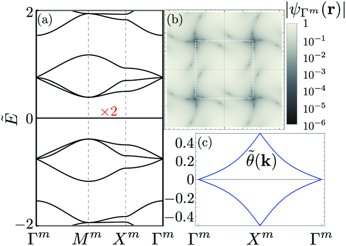
Figure 2: Four flat bands in TBG Hamiltonian under alternating magnetic field Le et al. (2022 ) .
(a), (b) Moiré unit cell and Brillouin zone, respectively.
(c) Band structure for α = 1.379 e i 0.254 π 𝛼 1.379 superscript 𝑒 𝑖 0.254 𝜋 \alpha=1.379e^{i0.254\pi} θ ~ ( 𝐤 ) = θ ( 𝐤 ) 2 π ~ 𝜃 𝐤 𝜃 𝐤 2 𝜋 \tilde{\theta}({\mathbf{k}})=\frac{\theta({\mathbf{k}})}{2\pi} | ψ K m ( 𝐫 ) | subscript 𝜓 superscript 𝐾 𝑚 𝐫 |\psi_{K^{m}}(\mathbf{r})| | ψ Γ m ( 𝐫 ) | subscript 𝜓 superscript Γ 𝑚 𝐫 |\psi_{\Gamma^{m}}(\mathbf{r})| Figure 3:
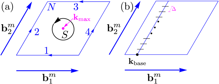
(a) Flowchart of the construction of exact flat band wave-functions starting from the wave-function at 𝐤 0 m superscript subscript 𝐤 0 𝑚 \mathbf{k}_{0}^{m} 𝐤 max subscript 𝐤 max \mathbf{k}_{\text{max}} 𝐫 0 subscript 𝐫 0 \mathbf{r}_{0} C 2 subscript 𝐶 2 C_{2}
It is important to note that the momentum 𝐤 0 m superscript subscript 𝐤 0 𝑚 \mathbf{k}_{0}^{m} 𝐤 max subscript 𝐤 max \mathbf{k}_{\text{max}} K 𝐾 K 6 ′ superscript 6 ′ 6^{\prime} 𝒞 3 z subscript 𝒞 3 𝑧 \mathcal{C}_{3z} 𝒞 2 x subscript 𝒞 2 𝑥 \mathcal{C}_{2x} 𝒞 2 z 𝒯 subscript 𝒞 2 𝑧 𝒯 \mathcal{C}_{2z}\mathcal{T} P = 𝟙 ⊗ i σ y 𝑃 tensor-product 1 𝑖 subscript 𝜎 𝑦 P=\mathds{1}\otimes i\sigma_{y} P 𝐫 = − 𝐫 𝑃 𝐫 𝐫 P\mathbf{r}=-\mathbf{r} P 𝐤 = − 𝐤 𝑃 𝐤 𝐤 P\mathbf{k}=-\mathbf{k} P ℋ ( 𝐫 ) = − ℋ ( − 𝐫 ) P 𝑃 ℋ 𝐫 ℋ 𝐫 𝑃 P\mathcal{H}(\mathbf{r})=-\mathcal{H}(-\mathbf{r})P Song et al. (2019 ); Hejazi et al. (2019 ) and chiral symmetry 𝒮 = σ z ⊗ 𝟙 𝒮 tensor-product subscript 𝜎 𝑧 1 \mathcal{S}=\sigma_{z}\otimes\mathds{1} 𝒮 𝐫 = 𝐫 𝒮 𝐫 𝐫 \mathcal{S}\mathbf{r}=\mathbf{r} 𝒮 𝐤 = 𝐤 𝒮 𝐤 𝐤 \mathcal{S}\mathbf{k}=\mathbf{k} 𝒮 ℋ ( 𝐫 ) = − ℋ ( 𝐫 ) 𝒮 𝒮 ℋ 𝐫 ℋ 𝐫 𝒮 \mathcal{S}\mathcal{H}(\mathbf{r})=-\mathcal{H}(\mathbf{r})\mathcal{S} 𝒞 2 z subscript 𝒞 2 𝑧 \mathcal{C}_{2z} 𝒞 2 z = P 𝒮 = σ z ⊗ i σ y subscript 𝒞 2 𝑧 𝑃 𝒮 tensor-product subscript 𝜎 𝑧 𝑖 subscript 𝜎 𝑦 \mathcal{C}_{2z}=P\mathcal{S}=\sigma_{z}\otimes i\sigma_{y} Wang et al. (2021b ) , and was called intra-valley inversion symmetry). As a consequence, in chiral TBG, 𝐤 max = Γ subscript 𝐤 max Γ \mathbf{k}_{\text{max}}=\Gamma 6221 ′ superscript 6221 ′ 6221^{\prime} 𝒞 3 z subscript 𝒞 3 𝑧 \mathcal{C}_{3z} 𝒞 2 z subscript 𝒞 2 𝑧 \mathcal{C}_{2z} 𝒞 2 x subscript 𝒞 2 𝑥 \mathcal{C}_{2x} 𝒯 𝒯 \mathcal{T} SM Sec. S-I for a review of symmetries of chiral TBG). In these cases, where 𝐤 0 m ≠ 𝐤 max superscript subscript 𝐤 0 𝑚 subscript 𝐤 max \mathbf{k}_{0}^{m}\neq\mathbf{k}_{\text{max}} 𝐫 0 subscript 𝐫 0 \mathbf{r}_{0} ψ 𝐤 0 m ( 𝐫 ) subscript 𝜓 superscript subscript 𝐤 0 𝑚 𝐫 \psi_{\mathbf{k}_{0}^{m}}(\mathbf{r}) ψ 𝐤 max ( 𝐫 ) = f 𝐤 max − 𝐤 0 m ( z , 𝐫 0 ) ψ 𝐤 0 m ( 𝐫 ) subscript 𝜓 subscript 𝐤 max 𝐫 subscript 𝑓 subscript 𝐤 max superscript subscript 𝐤 0 𝑚 𝑧 subscript 𝐫 0 subscript 𝜓 superscript subscript 𝐤 0 𝑚 𝐫 \psi_{\mathbf{k}_{\text{max}}}(\mathbf{r})=f_{\mathbf{k}_{\text{max}}-\mathbf{k}_{0}^{m}}(z,\mathbf{r}_{0})\psi_{\mathbf{k}_{0}^{m}}(\mathbf{r}) ψ 𝐤 max ( 𝐫 ) subscript 𝜓 subscript 𝐤 max 𝐫 \psi_{\mathbf{k}_{\text{max}}}(\mathbf{r}) ψ 𝐤 max ( 𝐫 ) subscript 𝜓 subscript 𝐤 max 𝐫 \psi_{\mathbf{k}_{\text{max}}}(\mathbf{r}) ψ 𝐤 0 m ( 𝐫 ) subscript 𝜓 superscript subscript 𝐤 0 𝑚 𝐫 \psi_{\mathbf{k}_{0}^{m}}(\mathbf{r}) Le et al. (2022 ) as is described below. The 𝐤 ⋅ 𝐩 ⋅ 𝐤 𝐩 \mathbf{k}\cdot\mathbf{p} 𝐤 0 = K subscript 𝐤 0 𝐾 \mathbf{k}_{0}=K 1
𝒟 ( 𝐫 ) = ( − 2 i ∂ z ¯ α U ( 𝐫 ) α U ( − 𝐫 ) − 2 i ∂ z ¯ ) , U ( 𝐫 ) = e − i 𝐪 1 ⋅ 𝐫 + e i ϕ e − i 𝐪 2 ⋅ 𝐫 + e − i ϕ e − i 𝐪 3 ⋅ 𝐫 , formulae-sequence 𝒟 𝐫 matrix 2 𝑖 ¯ subscript 𝑧 𝛼 𝑈 𝐫 𝛼 𝑈 𝐫 2 𝑖 ¯ subscript 𝑧 𝑈 𝐫 superscript 𝑒 ⋅ 𝑖 subscript 𝐪 1 𝐫 superscript 𝑒 𝑖 italic-ϕ superscript 𝑒 ⋅ 𝑖 subscript 𝐪 2 𝐫 superscript 𝑒 𝑖 italic-ϕ superscript 𝑒 ⋅ 𝑖 subscript 𝐪 3 𝐫 \begin{split}\mathcal{D}(\mathbf{r})&=\begin{pmatrix}-2i\overline{\partial_{z}}&\alpha U(\mathbf{r})\\
\alpha U(-\mathbf{r})&-2i\overline{\partial_{z}}\end{pmatrix},\\
U(\mathbf{r})&=e^{-i\mathbf{q}_{1}\cdot\mathbf{r}}+e^{i\phi}e^{-i\mathbf{q}_{2}\cdot\mathbf{r}}+e^{-i\phi}e^{-i\mathbf{q}_{3}\cdot\mathbf{r}},\end{split} (3)
where ϕ = 2 π 3 italic-ϕ 2 𝜋 3 \phi=\frac{2\pi}{3} 𝐪 1 = 4 π 3 a m ( 0 , − 1 ) subscript 𝐪 1 4 𝜋 3 superscript 𝑎 𝑚 0 1 \mathbf{q}_{1}=\frac{4\pi}{3a^{m}}(0,-1) 𝐪 2 , 3 = 2 π 3 a m ( ± 3 , 1 ) subscript 𝐪 2 3
2 𝜋 3 superscript 𝑎 𝑚 plus-or-minus 3 1 \mathbf{q}_{2,3}=\frac{2\pi}{3a^{m}}(\pm\sqrt{3},1) a m superscript 𝑎 𝑚 a^{m} 2 Tarnopolsky et al. (2019 ) except that here, unlike Tarnopolsky et al. (2019 ) , α 𝛼 \alpha Le et al. (2022 ) that, at certain critical complex values of α 𝛼 \alpha 2 α 𝛼 \alpha ψ 𝐤 0 m = K ( 𝐫 ) subscript 𝜓 superscript subscript 𝐤 0 𝑚 𝐾 𝐫 \psi_{\mathbf{k}_{0}^{m}=K}(\mathbf{r}) 𝐫 0 ( 1 ) = a m / 3 ( − 1 , 0 ) superscript subscript 𝐫 0 1 superscript 𝑎 𝑚 3 1 0 \mathbf{r}_{0}^{(1)}=a^{m}/\sqrt{3}(-1,0) 2 Le et al. (2022 ) how to construct the FB WFs using complex analytic function Eq. 2 ψ 𝐤 max = Γ ( 𝐫 ) = f 𝐤 max − 𝐤 0 m ( z , 𝐫 0 ( 1 ) ) ψ 𝐤 0 m ( 𝐫 ) = f 𝐪 3 ( z , 𝐫 0 ( 1 ) ) ψ K ( 𝐫 ) subscript 𝜓 subscript 𝐤 max Γ 𝐫 subscript 𝑓 subscript 𝐤 max superscript subscript 𝐤 0 𝑚 𝑧 superscript subscript 𝐫 0 1 subscript 𝜓 superscript subscript 𝐤 0 𝑚 𝐫 subscript 𝑓 subscript 𝐪 3 𝑧 superscript subscript 𝐫 0 1 subscript 𝜓 𝐾 𝐫 \psi_{\mathbf{k}_{\text{max}}=\Gamma}(\mathbf{r})=f_{\mathbf{k}_{\text{max}}-\mathbf{k}_{0}^{m}}(z,\mathbf{r}_{0}^{(1)})\psi_{\mathbf{k}_{0}^{m}}(\mathbf{r})=f_{\mathbf{q}_{3}}(z,\mathbf{r}_{0}^{(1)})\psi_{K}(\mathbf{r}) 𝐫 0 ( 1 ) = a m / 3 ( − 1 , 0 ) superscript subscript 𝐫 0 1 superscript 𝑎 𝑚 3 1 0 \mathbf{r}_{0}^{(1)}=a^{m}/\sqrt{3}(-1,0) 𝐫 0 ( 2 ) = a m / 3 ( 1 , 0 ) superscript subscript 𝐫 0 2 superscript 𝑎 𝑚 3 1 0 \mathbf{r}_{0}^{(2)}=a^{m}/\sqrt{3}(1,0) 2 𝒞 2 z = P 𝒮 subscript 𝒞 2 𝑧 𝑃 𝒮 \mathcal{C}_{2z}=P\mathcal{S} α 𝛼 \alpha 𝒞 2 x subscript 𝒞 2 𝑥 \mathcal{C}_{2x} 𝒞 6 subscript 𝒞 6 \mathcal{C}_{6} p 6 𝑝 6 p6 ψ Γ ( 𝐫 ) subscript 𝜓 Γ 𝐫 \psi_{\Gamma}(\mathbf{r}) 𝒞 2 z subscript 𝒞 2 𝑧 \mathcal{C}_{2z} 𝒞 2 z subscript 𝒞 2 𝑧 \mathcal{C}_{2z}
Ψ 𝐤 ( 1 ) ( 𝐫 ) = f 𝐤 ( z ; 𝐫 0 ( 1 ) ) f 𝐪 3 ( z , 𝐫 0 ( 1 ) ) [ ψ K ( 𝐫 ) 𝟎 ] , Ψ 𝐤 ( 2 ) ( 𝐫 ) = f 𝐤 ( z ; 𝐫 0 ( 2 ) ) f 𝐪 3 ( z , 𝐫 0 ( 1 ) ) [ ψ K ( 𝐫 ) 𝟎 ] , Ψ 𝐤 ( 3 ) ( 𝐫 ) = σ x ⊗ 𝟙 Ψ 𝒜 𝐤 ( 1 ) ∗ ( 𝒜 𝐫 ) , Ψ 𝐤 ( 4 ) ( 𝐫 ) = σ x ⊗ 𝟙 Ψ 𝒜 𝐤 ( 2 ) ∗ ( 𝒜 𝐫 ) . formulae-sequence superscript subscript Ψ 𝐤 1 𝐫 subscript 𝑓 𝐤 𝑧 superscript subscript 𝐫 0 1
subscript 𝑓 subscript 𝐪 3 𝑧 superscript subscript 𝐫 0 1 matrix subscript 𝜓 𝐾 𝐫 0 formulae-sequence superscript subscript Ψ 𝐤 2 𝐫 subscript 𝑓 𝐤 𝑧 superscript subscript 𝐫 0 2
subscript 𝑓 subscript 𝐪 3 𝑧 superscript subscript 𝐫 0 1 matrix subscript 𝜓 𝐾 𝐫 0 formulae-sequence superscript subscript Ψ 𝐤 3 𝐫 tensor-product subscript 𝜎 𝑥 1 superscript superscript subscript Ψ 𝒜 𝐤 1 𝒜 𝐫 superscript subscript Ψ 𝐤 4 𝐫 tensor-product subscript 𝜎 𝑥 1 superscript superscript subscript Ψ 𝒜 𝐤 2 𝒜 𝐫 \begin{split}\Psi_{\mathbf{k}}^{(1)}(\mathbf{r})&=f_{\mathbf{k}}(z;\mathbf{r}_{0}^{(1)})f_{\mathbf{q}_{3}}(z,\mathbf{r}_{0}^{(1)})\begin{bmatrix}\psi_{K}(\mathbf{r})\\
\mathbf{0}\end{bmatrix},\\
\Psi_{\mathbf{k}}^{(2)}(\mathbf{r})&=f_{\mathbf{k}}(z;\mathbf{r}_{0}^{(2)})f_{\mathbf{q}_{3}}(z,\mathbf{r}_{0}^{(1)})\begin{bmatrix}\psi_{K}(\mathbf{r})\\
\mathbf{0}\end{bmatrix},\\
\Psi_{\mathbf{k}}^{(3)}(\mathbf{r})&=\sigma_{x}\otimes\mathds{1}{\Psi_{\mathcal{A}\mathbf{k}}^{(1)}}^{*}(\mathcal{A}\mathbf{r}),\\
\Psi_{\mathbf{k}}^{(4)}(\mathbf{r})&=\sigma_{x}\otimes\mathds{1}{\Psi_{\mathcal{A}\mathbf{k}}^{(2)}}^{*}(\mathcal{A}\mathbf{r}).\end{split} (4)
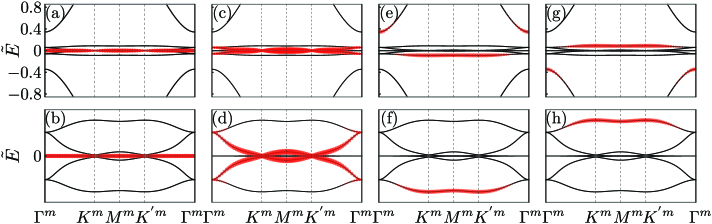
We summarize the procedure to find the number of exact FBs from the number of zeros of ψ 𝐤 max ( 𝐫 ) subscript 𝜓 subscript 𝐤 max 𝐫 \psi_{\mathbf{k}_{\text{max}}}(\mathbf{r}) 3 Bradley and Cracknell (2010 ) ) of 𝐤 max subscript 𝐤 max \mathbf{k}_{\text{max}} 3 Tarnopolsky et al. (2019 ); Le et al. (2022 ); Becker et al. (2022 , 2023 ); Wan et al. (2023 ); Eugenio and Vafek (2023 ) as well as some new ones: 2 FBs in systems with QBCP under periodic strain having p 3 𝑝 3 p3 p 4 𝑝 4 p4 p 4 𝑝 4 p4 p 4 m m 𝑝 4 𝑚 𝑚 p4mm p 4 g m 𝑝 4 𝑔 𝑚 p4gm SM SM (2 ) S-VI ), and 6 flat bands in systems with QBCP under periodic strain having p 6 m m 𝑝 6 𝑚 𝑚 p6mm 1
Construction of WFs at 𝐤 max subscript 𝐤 max \mathbf{k}_{\text{max}} 2 m 2 𝑚 2m m > 1 𝑚 1 m>1 ψ 𝐤 max subscript 𝜓 subscript 𝐤 max \psi_{\mathbf{k}_{\text{max}}} 𝐫 0 ( i ) superscript subscript 𝐫 0 𝑖 \mathbf{r}_{0}^{(i)} f 𝐤 ( z ; 𝐫 0 ( i ) ) subscript 𝑓 𝐤 𝑧 superscript subscript 𝐫 0 𝑖
f_{\mathbf{k}}(z;\mathbf{r}_{0}^{(i)}) 𝐤 𝐤 \mathbf{k} 𝐤 = 𝟎 𝐤 0 \mathbf{k}=\mathbf{0} f 𝐤 = 𝟎 ( z ; 𝐫 0 ( i ) ) = 1 subscript 𝑓 𝐤 0 𝑧 superscript subscript 𝐫 0 𝑖
1 f_{\mathbf{k}=\mathbf{0}}(z;\mathbf{r}_{0}^{(i)})=1 i = 1 , … , m 𝑖 1 … 𝑚
i=1,\dots,m 2 m 2 𝑚 2m 𝐤 ≠ 𝐤 max 𝐤 subscript 𝐤 max \mathbf{k}\neq\mathbf{k}_{\text{max}} 𝐤 max subscript 𝐤 max \mathbf{k}_{\text{max}} 2 ( m − 1 ) 2 𝑚 1 2(m-1) 𝐤 max subscript 𝐤 max \mathbf{k}_{\text{max}} ψ 𝐤 + 𝐤 max ( i ) ( 𝐫 ) = f 𝐤 ( z ; 𝐫 0 ( i ) ) ψ 𝐤 max ( 𝐫 ) superscript subscript 𝜓 𝐤 subscript 𝐤 max 𝑖 𝐫 subscript 𝑓 𝐤 𝑧 superscript subscript 𝐫 0 𝑖
subscript 𝜓 subscript 𝐤 max 𝐫 \psi_{\mathbf{k}+\mathbf{k}_{\text{max}}}^{(i)}(\mathbf{r})=f_{\mathbf{k}}(z;\mathbf{r}_{0}^{(i)})\psi_{\mathbf{k}_{\text{max}}}(\mathbf{r}) 𝐤 ≠ 𝐤 max 𝐤 subscript 𝐤 max \mathbf{k}\neq\mathbf{k}_{\text{max}} ( m − 1 ) 𝑚 1 (m-1) ψ 𝐤 ( 1 ) ( 𝐫 ) superscript subscript 𝜓 𝐤 1 𝐫 \psi_{\mathbf{k}}^{(1)}(\mathbf{r})
ψ ~ 𝐤 ( i ) ( 𝐫 ) = { ψ 𝐤 ( 1 ) ( 𝐫 ) if i = 1 , ψ 𝐤 ( i ) ( 𝐫 ) − ⟨ ψ 𝐤 ( 1 ) | ψ 𝐤 ( i ) ⟩ ⟨ ψ 𝐤 ( 1 ) | ψ 𝐤 ( 1 ) ⟩ ψ 𝐤 ( 1 ) ( 𝐫 ) if i ≠ 1 , superscript subscript ~ 𝜓 𝐤 𝑖 𝐫 cases superscript subscript 𝜓 𝐤 1 𝐫 if 𝑖 1 superscript subscript 𝜓 𝐤 𝑖 𝐫 inner-product superscript subscript 𝜓 𝐤 1 superscript subscript 𝜓 𝐤 𝑖 inner-product superscript subscript 𝜓 𝐤 1 superscript subscript 𝜓 𝐤 1 superscript subscript 𝜓 𝐤 1 𝐫 if 𝑖 1 \tilde{\psi}_{\mathbf{k}}^{(i)}(\mathbf{r})=\begin{cases}\psi_{\mathbf{k}}^{(1)}(\mathbf{r})&\text{ if }i=1,\\
\psi_{\mathbf{k}}^{(i)}(\mathbf{r})-\frac{\langle\psi_{\mathbf{k}}^{(1)}|\psi_{\mathbf{k}}^{(i)}\rangle}{\langle\psi_{\mathbf{k}}^{(1)}|\psi_{\mathbf{k}}^{(1)}\rangle}\psi_{\mathbf{k}}^{(1)}(\mathbf{r})&\text{ if }i\neq 1,\\
\end{cases} (5)
where ⟨ f | g ⟩ = ∫ unit cell d 2 𝐫 f ∗ ( 𝐫 ) g ( 𝐫 ) inner-product 𝑓 𝑔 subscript unit cell superscript 𝑑 2 𝐫 superscript 𝑓 𝐫 𝑔 𝐫 \langle f|g\rangle=\int_{\text{unit cell}}d^{2}\mathbf{r}f^{*}(\mathbf{r})g(\mathbf{r}) f 𝐤 ( z ; 𝐫 0 ) subscript 𝑓 𝐤 𝑧 subscript 𝐫 0
f_{\mathbf{k}}(z;\mathbf{r}_{0}) f ~ 𝐤 ( 𝐫 ; 𝐫 0 ) subscript ~ 𝑓 𝐤 𝐫 subscript 𝐫 0
\tilde{f}_{\mathbf{k}}(\mathbf{r};\mathbf{r}_{0})
of k = k x + i k y 𝑘 subscript 𝑘 𝑥 𝑖 subscript 𝑘 𝑦 k=k_{x}+ik_{y} e i 𝐤 ⋅ 𝐫 superscript 𝑒 ⋅ 𝑖 𝐤 𝐫 e^{i\mathbf{k}\cdot\mathbf{r}} f ~ 𝟎 ( 𝐫 ; 𝐫 0 ) = 1 subscript ~ 𝑓 0 𝐫 subscript 𝐫 0
1 \tilde{f}_{\mathbf{0}}(\mathbf{r};\mathbf{r}_{0})=1 f 𝐤 ( z , 𝐫 0 ) = 1 + f ~ 𝟎 ′ ( 𝐫 ; 𝐫 0 ) k + i ( k z ∗ + k ∗ z ) / 2 + 𝒪 ( k 2 ) subscript 𝑓 𝐤 𝑧 subscript 𝐫 0 1 superscript subscript ~ 𝑓 0 ′ 𝐫 subscript 𝐫 0
𝑘 𝑖 𝑘 superscript 𝑧 superscript 𝑘 𝑧 2 𝒪 superscript 𝑘 2 f_{\mathbf{k}}(z,\mathbf{r}_{0})=1+\tilde{f}_{\mathbf{0}}^{\prime}(\mathbf{r};\mathbf{r}_{0})k+i(kz^{*}+k^{*}z)/2+\mathcal{O}(k^{2}) f ~ 𝟎 ′ ( 𝐫 ; 𝐫 0 ) ≡ 1 2 [ ( ∂ k x − i ∂ k y ) f ~ 𝐤 ( 𝐫 ; 𝐫 0 ) ] | 𝐤 = 𝟎 superscript subscript ~ 𝑓 0 ′ 𝐫 subscript 𝐫 0
evaluated-at 1 2 delimited-[] subscript subscript 𝑘 𝑥 𝑖 subscript subscript 𝑘 𝑦 subscript ~ 𝑓 𝐤 𝐫 subscript 𝐫 0
𝐤 0 \tilde{f}_{\mathbf{0}}^{\prime}(\mathbf{r};\mathbf{r}_{0})\equiv\frac{1}{2}[(\partial_{k_{x}}-i\partial_{k_{y}})\tilde{f}_{\mathbf{k}}(\mathbf{r};\mathbf{r}_{0})]|_{\mathbf{k}=\mathbf{0}} 5 𝐤 max subscript 𝐤 max \mathbf{k}_{\text{max}}
ψ ~ 𝐤 max + 𝐤 ( i ) ( 𝐫 ) ≈ { ( 1 + k f ~ 𝟎 ′ ( 𝐫 ; 𝐫 0 ( 1 ) ) + ( k z ∗ + k ∗ z ) / 2 ) ψ 𝐤 max ( 𝐫 ) if i = 1 , k ( f ~ 𝟎 ′ ( 𝐫 ; 𝐫 0 ( i ) ) − f ~ 𝟎 ′ ( 𝐫 ; 𝐫 0 ( 1 ) ) − ⟨ ψ 𝐤 max | ( f ~ 𝟎 ′ ( 𝐫 ; 𝐫 0 ( i ) ) − f ~ 𝟎 ′ ( 𝐫 ; 𝐫 0 ( 1 ) ) ) ψ 𝐤 max ⟩ ) ψ 𝐤 max ( 𝐫 ) if i ≠ 1 . superscript subscript ~ 𝜓 subscript 𝐤 max 𝐤 𝑖 𝐫 cases 1 𝑘 superscript subscript ~ 𝑓 0 ′ 𝐫 superscript subscript 𝐫 0 1
𝑘 superscript 𝑧 superscript 𝑘 𝑧 2 subscript 𝜓 subscript 𝐤 max 𝐫 if 𝑖 1 𝑘 superscript subscript ~ 𝑓 0 ′ 𝐫 superscript subscript 𝐫 0 𝑖
superscript subscript ~ 𝑓 0 ′ 𝐫 superscript subscript 𝐫 0 1
inner-product subscript 𝜓 subscript 𝐤 max superscript subscript ~ 𝑓 0 ′ 𝐫 superscript subscript 𝐫 0 𝑖
superscript subscript ~ 𝑓 0 ′ 𝐫 superscript subscript 𝐫 0 1
subscript 𝜓 subscript 𝐤 max subscript 𝜓 subscript 𝐤 max 𝐫 if 𝑖 1 \tilde{\psi}_{\mathbf{k}_{\text{max}}+\mathbf{k}}^{(i)}(\mathbf{r})\approx\begin{cases}(1+k\tilde{f}_{\mathbf{0}}^{\prime}(\mathbf{r};\mathbf{r}_{0}^{(1)})+(kz^{*}+k^{*}z)/2)\psi_{\mathbf{k}_{\text{max}}}(\mathbf{r})&\text{ if }i=1,\\
k(\tilde{f}_{\mathbf{0}}^{\prime}(\mathbf{r};\mathbf{r}_{0}^{(i)})-\tilde{f}_{\mathbf{0}}^{\prime}(\mathbf{r};\mathbf{r}_{0}^{(1)})-\langle\psi_{\mathbf{k}_{\text{max}}}|(\tilde{f}_{\mathbf{0}}^{\prime}(\mathbf{r};\mathbf{r}_{0}^{(i)})-\tilde{f}_{\mathbf{0}}^{\prime}(\mathbf{r};\mathbf{r}_{0}^{(1)}))\psi_{\mathbf{k}_{\text{max}}}\rangle)\psi_{\mathbf{k}_{\text{max}}}(\mathbf{r})&\text{ if }i\neq 1.\\
\end{cases} (6)
Continuing these WFs to 𝐤 max subscript 𝐤 max \mathbf{k}_{\text{max}}
ψ ~ 𝐤 max ( i ) ( 𝐫 ) = { ψ 𝐤 max ( 𝐫 ) if i = 1 , ( f ~ 𝟎 ′ ( 𝐫 ; 𝐫 0 ( i ) ) − f ~ 𝟎 ′ ( 𝐫 ; 𝐫 0 ( 1 ) ) − ⟨ ψ 𝐤 max | ( f ~ 𝟎 ′ ( 𝐫 ; 𝐫 0 ( i ) ) − f ~ 𝟎 ′ ( 𝐫 ; 𝐫 0 ( 1 ) ) ) ψ 𝐤 max ⟩ ) ψ 𝐤 max ( 𝐫 ) if i ≠ 1 . superscript subscript ~ 𝜓 subscript 𝐤 max 𝑖 𝐫 cases subscript 𝜓 subscript 𝐤 max 𝐫 if 𝑖 1 superscript subscript ~ 𝑓 0 ′ 𝐫 superscript subscript 𝐫 0 𝑖
superscript subscript ~ 𝑓 0 ′ 𝐫 superscript subscript 𝐫 0 1
inner-product subscript 𝜓 subscript 𝐤 max superscript subscript ~ 𝑓 0 ′ 𝐫 superscript subscript 𝐫 0 𝑖
superscript subscript ~ 𝑓 0 ′ 𝐫 superscript subscript 𝐫 0 1
subscript 𝜓 subscript 𝐤 max subscript 𝜓 subscript 𝐤 max 𝐫 if 𝑖 1 \tilde{\psi}_{\mathbf{k}_{\text{max}}}^{(i)}(\mathbf{r})=\begin{cases}\psi_{\mathbf{k}_{\text{max}}}(\mathbf{r})&\text{ if }i=1,\\
(\tilde{f}_{\mathbf{0}}^{\prime}(\mathbf{r};\mathbf{r}_{0}^{(i)})-\tilde{f}_{\mathbf{0}}^{\prime}(\mathbf{r};\mathbf{r}_{0}^{(1)})-\langle\psi_{\mathbf{k}_{\text{max}}}|(\tilde{f}_{\mathbf{0}}^{\prime}(\mathbf{r};\mathbf{r}_{0}^{(i)})-\tilde{f}_{\mathbf{0}}^{\prime}(\mathbf{r};\mathbf{r}_{0}^{(1)}))\psi_{\mathbf{k}_{\text{max}}}\rangle)\psi_{\mathbf{k}_{\text{max}}}(\mathbf{r})&\text{ if }i\neq 1.\\
\end{cases} (7)
Note that f ~ 𝟎 ′ ( 𝐫 ; 𝐫 0 ( i ) ) − f ~ 𝟎 ′ ( 𝐫 ; 𝐫 0 ( 1 ) ) superscript subscript ~ 𝑓 0 ′ 𝐫 superscript subscript 𝐫 0 𝑖
superscript subscript ~ 𝑓 0 ′ 𝐫 superscript subscript 𝐫 0 1
\tilde{f}_{\mathbf{0}}^{\prime}(\mathbf{r};\mathbf{r}_{0}^{(i)})-\tilde{f}_{\mathbf{0}}^{\prime}(\mathbf{r};\mathbf{r}_{0}^{(1)}) z = x + i y 𝑧 𝑥 𝑖 𝑦 z=x+iy f ~ 𝐤 ( 𝐫 ; 𝐫 0 ) subscript ~ 𝑓 𝐤 𝐫 subscript 𝐫 0
\tilde{f}_{\mathbf{k}}(\mathbf{r};\mathbf{r}_{0})
is not holomorphic, hence ψ ~ 𝐤 max ( i ) ( 𝐫 ) superscript subscript ~ 𝜓 subscript 𝐤 max 𝑖 𝐫 \tilde{\psi}_{\mathbf{k}_{\text{max}}}^{(i)}(\mathbf{r}) 𝒟 ( 𝐫 ) ψ ~ 𝐤 max ( i ) ( 𝐫 ) = 𝟎 𝒟 𝐫 superscript subscript ~ 𝜓 subscript 𝐤 max 𝑖 𝐫 0 \mathcal{D}(\mathbf{r})\tilde{\psi}_{\mathbf{k}_{\text{max}}}^{(i)}(\mathbf{r})=\mathbf{0} ( m − 1 ) 𝑚 1 (m-1) 𝐤 max subscript 𝐤 max \mathbf{k}_{\text{max}} ψ 𝐤 max ( 𝐫 ) subscript 𝜓 subscript 𝐤 max 𝐫 \psi_{\mathbf{k}_{\text{max}}}(\mathbf{r}) m 𝑚 m 𝐤 max subscript 𝐤 max \mathbf{k}_{\text{max}} ( ψ ~ 𝐤 max ( i ) ( 𝒜 𝐫 ) ) ∗ superscript superscript subscript ~ 𝜓 subscript 𝐤 max 𝑖 𝒜 𝐫 (\tilde{\psi}_{\mathbf{k}_{\text{max}}}^{(i)}(\mathcal{A}\mathbf{r}))^{*} 𝐤 max = Γ subscript 𝐤 max Γ \mathbf{k}_{\text{max}}=\Gamma see SM SM (2 ) S-III for details ).
Co-dimension of the tuning parameters. –Since ψ 𝐤 max ( 𝐫 ) subscript 𝜓 subscript 𝐤 max 𝐫 \psi_{\mathbf{k}_{\text{max}}}(\mathbf{r}) l 𝑙 l l 𝑙 l ψ 𝐤 max ( 𝐫 0 ) = 𝟎 subscript 𝜓 subscript 𝐤 max subscript 𝐫 0 0 \psi_{\mathbf{k}_{\text{max}}}(\mathbf{r}_{0})=\mathbf{0} 2 l 2 𝑙 2l 2 l 2 𝑙 2l 2 l 2 𝑙 2l ψ 𝐤 max ( 𝐫 ) subscript 𝜓 subscript 𝐤 max 𝐫 \psi_{\mathbf{k}_{\text{max}}}(\mathbf{r}) 𝒞 3 z subscript 𝒞 3 𝑧 \mathcal{C}_{3z} Tarnopolsky et al. (2019 ) , also SM SM (2 ) S-II for details), in all cases, that we are considering, the co-dimension is 2, unless there are extra symmetries. If the HSP 𝐫 0 subscript 𝐫 0 \mathbf{r}_{0} ℳ ℳ \mathcal{M} ℳ 𝒜 ℳ 𝒜 \mathcal{M}\mathcal{A} ± 1 plus-or-minus 1 \pm 1 𝒞 n z subscript 𝒞 𝑛 𝑧 \mathcal{C}_{nz} n ≥ 3 𝑛 3 n\geq 3 𝒜 𝒜 \mathcal{A} σ x ⊗ 𝟙 𝒦 tensor-product subscript 𝜎 𝑥 1 𝒦 \sigma_{x}\otimes\mathds{1}\mathcal{K} ℳ 2 = 𝟙 superscript ℳ 2 1 \mathcal{M}^{2}=\mathds{1} C 2 x subscript 𝐶 2 𝑥 C_{2x} ψ 𝐤 max ( 𝐫 ) subscript 𝜓 subscript 𝐤 max 𝐫 \psi_{\mathbf{k}_{\text{max}}}(\mathbf{r}) 𝐫 = 𝐫 0 𝐫 subscript 𝐫 0 \mathbf{r}=\mathbf{r}_{0} ρ ( ℳ ) = σ x 𝜌 ℳ subscript 𝜎 𝑥 \rho(\mathcal{M})=\sigma_{x} ℳ 𝒜 ℳ 𝒜 \mathcal{MA} P 𝒮 𝒞 2 x 𝒞 2 z 𝒯 𝑃 𝒮 subscript 𝒞 2 𝑥 subscript 𝒞 2 𝑧 𝒯 P\mathcal{S}\mathcal{C}_{2x}\mathcal{C}_{2z}\mathcal{T} P 𝒮 𝒞 2 x 𝒞 2 z 𝒯 ( x , y ) = ( x , − y ) 𝑃 𝒮 subscript 𝒞 2 𝑥 subscript 𝒞 2 𝑧 𝒯 𝑥 𝑦 𝑥 𝑦 P\mathcal{S}\mathcal{C}_{2x}\mathcal{C}_{2z}\mathcal{T}(x,y)=(x,-y) P 𝒮 𝒞 2 x 𝒞 2 z 𝒯 ( k x , k y ) = ( − k x , k y ) 𝑃 𝒮 subscript 𝒞 2 𝑥 subscript 𝒞 2 𝑧 𝒯 subscript 𝑘 𝑥 subscript 𝑘 𝑦 subscript 𝑘 𝑥 subscript 𝑘 𝑦 P\mathcal{S}\mathcal{C}_{2x}\mathcal{C}_{2z}\mathcal{T}(k_{x},k_{y})=(-k_{x},k_{y}) K m superscript 𝐾 𝑚 K^{m} ρ ( P 𝒮 𝒞 2 x 𝒞 2 z 𝒯 ) = σ z ⊗ σ z 𝒦 𝜌 𝑃 𝒮 subscript 𝒞 2 𝑥 subscript 𝒞 2 𝑧 𝒯 tensor-product subscript 𝜎 𝑧 subscript 𝜎 𝑧 𝒦 \rho(P\mathcal{S}\mathcal{C}_{2x}\mathcal{C}_{2z}\mathcal{T})=\sigma_{z}\otimes\sigma_{z}\mathcal{K} Le et al. (2022 ) , 𝒞 2 x subscript 𝒞 2 𝑥 \mathcal{C}_{2x} 3 Sheffer et al. (2023 ) .
Topology and quantum geometry of the FBs. –As was mentioned earlier, it can be proven that the sublattice polarized exact FB WFs have Chern number C = ± 1 𝐶 plus-or-minus 1 C=\pm 1 k 𝑘 k see SM SM (2 ) S-IV for details ), for the case where there are only two FBs, have ± 1 plus-or-minus 1 \pm 1 1 ± 1 plus-or-minus 1 \pm 1 1 2 m 𝑚 m | C | = 1 𝐶 1 |C|=1 | C | = m 𝐶 𝑚 |C|=m ψ 𝐤 + 𝐤 max ( i ) ( 𝐫 ) = f 𝐤 ( z ; 𝐫 0 ( i ) ) ψ 𝐤 max ( 𝐫 ) superscript subscript 𝜓 𝐤 subscript 𝐤 max 𝑖 𝐫 subscript 𝑓 𝐤 𝑧 superscript subscript 𝐫 0 𝑖
subscript 𝜓 subscript 𝐤 max 𝐫 \psi_{\mathbf{k}+\mathbf{k}_{\text{max}}}^{(i)}(\mathbf{r})=f_{\mathbf{k}}(z;\mathbf{r}_{0}^{(i)})\psi_{\mathbf{k}_{\text{max}}}(\mathbf{r}) 5 m − 1 𝑚 1 m-1 k 𝑘 k 𝐤 = 0 𝐤 0 \mathbf{k}=0 6 𝐤 = 0 𝐤 0 \mathbf{k}=0 C = 0 𝐶 0 C=0 see SM SM (2 ) S-IV for details ). As a consequence, only one of the sublattice polarized WFs carry | C | = 1 𝐶 1 |C|=1 Song et al. (2021 ) , where it was shown that for systems with an antiunitary particle-hole symmetry 𝒫 𝒫 \mathcal{P} 𝒫 2 = − 𝟙 superscript 𝒫 2 1 \mathcal{P}^{2}=-\mathds{1} 4 p + 2 4 𝑝 2 4p+2 p ∈ ℕ 𝑝 ℕ p\in\mathds{N} ℤ 2 subscript ℤ 2 \mathds{Z}_{2} C = ± 1 𝐶 plus-or-minus 1 C=\pm 1 𝒫 𝒫 \mathcal{P} 𝒫 = 𝒮 𝒯 𝒫 𝒮 𝒯 \mathcal{P}=\mathcal{S}\mathcal{T} 𝒫 = P 𝒞 2 z 𝒯 𝒫 𝑃 subscript 𝒞 2 𝑧 𝒯 \mathcal{P}=P\mathcal{C}_{2z}\mathcal{T} Li et al. (2022 ) has 2 FBs with Chern numbers ± 2 plus-or-minus 2 \pm 2 p 4 m m 𝑝 4 𝑚 𝑚 p4mm see SM SM (2 ) S-VII for details ). Also, if one replaces the p 4 m m 𝑝 4 𝑚 𝑚 p4mm p 4 g m 𝑝 4 𝑔 𝑚 p4gm C = ± 2 𝐶 plus-or-minus 2 C=\pm 2 see SM SM (2 ) S-VII ); this doubling of number of FBs in p 4 g m 𝑝 4 𝑔 𝑚 p4gm Dresselhaus et al. (2008 ) . We further show in the SM SM (2 ) S-V , that the FBs with higher degeneracy satisfy ideal non-Abelian trace condition: tr ( g α β m n ( 𝐤 ) ) = ∑ n ′ ∑ α ∈ { x , y } g α α n n ( 𝐤 ) = | tr ( F x y m n ( 𝐤 ) ) | = | ∑ n ′ F x y n n ( 𝐤 ) | tr subscript superscript 𝑔 𝑚 𝑛 𝛼 𝛽 𝐤 superscript subscript 𝑛 ′ subscript 𝛼 𝑥 𝑦 subscript superscript 𝑔 𝑛 𝑛 𝛼 𝛼 𝐤 tr superscript subscript 𝐹 𝑥 𝑦 𝑚 𝑛 𝐤 superscript subscript 𝑛 ′ superscript subscript 𝐹 𝑥 𝑦 𝑛 𝑛 𝐤 \text{tr}(g^{mn}_{\alpha\beta}(\mathbf{k}))=\sum_{n}^{\prime}\sum_{\alpha\in\{x,y\}}g^{nn}_{\alpha\alpha}(\mathbf{k})=|\text{tr}(F_{xy}^{mn}(\mathbf{k}))|=|\sum_{n}^{\prime}F_{xy}^{nn}(\mathbf{k})| g i j m n ( 𝐤 ) superscript subscript 𝑔 𝑖 𝑗 𝑚 𝑛 𝐤 g_{ij}^{mn}(\mathbf{k}) F x y m n ( 𝐤 ) superscript subscript 𝐹 𝑥 𝑦 𝑚 𝑛 𝐤 F_{xy}^{mn}(\mathbf{k}) n 𝑛 n
Figure 4: Topological heavy fermion model for the system with 6 flat bands in Fig. 1 α ~ = 2.53 ~ 𝛼 2.53 \tilde{\alpha}=2.53 α ~ = 2.93 ~ 𝛼 2.93 \tilde{\alpha}=2.93 E ~ ∈ ( − 0.4 , 0.4 ) ~ 𝐸 0.4 0.4 \tilde{E}\in(-0.4,0.4) Ω ( 𝐤 n ) Ω subscript 𝐤 𝑛 \Omega(\mathbf{k}_{n})
Topological heavy fermion (THF) model. –Due to the antiunitary particle-hole symmetry 𝒫 𝒫 \mathcal{P} Song et al. (2021 ) . As a consequence, a tight binding description of these bands is never possible. However, in the case of TBG, due to the fact that the Berry curvature distribution is peaked at Γ Γ \Gamma Song and Bernevig (2022 ) that hybridization of 2 atomic limit HF bands with 4 topological conduction bands (having nontrivial winding) at Γ Γ \Gamma 4 G = p 6 m m 𝐺 𝑝 6 𝑚 𝑚 G=p6mm 1 Γ 5 ⊕ 2 Γ 6 − 2 M 1 ⊕ 2 M 2 ⊕ M 3 ⊕ M 4 − K 1 ⊕ K 2 ⊕ 2 K 3 direct-sum direct-sum direct-sum subscript Γ 5 2 subscript Γ 6 2 subscript 𝑀 1 2 subscript 𝑀 2 subscript 𝑀 3 subscript 𝑀 4 subscript 𝐾 1 subscript 𝐾 2 2 subscript 𝐾 3 \Gamma_{5}\oplus 2\Gamma_{6}-2M_{1}\oplus 2M_{2}\oplus M_{3}\oplus M_{4}-K_{1}\oplus K_{2}\oplus 2K_{3} Bradlyn et al. (2017 ) . On the other hand, the two lowest higher energy bands have representations Γ 1 subscript Γ 1 \Gamma_{1} Γ 2 subscript Γ 2 \Gamma_{2} Γ Γ \Gamma Γ 6 subscript Γ 6 \Gamma_{6} Γ 1 ⊕ Γ 2 direct-sum subscript Γ 1 subscript Γ 2 \Gamma_{1}\oplus\Gamma_{2} B R = ( A 1 ↑ G ) 1 a ⊕ ( A 2 ↑ G ) 1 a ⊕ ( E 1 ↑ G ) 1 a ⊕ ( E 2 ↑ G ) 1 a 𝐵 𝑅 direct-sum subscript ↑ subscript 𝐴 1 𝐺 1 𝑎 subscript ↑ subscript 𝐴 2 𝐺 1 𝑎 subscript ↑ subscript 𝐸 1 𝐺 1 𝑎 subscript ↑ subscript 𝐸 2 𝐺 1 𝑎 BR=(A_{1}\uparrow G)_{1a}\oplus(A_{2}\uparrow G)_{1a}\oplus(E_{1}\uparrow G)_{1a}\oplus(E_{2}\uparrow G)_{1a} Aroyo et al. (2011 , 2006a , 2006b ) . This and the fact that the Berry curvature distribution of the 6 FBs being peaked at Γ Γ \Gamma 4 B R 𝐵 𝑅 BR c 𝑐 c Γ 6 subscript Γ 6 \Gamma_{6} A 1 subscript 𝐴 1 A_{1} A 2 subscript 𝐴 2 A_{2} E 1 subscript 𝐸 1 E_{1} E 2 subscript 𝐸 2 E_{2} C 6 v subscript 𝐶 6 𝑣 C_{6v} 4 Γ Γ \Gamma A 1 subscript 𝐴 1 A_{1} A 2 subscript 𝐴 2 A_{2} f 𝑓 f Marzari and Vanderbilt (1997 ); Souza et al. (2001 ); Pizzi et al. (2020 ) (see SM SM (2 ) S-VIII for details ), these MLWFs are extremely localized as can be seen in Fig. 4 f 𝑓 f c 𝑐 c
ℋ ^ = ∑ | 𝐤 | < Λ c H a b ( c ) ( 𝐤 ) c a † ( 𝐤 ) c b ( 𝐤 ) + ∑ 𝐑 H α β ( f ) f α † ( 𝐑 ) f β ( 𝐑 ) + ^ ℋ subscript 𝐤 subscript Λ 𝑐 subscript superscript 𝐻 𝑐 𝑎 𝑏 𝐤 subscript superscript 𝑐 † 𝑎 𝐤 subscript 𝑐 𝑏 𝐤 limit-from subscript 𝐑 subscript superscript 𝐻 𝑓 𝛼 𝛽 subscript superscript 𝑓 † 𝛼 𝐑 subscript 𝑓 𝛽 𝐑 \displaystyle\hat{\mathcal{H}}=\sum_{|\mathbf{k}|<\Lambda_{c}}H^{(c)}_{ab}(\mathbf{k})c^{\dagger}_{a}(\mathbf{k})c_{b}(\mathbf{k})+\sum_{\mathbf{R}}H^{(f)}_{\alpha\beta}f^{\dagger}_{\alpha}(\mathbf{R})f_{\beta}(\mathbf{R})+
∑ | 𝐤 | < Λ c , 𝐑 ( H a α ( c f ) ( 𝐤 ) e − i 𝐤 ⋅ 𝐑 − | 𝐤 | 2 λ 2 / 2 c a † ( 𝐤 ) f α ( 𝐑 ) + h.c. ) , subscript 𝐤 subscript Λ 𝑐 𝐑
subscript superscript 𝐻 𝑐 𝑓 𝑎 𝛼 𝐤 superscript 𝑒 ⋅ 𝑖 𝐤 𝐑 superscript 𝐤 2 superscript 𝜆 2 2 subscript superscript 𝑐 † 𝑎 𝐤 subscript 𝑓 𝛼 𝐑 h.c. \displaystyle\phantom{\hat{\mathcal{H}}}\sum_{|\mathbf{k}|<\Lambda_{c},\mathbf{R}}\left(H^{(cf)}_{a\alpha}(\mathbf{k})e^{-i\mathbf{k}\cdot\mathbf{R}-|\mathbf{k}|^{2}\lambda^{2}/2}c^{\dagger}_{a}(\mathbf{k})f_{\alpha}(\mathbf{R})+\text{h.c.}\right),
H ( c ) ( 𝐤 ) ≈ c 1 ( k x 2 − k y 2 ) σ x − 2 c 1 k x k y σ y , superscript 𝐻 𝑐 𝐤 subscript 𝑐 1 superscript subscript 𝑘 𝑥 2 superscript subscript 𝑘 𝑦 2 subscript 𝜎 𝑥 2 subscript 𝑐 1 subscript 𝑘 𝑥 subscript 𝑘 𝑦 subscript 𝜎 𝑦 \displaystyle H^{(c)}(\mathbf{k})\approx c_{1}(k_{x}^{2}-k_{y}^{2})\sigma_{x}-2c_{1}k_{x}k_{y}\sigma_{y},
H ( f ) ≈ ( m σ z 𝟎 2 × 4 𝟎 4 × 2 𝟎 4 × 4 ) , superscript 𝐻 𝑓 matrix 𝑚 subscript 𝜎 𝑧 subscript 0 2 4 subscript 0 4 2 subscript 0 4 4 \displaystyle H^{(f)}\approx\begin{pmatrix}m\sigma_{z}&\mathbf{0}_{2\times 4}\\
\mathbf{0}_{4\times 2}&\mathbf{0}_{4\times 4}\end{pmatrix},
H ( c f ) ( 𝐤 ) ≈ ( − i c 2 ( k x − i k y ) c 2 ( k x − i k y ) 0 γ 0 0 − i c 2 ( k x + i k y ) − c 2 ( k x + i k y ) γ 0 0 0 ) superscript 𝐻 𝑐 𝑓 𝐤 matrix 𝑖 subscript 𝑐 2 subscript 𝑘 𝑥 𝑖 subscript 𝑘 𝑦 subscript 𝑐 2 subscript 𝑘 𝑥 𝑖 subscript 𝑘 𝑦 0 𝛾 0 0 𝑖 subscript 𝑐 2 subscript 𝑘 𝑥 𝑖 subscript 𝑘 𝑦 subscript 𝑐 2 subscript 𝑘 𝑥 𝑖 subscript 𝑘 𝑦 𝛾 0 0 0 \displaystyle H^{(cf)}(\mathbf{k})\approx\begin{pmatrix}-ic_{2}(k_{x}-ik_{y})&c_{2}(k_{x}-ik_{y})&0&\gamma&0&0\\
-ic_{2}(k_{x}+ik_{y})&-c_{2}(k_{x}+ik_{y})&\gamma&0&0&0\\
\end{pmatrix} (8)
where α ∈ { A 1 , A 2 , E 1 1 , E 1 2 , E 2 1 , E 2 2 } 𝛼 subscript 𝐴 1 subscript 𝐴 2 superscript subscript 𝐸 1 1 superscript subscript 𝐸 1 2 superscript subscript 𝐸 2 1 superscript subscript 𝐸 2 2 \alpha\in\{A_{1},A_{2},E_{1}^{1},E_{1}^{2},E_{2}^{1},E_{2}^{2}\} f 𝑓 f m 𝑚 m γ 𝛾 \gamma Γ 1 subscript Γ 1 \Gamma_{1} Γ 2 subscript Γ 2 \Gamma_{2} Γ 6 subscript Γ 6 \Gamma_{6} Γ 6 subscript Γ 6 \Gamma_{6} 4 c 1 subscript 𝑐 1 c_{1} c 2 subscript 𝑐 2 c_{2} ℋ ^ ^ ℋ \hat{\mathcal{H}} 4
Conclusion. –In this letter, we systematically studied single and bilayer continuum Hamiltonians under moiré periodic modulations, and classified all possible number of exact flat bands that can appear in systems with different point group symmetries, and examined their topology. We not only showed that all single and bilayer systems in literature (to our knowledge) fall into this classification, but also found several new examples of model systems that can host high number of flat bands as well as high Chern number. In the future, it would be interesting to study the interplay between interactions and high number of flat bands that can enrich the correlated states in these systems.
Acknowledgements .–This work was supported in part by Air Force Office of Scientific Research MURI FA9550-23-1-0334 and the Office of Naval Research MURI N00014-20-1-2479 (XW, SS and KS) and Award N00014-21-1-2770 (XW and KS), and by the Gordon and Betty Moore Foundation Award N031710 (KS). The work at LANL (SZL) was carried out under the auspices of the U.S. DOE NNSA under contract No. 89233218CNA000001 through the LDRD Program, and was supported by the Center for Nonlinear Studies at LANL, and was performed, in part, at the Center for Integrated Nanotechnologies, an Office of Science User Facility operated for the U.S. DOE Office of Science, under user proposals # 2018 B U 0010 # 2018 𝐵 𝑈 0010 \#2018BU0010 # 2018 B U 0083 # 2018 𝐵 𝑈 0083 \#2018BU0083
References
Tarnopolsky et al. (2019)
G. Tarnopolsky, A. J. Kruchkov, and A. Vishwanath, Physical review letters 122 , 106405 (2019).
Haldane and Rezayi (1985)
F. D. M. Haldane and E. H. Rezayi, Physical Review B 31 , 2529 (1985).
Li et al. (2022)
M.-R. Li, A.-L. He, and H. Yao, Physical Review Research 4 , 043151 (2022).
Becker et al. (2022)
S. Becker, T. Humbert, and M. Zworski, arXiv preprint
arXiv:2208.01628 (2022).
Le et al. (2022)
C. Le, Q. Zhang, C. Fan, X. Wu, and C.-K. Chiu, arXiv preprint arXiv:2210.13976 (2022).
Wan et al. (2023)
X. Wan, S. Sarkar,
S.-Z. Lin, and K. Sun, Physical Review Letters 130 , 216401 (2023).
Eugenio and Vafek (2023)
P. M. Eugenio and O. Vafek, SciPost
Physics 15 , 081
(2023).
Becker et al. (2023)
S. Becker, T. Humbert, and M. Zworski, arXiv preprint
arXiv:2306.02909 (2023).
Neupert et al. (2011)
T. Neupert, L. Santos,
C. Chamon, and C. Mudry, Physical review letters 106 , 236804 (2011).
Qi (2011)
X.-L. Qi, Physical
review letters 107 , 126803 (2011).
Wang and Ran (2011)
F. Wang and Y. Ran, Physical Review
B 84 , 241103 (2011).
Wang et al. (2012)
Y.-F. Wang, H. Yao, C.-D. Gong, and D. Sheng, Physical Review B 86 , 201101 (2012).
Yang et al. (2012)
S. Yang, Z.-C. Gu,
K. Sun, and S. D. Sarma, Physical Review B 86 , 241112 (2012).
Wu et al. (2013)
Y.-L. Wu, N. Regnault, and B. A. Bernevig, Physical review
letters 110 , 106802
(2013).
Andrews and Soluyanov (2020)
B. Andrews and A. Soluyanov, Physical Review B 101 , 235312 (2020).
Liu et al. (2021)
Z. Liu, A. Abouelkomsan, and E. J. Bergholtz, Physical Review
Letters 126 , 026801
(2021).
Andrews et al. (2021)
B. Andrews, T. Neupert, and G. Möller, Physical Review
B 104 , 125107 (2021).
Zhang et al. (2019)
Y.-H. Zhang, D. Mao, Y. Cao, P. Jarillo-Herrero, and T. Senthil, Physical Review B 99 , 075127 (2019).
SM (2)
“See Supplemental
Material … for details,” .
Ledwith et al. (2020)
P. J. Ledwith, G. Tarnopolsky, E. Khalaf,
and A. Vishwanath, Physical Review
Research 2 , 023237
(2020).
Kharchev and Zabrodin (2015)
S. Kharchev and A. Zabrodin, Journal of Geometry and Physics 94 , 19 (2015).
Wang et al. (2021a)
J. Wang, J. Cano, A. J. Millis, Z. Liu, and B. Yang, Physical Review Letters 127 , 246403 (2021a).
Song et al. (2019)
Z. Song, Z. Wang, W. Shi, G. Li, C. Fang, and B. A. Bernevig, Physical review letters 123 , 036401 (2019).
Hejazi et al. (2019)
K. Hejazi, C. Liu,
H. Shapourian, X. Chen, and L. Balents, Physical Review B 99 , 035111 (2019).
Wang et al. (2021b)
J. Wang, Y. Zheng,
A. J. Millis, and J. Cano, Phys. Rev. Res. 3 , 023155 (2021b) .
Bradley and Cracknell (2010)
C. Bradley and A. Cracknell, The mathematical
theory of symmetry in solids: representation theory for point groups and
space groups (Oxford University Press, 2010).
Sheffer et al. (2023)
Y. Sheffer, R. Queiroz, and A. Stern, Physical Review
X 13 , 021012 (2023).
Song et al. (2021)
Z.-D. Song, B. Lian, N. Regnault, and B. A. Bernevig, Phys. Rev. B 103 , 205412 (2021).
Dresselhaus et al. (2008)
M. S. Dresselhaus, G. Dresselhaus, and A. Jorio, “Applications of group
theory to the physics of solids,” (2008).
Song and Bernevig (2022)
Z.-D. Song and B. A. Bernevig, Physical review letters 129 , 047601 (2022).
Bradlyn et al. (2017)
B. Bradlyn, L. Elcoro,
J. Cano, M. G. Vergniory, Z. Wang, C. Felser, M. I. Aroyo, and B. A. Bernevig, Nature 547 , 298 (2017).
Aroyo et al. (2011)
M. I. Aroyo, J. M. Perez-Mato, D. Orobengoa, E. Tasci,
G. de la Flor, and A. Kirov, Bulg. Chem. Commun 43 , 183 (2011).
Aroyo et al. (2006a)
M. I. Aroyo, J. M. Perez-Mato, C. Capillas, E. Kroumova,
S. Ivantchev, G. Madariaga, A. Kirov, and H. Wondratschek, Zeitschrift für
Kristallographie-Crystalline Materials 221 , 15 (2006a).
Aroyo et al. (2006b)
M. I. Aroyo, A. Kirov,
C. Capillas, J. Perez-Mato, and H. Wondratschek, Acta Crystallographica Section A:
Foundations of Crystallography 62 , 115 (2006b).
Marzari and Vanderbilt (1997)
N. Marzari and D. Vanderbilt, Physical review B 56 , 12847 (1997).
Souza et al. (2001)
I. Souza, N. Marzari, and D. Vanderbilt, Physical Review
B 65 , 035109 (2001).
Pizzi et al. (2020)
G. Pizzi, V. Vitale,
R. Arita, S. Blügel, F. Freimuth, G. Géranton, M. Gibertini, D. Gresch, C. Johnson, T. Koretsune, et al. , Journal of Physics: Condensed Matter 32 , 165902 (2020).
Contents
S-1 Continuum chiral symmetric moiré Hamiltonian and symmetries
S-1.1 𝐤 ⋅ 𝐩 ⋅ 𝐤 𝐩 \mathbf{k}\cdot\mathbf{p} S-1.2 Adding moiré potential and Brillouin zone foldingS-1.3 Single layer system with QBCP under periodic potentialS-1.4 Twisted bilayer systems with DP or QBCPS-1.5 Symmetries of chiral TBG
S-2 Properties of zero energy eigen wave-function ψ 𝐤 0 m ( 𝐫 ) subscript 𝜓 superscript subscript 𝐤 0 𝑚 𝐫 \psi_{\mathbf{k}_{0}^{m}}(\mathbf{r})
S-2.1 Zero energy eigen wave-function ψ 𝐤 0 m ( 𝐫 ) subscript 𝜓 superscript subscript 𝐤 0 𝑚 𝐫 \psi_{\mathbf{k}_{0}^{m}}(\mathbf{r})
S-2.2 Zeros of ψ 𝐤 0 m ( 𝐫 ) subscript 𝜓 superscript subscript 𝐤 0 𝑚 𝐫 \psi_{\mathbf{k}_{0}^{m}}(\mathbf{r})
S-2.2.1 Single layer system with QBCPS-2.2.2 Twisted bilayer graphene
S-3 Comparing analytically obtained wave-functions ψ ~ 𝐤 max ( i ) superscript subscript ~ 𝜓 subscript 𝐤 max 𝑖 \tilde{\psi}_{\mathbf{k}_{\text{max}}}^{(i)} p 6 m m 𝑝 6 𝑚 𝑚 p6mm
S-4 Topology of the flat-bands
S-4.1 Topology of two flatbands – single flat band on each sub-latticeS-4.2 Topology of more than two flatbands – multiple flat bands on each sub-latticeS-4.3 Details of Wilson loop spectrum calculation
S-5 Ideal quantum geometry of the flat-bands
S-6 Examples
S-6.1 2 flat bands in single layer system with QBCP under moiré potential with space group symmetry p 3 𝑝 3 p3 S-6.2 2 flat bands in single layer system with QBCP under moiré potential with space group symmetry p 4 𝑝 4 p4 S-6.3 4 flat bands in single layer system with QBCP under moiré potential with space group symmetry p 4 𝑝 4 p4 S-6.4 4 flat bands in single layer system with QBCP under moiré potential with space group symmetry p 4 g m 𝑝 4 𝑔 𝑚 p4gm S-6.5 4 flat bands in single layer system with QBCP under moiré potential with space group symmetry p 4 m m 𝑝 4 𝑚 𝑚 p4mm
S-7 Twisted bilayer checkerboard lattice (TBCL) is two uncoupled copies of single layer QBCP system under periodic strain field
S-7.1 TBCL type Hamiltonian with 4 flat bands
S-8 Details of the topological heavy fermion (THF) model shown in Fig. 4 of the main text
S-8.1 Maximally localized Wannier functions for the f 𝑓 f S-8.2 The c 𝑐 c S-8.3 The single particle Hamiltonian
S-1 Continuum chiral symmetric moiré Hamiltonian and symmetries
S-1.1 𝐤 ⋅ 𝐩 ⋅ 𝐤 𝐩 \mathbf{k}\cdot\mathbf{p}
A Dirac point (DP) or quadratic band crossing point (QBCP) (at a high symmetry momentum (HSM) 𝐤 0 subscript 𝐤 0 \mathbf{k}_{0} | 𝐤 0 , A ⟩ ket subscript 𝐤 0 𝐴
|\mathbf{k}_{0},A\rangle | 𝐤 0 , B ⟩ ket subscript 𝐤 0 𝐵
|\mathbf{k}_{0},B\rangle A 𝐴 A B 𝐵 B 𝒞 n z subscript 𝒞 𝑛 𝑧 \mathcal{C}_{nz} n ∈ { 3 , 4 } 𝑛 3 4 n\in\{3,4\} 𝒜 𝒜 \mathcal{A} 𝒯 𝒯 \mathcal{T} 𝒞 2 z 𝒯 subscript 𝒞 2 𝑧 𝒯 \mathcal{C}_{2z}\mathcal{T} note that here and elsewhere we will use the letter n 𝑛 n n 𝑛 n 𝒞 n z subscript 𝒞 𝑛 𝑧 \mathcal{C}_{nz} n ′ superscript 𝑛 ′ n^{\prime} ). The eigenstates | 𝐤 0 , A ⟩ ket subscript 𝐤 0 𝐴
|\mathbf{k}_{0},A\rangle | 𝐤 0 , B ⟩ ket subscript 𝐤 0 𝐵
|\mathbf{k}_{0},B\rangle 𝒮 𝒮 \mathcal{S}
𝒞 n z { | 𝐤 0 , A ⟩ , | 𝐤 0 , B ⟩ } = { | 𝐤 0 , A ⟩ , | 𝐤 0 , B ⟩ } ρ ( 𝒞 n z ) , 𝒜 { | 𝐤 0 , A ⟩ , | 𝐤 0 , B ⟩ } = { | 𝐤 0 , A ⟩ , | 𝐤 0 , B ⟩ } ρ ( 𝒜 ) , 𝒮 { | 𝐤 0 , A ⟩ , | 𝐤 0 , B ⟩ } = { | 𝐤 0 , A ⟩ , | 𝐤 0 , B ⟩ } ρ ( 𝒮 ) , formulae-sequence subscript 𝒞 𝑛 𝑧 ket subscript 𝐤 0 𝐴
ket subscript 𝐤 0 𝐵
ket subscript 𝐤 0 𝐴
ket subscript 𝐤 0 𝐵
𝜌 subscript 𝒞 𝑛 𝑧 formulae-sequence 𝒜 ket subscript 𝐤 0 𝐴
ket subscript 𝐤 0 𝐵
ket subscript 𝐤 0 𝐴
ket subscript 𝐤 0 𝐵
𝜌 𝒜 𝒮 ket subscript 𝐤 0 𝐴
ket subscript 𝐤 0 𝐵
ket subscript 𝐤 0 𝐴
ket subscript 𝐤 0 𝐵
𝜌 𝒮 \begin{split}\mathcal{C}_{nz}\{|\mathbf{k}_{0},A\rangle,|\mathbf{k}_{0},B\rangle\}&=\{|\mathbf{k}_{0},A\rangle,|\mathbf{k}_{0},B\rangle\}\rho(\mathcal{C}_{nz}),\\
\mathcal{A}\{|\mathbf{k}_{0},A\rangle,|\mathbf{k}_{0},B\rangle\}&=\{|\mathbf{k}_{0},A\rangle,|\mathbf{k}_{0},B\rangle\}\rho(\mathcal{A}),\\
\mathcal{S}\{|\mathbf{k}_{0},A\rangle,|\mathbf{k}_{0},B\rangle\}&=\{|\mathbf{k}_{0},A\rangle,|\mathbf{k}_{0},B\rangle\}\rho(\mathcal{S}),\\
\end{split} (S1)
where
ρ ( 𝒞 n z ) = ( ω 0 0 ω ∗ ) , ρ ( 𝒜 ) = σ x , ρ ( 𝒮 ) = σ z , formulae-sequence 𝜌 subscript 𝒞 𝑛 𝑧 matrix 𝜔 0 0 superscript 𝜔 formulae-sequence 𝜌 𝒜 subscript 𝜎 𝑥 𝜌 𝒮 subscript 𝜎 𝑧 \rho(\mathcal{C}_{nz})=\begin{pmatrix}\omega&0\\
0&\omega^{*}\end{pmatrix},\rho(\mathcal{A})=\sigma_{x},\rho(\mathcal{S})=\sigma_{z}, (S2)
where ω = exp ( i 2 π ( m + 3 ) / n ) 𝜔 𝑖 2 𝜋 𝑚 3 𝑛 \omega=\exp(i2\pi(m+3)/n) m 𝑚 m m = 1 𝑚 1 m=1 m = 2 𝑚 2 m=2 n ∈ { 3 , 4 } 𝑛 3 4 n\in\{3,4\}
𝒞 n z { | 𝐤 0 + 𝐤 , A ⟩ , | 𝐤 0 + 𝐤 , B ⟩ } = { | 𝐤 0 + 𝒞 n z 𝐤 , A ⟩ , | 𝐤 0 + 𝒞 n z 𝐤 , B ⟩ } ρ ( 𝒞 n z ) , 𝒜 { | 𝐤 0 + 𝐤 , A ⟩ , | 𝐤 0 + 𝐤 , B ⟩ } = { | 𝐤 0 + 𝒜 𝐤 , A ⟩ , | 𝐤 0 + 𝒜 𝐤 , B ⟩ } ρ ( 𝒜 ) , 𝒮 { | 𝐤 0 + 𝐤 , A ⟩ , | 𝐤 0 + 𝐤 , B ⟩ } = { | 𝐤 0 + 𝐤 , A ⟩ , | 𝐤 0 + 𝐤 , B ⟩ } ρ ( 𝒮 ) , formulae-sequence subscript 𝒞 𝑛 𝑧 ket subscript 𝐤 0 𝐤 𝐴
ket subscript 𝐤 0 𝐤 𝐵
ket subscript 𝐤 0 subscript 𝒞 𝑛 𝑧 𝐤 𝐴
ket subscript 𝐤 0 subscript 𝒞 𝑛 𝑧 𝐤 𝐵
𝜌 subscript 𝒞 𝑛 𝑧 formulae-sequence 𝒜 ket subscript 𝐤 0 𝐤 𝐴
ket subscript 𝐤 0 𝐤 𝐵
ket subscript 𝐤 0 𝒜 𝐤 𝐴
ket subscript 𝐤 0 𝒜 𝐤 𝐵
𝜌 𝒜 𝒮 ket subscript 𝐤 0 𝐤 𝐴
ket subscript 𝐤 0 𝐤 𝐵
ket subscript 𝐤 0 𝐤 𝐴
ket subscript 𝐤 0 𝐤 𝐵
𝜌 𝒮 \begin{split}\mathcal{C}_{nz}\{|\mathbf{k}_{0}+\mathbf{k},A\rangle,|\mathbf{k}_{0}+\mathbf{k},B\rangle\}&=\{|\mathbf{k}_{0}+\mathcal{C}_{nz}\mathbf{k},A\rangle,|\mathbf{k}_{0}+\mathcal{C}_{nz}\mathbf{k},B\rangle\}\rho(\mathcal{C}_{nz}),\\
\mathcal{A}\{|\mathbf{k}_{0}+\mathbf{k},A\rangle,|\mathbf{k}_{0}+\mathbf{k},B\rangle\}&=\{|\mathbf{k}_{0}+\mathcal{A}\mathbf{k},A\rangle,|\mathbf{k}_{0}+\mathcal{A}\mathbf{k},B\rangle\}\rho(\mathcal{A}),\\
\mathcal{S}\{|\mathbf{k}_{0}+\mathbf{k},A\rangle,|\mathbf{k}_{0}+\mathbf{k},B\rangle\}&=\{|\mathbf{k}_{0}+\mathbf{k},A\rangle,|\mathbf{k}_{0}+\mathbf{k},B\rangle\}\rho(\mathcal{S}),\\
\end{split} (S3)
where 𝒜 𝐤 = ± 𝐤 𝒜 𝐤 plus-or-minus 𝐤 \mathcal{A}\mathbf{k}=\pm\mathbf{k} 𝒜 = 𝒞 2 z 𝒯 𝒜 subscript 𝒞 2 𝑧 𝒯 \mathcal{A}=\mathcal{C}_{2z}\mathcal{T} 𝒜 = 𝒯 𝒜 𝒯 \mathcal{A}=\mathcal{T} 𝐤 0 subscript 𝐤 0 \mathbf{k}_{0} ℳ ℳ \mathcal{M} 𝒞 2 z subscript 𝒞 2 𝑧 \mathcal{C}_{2z} [ ℳ , 𝒞 n z ] ≠ 0 ℳ subscript 𝒞 𝑛 𝑧 0 [\mathcal{M},\mathcal{C}_{nz}]\neq 0 n ∈ { 3 , 4 } 𝑛 3 4 n\in\{3,4\} [ ℳ , 𝒜 ] = 0 ℳ 𝒜 0 [\mathcal{M},\mathcal{A}]=0 ℳ 2 = 𝟙 superscript ℳ 2 1 \mathcal{M}^{2}=\mathds{1} ρ ( ℳ ) = σ x 𝜌 ℳ subscript 𝜎 𝑥 \rho(\mathcal{M})=\sigma_{x} 𝒞 2 z subscript 𝒞 2 𝑧 \mathcal{C}_{2z} [ 𝒞 2 z , 𝒞 n z ] = 0 subscript 𝒞 2 𝑧 subscript 𝒞 𝑛 𝑧 0 [\mathcal{C}_{2z},\mathcal{C}_{nz}]=0 n ∈ { 3 , 4 } 𝑛 3 4 n\in\{3,4\} [ 𝒞 2 z , 𝒜 ] = 0 subscript 𝒞 2 𝑧 𝒜 0 [\mathcal{C}_{2z},\mathcal{A}]=0 𝒞 2 z 2 = 𝟙 superscript subscript 𝒞 2 𝑧 2 1 \mathcal{C}_{2z}^{2}=\mathds{1} 𝒞 2 z subscript 𝒞 2 𝑧 \mathcal{C}_{2z} ± 𝟙 plus-or-minus 1 \pm\mathds{1} ρ ( 𝒞 2 z ) = ρ 2 ( 𝒞 4 z ) = − 𝟙 𝜌 subscript 𝒞 2 𝑧 superscript 𝜌 2 subscript 𝒞 4 𝑧 1 \rho(\mathcal{C}_{2z})=\rho^{2}(\mathcal{C}_{4z})=-\mathds{1} 6 6 6 𝒞 2 z = 𝟙 subscript 𝒞 2 𝑧 1 \mathcal{C}_{2z}=\mathds{1} Γ 5 subscript Γ 5 \Gamma_{5} p 6 m m 𝑝 6 𝑚 𝑚 p6mm \citesupp aroyo2011crystallographys,aroyo2006bilbaoIs,aroyo2006bilbaoIIs) and 𝒞 2 z = − 𝟙 subscript 𝒞 2 𝑧 1 \mathcal{C}_{2z}=-\mathds{1} Γ 6 subscript Γ 6 \Gamma_{6} p 6 m m 𝑝 6 𝑚 𝑚 p6mm
Then, the 𝐤 ⋅ 𝐩 ⋅ 𝐤 𝐩 \mathbf{k}\cdot\mathbf{p} 𝐤 0 subscript 𝐤 0 \mathbf{k}_{0}
H ^ = Ω ∑ 𝐤 { | 𝐤 0 + 𝐤 , A ⟩ , | 𝐤 0 + 𝐤 , B ⟩ } ℋ ( 𝐤 ) { ⟨ 𝐤 0 + 𝐤 , A | , ⟨ 𝐤 0 + 𝐤 , B | } T . ^ 𝐻 Ω subscript 𝐤 ket subscript 𝐤 0 𝐤 𝐴
ket subscript 𝐤 0 𝐤 𝐵
ℋ 𝐤 superscript bra subscript 𝐤 0 𝐤 𝐴
bra subscript 𝐤 0 𝐤 𝐵
𝑇 \hat{H}=\Omega\sum_{\mathbf{k}}\{|\mathbf{k}_{0}+\mathbf{k},A\rangle,|\mathbf{k}_{0}+\mathbf{k},B\rangle\}\mathcal{H}(\mathbf{k})\{\langle\mathbf{k}_{0}+\mathbf{k},A|,\langle\mathbf{k}_{0}+\mathbf{k},B|\}^{T}. (S4)
where Ω Ω \Omega 𝒞 n z subscript 𝒞 𝑛 𝑧 \mathcal{C}_{nz} 𝒜 𝒜 \mathcal{A}
𝒞 n z H ^ 𝒞 n z − 1 = Ω ∑ 𝐤 𝒞 n z { | 𝐤 0 + 𝐤 , A ⟩ , | 𝐤 0 + 𝐤 , B ⟩ } ℋ ( 𝐤 ) { ⟨ 𝐤 0 + 𝐤 , A | , ⟨ 𝐤 0 + 𝐤 , B | } T 𝒞 n z − 1 = Ω ∑ 𝐤 { | 𝐤 0 + 𝒞 n z 𝐤 , A ⟩ , | 𝐤 0 + 𝒞 n z 𝐤 , B ⟩ } ρ ( 𝒞 n z ) ℋ ( 𝐤 ) ρ ( 𝒞 n z ) † { ⟨ 𝐤 0 + 𝒞 n z 𝐤 , A | , ⟨ 𝐤 0 + 𝒞 n z 𝐤 , B | } T = Ω ∑ 𝐤 { | 𝐤 0 + 𝐤 , A ⟩ , | 𝐤 0 + 𝐤 , B ⟩ } ρ ( 𝒞 n z ) ℋ ( 𝒞 n z − 1 𝐤 ) ρ ( 𝒞 n z ) † { ⟨ 𝐤 0 + 𝐤 , A | , ⟨ 𝐤 0 + 𝐤 , B | } T = H ^ , ⇒ ρ ( 𝒞 n z ) ℋ ( 𝐤 ) ρ ( 𝒞 n z ) † = ℋ ( 𝒞 n z 𝐤 ) . \begin{split}&\mathcal{C}_{nz}\hat{H}\mathcal{C}_{nz}^{-1}=\Omega\sum_{\mathbf{k}}\mathcal{C}_{nz}\{|\mathbf{k}_{0}+\mathbf{k},A\rangle,|\mathbf{k}_{0}+\mathbf{k},B\rangle\}\mathcal{H}(\mathbf{k})\{\langle\mathbf{k}_{0}+\mathbf{k},A|,\langle\mathbf{k}_{0}+\mathbf{k},B|\}^{T}\mathcal{C}_{nz}^{-1}\\
&\phantom{\mathcal{C}_{nz}\hat{H}\mathcal{C}_{nz}^{-1}}=\Omega\sum_{\mathbf{k}}\{|\mathbf{k}_{0}+\mathcal{C}_{nz}\mathbf{k},A\rangle,|\mathbf{k}_{0}+\mathcal{C}_{nz}\mathbf{k},B\rangle\}\rho(\mathcal{C}_{nz})\mathcal{H}(\mathbf{k})\rho(\mathcal{C}_{nz})^{\dagger}\{\langle\mathbf{k}_{0}+\mathcal{C}_{nz}\mathbf{k},A|,\langle\mathbf{k}_{0}+\mathcal{C}_{nz}\mathbf{k},B|\}^{T}\\
&\phantom{\mathcal{C}_{nz}\hat{H}\mathcal{C}_{nz}^{-1}}=\Omega\sum_{\mathbf{k}}\{|\mathbf{k}_{0}+\mathbf{k},A\rangle,|\mathbf{k}_{0}+\mathbf{k},B\rangle\}\rho(\mathcal{C}_{nz})\mathcal{H}(\mathcal{C}_{nz}^{-1}\mathbf{k})\rho(\mathcal{C}_{nz})^{\dagger}\{\langle\mathbf{k}_{0}+\mathbf{k},A|,\langle\mathbf{k}_{0}+\mathbf{k},B|\}^{T}\\
&\phantom{\mathcal{C}_{nz}\hat{H}\mathcal{C}_{nz}^{-1}}=\hat{H},\\
\Rightarrow&\rho(\mathcal{C}_{nz})\mathcal{H}(\mathbf{k})\rho(\mathcal{C}_{nz})^{\dagger}=\mathcal{H}(\mathcal{C}_{nz}\mathbf{k}).\end{split} (S5)
Similarly, we also have
ρ ( 𝒜 ) ℋ ∗ ( 𝐤 ) ρ ( 𝒜 ) † = ℋ ( 𝒜 𝐤 ) , 𝜌 𝒜 superscript ℋ 𝐤 𝜌 superscript 𝒜 † ℋ 𝒜 𝐤 \begin{split}\rho(\mathcal{A})\mathcal{H}^{*}(\mathbf{k})\rho(\mathcal{A})^{\dagger}=\mathcal{H}(\mathcal{A}\mathbf{k}),\\
\end{split} (S6)
where the complex conjugation ∗ is due to antiunitarity of 𝒜 𝒜 \mathcal{A} H ^ ^ 𝐻 \hat{H} 𝒮 𝒮 \mathcal{S}
ρ ( 𝒮 ) ℋ ( 𝐤 ) ρ ( 𝒮 ) † = − ℋ ( 𝐤 ) . 𝜌 𝒮 ℋ 𝐤 𝜌 superscript 𝒮 † ℋ 𝐤 \begin{split}\rho(\mathcal{S})\mathcal{H}(\mathbf{k})\rho(\mathcal{S})^{\dagger}=-\mathcal{H}(\mathbf{k}).\\
\end{split} (S7)
These symmetries together imply that to the lowest order the Hamiltonian matrix has the following form:
ℋ DP ( 𝐤 ) = ( 0 c ∗ k ∗ c k 0 ) , ℋ QBCP ( 𝐤 ) = ( 0 c 1 ∗ ( k x 2 − k y 2 ) − 2 i c 2 ∗ k x k y c 1 ( k x 2 − k y 2 ) + 2 i c 2 k x k y 0 ) , formulae-sequence subscript ℋ DP 𝐤 matrix 0 superscript 𝑐 superscript 𝑘 𝑐 𝑘 0 subscript ℋ QBCP 𝐤 matrix 0 superscript subscript 𝑐 1 superscript subscript 𝑘 𝑥 2 superscript subscript 𝑘 𝑦 2 2 𝑖 superscript subscript 𝑐 2 subscript 𝑘 𝑥 subscript 𝑘 𝑦 subscript 𝑐 1 superscript subscript 𝑘 𝑥 2 superscript subscript 𝑘 𝑦 2 2 𝑖 subscript 𝑐 2 subscript 𝑘 𝑥 subscript 𝑘 𝑦 0 \begin{split}\mathcal{H}_{\text{DP}}(\mathbf{k})&=\begin{pmatrix}0&c^{*}k^{*}\\
ck&0\end{pmatrix},\\
\mathcal{H}_{\text{QBCP}}(\mathbf{k})&=\begin{pmatrix}0&c_{1}^{*}(k_{x}^{2}-k_{y}^{2})-2ic_{2}^{*}k_{x}k_{y}\\
c_{1}(k_{x}^{2}-k_{y}^{2})+2ic_{2}k_{x}k_{y}&0\end{pmatrix},\end{split} (S8)
where k = k x + i k y 𝑘 subscript 𝑘 𝑥 𝑖 subscript 𝑘 𝑦 k=k_{x}+ik_{y} c 𝑐 c c 1 subscript 𝑐 1 c_{1} c 2 subscript 𝑐 2 c_{2} 𝒞 3 z subscript 𝒞 3 𝑧 \mathcal{C}_{3z} 𝒞 6 z subscript 𝒞 6 𝑧 \mathcal{C}_{6z} c 1 = c 2 subscript 𝑐 1 subscript 𝑐 2 c_{1}=c_{2} 𝒞 4 z subscript 𝒞 4 𝑧 \mathcal{C}_{4z} c 1 ≠ c 2 subscript 𝑐 1 subscript 𝑐 2 c_{1}\neq c_{2} c = | c | e i φ 𝑐 𝑐 superscript 𝑒 𝑖 𝜑 c=|c|e^{i\varphi} c 1 = | c 1 | e i φ subscript 𝑐 1 subscript 𝑐 1 superscript 𝑒 𝑖 𝜑 c_{1}=|c_{1}|e^{i\varphi} k → k e − i φ → 𝑘 𝑘 superscript 𝑒 𝑖 𝜑 k\rightarrow ke^{-i\varphi} k → k e − i φ / 2 → 𝑘 𝑘 superscript 𝑒 𝑖 𝜑 2 k\rightarrow ke^{-i\varphi/2} | c | 𝑐 |c| | c 1 | subscript 𝑐 1 |c_{1}|
ℋ m ( 𝐤 ) = ( 0 ( k m ) ∗ k m 0 ) , subscript ℋ 𝑚 𝐤 matrix 0 superscript superscript 𝑘 𝑚 superscript 𝑘 𝑚 0 \mathcal{H}_{m}(\mathbf{k})=\begin{pmatrix}0&(k^{m})^{*}\\
k^{m}&0\end{pmatrix}, (S9)
with m = 1 𝑚 1 m=1 m = 2 𝑚 2 m=2
Next, we perform Fourier transform on the basis states | 𝐤 0 + 𝐤 , A ⟩ ket subscript 𝐤 0 𝐤 𝐴
|\mathbf{k}_{0}+\mathbf{k},A\rangle | 𝐤 0 + 𝐤 , B ⟩ ket subscript 𝐤 0 𝐤 𝐵
|\mathbf{k}_{0}+\mathbf{k},B\rangle
| 𝐤 0 , 𝐫 , α ⟩ = ∑ 𝐤 e − i 𝐤 ⋅ 𝐫 | 𝐤 0 + 𝐤 , α ⟩ , | 𝐤 0 + 𝐤 , α ⟩ = 1 Ω ∫ d 2 𝐫 e i 𝐤 ⋅ 𝐫 | 𝐤 0 , 𝐫 , α ⟩ α ∈ { A , B } . formulae-sequence ket subscript 𝐤 0 𝐫 𝛼
subscript 𝐤 superscript 𝑒 ⋅ 𝑖 𝐤 𝐫 ket subscript 𝐤 0 𝐤 𝛼
ket subscript 𝐤 0 𝐤 𝛼
1 Ω superscript 𝑑 2 𝐫 superscript 𝑒 ⋅ 𝑖 𝐤 𝐫 ket subscript 𝐤 0 𝐫 𝛼
𝛼 𝐴 𝐵 \begin{split}|\mathbf{k}_{0},\mathbf{r},\alpha\rangle&=\sum_{\mathbf{k}}e^{-i\mathbf{k}\cdot\mathbf{r}}|\mathbf{k}_{0}+\mathbf{k},\alpha\rangle,\\
|\mathbf{k}_{0}+\mathbf{k},\alpha\rangle&=\frac{1}{\Omega}\int d^{2}\mathbf{r}e^{i\mathbf{k}\cdot\mathbf{r}}|\mathbf{k}_{0},\mathbf{r},\alpha\rangle\text{ }\alpha\in\{A,B\}.\end{split} (S10)
Note that under lattice translations 𝐚 1 subscript 𝐚 1 \mathbf{a}_{1} 𝐚 2 subscript 𝐚 2 \mathbf{a}_{2} | 𝐤 0 + 𝐤 , α ⟩ ket subscript 𝐤 0 𝐤 𝛼
|\mathbf{k}_{0}+\mathbf{k},\alpha\rangle T 𝐚 i | 𝐤 0 + 𝐤 , α ⟩ = e − i ( 𝐤 0 + 𝐤 ) ⋅ 𝐚 i | 𝐤 0 + 𝐤 , α ⟩ subscript 𝑇 subscript 𝐚 𝑖 ket subscript 𝐤 0 𝐤 𝛼
superscript 𝑒 ⋅ 𝑖 subscript 𝐤 0 𝐤 subscript 𝐚 𝑖 ket subscript 𝐤 0 𝐤 𝛼
T_{\mathbf{a}_{i}}|\mathbf{k}_{0}+\mathbf{k},\alpha\rangle=e^{-i(\mathbf{k}_{0}+\mathbf{k})\cdot\mathbf{a}_{i}}|\mathbf{k}_{0}+\mathbf{k},\alpha\rangle
T 𝐚 i | 𝐤 0 , 𝐫 , α ⟩ = ∑ 𝐤 e − i 𝐤 ⋅ 𝐫 T 𝐚 i | 𝐤 0 + 𝐤 , α ⟩ = ∑ 𝐤 e − i 𝐤 ⋅ 𝐫 e − i ( 𝐤 0 + 𝐤 ) ⋅ 𝐚 i | 𝐤 0 + 𝐤 , α ⟩ = e − i 𝐤 0 ⋅ 𝐚 | 𝐤 0 , 𝐫 + 𝐚 , α ⟩ subscript 𝑇 subscript 𝐚 𝑖 ket subscript 𝐤 0 𝐫 𝛼
subscript 𝐤 superscript 𝑒 ⋅ 𝑖 𝐤 𝐫 subscript 𝑇 subscript 𝐚 𝑖 ket subscript 𝐤 0 𝐤 𝛼
subscript 𝐤 superscript 𝑒 ⋅ 𝑖 𝐤 𝐫 superscript 𝑒 ⋅ 𝑖 subscript 𝐤 0 𝐤 subscript 𝐚 𝑖 ket subscript 𝐤 0 𝐤 𝛼
superscript 𝑒 ⋅ 𝑖 subscript 𝐤 0 𝐚 ket subscript 𝐤 0 𝐫 𝐚 𝛼
\begin{split}T_{\mathbf{a}_{i}}|\mathbf{k}_{0},\mathbf{r},\alpha\rangle&=\sum_{\mathbf{k}}e^{-i\mathbf{k}\cdot\mathbf{r}}T_{\mathbf{a}_{i}}|\mathbf{k}_{0}+\mathbf{k},\alpha\rangle\\
&=\sum_{\mathbf{k}}e^{-i\mathbf{k}\cdot\mathbf{r}}e^{-i(\mathbf{k}_{0}+\mathbf{k})\cdot\mathbf{a}_{i}}|\mathbf{k}_{0}+\mathbf{k},\alpha\rangle\\
&=e^{-i\mathbf{k}_{0}\cdot\mathbf{a}}|\mathbf{k}_{0},\mathbf{r}+\mathbf{a},\alpha\rangle\end{split} (S11)
In this basis, the Hamiltonian becomes
H ^ = Ω ∑ 𝐤 { | 𝐤 0 + 𝐤 , A ⟩ , | 𝐤 0 + 𝐤 , B ⟩ } ℋ m ( 𝐤 ) { ⟨ 𝐤 0 + 𝐤 , A | , ⟨ 𝐤 0 + 𝐤 , B | } T = 1 Ω ∑ 𝐤 ∫ d 2 𝐫 ∫ d 2 𝐫 ′ { | 𝐤 0 , 𝐫 , A ⟩ , | 𝐤 0 , 𝐫 , B ⟩ } e i 𝐤 ⋅ 𝐫 ℋ m ( 𝐤 ) e − i 𝐤 ⋅ 𝐫 ′ { ⟨ 𝐤 0 , 𝐫 ′ , A | , ⟨ 𝐤 0 , 𝐫 ′ , B | } T = 1 Ω ∑ 𝐤 ∫ d 2 𝐫 ∫ d 2 𝐫 ′ { | 𝐤 0 , 𝐫 , A ⟩ , | 𝐤 0 , 𝐫 , B ⟩ } e i 𝐤 ⋅ ( 𝐫 − 𝐫 ′ ) ℋ m ( 𝐫 ′ ) { ⟨ 𝐤 0 , 𝐫 ′ , A | , ⟨ 𝐤 0 , 𝐫 ′ , B | } T = 1 Ω ∫ d 2 𝐫 ∫ d 2 𝐫 ′ { | 𝐤 0 , 𝐫 , A ⟩ , | 𝐤 0 , 𝐫 , B ⟩ } Ω δ ( 2 ) ( 𝐫 − 𝐫 ′ ) ℋ m ( 𝐫 ′ ) { ⟨ 𝐤 0 , 𝐫 ′ , A | , ⟨ 𝐤 0 , 𝐫 ′ , B | } T = ∫ d 2 𝐫 { | 𝐤 0 , 𝐫 , A ⟩ , | 𝐤 0 , 𝐫 , B ⟩ } ℋ m ( 𝐫 ) { ⟨ 𝐤 0 , 𝐫 , A | , ⟨ 𝐤 0 , 𝐫 , B | } T , ^ 𝐻 Ω subscript 𝐤 ket subscript 𝐤 0 𝐤 𝐴
ket subscript 𝐤 0 𝐤 𝐵
subscript ℋ 𝑚 𝐤 superscript bra subscript 𝐤 0 𝐤 𝐴
bra subscript 𝐤 0 𝐤 𝐵
𝑇 1 Ω subscript 𝐤 superscript 𝑑 2 𝐫 superscript 𝑑 2 superscript 𝐫 ′ ket subscript 𝐤 0 𝐫 𝐴
ket subscript 𝐤 0 𝐫 𝐵
superscript 𝑒 ⋅ 𝑖 𝐤 𝐫 subscript ℋ 𝑚 𝐤 superscript 𝑒 ⋅ 𝑖 𝐤 superscript 𝐫 ′ superscript bra subscript 𝐤 0 superscript 𝐫 ′ 𝐴
bra subscript 𝐤 0 superscript 𝐫 ′ 𝐵
𝑇 1 Ω subscript 𝐤 superscript 𝑑 2 𝐫 superscript 𝑑 2 superscript 𝐫 ′ ket subscript 𝐤 0 𝐫 𝐴
ket subscript 𝐤 0 𝐫 𝐵
superscript 𝑒 ⋅ 𝑖 𝐤 𝐫 superscript 𝐫 ′ subscript ℋ 𝑚 superscript 𝐫 ′ superscript bra subscript 𝐤 0 superscript 𝐫 ′ 𝐴
bra subscript 𝐤 0 superscript 𝐫 ′ 𝐵
𝑇 1 Ω superscript 𝑑 2 𝐫 superscript 𝑑 2 superscript 𝐫 ′ ket subscript 𝐤 0 𝐫 𝐴
ket subscript 𝐤 0 𝐫 𝐵
Ω superscript 𝛿 2 𝐫 superscript 𝐫 ′ subscript ℋ 𝑚 superscript 𝐫 ′ superscript bra subscript 𝐤 0 superscript 𝐫 ′ 𝐴
bra subscript 𝐤 0 superscript 𝐫 ′ 𝐵
𝑇 superscript 𝑑 2 𝐫 ket subscript 𝐤 0 𝐫 𝐴
ket subscript 𝐤 0 𝐫 𝐵
subscript ℋ 𝑚 𝐫 superscript bra subscript 𝐤 0 𝐫 𝐴
bra subscript 𝐤 0 𝐫 𝐵
𝑇 \begin{split}\hat{H}&=\Omega\sum_{\mathbf{k}}\{|\mathbf{k}_{0}+\mathbf{k},A\rangle,|\mathbf{k}_{0}+\mathbf{k},B\rangle\}\mathcal{H}_{m}(\mathbf{k})\{\langle\mathbf{k}_{0}+\mathbf{k},A|,\langle\mathbf{k}_{0}+\mathbf{k},B|\}^{T}\\
&=\frac{1}{\Omega}\sum_{\mathbf{k}}\int d^{2}\mathbf{r}\int d^{2}\mathbf{r}^{\prime}\{|\mathbf{k}_{0},\mathbf{r},A\rangle,|\mathbf{k}_{0},\mathbf{r},B\rangle\}e^{i\mathbf{k}\cdot\mathbf{r}}\mathcal{H}_{m}(\mathbf{k})e^{-i\mathbf{k}\cdot\mathbf{r}^{\prime}}\{\langle\mathbf{k}_{0},\mathbf{r}^{\prime},A|,\langle\mathbf{k}_{0},\mathbf{r}^{\prime},B|\}^{T}\\
&=\frac{1}{\Omega}\sum_{\mathbf{k}}\int d^{2}\mathbf{r}\int d^{2}\mathbf{r}^{\prime}\{|\mathbf{k}_{0},\mathbf{r},A\rangle,|\mathbf{k}_{0},\mathbf{r},B\rangle\}e^{i\mathbf{k}\cdot(\mathbf{r}-\mathbf{r}^{\prime})}\mathcal{H}_{m}(\mathbf{r}^{\prime})\{\langle\mathbf{k}_{0},\mathbf{r}^{\prime},A|,\langle\mathbf{k}_{0},\mathbf{r}^{\prime},B|\}^{T}\\
&=\frac{1}{\Omega}\int d^{2}\mathbf{r}\int d^{2}\mathbf{r}^{\prime}\{|\mathbf{k}_{0},\mathbf{r},A\rangle,|\mathbf{k}_{0},\mathbf{r},B\rangle\}\Omega\delta^{(2)}(\mathbf{r}-\mathbf{r}^{\prime})\mathcal{H}_{m}(\mathbf{r}^{\prime})\{\langle\mathbf{k}_{0},\mathbf{r}^{\prime},A|,\langle\mathbf{k}_{0},\mathbf{r}^{\prime},B|\}^{T}\\
&=\int d^{2}\mathbf{r}\{|\mathbf{k}_{0},\mathbf{r},A\rangle,|\mathbf{k}_{0},\mathbf{r},B\rangle\}\mathcal{H}_{m}(\mathbf{r})\{\langle\mathbf{k}_{0},\mathbf{r},A|,\langle\mathbf{k}_{0},\mathbf{r},B|\}^{T},\end{split} (S12)
where δ ( 2 ) ( 𝐫 ) superscript 𝛿 2 𝐫 \delta^{(2)}(\mathbf{r})
ℋ m ( 𝐫 ) = ℋ m ( 𝐤 → − i ∇ ) = ( 0 ( − 2 i ∂ z ) m ( − 2 i ∂ z ¯ ) m 0 ) , subscript ℋ 𝑚 𝐫 subscript ℋ 𝑚 → 𝐤 𝑖 bold-∇ matrix 0 superscript 2 𝑖 subscript 𝑧 𝑚 superscript 2 𝑖 ¯ subscript 𝑧 𝑚 0 \mathcal{H}_{m}(\mathbf{r})=\mathcal{H}_{m}(\mathbf{k}\rightarrow-i\bm{\nabla})=\begin{pmatrix}0&(-2i\partial_{z})^{m}\\
(-2i\overline{\partial_{z}})^{m}&0\end{pmatrix}, (S13)
where ∂ z = ( ∂ x − i ∂ y ) / 2 subscript 𝑧 subscript 𝑥 𝑖 subscript 𝑦 2 \partial_{z}=(\partial_{x}-i\partial_{y})/2 ℋ m ( 𝐫 ) subscript ℋ 𝑚 𝐫 \mathcal{H}_{m}(\mathbf{r})
ρ ( 𝒞 n z ) ℋ m ( 𝐫 ) ρ ( 𝒞 n z ) † = ℋ m ( 𝒞 n z 𝐫 ) , ρ ( 𝒜 ) ℋ m ∗ ( 𝐫 ) ρ ( 𝒜 ) † = ℋ m ( 𝒜 𝐫 ) , ρ ( 𝒮 ) ℋ m ( 𝐫 ) ρ ( 𝒮 ) † = − ℋ m ( 𝐫 ) , formulae-sequence 𝜌 subscript 𝒞 𝑛 𝑧 subscript ℋ 𝑚 𝐫 𝜌 superscript subscript 𝒞 𝑛 𝑧 † subscript ℋ 𝑚 subscript 𝒞 𝑛 𝑧 𝐫 formulae-sequence 𝜌 𝒜 superscript subscript ℋ 𝑚 𝐫 𝜌 superscript 𝒜 † subscript ℋ 𝑚 𝒜 𝐫 𝜌 𝒮 subscript ℋ 𝑚 𝐫 𝜌 superscript 𝒮 † subscript ℋ 𝑚 𝐫 \begin{split}\rho(\mathcal{C}_{nz})\mathcal{H}_{m}(\mathbf{r})\rho(\mathcal{C}_{nz})^{\dagger}&=\mathcal{H}_{m}(\mathcal{C}_{nz}\mathbf{r}),\\
\rho(\mathcal{A})\mathcal{H}_{m}^{*}(\mathbf{r})\rho(\mathcal{A})^{\dagger}&=\mathcal{H}_{m}(\mathcal{A}\mathbf{r}),\\
\rho(\mathcal{S})\mathcal{H}_{m}(\mathbf{r})\rho(\mathcal{S})^{\dagger}&=-\mathcal{H}_{m}(\mathbf{r}),\\
\end{split} (S14)
where 𝒜 𝐫 = ± 𝐫 𝒜 𝐫 plus-or-minus 𝐫 \mathcal{A}\mathbf{r}=\pm\mathbf{r} 𝒜 = 𝒯 𝒜 𝒯 \mathcal{A}=\mathcal{T} 𝒜 = 𝒞 2 z 𝒯 𝒜 subscript 𝒞 2 𝑧 𝒯 \mathcal{A}=\mathcal{C}_{2z}\mathcal{T}
ρ ( 𝒞 2 z ) ℋ m ( 𝐫 ) ρ ( 𝒞 2 z ) † = ℋ m ( 𝒞 2 z 𝐫 ) , ρ ( ℳ ) ℋ m ( 𝐫 ) ρ ( ℳ ) † = ℋ m ( ℳ 𝐫 ) . formulae-sequence 𝜌 subscript 𝒞 2 𝑧 subscript ℋ 𝑚 𝐫 𝜌 superscript subscript 𝒞 2 𝑧 † subscript ℋ 𝑚 subscript 𝒞 2 𝑧 𝐫 𝜌 ℳ subscript ℋ 𝑚 𝐫 𝜌 superscript ℳ † subscript ℋ 𝑚 ℳ 𝐫 \begin{split}\rho(\mathcal{C}_{2z})\mathcal{H}_{m}(\mathbf{r})\rho(\mathcal{C}_{2z})^{\dagger}&=\mathcal{H}_{m}(\mathcal{C}_{2z}\mathbf{r}),\\
\rho(\mathcal{M})\mathcal{H}_{m}(\mathbf{r})\rho(\mathcal{M})^{\dagger}&=\mathcal{H}_{m}(\mathcal{M}\mathbf{r}).\end{split} (S15)
S-1.2 Adding moiré potential and Brillouin zone folding
Adding a moiré potential whose periodicity (let the moiré lattice vectors be 𝐚 1 m superscript subscript 𝐚 1 𝑚 \mathbf{a}_{1}^{m} 𝐚 2 m superscript subscript 𝐚 2 𝑚 \mathbf{a}_{2}^{m} 𝐚 1 subscript 𝐚 1 \mathbf{a}_{1} 𝐚 2 subscript 𝐚 2 \mathbf{a}_{2} 𝐛 1 m superscript subscript 𝐛 1 𝑚 \mathbf{b}_{1}^{m} 𝐛 2 m superscript subscript 𝐛 2 𝑚 \mathbf{b}_{2}^{m} 𝐛 1 subscript 𝐛 1 \mathbf{b}_{1} 𝐛 2 subscript 𝐛 2 \mathbf{b}_{2} 𝐤 0 subscript 𝐤 0 \mathbf{k}_{0} 𝐤 0 m = 𝐤 0 − m 1 𝐛 1 m − m 2 𝐛 2 m superscript subscript 𝐤 0 𝑚 subscript 𝐤 0 subscript 𝑚 1 superscript subscript 𝐛 1 𝑚 subscript 𝑚 2 superscript subscript 𝐛 2 𝑚 \mathbf{k}_{0}^{m}=\mathbf{k}_{0}-m_{1}\mathbf{b}_{1}^{m}-m_{2}\mathbf{b}_{2}^{m} n 1 𝐚 1 + n 2 𝐚 2 subscript 𝑛 1 subscript 𝐚 1 subscript 𝑛 2 subscript 𝐚 2 n_{1}\mathbf{a}_{1}+n_{2}\mathbf{a}_{2} T n 1 𝐚 1 + n 2 𝐚 2 | 𝐤 0 , 𝐫 , α ⟩ = e − i 𝐤 0 ⋅ ( n 1 𝐚 1 + n 2 𝐚 2 ) | 𝐤 0 , 𝐫 , α ⟩ subscript 𝑇 subscript 𝑛 1 subscript 𝐚 1 subscript 𝑛 2 subscript 𝐚 2 ket subscript 𝐤 0 𝐫 𝛼
superscript 𝑒 ⋅ 𝑖 subscript 𝐤 0 subscript 𝑛 1 subscript 𝐚 1 subscript 𝑛 2 subscript 𝐚 2 ket subscript 𝐤 0 𝐫 𝛼
T_{n_{1}\mathbf{a}_{1}+n_{2}\mathbf{a}_{2}}|\mathbf{k}_{0},\mathbf{r},\alpha\rangle=e^{-i\mathbf{k}_{0}\cdot(n_{1}\mathbf{a}_{1}+n_{2}\mathbf{a}_{2})}|\mathbf{k}_{0},\mathbf{r},\alpha\rangle n 1 𝐚 1 m + n 2 𝐚 2 m subscript 𝑛 1 superscript subscript 𝐚 1 𝑚 subscript 𝑛 2 superscript subscript 𝐚 2 𝑚 n_{1}\mathbf{a}_{1}^{m}+n_{2}\mathbf{a}_{2}^{m}
T n 1 𝐚 1 m + n 2 𝐚 2 m | 𝐤 0 , 𝐫 , α ⟩ = e − i 𝐤 0 ⋅ ( n 1 𝐚 1 m + n 2 𝐚 2 m ) | 𝐤 0 , 𝐫 , α ⟩ = e − i ( 𝐤 0 − m 1 𝐛 1 m − m 2 𝐛 2 m ) ⋅ ( n 1 𝐚 1 m + n 2 𝐚 2 m ) | 𝐤 0 , 𝐫 , α ⟩ e − i ( m 1 𝐛 1 m + m 2 𝐛 2 m ) ⋅ ( n 1 𝐚 1 m + n 2 𝐚 2 m ) = e − i 𝐤 0 m ⋅ ( n 1 𝐚 1 m + n 2 𝐚 2 m ) | 𝐤 0 , 𝐫 , α ⟩ , subscript 𝑇 subscript 𝑛 1 superscript subscript 𝐚 1 𝑚 subscript 𝑛 2 superscript subscript 𝐚 2 𝑚 ket subscript 𝐤 0 𝐫 𝛼
superscript 𝑒 ⋅ 𝑖 subscript 𝐤 0 subscript 𝑛 1 superscript subscript 𝐚 1 𝑚 subscript 𝑛 2 superscript subscript 𝐚 2 𝑚 ket subscript 𝐤 0 𝐫 𝛼
superscript 𝑒 ⋅ 𝑖 subscript 𝐤 0 subscript 𝑚 1 superscript subscript 𝐛 1 𝑚 subscript 𝑚 2 superscript subscript 𝐛 2 𝑚 subscript 𝑛 1 superscript subscript 𝐚 1 𝑚 subscript 𝑛 2 superscript subscript 𝐚 2 𝑚 ket subscript 𝐤 0 𝐫 𝛼
superscript 𝑒 ⋅ 𝑖 subscript 𝑚 1 superscript subscript 𝐛 1 𝑚 subscript 𝑚 2 superscript subscript 𝐛 2 𝑚 subscript 𝑛 1 superscript subscript 𝐚 1 𝑚 subscript 𝑛 2 superscript subscript 𝐚 2 𝑚 superscript 𝑒 ⋅ 𝑖 superscript subscript 𝐤 0 𝑚 subscript 𝑛 1 superscript subscript 𝐚 1 𝑚 subscript 𝑛 2 superscript subscript 𝐚 2 𝑚 ket subscript 𝐤 0 𝐫 𝛼
\begin{split}T_{n_{1}\mathbf{a}_{1}^{m}+n_{2}\mathbf{a}_{2}^{m}}|\mathbf{k}_{0},\mathbf{r},\alpha\rangle&=e^{-i\mathbf{k}_{0}\cdot(n_{1}\mathbf{a}_{1}^{m}+n_{2}\mathbf{a}_{2}^{m})}|\mathbf{k}_{0},\mathbf{r},\alpha\rangle\\
&=e^{-i(\mathbf{k}_{0}-m_{1}\mathbf{b}_{1}^{m}-m_{2}\mathbf{b}_{2}^{m})\cdot(n_{1}\mathbf{a}_{1}^{m}+n_{2}\mathbf{a}_{2}^{m})}|\mathbf{k}_{0},\mathbf{r},\alpha\rangle e^{-i(m_{1}\mathbf{b}_{1}^{m}+m_{2}\mathbf{b}_{2}^{m})\cdot(n_{1}\mathbf{a}_{1}^{m}+n_{2}\mathbf{a}_{2}^{m})}\\
&=e^{-i\mathbf{k}_{0}^{m}\cdot(n_{1}\mathbf{a}_{1}^{m}+n_{2}\mathbf{a}_{2}^{m})}|\mathbf{k}_{0},\mathbf{r},\alpha\rangle,\end{split} (S16)
where in the first equality we used the fact that moiré lattice vectors are integer multiples of lattice vectors, and in last equality we used 𝐛 i m . 𝐚 j m = 2 π δ i j formulae-sequence superscript subscript 𝐛 𝑖 𝑚 superscript subscript 𝐚 𝑗 𝑚 2 𝜋 subscript 𝛿 𝑖 𝑗 \mathbf{b}_{i}^{m}.\mathbf{a}_{j}^{m}=2\pi\delta_{ij} 𝐤 0 m superscript subscript 𝐤 0 𝑚 \mathbf{k}_{0}^{m}
S-1.3 Single layer system with QBCP under periodic potential
If we add a moiré potential to single layer QBCP Hamiltonian that does not break 𝒞 n z subscript 𝒞 𝑛 𝑧 \mathcal{C}_{nz} 𝒜 = 𝒯 𝒜 𝒯 \mathcal{A}=\mathcal{T} 𝒮 𝒮 \mathcal{S}
ℋ S ( 𝐫 ) = ( 0 𝒟 k † ( 𝐫 ) + 𝒟 U ∗ ( 𝐫 ; 𝜶 ) 𝒟 k ( 𝐫 ) + 𝒟 U ( 𝐫 ; 𝜶 ) 0 ) = ( 0 ( − 2 i ∂ z ) m + 𝒟 U ∗ ( 𝐫 ; 𝜶 ) ( − 2 i ∂ z ¯ ) m + 𝒟 U ( 𝐫 ; 𝜶 ) 0 ) . subscript ℋ 𝑆 𝐫 matrix 0 superscript subscript 𝒟 𝑘 † 𝐫 superscript subscript 𝒟 𝑈 𝐫 𝜶
subscript 𝒟 𝑘 𝐫 subscript 𝒟 𝑈 𝐫 𝜶
0 matrix 0 superscript 2 𝑖 subscript 𝑧 𝑚 superscript subscript 𝒟 𝑈 𝐫 𝜶
superscript 2 𝑖 ¯ subscript 𝑧 𝑚 subscript 𝒟 𝑈 𝐫 𝜶
0 \mathcal{H}_{S}(\mathbf{r})=\begin{pmatrix}0&\mathcal{D}_{k}^{\dagger}(\mathbf{r})+\mathcal{D}_{U}^{*}(\mathbf{r};\bm{\alpha})\\
\mathcal{D}_{k}(\mathbf{r})+\mathcal{D}_{U}(\mathbf{r};\bm{\alpha})&0\end{pmatrix}=\begin{pmatrix}0&(-2i\partial_{z})^{m}+\mathcal{D}_{U}^{*}(\mathbf{r};\bm{\alpha})\\
(-2i\overline{\partial_{z}})^{m}+\mathcal{D}_{U}(\mathbf{r};\bm{\alpha})&0\end{pmatrix}. (S17)
Under moiré periodicities 𝐚 1 m superscript subscript 𝐚 1 𝑚 \mathbf{a}_{1}^{m} 𝐚 2 m superscript subscript 𝐚 2 𝑚 \mathbf{a}_{2}^{m} | 𝐤 0 , 𝐫 , α ⟩ ket subscript 𝐤 0 𝐫 𝛼
|\mathbf{k}_{0},\mathbf{r},\alpha\rangle T 𝐚 i m | 𝐤 0 , 𝐫 , α ⟩ = e − i 𝐤 0 m ⋅ 𝐚 i m | 𝐤 0 , 𝐫 + 𝐚 i m , α ⟩ subscript 𝑇 superscript subscript 𝐚 𝑖 𝑚 ket subscript 𝐤 0 𝐫 𝛼
superscript 𝑒 ⋅ 𝑖 superscript subscript 𝐤 0 𝑚 superscript subscript 𝐚 𝑖 𝑚 ket subscript 𝐤 0 𝐫 superscript subscript 𝐚 𝑖 𝑚 𝛼
T_{\mathbf{a}_{i}^{m}}|\mathbf{k}_{0},\mathbf{r},\alpha\rangle=e^{-i\mathbf{k}_{0}^{m}\cdot\mathbf{a}_{i}^{m}}|\mathbf{k}_{0},\mathbf{r}+\mathbf{a}_{i}^{m},\alpha\rangle ρ ( ∑ i = 1 2 n i 𝐚 i m ) = e − i 𝐤 0 m ⋅ ( ∑ i = 1 2 n i 𝐚 i m ) 𝟙 𝜌 superscript subscript 𝑖 1 2 subscript 𝑛 𝑖 superscript subscript 𝐚 𝑖 𝑚 superscript 𝑒 ⋅ 𝑖 superscript subscript 𝐤 0 𝑚 superscript subscript 𝑖 1 2 subscript 𝑛 𝑖 superscript subscript 𝐚 𝑖 𝑚 1 \rho(\sum_{i=1}^{2}n_{i}\mathbf{a}_{i}^{m})=e^{-i\mathbf{k}_{0}^{m}\cdot(\sum_{i=1}^{2}n_{i}\mathbf{a}_{i}^{m})}\mathds{1} 𝒟 U ( 𝐫 + 𝐚 i m ; 𝜶 ) = 𝒟 U ( 𝐫 ; 𝜶 ) subscript 𝒟 𝑈 𝐫 superscript subscript 𝐚 𝑖 𝑚 𝜶
subscript 𝒟 𝑈 𝐫 𝜶
\mathcal{D}_{U}(\mathbf{r}+\mathbf{a}_{i}^{m};\bm{\alpha})=\mathcal{D}_{U}(\mathbf{r};\bm{\alpha}) S14 𝒟 U ( 𝐫 ; 𝜶 ) subscript 𝒟 𝑈 𝐫 𝜶
\mathcal{D}_{U}(\mathbf{r};\bm{\alpha})
𝒟 U ( 𝒞 n z 𝐫 ; 𝜶 ) = ( ω ∗ ) 2 𝒟 U ( 𝐫 ; 𝜶 ) , subscript 𝒟 𝑈 subscript 𝒞 𝑛 𝑧 𝐫 𝜶
superscript superscript 𝜔 2 subscript 𝒟 𝑈 𝐫 𝜶
\begin{split}\mathcal{D}_{U}(\mathcal{C}_{nz}\mathbf{r};\bm{\alpha})=(\omega^{*})^{2}\mathcal{D}_{U}(\mathbf{r};\bm{\alpha}),\\
\end{split} (S18)
and if additionally there are mirror and rotation symmetries in Eq. (S15
𝒟 U ( 𝒞 2 z 𝐫 ; 𝜶 ) = 𝒟 U ( 𝐫 ; 𝜶 ) , 𝒟 U ( ℳ 𝐫 ; 𝜶 ) = 𝒟 U ∗ ( 𝐫 ; 𝜶 ) . formulae-sequence subscript 𝒟 𝑈 subscript 𝒞 2 𝑧 𝐫 𝜶
subscript 𝒟 𝑈 𝐫 𝜶
subscript 𝒟 𝑈 ℳ 𝐫 𝜶
superscript subscript 𝒟 𝑈 𝐫 𝜶
\begin{split}\mathcal{D}_{U}(\mathcal{C}_{2z}\mathbf{r};\bm{\alpha})=\mathcal{D}_{U}(\mathbf{r};\bm{\alpha}),\\
\mathcal{D}_{U}(\mathcal{M}\mathbf{r};\bm{\alpha})=\mathcal{D}_{U}^{*}(\mathbf{r};\bm{\alpha}).\\
\end{split} (S19)
A composition of chiral and time reversal symmetry in these system gives a anti-unitary particle-hole symmetry 𝒫 = 𝒮 𝒯 𝒫 𝒮 𝒯 \mathcal{P}=\mathcal{S}\mathcal{T} ρ ( 𝒫 ) = ρ ( 𝒮 ) ρ ( 𝒯 ) = σ y 𝜌 𝒫 𝜌 𝒮 𝜌 𝒯 subscript 𝜎 𝑦 \rho(\mathcal{P})=\rho(\mathcal{S})\rho(\mathcal{T})=\sigma_{y} 𝒫 2 = − 𝟙 superscript 𝒫 2 1 \mathcal{P}^{2}=-\mathds{1} ρ ( 𝒫 ) ρ ( 𝒫 ) ∗ = σ y σ y ∗ = − 𝟙 𝜌 𝒫 𝜌 superscript 𝒫 subscript 𝜎 𝑦 superscript subscript 𝜎 𝑦 1 \rho(\mathcal{P})\rho(\mathcal{P})^{*}=\sigma_{y}\sigma_{y}^{*}=-\mathds{1}
S-1.4 Twisted bilayer systems with DP or QBCP
In twisted bilayer systems, two layers are twisted from each other by small angle θ 𝜃 \theta 𝐤 0 ( 1 ) = 𝐑 ( − θ / 2 ) 𝐤 0 superscript subscript 𝐤 0 1 𝐑 𝜃 2 subscript 𝐤 0 \mathbf{k}_{0}^{(1)}=\mathbf{R}(-\theta/2)\mathbf{k}_{0} 𝐤 0 ( 2 ) = 𝐑 ( θ / 2 ) 𝐤 0 superscript subscript 𝐤 0 2 𝐑 𝜃 2 subscript 𝐤 0 \mathbf{k}_{0}^{(2)}=\mathbf{R}(\theta/2)\mathbf{k}_{0} 𝐤 0 ( 1 ) − 𝐤 0 ( 2 ) = 𝐪 1 ≈ 𝐤 0 × θ z ^ superscript subscript 𝐤 0 1 superscript subscript 𝐤 0 2 subscript 𝐪 1 subscript 𝐤 0 𝜃 ^ 𝑧 \mathbf{k}_{0}^{(1)}-\mathbf{k}_{0}^{(2)}=\mathbf{q}_{1}\approx\mathbf{k}_{0}\times\theta\hat{z} 𝐪 1 = − ( 𝐛 1 m + 𝐛 2 m ) / 3 subscript 𝐪 1 superscript subscript 𝐛 1 𝑚 superscript subscript 𝐛 2 𝑚 3 \mathbf{q}_{1}=-(\mathbf{b}_{1}^{m}+\mathbf{b}_{2}^{m})/3 Fig. 2 of the main text. In case of twisted bilayer checkerboard lattice, 𝐪 1 = ( 𝐛 1 m − 𝐛 2 m ) / 2 subscript 𝐪 1 superscript subscript 𝐛 1 𝑚 superscript subscript 𝐛 2 𝑚 2 \mathbf{q}_{1}=(\mathbf{b}_{1}^{m}-\mathbf{b}_{2}^{m})/2 S8
H ^ T B = ∫ d 2 𝐫 { | 𝐤 0 ( 1 ) , 𝐫 , A ⟩ , | 𝐤 0 ( 1 ) , 𝐫 , B ⟩ , | 𝐤 0 ( 2 ) , 𝐫 , A ⟩ , | 𝐤 0 ( 2 ) , 𝐫 , B ⟩ } ℋ T B ( 𝐫 ) { ⟨ 𝐤 0 ( 1 ) , 𝐫 , A | , ⟨ 𝐤 0 ( 1 ) , 𝐫 , B | , ⟨ 𝐤 0 ( 2 ) , 𝐫 , A | , ⟨ 𝐤 0 ( 2 ) , 𝐫 , B | } T , subscript ^ 𝐻 𝑇 𝐵 superscript 𝑑 2 𝐫 ket superscript subscript 𝐤 0 1 𝐫 𝐴
ket superscript subscript 𝐤 0 1 𝐫 𝐵
ket superscript subscript 𝐤 0 2 𝐫 𝐴
ket superscript subscript 𝐤 0 2 𝐫 𝐵
subscript ℋ 𝑇 𝐵 𝐫 superscript bra superscript subscript 𝐤 0 1 𝐫 𝐴
bra superscript subscript 𝐤 0 1 𝐫 𝐵
bra superscript subscript 𝐤 0 2 𝐫 𝐴
bra superscript subscript 𝐤 0 2 𝐫 𝐵
𝑇 \hat{H}_{TB}=\int d^{2}\mathbf{r}\{|\mathbf{k}_{0}^{(1)},\mathbf{r},A\rangle,|\mathbf{k}_{0}^{(1)},\mathbf{r},B\rangle,|\mathbf{k}_{0}^{(2)},\mathbf{r},A\rangle,|\mathbf{k}_{0}^{(2)},\mathbf{r},B\rangle\}\mathcal{H}_{TB}(\mathbf{r})\{\langle\mathbf{k}_{0}^{(1)},\mathbf{r},A|,\langle\mathbf{k}_{0}^{(1)},\mathbf{r},B|,\langle\mathbf{k}_{0}^{(2)},\mathbf{r},A|,\langle\mathbf{k}_{0}^{(2)},\mathbf{r},B|\}^{T}, (S20)
with
ℋ T B ( 𝐫 ) = ( ℋ m ( 𝐑 ( − θ / 2 ) 𝐫 ) 0 U 2 ( 𝐫 ) U 1 ( 𝐫 ) 0 0 U 1 ∗ ( 𝐫 ) U 2 ∗ ( 𝐫 ) 0 ℋ m ( 𝐑 ( θ / 2 ) 𝐫 ) ) , subscript ℋ 𝑇 𝐵 𝐫 subscript ℋ 𝑚 𝐑 𝜃 2 𝐫 0 subscript 𝑈 2 𝐫 subscript 𝑈 1 𝐫 0 missing-subexpression missing-subexpression 0 superscript subscript 𝑈 1 𝐫 superscript subscript 𝑈 2 𝐫 0 subscript ℋ 𝑚 𝐑 𝜃 2 𝐫 \mathcal{H}_{TB}(\mathbf{r})=\left(\begin{array}[]{c|c}\mathcal{H}_{m}(\mathbf{R}(-\theta/2)\mathbf{r})&\begin{array}[]{cc}0&U_{2}(\mathbf{r})\\
U_{1}(\mathbf{r})&0\end{array}\\
\hline\cr\begin{array}[]{cc}0&U_{1}^{*}(\mathbf{r})\\
U_{2}^{*}(\mathbf{r})&0\end{array}&\mathcal{H}_{m}(\mathbf{R}(\theta/2)\mathbf{r})\end{array}\right), (S21)
where the zeros in the off-diagonal are due to chiral symmetry, which has representation ρ ( 𝒮 ) = 𝟙 ⊗ σ z 𝜌 𝒮 tensor-product 1 subscript 𝜎 𝑧 \rho(\mathcal{S})=\mathds{1}\otimes\sigma_{z} ℋ m ( 𝐑 ( − θ / 2 ) 𝐫 ) = e i m θ σ z / 4 ℋ m ( 𝐫 ) e − i m θ σ z / 4 subscript ℋ 𝑚 𝐑 𝜃 2 𝐫 superscript 𝑒 𝑖 𝑚 𝜃 subscript 𝜎 𝑧 4 subscript ℋ 𝑚 𝐫 superscript 𝑒 𝑖 𝑚 𝜃 subscript 𝜎 𝑧 4 \mathcal{H}_{m}(\mathbf{R}(-\theta/2)\mathbf{r})=e^{im\theta\sigma_{z}/4}\mathcal{H}_{m}(\mathbf{r})e^{-im\theta\sigma_{z}/4} H T B ( 𝐫 ) → Diag { e − i m θ σ z / 4 , e i m θ σ z / 4 } H T B ( 𝐫 ) Diag { e i m θ σ z / 4 , e − i m θ σ z / 4 } → subscript 𝐻 𝑇 𝐵 𝐫 Diag superscript 𝑒 𝑖 𝑚 𝜃 subscript 𝜎 𝑧 4 superscript 𝑒 𝑖 𝑚 𝜃 subscript 𝜎 𝑧 4 subscript 𝐻 𝑇 𝐵 𝐫 Diag superscript 𝑒 𝑖 𝑚 𝜃 subscript 𝜎 𝑧 4 superscript 𝑒 𝑖 𝑚 𝜃 subscript 𝜎 𝑧 4 H_{TB}(\mathbf{r})\rightarrow\text{Diag}\{e^{-im\theta\sigma_{z}/4}\mathchar 44\relax\penalty 0e^{im\theta\sigma_{z}/4}\}H_{TB}(\mathbf{r})\text{Diag}\{e^{im\theta\sigma_{z}/4}\mathchar 44\relax\penalty 0e^{-im\theta\sigma_{z}/4}\}
ℋ T B ( 𝐫 ) = ( ℋ m ( 𝐫 ) 0 U 2 ( 𝐫 ) U 1 ( 𝐫 ) 0 0 U 1 ∗ ( 𝐫 ) U 2 ∗ ( 𝐫 ) 0 ℋ m ( 𝐫 ) ) . subscript ℋ 𝑇 𝐵 𝐫 subscript ℋ 𝑚 𝐫 0 subscript 𝑈 2 𝐫 subscript 𝑈 1 𝐫 0 missing-subexpression missing-subexpression 0 superscript subscript 𝑈 1 𝐫 superscript subscript 𝑈 2 𝐫 0 subscript ℋ 𝑚 𝐫 \mathcal{H}_{TB}(\mathbf{r})=\left(\begin{array}[]{c|c}\mathcal{H}_{m}(\mathbf{r})&\begin{array}[]{cc}0&U_{2}(\mathbf{r})\\
U_{1}(\mathbf{r})&0\end{array}\\
\hline\cr\begin{array}[]{cc}0&U_{1}^{*}(\mathbf{r})\\
U_{2}^{*}(\mathbf{r})&0\end{array}&\mathcal{H}_{m}(\mathbf{r})\end{array}\right). (S22)
Note that the last transformation does not change the off-diagonal part because { σ z , σ x / y } = 0 subscript 𝜎 𝑧 subscript 𝜎 𝑥 𝑦 0 \{\sigma_{z},\sigma_{x/y}\}=0
H ^ T B = ∫ d 2 𝐫 { | 𝐤 0 ( 1 ) , 𝐫 , A ⟩ , | 𝐤 0 ( 2 ) , 𝐫 , A ⟩ , | 𝐤 0 ( 1 ) , 𝐫 , B ⟩ , | 𝐤 0 ( 2 ) , 𝐫 , B ⟩ } ℋ T B ( 𝐫 ) { ⟨ 𝐤 0 ( 1 ) , 𝐫 , A | , ⟨ 𝐤 0 ( 2 ) , 𝐫 , A | , ⟨ 𝐤 0 ( 1 ) , 𝐫 , B | , ⟨ 𝐤 0 ( 2 ) , 𝐫 , B | } T , subscript ^ 𝐻 𝑇 𝐵 superscript 𝑑 2 𝐫 ket superscript subscript 𝐤 0 1 𝐫 𝐴
ket superscript subscript 𝐤 0 2 𝐫 𝐴
ket superscript subscript 𝐤 0 1 𝐫 𝐵
ket superscript subscript 𝐤 0 2 𝐫 𝐵
subscript ℋ 𝑇 𝐵 𝐫 superscript bra superscript subscript 𝐤 0 1 𝐫 𝐴
bra superscript subscript 𝐤 0 2 𝐫 𝐴
bra superscript subscript 𝐤 0 1 𝐫 𝐵
bra superscript subscript 𝐤 0 2 𝐫 𝐵
𝑇 \hat{H}_{TB}=\int d^{2}\mathbf{r}\{|\mathbf{k}_{0}^{(1)},\mathbf{r},A\rangle,|\mathbf{k}_{0}^{(2)},\mathbf{r},A\rangle,|\mathbf{k}_{0}^{(1)},\mathbf{r},B\rangle,|\mathbf{k}_{0}^{(2)},\mathbf{r},B\rangle\}\mathcal{H}_{TB}(\mathbf{r})\{\langle\mathbf{k}_{0}^{(1)},\mathbf{r},A|,\langle\mathbf{k}_{0}^{(2)},\mathbf{r},A|,\langle\mathbf{k}_{0}^{(1)},\mathbf{r},B|,\langle\mathbf{k}_{0}^{(2)},\mathbf{r},B|\}^{T}, (S23)
with
ℋ T B ( 𝐫 ) = ( 0 0 ( − 2 i ∂ z ) m U 2 ( 𝐫 ) 0 0 U 1 ∗ ( 𝐫 ) ( − 2 i ∂ z ) m ( − 2 i ∂ z ¯ ) m U 1 ( 𝐫 ) 0 0 U 2 ∗ ( 𝐫 ) ( − 2 i ∂ z ¯ ) m 0 0 ) subscript ℋ 𝑇 𝐵 𝐫 matrix 0 0 superscript 2 𝑖 subscript 𝑧 𝑚 subscript 𝑈 2 𝐫 0 0 superscript subscript 𝑈 1 𝐫 superscript 2 𝑖 subscript 𝑧 𝑚 superscript 2 𝑖 ¯ subscript 𝑧 𝑚 subscript 𝑈 1 𝐫 0 0 superscript subscript 𝑈 2 𝐫 superscript 2 𝑖 ¯ subscript 𝑧 𝑚 0 0 \mathcal{H}_{TB}(\mathbf{r})=\begin{pmatrix}0&0&(-2i\partial_{z})^{m}&U_{2}(\mathbf{r})\\
0&0&U_{1}^{*}(\mathbf{r})&(-2i\partial_{z})^{m}\\
(-2i\overline{\partial_{z}})^{m}&U_{1}(\mathbf{r})&0&0\\
U_{2}^{*}(\mathbf{r})&(-2i\overline{\partial_{z}})^{m}\ &0&0\ \end{pmatrix} (S24)
In this basis the representation of the symmetries are ρ ( 𝒞 n z ) = Diag { ω , ω , ω ∗ , ω ∗ } 𝜌 subscript 𝒞 𝑛 𝑧 Diag 𝜔 𝜔 superscript 𝜔 superscript 𝜔 \rho(\mathcal{C}_{nz})=\text{Diag}\{\omega,\omega,\omega^{*},\omega^{*}\} ρ ( 𝒜 ) = σ x ⊗ 𝟙 𝜌 𝒜 tensor-product subscript 𝜎 𝑥 1 \rho(\mathcal{A})=\sigma_{x}\otimes\mathds{1} ρ ( 𝒮 ) = σ z ⊗ 𝟙 𝜌 𝒮 tensor-product subscript 𝜎 𝑧 1 \rho(\mathcal{S})=\sigma_{z}\otimes\mathds{1} 𝒞 n z subscript 𝒞 𝑛 𝑧 \mathcal{C}_{nz} 𝒜 𝒜 \mathcal{A} U 1 ( 𝐫 ) subscript 𝑈 1 𝐫 U_{1}(\mathbf{r}) U 2 ( 𝐫 ) subscript 𝑈 2 𝐫 U_{2}(\mathbf{r})
U 1 ( 𝒜 𝐫 ) = U 2 ∗ ( 𝐫 ) U 1 ( 𝒞 n z 𝐫 ) = ( ω ∗ ) 2 U 1 ( 𝐫 ) subscript 𝑈 1 𝒜 𝐫 superscript subscript 𝑈 2 𝐫 subscript 𝑈 1 subscript 𝒞 𝑛 𝑧 𝐫 superscript superscript 𝜔 2 subscript 𝑈 1 𝐫 \begin{split}U_{1}(\mathcal{A}\mathbf{r})&=U_{2}^{*}(\mathbf{r})\\
U_{1}(\mathcal{C}_{nz}\mathbf{r})&=(\omega^{*})^{2}U_{1}(\mathbf{r})\end{split} (S25)
There are further constraints on U i ( 𝐫 ) subscript 𝑈 𝑖 𝐫 U_{i}(\mathbf{r}) 𝐤 ⋅ 𝐩 ⋅ 𝐤 𝐩 \mathbf{k}\cdot\mathbf{p} T 𝐚 i | 𝐤 0 ( l ) , 𝐫 , α ⟩ = e − i 𝐤 0 ( l ) ⋅ 𝐚 i | 𝐤 0 ( l ) , 𝐫 + 𝐚 i , α ⟩ subscript 𝑇 subscript 𝐚 𝑖 ket superscript subscript 𝐤 0 𝑙 𝐫 𝛼
superscript 𝑒 ⋅ 𝑖 superscript subscript 𝐤 0 𝑙 subscript 𝐚 𝑖 ket superscript subscript 𝐤 0 𝑙 𝐫 subscript 𝐚 𝑖 𝛼
T_{\mathbf{a}_{i}}|\mathbf{k}_{0}^{(l)},\mathbf{r},\alpha\rangle=e^{-i\mathbf{k}_{0}^{(l)}\cdot\mathbf{a}_{i}}|\mathbf{k}_{0}^{(l)},\mathbf{r}+\mathbf{a}_{i},\alpha\rangle 𝐭 m = ∑ i = 1 2 n i 𝐚 i m = n 1 𝐚 1 m + n 2 𝐚 2 m superscript 𝐭 𝑚 superscript subscript 𝑖 1 2 subscript 𝑛 𝑖 superscript subscript 𝐚 𝑖 𝑚 subscript 𝑛 1 superscript subscript 𝐚 1 𝑚 subscript 𝑛 2 superscript subscript 𝐚 2 𝑚 \mathbf{t}^{m}=\sum_{i=1}^{2}n_{i}\mathbf{a}_{i}^{m}=n_{1}\mathbf{a}_{1}^{m}+n_{2}\mathbf{a}_{2}^{m}
T ∑ i = 1 2 n i 𝐚 i m { | 𝐤 0 ( 1 ) , 𝐫 , A ⟩ , | 𝐤 0 ( 2 ) , 𝐫 , A ⟩ , | 𝐤 0 ( 1 ) , 𝐫 , B ⟩ , | 𝐤 0 ( 2 ) , 𝐫 , B ⟩ } = { | 𝐤 0 ( 1 ) , 𝐫 + ∑ i = 1 2 n i 𝐚 i m , A ⟩ , | 𝐤 0 ( 2 ) , 𝐫 + ∑ i = 1 2 n i 𝐚 i m , A ⟩ , | 𝐤 0 ( 1 ) , 𝐫 + ∑ i = 1 2 n i 𝐚 i m , B ⟩ , | 𝐤 0 ( 2 ) , 𝐫 + ∑ i = 1 2 n i 𝐚 i m , B ⟩ } ρ ( T ∑ i = 1 2 n i 𝐚 i m ) subscript 𝑇 superscript subscript 𝑖 1 2 subscript 𝑛 𝑖 superscript subscript 𝐚 𝑖 𝑚 ket superscript subscript 𝐤 0 1 𝐫 𝐴
ket superscript subscript 𝐤 0 2 𝐫 𝐴
ket superscript subscript 𝐤 0 1 𝐫 𝐵
ket superscript subscript 𝐤 0 2 𝐫 𝐵
ket superscript subscript 𝐤 0 1 𝐫 superscript subscript 𝑖 1 2 subscript 𝑛 𝑖 superscript subscript 𝐚 𝑖 𝑚 𝐴
ket superscript subscript 𝐤 0 2 𝐫 superscript subscript 𝑖 1 2 subscript 𝑛 𝑖 superscript subscript 𝐚 𝑖 𝑚 𝐴
ket superscript subscript 𝐤 0 1 𝐫 superscript subscript 𝑖 1 2 subscript 𝑛 𝑖 superscript subscript 𝐚 𝑖 𝑚 𝐵
ket superscript subscript 𝐤 0 2 𝐫 superscript subscript 𝑖 1 2 subscript 𝑛 𝑖 superscript subscript 𝐚 𝑖 𝑚 𝐵
𝜌 subscript 𝑇 superscript subscript 𝑖 1 2 subscript 𝑛 𝑖 superscript subscript 𝐚 𝑖 𝑚 \begin{split}&T_{\sum_{i=1}^{2}n_{i}\mathbf{a}_{i}^{m}}\{|\mathbf{k}_{0}^{(1)},\mathbf{r},A\rangle,|\mathbf{k}_{0}^{(2)},\mathbf{r},A\rangle,|\mathbf{k}_{0}^{(1)},\mathbf{r},B\rangle,|\mathbf{k}_{0}^{(2)},\mathbf{r},B\rangle\}\\
=&\{|\mathbf{k}_{0}^{(1)},\mathbf{r}+\sum_{i=1}^{2}n_{i}\mathbf{a}_{i}^{m},A\rangle,|\mathbf{k}_{0}^{(2)},\mathbf{r}+\sum_{i=1}^{2}n_{i}\mathbf{a}_{i}^{m},A\rangle,|\mathbf{k}_{0}^{(1)},\mathbf{r}+\sum_{i=1}^{2}n_{i}\mathbf{a}_{i}^{m},B\rangle,|\mathbf{k}_{0}^{(2)},\mathbf{r}+\sum_{i=1}^{2}n_{i}\mathbf{a}_{i}^{m},B\rangle\}\rho(T_{\sum_{i=1}^{2}n_{i}\mathbf{a}_{i}^{m}})\end{split} (S26)
where
ρ ( T ∑ i = 1 2 n i 𝐚 i m ) = Diag { e − i 𝐤 0 ( 1 ) ⋅ ( ∑ i = 1 2 n i 𝐚 i m ) , e − i 𝐤 0 ( 2 ) ⋅ ( ∑ i = 1 2 n i 𝐚 i m ) , e − i 𝐤 0 ( 1 ) ⋅ ( ∑ i = 1 2 n i 𝐚 i m ) , e − i 𝐤 0 ( 2 ) ⋅ ( ∑ i = 1 2 n i 𝐚 i m ) } = e − i 𝐤 0 ( 1 ) ⋅ ( ∑ i = 1 2 n i 𝐚 i m ) Diag { 1 , e i ( 𝐤 0 ( 1 ) − 𝐤 0 ( 2 ) ) ⋅ ( ∑ i = 1 2 n i 𝐚 i m ) , 1 , e i ( 𝐤 0 ( 1 ) − 𝐤 0 ( 2 ) ) ⋅ ( ∑ i = 1 2 n i 𝐚 i m ) } = e − i 𝐤 0 ( 1 ) ⋅ ( ∑ i = 1 2 n i 𝐚 i m ) Diag { 1 , e i 𝐪 1 ⋅ ( ∑ i = 1 2 n i 𝐚 i m ) , 1 , e i 𝐪 1 ⋅ ( ∑ i = 1 2 n i 𝐚 i m ) } = e − i 𝐤 0 m ⋅ ( ∑ i = 1 2 n i 𝐚 i m ) Diag { 1 , e i 𝐪 1 ⋅ ( ∑ i = 1 2 n i 𝐚 i m ) , 1 , e i 𝐪 1 ⋅ ( ∑ i = 1 2 n i 𝐚 i m ) } 𝜌 subscript 𝑇 superscript subscript 𝑖 1 2 subscript 𝑛 𝑖 superscript subscript 𝐚 𝑖 𝑚 Diag superscript 𝑒 ⋅ 𝑖 superscript subscript 𝐤 0 1 superscript subscript 𝑖 1 2 subscript 𝑛 𝑖 superscript subscript 𝐚 𝑖 𝑚 superscript 𝑒 ⋅ 𝑖 superscript subscript 𝐤 0 2 superscript subscript 𝑖 1 2 subscript 𝑛 𝑖 superscript subscript 𝐚 𝑖 𝑚 superscript 𝑒 ⋅ 𝑖 superscript subscript 𝐤 0 1 superscript subscript 𝑖 1 2 subscript 𝑛 𝑖 superscript subscript 𝐚 𝑖 𝑚 superscript 𝑒 ⋅ 𝑖 superscript subscript 𝐤 0 2 superscript subscript 𝑖 1 2 subscript 𝑛 𝑖 superscript subscript 𝐚 𝑖 𝑚 superscript 𝑒 ⋅ 𝑖 superscript subscript 𝐤 0 1 superscript subscript 𝑖 1 2 subscript 𝑛 𝑖 superscript subscript 𝐚 𝑖 𝑚 Diag 1 superscript 𝑒 ⋅ 𝑖 superscript subscript 𝐤 0 1 superscript subscript 𝐤 0 2 superscript subscript 𝑖 1 2 subscript 𝑛 𝑖 superscript subscript 𝐚 𝑖 𝑚 1 superscript 𝑒 ⋅ 𝑖 superscript subscript 𝐤 0 1 superscript subscript 𝐤 0 2 superscript subscript 𝑖 1 2 subscript 𝑛 𝑖 superscript subscript 𝐚 𝑖 𝑚 superscript 𝑒 ⋅ 𝑖 superscript subscript 𝐤 0 1 superscript subscript 𝑖 1 2 subscript 𝑛 𝑖 superscript subscript 𝐚 𝑖 𝑚 Diag 1 superscript 𝑒 ⋅ 𝑖 subscript 𝐪 1 superscript subscript 𝑖 1 2 subscript 𝑛 𝑖 superscript subscript 𝐚 𝑖 𝑚 1 superscript 𝑒 ⋅ 𝑖 subscript 𝐪 1 superscript subscript 𝑖 1 2 subscript 𝑛 𝑖 superscript subscript 𝐚 𝑖 𝑚 superscript 𝑒 ⋅ 𝑖 superscript subscript 𝐤 0 𝑚 superscript subscript 𝑖 1 2 subscript 𝑛 𝑖 superscript subscript 𝐚 𝑖 𝑚 Diag 1 superscript 𝑒 ⋅ 𝑖 subscript 𝐪 1 superscript subscript 𝑖 1 2 subscript 𝑛 𝑖 superscript subscript 𝐚 𝑖 𝑚 1 superscript 𝑒 ⋅ 𝑖 subscript 𝐪 1 superscript subscript 𝑖 1 2 subscript 𝑛 𝑖 superscript subscript 𝐚 𝑖 𝑚 \begin{split}\rho(T_{\sum_{i=1}^{2}n_{i}\mathbf{a}_{i}^{m}})&=\text{Diag}\{e^{-i\mathbf{k}_{0}^{(1)}\cdot(\sum_{i=1}^{2}n_{i}\mathbf{a}_{i}^{m})},e^{-i\mathbf{k}_{0}^{(2)}\cdot(\sum_{i=1}^{2}n_{i}\mathbf{a}_{i}^{m})},e^{-i\mathbf{k}_{0}^{(1)}\cdot(\sum_{i=1}^{2}n_{i}\mathbf{a}_{i}^{m})},e^{-i\mathbf{k}_{0}^{(2)}\cdot(\sum_{i=1}^{2}n_{i}\mathbf{a}_{i}^{m})}\}\\
&=e^{-i\mathbf{k}_{0}^{(1)}\cdot(\sum_{i=1}^{2}n_{i}\mathbf{a}_{i}^{m})}\text{Diag}\{1,e^{i(\mathbf{k}_{0}^{(1)}-\mathbf{k}_{0}^{(2)})\cdot(\sum_{i=1}^{2}n_{i}\mathbf{a}_{i}^{m})},1,e^{i(\mathbf{k}_{0}^{(1)}-\mathbf{k}_{0}^{(2)})\cdot(\sum_{i=1}^{2}n_{i}\mathbf{a}_{i}^{m})}\}\\
&=e^{-i\mathbf{k}_{0}^{(1)}\cdot(\sum_{i=1}^{2}n_{i}\mathbf{a}_{i}^{m})}\text{Diag}\{1,e^{i\mathbf{q}_{1}\cdot(\sum_{i=1}^{2}n_{i}\mathbf{a}_{i}^{m})},1,e^{i\mathbf{q}_{1}\cdot(\sum_{i=1}^{2}n_{i}\mathbf{a}_{i}^{m})}\}\\
&=e^{-i\mathbf{k}_{0}^{m}\cdot(\sum_{i=1}^{2}n_{i}\mathbf{a}_{i}^{m})}\text{Diag}\{1,e^{i\mathbf{q}_{1}\cdot(\sum_{i=1}^{2}n_{i}\mathbf{a}_{i}^{m})},1,e^{i\mathbf{q}_{1}\cdot(\sum_{i=1}^{2}n_{i}\mathbf{a}_{i}^{m})}\}\end{split} (S27)
where we define 𝐤 0 m superscript subscript 𝐤 0 𝑚 \mathbf{k}_{0}^{m} 𝐤 0 ( 1 ) superscript subscript 𝐤 0 1 \mathbf{k}_{0}^{(1)}
T ∑ i = 1 2 n i 𝐚 i m H ^ T B T ∑ i = 1 2 n i 𝐚 i m − 1 = ∫ d 2 𝐫 T ∑ i = 1 2 n i 𝐚 i m { | 𝐤 0 ( 1 ) , 𝐫 , A ⟩ , | 𝐤 0 ( 2 ) , 𝐫 , A ⟩ , | 𝐤 0 ( 1 ) , 𝐫 , B ⟩ , | 𝐤 0 ( 2 ) , 𝐫 , B ⟩ } ℋ T B ( 𝐫 ) × { ⟨ 𝐤 0 ( 1 ) , 𝐫 , A | , ⟨ 𝐤 0 ( 1 ) , 𝐫 , B | , ⟨ 𝐤 0 ( 2 ) , 𝐫 , A | , ⟨ 𝐤 0 ( 2 ) , 𝐫 , B | } T T ∑ i = 1 2 n i 𝐚 i m − 1 = ∫ d 2 𝐫 { | 𝐤 0 ( 1 ) , 𝐫 + ∑ i = 1 2 n i 𝐚 i m , A ⟩ , | 𝐤 0 ( 2 ) , 𝐫 + ∑ i = 1 2 n i 𝐚 i m , A ⟩ , | 𝐤 0 ( 1 ) , 𝐫 + ∑ i = 1 2 n i 𝐚 i m , B ⟩ , | 𝐤 0 ( 2 ) , 𝐫 + ∑ i = 1 2 n i 𝐚 i m , B ⟩ } × ρ ( T ∑ i = 1 2 n i 𝐚 i m ) ℋ T B ( 𝐫 ) ρ † ( T ∑ i = 1 2 n i 𝐚 i m ) × { ⟨ 𝐤 0 ( 1 ) , 𝐫 + ∑ i = 1 2 n i 𝐚 i m , A | , ⟨ 𝐤 0 ( 1 ) , 𝐫 + ∑ i = 1 2 n i 𝐚 i m , B | , ⟨ 𝐤 0 ( 2 ) , 𝐫 + ∑ i = 1 2 n i 𝐚 i m , A | , ⟨ 𝐤 0 ( 2 ) , 𝐫 + ∑ i = 1 2 n i 𝐚 i m , B | } T = ∫ d 2 𝐫 { | 𝐤 0 ( 1 ) , 𝐫 , A ⟩ , | 𝐤 0 ( 2 ) , 𝐫 , A ⟩ , | 𝐤 0 ( 1 ) , 𝐫 , B ⟩ , | 𝐤 0 ( 2 ) , 𝐫 , B ⟩ } × ρ ( T ∑ i = 1 2 n i 𝐚 i m ) ℋ T B ( 𝐫 − ∑ i = 1 2 n i 𝐚 i m ) ρ † ( T ∑ i = 1 2 n i 𝐚 i m ) { ⟨ 𝐤 0 ( 1 ) , 𝐫 , A | , ⟨ 𝐤 0 ( 1 ) , 𝐫 , B | , ⟨ 𝐤 0 ( 2 ) , 𝐫 , A | , ⟨ 𝐤 0 ( 2 ) , 𝐫 , B | } T = H ^ T B ⇒ ρ ( T ∑ i = 1 2 n i 𝐚 i m ) ℋ T B ( 𝐫 ) ρ † ( T ∑ i = 1 2 n i 𝐚 i m ) = ℋ T B ( 𝐫 + ∑ i = 1 2 n i 𝐚 i m ) . subscript 𝑇 superscript subscript 𝑖 1 2 subscript 𝑛 𝑖 superscript subscript 𝐚 𝑖 𝑚 subscript ^ 𝐻 𝑇 𝐵 superscript subscript 𝑇 superscript subscript 𝑖 1 2 subscript 𝑛 𝑖 superscript subscript 𝐚 𝑖 𝑚 1 superscript 𝑑 2 𝐫 subscript 𝑇 superscript subscript 𝑖 1 2 subscript 𝑛 𝑖 superscript subscript 𝐚 𝑖 𝑚 ket superscript subscript 𝐤 0 1 𝐫 𝐴
ket superscript subscript 𝐤 0 2 𝐫 𝐴
ket superscript subscript 𝐤 0 1 𝐫 𝐵
ket superscript subscript 𝐤 0 2 𝐫 𝐵
subscript ℋ 𝑇 𝐵 𝐫 superscript bra superscript subscript 𝐤 0 1 𝐫 𝐴
bra superscript subscript 𝐤 0 1 𝐫 𝐵
bra superscript subscript 𝐤 0 2 𝐫 𝐴
bra superscript subscript 𝐤 0 2 𝐫 𝐵
𝑇 superscript subscript 𝑇 superscript subscript 𝑖 1 2 subscript 𝑛 𝑖 superscript subscript 𝐚 𝑖 𝑚 1 superscript 𝑑 2 𝐫 ket superscript subscript 𝐤 0 1 𝐫 superscript subscript 𝑖 1 2 subscript 𝑛 𝑖 superscript subscript 𝐚 𝑖 𝑚 𝐴
ket superscript subscript 𝐤 0 2 𝐫 superscript subscript 𝑖 1 2 subscript 𝑛 𝑖 superscript subscript 𝐚 𝑖 𝑚 𝐴
ket superscript subscript 𝐤 0 1 𝐫 superscript subscript 𝑖 1 2 subscript 𝑛 𝑖 superscript subscript 𝐚 𝑖 𝑚 𝐵
ket superscript subscript 𝐤 0 2 𝐫 superscript subscript 𝑖 1 2 subscript 𝑛 𝑖 superscript subscript 𝐚 𝑖 𝑚 𝐵
𝜌 subscript 𝑇 superscript subscript 𝑖 1 2 subscript 𝑛 𝑖 superscript subscript 𝐚 𝑖 𝑚 subscript ℋ 𝑇 𝐵 𝐫 superscript 𝜌 † subscript 𝑇 superscript subscript 𝑖 1 2 subscript 𝑛 𝑖 superscript subscript 𝐚 𝑖 𝑚 superscript bra superscript subscript 𝐤 0 1 𝐫 superscript subscript 𝑖 1 2 subscript 𝑛 𝑖 superscript subscript 𝐚 𝑖 𝑚 𝐴
bra superscript subscript 𝐤 0 1 𝐫 superscript subscript 𝑖 1 2 subscript 𝑛 𝑖 superscript subscript 𝐚 𝑖 𝑚 𝐵
bra superscript subscript 𝐤 0 2 𝐫 superscript subscript 𝑖 1 2 subscript 𝑛 𝑖 superscript subscript 𝐚 𝑖 𝑚 𝐴
bra superscript subscript 𝐤 0 2 𝐫 superscript subscript 𝑖 1 2 subscript 𝑛 𝑖 superscript subscript 𝐚 𝑖 𝑚 𝐵
𝑇 superscript 𝑑 2 𝐫 ket superscript subscript 𝐤 0 1 𝐫 𝐴
ket superscript subscript 𝐤 0 2 𝐫 𝐴
ket superscript subscript 𝐤 0 1 𝐫 𝐵
ket superscript subscript 𝐤 0 2 𝐫 𝐵
𝜌 subscript 𝑇 superscript subscript 𝑖 1 2 subscript 𝑛 𝑖 superscript subscript 𝐚 𝑖 𝑚 subscript ℋ 𝑇 𝐵 𝐫 superscript subscript 𝑖 1 2 subscript 𝑛 𝑖 superscript subscript 𝐚 𝑖 𝑚 superscript 𝜌 † subscript 𝑇 superscript subscript 𝑖 1 2 subscript 𝑛 𝑖 superscript subscript 𝐚 𝑖 𝑚 superscript bra superscript subscript 𝐤 0 1 𝐫 𝐴
bra superscript subscript 𝐤 0 1 𝐫 𝐵
bra superscript subscript 𝐤 0 2 𝐫 𝐴
bra superscript subscript 𝐤 0 2 𝐫 𝐵
𝑇 subscript ^ 𝐻 𝑇 𝐵 ⇒ 𝜌 subscript 𝑇 superscript subscript 𝑖 1 2 subscript 𝑛 𝑖 superscript subscript 𝐚 𝑖 𝑚 subscript ℋ 𝑇 𝐵 𝐫 superscript 𝜌 † subscript 𝑇 superscript subscript 𝑖 1 2 subscript 𝑛 𝑖 superscript subscript 𝐚 𝑖 𝑚 subscript ℋ 𝑇 𝐵 𝐫 superscript subscript 𝑖 1 2 subscript 𝑛 𝑖 superscript subscript 𝐚 𝑖 𝑚 \begin{split}&T_{\sum_{i=1}^{2}n_{i}\mathbf{a}_{i}^{m}}\hat{H}_{TB}T_{\sum_{i=1}^{2}n_{i}\mathbf{a}_{i}^{m}}^{-1}\\
=&\int d^{2}\mathbf{r}\,T_{\sum_{i=1}^{2}n_{i}\mathbf{a}_{i}^{m}}\{|\mathbf{k}_{0}^{(1)},\mathbf{r},A\rangle,|\mathbf{k}_{0}^{(2)},\mathbf{r},A\rangle,|\mathbf{k}_{0}^{(1)},\mathbf{r},B\rangle,|\mathbf{k}_{0}^{(2)},\mathbf{r},B\rangle\}\mathcal{H}_{TB}(\mathbf{r})\times\\
&\hskip 85.35826pt\{\langle\mathbf{k}_{0}^{(1)},\mathbf{r},A|,\langle\mathbf{k}_{0}^{(1)},\mathbf{r},B|,\langle\mathbf{k}_{0}^{(2)},\mathbf{r},A|,\langle\mathbf{k}_{0}^{(2)},\mathbf{r},B|\}^{T}T_{\sum_{i=1}^{2}n_{i}\mathbf{a}_{i}^{m}}^{-1}\\
=&\int d^{2}\mathbf{r}\,\{|\mathbf{k}_{0}^{(1)},\mathbf{r}+\sum_{i=1}^{2}n_{i}\mathbf{a}_{i}^{m},A\rangle,|\mathbf{k}_{0}^{(2)},\mathbf{r}+\sum_{i=1}^{2}n_{i}\mathbf{a}_{i}^{m},A\rangle,|\mathbf{k}_{0}^{(1)},\mathbf{r}+\sum_{i=1}^{2}n_{i}\mathbf{a}_{i}^{m},B\rangle,|\mathbf{k}_{0}^{(2)},\mathbf{r}+\sum_{i=1}^{2}n_{i}\mathbf{a}_{i}^{m},B\rangle\}\times\\
&\hskip 85.35826pt\rho(T_{\sum_{i=1}^{2}n_{i}\mathbf{a}_{i}^{m}})\mathcal{H}_{TB}(\mathbf{r})\rho^{\dagger}(T_{\sum_{i=1}^{2}n_{i}\mathbf{a}_{i}^{m}})\times\\
&\hskip 85.35826pt\{\langle\mathbf{k}_{0}^{(1)},\mathbf{r}+\sum_{i=1}^{2}n_{i}\mathbf{a}_{i}^{m},A|,\langle\mathbf{k}_{0}^{(1)},\mathbf{r}+\sum_{i=1}^{2}n_{i}\mathbf{a}_{i}^{m},B|,\langle\mathbf{k}_{0}^{(2)},\mathbf{r}+\sum_{i=1}^{2}n_{i}\mathbf{a}_{i}^{m},A|,\langle\mathbf{k}_{0}^{(2)},\mathbf{r}+\sum_{i=1}^{2}n_{i}\mathbf{a}_{i}^{m},B|\}^{T}\\
=&\int d^{2}\mathbf{r}\,\{|\mathbf{k}_{0}^{(1)},\mathbf{r},A\rangle,|\mathbf{k}_{0}^{(2)},\mathbf{r},A\rangle,|\mathbf{k}_{0}^{(1)},\mathbf{r},B\rangle,|\mathbf{k}_{0}^{(2)},\mathbf{r},B\rangle\}\times\\
&\hskip 85.35826pt\rho(T_{\sum_{i=1}^{2}n_{i}\mathbf{a}_{i}^{m}})\mathcal{H}_{TB}(\mathbf{r}-\sum_{i=1}^{2}n_{i}\mathbf{a}_{i}^{m})\rho^{\dagger}(T_{\sum_{i=1}^{2}n_{i}\mathbf{a}_{i}^{m}})\{\langle\mathbf{k}_{0}^{(1)},\mathbf{r},A|,\langle\mathbf{k}_{0}^{(1)},\mathbf{r},B|,\langle\mathbf{k}_{0}^{(2)},\mathbf{r},A|,\langle\mathbf{k}_{0}^{(2)},\mathbf{r},B|\}^{T}\\
&=\hat{H}_{TB}\\
\Rightarrow&\rho(T_{\sum_{i=1}^{2}n_{i}\mathbf{a}_{i}^{m}})\mathcal{H}_{TB}(\mathbf{r})\rho^{\dagger}(T_{\sum_{i=1}^{2}n_{i}\mathbf{a}_{i}^{m}})=\mathcal{H}_{TB}(\mathbf{r}+\sum_{i=1}^{2}n_{i}\mathbf{a}_{i}^{m}).\end{split} (S28)
This puts the following constraints on the moiré potentials
U 1 ( 𝐫 + ∑ i = 1 2 n i 𝐚 i m ) = e − i 𝐪 1 ⋅ ( ∑ i = 1 2 n i 𝐚 i m ) U 1 ( 𝐫 ) , U 2 ( 𝐫 + ∑ i = 1 2 n i 𝐚 i m ) = e − i 𝐪 1 ⋅ ( ∑ i = 1 2 n i 𝐚 i m ) U 2 ( 𝐫 ) , formulae-sequence subscript 𝑈 1 𝐫 superscript subscript 𝑖 1 2 subscript 𝑛 𝑖 superscript subscript 𝐚 𝑖 𝑚 superscript 𝑒 ⋅ 𝑖 subscript 𝐪 1 superscript subscript 𝑖 1 2 subscript 𝑛 𝑖 superscript subscript 𝐚 𝑖 𝑚 subscript 𝑈 1 𝐫 subscript 𝑈 2 𝐫 superscript subscript 𝑖 1 2 subscript 𝑛 𝑖 superscript subscript 𝐚 𝑖 𝑚 superscript 𝑒 ⋅ 𝑖 subscript 𝐪 1 superscript subscript 𝑖 1 2 subscript 𝑛 𝑖 superscript subscript 𝐚 𝑖 𝑚 subscript 𝑈 2 𝐫 \begin{split}U_{1}(\mathbf{r}+\sum_{i=1}^{2}n_{i}\mathbf{a}_{i}^{m})=e^{-i\mathbf{q}_{1}\cdot(\sum_{i=1}^{2}n_{i}\mathbf{a}_{i}^{m})}U_{1}(\mathbf{r}),\\
U_{2}(\mathbf{r}+\sum_{i=1}^{2}n_{i}\mathbf{a}_{i}^{m})=e^{-i\mathbf{q}_{1}\cdot(\sum_{i=1}^{2}n_{i}\mathbf{a}_{i}^{m})}U_{2}(\mathbf{r}),\end{split} (S29)
S-1.5 Symmetries of chiral TBG
In this section we specialize to TBG and summarize what we obtained in the previous subsection as well as point out some extra symmetries of TBG. The fact U 2 ∗ ( 𝐫 ) = U 1 ( − 𝐫 ) superscript subscript 𝑈 2 𝐫 subscript 𝑈 1 𝐫 U_{2}^{*}(\mathbf{r})=U_{1}(-\mathbf{r}) S25 𝒜 = 𝒞 2 z 𝒯 𝒜 subscript 𝒞 2 𝑧 𝒯 \mathcal{A}=\mathcal{C}_{2z}\mathcal{T} 𝒜 𝐫 = − 𝐫 𝒜 𝐫 𝐫 \mathcal{A}\mathbf{r}=-\mathbf{r}
ℋ T B G ( 𝐫 ) = ( 0 0 ( − 2 i ∂ z ) m U 1 ∗ ( − 𝐫 ) 0 0 U 1 ∗ ( 𝐫 ) ( − 2 i ∂ z ) m ( − 2 i ∂ z ¯ ) m U 1 ( 𝐫 ) 0 0 U 1 ( − 𝐫 ) ( − 2 i ∂ z ¯ ) m 0 0 ) . subscript ℋ 𝑇 𝐵 𝐺 𝐫 matrix 0 0 superscript 2 𝑖 subscript 𝑧 𝑚 superscript subscript 𝑈 1 𝐫 0 0 superscript subscript 𝑈 1 𝐫 superscript 2 𝑖 subscript 𝑧 𝑚 superscript 2 𝑖 ¯ subscript 𝑧 𝑚 subscript 𝑈 1 𝐫 0 0 subscript 𝑈 1 𝐫 superscript 2 𝑖 ¯ subscript 𝑧 𝑚 0 0 \mathcal{H}_{TBG}(\mathbf{r})=\begin{pmatrix}0&0&(-2i\partial_{z})^{m}&U_{1}^{*}(-\mathbf{r})\\
0&0&U_{1}^{*}(\mathbf{r})&(-2i\partial_{z})^{m}\\
(-2i\overline{\partial_{z}})^{m}&U_{1}(\mathbf{r})&0&0\\
U_{1}(-\mathbf{r})&(-2i\overline{\partial_{z}})^{m}\ &0&0\ \end{pmatrix}. (S30)
From Eq. (S29
U 1 ( 𝐫 ) = ∑ 𝐛 m a 𝐛 m e − i ( 𝐪 1 + 𝐛 m ) ⋅ 𝐫 , subscript 𝑈 1 𝐫 subscript superscript 𝐛 𝑚 subscript 𝑎 superscript 𝐛 𝑚 superscript 𝑒 ⋅ 𝑖 subscript 𝐪 1 superscript 𝐛 𝑚 𝐫 U_{1}(\mathbf{r})=\sum_{\mathbf{b}^{m}}a_{\mathbf{b}^{m}}e^{-i(\mathbf{q}_{1}+\mathbf{b}^{m})\cdot\mathbf{r}}, (S31)
where the sum goes over all moiré reciprocal lattice vectors, and a 𝐛 m subscript 𝑎 superscript 𝐛 𝑚 a_{\mathbf{b}^{m}} S25 ω = e 2 π i / 3 𝜔 superscript 𝑒 2 𝜋 𝑖 3 \omega=e^{2\pi i/3}
U 1 ( 𝒞 3 z 𝐫 ) = e 2 π i / 3 U 1 ( 𝐫 ) ⇒ ∑ 𝐛 m a 𝐛 m e − i ( 𝐪 1 + 𝐛 m ) ⋅ 𝒞 3 z 𝐫 = e 2 π i / 3 ∑ 𝐛 m a 𝐛 m e − i ( 𝐪 1 + 𝐛 m ) ⋅ 𝐫 ⇒ ∑ 𝐛 m a 𝐛 m e − i ( 𝒞 3 z − 1 𝐪 1 + 𝒞 3 z − 1 𝐛 m ) ⋅ 𝐫 = e 2 π i / 3 ∑ 𝐛 m a 𝐛 m e − i ( 𝐪 1 + 𝐛 m ) ⋅ 𝐫 ⇒ ∑ 𝐛 m a 𝐛 m e − i ( 𝐪 1 + 𝐛 2 m + 𝒞 3 z − 1 𝐛 m ) ⋅ 𝐫 = e 2 π i / 3 ∑ 𝐛 m a 𝐛 m e − i ( 𝐪 1 + 𝐛 m ) ⋅ 𝐫 ⇒ ∑ 𝐛 m a 𝒞 3 z ( 𝐛 m − 𝐛 2 m ) e − i ( 𝐪 1 + 𝐛 m ) ⋅ 𝐫 = e 2 π i / 3 ∑ 𝐛 m a 𝐛 m e − i ( 𝐪 1 + 𝐛 m ) ⋅ 𝐫 , ⇒ a 𝒞 3 z ( 𝐛 m − 𝐛 2 m ) = e 2 π i / 3 a 𝐛 m for all reciprocal lattice vector 𝐛 m . \begin{split}U_{1}(\mathcal{C}_{3z}\mathbf{r})=e^{2\pi i/3}U_{1}(\mathbf{r})&\Rightarrow\sum_{\mathbf{b}^{m}}a_{\mathbf{b}^{m}}e^{-i(\mathbf{q}_{1}+\mathbf{b}^{m})\cdot\mathcal{C}_{3z}\mathbf{r}}=e^{2\pi i/3}\sum_{\mathbf{b}^{m}}a_{\mathbf{b}^{m}}e^{-i(\mathbf{q}_{1}+\mathbf{b}^{m})\cdot\mathbf{r}}\\
&\Rightarrow\sum_{\mathbf{b}^{m}}a_{\mathbf{b}^{m}}e^{-i(\mathcal{C}_{3z}^{-1}\mathbf{q}_{1}+\mathcal{C}_{3z}^{-1}\mathbf{b}^{m})\cdot\mathbf{r}}=e^{2\pi i/3}\sum_{\mathbf{b}^{m}}a_{\mathbf{b}^{m}}e^{-i(\mathbf{q}_{1}+\mathbf{b}^{m})\cdot\mathbf{r}}\\
&\Rightarrow\sum_{\mathbf{b}^{m}}a_{\mathbf{b}^{m}}e^{-i(\mathbf{q}_{1}+\mathbf{b}_{2}^{m}+\mathcal{C}_{3z}^{-1}\mathbf{b}^{m})\cdot\mathbf{r}}=e^{2\pi i/3}\sum_{\mathbf{b}^{m}}a_{\mathbf{b}^{m}}e^{-i(\mathbf{q}_{1}+\mathbf{b}^{m})\cdot\mathbf{r}}\\
&\Rightarrow\sum_{\mathbf{b}^{m}}a_{\mathcal{C}_{3z}(\mathbf{b}^{m}-\mathbf{b}^{m}_{2})}e^{-i(\mathbf{q}_{1}+\mathbf{b}^{m})\cdot\mathbf{r}}=e^{2\pi i/3}\sum_{\mathbf{b}^{m}}a_{\mathbf{b}^{m}}e^{-i(\mathbf{q}_{1}+\mathbf{b}^{m})\cdot\mathbf{r}},\\
&\Rightarrow a_{\mathcal{C}_{3z}(\mathbf{b}^{m}-\mathbf{b}^{m}_{2})}=e^{2\pi i/3}a_{\mathbf{b}^{m}}\text{ for all reciprocal lattice vector }\mathbf{b}^{m}.\end{split} (S32)
Eq. (S30 S31 S32 S32 a 𝟎 ≡ α subscript 𝑎 0 𝛼 a_{\mathbf{0}}\equiv\alpha
a − 𝒞 3 z 𝐛 2 m = a 𝐛 1 m = e 2 π i / 3 a 𝟎 = e 2 π i / 3 α , a 𝒞 3 z ( 𝐛 1 m − 𝐛 2 m ) = a 𝐛 2 m = e 2 π i / 3 a 𝐛 1 m = e 4 π / 3 a 𝟎 = e 4 π i / 3 α . formulae-sequence subscript 𝑎 subscript 𝒞 3 𝑧 subscript superscript 𝐛 𝑚 2 subscript 𝑎 subscript superscript 𝐛 𝑚 1 superscript 𝑒 2 𝜋 𝑖 3 subscript 𝑎 0 superscript 𝑒 2 𝜋 𝑖 3 𝛼 subscript 𝑎 subscript 𝒞 3 𝑧 subscript superscript 𝐛 𝑚 1 subscript superscript 𝐛 𝑚 2 subscript 𝑎 subscript superscript 𝐛 𝑚 2 superscript 𝑒 2 𝜋 𝑖 3 subscript 𝑎 subscript superscript 𝐛 𝑚 1 superscript 𝑒 4 𝜋 3 subscript 𝑎 0 superscript 𝑒 4 𝜋 𝑖 3 𝛼 \begin{split}&a_{-\mathcal{C}_{3z}\mathbf{b}^{m}_{2}}=a_{\mathbf{b}^{m}_{1}}=e^{2\pi i/3}a_{\mathbf{0}}=e^{2\pi i/3}\alpha,\\
&a_{\mathcal{C}_{3z}(\mathbf{b}^{m}_{1}-\mathbf{b}^{m}_{2})}=a_{\mathbf{b}^{m}_{2}}=e^{2\pi i/3}a_{\mathbf{b}^{m}_{1}}=e^{4\pi/3}a_{\mathbf{0}}=e^{4\pi i/3}\alpha.\end{split} (S33)
Hence, if we keep only lowest harmonics the expression for U 1 ( 𝐫 ) subscript 𝑈 1 𝐫 U_{1}(\mathbf{r})
U 1 ( 𝐫 ) = a 𝟎 ( e − i 𝐪 1 ⋅ 𝐫 + e 2 π i / 3 e − i ( 𝐪 1 + 𝐛 1 m ) ⋅ 𝐫 + e 4 π i / 3 e − i ( 𝐪 1 − 𝐛 2 m ) ⋅ 𝐫 ) = α ( e − i 𝐪 1 ⋅ 𝐫 + e 2 π i / 3 e − i 𝐪 2 ⋅ 𝐫 + e 4 π i / 3 e − i 𝐪 3 ⋅ 𝐫 ) . subscript 𝑈 1 𝐫 subscript 𝑎 0 superscript 𝑒 ⋅ 𝑖 subscript 𝐪 1 𝐫 superscript 𝑒 2 𝜋 𝑖 3 superscript 𝑒 ⋅ 𝑖 subscript 𝐪 1 superscript subscript 𝐛 1 𝑚 𝐫 superscript 𝑒 4 𝜋 𝑖 3 superscript 𝑒 ⋅ 𝑖 subscript 𝐪 1 superscript subscript 𝐛 2 𝑚 𝐫 𝛼 superscript 𝑒 ⋅ 𝑖 subscript 𝐪 1 𝐫 superscript 𝑒 2 𝜋 𝑖 3 superscript 𝑒 ⋅ 𝑖 subscript 𝐪 2 𝐫 superscript 𝑒 4 𝜋 𝑖 3 superscript 𝑒 ⋅ 𝑖 subscript 𝐪 3 𝐫 \begin{split}U_{1}(\mathbf{r})&=a_{\mathbf{0}}(e^{-i\mathbf{q}_{1}\cdot\mathbf{r}}+e^{2\pi i/3}e^{-i(\mathbf{q}_{1}+\mathbf{b}_{1}^{m})\cdot\mathbf{r}}+e^{4\pi i/3}e^{-i(\mathbf{q}_{1}-\mathbf{b}_{2}^{m})\cdot\mathbf{r}})\\
&=\alpha(e^{-i\mathbf{q}_{1}\cdot\mathbf{r}}+e^{2\pi i/3}e^{-i\mathbf{q}_{2}\cdot\mathbf{r}}+e^{4\pi i/3}e^{-i\mathbf{q}_{3}\cdot\mathbf{r}}).\end{split} (S34)
This form of U 1 ( 𝐫 ) subscript 𝑈 1 𝐫 U_{1}(\mathbf{r}) \citesupp tarnopolsky2019origins (and in Eq. 3 in the main text). Similarly, if one starts from a 𝐛 𝟏 𝐦 + 𝐛 𝟐 𝐦 subscript 𝑎 superscript subscript 𝐛 1 𝐦 superscript subscript 𝐛 2 𝐦 a_{\mathbf{\mathbf{b}_{1}^{m}+\mathbf{b}_{2}^{m}}} a 𝐛 𝟐 𝐦 − 𝐛 𝟏 𝐦 subscript 𝑎 superscript subscript 𝐛 2 𝐦 superscript subscript 𝐛 1 𝐦 a_{\mathbf{\mathbf{b}_{2}^{m}-\mathbf{b}_{1}^{m}}} a 𝐛 𝟏 𝐦 − 𝐛 𝟐 𝐦 subscript 𝑎 superscript subscript 𝐛 1 𝐦 superscript subscript 𝐛 2 𝐦 a_{\mathbf{\mathbf{b}_{1}^{m}-\mathbf{b}_{2}^{m}}} a 𝐛 𝟏 𝐦 + 𝐛 𝟐 𝐦 = − a 𝟎 = − α subscript 𝑎 superscript subscript 𝐛 1 𝐦 superscript subscript 𝐛 2 𝐦 subscript 𝑎 0 𝛼 a_{\mathbf{\mathbf{b}_{1}^{m}+\mathbf{b}_{2}^{m}}}=-a_{\mathbf{0}}=-\alpha U 1 ( 𝐫 ) subscript 𝑈 1 𝐫 U_{1}(\mathbf{r})
U 1 ( 𝐫 ) = α [ ( e − i 𝐪 1 ⋅ 𝐫 + e 2 π i / 3 e − i 𝐪 2 ⋅ 𝐫 + e 4 π i / 3 e − i 𝐪 3 ⋅ 𝐫 ) − ( e 2 i 𝐪 1 ⋅ 𝐫 + e 2 π i / 3 e 2 i 𝐪 2 ⋅ 𝐫 + e 4 π i / 3 e 2 i 𝐪 3 ⋅ 𝐫 ) ] , subscript 𝑈 1 𝐫 𝛼 delimited-[] superscript 𝑒 ⋅ 𝑖 subscript 𝐪 1 𝐫 superscript 𝑒 2 𝜋 𝑖 3 superscript 𝑒 ⋅ 𝑖 subscript 𝐪 2 𝐫 superscript 𝑒 4 𝜋 𝑖 3 superscript 𝑒 ⋅ 𝑖 subscript 𝐪 3 𝐫 superscript 𝑒 ⋅ 2 𝑖 subscript 𝐪 1 𝐫 superscript 𝑒 2 𝜋 𝑖 3 superscript 𝑒 ⋅ 2 𝑖 subscript 𝐪 2 𝐫 superscript 𝑒 4 𝜋 𝑖 3 superscript 𝑒 ⋅ 2 𝑖 subscript 𝐪 3 𝐫 U_{1}(\mathbf{r})=\alpha\left[(e^{-i\mathbf{q}_{1}\cdot\mathbf{r}}+e^{2\pi i/3}e^{-i\mathbf{q}_{2}\cdot\mathbf{r}}+e^{4\pi i/3}e^{-i\mathbf{q}_{3}\cdot\mathbf{r}})-(e^{2i\mathbf{q}_{1}\cdot\mathbf{r}}+e^{2\pi i/3}e^{2i\mathbf{q}_{2}\cdot\mathbf{r}}+e^{4\pi i/3}e^{2i\mathbf{q}_{3}\cdot\mathbf{r}})\right], (S35)
this form of U 1 ( 𝐫 ) subscript 𝑈 1 𝐫 U_{1}(\mathbf{r}) \citesupp becker2023degenerates to obtain 4 exact flat bands for some “magic” values of α 𝛼 \alpha
Chiral TBG also has the following symmetries:
•
𝒞 2 x subscript 𝒞 2 𝑥 \mathcal{C}_{2x} | 𝐤 0 ( 1 ) , 𝐫 , A ⟩ ↔ | 𝐤 0 ( 2 ) , ℳ y 𝐫 , B ⟩ ↔ ket superscript subscript 𝐤 0 1 𝐫 𝐴
ket superscript subscript 𝐤 0 2 subscript ℳ 𝑦 𝐫 𝐵
|\mathbf{k}_{0}^{(1)},\mathbf{r},A\rangle\leftrightarrow|\mathbf{k}_{0}^{(2)},\mathcal{M}_{y}\mathbf{r},B\rangle | 𝐤 0 ( 1 ) , 𝐫 , B ⟩ ↔ | 𝐤 0 ( 2 ) , ℳ y 𝐫 , A ⟩ ↔ ket superscript subscript 𝐤 0 1 𝐫 𝐵
ket superscript subscript 𝐤 0 2 subscript ℳ 𝑦 𝐫 𝐴
|\mathbf{k}_{0}^{(1)},\mathbf{r},B\rangle\leftrightarrow|\mathbf{k}_{0}^{(2)},\mathcal{M}_{y}\mathbf{r},A\rangle ℳ y 𝐫 = ℳ y { x , y } = { x , − y } subscript ℳ 𝑦 𝐫 subscript ℳ 𝑦 𝑥 𝑦 𝑥 𝑦 \mathcal{M}_{y}\mathbf{r}=\mathcal{M}_{y}\{x,y\}=\{x,-y\}
𝒞 2 x { | 𝐤 0 ( 1 ) , 𝐫 , A ⟩ , | 𝐤 0 ( 2 ) , 𝐫 , A ⟩ , | 𝐤 0 ( 1 ) , 𝐫 , B ⟩ , | 𝐤 0 ( 2 ) , 𝐫 , B ⟩ } = { | 𝐤 0 ( 1 ) , ℳ y 𝐫 , A ⟩ , | 𝐤 0 ( 2 ) , ℳ y 𝐫 , A ⟩ , | 𝐤 0 ( 1 ) , ℳ y 𝐫 , B ⟩ , | 𝐤 0 ( 2 ) , ℳ y 𝐫 , B ⟩ } ρ ( 𝒞 2 x ) subscript 𝒞 2 𝑥 ket superscript subscript 𝐤 0 1 𝐫 𝐴
ket superscript subscript 𝐤 0 2 𝐫 𝐴
ket superscript subscript 𝐤 0 1 𝐫 𝐵
ket superscript subscript 𝐤 0 2 𝐫 𝐵
ket superscript subscript 𝐤 0 1 subscript ℳ 𝑦 𝐫 𝐴
ket superscript subscript 𝐤 0 2 subscript ℳ 𝑦 𝐫 𝐴
ket superscript subscript 𝐤 0 1 subscript ℳ 𝑦 𝐫 𝐵
ket superscript subscript 𝐤 0 2 subscript ℳ 𝑦 𝐫 𝐵
𝜌 subscript 𝒞 2 𝑥 \mathcal{C}_{2x}\{|\mathbf{k}_{0}^{(1)},\mathbf{r},A\rangle,|\mathbf{k}_{0}^{(2)},\mathbf{r},A\rangle,|\mathbf{k}_{0}^{(1)},\mathbf{r},B\rangle,|\mathbf{k}_{0}^{(2)},\mathbf{r},B\rangle\}=\{|\mathbf{k}_{0}^{(1)},\mathcal{M}_{y}\mathbf{r},A\rangle,|\mathbf{k}_{0}^{(2)},\mathcal{M}_{y}\mathbf{r},A\rangle,|\mathbf{k}_{0}^{(1)},\mathcal{M}_{y}\mathbf{r},B\rangle,|\mathbf{k}_{0}^{(2)},\mathcal{M}_{y}\mathbf{r},B\rangle\}\rho(\mathcal{C}_{2x})\\
(S36)
where ρ ( 𝒞 2 x ) = σ x ⊗ σ x 𝜌 subscript 𝒞 2 𝑥 tensor-product subscript 𝜎 𝑥 subscript 𝜎 𝑥 \rho(\mathcal{C}_{2x})=\sigma_{x}\otimes\sigma_{x}
ρ ( 𝒞 2 x ) ℋ T B G ( 𝐫 ) ρ † ( 𝒞 2 x ) = ℋ T B G ( ℳ y 𝐫 ) ⇒ U 1 ∗ ( 𝐫 ) = U 1 ( ℳ y 𝐫 ) . 𝜌 subscript 𝒞 2 𝑥 subscript ℋ 𝑇 𝐵 𝐺 𝐫 superscript 𝜌 † subscript 𝒞 2 𝑥 subscript ℋ 𝑇 𝐵 𝐺 subscript ℳ 𝑦 𝐫 ⇒ superscript subscript 𝑈 1 𝐫 subscript 𝑈 1 subscript ℳ 𝑦 𝐫 \rho(\mathcal{C}_{2x})\mathcal{H}_{TBG}(\mathbf{r})\rho^{\dagger}(\mathcal{C}_{2x})=\mathcal{H}_{TBG}(\mathcal{M}_{y}\mathbf{r})\Rightarrow U_{1}^{*}(\mathbf{r})=U_{1}(\mathcal{M}_{y}\mathbf{r}). (S37)
This and the facts that 𝐪 ⋅ ℳ y 𝐫 = ( ℳ y 𝐪 ) ⋅ 𝐫 ⋅ 𝐪 subscript ℳ 𝑦 𝐫 ⋅ subscript ℳ 𝑦 𝐪 𝐫 \mathbf{q}\cdot\mathcal{M}_{y}\mathbf{r}=(\mathcal{M}_{y}\mathbf{q})\cdot\mathbf{r} ℳ y 𝐪 1 = − 𝐪 1 subscript ℳ 𝑦 subscript 𝐪 1 subscript 𝐪 1 \mathcal{M}_{y}\mathbf{q}_{1}=-\mathbf{q}_{1} ℳ y 𝐪 2 = − 𝐪 3 subscript ℳ 𝑦 subscript 𝐪 2 subscript 𝐪 3 \mathcal{M}_{y}\mathbf{q}_{2}=-\mathbf{q}_{3} 𝐌 y 𝐪 3 = − 𝐪 2 subscript 𝐌 𝑦 subscript 𝐪 3 subscript 𝐪 2 \mathbf{M}_{y}\mathbf{q}_{3}=-\mathbf{q}_{2} α ∗ = α superscript 𝛼 𝛼 \alpha^{*}=\alpha S34 S35 𝒞 2 x subscript 𝒞 2 𝑥 \mathcal{C}_{2x} \citesupp le2022doubles the parameter α 𝛼 \alpha
•
Unitary particle-hole symmetry P 𝑃 P ρ ( P ) = 𝟙 ⊗ i σ y 𝜌 𝑃 tensor-product 1 𝑖 subscript 𝜎 𝑦 \rho(P)=\mathds{1}\otimes i\sigma_{y} P 𝐫 = − 𝐫 𝑃 𝐫 𝐫 P\mathbf{r}=-\mathbf{r}
P { | 𝐤 0 ( 1 ) , 𝐫 , A ⟩ , | 𝐤 0 ( 2 ) , 𝐫 , A ⟩ , | 𝐤 0 ( 1 ) , 𝐫 , B ⟩ , | 𝐤 0 ( 2 ) , 𝐫 , B ⟩ } = { | 𝐤 0 ( 1 ) , − 𝐫 , A ⟩ , | 𝐤 0 ( 2 ) , − 𝐫 , A ⟩ , | 𝐤 0 ( 1 ) , − 𝐫 , B ⟩ , | 𝐤 0 ( 2 ) , − 𝐫 , B ⟩ } ρ ( P ) 𝑃 ket superscript subscript 𝐤 0 1 𝐫 𝐴
ket superscript subscript 𝐤 0 2 𝐫 𝐴
ket superscript subscript 𝐤 0 1 𝐫 𝐵
ket superscript subscript 𝐤 0 2 𝐫 𝐵
ket superscript subscript 𝐤 0 1 𝐫 𝐴
ket superscript subscript 𝐤 0 2 𝐫 𝐴
ket superscript subscript 𝐤 0 1 𝐫 𝐵
ket superscript subscript 𝐤 0 2 𝐫 𝐵
𝜌 𝑃 P\{|\mathbf{k}_{0}^{(1)},\mathbf{r},A\rangle,|\mathbf{k}_{0}^{(2)},\mathbf{r},A\rangle,|\mathbf{k}_{0}^{(1)},\mathbf{r},B\rangle,|\mathbf{k}_{0}^{(2)},\mathbf{r},B\rangle\}=\{|\mathbf{k}_{0}^{(1)},-\mathbf{r},A\rangle,|\mathbf{k}_{0}^{(2)},-\mathbf{r},A\rangle,|\mathbf{k}_{0}^{(1)},-\mathbf{r},B\rangle,|\mathbf{k}_{0}^{(2)},-\mathbf{r},B\rangle\}\rho(P)\\
(S38)
such that ρ ( P ) ℋ T B G ( 𝐫 ) = − ℋ T B G ( − 𝐫 ) ρ ( P ) 𝜌 𝑃 subscript ℋ 𝑇 𝐵 𝐺 𝐫 subscript ℋ 𝑇 𝐵 𝐺 𝐫 𝜌 𝑃 \rho(P)\mathcal{H}_{TBG}(\mathbf{r})=-\mathcal{H}_{TBG}(-\mathbf{r})\rho(P) P 𝐤 = − 𝐤 𝑃 𝐤 𝐤 P\mathbf{k}=-\mathbf{k}
•
Composition of P 𝑃 P 𝒮 𝒮 \mathcal{S} 𝒞 2 z subscript 𝒞 2 𝑧 \mathcal{C}_{2z}
1.
since both P 𝑃 P 𝒮 𝒮 \mathcal{S} H ^ T B G subscript ^ 𝐻 𝑇 𝐵 𝐺 \hat{H}_{TBG} P 𝒮 𝑃 𝒮 P\mathcal{S} H ^ T B G subscript ^ 𝐻 𝑇 𝐵 𝐺 \hat{H}_{TBG}
2.
since P 𝐫 = − 𝐫 𝑃 𝐫 𝐫 P\mathbf{r}=-\mathbf{r} P 𝐤 = − 𝐤 𝑃 𝐤 𝐤 P\mathbf{k}=-\mathbf{k} 𝒮 𝒮 \mathcal{S} P 𝒮 𝐫 = − 𝐫 𝑃 𝒮 𝐫 𝐫 P\mathcal{S}\mathbf{r}=-\mathbf{r} P 𝒮 𝐤 = − 𝐤 𝑃 𝒮 𝐤 𝐤 P\mathcal{S}\mathbf{k}=-\mathbf{k}
3.
ρ ( P 𝒮 ) 𝜌 𝑃 𝒮 \rho(P\mathcal{S}) ρ ( 𝒞 3 z ) 𝜌 subscript 𝒞 3 𝑧 \rho(\mathcal{C}_{3z}) ρ ( 𝒞 2 x ) 𝜌 subscript 𝒞 2 𝑥 \rho(\mathcal{C}_{2x}) ρ ( 𝒞 2 z 𝒯 ) 𝜌 subscript 𝒞 2 𝑧 𝒯 \rho(\mathcal{C}_{2z}\mathcal{T})
This has representation ρ ( P 𝒮 ) = σ z ⊗ i σ y 𝜌 𝑃 𝒮 tensor-product subscript 𝜎 𝑧 𝑖 subscript 𝜎 𝑦 \rho(P\mathcal{S})=\sigma_{z}\otimes i\sigma_{y}
•
A composition of P 𝒮 𝑃 𝒮 P\mathcal{S} 𝒞 2 x subscript 𝒞 2 𝑥 \mathcal{C}_{2x} 𝒞 2 y subscript 𝒞 2 𝑦 \mathcal{C}_{2y} ρ ( P 𝒮 𝒞 2 x ) = i σ y ⊗ σ z 𝜌 𝑃 𝒮 subscript 𝒞 2 𝑥 tensor-product 𝑖 subscript 𝜎 𝑦 subscript 𝜎 𝑧 \rho(P\mathcal{SC}_{2x})=i\sigma_{y}\otimes\sigma_{z}
•
A composition of P 𝑃 P 𝒜 = 𝒞 2 z 𝒯 𝒜 subscript 𝒞 2 𝑧 𝒯 \mathcal{A}=\mathcal{C}_{2z}\mathcal{T} 𝒫 = P 𝒞 2 z 𝒯 𝒫 𝑃 subscript 𝒞 2 𝑧 𝒯 \mathcal{P}=P\mathcal{C}_{2z}\mathcal{T} ρ ( P 𝒞 2 z 𝒯 ) ρ ∗ ( P 𝒞 2 z 𝒯 ) = ( σ x ⊗ i σ y ) 2 = − 𝟙 𝜌 𝑃 subscript 𝒞 2 𝑧 𝒯 superscript 𝜌 𝑃 subscript 𝒞 2 𝑧 𝒯 superscript tensor-product subscript 𝜎 𝑥 𝑖 subscript 𝜎 𝑦 2 1 \rho(P\mathcal{C}_{2z}\mathcal{T})\rho^{*}(P\mathcal{C}_{2z}\mathcal{T})=(\sigma_{x}\otimes i\sigma_{y})^{2}=-\mathds{1}
•
Since P 𝒮 𝑃 𝒮 P\mathcal{S} 𝒞 2 z subscript 𝒞 2 𝑧 \mathcal{C}_{2z} P 𝒮 𝑃 𝒮 P\mathcal{S} 𝒞 2 z 𝒯 subscript 𝒞 2 𝑧 𝒯 \mathcal{C}_{2z}\mathcal{T} ρ ( P 𝒮 𝒞 2 z 𝒯 ) = i σ y ⊗ σ z 𝜌 𝑃 𝒮 subscript 𝒞 2 𝑧 𝒯 tensor-product 𝑖 subscript 𝜎 𝑦 subscript 𝜎 𝑧 \rho(P\mathcal{S}\mathcal{C}_{2z}\mathcal{T})=i\sigma_{y}\otimes\sigma_{z}
•
The composition P 𝒮 𝒞 2 x 𝒞 2 z 𝒯 𝑃 𝒮 subscript 𝒞 2 𝑥 subscript 𝒞 2 𝑧 𝒯 P\mathcal{S}\mathcal{C}_{2x}\mathcal{C}_{2z}\mathcal{T} ρ ( P 𝒮 𝒞 2 x 𝒞 2 z 𝒯 ) = σ z ⊗ σ z 𝜌 𝑃 𝒮 subscript 𝒞 2 𝑥 subscript 𝒞 2 𝑧 𝒯 tensor-product subscript 𝜎 𝑧 subscript 𝜎 𝑧 \rho(P\mathcal{S}\mathcal{C}_{2x}\mathcal{C}_{2z}\mathcal{T})=\sigma_{z}\otimes\sigma_{z} P 𝒮 𝒞 2 x 𝒞 2 z 𝒯 𝐫 = P 𝒮 𝒞 2 x 𝒞 2 z 𝒯 { x , y } = { x , − y } = ℳ y 𝐫 𝑃 𝒮 subscript 𝒞 2 𝑥 subscript 𝒞 2 𝑧 𝒯 𝐫 𝑃 𝒮 subscript 𝒞 2 𝑥 subscript 𝒞 2 𝑧 𝒯 𝑥 𝑦 𝑥 𝑦 subscript ℳ 𝑦 𝐫 P\mathcal{S}\mathcal{C}_{2x}\mathcal{C}_{2z}\mathcal{T}\mathbf{r}=P\mathcal{S}\mathcal{C}_{2x}\mathcal{C}_{2z}\mathcal{T}\{x,y\}=\{x,-y\}=\mathcal{M}_{y}\mathbf{r} P 𝒮 𝒞 2 x 𝒞 2 z 𝒯 𝐤 = P 𝒮 𝒞 2 x 𝒞 2 z 𝒯 { x , y } = { − k x , k y } = ℳ x 𝐤 𝑃 𝒮 subscript 𝒞 2 𝑥 subscript 𝒞 2 𝑧 𝒯 𝐤 𝑃 𝒮 subscript 𝒞 2 𝑥 subscript 𝒞 2 𝑧 𝒯 𝑥 𝑦 subscript 𝑘 𝑥 subscript 𝑘 𝑦 subscript ℳ 𝑥 𝐤 P\mathcal{S}\mathcal{C}_{2x}\mathcal{C}_{2z}\mathcal{T}\mathbf{k}=P\mathcal{S}\mathcal{C}_{2x}\mathcal{C}_{2z}\mathcal{T}\{x,y\}=\{-k_{x},k_{y}\}=\mathcal{M}_{x}\mathbf{k} 𝒞 2 x 𝒯 subscript 𝒞 2 𝑥 𝒯 \mathcal{C}_{2x}\mathcal{T}
Because of the 𝒞 2 z subscript 𝒞 2 𝑧 \mathcal{C}_{2z} P 𝒮 𝑃 𝒮 P\mathcal{S} p 622 𝑝 622 p622 p 6 ′ 2 ′ 2 𝑝 superscript 6 ′ superscript 2 ′ 2 p6^{\prime}2^{\prime}2
S-2 Properties of zero energy eigen wave-function ψ 𝐤 0 m ( 𝐫 ) subscript 𝜓 superscript subscript 𝐤 0 𝑚 𝐫 \psi_{\mathbf{k}_{0}^{m}}(\mathbf{r})
In the previous section we discussed the moiré Hamiltonians for single and bilayer DP or QBCP and their symmetry properties. In this section we discuss the zero energy sublattice polarized eigen wave-functions ψ 𝐤 0 m ( 𝐫 ) subscript 𝜓 superscript subscript 𝐤 0 𝑚 𝐫 \psi_{\mathbf{k}_{0}^{m}}(\mathbf{r}) ψ 𝐤 0 m ( 𝐫 ) subscript 𝜓 superscript subscript 𝐤 0 𝑚 𝐫 \psi_{\mathbf{k}_{0}^{m}}(\mathbf{r})
S-2.1 Zero energy eigen wave-function ψ 𝐤 0 m ( 𝐫 ) subscript 𝜓 superscript subscript 𝐤 0 𝑚 𝐫 \psi_{\mathbf{k}_{0}^{m}}(\mathbf{r})
First, to treat single and bilayer system together, we introduce shorthand { | 𝐤 0 , 𝐫 ⟩ } 1 × 2 l subscript ket subscript 𝐤 0 𝐫
1 2 𝑙 \{|\mathbf{k}_{0},\mathbf{r}\rangle\}_{1\times 2l} { | 𝐤 0 , 𝐫 ⟩ } 1 × 2 = { | 𝐤 0 , 𝐫 , A ⟩ , | 𝐤 0 , 𝐫 , B ⟩ } subscript ket subscript 𝐤 0 𝐫
1 2 ket subscript 𝐤 0 𝐫 𝐴
ket subscript 𝐤 0 𝐫 𝐵
\{|\mathbf{k}_{0},\mathbf{r}\rangle\}_{1\times 2}=\{|\mathbf{k}_{0},\mathbf{r},A\rangle,|\mathbf{k}_{0},\mathbf{r},B\rangle\} { | 𝐤 0 , 𝐫 ⟩ } 1 × 4 = { | 𝐤 0 ( 1 ) , 𝐫 , A ⟩ , | 𝐤 0 ( 2 ) , 𝐫 , A ⟩ , | 𝐤 0 ( 1 ) , 𝐫 , B ⟩ , | 𝐤 0 ( 2 ) , 𝐫 , B ⟩ } subscript ket subscript 𝐤 0 𝐫
1 4 ket superscript subscript 𝐤 0 1 𝐫 𝐴
ket superscript subscript 𝐤 0 2 𝐫 𝐴
ket superscript subscript 𝐤 0 1 𝐫 𝐵
ket superscript subscript 𝐤 0 2 𝐫 𝐵
\{|\mathbf{k}_{0},\mathbf{r}\rangle\}_{1\times 4}=\{|\mathbf{k}_{0}^{(1)},\mathbf{r},A\rangle,|\mathbf{k}_{0}^{(2)},\mathbf{r},A\rangle,|\mathbf{k}_{0}^{(1)},\mathbf{r},B\rangle,|\mathbf{k}_{0}^{(2)},\mathbf{r},B\rangle\}
H ^ S / T B = ∫ d 2 𝐫 { | 𝐤 0 , 𝐫 ⟩ } 1 × 2 l ℋ S / T B ( 𝐫 ) { ⟨ 𝐤 0 , 𝐫 | } 2 l × 1 T . subscript ^ 𝐻 𝑆 𝑇 𝐵 superscript 𝑑 2 𝐫 subscript ket subscript 𝐤 0 𝐫
1 2 𝑙 subscript ℋ 𝑆 𝑇 𝐵 𝐫 subscript superscript bra subscript 𝐤 0 𝐫
𝑇 2 𝑙 1 \hat{H}_{S/TB}=\int d^{2}\mathbf{r}\{|\mathbf{k}_{0},\mathbf{r}\rangle\}_{1\times 2l}\mathcal{H}_{S/TB}(\mathbf{r})\{\langle\mathbf{k}_{0},\mathbf{r}|\}^{T}_{2l\times 1}. (S39)
Before adding any moiré potential, there are two zero energy eigenmodes at 𝐤 0 subscript 𝐤 0 \mathbf{k}_{0} 𝒞 n z subscript 𝒞 𝑛 𝑧 \mathcal{C}_{nz} 𝒜 𝒜 \mathcal{A} 𝒞 n z subscript 𝒞 𝑛 𝑧 \mathcal{C}_{nz} ω 𝜔 \omega ω ∗ superscript 𝜔 \omega^{*} 𝒞 n z subscript 𝒞 𝑛 𝑧 \mathcal{C}_{nz} 𝒜 𝒜 \mathcal{A} 𝒮 𝒮 \mathcal{S} [ 𝒞 n z , 𝒮 ] = 0 subscript 𝒞 𝑛 𝑧 𝒮 0 [\mathcal{C}_{nz},\mathcal{S}]=0 | Ψ 𝐤 0 m , 1 ⟩ ket subscript Ψ superscript subscript 𝐤 0 𝑚 1
|\Psi_{\mathbf{k}_{0}^{m},1}\rangle | Ψ 𝐤 0 m , 2 ⟩ ket subscript Ψ superscript subscript 𝐤 0 𝑚 2
|\Psi_{\mathbf{k}_{0}^{m},2}\rangle H ^ S / T B | Ψ 𝐤 0 m , i ⟩ = 0 subscript ^ 𝐻 𝑆 𝑇 𝐵 ket subscript Ψ superscript subscript 𝐤 0 𝑚 𝑖
0 \hat{H}_{S/TB}|\Psi_{\mathbf{k}_{0}^{m},i}\rangle=0 𝒞 n z subscript 𝒞 𝑛 𝑧 \mathcal{C}_{nz} 𝒜 𝒜 \mathcal{A} 𝒮 𝒮 \mathcal{S} 𝐤 0 m superscript subscript 𝐤 0 𝑚 \mathbf{k}_{0}^{m} 𝐤 0 subscript 𝐤 0 \mathbf{k}_{0} 𝐤 0 m superscript subscript 𝐤 0 𝑚 \mathbf{k}_{0}^{m}
| Ψ 𝐤 0 m , 1 ⟩ = ∫ d 2 𝐫 { | 𝐤 0 , 𝐫 ⟩ } 1 × 2 l { ψ 𝐤 0 m ( 𝐫 ) l × 1 𝟎 l × 1 } , | Ψ 𝐤 0 m , 2 ⟩ = 𝒜 | Ψ 𝐤 0 , 1 ⟩ = ∫ d 2 𝐫 { | 𝐤 0 , 𝐫 ⟩ } 1 × 2 l { 𝟎 l × 1 ψ 𝐤 0 m ∗ ( 𝒜 𝐫 ) l × 1 } . formulae-sequence ket subscript Ψ superscript subscript 𝐤 0 𝑚 1
superscript 𝑑 2 𝐫 subscript ket subscript 𝐤 0 𝐫
1 2 𝑙 matrix subscript 𝜓 superscript subscript 𝐤 0 𝑚 subscript 𝐫 𝑙 1 subscript 0 𝑙 1 ket subscript Ψ superscript subscript 𝐤 0 𝑚 2
𝒜 ket subscript Ψ subscript 𝐤 0 1
superscript 𝑑 2 𝐫 subscript ket subscript 𝐤 0 𝐫
1 2 𝑙 matrix subscript 0 𝑙 1 superscript subscript 𝜓 superscript subscript 𝐤 0 𝑚 subscript 𝒜 𝐫 𝑙 1 \begin{split}|\Psi_{\mathbf{k}_{0}^{m},1}\rangle&=\int d^{2}\mathbf{r}\{|\mathbf{k}_{0},\mathbf{r}\rangle\}_{1\times 2l}\begin{Bmatrix}\psi_{\mathbf{k}_{0}^{m}}(\mathbf{r})_{l\times 1}\\
\mathbf{0}_{l\times 1}\end{Bmatrix},\\
|\Psi_{\mathbf{k}_{0}^{m},2}\rangle&=\mathcal{A}|\Psi_{\mathbf{k}_{0},1}\rangle=\int d^{2}\mathbf{r}\{|\mathbf{k}_{0},\mathbf{r}\rangle\}_{1\times 2l}\begin{Bmatrix}\mathbf{0}_{l\times 1}\\
\psi_{\mathbf{k}_{0}^{m}}^{*}(\mathcal{A}\mathbf{r})_{l\times 1}\end{Bmatrix}.\end{split} (S40)
Below we discuss the effect of symmetries on the wave-function ψ 𝐤 0 m ( 𝐫 ) subscript 𝜓 superscript subscript 𝐤 0 𝑚 𝐫 \psi_{\mathbf{k}_{0}^{m}}(\mathbf{r})
1.
Due to DP or QBCP protected by 𝒞 n z subscript 𝒞 𝑛 𝑧 \mathcal{C}_{nz}
𝒞 n z | Ψ 𝐤 0 m , 1 ⟩ = ω | Ψ 𝐤 0 m , 1 ⟩ 𝒞 n z | Ψ 𝐤 0 m , 2 ⟩ = ω ∗ | Ψ 𝐤 0 m , 2 ⟩ . subscript 𝒞 𝑛 𝑧 ket subscript Ψ superscript subscript 𝐤 0 𝑚 1
𝜔 ket subscript Ψ superscript subscript 𝐤 0 𝑚 1
subscript 𝒞 𝑛 𝑧 ket subscript Ψ superscript subscript 𝐤 0 𝑚 2
superscript 𝜔 ket subscript Ψ superscript subscript 𝐤 0 𝑚 2
\begin{split}\mathcal{C}_{nz}|\Psi_{\mathbf{k}_{0}^{m},1}\rangle&=\omega|\Psi_{\mathbf{k}_{0}^{m},1}\rangle\\
\mathcal{C}_{nz}|\Psi_{\mathbf{k}_{0}^{m},2}\rangle&=\omega^{*}|\Psi_{\mathbf{k}_{0}^{m},2}\rangle.\end{split} (S41)
The last two relations mean
ω | Ψ 𝐤 0 m , 1 ⟩ = 𝒞 n z | Ψ 𝐤 0 m , 1 ⟩ = ∫ d 2 𝐫 𝒞 n z { | 𝐤 0 , 𝐫 ⟩ } 1 × 2 l { ψ 𝐤 0 m ( 𝐫 ) l × 1 𝟎 l × 1 } = ∫ d 2 𝐫 { | 𝐤 0 , 𝒞 n z 𝐫 ⟩ } 1 × 2 l ρ ( 𝒞 n z ) { ψ 𝐤 0 m ( 𝐫 ) l × 1 𝟎 l × 1 } = ∫ d 2 𝐫 { | 𝐤 0 , 𝒞 n z 𝐫 ⟩ } 1 × 2 l Diag { ω , ω ∗ } ⊗ 𝟙 l × l { ψ 𝐤 0 m ( 𝐫 ) l × 1 𝟎 l × 1 } = ∫ d 2 𝐫 { | 𝐤 0 , 𝒞 n z 𝐫 ⟩ } 1 × 2 l ω { ψ 𝐤 0 m ( 𝐫 ) l × 1 𝟎 l × 1 } = ∫ d 2 𝐫 { | 𝐤 0 , 𝐫 ⟩ } 1 × 2 l ω { ψ 𝐤 0 m ( 𝒞 n z − 1 𝐫 ) l × 1 𝟎 l × 1 } ⇒ ω ψ 𝐤 0 m ( 𝒞 n z − 1 𝐫 ) l × 1 = ω ψ 𝐤 0 m ( 𝐫 ) l × 1 ⇒ ψ 𝐤 0 m ( 𝒞 n z 𝐫 ) = ψ 𝐤 0 m ( 𝐫 ) . 𝜔 ket subscript Ψ superscript subscript 𝐤 0 𝑚 1
subscript 𝒞 𝑛 𝑧 ket subscript Ψ superscript subscript 𝐤 0 𝑚 1
superscript 𝑑 2 𝐫 subscript 𝒞 𝑛 𝑧 subscript ket subscript 𝐤 0 𝐫
1 2 𝑙 matrix subscript 𝜓 superscript subscript 𝐤 0 𝑚 subscript 𝐫 𝑙 1 subscript 0 𝑙 1 superscript 𝑑 2 𝐫 subscript ket subscript 𝐤 0 subscript 𝒞 𝑛 𝑧 𝐫
1 2 𝑙 𝜌 subscript 𝒞 𝑛 𝑧 matrix subscript 𝜓 superscript subscript 𝐤 0 𝑚 subscript 𝐫 𝑙 1 subscript 0 𝑙 1 tensor-product superscript 𝑑 2 𝐫 subscript ket subscript 𝐤 0 subscript 𝒞 𝑛 𝑧 𝐫
1 2 𝑙 Diag 𝜔 superscript 𝜔 subscript 1 𝑙 𝑙 matrix subscript 𝜓 superscript subscript 𝐤 0 𝑚 subscript 𝐫 𝑙 1 subscript 0 𝑙 1 superscript 𝑑 2 𝐫 subscript ket subscript 𝐤 0 subscript 𝒞 𝑛 𝑧 𝐫
1 2 𝑙 𝜔 matrix subscript 𝜓 superscript subscript 𝐤 0 𝑚 subscript 𝐫 𝑙 1 subscript 0 𝑙 1 superscript 𝑑 2 𝐫 subscript ket subscript 𝐤 0 𝐫
1 2 𝑙 𝜔 matrix subscript 𝜓 superscript subscript 𝐤 0 𝑚 subscript superscript subscript 𝒞 𝑛 𝑧 1 𝐫 𝑙 1 subscript 0 𝑙 1 ⇒ 𝜔 subscript 𝜓 superscript subscript 𝐤 0 𝑚 subscript superscript subscript 𝒞 𝑛 𝑧 1 𝐫 𝑙 1 𝜔 subscript 𝜓 superscript subscript 𝐤 0 𝑚 subscript 𝐫 𝑙 1 ⇒ subscript 𝜓 superscript subscript 𝐤 0 𝑚 subscript 𝒞 𝑛 𝑧 𝐫 subscript 𝜓 superscript subscript 𝐤 0 𝑚 𝐫 \begin{split}\omega|\Psi_{\mathbf{k}_{0}^{m},1}\rangle=\mathcal{C}_{nz}|\Psi_{\mathbf{k}_{0}^{m},1}\rangle&=\int d^{2}\mathbf{r}\mathcal{C}_{nz}\{|\mathbf{k}_{0},\mathbf{r}\rangle\}_{1\times 2l}\begin{Bmatrix}\psi_{\mathbf{k}_{0}^{m}}(\mathbf{r})_{l\times 1}\\
\mathbf{0}_{l\times 1}\end{Bmatrix}\\
&=\int d^{2}\mathbf{r}\{|\mathbf{k}_{0},\mathcal{C}_{nz}\mathbf{r}\rangle\}_{1\times 2l}\rho(\mathcal{C}_{nz})\begin{Bmatrix}\psi_{\mathbf{k}_{0}^{m}}(\mathbf{r})_{l\times 1}\\
\mathbf{0}_{l\times 1}\end{Bmatrix}\\
&=\int d^{2}\mathbf{r}\{|\mathbf{k}_{0},\mathcal{C}_{nz}\mathbf{r}\rangle\}_{1\times 2l}{\color[rgb]{0,0,0}\text{Diag}\{\omega,\omega^{*}\}\otimes\mathds{1}_{l\times l}}\begin{Bmatrix}\psi_{\mathbf{k}_{0}^{m}}(\mathbf{r})_{l\times 1}\\
\mathbf{0}_{l\times 1}\end{Bmatrix}\\
&=\int d^{2}\mathbf{r}\{|\mathbf{k}_{0},\mathcal{C}_{nz}\mathbf{r}\rangle\}_{1\times 2l}\omega\begin{Bmatrix}\psi_{\mathbf{k}_{0}^{m}}(\mathbf{r})_{l\times 1}\\
\mathbf{0}_{l\times 1}\end{Bmatrix}\\
&=\int d^{2}\mathbf{r}\{|\mathbf{k}_{0},\mathbf{r}\rangle\}_{1\times 2l}\omega\begin{Bmatrix}\psi_{\mathbf{k}_{0}^{m}}(\mathcal{C}_{nz}^{-1}\mathbf{r})_{l\times 1}\\
\mathbf{0}_{l\times 1}\end{Bmatrix}\\
\Rightarrow\omega\psi_{\mathbf{k}_{0}^{m}}(\mathcal{C}_{nz}^{-1}\mathbf{r})_{l\times 1}&=\omega\psi_{\mathbf{k}_{0}^{m}}(\mathbf{r})_{l\times 1}\Rightarrow\psi_{\mathbf{k}_{0}^{m}}(\mathcal{C}_{nz}\mathbf{r})=\psi_{\mathbf{k}_{0}^{m}}(\mathbf{r}).\\
\end{split} (S42)
2.
If there is a mirror ℳ ℳ \mathcal{M} 𝒞 2 y subscript 𝒞 2 𝑦 \mathcal{C}_{2y} P 𝒮 𝒞 2 x 𝑃 𝒮 subscript 𝒞 2 𝑥 P\mathcal{S}\mathcal{C}_{2x} 𝐤 0 subscript 𝐤 0 \mathbf{k}_{0} [ B 𝐤 0 m ( ℳ ) ] i j = ⟨ Ψ 𝐤 0 m , i | ρ ( ℳ ) | Ψ 𝐤 0 m , j ⟩ = σ x subscript delimited-[] subscript 𝐵 superscript subscript 𝐤 0 𝑚 ℳ 𝑖 𝑗 quantum-operator-product subscript Ψ superscript subscript 𝐤 0 𝑚 𝑖
𝜌 ℳ subscript Ψ superscript subscript 𝐤 0 𝑚 𝑗
subscript 𝜎 𝑥 [B_{\mathbf{k}_{0}^{m}}(\mathcal{M})]_{ij}=\langle\Psi_{\mathbf{k}_{0}^{m},i}|\rho(\mathcal{M})|\Psi_{\mathbf{k}_{0}^{m},j}\rangle=\sigma_{x} \citesupp aroyo2011crystallographys,aroyo2006bilbaoIs,aroyo2006bilbaoIIs). This implies
ℳ | Ψ 𝐤 0 m , 1 ⟩ = | Ψ 𝐤 0 m , 2 ⟩ ⇒ ψ 𝐤 0 m ( 𝐫 ) l × 1 = ψ 𝐤 0 m ∗ ( ℳ 𝒜 𝐫 ) l × 1 . ℳ ket subscript Ψ superscript subscript 𝐤 0 𝑚 1
ket subscript Ψ superscript subscript 𝐤 0 𝑚 2
⇒ subscript 𝜓 superscript subscript 𝐤 0 𝑚 subscript 𝐫 𝑙 1 superscript subscript 𝜓 superscript subscript 𝐤 0 𝑚 subscript ℳ 𝒜 𝐫 𝑙 1 \mathcal{M}|\Psi_{\mathbf{k}_{0}^{m},1}\rangle=|\Psi_{\mathbf{k}_{0}^{m},2}\rangle\Rightarrow\psi_{\mathbf{k}_{0}^{m}}(\mathbf{r})_{l\times 1}=\psi_{\mathbf{k}_{0}^{m}}^{*}(\mathcal{MA}\mathbf{r})_{l\times 1}. (S43)
This implies that along ℳ 𝒜 ℳ 𝒜 \mathcal{MA} ℳ 𝒜 𝐫 = 𝐫 ℳ 𝒜 𝐫 𝐫 \mathcal{MA}\mathbf{r}=\mathbf{r} ψ 𝐤 0 m ( 𝐫 ) l × 1 subscript 𝜓 superscript subscript 𝐤 0 𝑚 subscript 𝐫 𝑙 1 \psi_{\mathbf{k}_{0}^{m}}(\mathbf{r})_{l\times 1}
3.
If there is 𝒞 2 z subscript 𝒞 2 𝑧 \mathcal{C}_{2z} 𝒞 2 z 𝐤 0 = 𝐤 0 subscript 𝒞 2 𝑧 subscript 𝐤 0 subscript 𝐤 0 \mathcal{C}_{2z}\mathbf{k}_{0}=\mathbf{k}_{0} 4 4 4 6 6 6 ρ ( 𝒞 2 z ) 𝜌 subscript 𝒞 2 𝑧 \rho(\mathcal{C}_{2z}) ζ 𝟙 𝜁 1 \zeta\mathds{1} ζ = ± 1 𝜁 plus-or-minus 1 \zeta=\pm 1 S-1.1 [ B 𝐤 0 m ( 𝒞 2 z ) ] i j = ⟨ Ψ 𝐤 0 m , i | ρ ( 𝒞 2 z ) | Ψ 𝐤 0 m , j ⟩ = ζ δ i j subscript delimited-[] subscript 𝐵 superscript subscript 𝐤 0 𝑚 subscript 𝒞 2 𝑧 𝑖 𝑗 quantum-operator-product subscript Ψ superscript subscript 𝐤 0 𝑚 𝑖
𝜌 subscript 𝒞 2 𝑧 subscript Ψ superscript subscript 𝐤 0 𝑚 𝑗
𝜁 subscript 𝛿 𝑖 𝑗 [B_{\mathbf{k}_{0}^{m}}(\mathcal{C}_{2z})]_{ij}=\langle\Psi_{\mathbf{k}_{0}^{m},i}|\rho(\mathcal{C}_{2z})|\Psi_{\mathbf{k}_{0}^{m},j}\rangle=\zeta\delta_{ij}
𝒞 2 z | Ψ 𝐤 0 m , 1 ⟩ = ζ | Ψ 𝐤 0 m , 1 ⟩ ⇒ ψ 𝐤 0 m ( 𝒞 2 z 𝐫 ) l × 1 = ψ 𝐤 0 m ( 𝐫 ) l × 1 . subscript 𝒞 2 𝑧 ket subscript Ψ superscript subscript 𝐤 0 𝑚 1
𝜁 ket subscript Ψ superscript subscript 𝐤 0 𝑚 1
⇒ subscript 𝜓 superscript subscript 𝐤 0 𝑚 subscript subscript 𝒞 2 𝑧 𝐫 𝑙 1 subscript 𝜓 superscript subscript 𝐤 0 𝑚 subscript 𝐫 𝑙 1 \begin{split}&\mathcal{C}_{2z}|\Psi_{\mathbf{k}_{0}^{m},1}\rangle=\zeta|\Psi_{\mathbf{k}_{0}^{m},1}\rangle\\
\Rightarrow&\psi_{\mathbf{k}_{0}^{m}}(\mathcal{C}_{2z}\mathbf{r})_{l\times 1}=\psi_{\mathbf{k}_{0}^{m}}(\mathbf{r})_{l\times 1}.\end{split} (S44)
4.
Under moiré lattice translation n 1 𝐚 1 m + n 2 𝐚 2 m subscript 𝑛 1 superscript subscript 𝐚 1 𝑚 subscript 𝑛 2 superscript subscript 𝐚 2 𝑚 n_{1}\mathbf{a}_{1}^{m}+n_{2}\mathbf{a}_{2}^{m} | Ψ 𝐤 0 m , i ⟩ ket subscript Ψ superscript subscript 𝐤 0 𝑚 𝑖
|\Psi_{\mathbf{k}_{0}^{m},i}\rangle 𝐤 0 m superscript subscript 𝐤 0 𝑚 \mathbf{k}_{0}^{m}
T ∑ i = 1 2 n i 𝐚 i m | Ψ 𝐤 0 m , i ⟩ = e − i 𝐤 0 m ⋅ ( ∑ i = 1 2 n i 𝐚 i m ) | Ψ 𝐤 0 m , i ⟩ ⇒ ρ ( T ∑ i = 1 2 n i 𝐚 i m ) { ψ 𝐤 0 m ( 𝐫 ) l × 1 𝟎 l × 1 } = e − i 𝐤 0 m ⋅ ( ∑ i = 1 2 n i 𝐚 i m ) { ψ 𝐤 0 m ( 𝐫 + ∑ i = 1 2 n i 𝐚 i m ) l × 1 𝟎 l × 1 } . subscript 𝑇 superscript subscript 𝑖 1 2 subscript 𝑛 𝑖 superscript subscript 𝐚 𝑖 𝑚 ket subscript Ψ superscript subscript 𝐤 0 𝑚 𝑖
superscript 𝑒 ⋅ 𝑖 superscript subscript 𝐤 0 𝑚 superscript subscript 𝑖 1 2 subscript 𝑛 𝑖 superscript subscript 𝐚 𝑖 𝑚 ket subscript Ψ superscript subscript 𝐤 0 𝑚 𝑖
⇒ 𝜌 subscript 𝑇 superscript subscript 𝑖 1 2 subscript 𝑛 𝑖 superscript subscript 𝐚 𝑖 𝑚 matrix subscript 𝜓 superscript subscript 𝐤 0 𝑚 subscript 𝐫 𝑙 1 subscript 0 𝑙 1 superscript 𝑒 ⋅ 𝑖 superscript subscript 𝐤 0 𝑚 superscript subscript 𝑖 1 2 subscript 𝑛 𝑖 superscript subscript 𝐚 𝑖 𝑚 matrix subscript 𝜓 superscript subscript 𝐤 0 𝑚 subscript 𝐫 superscript subscript 𝑖 1 2 subscript 𝑛 𝑖 superscript subscript 𝐚 𝑖 𝑚 𝑙 1 subscript 0 𝑙 1 \begin{split}&T_{\sum_{i=1}^{2}n_{i}\mathbf{a}_{i}^{m}}|\Psi_{\mathbf{k}_{0}^{m},i}\rangle=e^{-i\mathbf{k}_{0}^{m}\cdot(\sum_{i=1}^{2}n_{i}\mathbf{a}_{i}^{m})}|\Psi_{\mathbf{k}_{0}^{m},i}\rangle\\
\Rightarrow&\rho(T_{\sum_{i=1}^{2}n_{i}\mathbf{a}_{i}^{m}})\begin{Bmatrix}\psi_{\mathbf{k}_{0}^{m}}(\mathbf{r})_{l\times 1}\\
\mathbf{0}_{l\times 1}\end{Bmatrix}=e^{-i\mathbf{k}_{0}^{m}\cdot(\sum_{i=1}^{2}n_{i}\mathbf{a}_{i}^{m})}\begin{Bmatrix}\psi_{\mathbf{k}_{0}^{m}}(\mathbf{r}+\sum_{i=1}^{2}n_{i}\mathbf{a}_{i}^{m})_{l\times 1}\\
\mathbf{0}_{l\times 1}\end{Bmatrix}.\end{split} (S45)
The consequences of this for single and twisted bilayer cases are as follows:
•
For single layer QBCP systems, as discussed earlier, ρ ( T ∑ i = 1 2 n i 𝐚 i m ) = e − i 𝐤 0 m ⋅ ( ∑ i = 1 2 n i 𝐚 i m ) 𝟙 𝜌 subscript 𝑇 superscript subscript 𝑖 1 2 subscript 𝑛 𝑖 superscript subscript 𝐚 𝑖 𝑚 superscript 𝑒 ⋅ 𝑖 superscript subscript 𝐤 0 𝑚 superscript subscript 𝑖 1 2 subscript 𝑛 𝑖 superscript subscript 𝐚 𝑖 𝑚 1 \rho(T_{\sum_{i=1}^{2}n_{i}\mathbf{a}_{i}^{m}})=e^{-i\mathbf{k}_{0}^{m}\cdot(\sum_{i=1}^{2}n_{i}\mathbf{a}_{i}^{m})}\mathds{1} ψ 𝐤 0 m ( 𝐫 + ∑ i = 1 2 n i 𝐚 i m ) = ψ 𝐤 0 m ( 𝐫 ) subscript 𝜓 superscript subscript 𝐤 0 𝑚 𝐫 superscript subscript 𝑖 1 2 subscript 𝑛 𝑖 superscript subscript 𝐚 𝑖 𝑚 subscript 𝜓 superscript subscript 𝐤 0 𝑚 𝐫 \psi_{\mathbf{k}_{0}^{m}}(\mathbf{r}+\sum_{i=1}^{2}n_{i}\mathbf{a}_{i}^{m})=\psi_{\mathbf{k}_{0}^{m}}(\mathbf{r}) ψ 𝐤 0 m ( 𝐫 ) subscript 𝜓 superscript subscript 𝐤 0 𝑚 𝐫 \psi_{\mathbf{k}_{0}^{m}}(\mathbf{r})
•
For twisted bilayer systems, as discussed earlier, ρ ( T ∑ i = 1 2 n i 𝐚 i m ) = e − i 𝐤 0 m ⋅ ( ∑ i = 1 2 n i 𝐚 i m ) Diag { 1 , e i 𝐪 1 ⋅ ( ∑ i = 1 2 n i 𝐚 i m ) , 1 , e i 𝐪 1 ⋅ ( ∑ i = 1 2 n i 𝐚 i m ) } 𝜌 subscript 𝑇 superscript subscript 𝑖 1 2 subscript 𝑛 𝑖 superscript subscript 𝐚 𝑖 𝑚 superscript 𝑒 ⋅ 𝑖 superscript subscript 𝐤 0 𝑚 superscript subscript 𝑖 1 2 subscript 𝑛 𝑖 superscript subscript 𝐚 𝑖 𝑚 Diag 1 superscript 𝑒 ⋅ 𝑖 subscript 𝐪 1 superscript subscript 𝑖 1 2 subscript 𝑛 𝑖 superscript subscript 𝐚 𝑖 𝑚 1 superscript 𝑒 ⋅ 𝑖 subscript 𝐪 1 superscript subscript 𝑖 1 2 subscript 𝑛 𝑖 superscript subscript 𝐚 𝑖 𝑚 \rho(T_{\sum_{i=1}^{2}n_{i}\mathbf{a}_{i}^{m}})=e^{-i\mathbf{k}_{0}^{m}\cdot(\sum_{i=1}^{2}n_{i}\mathbf{a}_{i}^{m})}\text{Diag}\{1\mathchar 44\relax\penalty 0e^{i\mathbf{q}_{1}\cdot(\sum_{i=1}^{2}n_{i}\mathbf{a}_{i}^{m})}\mathchar 44\relax\penalty 01\mathchar 44\relax\penalty 0e^{i\mathbf{q}_{1}\cdot(\sum_{i=1}^{2}n_{i}\mathbf{a}_{i}^{m})}\} ψ 𝐤 0 m ( 𝐫 ) subscript 𝜓 superscript subscript 𝐤 0 𝑚 𝐫 \psi_{\mathbf{k}_{0}^{m}}(\mathbf{r}) ψ 𝐤 0 m , 1 ( 𝐫 + ∑ i = 1 2 n i 𝐚 i m ) = ψ 𝐤 0 m , 1 ( 𝐫 ) subscript 𝜓 superscript subscript 𝐤 0 𝑚 1
𝐫 superscript subscript 𝑖 1 2 subscript 𝑛 𝑖 superscript subscript 𝐚 𝑖 𝑚 subscript 𝜓 superscript subscript 𝐤 0 𝑚 1
𝐫 \psi_{\mathbf{k}_{0}^{m},1}(\mathbf{r}+\sum_{i=1}^{2}n_{i}\mathbf{a}_{i}^{m})=\psi_{\mathbf{k}_{0}^{m},1}(\mathbf{r}) ψ 𝐤 0 m , 2 ( 𝐫 + ∑ i = 1 2 n i 𝐚 i m ) = e i 𝐪 1 ⋅ ( ∑ i = 1 2 n i 𝐚 i m ) ψ 𝐤 0 m , 2 ( 𝐫 ) subscript 𝜓 superscript subscript 𝐤 0 𝑚 2
𝐫 superscript subscript 𝑖 1 2 subscript 𝑛 𝑖 superscript subscript 𝐚 𝑖 𝑚 superscript 𝑒 ⋅ 𝑖 subscript 𝐪 1 superscript subscript 𝑖 1 2 subscript 𝑛 𝑖 superscript subscript 𝐚 𝑖 𝑚 subscript 𝜓 superscript subscript 𝐤 0 𝑚 2
𝐫 \psi_{\mathbf{k}_{0}^{m},2}(\mathbf{r}+\sum_{i=1}^{2}n_{i}\mathbf{a}_{i}^{m})=e^{i\mathbf{q}_{1}\cdot(\sum_{i=1}^{2}n_{i}\mathbf{a}_{i}^{m})}\psi_{\mathbf{k}_{0}^{m},2}(\mathbf{r}) Fig. 2 , the phase factor is e − i ( 𝐛 1 + 𝐛 2 ) / 3 ⋅ ( ∑ i = 1 2 n i 𝐚 i m ) = e − 2 π i ( n 1 + n 2 ) / 3 superscript 𝑒 ⋅ 𝑖 subscript 𝐛 1 subscript 𝐛 2 3 superscript subscript 𝑖 1 2 subscript 𝑛 𝑖 superscript subscript 𝐚 𝑖 𝑚 superscript 𝑒 2 𝜋 𝑖 subscript 𝑛 1 subscript 𝑛 2 3 e^{-i(\mathbf{b}_{1}+\mathbf{b}_{2})/3\cdot(\sum_{i=1}^{2}n_{i}\mathbf{a}_{i}^{m})}=e^{-2\pi i(n_{1}+n_{2})/3} Fig. S8 , the phase factor is e i ( 𝐛 1 − 𝐛 2 ) / 2 ⋅ ( ∑ i = 1 2 n i 𝐚 i m ) = e π i ( n 1 − n 2 ) superscript 𝑒 ⋅ 𝑖 subscript 𝐛 1 subscript 𝐛 2 2 superscript subscript 𝑖 1 2 subscript 𝑛 𝑖 superscript subscript 𝐚 𝑖 𝑚 superscript 𝑒 𝜋 𝑖 subscript 𝑛 1 subscript 𝑛 2 {\color[rgb]{0,0,0}e^{i(\mathbf{b}_{1}-\mathbf{b}_{2})/2\cdot(\sum_{i=1}^{2}n_{i}\mathbf{a}_{i}^{m})}=e^{\pi i(n_{1}-n_{2})}}
S-2.2 Zeros of ψ 𝐤 0 m ( 𝐫 ) subscript 𝜓 superscript subscript 𝐤 0 𝑚 𝐫 \psi_{\mathbf{k}_{0}^{m}}(\mathbf{r})
As discussed in the main text, the general construction of exact flat-band (FB) wave-function (WF) requires a zero in ψ 𝐤 0 m ( 𝐫 ) subscript 𝜓 superscript subscript 𝐤 0 𝑚 𝐫 \psi_{\mathbf{k}_{0}^{m}}(\mathbf{r}) f 𝐤 ( z ; 𝐫 0 ) subscript 𝑓 𝐤 𝑧 subscript 𝐫 0
f_{\mathbf{k}}(z;\mathbf{r}_{0}) ψ 𝐤 0 m ( 𝐫 ) subscript 𝜓 superscript subscript 𝐤 0 𝑚 𝐫 \psi_{\mathbf{k}_{0}^{m}}(\mathbf{r})
S-2.2.1 Single layer system with QBCP
For single layer systems, ψ 𝐤 0 m ( 𝐫 ) subscript 𝜓 superscript subscript 𝐤 0 𝑚 𝐫 \psi_{\mathbf{k}_{0}^{m}}(\mathbf{r}) 𝐫 0 subscript 𝐫 0 \mathbf{r}_{0} ψ 𝐤 0 m ( 𝐫 ) subscript 𝜓 superscript subscript 𝐤 0 𝑚 𝐫 \psi_{\mathbf{k}_{0}^{m}}(\mathbf{r}) ψ 𝐤 0 m ( 𝐫 0 ) = 0 subscript 𝜓 superscript subscript 𝐤 0 𝑚 subscript 𝐫 0 0 \psi_{\mathbf{k}_{0}^{m}}(\mathbf{r}_{0})=0 ψ 𝐤 0 m ( 𝐫 0 + δ ( x , y ) ) = δ ( a x + b y ) + 𝒪 ( δ 2 ) subscript 𝜓 superscript subscript 𝐤 0 𝑚 subscript 𝐫 0 𝛿 𝑥 𝑦 𝛿 𝑎 𝑥 𝑏 𝑦 𝒪 superscript 𝛿 2 \psi_{\mathbf{k}_{0}^{m}}(\mathbf{r}_{0}+\delta(x,y))=\delta(ax+by)+\mathcal{O}(\delta^{2}) δ 𝛿 \delta a 𝑎 a b 𝑏 b f 𝐤 ( z ; 𝐫 0 ) subscript 𝑓 𝐤 𝑧 subscript 𝐫 0
f_{\mathbf{k}}(z;\mathbf{r}_{0}) 𝐫 0 subscript 𝐫 0 \mathbf{r}_{0} 𝐫 0 subscript 𝐫 0 \mathbf{r}_{0} f 𝐤 ( 𝐫 0 + δ ( x , y ) ; 𝐫 0 ) = c 0 δ ( x + i y ) + 𝒪 ( δ 0 ) subscript 𝑓 𝐤 subscript 𝐫 0 𝛿 𝑥 𝑦 subscript 𝐫 0
subscript 𝑐 0 𝛿 𝑥 𝑖 𝑦 𝒪 superscript 𝛿 0 f_{\mathbf{k}}(\mathbf{r}_{0}+\delta(x,y);\mathbf{r}_{0})=\frac{c_{0}}{\delta(x+iy)}+\mathcal{O}(\delta^{0}) ψ 𝐤 + 𝐤 0 m ( 𝐫 ) = f 𝐤 ( z ; 𝐫 0 ) ψ 𝐤 0 m ( 𝐫 ) subscript 𝜓 𝐤 superscript subscript 𝐤 0 𝑚 𝐫 subscript 𝑓 𝐤 𝑧 subscript 𝐫 0
subscript 𝜓 superscript subscript 𝐤 0 𝑚 𝐫 \psi_{\mathbf{k}+\mathbf{k}_{0}^{m}}(\mathbf{r})=f_{\mathbf{k}}(z;\mathbf{r}_{0})\psi_{\mathbf{k}_{0}^{m}}(\mathbf{r}) ψ 𝐤 + 𝐤 0 m ( 𝐫 0 + δ ( x , y ) ) = c 0 ( a x + b y ) x + i y + 𝒪 ( δ ) subscript 𝜓 𝐤 superscript subscript 𝐤 0 𝑚 subscript 𝐫 0 𝛿 𝑥 𝑦 subscript 𝑐 0 𝑎 𝑥 𝑏 𝑦 𝑥 𝑖 𝑦 𝒪 𝛿 \psi_{\mathbf{k}+\mathbf{k}_{0}^{m}}(\mathbf{r}_{0}+\delta(x,y))=\frac{c_{0}(ax+by)}{x+iy}+\mathcal{O}(\delta) 𝐫 0 subscript 𝐫 0 \mathbf{r}_{0} a 𝑎 a b 𝑏 b 𝐫 0 subscript 𝐫 0 \mathbf{r}_{0} 𝐫 0 subscript 𝐫 0 \mathbf{r}_{0} 𝒞 n ′ z subscript 𝒞 superscript 𝑛 ′ 𝑧 \mathcal{C}_{n^{\prime}z} n ′ ≥ 2 superscript 𝑛 ′ 2 n^{\prime}\geq 2 𝐚 m superscript 𝐚 𝑚 \mathbf{a}^{m} 𝒞 n ′ z 𝐫 0 + 𝐚 m = 𝐫 0 subscript 𝒞 superscript 𝑛 ′ 𝑧 subscript 𝐫 0 superscript 𝐚 𝑚 subscript 𝐫 0 \mathcal{C}_{n^{\prime}z}\mathbf{r}_{0}+\mathbf{a}^{m}=\mathbf{r}_{0} S-2.1 ψ 𝐤 0 m ( 𝐫 0 + δ ( x , y ) ) = ψ 𝐤 0 m ( 𝒞 n ′ z ( 𝐫 0 + δ ( x , y ) ) ) = ψ 𝐤 0 m ( 𝐫 0 − 𝐚 m + 𝒞 n ′ z δ ( x , y ) ) = ψ 𝐤 0 m ( 𝐫 0 + 𝒞 n ′ z δ ( x , y ) ) ) \psi_{\mathbf{k}_{0}^{m}}(\mathbf{r}_{0}+\delta(x,y))=\psi_{\mathbf{k}_{0}^{m}}(\mathcal{C}_{n^{\prime}z}(\mathbf{r}_{0}+\delta(x,y)))=\psi_{\mathbf{k}_{0}^{m}}(\mathbf{r}_{0}-\mathbf{a}^{m}+\mathcal{C}_{n^{\prime}z}\delta(x,y))=\psi_{\mathbf{k}_{0}^{m}}(\mathbf{r}_{0}+\mathcal{C}_{n^{\prime}z}\delta(x,y))) a = b = 0 𝑎 𝑏 0 a=b=0 ψ 𝐤 + 𝐤 0 ( 𝐫 ) subscript 𝜓 𝐤 subscript 𝐤 0 𝐫 \psi_{\mathbf{k}+\mathbf{k}_{0}}(\mathbf{r})
S-2.2.2 Twisted bilayer graphene
In twisted bilayer graphene, ψ 𝐤 0 m ( 𝐫 ) subscript 𝜓 superscript subscript 𝐤 0 𝑚 𝐫 \psi_{\mathbf{k}_{0}^{m}}(\mathbf{r}) ψ 𝐤 0 m ( 𝐫 ) subscript 𝜓 superscript subscript 𝐤 0 𝑚 𝐫 \psi_{\mathbf{k}_{0}^{m}}(\mathbf{r}) 𝜶 𝜶 \bm{\alpha} ψ 𝐤 0 m ( 𝐫 ) subscript 𝜓 superscript subscript 𝐤 0 𝑚 𝐫 \psi_{\mathbf{k}_{0}^{m}}(\mathbf{r}) 𝜶 𝜶 \bm{\alpha}
As was shown in S-2.1 𝒞 3 z subscript 𝒞 3 𝑧 \mathcal{C}_{3z} ψ 𝐤 0 m , i ( 𝒞 3 z 𝐫 ) = ψ 𝐤 0 m , i ( 𝐫 ) subscript 𝜓 superscript subscript 𝐤 0 𝑚 𝑖
subscript 𝒞 3 𝑧 𝐫 subscript 𝜓 superscript subscript 𝐤 0 𝑚 𝑖
𝐫 \psi_{\mathbf{k}_{0}^{m},i}(\mathcal{C}_{3z}\mathbf{r})=\psi_{\mathbf{k}_{0}^{m},i}(\mathbf{r}) ψ 𝐤 0 m , 1 ( 𝐫 + ∑ i = 1 2 n i 𝐚 i m ) = ψ 𝐤 0 m , 1 ( 𝐫 ) subscript 𝜓 superscript subscript 𝐤 0 𝑚 1
𝐫 superscript subscript 𝑖 1 2 subscript 𝑛 𝑖 superscript subscript 𝐚 𝑖 𝑚 subscript 𝜓 superscript subscript 𝐤 0 𝑚 1
𝐫 \psi_{\mathbf{k}_{0}^{m},1}(\mathbf{r}+\sum_{i=1}^{2}n_{i}\mathbf{a}_{i}^{m})=\psi_{\mathbf{k}_{0}^{m},1}(\mathbf{r}) ψ 𝐤 0 m , 2 ( 𝐫 + ∑ i = 1 2 n i 𝐚 i m ) = e − 2 π i ( n 1 + n 2 ) / 3 ψ 𝐤 0 m , 2 ( 𝐫 ) subscript 𝜓 superscript subscript 𝐤 0 𝑚 2
𝐫 superscript subscript 𝑖 1 2 subscript 𝑛 𝑖 superscript subscript 𝐚 𝑖 𝑚 superscript 𝑒 2 𝜋 𝑖 subscript 𝑛 1 subscript 𝑛 2 3 subscript 𝜓 superscript subscript 𝐤 0 𝑚 2
𝐫 \psi_{\mathbf{k}_{0}^{m},2}(\mathbf{r}+\sum_{i=1}^{2}n_{i}\mathbf{a}_{i}^{m})=e^{-2\pi i(n_{1}+n_{2})/3}\psi_{\mathbf{k}_{0}^{m},2}(\mathbf{r}) 𝐫 0 = ∓ ( 𝐚 2 m − 𝐚 1 m ) / 3 subscript 𝐫 0 minus-or-plus superscript subscript 𝐚 2 𝑚 superscript subscript 𝐚 1 𝑚 3 \mathbf{r}_{0}=\mp(\mathbf{a}_{2}^{m}-\mathbf{a}_{1}^{m})/3 Fig. 2 of main text ) of the moiré unit cell, we have
ψ 𝐤 0 m , 1 ( 𝐫 0 + 𝐫 ) = ψ 𝐤 0 m , 1 ( 𝒞 3 z 𝐫 0 + 𝒞 3 z 𝐫 ) = ψ 𝐤 0 m , 1 ( 𝐫 0 ± 𝐚 2 m + 𝒞 3 z 𝐫 ) = ψ 𝐤 0 m , 1 ( 𝐫 0 + 𝒞 3 z 𝐫 ) , ⇒ ψ 𝐤 0 m , 1 ( 𝐫 0 + 𝒞 3 z 𝐫 ) = ψ 𝐤 0 m , 1 ( 𝐫 0 + 𝐫 ) , ψ 𝐤 0 m , 2 ( 𝐫 0 + 𝐫 ) = ψ 𝐤 0 m , 2 ( 𝒞 3 z 𝐫 0 + 𝒞 3 z 𝐫 ) = ψ 𝐤 0 m , 2 ( 𝐫 0 ± 𝐚 2 m + 𝒞 3 z 𝐫 ) = e ∓ 2 π i / 3 ψ 𝐤 0 m , 2 ( 𝐫 0 + 𝒞 3 z 𝐫 ) , ⇒ ψ 𝐤 0 m , 2 ( 𝐫 0 + 𝒞 3 z 𝐫 ) = e ± 2 π i / 3 ψ 𝐤 0 m , 2 ( 𝐫 0 + 𝐫 ) , \begin{split}\psi_{\mathbf{k}_{0}^{m},1}(\mathbf{r}_{0}+\mathbf{r})&=\psi_{\mathbf{k}_{0}^{m},1}(\mathcal{C}_{3z}\mathbf{r}_{0}+\mathcal{C}_{3z}\mathbf{r})=\psi_{\mathbf{k}_{0}^{m},1}(\mathbf{r}_{0}\pm\mathbf{a}_{2}^{m}+\mathcal{C}_{3z}\mathbf{r})=\psi_{\mathbf{k}_{0}^{m},1}(\mathbf{r}_{0}+\mathcal{C}_{3z}\mathbf{r}),\\
\Rightarrow\psi_{\mathbf{k}_{0}^{m},1}(\mathbf{r}_{0}+\mathcal{C}_{3z}\mathbf{r})&=\psi_{\mathbf{k}_{0}^{m},1}(\mathbf{r}_{0}+\mathbf{r}),\\
\psi_{\mathbf{k}_{0}^{m},2}(\mathbf{r}_{0}+\mathbf{r})&=\psi_{\mathbf{k}_{0}^{m},2}(\mathcal{C}_{3z}\mathbf{r}_{0}+\mathcal{C}_{3z}\mathbf{r})=\psi_{\mathbf{k}_{0}^{m},2}(\mathbf{r}_{0}\pm\mathbf{a}_{2}^{m}+\mathcal{C}_{3z}\mathbf{r})=e^{\mp 2\pi i/3}\psi_{\mathbf{k}_{0}^{m},2}(\mathbf{r}_{0}+\mathcal{C}_{3z}\mathbf{r}),\\
\Rightarrow\psi_{\mathbf{k}_{0}^{m},2}(\mathbf{r}_{0}+\mathcal{C}_{3z}\mathbf{r})&=e^{\pm 2\pi i/3}\psi_{\mathbf{k}_{0}^{m},2}(\mathbf{r}_{0}+\mathbf{r}),\end{split} (S46)
for BA and AB positions, respectively. The latter of the two equations implies that ψ 𝐤 0 m , 2 ( 𝐫 0 ) = 0 subscript 𝜓 superscript subscript 𝐤 0 𝑚 2
subscript 𝐫 0 0 \psi_{\mathbf{k}_{0}^{m},2}(\mathbf{r}_{0})=0 𝜶 𝜶 \bm{\alpha}
•
BA: If for a “magic” value of 𝜶 𝜶 \bm{\alpha} ψ 𝐤 0 m ( 𝐫 0 ) = 𝟎 subscript 𝜓 superscript subscript 𝐤 0 𝑚 subscript 𝐫 0 0 \psi_{\mathbf{k}_{0}^{m}}(\mathbf{r}_{0})=\mathbf{0}
ψ 𝐤 0 m , 1 ( 𝐫 0 + 𝒞 3 z ( δ x , δ y ) ) = ψ 𝐤 0 m , 1 ( 𝐫 0 + ( δ x , δ y ) ) , ⇒ ψ 𝐤 0 m , 1 ( 𝐫 0 + ( δ x , δ y ) ) = c 1 δ 2 ( x 2 + y 2 ) + 𝒪 ( δ 3 ) , ψ 𝐤 0 m , 2 ( 𝐫 0 + 𝒞 3 z ( δ x , δ y ) ) = e 2 π i / 3 ψ 𝐤 0 m , 2 ( 𝐫 0 + ( δ x , δ y ) ) , ⇒ ψ 𝐤 0 m , 2 ( 𝐫 0 + ( δ x , δ y ) ) = c 2 δ ( x + i y ) + 𝒪 ( δ 2 ) . \begin{split}\psi_{\mathbf{k}_{0}^{m},1}(\mathbf{r}_{0}+\mathcal{C}_{3z}(\delta x,\delta y))&=\psi_{\mathbf{k}_{0}^{m},1}(\mathbf{r}_{0}+(\delta x,\delta y)),\\
\Rightarrow\psi_{\mathbf{k}_{0}^{m},1}(\mathbf{r}_{0}+(\delta x,\delta y))&=c_{1}\delta^{2}(x^{2}+y^{2})+\mathcal{O}(\delta^{3}),\\
\psi_{\mathbf{k}_{0}^{m},2}(\mathbf{r}_{0}+\mathcal{C}_{3z}(\delta x,\delta y))&=e^{2\pi i/3}\psi_{\mathbf{k}_{0}^{m},2}(\mathbf{r}_{0}+(\delta x,\delta y)),\\
\Rightarrow\psi_{\mathbf{k}_{0}^{m},2}(\mathbf{r}_{0}+(\delta x,\delta y))&=c_{2}\delta(x+iy)+\mathcal{O}(\delta^{2}).\end{split} (S47)
These two together imply that ψ 𝐤 0 m ( 𝐫 0 + ( δ x , δ y ) ) ∼ δ ( x + i y ) × (regular function) similar-to subscript 𝜓 superscript subscript 𝐤 0 𝑚 subscript 𝐫 0 𝛿 𝑥 𝛿 𝑦 𝛿 𝑥 𝑖 𝑦 (regular function) \psi_{\mathbf{k}_{0}^{m}}(\mathbf{r}_{0}+(\delta x,\delta y))\sim\delta(x+iy)\times\text{(regular function)} f 𝐤 ( z ; 𝐫 ) ψ 𝐤 0 m ( 𝐫 ) subscript 𝑓 𝐤 𝑧 𝐫
subscript 𝜓 superscript subscript 𝐤 0 𝑚 𝐫 f_{\mathbf{k}}(z;\mathbf{r})\psi_{\mathbf{k}_{0}^{m}}(\mathbf{r}) 𝐫 0 subscript 𝐫 0 \mathbf{r}_{0}
•
AB: The situation is more complicated here. If for a “magic” value of 𝜶 𝜶 \bm{\alpha} ψ 𝐤 0 m ( 𝐫 0 ) = 𝟎 subscript 𝜓 superscript subscript 𝐤 0 𝑚 subscript 𝐫 0 0 \psi_{\mathbf{k}_{0}^{m}}(\mathbf{r}_{0})=\mathbf{0}
ψ 𝐤 0 m , 1 ( 𝐫 0 + 𝒞 3 z ( δ x , δ y ) ) = ψ 𝐤 0 m , 1 ( 𝐫 0 + ( δ x , δ y ) ) , ⇒ ψ 𝐤 0 m , 1 ( 𝐫 0 + ( δ x , δ y ) ) = c 1 δ 2 ( x 2 + y 2 ) + 𝒪 ( δ 3 ) , ψ 𝐤 0 m , 2 ( 𝐫 0 + 𝒞 3 z ( δ x , δ y ) ) = e − 2 π i / 3 ψ 𝐤 0 m , 2 ( 𝐫 0 + ( δ x , δ y ) ) , ⇒ ψ 𝐤 0 m , 2 ( 𝐫 0 + ( δ x , δ y ) ) = c 2 δ ( x − i y ) + 𝒪 ( δ 2 ) . \begin{split}\psi_{\mathbf{k}_{0}^{m},1}(\mathbf{r}_{0}+\mathcal{C}_{3z}(\delta x,\delta y))&=\psi_{\mathbf{k}_{0}^{m},1}(\mathbf{r}_{0}+(\delta x,\delta y)),\\
\Rightarrow\psi_{\mathbf{k}_{0}^{m},1}(\mathbf{r}_{0}+(\delta x,\delta y))&=c_{1}\delta^{2}(x^{2}+y^{2})+\mathcal{O}(\delta^{3}),\\
\psi_{\mathbf{k}_{0}^{m},2}(\mathbf{r}_{0}+\mathcal{C}_{3z}(\delta x,\delta y))&=e^{-2\pi i/3}\psi_{\mathbf{k}_{0}^{m},2}(\mathbf{r}_{0}+(\delta x,\delta y)),\\
\Rightarrow\psi_{\mathbf{k}_{0}^{m},2}(\mathbf{r}_{0}+(\delta x,\delta y))&=c_{2}\delta(x-iy)+\mathcal{O}(\delta^{2}).\end{split} (S48)
If this were the case, the function f 𝐤 ( z ; 𝐫 0 ) ψ 𝐤 0 m ( 𝐫 ) ∼ ( x − i y ) / ( x + i y ) similar-to subscript 𝑓 𝐤 𝑧 subscript 𝐫 0
subscript 𝜓 superscript subscript 𝐤 0 𝑚 𝐫 𝑥 𝑖 𝑦 𝑥 𝑖 𝑦 f_{\mathbf{k}}(z;\mathbf{r}_{0})\psi_{\mathbf{k}_{0}^{m}}(\mathbf{r})~{}\sim(x-iy)/(x+iy) \citesupp becker2023degenerates) comes to rescue.
Thoerem: If 𝒟 ( 𝐫 ) ψ 𝐤 0 m ( 𝐫 ) = 𝟎 𝒟 𝐫 subscript 𝜓 superscript subscript 𝐤 0 𝑚 𝐫 0 \mathcal{D}(\mathbf{r})\psi_{\mathbf{k}_{0}^{m}}(\mathbf{r})=\mathbf{0} 𝒟 ( 𝐫 ) 𝒟 𝐫 \mathcal{D}(\mathbf{r}) Eq. 3 of main text ), and ψ 𝐤 0 m ( 𝐫 0 ) = 𝟎 subscript 𝜓 superscript subscript 𝐤 0 𝑚 subscript 𝐫 0 0 \psi_{\mathbf{k}_{0}^{m}}(\mathbf{r}_{0})=\mathbf{0} ψ 𝐤 0 m ( 𝐫 0 + ( x , y ) ) = ( x + i y ) g ( 𝐫 ) subscript 𝜓 superscript subscript 𝐤 0 𝑚 subscript 𝐫 0 𝑥 𝑦 𝑥 𝑖 𝑦 𝑔 𝐫 \psi_{\mathbf{k}_{0}^{m}}(\mathbf{r}_{0}+(x,y))=(x+iy)g(\mathbf{r}) g ( 𝐫 ) 𝑔 𝐫 g(\mathbf{r}) 𝒟 ( 𝐫 ) ψ 𝐤 0 m ( 𝐫 ) = 𝟎 𝒟 𝐫 subscript 𝜓 superscript subscript 𝐤 0 𝑚 𝐫 0 \mathcal{D}(\mathbf{r})\psi_{\mathbf{k}_{0}^{m}}(\mathbf{r})=\mathbf{0} ψ 𝐤 0 m ( 𝐫 0 ) = 𝟎 subscript 𝜓 superscript subscript 𝐤 0 𝑚 subscript 𝐫 0 0 \psi_{\mathbf{k}_{0}^{m}}(\mathbf{r}_{0})=\mathbf{0} ∂ z ¯ p ψ 𝐤 0 m ( 𝐫 ) | 𝐫 = 𝐫 0 = 𝟎 evaluated-at superscript ¯ subscript 𝑧 𝑝 subscript 𝜓 superscript subscript 𝐤 0 𝑚 𝐫 𝐫 subscript 𝐫 0 0 \overline{\partial_{z}}^{p}\psi_{\mathbf{k}_{0}^{m}}(\mathbf{r})|_{\mathbf{r}=\mathbf{r}_{0}}=\mathbf{0} p ∈ ℕ 𝑝 ℕ p\in\mathds{N} Proof: Notice that
𝒟 ( 𝐫 ) ψ 𝐤 0 m ( 𝐫 ) = 𝟎 ⇒ ( 2 i ∂ z ¯ ) ψ 𝐤 0 m ( 𝐫 ) = − ( 0 U 1 ( 𝐫 ) U 1 ( − 𝐫 ) 0 ) ψ 𝐤 0 m ( 𝐫 ) ⇒ ∂ z ¯ ψ 𝐤 0 m ( 𝐫 ) = i 2 U ~ ( 𝐫 ) ψ 𝐤 0 m ( 𝐫 ) . 𝒟 𝐫 subscript 𝜓 superscript subscript 𝐤 0 𝑚 𝐫 0 ⇒ 2 𝑖 ¯ subscript 𝑧 subscript 𝜓 superscript subscript 𝐤 0 𝑚 𝐫 matrix 0 subscript 𝑈 1 𝐫 subscript 𝑈 1 𝐫 0 subscript 𝜓 superscript subscript 𝐤 0 𝑚 𝐫 ⇒ ¯ subscript 𝑧 subscript 𝜓 superscript subscript 𝐤 0 𝑚 𝐫 𝑖 2 ~ 𝑈 𝐫 subscript 𝜓 superscript subscript 𝐤 0 𝑚 𝐫 \mathcal{D}(\mathbf{r})\psi_{\mathbf{k}_{0}^{m}}(\mathbf{r})=\mathbf{0}\Rightarrow(2i\overline{\partial_{z}})\psi_{\mathbf{k}_{0}^{m}}(\mathbf{r})=-\begin{pmatrix}0&U_{1}(\mathbf{r})\\
U_{1}(-\mathbf{r})&0\end{pmatrix}\psi_{\mathbf{k}_{0}^{m}}(\mathbf{r})\Rightarrow\overline{\partial_{z}}\psi_{\mathbf{k}_{0}^{m}}(\mathbf{r})=\frac{i}{2}\tilde{U}(\mathbf{r})\psi_{\mathbf{k}_{0}^{m}}(\mathbf{r}). (S49)
Then, clearly we have ∂ z ¯ ψ 𝐤 0 m ( 𝐫 ) | 𝐫 = 𝐫 0 = i 2 U ~ ( 𝐫 ) ψ 𝐤 0 m ( 𝐫 ) ) | 𝐫 = 𝐫 0 = 𝟎 \overline{\partial_{z}}\psi_{\mathbf{k}_{0}^{m}}(\mathbf{r})|_{\mathbf{r}=\mathbf{r}_{0}}=\frac{i}{2}\tilde{U}(\mathbf{r})\psi_{\mathbf{k}_{0}^{m}}(\mathbf{r}))|_{\mathbf{r}=\mathbf{r}_{0}}=\mathbf{0} ψ 𝐤 0 m ( 𝐫 0 ) = 𝟎 subscript 𝜓 superscript subscript 𝐤 0 𝑚 subscript 𝐫 0 0 \psi_{\mathbf{k}_{0}^{m}}(\mathbf{r}_{0})=\mathbf{0}
∂ z ¯ 2 ψ 𝐤 0 m ( 𝐫 ) | 𝐫 = 𝐫 0 = i 2 ∂ z ¯ ( U ~ ( 𝐫 ) ψ 𝐤 0 m ( 𝐫 ) ) | 𝐫 = 𝐫 0 = i 2 ( ( ∂ z ¯ U ~ ( 𝐫 ) ) ψ 𝐤 0 m ( 𝐫 ) + U ~ ( 𝐫 ) ∂ z ¯ ψ 𝐤 0 m ( 𝐫 ) ) | 𝐫 = 𝐫 0 = i 2 ( ( ∂ z ¯ U ~ ( 𝐫 ) ) ψ 𝐤 0 m ( 𝐫 ) + i 2 U ~ 2 ( 𝐫 ) ψ 𝐤 0 m ( 𝐫 ) ) | 𝐫 = 𝐫 0 = 𝟎 . evaluated-at superscript ¯ subscript 𝑧 2 subscript 𝜓 superscript subscript 𝐤 0 𝑚 𝐫 𝐫 subscript 𝐫 0 evaluated-at 𝑖 2 ¯ subscript 𝑧 ~ 𝑈 𝐫 subscript 𝜓 superscript subscript 𝐤 0 𝑚 𝐫 𝐫 subscript 𝐫 0 evaluated-at 𝑖 2 ¯ subscript 𝑧 ~ 𝑈 𝐫 subscript 𝜓 superscript subscript 𝐤 0 𝑚 𝐫 ~ 𝑈 𝐫 ¯ subscript 𝑧 subscript 𝜓 superscript subscript 𝐤 0 𝑚 𝐫 𝐫 subscript 𝐫 0 evaluated-at 𝑖 2 ¯ subscript 𝑧 ~ 𝑈 𝐫 subscript 𝜓 superscript subscript 𝐤 0 𝑚 𝐫 𝑖 2 superscript ~ 𝑈 2 𝐫 subscript 𝜓 superscript subscript 𝐤 0 𝑚 𝐫 𝐫 subscript 𝐫 0 0 \begin{split}\left.\overline{\partial_{z}}^{2}\psi_{\mathbf{k}_{0}^{m}}(\mathbf{r})\right|_{\mathbf{r}=\mathbf{r}_{0}}&=\left.\frac{i}{2}\overline{\partial_{z}}(\tilde{U}(\mathbf{r})\psi_{\mathbf{k}_{0}^{m}}(\mathbf{r}))\right|_{\mathbf{r}=\mathbf{r}_{0}}\\
&=\left.\frac{i}{2}((\overline{\partial_{z}}\tilde{U}(\mathbf{r}))\psi_{\mathbf{k}_{0}^{m}}(\mathbf{r})+\tilde{U}(\mathbf{r})\overline{\partial_{z}}\psi_{\mathbf{k}_{0}^{m}}(\mathbf{r}))\right|_{\mathbf{r}=\mathbf{r}_{0}}\\
&=\left.\frac{i}{2}((\overline{\partial_{z}}\tilde{U}(\mathbf{r}))\psi_{\mathbf{k}_{0}^{m}}(\mathbf{r})+\frac{i}{2}\tilde{U}^{2}(\mathbf{r})\psi_{\mathbf{k}_{0}^{m}}(\mathbf{r}))\right|_{\mathbf{r}=\mathbf{r}_{0}}\\
&=\mathbf{0}.\end{split} (S50)
Iterating this procedure of replacing ∂ z ¯ ψ 𝐤 0 m ( 𝐫 ) ¯ subscript 𝑧 subscript 𝜓 superscript subscript 𝐤 0 𝑚 𝐫 \overline{\partial_{z}}\psi_{\mathbf{k}_{0}^{m}}(\mathbf{r}) i 2 U ~ ( 𝐫 ) ψ 𝐤 0 m ( 𝐫 ) 𝑖 2 ~ 𝑈 𝐫 subscript 𝜓 superscript subscript 𝐤 0 𝑚 𝐫 \frac{i}{2}\tilde{U}(\mathbf{r})\psi_{\mathbf{k}_{0}^{m}}(\mathbf{r}) ψ 𝐤 0 m ( 𝐫 0 ) = 𝟎 subscript 𝜓 superscript subscript 𝐤 0 𝑚 subscript 𝐫 0 0 \psi_{\mathbf{k}_{0}^{m}}(\mathbf{r}_{0})=\mathbf{0} ∂ z ¯ p ψ 𝐤 0 m ( 𝐫 ) | 𝐫 = 𝐫 0 = 𝟎 evaluated-at superscript ¯ subscript 𝑧 𝑝 subscript 𝜓 superscript subscript 𝐤 0 𝑚 𝐫 𝐫 subscript 𝐫 0 0 \overline{\partial_{z}}^{p}\psi_{\mathbf{k}_{0}^{m}}(\mathbf{r})|_{\mathbf{r}=\mathbf{r}_{0}}=\mathbf{0} p ∈ ℕ 𝑝 ℕ p\in\mathds{N}
In fact this theorem implies that, near a zero of ψ 𝐤 0 m , 2 ( 𝐫 ) subscript 𝜓 superscript subscript 𝐤 0 𝑚 2
𝐫 \psi_{\mathbf{k}_{0}^{m},2}(\mathbf{r})
This theorem together with transformation under 𝒞 3 z subscript 𝒞 3 𝑧 \mathcal{C}_{3z} ψ 𝐤 0 m ( 𝐫 ) subscript 𝜓 superscript subscript 𝐤 0 𝑚 𝐫 \psi_{\mathbf{k}_{0}^{m}}(\mathbf{r})
ψ 𝐤 0 m , 1 ( 𝐫 0 + ( δ x , δ y ) ) = c 1 δ 3 ( x + i y ) 3 + 𝒪 ( δ 4 ) , ψ 𝐤 0 m , 2 ( 𝐫 0 + ( δ x , δ y ) ) = c 2 δ 2 ( x + i y ) 2 + 𝒪 ( δ 3 ) . formulae-sequence subscript 𝜓 superscript subscript 𝐤 0 𝑚 1
subscript 𝐫 0 𝛿 𝑥 𝛿 𝑦 subscript 𝑐 1 superscript 𝛿 3 superscript 𝑥 𝑖 𝑦 3 𝒪 superscript 𝛿 4 subscript 𝜓 superscript subscript 𝐤 0 𝑚 2
subscript 𝐫 0 𝛿 𝑥 𝛿 𝑦 subscript 𝑐 2 superscript 𝛿 2 superscript 𝑥 𝑖 𝑦 2 𝒪 superscript 𝛿 3 \begin{split}\psi_{\mathbf{k}_{0}^{m},1}(\mathbf{r}_{0}+(\delta x,\delta y))&=c_{1}\delta^{3}(x+iy)^{3}+\mathcal{O}(\delta^{4}),\\
\psi_{\mathbf{k}_{0}^{m},2}(\mathbf{r}_{0}+(\delta x,\delta y))&=c_{2}\delta^{2}(x+iy)^{2}+\mathcal{O}(\delta^{3}).\end{split} (S51)
This makes f 𝐤 ( z ; 𝐫 0 ) ψ 𝐤 0 m ( 𝐫 ) subscript 𝑓 𝐤 𝑧 subscript 𝐫 0
subscript 𝜓 superscript subscript 𝐤 0 𝑚 𝐫 f_{\mathbf{k}}(z;\mathbf{r}_{0})\psi_{\mathbf{k}_{0}^{m}}(\mathbf{r})
S-3 Comparing analytically obtained wave-functions ψ ~ 𝐤 max ( i ) superscript subscript ~ 𝜓 subscript 𝐤 max 𝑖 \tilde{\psi}_{\mathbf{k}_{\text{max}}}^{(i)} p 6 m m 𝑝 6 𝑚 𝑚 p6mm
Figure S1: Comparison between analytically obtained wave-functions ψ ~ 𝐤 max ( i ) superscript subscript ~ 𝜓 subscript 𝐤 max 𝑖 \tilde{\psi}_{\mathbf{k}_{\text{max}}}^{(i)} Eq, 7 of main text (bottom row) with numerical ones (top row) for single layer QBCP under periodic strain field with p 6 m m 𝑝 6 𝑚 𝑚 p6mm Fig. 1(b) of the main text , (c-f) correspond to 6 flat bands case in Fig. 1(c) of the main text . Note that in the 6 flat band case, ψ ~ 𝐤 max ( 2 ) superscript subscript ~ 𝜓 subscript 𝐤 max 2 \tilde{\psi}_{\mathbf{k}_{\text{max}}}^{(2)} ψ ~ 𝐤 max ( 3 ) superscript subscript ~ 𝜓 subscript 𝐤 max 3 \tilde{\psi}_{\mathbf{k}_{\text{max}}}^{(3)} Eq, 7 of main text are not mutually orthogonal. Therefore, we orthogonalize them by redefining ψ ~ 𝐤 max ( 3 ) → ψ ~ 𝐤 max ( 3 ) − ⟨ ψ ~ 𝐤 max ( 2 ) | ψ ~ 𝐤 max ( 3 ) ⟩ ⟨ ψ ~ 𝐤 max ( 2 ) | ψ ~ 𝐤 max ( 2 ) ⟩ ψ ~ 𝐤 max ( 2 ) → superscript subscript ~ 𝜓 subscript 𝐤 max 3 superscript subscript ~ 𝜓 subscript 𝐤 max 3 inner-product superscript subscript ~ 𝜓 subscript 𝐤 max 2 superscript subscript ~ 𝜓 subscript 𝐤 max 3 inner-product superscript subscript ~ 𝜓 subscript 𝐤 max 2 superscript subscript ~ 𝜓 subscript 𝐤 max 2 superscript subscript ~ 𝜓 subscript 𝐤 max 2 \tilde{\psi}_{\mathbf{k}_{\text{max}}}^{(3)}\rightarrow\tilde{\psi}_{\mathbf{k}_{\text{max}}}^{(3)}-\frac{\langle\tilde{\psi}_{\mathbf{k}_{\text{max}}}^{(2)}|\tilde{\psi}_{\mathbf{k}_{\text{max}}}^{(3)}\rangle}{\langle\tilde{\psi}_{\mathbf{k}_{\text{max}}}^{(2)}|\tilde{\psi}_{\mathbf{k}_{\text{max}}}^{(2)}\rangle}\tilde{\psi}_{\mathbf{k}_{\text{max}}}^{(2)} ψ ~ 𝐤 max ( 2 ) ( 𝒞 3 z 𝐫 ) = ψ ~ 𝐤 max ( 2 ) ( 𝐫 ) superscript subscript ~ 𝜓 subscript 𝐤 max 2 subscript 𝒞 3 𝑧 𝐫 superscript subscript ~ 𝜓 subscript 𝐤 max 2 𝐫 \tilde{\psi}_{\mathbf{k}_{\text{max}}}^{(2)}(\mathcal{C}_{3z}\mathbf{r})=\tilde{\psi}_{\mathbf{k}_{\text{max}}}^{(2)}(\mathbf{r}) ψ ~ 𝐤 max ( 3 ) ( 𝒞 3 z 𝐫 ) = e 2 π i / 3 ψ ~ 𝐤 max ( 3 ) ( 𝐫 ) superscript subscript ~ 𝜓 subscript 𝐤 max 3 subscript 𝒞 3 𝑧 𝐫 superscript 𝑒 2 𝜋 𝑖 3 superscript subscript ~ 𝜓 subscript 𝐤 max 3 𝐫 \tilde{\psi}_{\mathbf{k}_{\text{max}}}^{(3)}(\mathcal{C}_{3z}\mathbf{r})=e^{2\pi i/3}\tilde{\psi}_{\mathbf{k}_{\text{max}}}^{(3)}(\mathbf{r})
S-4 Topology of the flat-bands
In the main text, we claim that among all the FBs polarized to the same sub-lattice, only one carries Chern number | C | = 1 𝐶 1 |C|=1
S-4.1 Topology of two flatbands – single flat band on each sub-lattice
In the main text, we found that the FB WF can be written as
ψ 𝐤 + 𝐤 0 m ( 𝐫 ) = f 𝐤 ( z ; 𝐫 0 ) ψ 𝐤 0 m ( 𝐫 ) = e i ( 𝐤 ⋅ 𝐚 1 m ) z / a 1 m ϑ ( z − z 0 a 1 m − k b 2 m , τ ) ϑ ( z − z 0 a 1 m , τ ) ψ 𝐤 0 m ( 𝐫 ) , subscript 𝜓 𝐤 superscript subscript 𝐤 0 𝑚 𝐫 subscript 𝑓 𝐤 𝑧 subscript 𝐫 0
subscript 𝜓 superscript subscript 𝐤 0 𝑚 𝐫 superscript 𝑒 𝑖 ⋅ 𝐤 superscript subscript 𝐚 1 𝑚 𝑧 superscript subscript 𝑎 1 𝑚 italic-ϑ 𝑧 subscript 𝑧 0 superscript subscript 𝑎 1 𝑚 𝑘 superscript subscript 𝑏 2 𝑚 𝜏 italic-ϑ 𝑧 subscript 𝑧 0 superscript subscript 𝑎 1 𝑚 𝜏 subscript 𝜓 superscript subscript 𝐤 0 𝑚 𝐫 \psi_{\mathbf{k}+\mathbf{k}_{0}^{m}}(\mathbf{r})=f_{\mathbf{k}}(z;\mathbf{r}_{0})\psi_{\mathbf{k}_{0}^{m}}(\mathbf{r})=e^{i(\mathbf{k}\cdot\mathbf{a}_{1}^{m})z/a_{1}^{m}}\frac{\vartheta\left(\frac{z-z_{0}}{a_{1}^{m}}-\frac{k}{b_{2}^{m}},\tau\right)}{\vartheta\left(\frac{z-z_{0}}{a_{1}^{m}},\tau\right)}\psi_{\mathbf{k}_{0}^{m}}(\mathbf{r}), (S52)
and the corresponding Bloch periodic part of the WF
u 𝐤 + 𝐤 0 m ( 𝐫 ) = e − i 𝐤 ⋅ 𝐫 ψ 𝐤 + 𝐤 0 m ( 𝐫 ) = e − i 𝐤 ⋅ 𝐫 e i ( 𝐤 ⋅ 𝐚 1 m ) z / a 1 m ϑ ( z − z 0 a 1 m − k b 2 m , τ ) ϑ ( z − z 0 a 1 m , τ ) ψ 𝐤 0 m ( 𝐫 ) = e − i ( 𝐛 2 m ⋅ 𝐫 ) k / b 2 m ϑ ( z − z 0 a 1 m − k b 2 m , τ ) ϑ ( z − z 0 a 1 m , τ ) ψ 𝐤 0 m ( 𝐫 ) , subscript 𝑢 𝐤 superscript subscript 𝐤 0 𝑚 𝐫 superscript 𝑒 ⋅ 𝑖 𝐤 𝐫 subscript 𝜓 𝐤 superscript subscript 𝐤 0 𝑚 𝐫 superscript 𝑒 ⋅ 𝑖 𝐤 𝐫 superscript 𝑒 𝑖 ⋅ 𝐤 superscript subscript 𝐚 1 𝑚 𝑧 superscript subscript 𝑎 1 𝑚 italic-ϑ 𝑧 subscript 𝑧 0 superscript subscript 𝑎 1 𝑚 𝑘 superscript subscript 𝑏 2 𝑚 𝜏 italic-ϑ 𝑧 subscript 𝑧 0 superscript subscript 𝑎 1 𝑚 𝜏 subscript 𝜓 superscript subscript 𝐤 0 𝑚 𝐫 superscript 𝑒 𝑖 ⋅ superscript subscript 𝐛 2 𝑚 𝐫 𝑘 superscript subscript 𝑏 2 𝑚 italic-ϑ 𝑧 subscript 𝑧 0 superscript subscript 𝑎 1 𝑚 𝑘 superscript subscript 𝑏 2 𝑚 𝜏 italic-ϑ 𝑧 subscript 𝑧 0 superscript subscript 𝑎 1 𝑚 𝜏 subscript 𝜓 superscript subscript 𝐤 0 𝑚 𝐫 u_{\mathbf{k}+\mathbf{k}_{0}^{m}}(\mathbf{r})=e^{-i\mathbf{k}\cdot\mathbf{r}}\psi_{\mathbf{k}+\mathbf{k}_{0}^{m}}(\mathbf{r})=e^{-i\mathbf{k}\cdot\mathbf{r}}e^{i(\mathbf{k}\cdot\mathbf{a}_{1}^{m})z/a_{1}^{m}}\frac{\vartheta\left(\frac{z-z_{0}}{a_{1}^{m}}-\frac{k}{b_{2}^{m}},\tau\right)}{\vartheta\left(\frac{z-z_{0}}{a_{1}^{m}},\tau\right)}\psi_{\mathbf{k}_{0}^{m}}(\mathbf{r})=e^{-i(\mathbf{b}_{2}^{m}\cdot\mathbf{r})k/b_{2}^{m}}\frac{\vartheta\left(\frac{z-z_{0}}{a_{1}^{m}}-\frac{k}{b_{2}^{m}},\tau\right)}{\vartheta\left(\frac{z-z_{0}}{a_{1}^{m}},\tau\right)}\psi_{\mathbf{k}_{0}^{m}}(\mathbf{r}), (S53)
where ϑ ( z , τ ) = − i ∑ n = − ∞ ∞ ( − 1 ) n e π i τ ( n + 1 / 2 ) 2 + π i ( 2 n + 1 ) z italic-ϑ 𝑧 𝜏 𝑖 superscript subscript 𝑛 superscript 1 𝑛 superscript 𝑒 𝜋 𝑖 𝜏 superscript 𝑛 1 2 2 𝜋 𝑖 2 𝑛 1 𝑧 \vartheta(z,\tau)=-i\sum_{n=-\infty}^{\infty}(-1)^{n}e^{\pi i\tau(n+1/2)^{2}+\pi i(2n+1)z} 𝐚 i m superscript subscript 𝐚 𝑖 𝑚 \mathbf{a}_{i}^{m} 𝐛 i m superscript subscript 𝐛 𝑖 𝑚 \mathbf{b}_{i}^{m} 𝐚 i m ⋅ 𝐛 j m = 2 π δ i j ⋅ superscript subscript 𝐚 𝑖 𝑚 superscript subscript 𝐛 𝑗 𝑚 2 𝜋 subscript 𝛿 𝑖 𝑗 \mathbf{a}_{i}^{m}\cdot\mathbf{b}_{j}^{m}=2\pi\delta_{ij} a i m = ( 𝐚 i m ) x + i ( 𝐚 i m ) y superscript subscript 𝑎 𝑖 𝑚 subscript superscript subscript 𝐚 𝑖 𝑚 𝑥 𝑖 subscript superscript subscript 𝐚 𝑖 𝑚 𝑦 a_{i}^{m}=(\mathbf{a}_{i}^{m})_{x}+i(\mathbf{a}_{i}^{m})_{y} b i m = ( 𝐛 i ) x + i ( 𝐛 i ) y superscript subscript 𝑏 𝑖 𝑚 subscript subscript 𝐛 𝑖 𝑥 𝑖 subscript subscript 𝐛 𝑖 𝑦 b_{i}^{m}=(\mathbf{b}_{i})_{x}+i(\mathbf{b}_{i})_{y} z 0 = ( 𝐫 0 ) x + i ( 𝐫 0 ) y subscript 𝑧 0 subscript subscript 𝐫 0 𝑥 𝑖 subscript subscript 𝐫 0 𝑦 z_{0}=(\mathbf{r}_{0})_{x}+i(\mathbf{r}_{0})_{y} ψ 𝐤 0 m ( 𝐫 ) subscript 𝜓 superscript subscript 𝐤 0 𝑚 𝐫 \psi_{\mathbf{k}_{0}^{m}}(\mathbf{r}) k = k x + i k y 𝑘 subscript 𝑘 𝑥 𝑖 subscript 𝑘 𝑦 k=k_{x}+ik_{y} τ = a 2 m / a 1 m 𝜏 superscript subscript 𝑎 2 𝑚 superscript subscript 𝑎 1 𝑚 \tau=a_{2}^{m}/a_{1}^{m} u 𝐤 + 𝐤 0 m ( 𝐫 ) subscript 𝑢 𝐤 superscript subscript 𝐤 0 𝑚 𝐫 u_{\mathbf{k}+\mathbf{k}_{0}^{m}}(\mathbf{r}) k 𝑘 k ∂ k ∗ u 𝐤 + 𝐤 0 m ( 𝐫 ) = 0 subscript superscript 𝑘 subscript 𝑢 𝐤 superscript subscript 𝐤 0 𝑚 𝐫 0 \partial_{k^{*}}u_{\mathbf{k}+\mathbf{k}_{0}^{m}}(\mathbf{r})=0 u 𝐤 + 𝐤 0 m ( 𝐫 ) subscript 𝑢 𝐤 superscript subscript 𝐤 0 𝑚 𝐫 u_{\mathbf{k}+\mathbf{k}_{0}^{m}}(\mathbf{r}) N 𝐤 − 2 = ⟨ u 𝐤 + 𝐤 0 m ( 𝐫 ) | u 𝐤 + 𝐤 0 m ( 𝐫 ) ⟩ ≡ ∫ moiré unit cell d 2 𝐫 u 𝐤 + 𝐤 0 m ∗ ( 𝐫 ) u 𝐤 + 𝐤 0 m ( 𝐫 ) ≠ 1 superscript subscript 𝑁 𝐤 2 inner-product subscript 𝑢 𝐤 superscript subscript 𝐤 0 𝑚 𝐫 subscript 𝑢 𝐤 superscript subscript 𝐤 0 𝑚 𝐫 subscript moiré unit cell superscript 𝑑 2 𝐫 superscript subscript 𝑢 𝐤 superscript subscript 𝐤 0 𝑚 𝐫 subscript 𝑢 𝐤 superscript subscript 𝐤 0 𝑚 𝐫 1 N_{\mathbf{k}}^{-2}=\langle u_{\mathbf{k}+\mathbf{k}_{0}^{m}}(\mathbf{r})|u_{\mathbf{k}+\mathbf{k}_{0}^{m}}(\mathbf{r})\rangle\equiv\int_{\text{moir\'{e} unit cell}}d^{2}\mathbf{r}\,u_{\mathbf{k}+\mathbf{k}_{0}^{m}}^{*}(\mathbf{r})u_{\mathbf{k}+\mathbf{k}_{0}^{m}}(\mathbf{r})\neq 1 u N , 𝐤 + 𝐤 0 m ( 𝐫 ) = N 𝐤 u 𝐤 + 𝐤 0 m ( 𝐫 ) subscript 𝑢 𝑁 𝐤 superscript subscript 𝐤 0 𝑚
𝐫 subscript 𝑁 𝐤 subscript 𝑢 𝐤 superscript subscript 𝐤 0 𝑚 𝐫 u_{N,\mathbf{k}+\mathbf{k}_{0}^{m}}(\mathbf{r})=N_{\mathbf{k}}u_{\mathbf{k}+\mathbf{k}_{0}^{m}}(\mathbf{r}) 𝐀 𝐤 ≡ i ⟨ u N , 𝐤 + 𝐤 0 | ∇ 𝐤 u N , 𝐤 + 𝐤 0 ⟩ = i ∫ moiré unit cell d 2 𝐫 u N , 𝐤 + 𝐤 0 m ∗ ( 𝐫 ) ∇ 𝐤 u N , 𝐤 + 𝐤 0 m ( 𝐫 ) subscript 𝐀 𝐤 𝑖 inner-product subscript 𝑢 𝑁 𝐤 subscript 𝐤 0
subscript bold-∇ 𝐤 subscript 𝑢 𝑁 𝐤 subscript 𝐤 0
𝑖 subscript moiré unit cell superscript 𝑑 2 𝐫 superscript subscript 𝑢 𝑁 𝐤 superscript subscript 𝐤 0 𝑚
𝐫 subscript bold-∇ 𝐤 subscript 𝑢 𝑁 𝐤 superscript subscript 𝐤 0 𝑚
𝐫 \mathbf{A}_{\mathbf{k}}\equiv i\langle u_{N,\mathbf{k}+\mathbf{k}_{0}}|\bm{\nabla}_{\mathbf{k}}u_{N,\mathbf{k}+\mathbf{k}_{0}}\rangle=i\int_{\text{moir\'{e} unit cell}}d^{2}\mathbf{r}\,u_{N,\mathbf{k}+\mathbf{k}_{0}^{m}}^{*}(\mathbf{r})\bm{\nabla}_{\mathbf{k}}u_{N,\mathbf{k}+\mathbf{k}_{0}^{m}}(\mathbf{r})
C = 1 2 π ( ∫ 3 − ∫ 1 + ∫ 4 − ∫ 2 ) d 𝐤 ⋅ 𝐀 𝐤 = 1 2 π ∫ 𝟎 → 𝐛 1 m 𝑑 𝐤 ⋅ ( 𝐀 𝐤 − 𝐀 𝐤 + 𝐛 2 m ) + 1 2 π ∫ 𝟎 → 𝐛 2 m 𝑑 𝐤 ⋅ ( 𝐀 𝐤 + 𝐛 1 m − 𝐀 𝐤 ) 𝐶 ⋅ 1 2 𝜋 subscript 3 subscript 1 subscript 4 subscript 2 𝑑 𝐤 subscript 𝐀 𝐤 1 2 𝜋 subscript → 0 superscript subscript 𝐛 1 𝑚 ⋅ differential-d 𝐤 subscript 𝐀 𝐤 subscript 𝐀 𝐤 superscript subscript 𝐛 2 𝑚 1 2 𝜋 subscript → 0 superscript subscript 𝐛 2 𝑚 ⋅ differential-d 𝐤 subscript 𝐀 𝐤 superscript subscript 𝐛 1 𝑚 subscript 𝐀 𝐤 \begin{split}C&=\frac{1}{2\pi}(\int_{3}-\int_{1}+\int_{4}-\int_{2})d\mathbf{k}\cdot\mathbf{A}_{\mathbf{k}}\\
&=\frac{1}{2\pi}\int_{\mathbf{0}\rightarrow\mathbf{b}_{1}^{m}}d\mathbf{k}\cdot(\mathbf{A}_{\mathbf{k}}-\mathbf{A}_{\mathbf{k}+\mathbf{b}_{2}^{m}})+\frac{1}{2\pi}\int_{\mathbf{0}\rightarrow\mathbf{b}_{2}^{m}}d\mathbf{k}\cdot(\mathbf{A}_{\mathbf{k}+\mathbf{b}_{1}^{m}}-\mathbf{A}_{\mathbf{k}})\end{split} (S54)
where paths 1, 2, 3 and 4 are shown in Fig. S2 . However, paths i 𝑖 i i + 2 𝑖 2 i+2 𝐛 1 m superscript subscript 𝐛 1 𝑚 \mathbf{b}_{1}^{m} 𝐀 𝐤 + 𝐛 i m subscript 𝐀 𝐤 superscript subscript 𝐛 𝑖 𝑚 \mathbf{A}_{\mathbf{k}+\mathbf{b}_{i}^{m}} 𝐀 𝐤 subscript 𝐀 𝐤 \mathbf{A}_{\mathbf{k}} u 𝐤 + 𝐤 0 ( 𝐫 ) subscript 𝑢 𝐤 subscript 𝐤 0 𝐫 u_{\mathbf{k}+\mathbf{k}_{0}}(\mathbf{r})
u 𝐤 + 𝐤 0 m + 𝐛 2 m ( 𝐫 ) = e − i ( 𝐛 2 m ⋅ 𝐫 ) ( k + b 2 m ) / b 2 m ϑ ( z − z 0 a 1 m − k + b 2 m b 2 m , τ ) ϑ ( z − z 0 a 1 m , τ ) ψ 𝐤 0 m ( 𝐫 ) = − e − i 𝐛 2 m ⋅ 𝐫 u 𝐤 + 𝐤 0 m ( 𝐫 ) ≡ e i θ 𝐤 , 𝐛 2 m e − i 𝐛 2 m ⋅ 𝐫 u 𝐤 + 𝐤 0 m ( 𝐫 ) , subscript 𝑢 𝐤 superscript subscript 𝐤 0 𝑚 superscript subscript 𝐛 2 𝑚 𝐫 superscript 𝑒 𝑖 ⋅ superscript subscript 𝐛 2 𝑚 𝐫 𝑘 superscript subscript 𝑏 2 𝑚 superscript subscript 𝑏 2 𝑚 italic-ϑ 𝑧 subscript 𝑧 0 superscript subscript 𝑎 1 𝑚 𝑘 superscript subscript 𝑏 2 𝑚 superscript subscript 𝑏 2 𝑚 𝜏 italic-ϑ 𝑧 subscript 𝑧 0 superscript subscript 𝑎 1 𝑚 𝜏 subscript 𝜓 superscript subscript 𝐤 0 𝑚 𝐫 superscript 𝑒 ⋅ 𝑖 superscript subscript 𝐛 2 𝑚 𝐫 subscript 𝑢 𝐤 superscript subscript 𝐤 0 𝑚 𝐫 superscript 𝑒 𝑖 subscript 𝜃 𝐤 superscript subscript 𝐛 2 𝑚
superscript 𝑒 ⋅ 𝑖 superscript subscript 𝐛 2 𝑚 𝐫 subscript 𝑢 𝐤 superscript subscript 𝐤 0 𝑚 𝐫 \begin{split}u_{\mathbf{k}+\mathbf{k}_{0}^{m}+\mathbf{b}_{2}^{m}}(\mathbf{r})&=e^{-i(\mathbf{b}_{2}^{m}\cdot\mathbf{r})(k+b_{2}^{m})/b_{2}^{m}}\frac{\vartheta\left(\frac{z-z_{0}}{a_{1}^{m}}-\frac{k+b_{2}^{m}}{b_{2}^{m}},\tau\right)}{\vartheta\left(\frac{z-z_{0}}{a_{1}^{m}},\tau\right)}\psi_{\mathbf{k}_{0}^{m}}(\mathbf{r})\\
&=-e^{-i\mathbf{b}_{2}^{m}\cdot\mathbf{r}}u_{\mathbf{k}+\mathbf{k}_{0}^{m}}(\mathbf{r})\equiv e^{i\theta_{\mathbf{k},\mathbf{b}_{2}^{\color[rgb]{0,0,0}{m}}}}e^{-i\mathbf{b}_{2}^{m}\cdot\mathbf{r}}u_{\mathbf{k}+\mathbf{k}_{0}^{m}}(\mathbf{r}),\end{split} (S55)
where we used the fact that ϑ ( z + 1 , τ ) = − ϑ ( z , τ ) italic-ϑ 𝑧 1 𝜏 italic-ϑ 𝑧 𝜏 \vartheta(z+1,\tau)=-\vartheta(z,\tau)
u 𝐤 + 𝐤 0 m + 𝐛 1 m ( 𝐫 ) = e − i ( 𝐛 2 m ⋅ 𝐫 ) ( k + b 1 m ) / b 2 m ϑ ( z − z 0 a 1 m − k + b 1 m b 2 m , τ ) ϑ ( z − z 0 a 1 m , τ ) ψ 𝐤 0 m ( 𝐫 ) = e − i 𝐛 1 m ⋅ 𝐫 e i ( 𝐛 1 m − b 1 m b 2 m 𝐛 2 m ) ⋅ 𝐫 ( − i ) ∑ n = − ∞ ∞ ( − 1 ) n e π i a 2 m a 1 m ( n + 1 / 2 ) 2 + π i ( 2 n + 1 ) ( z − z 0 a 1 m − k + b 1 m b 2 m ) 1 ϑ ( z − z 0 a 1 m , τ ) ψ 𝐤 0 m ( 𝐫 ) = e − i 𝐛 1 m ⋅ 𝐫 e i ( 𝐛 1 m − b 1 m b 2 m 𝐛 2 m ) ⋅ 𝐫 ( − i ) ∑ n = − ∞ ∞ ( − 1 ) n e π i a 2 m a 1 m [ ( n + 1 / 2 ) 2 + ( 2 n + 1 ) ] + π i ( 2 n + 1 ) ( z − z 0 a 1 m − k b 2 m ) 1 ϑ ( z − z 0 a 1 m , τ ) ψ 𝐤 0 m ( 𝐫 ) = e − i 𝐛 1 m ⋅ 𝐫 e i ( 𝐛 1 m − b 1 m b 2 m 𝐛 2 m ) ⋅ 𝐫 ( − i ) ∑ n = − ∞ ∞ ( − 1 ) n e π i a 2 m a 1 m [ ( n + 3 / 2 ) 2 − 1 ] + π i ( 2 n + 1 ) ( z − z 0 a 1 m − k b 2 m ) 1 ϑ ( z − z 0 a 1 m , τ ) ψ 𝐤 0 m ( 𝐫 ) = e − i 𝐛 1 m ⋅ 𝐫 e i ( 𝐛 1 m − b 1 m b 2 m 𝐛 2 m ) ⋅ 𝐫 e − π i a 2 m a 1 m ( − 1 ) e − 2 π i ( z − z 0 a 1 m − k b 2 m ) ( − i ) ∑ n = − ∞ ∞ ( − 1 ) n + 1 e π i a 2 m a 1 m [ ( n + 3 / 2 ) 2 ] + π i ( 2 n + 3 ) ( z − z 0 a 1 m − k b 2 m ) ψ 𝐤 0 m ( 𝐫 ) ϑ ( z − z 0 a 1 m , τ ) = e i ( 𝐛 1 m − b 1 m b 2 m 𝐛 2 m ) ⋅ 𝐫 e − π i a 2 m a 1 m ( − 1 ) e − 2 π i ( z − z 0 a 1 m − k b 2 m ) e − i 𝐛 1 m ⋅ 𝐫 u 𝐤 + 𝐤 0 m ( 𝐫 ) , subscript 𝑢 𝐤 superscript subscript 𝐤 0 𝑚 superscript subscript 𝐛 1 𝑚 𝐫 superscript 𝑒 𝑖 ⋅ superscript subscript 𝐛 2 𝑚 𝐫 𝑘 superscript subscript 𝑏 1 𝑚 superscript subscript 𝑏 2 𝑚 italic-ϑ 𝑧 subscript 𝑧 0 superscript subscript 𝑎 1 𝑚 𝑘 superscript subscript 𝑏 1 𝑚 superscript subscript 𝑏 2 𝑚 𝜏 italic-ϑ 𝑧 subscript 𝑧 0 superscript subscript 𝑎 1 𝑚 𝜏 subscript 𝜓 superscript subscript 𝐤 0 𝑚 𝐫 superscript 𝑒 ⋅ 𝑖 superscript subscript 𝐛 1 𝑚 𝐫 superscript 𝑒 ⋅ 𝑖 superscript subscript 𝐛 1 𝑚 superscript subscript 𝑏 1 𝑚 superscript subscript 𝑏 2 𝑚 superscript subscript 𝐛 2 𝑚 𝐫 𝑖 superscript subscript 𝑛 superscript 1 𝑛 superscript 𝑒 𝜋 𝑖 superscript subscript 𝑎 2 𝑚 superscript subscript 𝑎 1 𝑚 superscript 𝑛 1 2 2 𝜋 𝑖 2 𝑛 1 𝑧 subscript 𝑧 0 superscript subscript 𝑎 1 𝑚 𝑘 superscript subscript 𝑏 1 𝑚 superscript subscript 𝑏 2 𝑚 1 italic-ϑ 𝑧 subscript 𝑧 0 superscript subscript 𝑎 1 𝑚 𝜏 subscript 𝜓 superscript subscript 𝐤 0 𝑚 𝐫 superscript 𝑒 ⋅ 𝑖 superscript subscript 𝐛 1 𝑚 𝐫 superscript 𝑒 ⋅ 𝑖 superscript subscript 𝐛 1 𝑚 superscript subscript 𝑏 1 𝑚 superscript subscript 𝑏 2 𝑚 superscript subscript 𝐛 2 𝑚 𝐫 𝑖 superscript subscript 𝑛 superscript 1 𝑛 superscript 𝑒 𝜋 𝑖 superscript subscript 𝑎 2 𝑚 superscript subscript 𝑎 1 𝑚 delimited-[] superscript 𝑛 1 2 2 2 𝑛 1 𝜋 𝑖 2 𝑛 1 𝑧 subscript 𝑧 0 superscript subscript 𝑎 1 𝑚 𝑘 superscript subscript 𝑏 2 𝑚 1 italic-ϑ 𝑧 subscript 𝑧 0 superscript subscript 𝑎 1 𝑚 𝜏 subscript 𝜓 superscript subscript 𝐤 0 𝑚 𝐫 superscript 𝑒 ⋅ 𝑖 superscript subscript 𝐛 1 𝑚 𝐫 superscript 𝑒 ⋅ 𝑖 superscript subscript 𝐛 1 𝑚 superscript subscript 𝑏 1 𝑚 superscript subscript 𝑏 2 𝑚 superscript subscript 𝐛 2 𝑚 𝐫 𝑖 superscript subscript 𝑛 superscript 1 𝑛 superscript 𝑒 𝜋 𝑖 superscript subscript 𝑎 2 𝑚 superscript subscript 𝑎 1 𝑚 delimited-[] superscript 𝑛 3 2 2 1 𝜋 𝑖 2 𝑛 1 𝑧 subscript 𝑧 0 superscript subscript 𝑎 1 𝑚 𝑘 superscript subscript 𝑏 2 𝑚 1 italic-ϑ 𝑧 subscript 𝑧 0 superscript subscript 𝑎 1 𝑚 𝜏 subscript 𝜓 superscript subscript 𝐤 0 𝑚 𝐫 superscript 𝑒 ⋅ 𝑖 superscript subscript 𝐛 1 𝑚 𝐫 superscript 𝑒 ⋅ 𝑖 superscript subscript 𝐛 1 𝑚 superscript subscript 𝑏 1 𝑚 superscript subscript 𝑏 2 𝑚 superscript subscript 𝐛 2 𝑚 𝐫 superscript 𝑒 𝜋 𝑖 superscript subscript 𝑎 2 𝑚 superscript subscript 𝑎 1 𝑚 1 superscript 𝑒 2 𝜋 𝑖 𝑧 subscript 𝑧 0 superscript subscript 𝑎 1 𝑚 𝑘 superscript subscript 𝑏 2 𝑚 𝑖 superscript subscript 𝑛 superscript 1 𝑛 1 superscript 𝑒 𝜋 𝑖 superscript subscript 𝑎 2 𝑚 superscript subscript 𝑎 1 𝑚 delimited-[] superscript 𝑛 3 2 2 𝜋 𝑖 2 𝑛 3 𝑧 subscript 𝑧 0 superscript subscript 𝑎 1 𝑚 𝑘 superscript subscript 𝑏 2 𝑚 subscript 𝜓 superscript subscript 𝐤 0 𝑚 𝐫 italic-ϑ 𝑧 subscript 𝑧 0 superscript subscript 𝑎 1 𝑚 𝜏 superscript 𝑒 ⋅ 𝑖 superscript subscript 𝐛 1 𝑚 superscript subscript 𝑏 1 𝑚 superscript subscript 𝑏 2 𝑚 superscript subscript 𝐛 2 𝑚 𝐫 superscript 𝑒 𝜋 𝑖 superscript subscript 𝑎 2 𝑚 superscript subscript 𝑎 1 𝑚 1 superscript 𝑒 2 𝜋 𝑖 𝑧 subscript 𝑧 0 superscript subscript 𝑎 1 𝑚 𝑘 superscript subscript 𝑏 2 𝑚 superscript 𝑒 ⋅ 𝑖 superscript subscript 𝐛 1 𝑚 𝐫 subscript 𝑢 𝐤 superscript subscript 𝐤 0 𝑚 𝐫 \begin{split}&u_{\mathbf{k}+\mathbf{k}_{0}^{m}+\mathbf{b}_{1}^{m}}(\mathbf{r})\\
&=e^{-i(\mathbf{b}_{2}^{m}\cdot\mathbf{r})(k+b_{1}^{m})/b_{2}^{m}}\frac{\vartheta\left(\frac{z-z_{0}}{a_{1}^{m}}-\frac{k+b_{1}^{m}}{b_{2}^{m}},\tau\right)}{\vartheta\left(\frac{z-z_{0}}{a_{1}^{m}},\tau\right)}\psi_{\mathbf{k}_{0}^{m}}(\mathbf{r})\\
&=e^{-i\mathbf{b}_{1}^{m}\cdot\mathbf{r}}e^{i(\mathbf{b}_{1}^{m}-\frac{b_{1}^{m}}{b_{2}^{m}}\mathbf{b}_{2}^{m})\cdot\mathbf{r}}(-i)\sum_{n=-\infty}^{\infty}(-1)^{n}e^{\pi i\frac{a_{2}^{m}}{a_{1}^{m}}(n+1/2)^{2}+\pi i(2n+1)(\frac{z-z_{0}}{a_{1}^{m}}-\frac{k+b_{1}^{m}}{b_{2}^{m}})}\frac{1}{\vartheta\left(\frac{z-z_{0}}{a_{1}^{m}},\tau\right)}\psi_{\mathbf{k}_{0}^{m}}(\mathbf{r})\\
&=e^{-i\mathbf{b}_{1}^{m}\cdot\mathbf{r}}e^{i(\mathbf{b}_{1}^{m}-\frac{b_{1}^{m}}{b_{2}^{m}}\mathbf{b}_{2}^{m})\cdot\mathbf{r}}(-i)\sum_{n=-\infty}^{\infty}(-1)^{n}e^{\pi i\frac{a_{2}^{m}}{a_{1}^{m}}[(n+1/2)^{2}+(2n+1)]+\pi i(2n+1)(\frac{z-z_{0}}{a_{1}^{m}}-\frac{k}{b_{2}^{m}})}\frac{1}{\vartheta\left(\frac{z-z_{0}}{a_{1}^{m}},\tau\right)}\psi_{\mathbf{k}_{0}^{m}}(\mathbf{r})\\
&=e^{-i\mathbf{b}_{1}^{m}\cdot\mathbf{r}}e^{i(\mathbf{b}_{1}^{m}-\frac{b_{1}^{m}}{b_{2}^{m}}\mathbf{b}_{2}^{m})\cdot\mathbf{r}}(-i)\sum_{n=-\infty}^{\infty}(-1)^{n}e^{\pi i\frac{a_{2}^{m}}{a_{1}^{m}}[(n+3/2)^{2}-1]+\pi i(2n+1)(\frac{z-z_{0}}{a_{1}^{m}}-\frac{k}{b_{2}^{m}})}\frac{1}{\vartheta\left(\frac{z-z_{0}}{a_{1}^{m}},\tau\right)}\psi_{\mathbf{k}_{0}^{m}}(\mathbf{r})\\
&=e^{-i\mathbf{b}_{1}^{m}\cdot\mathbf{r}}e^{i(\mathbf{b}_{1}^{m}-\frac{b_{1}^{m}}{b_{2}^{m}}\mathbf{b}_{2}^{m})\cdot\mathbf{r}}e^{-\pi i\frac{a_{2}^{m}}{a_{1}^{m}}}(-1)e^{-2\pi i(\frac{z-z_{0}}{a_{1}^{m}}-\frac{k}{b_{2}^{m}})}(-i)\sum_{n=-\infty}^{\infty}(-1)^{n+1}e^{\pi i\frac{a_{2}^{m}}{a_{1}^{m}}[(n+3/2)^{2}]+\pi i(2n+3)(\frac{z-z_{0}}{a_{1}^{m}}-\frac{k}{b_{2}^{m}})}\frac{\psi_{\mathbf{k}_{0}^{m}}(\mathbf{r})}{\vartheta\left(\frac{z-z_{0}}{a_{1}^{m}},\tau\right)}\\
&=e^{i(\mathbf{b}_{1}^{m}-\frac{b_{1}^{m}}{b_{2}^{m}}\mathbf{b}_{2}^{m})\cdot\mathbf{r}}e^{-\pi i\frac{a_{2}^{m}}{a_{1}^{m}}}(-1)e^{-2\pi i(\frac{z-z_{0}}{a_{1}^{m}}-\frac{k}{b_{2}^{m}})}e^{-i\mathbf{b}_{1}^{m}\cdot\mathbf{r}}u_{\mathbf{k}+\mathbf{k}_{0}^{m}}(\mathbf{r}),\end{split} (S56)
where we used the relations that if a 1 m = a m e i ϕ 1 superscript subscript 𝑎 1 𝑚 superscript 𝑎 𝑚 superscript 𝑒 𝑖 subscript italic-ϕ 1 a_{1}^{m}=a^{m}e^{i\phi_{1}} a 2 m = a m e i ϕ 2 superscript subscript 𝑎 2 𝑚 superscript 𝑎 𝑚 superscript 𝑒 𝑖 subscript italic-ϕ 2 a_{2}^{m}=a^{m}e^{i\phi_{2}} a m superscript 𝑎 𝑚 a^{m} b 1 m = 2 π a m | 𝐚 1 m × 𝐚 2 m | e i ϕ 2 − i π / 2 superscript subscript 𝑏 1 𝑚 2 𝜋 superscript 𝑎 𝑚 superscript subscript 𝐚 1 𝑚 superscript subscript 𝐚 2 𝑚 superscript 𝑒 𝑖 subscript italic-ϕ 2 𝑖 𝜋 2 b_{1}^{m}=\frac{2\pi a^{m}}{|\mathbf{a}_{1}^{m}\times\mathbf{a}_{2}^{m}|}e^{i\phi_{2}-i\pi/2} b 2 m = 2 π a m | 𝐚 1 m × 𝐚 2 m | e i ϕ 1 + i π / 2 superscript subscript 𝑏 2 𝑚 2 𝜋 superscript 𝑎 𝑚 superscript subscript 𝐚 1 𝑚 superscript subscript 𝐚 2 𝑚 superscript 𝑒 𝑖 subscript italic-ϕ 1 𝑖 𝜋 2 b_{2}^{m}=\frac{2\pi a^{m}}{|\mathbf{a}_{1}^{m}\times\mathbf{a}_{2}^{m}|}e^{i\phi_{1}+i\pi/2} b 2 m / b 1 m = − a 1 m / a 2 m superscript subscript 𝑏 2 𝑚 superscript subscript 𝑏 1 𝑚 superscript subscript 𝑎 1 𝑚 superscript subscript 𝑎 2 𝑚 b_{2}^{m}/b_{1}^{m}=-a_{1}^{m}/a_{2}^{m}
( 𝐛 1 m − b 1 m b 2 m 𝐛 2 m ) ⋅ 𝐫 = 1 2 ( b 1 m z ∗ + ( b 1 m ) ∗ z − b 1 m b 2 m ( b 2 m z ∗ + ( b 2 m ) ∗ z ) ) = 1 2 ( ( b 1 m ) ∗ − b 1 m b 2 m ( b 2 m ) ∗ ) z = i ( 𝐛 1 m × 𝐛 2 m ) ⋅ z ^ b 2 m z = i ( − 2 π i a 1 m ) z = 2 π z a 1 m , ⋅ superscript subscript 𝐛 1 𝑚 superscript subscript 𝑏 1 𝑚 superscript subscript 𝑏 2 𝑚 superscript subscript 𝐛 2 𝑚 𝐫 1 2 superscript subscript 𝑏 1 𝑚 superscript 𝑧 superscript superscript subscript 𝑏 1 𝑚 𝑧 superscript subscript 𝑏 1 𝑚 superscript subscript 𝑏 2 𝑚 superscript subscript 𝑏 2 𝑚 superscript 𝑧 superscript superscript subscript 𝑏 2 𝑚 𝑧 1 2 superscript superscript subscript 𝑏 1 𝑚 superscript subscript 𝑏 1 𝑚 superscript subscript 𝑏 2 𝑚 superscript superscript subscript 𝑏 2 𝑚 𝑧 𝑖 ⋅ superscript subscript 𝐛 1 𝑚 superscript subscript 𝐛 2 𝑚 ^ 𝑧 superscript subscript 𝑏 2 𝑚 𝑧 𝑖 2 𝜋 𝑖 superscript subscript 𝑎 1 𝑚 𝑧 2 𝜋 𝑧 superscript subscript 𝑎 1 𝑚 \begin{split}\left(\mathbf{b}_{1}^{m}-\frac{b_{1}^{m}}{b_{2}^{m}}\mathbf{b}_{2}^{m}\right)\cdot\mathbf{r}&=\frac{1}{2}\left(b_{1}^{m}z^{*}+(b_{1}^{m})^{*}z-\frac{b_{1}^{m}}{b_{2}^{m}}(b_{2}^{m}z^{*}+(b_{2}^{m})^{*}z)\right)\\
&=\frac{1}{2}\left((b_{1}^{m})^{*}-\frac{b_{1}^{m}}{b_{2}^{m}}(b_{2}^{m})^{*}\right)z\\
&=i\frac{(\mathbf{b}_{1}^{m}\times\mathbf{b}_{2}^{m})\cdot\hat{z}}{b_{2}^{m}}z\\
&=i(-\frac{2\pi i}{a_{1}^{m}})z=\frac{2\pi z}{a_{1}^{m}},\end{split} (S57)
where we used b 2 m ( b 1 m ) ∗ − b 1 m ( b 2 m ) ∗ = 2 i ( 𝐛 1 m × 𝐛 2 m ) ⋅ z ^ superscript subscript 𝑏 2 𝑚 superscript superscript subscript 𝑏 1 𝑚 superscript subscript 𝑏 1 𝑚 superscript superscript subscript 𝑏 2 𝑚 ⋅ 2 𝑖 superscript subscript 𝐛 1 𝑚 superscript subscript 𝐛 2 𝑚 ^ 𝑧 b_{2}^{m}(b_{1}^{m})^{*}-b_{1}^{m}(b_{2}^{m})^{*}=2i(\mathbf{b}_{1}^{m}\times\mathbf{b}_{2}^{m})\cdot\hat{z} ( 𝐛 1 m × 𝐛 2 m ) ⋅ z ^ = 4 π 2 z ^ ⋅ ( 𝐚 1 m × 𝐚 2 m ) ⋅ superscript subscript 𝐛 1 𝑚 superscript subscript 𝐛 2 𝑚 ^ 𝑧 4 superscript 𝜋 2 ⋅ ^ 𝑧 superscript subscript 𝐚 1 𝑚 superscript subscript 𝐚 2 𝑚 (\mathbf{b}_{1}^{m}\times\mathbf{b}_{2}^{m})\cdot\hat{z}=\frac{4\pi^{2}}{\hat{z}\cdot(\mathbf{a}_{1}^{m}\times\mathbf{a}_{2}^{m})}
u 𝐤 + 𝐤 0 m + 𝐛 1 m ( 𝐫 ) = − e − π i a 2 m a 1 m e 2 π i z 0 a 1 m e 2 π i k b 2 m e − i 𝐛 1 m ⋅ 𝐫 u 𝐤 + 𝐤 0 m ( 𝐫 ) ≡ e i θ 𝐤 , 𝐛 1 m e − i 𝐛 1 m ⋅ 𝐫 u 𝐤 + 𝐤 0 m ( 𝐫 ) . subscript 𝑢 𝐤 superscript subscript 𝐤 0 𝑚 superscript subscript 𝐛 1 𝑚 𝐫 superscript 𝑒 𝜋 𝑖 superscript subscript 𝑎 2 𝑚 superscript subscript 𝑎 1 𝑚 superscript 𝑒 2 𝜋 𝑖 subscript 𝑧 0 superscript subscript 𝑎 1 𝑚 superscript 𝑒 2 𝜋 𝑖 𝑘 superscript subscript 𝑏 2 𝑚 superscript 𝑒 ⋅ 𝑖 superscript subscript 𝐛 1 𝑚 𝐫 subscript 𝑢 𝐤 superscript subscript 𝐤 0 𝑚 𝐫 superscript 𝑒 𝑖 subscript 𝜃 𝐤 superscript subscript 𝐛 1 𝑚
superscript 𝑒 ⋅ 𝑖 superscript subscript 𝐛 1 𝑚 𝐫 subscript 𝑢 𝐤 superscript subscript 𝐤 0 𝑚 𝐫 \begin{split}u_{\mathbf{k}+\mathbf{k}_{0}^{m}+\mathbf{b}_{1}^{m}}(\mathbf{r})=-e^{-\pi i\frac{a_{2}^{m}}{a_{1}^{m}}}e^{2\pi i\frac{z_{0}}{a_{1}^{m}}}e^{2\pi i\frac{k}{b_{2}^{m}}}e^{-i\mathbf{b}_{1}^{m}\cdot\mathbf{r}}u_{\mathbf{k}+\mathbf{k}_{0}^{m}}(\mathbf{r})\equiv e^{i\theta_{\mathbf{k},\mathbf{b}_{1}^{\color[rgb]{0,0,0}{m}}}}e^{-i\mathbf{b}_{1}^{m}\cdot\mathbf{r}}u_{\mathbf{k}+\mathbf{k}_{0}^{m}}(\mathbf{r}).\end{split} (S58)
Eqs. S58 S55
N 𝐤 + 𝐛 i m N 𝐤 = e ℑ ( θ 𝐤 , 𝐛 i m ) . u N , 𝐤 + 𝐤 0 m + 𝐛 i m = e i ℜ ( θ 𝐤 , 𝐛 i m ) e − i 𝐛 i m ⋅ 𝐫 u N , 𝐤 + 𝐤 0 m . formulae-sequence subscript 𝑁 𝐤 superscript subscript 𝐛 𝑖 𝑚 subscript 𝑁 𝐤 superscript 𝑒 subscript 𝜃 𝐤 superscript subscript 𝐛 𝑖 𝑚
subscript 𝑢 𝑁 𝐤 superscript subscript 𝐤 0 𝑚 superscript subscript 𝐛 𝑖 𝑚
superscript 𝑒 𝑖 subscript 𝜃 𝐤 superscript subscript 𝐛 𝑖 𝑚
superscript 𝑒 ⋅ 𝑖 superscript subscript 𝐛 𝑖 𝑚 𝐫 subscript 𝑢 𝑁 𝐤 superscript subscript 𝐤 0 𝑚
\begin{split}\frac{N_{\mathbf{k}+\mathbf{b}_{i}^{\color[rgb]{0,0,0}{m}}}}{N_{\mathbf{k}}}&=e^{\Im(\theta_{\mathbf{k},\mathbf{b}_{i}^{\color[rgb]{0,0,0}{m}}})}.\\
u_{N,\mathbf{k}+\mathbf{k}_{0}^{m}+\mathbf{b}_{i}^{\color[rgb]{0,0,0}{m}}}&=e^{i\Re(\theta_{\mathbf{k},\mathbf{b}_{i}^{\color[rgb]{0,0,0}{m}}})}e^{-i\mathbf{b}_{i}^{\color[rgb]{0,0,0}{m}}\cdot\mathbf{r}}u_{N,\mathbf{k}+\mathbf{k}_{0}^{m}}.\end{split} (S59)
Using this, one finds 𝐀 𝐤 + 𝐛 i m = 𝐀 𝐤 − ∇ 𝐤 ℜ ( θ 𝐤 , 𝐛 i m ) subscript 𝐀 𝐤 superscript subscript 𝐛 𝑖 𝑚 subscript 𝐀 𝐤 subscript bold-∇ 𝐤 subscript 𝜃 𝐤 superscript subscript 𝐛 𝑖 𝑚
\mathbf{A}_{\mathbf{k}+\mathbf{b}_{i}^{\color[rgb]{0,0,0}{m}}}=\mathbf{A}_{\mathbf{k}}-\bm{\nabla}_{\mathbf{k}}\Re(\theta_{\mathbf{k},\mathbf{b}_{i}^{\color[rgb]{0,0,0}{m}}})
∇ 𝐤 ℜ ( θ 𝐤 , 𝐛 2 m ) = 0 ∇ 𝐤 ℜ ( θ 𝐤 , 𝐛 1 m ) = z ^ ⋅ ( 𝐚 1 m × 𝐚 2 m ) a m ( − sin ϕ 1 , cos ϕ 1 ) , subscript bold-∇ 𝐤 subscript 𝜃 𝐤 superscript subscript 𝐛 2 𝑚
0 subscript bold-∇ 𝐤 subscript 𝜃 𝐤 superscript subscript 𝐛 1 𝑚
⋅ ^ 𝑧 superscript subscript 𝐚 1 𝑚 superscript subscript 𝐚 2 𝑚 superscript 𝑎 𝑚 subscript italic-ϕ 1 subscript italic-ϕ 1 \begin{split}\bm{\nabla}_{\mathbf{k}}\Re(\theta_{\mathbf{k},\mathbf{b}_{2}^{\color[rgb]{0,0,0}{m}}})&=0\\
\bm{\nabla}_{\mathbf{k}}\Re(\theta_{\mathbf{k},\mathbf{b}_{1}^{\color[rgb]{0,0,0}{m}}})&=\frac{\hat{z}\cdot(\mathbf{a}_{1}^{m}\times\mathbf{a}_{2}^{m})}{a^{m}}(-\sin\phi_{1},\cos\phi_{1}),\end{split} (S60)
where we used the expressions k = k x + i k y 𝑘 subscript 𝑘 𝑥 𝑖 subscript 𝑘 𝑦 k=k_{x}+ik_{y} b 2 m = 2 π a m | 𝐚 1 m × 𝐚 2 m | e i ϕ 1 + i π / 2 superscript subscript 𝑏 2 𝑚 2 𝜋 superscript 𝑎 𝑚 superscript subscript 𝐚 1 𝑚 superscript subscript 𝐚 2 𝑚 superscript 𝑒 𝑖 subscript italic-ϕ 1 𝑖 𝜋 2 b_{2}^{m}=\frac{2\pi a^{m}}{|\mathbf{a}_{1}^{m}\times\mathbf{a}_{2}^{m}|}e^{i\phi_{1}+i\pi/2} S54
C = 1 2 π ∫ 𝟎 → 𝐛 2 m 𝑑 𝐤 ⋅ ( − z ^ ⋅ ( 𝐚 1 m × 𝐚 2 m ) a m ( − sin ϕ 1 , cos ϕ 1 ) ) = 1 2 π ∫ 0 1 𝑑 x 2 π a m | 𝐚 1 m × 𝐚 2 m | ( − sin ϕ 1 , cos ϕ 1 ) ⋅ ( − z ^ ⋅ ( 𝐚 1 m × 𝐚 2 m ) a m ( − sin ϕ 1 , cos ϕ 1 ) ) = − 1 , 𝐶 1 2 𝜋 subscript → 0 superscript subscript 𝐛 2 𝑚 ⋅ differential-d 𝐤 ⋅ ^ 𝑧 superscript subscript 𝐚 1 𝑚 superscript subscript 𝐚 2 𝑚 superscript 𝑎 𝑚 subscript italic-ϕ 1 subscript italic-ϕ 1 1 2 𝜋 superscript subscript 0 1 ⋅ differential-d 𝑥 2 𝜋 superscript 𝑎 𝑚 superscript subscript 𝐚 1 𝑚 superscript subscript 𝐚 2 𝑚 subscript italic-ϕ 1 subscript italic-ϕ 1 ⋅ ^ 𝑧 superscript subscript 𝐚 1 𝑚 superscript subscript 𝐚 2 𝑚 superscript 𝑎 𝑚 subscript italic-ϕ 1 subscript italic-ϕ 1 1 \begin{split}C&=\frac{1}{2\pi}\int_{\mathbf{0}\rightarrow\mathbf{b}_{2}^{m}}d\mathbf{k}\cdot\left(-\frac{\hat{z}\cdot(\mathbf{a}_{1}^{m}\times\mathbf{a}_{2}^{m})}{a^{m}}(-\sin\phi_{1},\cos\phi_{1})\right)\\
&=\frac{1}{2\pi}\int_{0}^{1}dx\frac{2\pi a^{m}}{|\mathbf{a}_{1}^{m}\times\mathbf{a}_{2}^{m}|}(-\sin\phi_{1},\cos\phi_{1})\cdot\left(-\frac{\hat{z}\cdot(\mathbf{a}_{1}^{m}\times\mathbf{a}_{2}^{m})}{a^{m}}(-\sin\phi_{1},\cos\phi_{1})\right)\\
&=-1,\end{split} (S61)
where we parametrized the line 𝟎 → 𝐛 2 m → 0 superscript subscript 𝐛 2 𝑚 \mathbf{0}\rightarrow\mathbf{b}_{2}^{m} x 𝑥 x | C | = 1 𝐶 1 |C|=1
S-4.2 Topology of more than two flatbands – multiple flat bands on each sub-lattice
Figure S2: (a) If a WF is smooth at all 𝐤 𝐤 \mathbf{k} 𝐛 i m superscript subscript 𝐛 𝑖 𝑚 \mathbf{b}_{i}^{m} 1 , 2 , 3 1 2 3
1,2,3 4 4 4 S54 𝐤 max subscript 𝐤 max \mathbf{k}_{\text{max}} N 𝑁 N S 𝑆 S S 𝑆 S 𝐤 max subscript 𝐤 max \mathbf{k}_{\text{max}} S 𝑆 S S 𝑆 S 𝐛 2 m superscript subscript 𝐛 2 𝑚 \mathbf{b}_{2}^{m} 𝐤 base subscript 𝐤 base \mathbf{k}_{\text{base}} 𝐤 base subscript 𝐤 base \mathbf{k}_{\text{base}} 𝐛 1 m superscript subscript 𝐛 1 𝑚 \mathbf{b}_{1}^{m}
As was described in the main text, if there are multiple zeros of ψ 𝐤 max subscript 𝜓 subscript 𝐤 max \psi_{\mathbf{k}_{\text{max}}} 𝐫 0 ( 1 ) , … , 𝐫 0 ( m ) superscript subscript 𝐫 0 1 … superscript subscript 𝐫 0 𝑚
\mathbf{r}_{0}^{(1)},\dots,\mathbf{r}_{0}^{(m)} m 𝑚 m 𝐟 𝐤 ( z ; 𝐫 0 ( i ) ) ψ 𝐤 max ( 𝐫 ) subscript 𝐟 𝐤 𝑧 superscript subscript 𝐫 0 𝑖
subscript 𝜓 subscript 𝐤 max 𝐫 \mathbf{f}_{\mathbf{k}}(z;\mathbf{r}_{0}^{(i)})\psi_{\mathbf{k}_{\text{max}}}(\mathbf{r}) 𝐤 𝐤 \mathbf{k} 𝐤 = 0 𝐤 0 \mathbf{k}=0 𝐟 𝟎 ( z ; 𝐫 0 ( i ) ) = 1 subscript 𝐟 0 𝑧 superscript subscript 𝐫 0 𝑖
1 \mathbf{f}_{\mathbf{0}}(z;\mathbf{r}_{0}^{(i)})=1 i 𝑖 i m = 2 𝑚 2 m=2 m 𝑚 m
u ~ 𝐤 ( i ) ( 𝐫 ) = { u 𝐤 ( 1 ) ( 𝐫 ) if i = 1 , u 𝐤 ( 2 ) ( 𝐫 ) − ⟨ u 𝐤 ( 1 ) | u 𝐤 ( 2 ) ⟩ ⟨ u 𝐤 ( 1 ) | u 𝐤 ( 1 ) ⟩ u 𝐤 ( 1 ) ( 𝐫 ) if i = 2 , superscript subscript ~ 𝑢 𝐤 𝑖 𝐫 cases superscript subscript 𝑢 𝐤 1 𝐫 if 𝑖 1 superscript subscript 𝑢 𝐤 2 𝐫 inner-product superscript subscript 𝑢 𝐤 1 superscript subscript 𝑢 𝐤 2 inner-product superscript subscript 𝑢 𝐤 1 superscript subscript 𝑢 𝐤 1 superscript subscript 𝑢 𝐤 1 𝐫 if 𝑖 2 \tilde{u}_{\mathbf{k}}^{(i)}(\mathbf{r})=\begin{cases}u_{\mathbf{k}}^{(1)}(\mathbf{r})&\text{ if }i=1,\\
u_{\mathbf{k}}^{(2)}(\mathbf{r})-\frac{\langle u_{\mathbf{k}}^{(1)}|u_{\mathbf{k}}^{(2)}\rangle}{\langle u_{\mathbf{k}}^{(1)}|u_{\mathbf{k}}^{(1)}\rangle}u_{\mathbf{k}}^{(1)}(\mathbf{r})&\text{ if }i=2,\\
\end{cases} (S62)
where u 𝐤 + 𝐤 max ( i ) ( 𝐫 ) = e − i 𝐤 ⋅ 𝐫 f 𝐤 ( z ; 𝐫 0 ( i ) ) ψ 𝐤 max ( 𝐫 ) = f ~ 𝐤 ( z ; 𝐫 0 ( i ) ) ψ 𝐤 max ( 𝐫 ) superscript subscript 𝑢 𝐤 subscript 𝐤 max 𝑖 𝐫 superscript 𝑒 ⋅ 𝑖 𝐤 𝐫 subscript 𝑓 𝐤 𝑧 superscript subscript 𝐫 0 𝑖
subscript 𝜓 subscript 𝐤 max 𝐫 subscript ~ 𝑓 𝐤 𝑧 superscript subscript 𝐫 0 𝑖
subscript 𝜓 subscript 𝐤 max 𝐫 u_{\mathbf{k}+\mathbf{k}_{\text{max}}}^{(i)}(\mathbf{r})=e^{-i\mathbf{k}\cdot\mathbf{r}}f_{\mathbf{k}}(z;\mathbf{r}_{0}^{(i)})\psi_{\mathbf{k}_{\text{max}}}(\mathbf{r})=\tilde{f}_{\mathbf{k}}(z;\mathbf{r}_{0}^{(i)})\psi_{\mathbf{k}_{\text{max}}}(\mathbf{r}) u ~ 𝐤 ( 1 ) ( 𝐫 ) superscript subscript ~ 𝑢 𝐤 1 𝐫 \tilde{u}_{\mathbf{k}}^{(1)}(\mathbf{r}) u ~ 𝐤 ( 2 ) ( 𝐫 ) superscript subscript ~ 𝑢 𝐤 2 𝐫 \tilde{u}_{\mathbf{k}}^{(2)}(\mathbf{r}) 𝐤 𝐤 \mathbf{k} 𝐤 max subscript 𝐤 max \mathbf{k}_{\text{max}} 𝐤 max subscript 𝐤 max \mathbf{k}_{\text{max}} u ~ 𝐤 ( 2 ) ( 𝐫 ) superscript subscript ~ 𝑢 𝐤 2 𝐫 \tilde{u}_{\mathbf{k}}^{(2)}(\mathbf{r})
u ~ 𝐤 + 𝐤 max ( 2 ) ( 𝐫 ) ≈ k ( f ~ 𝟎 ′ ( 𝐫 ; 𝐫 0 ( 2 ) ) − f ~ 𝟎 ′ ( 𝐫 ; 𝐫 0 ( 1 ) ) − ⟨ ψ 𝐤 max | ( f ~ 𝟎 ′ ( 𝐫 ; 𝐫 0 ( 2 ) ) − f ~ 𝟎 ′ ( 𝐫 ; 𝐫 0 ( 1 ) ) ) ψ 𝐤 max ⟩ ) ψ 𝐤 max ( 𝐫 ) superscript subscript ~ 𝑢 𝐤 subscript 𝐤 max 2 𝐫 𝑘 superscript subscript ~ 𝑓 0 ′ 𝐫 superscript subscript 𝐫 0 2
superscript subscript ~ 𝑓 0 ′ 𝐫 superscript subscript 𝐫 0 1
inner-product subscript 𝜓 subscript 𝐤 max superscript subscript ~ 𝑓 0 ′ 𝐫 superscript subscript 𝐫 0 2
superscript subscript ~ 𝑓 0 ′ 𝐫 superscript subscript 𝐫 0 1
subscript 𝜓 subscript 𝐤 max subscript 𝜓 subscript 𝐤 max 𝐫 \tilde{u}_{\mathbf{k}+\mathbf{k}_{\text{max}}}^{(2)}(\mathbf{r})\approx k(\tilde{f}_{\mathbf{0}}^{\prime}(\mathbf{r};\mathbf{r}_{0}^{(2)})-\tilde{f}_{\mathbf{0}}^{\prime}(\mathbf{r};\mathbf{r}_{0}^{(1)})-\langle\psi_{\mathbf{k}_{\text{max}}}|(\tilde{f}_{\mathbf{0}}^{\prime}(\mathbf{r};\mathbf{r}_{0}^{(2)})-\tilde{f}_{\mathbf{0}}^{\prime}(\mathbf{r};\mathbf{r}_{0}^{(1)}))\psi_{\mathbf{k}_{\text{max}}}\rangle)\psi_{\mathbf{k}_{\text{max}}}(\mathbf{r}) (S63)
where k = k x + i k y 𝑘 subscript 𝑘 𝑥 𝑖 subscript 𝑘 𝑦 k=k_{x}+ik_{y} f ~ 𝟎 ′ ( 𝐫 ; 𝐫 0 ( i ) ) = ∂ k f ~ 𝐤 ( 𝐫 ; 𝐫 0 ( i ) ) | 𝐤 = 𝟎 superscript subscript ~ 𝑓 0 ′ 𝐫 superscript subscript 𝐫 0 𝑖
evaluated-at subscript 𝑘 subscript ~ 𝑓 𝐤 𝐫 superscript subscript 𝐫 0 𝑖
𝐤 0 \tilde{f}_{\mathbf{0}}^{\prime}(\mathbf{r};\mathbf{r}_{0}^{(i)})=\left.\partial_{k}\tilde{f}_{\mathbf{k}}(\mathbf{r};\mathbf{r}_{0}^{(i)})\right|_{\mathbf{k}=\mathbf{0}} ∂ k = ( ∂ k x − i ∂ k y ) / 2 subscript 𝑘 subscript subscript 𝑘 𝑥 𝑖 subscript subscript 𝑘 𝑦 2 \partial_{k}=(\partial_{k_{x}}-i\partial_{k_{y}})/2 𝐤 max subscript 𝐤 max \mathbf{k}_{\text{max}} e − i φ 𝐤 u ~ 𝐤 + 𝐤 max ( 2 ) ( 𝐫 ) superscript 𝑒 𝑖 subscript 𝜑 𝐤 superscript subscript ~ 𝑢 𝐤 subscript 𝐤 max 2 𝐫 e^{-i\varphi_{\mathbf{k}}}\tilde{u}_{\mathbf{k}+\mathbf{k}_{\text{max}}}^{(2)}(\mathbf{r}) φ 𝐤 = arg ( k x + i k y ) subscript 𝜑 𝐤 arg subscript 𝑘 𝑥 𝑖 subscript 𝑘 𝑦 \varphi_{\mathbf{k}}=\text{arg}(k_{x}+ik_{y}) F x y ( 𝐤 ) subscript 𝐹 𝑥 𝑦 𝐤 F_{xy}(\mathbf{k}) C = 1 2 π ∫ mBZ d 2 𝐤 F x y ( 𝐤 ) 𝐶 1 2 𝜋 subscript mBZ superscript 𝑑 2 𝐤 subscript 𝐹 𝑥 𝑦 𝐤 C=\frac{1}{2\pi}\int_{\text{mBZ}}d^{2}\mathbf{k}F_{xy}(\mathbf{k}) F x y ( 𝐤 ) = ∂ k x A y ( 𝐤 ) − ∂ k y A x ( 𝐤 ) subscript 𝐹 𝑥 𝑦 𝐤 subscript subscript 𝑘 𝑥 subscript 𝐴 𝑦 𝐤 subscript subscript 𝑘 𝑦 subscript 𝐴 𝑥 𝐤 F_{xy}(\mathbf{k})=\partial_{k_{x}}A_{y}(\mathbf{k})-\partial_{k_{y}}A_{x}(\mathbf{k}) S 𝑆 S N 𝑁 N Fig. S2 ), and use u ~ 𝐤 + 𝐤 max S ( 𝐫 ) = e − i φ 𝐤 u ~ 𝐤 + 𝐤 max ( 2 ) ( 𝐫 ) subscript superscript ~ 𝑢 𝑆 𝐤 subscript 𝐤 max 𝐫 superscript 𝑒 𝑖 subscript 𝜑 𝐤 superscript subscript ~ 𝑢 𝐤 subscript 𝐤 max 2 𝐫 \tilde{u}^{S}_{\mathbf{k}+\mathbf{k}_{\text{max}}}(\mathbf{r})=e^{-i\varphi_{\mathbf{k}}}\tilde{u}_{\mathbf{k}+\mathbf{k}_{\text{max}}}^{(2)}(\mathbf{r}) u ~ 𝐤 + 𝐤 max N ( 𝐫 ) = u ~ 𝐤 + 𝐤 max ( 2 ) ( 𝐫 ) subscript superscript ~ 𝑢 𝑁 𝐤 subscript 𝐤 max 𝐫 superscript subscript ~ 𝑢 𝐤 subscript 𝐤 max 2 𝐫 \tilde{u}^{N}_{\mathbf{k}+\mathbf{k}_{\text{max}}}(\mathbf{r})=\tilde{u}_{\mathbf{k}+\mathbf{k}_{\text{max}}}^{(2)}(\mathbf{r}) N 𝐤 subscript 𝑁 𝐤 N_{\mathbf{k}} N 𝐤 − 2 = ⟨ u ~ 𝐤 + 𝐤 max S | u ~ 𝐤 + 𝐤 max S ⟩ = ⟨ u ~ 𝐤 + 𝐤 max N | u ~ 𝐤 + 𝐤 max N ⟩ superscript subscript 𝑁 𝐤 2 inner-product subscript superscript ~ 𝑢 𝑆 𝐤 subscript 𝐤 max subscript superscript ~ 𝑢 𝑆 𝐤 subscript 𝐤 max inner-product subscript superscript ~ 𝑢 𝑁 𝐤 subscript 𝐤 max subscript superscript ~ 𝑢 𝑁 𝐤 subscript 𝐤 max N_{\mathbf{k}}^{-2}=\langle\tilde{u}^{S}_{\mathbf{k}+\mathbf{k}_{\text{max}}}|\tilde{u}^{S}_{\mathbf{k}+\mathbf{k}_{\text{max}}}\rangle=\langle\tilde{u}^{N}_{\mathbf{k}+\mathbf{k}_{\text{max}}}|\tilde{u}^{N}_{\mathbf{k}+\mathbf{k}_{\text{max}}}\rangle 𝐀 𝐤 S / N ≡ i ⟨ N 𝐤 u 𝐤 + 𝐤 max S / N | ∇ 𝐤 N 𝐤 u 𝐤 + 𝐤 max S / N ⟩ subscript superscript 𝐀 𝑆 𝑁 𝐤 𝑖 inner-product subscript 𝑁 𝐤 superscript subscript 𝑢 𝐤 subscript 𝐤 max 𝑆 𝑁 subscript bold-∇ 𝐤 subscript 𝑁 𝐤 superscript subscript 𝑢 𝐤 subscript 𝐤 max 𝑆 𝑁 \mathbf{A}^{S/N}_{\mathbf{k}}\equiv i\langle N_{\mathbf{k}}u_{\mathbf{k}+\mathbf{k}_{\text{max}}}^{S/N}|\bm{\nabla}_{\mathbf{k}}N_{\mathbf{k}}u_{\mathbf{k}+\mathbf{k}_{\text{max}}}^{S/N}\rangle S 𝑆 S N 𝑁 N 𝐀 𝐤 S = 𝐀 𝐤 N + ∇ 𝐤 φ 𝐤 subscript superscript 𝐀 𝑆 𝐤 subscript superscript 𝐀 𝑁 𝐤 subscript bold-∇ 𝐤 subscript 𝜑 𝐤 \mathbf{A}^{S}_{\mathbf{k}}=\mathbf{A}^{N}_{\mathbf{k}}+\bm{\nabla}_{\mathbf{k}}\varphi_{\mathbf{k}}
C = 1 2 π ∫ mBZ d 2 𝐤 F x y ( 𝐤 ) = 1 2 π ( ∫ S d 2 𝐤 F x y S ( 𝐤 ) + ∫ N d 2 𝐤 F x y N ( 𝐤 ) ) = 1 2 π ( ∫ ∂ S 𝑑 𝐤 ⋅ ( 𝐀 𝐤 S − 𝐀 𝐤 N ) + ∫ ∂ mBZ 𝑑 𝐤 ⋅ 𝐀 𝐤 N ) = 1 2 π ( ∫ ∂ S 𝑑 𝐤 ⋅ ∇ 𝐤 φ 𝐤 + ∫ ∂ mBZ 𝑑 𝐤 ⋅ 𝐀 𝐤 N ) = 1 2 π ∫ ∂ mBZ 𝑑 𝐤 ⋅ 𝐀 𝐤 N + 1 . 𝐶 1 2 𝜋 subscript mBZ superscript 𝑑 2 𝐤 subscript 𝐹 𝑥 𝑦 𝐤 1 2 𝜋 subscript 𝑆 superscript 𝑑 2 𝐤 superscript subscript 𝐹 𝑥 𝑦 𝑆 𝐤 subscript 𝑁 superscript 𝑑 2 𝐤 superscript subscript 𝐹 𝑥 𝑦 𝑁 𝐤 1 2 𝜋 subscript 𝑆 ⋅ differential-d 𝐤 superscript subscript 𝐀 𝐤 𝑆 superscript subscript 𝐀 𝐤 𝑁 subscript mBZ ⋅ differential-d 𝐤 superscript subscript 𝐀 𝐤 𝑁 1 2 𝜋 subscript 𝑆 ⋅ differential-d 𝐤 subscript bold-∇ 𝐤 subscript 𝜑 𝐤 subscript mBZ ⋅ differential-d 𝐤 superscript subscript 𝐀 𝐤 𝑁 1 2 𝜋 subscript mBZ ⋅ differential-d 𝐤 superscript subscript 𝐀 𝐤 𝑁 1 \begin{split}C&=\frac{1}{2\pi}\int_{\text{mBZ}}d^{2}\mathbf{k}F_{xy}(\mathbf{k})\\
&=\frac{1}{2\pi}\left(\int_{S}d^{2}\mathbf{k}F_{xy}^{S}(\mathbf{k})+\int_{N}d^{2}\mathbf{k}F_{xy}^{N}(\mathbf{k})\right)\\
&=\frac{1}{2\pi}\left(\int_{\partial S}d\mathbf{k}\cdot(\mathbf{A}_{\mathbf{k}}^{S}-\mathbf{A}_{\mathbf{k}}^{N})+\int_{\partial\text{mBZ}}d\mathbf{k}\cdot\mathbf{A}_{\mathbf{k}}^{N}\right)\\
&=\frac{1}{2\pi}\left(\int_{\partial S}d\mathbf{k}\cdot\bm{\nabla}_{\mathbf{k}}\varphi_{\mathbf{k}}+\int_{\partial\text{mBZ}}d\mathbf{k}\cdot\mathbf{A}_{\mathbf{k}}^{N}\right)\\
&=\frac{1}{2\pi}\int_{\partial\text{mBZ}}d\mathbf{k}\cdot\mathbf{A}_{\mathbf{k}}^{N}+1.\end{split} (S64)
Now the integral over the edge of the mBZ is very similar to what we did in the previous subsection. We know that
1 2 π ∫ ∂ mBZ 𝑑 𝐤 ⋅ 𝐀 𝐤 N = 1 2 π ( ∫ 3 − ∫ 1 + ∫ 4 − ∫ 2 ) d 𝐤 ⋅ 𝐀 𝐤 N = 1 2 π ∫ − 𝐛 1 m / 2 → 𝐛 1 m / 2 𝑑 𝐤 ⋅ ( 𝐀 𝐤 N − 𝐀 𝐤 + 𝐛 2 m N ) + 1 2 π ∫ − 𝐛 2 m / 2 → 𝐛 2 m / 2 𝑑 𝐤 ⋅ ( 𝐀 𝐤 + 𝐛 1 m N − 𝐀 𝐤 N ) . 1 2 𝜋 subscript mBZ ⋅ differential-d 𝐤 superscript subscript 𝐀 𝐤 𝑁 ⋅ 1 2 𝜋 subscript 3 subscript 1 subscript 4 subscript 2 𝑑 𝐤 superscript subscript 𝐀 𝐤 𝑁 1 2 𝜋 subscript → superscript subscript 𝐛 1 𝑚 2 superscript subscript 𝐛 1 𝑚 2 ⋅ differential-d 𝐤 superscript subscript 𝐀 𝐤 𝑁 superscript subscript 𝐀 𝐤 superscript subscript 𝐛 2 𝑚 𝑁 1 2 𝜋 subscript → superscript subscript 𝐛 2 𝑚 2 superscript subscript 𝐛 2 𝑚 2 ⋅ differential-d 𝐤 superscript subscript 𝐀 𝐤 superscript subscript 𝐛 1 𝑚 𝑁 superscript subscript 𝐀 𝐤 𝑁 \begin{split}&\frac{1}{2\pi}\int_{\partial\text{mBZ}}d\mathbf{k}\cdot\mathbf{A}_{\mathbf{k}}^{N}\\
=&\frac{1}{2\pi}(\int_{3}-\int_{1}+\int_{4}-\int_{2})d\mathbf{k}\cdot\mathbf{A}_{\mathbf{k}}^{N}\\
=&\frac{1}{2\pi}\int_{-\mathbf{b}_{1}^{m}/2\rightarrow\mathbf{b}_{1}^{m}/2}d\mathbf{k}\cdot(\mathbf{A}_{\mathbf{k}}^{N}-\mathbf{A}_{\mathbf{k}+\mathbf{b}_{2}^{m}}^{N})+\frac{1}{2\pi}\int_{-\mathbf{b}_{2}^{m}/2\rightarrow\mathbf{b}_{2}^{m}/2}d\mathbf{k}\cdot(\mathbf{A}_{\mathbf{k}+\mathbf{b}_{1}^{m}}^{N}-\mathbf{A}_{\mathbf{k}}^{N}).\end{split} (S65)
Now, using Eq. S58 S55
u ~ 𝐤 + 𝐤 max + 𝐛 i m N ( 𝐫 ) = u ~ 𝐤 + 𝐤 max + 𝐛 i m ( 2 ) ( 𝐫 ) = u 𝐤 + 𝐤 max + 𝐛 i m ( 2 ) ( 𝐫 ) − ⟨ u 𝐤 + 𝐤 max + 𝐛 i m ( 1 ) | u 𝐤 + 𝐤 max + 𝐛 i m ( 2 ) ⟩ ⟨ u 𝐤 + 𝐤 max + 𝐛 i m ( 1 ) | u 𝐤 + 𝐤 max + 𝐛 i m ( 1 ) ⟩ u 𝐤 + 𝐤 max + 𝐛 i m ( 1 ) ( 𝐫 ) = e − i 𝐛 i m ⋅ 𝐫 [ e i θ 𝐤 , 𝐛 1 m ( 2 ) u 𝐤 + 𝐤 max ( 2 ) ( 𝐫 ) − ⟨ e i θ 𝐤 , 𝐛 i m ( 1 ) u 𝐤 + 𝐤 max ( 1 ) | e i θ 𝐤 , 𝐛 i m ( 2 ) u 𝐤 + 𝐤 max ( 2 ) ⟩ ⟨ e i θ 𝐤 , 𝐛 i m ( 1 ) u 𝐤 + 𝐤 max ( 1 ) | e i θ 𝐤 , 𝐛 i m ( 1 ) u 𝐤 + 𝐤 max ( 1 ) ⟩ e i θ 𝐤 , 𝐛 i m ( 1 ) u 𝐤 + 𝐤 max ( 1 ) ( 𝐫 ) ] = e − i 𝐛 i m ⋅ 𝐫 e i θ 𝐤 , 𝐛 i m ( 2 ) [ u 𝐤 + 𝐤 max ( 2 ) ( 𝐫 ) − ⟨ u 𝐤 + 𝐤 max ( 1 ) | u 𝐤 + 𝐤 max ( 2 ) ⟩ ⟨ u 𝐤 + 𝐤 max ( 1 ) | u 𝐤 + 𝐤 max ( 1 ) ⟩ u 𝐤 + 𝐤 max ( 1 ) ( 𝐫 ) ] = e − i 𝐛 i m ⋅ 𝐫 e i θ 𝐤 , 𝐛 i m ( 2 ) u ~ 𝐤 + 𝐤 max ( 2 ) ( 𝐫 ) = e − i 𝐛 i m ⋅ 𝐫 e i θ 𝐤 , 𝐛 i m ( 2 ) u ~ 𝐤 + 𝐤 max N ( 𝐫 ) , superscript subscript ~ 𝑢 𝐤 subscript 𝐤 max superscript subscript 𝐛 𝑖 𝑚 𝑁 𝐫 superscript subscript ~ 𝑢 𝐤 subscript 𝐤 max superscript subscript 𝐛 𝑖 𝑚 2 𝐫 superscript subscript 𝑢 𝐤 subscript 𝐤 max superscript subscript 𝐛 𝑖 𝑚 2 𝐫 inner-product superscript subscript 𝑢 𝐤 subscript 𝐤 max superscript subscript 𝐛 𝑖 𝑚 1 superscript subscript 𝑢 𝐤 subscript 𝐤 max superscript subscript 𝐛 𝑖 𝑚 2 inner-product superscript subscript 𝑢 𝐤 subscript 𝐤 max superscript subscript 𝐛 𝑖 𝑚 1 superscript subscript 𝑢 𝐤 subscript 𝐤 max superscript subscript 𝐛 𝑖 𝑚 1 superscript subscript 𝑢 𝐤 subscript 𝐤 max superscript subscript 𝐛 𝑖 𝑚 1 𝐫 superscript 𝑒 ⋅ 𝑖 superscript subscript 𝐛 𝑖 𝑚 𝐫 delimited-[] superscript 𝑒 𝑖 superscript subscript 𝜃 𝐤 superscript subscript 𝐛 1 𝑚
2 superscript subscript 𝑢 𝐤 subscript 𝐤 max 2 𝐫 inner-product superscript 𝑒 𝑖 superscript subscript 𝜃 𝐤 superscript subscript 𝐛 𝑖 𝑚
1 superscript subscript 𝑢 𝐤 subscript 𝐤 max 1 superscript 𝑒 𝑖 superscript subscript 𝜃 𝐤 superscript subscript 𝐛 𝑖 𝑚
2 superscript subscript 𝑢 𝐤 subscript 𝐤 max 2 inner-product superscript 𝑒 𝑖 superscript subscript 𝜃 𝐤 superscript subscript 𝐛 𝑖 𝑚
1 superscript subscript 𝑢 𝐤 subscript 𝐤 max 1 superscript 𝑒 𝑖 superscript subscript 𝜃 𝐤 superscript subscript 𝐛 𝑖 𝑚
1 superscript subscript 𝑢 𝐤 subscript 𝐤 max 1 superscript 𝑒 𝑖 superscript subscript 𝜃 𝐤 superscript subscript 𝐛 𝑖 𝑚
1 superscript subscript 𝑢 𝐤 subscript 𝐤 max 1 𝐫 superscript 𝑒 ⋅ 𝑖 superscript subscript 𝐛 𝑖 𝑚 𝐫 superscript 𝑒 𝑖 superscript subscript 𝜃 𝐤 superscript subscript 𝐛 𝑖 𝑚
2 delimited-[] superscript subscript 𝑢 𝐤 subscript 𝐤 max 2 𝐫 inner-product superscript subscript 𝑢 𝐤 subscript 𝐤 max 1 superscript subscript 𝑢 𝐤 subscript 𝐤 max 2 inner-product superscript subscript 𝑢 𝐤 subscript 𝐤 max 1 superscript subscript 𝑢 𝐤 subscript 𝐤 max 1 superscript subscript 𝑢 𝐤 subscript 𝐤 max 1 𝐫 superscript 𝑒 ⋅ 𝑖 superscript subscript 𝐛 𝑖 𝑚 𝐫 superscript 𝑒 𝑖 superscript subscript 𝜃 𝐤 superscript subscript 𝐛 𝑖 𝑚
2 superscript subscript ~ 𝑢 𝐤 subscript 𝐤 max 2 𝐫 superscript 𝑒 ⋅ 𝑖 superscript subscript 𝐛 𝑖 𝑚 𝐫 superscript 𝑒 𝑖 superscript subscript 𝜃 𝐤 superscript subscript 𝐛 𝑖 𝑚
2 superscript subscript ~ 𝑢 𝐤 subscript 𝐤 max 𝑁 𝐫 \begin{split}&\tilde{u}_{\mathbf{k}+\mathbf{k}_{\text{max}}+\mathbf{b}_{i}^{m}}^{N}(\mathbf{r})\\
=&\tilde{u}_{\mathbf{k}+\mathbf{k}_{\text{max}}+\mathbf{b}_{i}^{m}}^{(2)}(\mathbf{r})\\
=&u_{\mathbf{k}+\mathbf{k}_{\text{max}}+\mathbf{b}_{i}^{m}}^{(2)}(\mathbf{r})-\frac{\langle u_{\mathbf{k}+\mathbf{k}_{\text{max}}+\mathbf{b}_{i}^{m}}^{(1)}|u_{\mathbf{k}+\mathbf{k}_{\text{max}}+\mathbf{b}_{i}^{m}}^{(2)}\rangle}{\langle u_{\mathbf{k}+\mathbf{k}_{\text{max}}+\mathbf{b}_{i}^{m}}^{(1)}|u_{\mathbf{k}+\mathbf{k}_{\text{max}}+\mathbf{b}_{i}^{m}}^{(1)}\rangle}u_{\mathbf{k}+\mathbf{k}_{\text{max}}+\mathbf{b}_{i}^{m}}^{(1)}(\mathbf{r})\\
=&e^{-i\mathbf{b}_{i}^{m}\cdot\mathbf{r}}\left[e^{i\theta_{\mathbf{k},\mathbf{b}_{1}^{\color[rgb]{0,0,0}{m}}}^{(2)}}u_{\mathbf{k}+\mathbf{k}_{\text{max}}}^{(2)}(\mathbf{r})-\frac{\langle e^{i\theta_{\mathbf{k},\mathbf{b}_{i}^{\color[rgb]{0,0,0}{m}}}^{(1)}}u_{\mathbf{k}+\mathbf{k}_{\text{max}}}^{(1)}|e^{i\theta_{\mathbf{k},\mathbf{b}_{i}^{\color[rgb]{0,0,0}{m}}}^{(2)}}u_{\mathbf{k}+\mathbf{k}_{\text{max}}}^{(2)}\rangle}{\langle e^{i\theta_{\mathbf{k},\mathbf{b}_{i}^{\color[rgb]{0,0,0}{m}}}^{(1)}}u_{\mathbf{k}+\mathbf{k}_{\text{max}}}^{(1)}|e^{i\theta_{\mathbf{k},\mathbf{b}_{i}^{\color[rgb]{0,0,0}{m}}}^{(1)}}u_{\mathbf{k}+\mathbf{k}_{\text{max}}}^{(1)}\rangle}e^{i\theta_{\mathbf{k},\mathbf{b}_{i}^{\color[rgb]{0,0,0}{m}}}^{(1)}}u_{\mathbf{k}+\mathbf{k}_{\text{max}}}^{(1)}(\mathbf{r})\right]\\
=&e^{-i\mathbf{b}_{i}^{m}\cdot\mathbf{r}}e^{i\theta_{\mathbf{k},\mathbf{b}_{i}^{\color[rgb]{0,0,0}{m}}}^{(2)}}\left[u_{\mathbf{k}+\mathbf{k}_{\text{max}}}^{(2)}(\mathbf{r})-\frac{\langle u_{\mathbf{k}+\mathbf{k}_{\text{max}}}^{(1)}|u_{\mathbf{k}+\mathbf{k}_{\text{max}}}^{(2)}\rangle}{\langle u_{\mathbf{k}+\mathbf{k}_{\text{max}}}^{(1)}|u_{\mathbf{k}+\mathbf{k}_{\text{max}}}^{(1)}\rangle}u_{\mathbf{k}+\mathbf{k}_{\text{max}}}^{(1)}(\mathbf{r})\right]\\
=&e^{-i\mathbf{b}_{i}^{m}\cdot\mathbf{r}}e^{i\theta_{\mathbf{k},\mathbf{b}_{i}^{\color[rgb]{0,0,0}{m}}}^{(2)}}\tilde{u}_{\mathbf{k}+\mathbf{k}_{\text{max}}}^{(2)}(\mathbf{r})\\
=&e^{-i\mathbf{b}_{i}^{m}\cdot\mathbf{r}}e^{i\theta_{\mathbf{k},\mathbf{b}_{i}^{\color[rgb]{0,0,0}{m}}}^{(2)}}\tilde{u}_{\mathbf{k}+\mathbf{k}_{\text{max}}}^{N}(\mathbf{r}),\end{split} (S66)
which means that the ratio of wave-functions at the two sides of the mBZ related by reciprocal lattice vector remains the same before and after the orthogonalization in Eq. S62 1 2 π ∫ ∂ mBZ 𝑑 𝐤 ⋅ 𝐀 𝐤 N 1 2 𝜋 subscript mBZ ⋅ differential-d 𝐤 superscript subscript 𝐀 𝐤 𝑁 \frac{1}{2\pi}\int_{\partial\text{mBZ}}d\mathbf{k}\cdot\mathbf{A}_{\mathbf{k}}^{N} 1 2 π ∫ ∂ mBZ 𝑑 𝐤 ⋅ 𝐀 𝐤 N = − 1 1 2 𝜋 subscript mBZ ⋅ differential-d 𝐤 superscript subscript 𝐀 𝐤 𝑁 1 \frac{1}{2\pi}\int_{\partial\text{mBZ}}d\mathbf{k}\cdot\mathbf{A}_{\mathbf{k}}^{N}=-1
C = 1 2 π ∫ ∂ mBZ 𝑑 𝐤 ⋅ 𝐀 𝐤 N + 1 = − 1 + 1 = 0 . 𝐶 1 2 𝜋 subscript mBZ ⋅ differential-d 𝐤 superscript subscript 𝐀 𝐤 𝑁 1 1 1 0 C=\frac{1}{2\pi}\int_{\partial\text{mBZ}}d\mathbf{k}\cdot\mathbf{A}_{\mathbf{k}}^{N}+1=-1+1=0. (S67)
A similar calculation shows that the Chern number of the third band would also be zero in the case of m = 3 𝑚 3 m=3 C = ± 1 𝐶 plus-or-minus 1 C=\pm 1
S-4.3 Details of Wilson loop spectrum calculation
To numerically capture the topology of the flat bands, we evaluate Wilson loop spectrum as shown in Figs. 1-2 of main text as well as Figs. S3-S7, S9 . Here we give details of the Wilson loop calculation. The Wilson loop at point 𝐤 base subscript 𝐤 base \mathbf{k}_{\text{base}} 𝐛 2 m superscript subscript 𝐛 2 𝑚 \mathbf{b}_{2}^{m} S2
W 𝐤 base + 𝐛 2 m ← 𝐤 base m n = lim N → ∞ ∑ i 1 , … , i N − 1 ∈ FBs ⟨ u 𝐤 base + 𝐛 2 m m | u 𝐤 base + N − 1 N 𝐛 2 m i N − 1 ⟩ ⟨ u 𝐤 base + N − 1 N 𝐛 2 m i N − 1 | … | u 𝐤 base + 1 N 𝐛 2 m i 1 ⟩ ⟨ u 𝐤 base + 1 N 𝐛 2 m i 1 | u 𝐤 base n ⟩ . superscript subscript 𝑊 ← subscript 𝐤 base superscript subscript 𝐛 2 𝑚 subscript 𝐤 base 𝑚 𝑛 subscript → 𝑁 subscript subscript 𝑖 1 … subscript 𝑖 𝑁 1
FBs inner-product superscript subscript 𝑢 subscript 𝐤 base superscript subscript 𝐛 2 𝑚 𝑚 superscript subscript 𝑢 subscript 𝐤 base 𝑁 1 𝑁 superscript subscript 𝐛 2 𝑚 subscript 𝑖 𝑁 1 quantum-operator-product superscript subscript 𝑢 subscript 𝐤 base 𝑁 1 𝑁 superscript subscript 𝐛 2 𝑚 subscript 𝑖 𝑁 1 … superscript subscript 𝑢 subscript 𝐤 base 1 𝑁 superscript subscript 𝐛 2 𝑚 subscript 𝑖 1 inner-product superscript subscript 𝑢 subscript 𝐤 base 1 𝑁 superscript subscript 𝐛 2 𝑚 subscript 𝑖 1 superscript subscript 𝑢 subscript 𝐤 base 𝑛 W_{\mathbf{k}_{\text{base}}+\mathbf{b}_{2}^{m}\leftarrow\mathbf{k}_{\text{base}}}^{mn}=\lim_{N\rightarrow\infty}\sum_{i_{1},\dots,i_{N-1}\in\text{FBs}}\langle u_{\mathbf{k}_{\text{base}}+\mathbf{b}_{2}^{m}}^{m}|u_{\mathbf{k}_{\text{base}}+\frac{N-1}{N}\mathbf{b}_{2}^{m}}^{i_{N-1}}\rangle\langle u_{\mathbf{k}_{\text{base}}+\frac{N-1}{N}\mathbf{b}_{2}^{m}}^{i_{N-1}}|\dots|u_{\mathbf{k}_{\text{base}}+\frac{1}{N}\mathbf{b}_{2}^{m}}^{i_{1}}\rangle\langle u_{\mathbf{k}_{\text{base}}+\frac{1}{N}\mathbf{b}_{2}^{m}}^{i_{1}}|u_{\mathbf{k}_{\text{base}}}^{n}\rangle. (S68)
In numerical evaluations, N 𝑁 N θ i ( 𝐤 ) = ℑ log ( eig i ( W 𝐤 + 𝐛 2 m ← 𝐤 ) ) subscript 𝜃 𝑖 𝐤 subscript eig 𝑖 subscript 𝑊 ← 𝐤 superscript subscript 𝐛 2 𝑚 𝐤 \theta_{i}(\mathbf{k})=\Im\log\left(\text{eig}_{i}(W_{\mathbf{k}+\mathbf{b}_{2}^{m}\leftarrow\mathbf{k}})\right) 𝐤 𝐤 \mathbf{k} 𝟎 → 𝐛 1 m → 0 superscript subscript 𝐛 1 𝑚 \mathbf{0}\rightarrow\mathbf{b}_{1}^{m} 𝒫 𝒫 \mathcal{P} 𝒫 = 𝒮 𝒯 𝒫 𝒮 𝒯 \mathcal{P}=\mathcal{S}\mathcal{T} 𝒫 = P 𝒞 2 z 𝒯 𝒫 𝑃 subscript 𝒞 2 𝑧 𝒯 \mathcal{P}=P\mathcal{C}_{2z}\mathcal{T} 𝒫 2 = − 𝟙 superscript 𝒫 2 1 \mathcal{P}^{2}=-\mathds{1} θ i ( 𝐤 ) subscript 𝜃 𝑖 𝐤 \theta_{i}(\mathbf{k}) 𝐤 = 𝟎 , 1 2 𝐛 m 𝐤 0 1 2 superscript 𝐛 𝑚
\mathbf{k}=\mathbf{0},\frac{1}{2}\mathbf{b}^{m} 𝐛 m superscript 𝐛 𝑚 \mathbf{b}^{m} \citesupp TBGIIBernevigs. Furthermore, for 𝒞 2 z 𝒯 subscript 𝒞 2 𝑧 𝒯 \mathcal{C}_{2z}\mathcal{T} θ i ( 𝐤 ) = 0 , π subscript 𝜃 𝑖 𝐤 0 𝜋
\theta_{i}(\mathbf{k})=0,\pi ± 1 plus-or-minus 1 \pm 1
S-5 Ideal quantum geometry of the flat-bands
In this section we prove that the set of FBs polarized on each sublattice satisfy ideal non-Abelian quantum geometry.
As was described in the main text, if there are multiple zeros of ψ 𝐤 max subscript 𝜓 subscript 𝐤 max \psi_{\mathbf{k}_{\text{max}}} 𝐫 0 ( 1 ) , … , 𝐫 0 ( m ) superscript subscript 𝐫 0 1 … superscript subscript 𝐫 0 𝑚
\mathbf{r}_{0}^{(1)},\dots,\mathbf{r}_{0}^{(m)} m 𝑚 m 𝐟 𝐤 ( z ; 𝐫 0 ( i ) ) ψ 𝐤 max ( 𝐫 ) subscript 𝐟 𝐤 𝑧 superscript subscript 𝐫 0 𝑖
subscript 𝜓 subscript 𝐤 max 𝐫 \mathbf{f}_{\mathbf{k}}(z;\mathbf{r}_{0}^{(i)})\psi_{\mathbf{k}_{\text{max}}}(\mathbf{r}) 𝐤 𝐤 \mathbf{k} 𝐤 = 0 𝐤 0 \mathbf{k}=0 𝐟 𝟎 ( z ; 𝐫 0 ( i ) ) = 1 subscript 𝐟 0 𝑧 superscript subscript 𝐫 0 𝑖
1 \mathbf{f}_{\mathbf{0}}(z;\mathbf{r}_{0}^{(i)})=1 i 𝑖 i m = 2 𝑚 2 m=2 m 𝑚 m
u ~ 𝐤 ( i ) ( 𝐫 ) = { u 𝐤 ( 1 ) ( 𝐫 ) if i = 1 , u 𝐤 ( 2 ) ( 𝐫 ) − ⟨ u 𝐤 ( 1 ) | u 𝐤 ( 2 ) ⟩ ⟨ u 𝐤 ( 1 ) | u 𝐤 ( 1 ) ⟩ u 𝐤 ( 1 ) ( 𝐫 ) if i = 2 , superscript subscript ~ 𝑢 𝐤 𝑖 𝐫 cases superscript subscript 𝑢 𝐤 1 𝐫 if 𝑖 1 superscript subscript 𝑢 𝐤 2 𝐫 inner-product superscript subscript 𝑢 𝐤 1 superscript subscript 𝑢 𝐤 2 inner-product superscript subscript 𝑢 𝐤 1 superscript subscript 𝑢 𝐤 1 superscript subscript 𝑢 𝐤 1 𝐫 if 𝑖 2 \tilde{u}_{\mathbf{k}}^{(i)}(\mathbf{r})=\begin{cases}u_{\mathbf{k}}^{(1)}(\mathbf{r})&\text{ if }i=1,\\
u_{\mathbf{k}}^{(2)}(\mathbf{r})-\frac{\langle u_{\mathbf{k}}^{(1)}|u_{\mathbf{k}}^{(2)}\rangle}{\langle u_{\mathbf{k}}^{(1)}|u_{\mathbf{k}}^{(1)}\rangle}u_{\mathbf{k}}^{(1)}(\mathbf{r})&\text{ if }i=2,\\
\end{cases} (S69)
where u 𝐤 + 𝐤 max ( i ) ( 𝐫 ) = e − i 𝐤 ⋅ 𝐫 f 𝐤 ( z ; 𝐫 0 ( i ) ) ψ 𝐤 max ( 𝐫 ) = f ~ 𝐤 ( z ; 𝐫 0 ( i ) ) ψ 𝐤 max ( 𝐫 ) superscript subscript 𝑢 𝐤 subscript 𝐤 max 𝑖 𝐫 superscript 𝑒 ⋅ 𝑖 𝐤 𝐫 subscript 𝑓 𝐤 𝑧 superscript subscript 𝐫 0 𝑖
subscript 𝜓 subscript 𝐤 max 𝐫 subscript ~ 𝑓 𝐤 𝑧 superscript subscript 𝐫 0 𝑖
subscript 𝜓 subscript 𝐤 max 𝐫 u_{\mathbf{k}+\mathbf{k}_{\text{max}}}^{(i)}(\mathbf{r})=e^{-i\mathbf{k}\cdot\mathbf{r}}f_{\mathbf{k}}(z;\mathbf{r}_{0}^{(i)})\psi_{\mathbf{k}_{\text{max}}}(\mathbf{r})=\tilde{f}_{\mathbf{k}}(z;\mathbf{r}_{0}^{(i)})\psi_{\mathbf{k}_{\text{max}}}(\mathbf{r}) u 𝐤 ( 1 ) ( 𝐫 ) superscript subscript 𝑢 𝐤 1 𝐫 u_{\mathbf{k}}^{(1)}(\mathbf{r}) k 𝑘 k \citesupp claassen2015positions,ledwith2020fractionals. However, here the the orthogonalization of u 𝐤 ( 2 ) ( 𝐫 ) superscript subscript 𝑢 𝐤 2 𝐫 u_{\mathbf{k}}^{(2)}(\mathbf{r}) u 𝐤 ( 1 ) ( 𝐫 ) superscript subscript 𝑢 𝐤 1 𝐫 u_{\mathbf{k}}^{(1)}(\mathbf{r}) ⟨ u 𝐤 ( 1 ) | u 𝐤 ( 2 ) ⟩ inner-product superscript subscript 𝑢 𝐤 1 superscript subscript 𝑢 𝐤 2 \langle u_{\mathbf{k}}^{(1)}|u_{\mathbf{k}}^{(2)}\rangle u ~ 𝐤 ( 2 ) ( 𝐫 ) superscript subscript ~ 𝑢 𝐤 2 𝐫 \tilde{u}_{\mathbf{k}}^{(2)}(\mathbf{r}) k 𝑘 k u ~ 𝐤 ( 1 ) ( 𝐫 ) superscript subscript ~ 𝑢 𝐤 1 𝐫 \tilde{u}_{\mathbf{k}}^{(1)}(\mathbf{r}) u ~ 𝐤 ( 2 ) ( 𝐫 ) superscript subscript ~ 𝑢 𝐤 2 𝐫 \tilde{u}_{\mathbf{k}}^{(2)}(\mathbf{r})
The non-Abelian Fubiny-Study metric \citesupp marzari1997maximallys,resta2011insulatings,marzari2012maximallys,xie2020topologys,ledwith2020fractionals for the bands polarized on one sublattice is defined as:
g α β m n ( 𝐤 ) = ℜ [ ⟨ ∂ k α u ~ N , 𝐤 ( m ) | ( 𝟙 − ∑ n 1 = 1 2 | u ~ N , 𝐤 ( n 1 ) ⟩ ⟨ u ~ N , 𝐤 ( n 1 ) | ) | ∂ k β u ~ N , 𝐤 ( n ) ⟩ ] , superscript subscript 𝑔 𝛼 𝛽 𝑚 𝑛 𝐤 bra subscript subscript 𝑘 𝛼 superscript subscript ~ 𝑢 𝑁 𝐤
𝑚 1 superscript subscript subscript 𝑛 1 1 2 ket superscript subscript ~ 𝑢 𝑁 𝐤
subscript 𝑛 1 bra superscript subscript ~ 𝑢 𝑁 𝐤
subscript 𝑛 1 ket subscript subscript 𝑘 𝛽 superscript subscript ~ 𝑢 𝑁 𝐤
𝑛 g_{\alpha\beta}^{mn}(\mathbf{k})=\Re\left[\langle\partial_{k_{\alpha}}\tilde{u}_{N,\mathbf{k}}^{(m)}|\left(\mathds{1}-\sum_{n_{1}=1}^{2}|\tilde{u}_{N,\mathbf{k}}^{(n_{1})}\rangle\langle\tilde{u}_{N,\mathbf{k}}^{(n_{1})}|\right)|\partial_{k_{\beta}}\tilde{u}_{N,\mathbf{k}}^{(n)}\rangle\right], (S70)
where the sum over n 1 subscript 𝑛 1 n_{1} u ~ N , 𝐤 ( m ) superscript subscript ~ 𝑢 𝑁 𝐤
𝑚 \tilde{u}_{N,\mathbf{k}}^{(m)} ⟨ f | g ⟩ ≡ ∫ moiré unit cell d 2 𝐫 f ∗ ( 𝐫 ) g ( 𝐫 ) inner-product 𝑓 𝑔 subscript moiré unit cell superscript 𝑑 2 𝐫 superscript 𝑓 𝐫 𝑔 𝐫 \langle f|g\rangle\equiv\int_{\text{moir\'{e} unit cell}}d^{2}\mathbf{r}\,f^{*}(\mathbf{r})g(\mathbf{r})
tr ( g α β m n ( 𝐤 ) ) = ∑ n = 1 2 ∑ α ∈ { x , y } g α α n n ( 𝐤 ) = ∑ n = 1 2 ∑ α ∈ { x , y } ( ⟨ ∂ k α u ~ 𝐤 ( n ) | ∂ k α u ~ 𝐤 ( n ) ⟩ ‖ u ~ 𝐤 ( n ) ‖ 2 − ∑ n ′ = 1 2 ⟨ ∂ k α u ~ 𝐤 ( n ) | u ~ 𝐤 ( n ′ ) ⟩ ⟨ u ~ 𝐤 ( n ′ ) | ∂ k α u ~ 𝐤 ( n ) ⟩ ‖ u ~ 𝐤 ( n ) ‖ 2 ‖ u ~ 𝐤 ( n ′ ) ‖ 2 ) , tr superscript subscript 𝑔 𝛼 𝛽 𝑚 𝑛 𝐤 superscript subscript 𝑛 1 2 subscript 𝛼 𝑥 𝑦 superscript subscript 𝑔 𝛼 𝛼 𝑛 𝑛 𝐤 superscript subscript 𝑛 1 2 subscript 𝛼 𝑥 𝑦 inner-product subscript subscript 𝑘 𝛼 superscript subscript ~ 𝑢 𝐤 𝑛 subscript subscript 𝑘 𝛼 superscript subscript ~ 𝑢 𝐤 𝑛 superscript norm superscript subscript ~ 𝑢 𝐤 𝑛 2 superscript subscript superscript 𝑛 ′ 1 2 inner-product subscript subscript 𝑘 𝛼 superscript subscript ~ 𝑢 𝐤 𝑛 superscript subscript ~ 𝑢 𝐤 superscript 𝑛 ′ inner-product superscript subscript ~ 𝑢 𝐤 superscript 𝑛 ′ subscript subscript 𝑘 𝛼 superscript subscript ~ 𝑢 𝐤 𝑛 superscript norm superscript subscript ~ 𝑢 𝐤 𝑛 2 superscript norm superscript subscript ~ 𝑢 𝐤 superscript 𝑛 ′ 2 \text{tr}(g_{\alpha\beta}^{mn}(\mathbf{k}))=\sum_{n=1}^{2}\sum_{\alpha\in\{x,y\}}g_{\alpha\alpha}^{nn}(\mathbf{k})=\sum_{n=1}^{2}\sum_{\alpha\in\{x,y\}}\left(\frac{\langle\partial_{k_{\alpha}}\tilde{u}_{\mathbf{k}}^{(n)}|\partial_{k_{\alpha}}\tilde{u}_{\mathbf{k}}^{(n)}\rangle}{||\tilde{u}_{\mathbf{k}}^{(n)}||^{2}}-\sum_{n^{\prime}=1}^{2}\frac{\langle\partial_{k_{\alpha}}\tilde{u}_{\mathbf{k}}^{(n)}|\tilde{u}_{\mathbf{k}}^{(n^{\prime})}\rangle\langle\tilde{u}_{\mathbf{k}}^{(n^{\prime})}|\partial_{k_{\alpha}}\tilde{u}_{\mathbf{k}}^{(n)}\rangle}{||\tilde{u}_{\mathbf{k}}^{(n)}||^{2}||\tilde{u}_{\mathbf{k}}^{(n^{\prime})}||^{2}}\right), (S71)
where ‖ f ‖ 2 = ⟨ f | f ⟩ superscript norm 𝑓 2 inner-product 𝑓 𝑓 ||f||^{2}=\langle f|f\rangle
Now, we can use the expressions in Eq. (S69 u 𝐤 ( i ) ( 𝐫 ) superscript subscript 𝑢 𝐤 𝑖 𝐫 u_{\mathbf{k}}^{(i)}(\mathbf{r}) ∂ k x = ( ∂ k + ∂ k ¯ ) subscript subscript 𝑘 𝑥 subscript 𝑘 ¯ subscript 𝑘 \partial_{k_{x}}=(\partial_{k}+\overline{\partial_{k}}) ∂ k y = i ( ∂ k − ∂ k ¯ ) subscript subscript 𝑘 𝑦 𝑖 subscript 𝑘 ¯ subscript 𝑘 \partial_{k_{y}}=i(\partial_{k}-\overline{\partial_{k}}) ∂ k = 1 2 ( ∂ k x − i ∂ k y ) subscript 𝑘 1 2 subscript subscript 𝑘 𝑥 𝑖 subscript subscript 𝑘 𝑦 \partial_{k}=\frac{1}{2}(\partial_{k_{x}}-i\partial_{k_{y}}) ∂ k ¯ = 1 2 ( ∂ k x + i ∂ k y ) ¯ subscript 𝑘 1 2 subscript subscript 𝑘 𝑥 𝑖 subscript subscript 𝑘 𝑦 \overline{\partial_{k}}=\frac{1}{2}(\partial_{k_{x}}+i\partial_{k_{y}})
tr ( g α β m n ( 𝐤 ) ) = 2 ∑ n = 1 2 ( ⟨ ∂ k u ~ 𝐤 ( n ) | ∂ k u ~ 𝐤 ( n ) ⟩ ‖ u ~ 𝐤 ( n ) ‖ 2 + ⟨ ∂ k ¯ u ~ 𝐤 ( n ) | ∂ k ¯ u ~ 𝐤 ( n ) ⟩ ‖ u ~ 𝐤 ( n ) ‖ 2 − ∑ n ′ = 1 2 ( ⟨ ∂ k u ~ 𝐤 ( n ) | u ~ 𝐤 ( n ′ ) ⟩ ⟨ u ~ 𝐤 ( n ′ ) | ∂ k u ~ 𝐤 ( n ) ⟩ ‖ u ~ 𝐤 ( n ) ‖ 2 ‖ u ~ 𝐤 ( n ′ ) ‖ 2 + ⟨ ∂ k ¯ u ~ 𝐤 ( n ) | u ~ 𝐤 ( n ′ ) ⟩ ⟨ u ~ 𝐤 ( n ′ ) | ∂ k ¯ u ~ 𝐤 ( n ) ⟩ ‖ u ~ 𝐤 ( n ) ‖ 2 ‖ u ~ 𝐤 ( n ′ ) ‖ 2 ) ) . tr superscript subscript 𝑔 𝛼 𝛽 𝑚 𝑛 𝐤 2 superscript subscript 𝑛 1 2 inner-product subscript 𝑘 superscript subscript ~ 𝑢 𝐤 𝑛 subscript 𝑘 superscript subscript ~ 𝑢 𝐤 𝑛 superscript norm superscript subscript ~ 𝑢 𝐤 𝑛 2 inner-product ¯ subscript 𝑘 superscript subscript ~ 𝑢 𝐤 𝑛 ¯ subscript 𝑘 superscript subscript ~ 𝑢 𝐤 𝑛 superscript norm superscript subscript ~ 𝑢 𝐤 𝑛 2 superscript subscript superscript 𝑛 ′ 1 2 inner-product subscript 𝑘 superscript subscript ~ 𝑢 𝐤 𝑛 superscript subscript ~ 𝑢 𝐤 superscript 𝑛 ′ inner-product superscript subscript ~ 𝑢 𝐤 superscript 𝑛 ′ subscript 𝑘 superscript subscript ~ 𝑢 𝐤 𝑛 superscript norm superscript subscript ~ 𝑢 𝐤 𝑛 2 superscript norm superscript subscript ~ 𝑢 𝐤 superscript 𝑛 ′ 2 inner-product ¯ subscript 𝑘 superscript subscript ~ 𝑢 𝐤 𝑛 superscript subscript ~ 𝑢 𝐤 superscript 𝑛 ′ inner-product superscript subscript ~ 𝑢 𝐤 superscript 𝑛 ′ ¯ subscript 𝑘 superscript subscript ~ 𝑢 𝐤 𝑛 superscript norm superscript subscript ~ 𝑢 𝐤 𝑛 2 superscript norm superscript subscript ~ 𝑢 𝐤 superscript 𝑛 ′ 2 \text{tr}(g_{\alpha\beta}^{mn}(\mathbf{k}))=2\sum_{n=1}^{2}\left(\frac{\langle\partial_{k}\tilde{u}_{\mathbf{k}}^{(n)}|\partial_{k}\tilde{u}_{\mathbf{k}}^{(n)}\rangle}{||\tilde{u}_{\mathbf{k}}^{(n)}||^{2}}+\frac{\langle\overline{\partial_{k}}\tilde{u}_{\mathbf{k}}^{(n)}|\overline{\partial_{k}}\tilde{u}_{\mathbf{k}}^{(n)}\rangle}{||\tilde{u}_{\mathbf{k}}^{(n)}||^{2}}-\sum_{n^{\prime}=1}^{2}\left(\frac{\langle\partial_{k}\tilde{u}_{\mathbf{k}}^{(n)}|\tilde{u}_{\mathbf{k}}^{(n^{\prime})}\rangle\langle\tilde{u}_{\mathbf{k}}^{(n^{\prime})}|\partial_{k}\tilde{u}_{\mathbf{k}}^{(n)}\rangle}{||\tilde{u}_{\mathbf{k}}^{(n)}||^{2}||\tilde{u}_{\mathbf{k}}^{(n^{\prime})}||^{2}}+\frac{\langle\overline{\partial_{k}}\tilde{u}_{\mathbf{k}}^{(n)}|\tilde{u}_{\mathbf{k}}^{(n^{\prime})}\rangle\langle\tilde{u}_{\mathbf{k}}^{(n^{\prime})}|\overline{\partial_{k}}\tilde{u}_{\mathbf{k}}^{(n)}\rangle}{||\tilde{u}_{\mathbf{k}}^{(n)}||^{2}||\tilde{u}_{\mathbf{k}}^{(n^{\prime})}||^{2}}\right)\right). (S72)
Furthermore, we have that
∂ k ¯ u ~ 𝐤 ( 1 ) ( 𝐫 ) = 0 ∂ k ¯ u ~ 𝐤 ( 2 ) ( 𝐫 ) = ∂ k ¯ ( u 𝐤 ( 2 ) ( 𝐫 ) − ⟨ u 𝐤 ( 1 ) | u 𝐤 ( 2 ) ⟩ ⟨ u 𝐤 ( 1 ) | u 𝐤 ( 1 ) ⟩ u 𝐤 ( 1 ) ( 𝐫 ) ) = − ⟨ ∂ k u 𝐤 ( 1 ) | u 𝐤 ( 2 ) ⟩ ⟨ u 𝐤 ( 1 ) | u 𝐤 ( 1 ) ⟩ u 𝐤 ( 1 ) ( 𝐫 ) + ⟨ u 𝐤 ( 1 ) | u 𝐤 ( 2 ) ⟩ ⟨ u 𝐤 ( 1 ) | u 𝐤 ( 1 ) ⟩ 2 ⟨ ∂ k u 𝐤 ( 1 ) | u 𝐤 ( 1 ) ⟩ u 𝐤 ( 1 ) ( 𝐫 ) = − ⟨ ∂ k u ~ 𝐤 ( 1 ) | u ~ 𝐤 ( 2 ) ⟩ ⟨ u ~ 𝐤 ( 1 ) | u ~ 𝐤 ( 1 ) ⟩ u ~ 𝐤 ( 1 ) ( 𝐫 ) . ¯ subscript 𝑘 superscript subscript ~ 𝑢 𝐤 1 𝐫 0 ¯ subscript 𝑘 superscript subscript ~ 𝑢 𝐤 2 𝐫 ¯ subscript 𝑘 superscript subscript 𝑢 𝐤 2 𝐫 inner-product superscript subscript 𝑢 𝐤 1 superscript subscript 𝑢 𝐤 2 inner-product superscript subscript 𝑢 𝐤 1 superscript subscript 𝑢 𝐤 1 superscript subscript 𝑢 𝐤 1 𝐫 inner-product subscript 𝑘 superscript subscript 𝑢 𝐤 1 superscript subscript 𝑢 𝐤 2 inner-product superscript subscript 𝑢 𝐤 1 superscript subscript 𝑢 𝐤 1 superscript subscript 𝑢 𝐤 1 𝐫 inner-product superscript subscript 𝑢 𝐤 1 superscript subscript 𝑢 𝐤 2 superscript inner-product superscript subscript 𝑢 𝐤 1 superscript subscript 𝑢 𝐤 1 2 inner-product subscript 𝑘 superscript subscript 𝑢 𝐤 1 superscript subscript 𝑢 𝐤 1 superscript subscript 𝑢 𝐤 1 𝐫 inner-product subscript 𝑘 superscript subscript ~ 𝑢 𝐤 1 superscript subscript ~ 𝑢 𝐤 2 inner-product superscript subscript ~ 𝑢 𝐤 1 superscript subscript ~ 𝑢 𝐤 1 superscript subscript ~ 𝑢 𝐤 1 𝐫 \begin{split}&\overline{\partial_{k}}\tilde{u}_{\mathbf{k}}^{(1)}(\mathbf{r})=0\\
&\overline{\partial_{k}}\tilde{u}_{\mathbf{k}}^{(2)}(\mathbf{r})=\overline{\partial_{k}}\left(u_{\mathbf{k}}^{(2)}(\mathbf{r})-\frac{\langle u_{\mathbf{k}}^{(1)}|u_{\mathbf{k}}^{(2)}\rangle}{\langle u_{\mathbf{k}}^{(1)}|u_{\mathbf{k}}^{(1)}\rangle}u_{\mathbf{k}}^{(1)}(\mathbf{r})\right)=-\frac{\langle\partial_{k}u_{\mathbf{k}}^{(1)}|u_{\mathbf{k}}^{(2)}\rangle}{\langle u_{\mathbf{k}}^{(1)}|u_{\mathbf{k}}^{(1)}\rangle}u_{\mathbf{k}}^{(1)}(\mathbf{r})+\frac{\langle u_{\mathbf{k}}^{(1)}|u_{\mathbf{k}}^{(2)}\rangle}{\langle u_{\mathbf{k}}^{(1)}|u_{\mathbf{k}}^{(1)}\rangle^{2}}\langle\partial_{k}u_{\mathbf{k}}^{(1)}|u_{\mathbf{k}}^{(1)}\rangle u_{\mathbf{k}}^{(1)}(\mathbf{r})\\
&\phantom{\overline{\partial_{k}}\tilde{u}_{\mathbf{k}}^{(2)}(\mathbf{r})}=-\frac{\langle\partial_{k}\tilde{u}_{\mathbf{k}}^{(1)}|\tilde{u}_{\mathbf{k}}^{(2)}\rangle}{\langle\tilde{u}_{\mathbf{k}}^{(1)}|\tilde{u}_{\mathbf{k}}^{(1)}\rangle}\tilde{u}_{\mathbf{k}}^{(1)}(\mathbf{r}).\end{split} (S73)
The last line also means that ⟨ u ~ 𝐤 ( 2 ) | ∂ k ¯ u ~ 𝐤 ( 2 ) ⟩ = 0 inner-product superscript subscript ~ 𝑢 𝐤 2 ¯ subscript 𝑘 superscript subscript ~ 𝑢 𝐤 2 0 \langle\tilde{u}_{\mathbf{k}}^{(2)}|\overline{\partial_{k}}\tilde{u}_{\mathbf{k}}^{(2)}\rangle=0 u ~ 𝐤 ( 2 ) superscript subscript ~ 𝑢 𝐤 2 \tilde{u}_{\mathbf{k}}^{(2)} u ~ 𝐤 ( 1 ) superscript subscript ~ 𝑢 𝐤 1 \tilde{u}_{\mathbf{k}}^{(1)} ⟨ u ~ 𝐤 ( 1 ) | ∂ k ¯ u ~ 𝐤 ( 2 ) ⟩ = − ⟨ ∂ k u ~ 𝐤 ( 1 ) | u ~ 𝐤 ( 2 ) ⟩ inner-product superscript subscript ~ 𝑢 𝐤 1 ¯ subscript 𝑘 superscript subscript ~ 𝑢 𝐤 2 inner-product subscript 𝑘 superscript subscript ~ 𝑢 𝐤 1 superscript subscript ~ 𝑢 𝐤 2 \langle\tilde{u}_{\mathbf{k}}^{(1)}|\overline{\partial_{k}}\tilde{u}_{\mathbf{k}}^{(2)}\rangle=-\langle\partial_{k}\tilde{u}_{\mathbf{k}}^{(1)}|\tilde{u}_{\mathbf{k}}^{(2)}\rangle ∂ k u ~ 𝐤 ( 2 ) = ∂ k ( u 𝐤 ( 2 ) − ⟨ u 𝐤 ( 1 ) | u 𝐤 ( 2 ) ⟩ ⟨ u 𝐤 ( 1 ) | u 𝐤 ( 1 ) ⟩ u 𝐤 ( 1 ) ) = ∂ k u 𝐤 ( 2 ) − ⟨ u 𝐤 ( 1 ) | u 𝐤 ( 2 ) ⟩ ⟨ u 𝐤 ( 1 ) | u 𝐤 ( 1 ) ⟩ ∂ k u 𝐤 ( 1 ) − ⟨ u 𝐤 ( 1 ) | ∂ k u 𝐤 ( 2 ) ⟩ ⟨ u 𝐤 ( 1 ) | u 𝐤 ( 1 ) ⟩ u 𝐤 ( 1 ) + ⟨ u 𝐤 ( 1 ) | u 𝐤 ( 2 ) ⟩ ⟨ u 𝐤 ( 1 ) | u 𝐤 ( 1 ) ⟩ 2 ⟨ u 𝐤 ( 1 ) | ∂ k u 𝐤 ( 1 ) ⟩ u 𝐤 ( 1 ) subscript 𝑘 superscript subscript ~ 𝑢 𝐤 2 subscript 𝑘 superscript subscript 𝑢 𝐤 2 inner-product superscript subscript 𝑢 𝐤 1 superscript subscript 𝑢 𝐤 2 inner-product superscript subscript 𝑢 𝐤 1 superscript subscript 𝑢 𝐤 1 superscript subscript 𝑢 𝐤 1 subscript 𝑘 superscript subscript 𝑢 𝐤 2 inner-product superscript subscript 𝑢 𝐤 1 superscript subscript 𝑢 𝐤 2 inner-product superscript subscript 𝑢 𝐤 1 superscript subscript 𝑢 𝐤 1 subscript 𝑘 superscript subscript 𝑢 𝐤 1 inner-product superscript subscript 𝑢 𝐤 1 subscript 𝑘 superscript subscript 𝑢 𝐤 2 inner-product superscript subscript 𝑢 𝐤 1 superscript subscript 𝑢 𝐤 1 superscript subscript 𝑢 𝐤 1 inner-product superscript subscript 𝑢 𝐤 1 superscript subscript 𝑢 𝐤 2 superscript inner-product superscript subscript 𝑢 𝐤 1 superscript subscript 𝑢 𝐤 1 2 inner-product superscript subscript 𝑢 𝐤 1 subscript 𝑘 superscript subscript 𝑢 𝐤 1 superscript subscript 𝑢 𝐤 1 \partial_{k}\tilde{u}_{\mathbf{k}}^{(2)}=\partial_{k}\left(u_{\mathbf{k}}^{(2)}-\frac{\langle u_{\mathbf{k}}^{(1)}|u_{\mathbf{k}}^{(2)}\rangle}{\langle u_{\mathbf{k}}^{(1)}|u_{\mathbf{k}}^{(1)}\rangle}u_{\mathbf{k}}^{(1)}\right)=\partial_{k}u_{\mathbf{k}}^{(2)}-\frac{\langle u_{\mathbf{k}}^{(1)}|u_{\mathbf{k}}^{(2)}\rangle}{\langle u_{\mathbf{k}}^{(1)}|u_{\mathbf{k}}^{(1)}\rangle}\partial_{k}u_{\mathbf{k}}^{(1)}-\frac{\langle u_{\mathbf{k}}^{(1)}|\partial_{k}u_{\mathbf{k}}^{(2)}\rangle}{\langle u_{\mathbf{k}}^{(1)}|u_{\mathbf{k}}^{(1)}\rangle}u_{\mathbf{k}}^{(1)}+\frac{\langle u_{\mathbf{k}}^{(1)}|u_{\mathbf{k}}^{(2)}\rangle}{\langle u_{\mathbf{k}}^{(1)}|u_{\mathbf{k}}^{(1)}\rangle^{2}}\langle u_{\mathbf{k}}^{(1)}|\partial_{k}u_{\mathbf{k}}^{(1)}\rangle u_{\mathbf{k}}^{(1)} ⟨ u ~ 𝐤 ( 1 ) | ∂ k u ~ 𝐤 ( 2 ) ⟩ = 0 inner-product superscript subscript ~ 𝑢 𝐤 1 subscript 𝑘 superscript subscript ~ 𝑢 𝐤 2 0 \langle\tilde{u}_{\mathbf{k}}^{(1)}|\partial_{k}\tilde{u}_{\mathbf{k}}^{(2)}\rangle=0 S72
tr ( g α β m n ( 𝐤 ) ) = 2 ( ‖ ∂ k u ~ 𝐤 ( 1 ) ‖ 2 ‖ u ~ 𝐤 ( 1 ) ‖ 2 + ‖ ∂ k u ~ 𝐤 ( 2 ) ‖ 2 ‖ u ~ 𝐤 ( 2 ) ‖ 2 − | ⟨ u ~ 𝐤 ( 1 ) | ∂ k u ~ 𝐤 ( 1 ) ⟩ | 2 ‖ u ~ 𝐤 ( 1 ) ‖ 4 − | ⟨ u ~ 𝐤 ( 2 ) | ∂ k u ~ 𝐤 ( 2 ) ⟩ | 2 ‖ u ~ 𝐤 ( 2 ) ‖ 4 − | ⟨ u ~ 𝐤 ( 2 ) | ∂ k u ~ 𝐤 ( 1 ) ⟩ | 2 ‖ u ~ 𝐤 ( 1 ) ‖ 2 ‖ u ~ 𝐤 ( 2 ) ‖ 2 ) . tr superscript subscript 𝑔 𝛼 𝛽 𝑚 𝑛 𝐤 2 superscript norm subscript 𝑘 superscript subscript ~ 𝑢 𝐤 1 2 superscript norm superscript subscript ~ 𝑢 𝐤 1 2 superscript norm subscript 𝑘 superscript subscript ~ 𝑢 𝐤 2 2 superscript norm superscript subscript ~ 𝑢 𝐤 2 2 superscript inner-product superscript subscript ~ 𝑢 𝐤 1 subscript 𝑘 superscript subscript ~ 𝑢 𝐤 1 2 superscript norm superscript subscript ~ 𝑢 𝐤 1 4 superscript inner-product superscript subscript ~ 𝑢 𝐤 2 subscript 𝑘 superscript subscript ~ 𝑢 𝐤 2 2 superscript norm superscript subscript ~ 𝑢 𝐤 2 4 superscript inner-product superscript subscript ~ 𝑢 𝐤 2 subscript 𝑘 superscript subscript ~ 𝑢 𝐤 1 2 superscript norm superscript subscript ~ 𝑢 𝐤 1 2 superscript norm superscript subscript ~ 𝑢 𝐤 2 2 \text{tr}(g_{\alpha\beta}^{mn}(\mathbf{k}))=2\left(\frac{||\partial_{k}\tilde{u}_{\mathbf{k}}^{(1)}||^{2}}{||\tilde{u}_{\mathbf{k}}^{(1)}||^{2}}+\frac{||\partial_{k}\tilde{u}_{\mathbf{k}}^{(2)}||^{2}}{||\tilde{u}_{\mathbf{k}}^{(2)}||^{2}}-\frac{|\langle\tilde{u}_{\mathbf{k}}^{(1)}|\partial_{k}\tilde{u}_{\mathbf{k}}^{(1)}\rangle|^{2}}{||\tilde{u}_{\mathbf{k}}^{(1)}||^{4}}-\frac{|\langle\tilde{u}_{\mathbf{k}}^{(2)}|\partial_{k}\tilde{u}_{\mathbf{k}}^{(2)}\rangle|^{2}}{||\tilde{u}_{\mathbf{k}}^{(2)}||^{4}}-\frac{|\langle\tilde{u}_{\mathbf{k}}^{(2)}|\partial_{k}\tilde{u}_{\mathbf{k}}^{(1)}\rangle|^{2}}{||\tilde{u}_{\mathbf{k}}^{(1)}||^{2}||\tilde{u}_{\mathbf{k}}^{(2)}||^{2}}\right). (S74)
Clearly, tr ( g α β m n ( 𝐤 ) ) > 0 tr superscript subscript 𝑔 𝛼 𝛽 𝑚 𝑛 𝐤 0 \text{tr}(g_{\alpha\beta}^{mn}(\mathbf{k}))>0
Similarly, the expression for the trace of the non-Abelian Berry curvature is
tr ( F x y m n ( 𝐤 ) ) = ∑ n = 1 2 F x y n n ( 𝐤 ) = ∑ n = 1 2 i ( ⟨ ∂ k x u ~ 𝐤 ( n ) | ∂ k y u ~ 𝐤 ( n ) ⟩ − ⟨ ∂ k y u ~ 𝐤 ( n ) | ∂ k x u ~ 𝐤 ( n ) ⟩ ) = ∑ n = 1 2 i [ ( ⟨ ∂ k x u ~ 𝐤 ( n ) | ∂ k y u ~ 𝐤 ( n ) ⟩ ‖ u ~ 𝐤 ( n ) ‖ 2 − ( x ↔ y ) ) − ( ⟨ ∂ k x u ~ 𝐤 ( n ) | u ~ 𝐤 ( n ) ⟩ ⟨ u ~ 𝐤 ( n ) | ∂ k y u ~ 𝐤 ( n ) ⟩ ‖ u ~ 𝐤 ( n ) ‖ 4 − ( x ↔ y ) ) ] = ∑ n = 1 2 2 i [ ( ⟨ ∂ k u ~ 𝐤 ( n ) | ∂ k u ~ 𝐤 ( n ) ⟩ ‖ u ~ 𝐤 ( n ) ‖ 2 − ⟨ ∂ k ¯ u ~ 𝐤 ( n ) | ∂ k ¯ u ~ 𝐤 ( n ) ⟩ ‖ u ~ 𝐤 ( n ) ‖ 2 ) − ( ⟨ ∂ k u ~ 𝐤 ( n ) | u ~ 𝐤 ( n ) ⟩ ⟨ u ~ 𝐤 ( n ) | ∂ k u ~ 𝐤 ( n ) ⟩ ‖ u ~ 𝐤 ( n ) ‖ 4 − ⟨ ∂ k ¯ u ~ 𝐤 ( n ) | u ~ 𝐤 ( n ) ⟩ ⟨ u ~ 𝐤 ( n ) | ∂ k ¯ u ~ 𝐤 ( n ) ⟩ ‖ u ~ 𝐤 ( n ) ‖ 4 ) ] . \begin{split}\text{tr}(F_{xy}^{mn}(\mathbf{k}))&=\sum_{n=1}^{2}F_{xy}^{nn}(\mathbf{k})=\sum_{n=1}^{2}i\left(\langle\partial_{k_{x}}\tilde{u}_{\mathbf{k}}^{(n)}|\partial_{k_{y}}\tilde{u}_{\mathbf{k}}^{(n)}\rangle-\langle\partial_{k_{y}}\tilde{u}_{{\mathbf{k}}}^{(n)}|\partial_{k_{x}}\tilde{u}_{{\mathbf{k}}}^{(n)}\rangle\right)\\
&=\sum_{n=1}^{2}i\left[\left(\frac{\langle\partial_{k_{x}}\tilde{u}_{\mathbf{k}}^{(n)}|\partial_{k_{y}}\tilde{u}_{\mathbf{k}}^{(n)}\rangle}{||\tilde{u}_{\mathbf{k}}^{(n)}||^{2}}-(x\leftrightarrow y)\right)-\left(\frac{\langle\partial_{k_{x}}\tilde{u}_{\mathbf{k}}^{(n)}|\tilde{u}_{\mathbf{k}}^{(n)}\rangle\langle\tilde{u}_{\mathbf{k}}^{(n)}|\partial_{k_{y}}\tilde{u}_{\mathbf{k}}^{(n)}\rangle}{||\tilde{u}_{\mathbf{k}}^{(n)}||^{4}}-(x\leftrightarrow y)\right)\right]\\
&=\sum_{n=1}^{2}2i\left[\left(\frac{\langle\partial_{k}\tilde{u}_{\mathbf{k}}^{(n)}|\partial_{k}\tilde{u}_{\mathbf{k}}^{(n)}\rangle}{||\tilde{u}_{\mathbf{k}}^{(n)}||^{2}}-\frac{\langle\overline{\partial_{k}}\tilde{u}_{\mathbf{k}}^{(n)}|\overline{\partial_{k}}\tilde{u}_{\mathbf{k}}^{(n)}\rangle}{||\tilde{u}_{\mathbf{k}}^{(n)}||^{2}}\right)-\left(\frac{\langle\partial_{k}\tilde{u}_{\mathbf{k}}^{(n)}|\tilde{u}_{\mathbf{k}}^{(n)}\rangle\langle\tilde{u}_{\mathbf{k}}^{(n)}|\partial_{k}\tilde{u}_{\mathbf{k}}^{(n)}\rangle}{||\tilde{u}_{\mathbf{k}}^{(n)}||^{4}}-\frac{\langle\overline{\partial_{k}}\tilde{u}_{\mathbf{k}}^{(n)}|\tilde{u}_{\mathbf{k}}^{(n)}\rangle\langle\tilde{u}_{\mathbf{k}}^{(n)}|\overline{\partial_{k}}\tilde{u}_{\mathbf{k}}^{(n)}\rangle}{||\tilde{u}_{\mathbf{k}}^{(n)}||^{4}}\right)\right].\end{split} (S75)
Now, using the identities in Eq. (S73
tr ( F x y m n ( 𝐤 ) ) = 2 i ( ‖ ∂ k u ~ 𝐤 ( 1 ) ‖ 2 ‖ u ~ 𝐤 ( 1 ) ‖ 2 + ‖ ∂ k u ~ 𝐤 ( 2 ) ‖ 2 ‖ u ~ 𝐤 ( 2 ) ‖ 2 − | ⟨ u ~ 𝐤 ( 1 ) | ∂ k u ~ 𝐤 ( 1 ) ⟩ | 2 ‖ u ~ 𝐤 ( 1 ) ‖ 4 − | ⟨ u ~ 𝐤 ( 2 ) | ∂ k u ~ 𝐤 ( 2 ) ⟩ | 2 ‖ u ~ 𝐤 ( 2 ) ‖ 4 − | ⟨ u ~ 𝐤 ( 2 ) | ∂ k u ~ 𝐤 ( 1 ) ⟩ | 2 ‖ u ~ 𝐤 ( 1 ) ‖ 2 ‖ u ~ 𝐤 ( 2 ) ‖ 2 ) . tr superscript subscript 𝐹 𝑥 𝑦 𝑚 𝑛 𝐤 2 𝑖 superscript norm subscript 𝑘 superscript subscript ~ 𝑢 𝐤 1 2 superscript norm superscript subscript ~ 𝑢 𝐤 1 2 superscript norm subscript 𝑘 superscript subscript ~ 𝑢 𝐤 2 2 superscript norm superscript subscript ~ 𝑢 𝐤 2 2 superscript inner-product superscript subscript ~ 𝑢 𝐤 1 subscript 𝑘 superscript subscript ~ 𝑢 𝐤 1 2 superscript norm superscript subscript ~ 𝑢 𝐤 1 4 superscript inner-product superscript subscript ~ 𝑢 𝐤 2 subscript 𝑘 superscript subscript ~ 𝑢 𝐤 2 2 superscript norm superscript subscript ~ 𝑢 𝐤 2 4 superscript inner-product superscript subscript ~ 𝑢 𝐤 2 subscript 𝑘 superscript subscript ~ 𝑢 𝐤 1 2 superscript norm superscript subscript ~ 𝑢 𝐤 1 2 superscript norm superscript subscript ~ 𝑢 𝐤 2 2 \text{tr}(F_{xy}^{mn}(\mathbf{k}))=2i\left(\frac{||\partial_{k}\tilde{u}_{\mathbf{k}}^{(1)}||^{2}}{||\tilde{u}_{\mathbf{k}}^{(1)}||^{2}}+\frac{||\partial_{k}\tilde{u}_{\mathbf{k}}^{(2)}||^{2}}{||\tilde{u}_{\mathbf{k}}^{(2)}||^{2}}-\frac{|\langle\tilde{u}_{\mathbf{k}}^{(1)}|\partial_{k}\tilde{u}_{\mathbf{k}}^{(1)}\rangle|^{2}}{||\tilde{u}_{\mathbf{k}}^{(1)}||^{4}}-\frac{|\langle\tilde{u}_{\mathbf{k}}^{(2)}|\partial_{k}\tilde{u}_{\mathbf{k}}^{(2)}\rangle|^{2}}{||\tilde{u}_{\mathbf{k}}^{(2)}||^{4}}-\frac{|\langle\tilde{u}_{\mathbf{k}}^{(2)}|\partial_{k}\tilde{u}_{\mathbf{k}}^{(1)}\rangle|^{2}}{||\tilde{u}_{\mathbf{k}}^{(1)}||^{2}||\tilde{u}_{\mathbf{k}}^{(2)}||^{2}}\right). (S76)
Comparing Eq. (S74 S76
tr ( g α β m n ( 𝐤 ) ) = | tr ( F x y m n ( 𝐤 ) ) | . tr superscript subscript 𝑔 𝛼 𝛽 𝑚 𝑛 𝐤 tr superscript subscript 𝐹 𝑥 𝑦 𝑚 𝑛 𝐤 \text{tr}(g_{\alpha\beta}^{mn}(\mathbf{k}))=|\text{tr}(F_{xy}^{mn}(\mathbf{k}))|. (S77)
S-6 Examples
Below, we show 5 new examples listed in the Fig. 3(b) of the main text: 2 FBs in systems with QBCP under periodic strain having p 3 𝑝 3 p3 p 4 𝑝 4 p4 p 4 𝑝 4 p4 p 4 m m 𝑝 4 𝑚 𝑚 p4mm p 4 g m 𝑝 4 𝑔 𝑚 p4gm
S-6.1 2 flat bands in single layer system with QBCP under moiré potential with space group symmetry p 3 𝑝 3 p3
Figure S3:
Flat bands in system with QBCP under moiré potential 𝒟 U ( 𝐫 ; 𝜶 = α ) = α 2 ∑ n = 1 3 e i ( 1 − n ) ϕ exp ( − i ( 𝐛 n m ⋅ 𝐫 + ϕ 1 ) ) subscript 𝒟 𝑈 𝐫 𝜶
𝛼 𝛼 2 superscript subscript 𝑛 1 3 superscript 𝑒 𝑖 1 𝑛 italic-ϕ 𝑖 ⋅ superscript subscript 𝐛 𝑛 𝑚 𝐫 subscript italic-ϕ 1 \mathcal{D}_{U}(\mathbf{r};\bm{\alpha}=\alpha)=\frac{\alpha}{2}\sum_{n=1}^{3}e^{i(1-n)\phi}\;\;\exp\left(-i(\mathbf{b}_{n}^{m}\cdot\mathbf{r}+\phi_{1})\right) ϕ = 2 π / 3 italic-ϕ 2 𝜋 3 \phi=2\pi/3 𝐛 1 m = 4 π 3 a m ( 0 , 1 ) subscript superscript 𝐛 𝑚 1 4 𝜋 3 superscript 𝑎 𝑚 0 1 \mathbf{b}^{m}_{1}=\frac{4\pi}{\sqrt{3}a^{m}}(0,1) 𝐛 2 , 3 m = 4 π 3 a m ( ∓ 3 / 2 , − 1 / 2 ) subscript superscript 𝐛 𝑚 2 3
4 𝜋 3 superscript 𝑎 𝑚 minus-or-plus 3 2 1 2 \mathbf{b}^{m}_{2,3}=\frac{4\pi}{\sqrt{3}a^{m}}(\mp\sqrt{3}/2,-1/2) a m superscript 𝑎 𝑚 a^{m} ϕ 1 ≠ 2 π m / 3 subscript italic-ϕ 1 2 𝜋 𝑚 3 \phi_{1}\neq 2\pi m/3 m ∈ ℤ 𝑚 ℤ m\in\mathds{Z} p 3 𝑝 3 p3 ϕ 1 = 2 π m / 3 subscript italic-ϕ 1 2 𝜋 𝑚 3 \phi_{1}=2\pi m/3 m ∈ ℤ 𝑚 ℤ m\in\mathds{Z} p 31 m 𝑝 31 𝑚 p31m α ~ = α | 𝐛 m | 2 = 4.58 ~ 𝛼 𝛼 superscript superscript 𝐛 𝑚 2 4.58 \tilde{\alpha}=\frac{\alpha}{|\mathbf{b}^{m}|^{2}}=4.58 ϕ 1 = 0.7962 subscript italic-ϕ 1 0.7962 \phi_{1}=0.7962 E ~ = E | 𝐛 m | 2 ~ 𝐸 𝐸 superscript superscript 𝐛 𝑚 2 \tilde{E}=\frac{E}{|\mathbf{b}^{m}|^{2}} | ψ Γ m ( 𝐫 ) | subscript 𝜓 superscript Γ 𝑚 𝐫 |\psi_{{\Gamma}^{m}}(\mathbf{r})| ψ Γ m ( 𝐫 ) subscript 𝜓 superscript Γ 𝑚 𝐫 \psi_{\Gamma^{m}}(\mathbf{r}) ψ Γ m ( 𝐫 ) subscript 𝜓 superscript Γ 𝑚 𝐫 \psi_{\Gamma^{m}}(\mathbf{r}) θ ~ ( 𝐤 ) = θ ( 𝐤 ) 2 π ~ 𝜃 𝐤 𝜃 𝐤 2 𝜋 \tilde{\theta}({\mathbf{k}})=\frac{\theta({\mathbf{k}})}{2\pi} ln E ~ w subscript ~ 𝐸 𝑤 \ln\tilde{E}_{w} ϕ 1 subscript italic-ϕ 1 \phi_{1} α ~ ~ 𝛼 \tilde{\alpha} α ~ 2 superscript ~ 𝛼 2 \tilde{\alpha}^{2} ϕ 1 subscript italic-ϕ 1 \phi_{1} p 3 𝑝 3 p3 ϕ 1 = 2 π m / 3 subscript italic-ϕ 1 2 𝜋 𝑚 3 \phi_{1}=2\pi m/3 α ~ 2 − ϕ 1 superscript ~ 𝛼 2 subscript italic-ϕ 1 \tilde{\alpha}^{2}-\phi_{1}
S-6.2 2 flat bands in single layer system with QBCP under moiré potential with space group symmetry p 4 𝑝 4 p4
Figure S4:
Flat bands in system with QBCP under moiré potential 𝒟 U ( 𝐫 ; 𝜶 = α ) = α exp ( − i ϕ ) ∑ n = 1 2 ( − 1 ) 1 − n cos ( 𝐛 n m ⋅ 𝐫 ) subscript 𝒟 𝑈 𝐫 𝜶
𝛼 𝛼 𝑖 italic-ϕ superscript subscript 𝑛 1 2 superscript 1 1 𝑛 ⋅ superscript subscript 𝐛 𝑛 𝑚 𝐫 \mathcal{D}_{U}(\mathbf{r};\bm{\alpha}=\alpha)=\alpha\exp(-i\phi)\sum_{n=1}^{2}(-1)^{1-n}\;\;\cos\left(\mathbf{b}_{n}^{m}\cdot\mathbf{r}\right) p 4 𝑝 4 p4 𝐛 1 m = 2 π a m ( 1 , 0 ) subscript superscript 𝐛 𝑚 1 2 𝜋 superscript 𝑎 𝑚 1 0 \mathbf{b}^{m}_{1}=\frac{2\pi}{a^{m}}(1,0) 𝐛 2 m = 2 π a m ( 0 , 1 ) subscript superscript 𝐛 𝑚 2 2 𝜋 superscript 𝑎 𝑚 0 1 \mathbf{b}^{m}_{2}=\frac{2\pi}{a^{m}}(0,1) a m superscript 𝑎 𝑚 a^{m} α ~ = α | 𝐛 m | 2 = 4.83 ~ 𝛼 𝛼 superscript superscript 𝐛 𝑚 2 4.83 \tilde{\alpha}=\frac{\alpha}{|\mathbf{b}^{m}|^{2}}=4.83 ϕ = 1.203067 italic-ϕ 1.203067 \phi=1.203067 E ~ = E | 𝐛 m | 2 ~ 𝐸 𝐸 superscript superscript 𝐛 𝑚 2 \tilde{E}=\frac{E}{|\mathbf{b}^{m}|^{2}} | ψ Γ m ( 𝐫 ) | subscript 𝜓 superscript Γ 𝑚 𝐫 |\psi_{{\Gamma}^{m}}(\mathbf{r})| ψ Γ m ( 𝐫 ) subscript 𝜓 superscript Γ 𝑚 𝐫 \psi_{\Gamma^{m}}(\mathbf{r}) ψ Γ m ( 𝐫 ) subscript 𝜓 superscript Γ 𝑚 𝐫 \psi_{\Gamma^{m}}(\mathbf{r}) θ ~ ( 𝐤 ) = θ ( 𝐤 ) 2 π ~ 𝜃 𝐤 𝜃 𝐤 2 𝜋 \tilde{\theta}({\mathbf{k}})=\frac{\theta({\mathbf{k}})}{2\pi}
S-6.3 4 flat bands in single layer system with QBCP under moiré potential with space group symmetry p 4 𝑝 4 p4
Figure S5:
Flat bands in system with QBCP under moiré potential 𝒟 U ( 𝐫 ; 𝜶 = α ) = α exp ( − i ϕ ) ∑ n = 1 2 ( − 1 ) 1 − n cos ( 𝐛 n m ⋅ 𝐫 ) subscript 𝒟 𝑈 𝐫 𝜶
𝛼 𝛼 𝑖 italic-ϕ superscript subscript 𝑛 1 2 superscript 1 1 𝑛 ⋅ superscript subscript 𝐛 𝑛 𝑚 𝐫 \mathcal{D}_{U}(\mathbf{r};\bm{\alpha}=\alpha)=\alpha\exp(-i\phi)\sum_{n=1}^{2}(-1)^{1-n}\;\;\cos\left(\mathbf{b}_{n}^{m}\cdot\mathbf{r}\right) p 4 𝑝 4 p4 𝐛 1 m = 2 π a m ( 1 , 0 ) subscript superscript 𝐛 𝑚 1 2 𝜋 superscript 𝑎 𝑚 1 0 \mathbf{b}^{m}_{1}=\frac{2\pi}{a^{m}}(1,0) 𝐛 2 m = 2 π a m ( 0 , 1 ) subscript superscript 𝐛 𝑚 2 2 𝜋 superscript 𝑎 𝑚 0 1 \mathbf{b}^{m}_{2}=\frac{2\pi}{a^{m}}(0,1) a m superscript 𝑎 𝑚 a^{m} α ~ = α | 𝐛 m | 2 = 8.41 ~ 𝛼 𝛼 superscript superscript 𝐛 𝑚 2 8.41 \tilde{\alpha}=\frac{\alpha}{|\mathbf{b}^{m}|^{2}}=8.41 ϕ = 0.98130229 italic-ϕ 0.98130229 \phi=0.98130229 E ~ = E | 𝐛 m | 2 ~ 𝐸 𝐸 superscript superscript 𝐛 𝑚 2 \tilde{E}=\frac{E}{|\mathbf{b}^{m}|^{2}} | ψ Γ m ( 𝐫 ) | subscript 𝜓 superscript Γ 𝑚 𝐫 |\psi_{{\Gamma}^{m}}(\mathbf{r})| ψ Γ m ( 𝐫 ) subscript 𝜓 superscript Γ 𝑚 𝐫 \psi_{\Gamma^{m}}(\mathbf{r}) ψ Γ m ( 𝐫 ) subscript 𝜓 superscript Γ 𝑚 𝐫 \psi_{\Gamma^{m}}(\mathbf{r}) θ ~ ( 𝐤 ) = θ ( 𝐤 ) 2 π ~ 𝜃 𝐤 𝜃 𝐤 2 𝜋 \tilde{\theta}({\mathbf{k}})=\frac{\theta({\mathbf{k}})}{2\pi}
S-6.4 4 flat bands in single layer system with QBCP under moiré potential with space group symmetry p 4 g m 𝑝 4 𝑔 𝑚 p4gm
Figure S6:
Flat bands in system with QBCP under moiré potential 𝒟 U ( 𝐫 ; 𝜶 = α ) = i α ∑ n = 1 2 ( − 1 ) 1 − n cos ( 𝐛 n m ⋅ 𝐫 ) subscript 𝒟 𝑈 𝐫 𝜶
𝛼 𝑖 𝛼 superscript subscript 𝑛 1 2 superscript 1 1 𝑛 ⋅ superscript subscript 𝐛 𝑛 𝑚 𝐫 \mathcal{D}_{U}(\mathbf{r};\bm{\alpha}=\alpha)=i\alpha\sum_{n=1}^{2}(-1)^{1-n}\;\;\cos\left(\mathbf{b}_{n}^{m}\cdot\mathbf{r}\right) p 4 g m 𝑝 4 𝑔 𝑚 p4gm 𝐛 1 m = 2 π a m ( 1 , 0 ) subscript superscript 𝐛 𝑚 1 2 𝜋 superscript 𝑎 𝑚 1 0 \mathbf{b}^{m}_{1}=\frac{2\pi}{a^{m}}(1,0) 𝐛 2 m = 2 π a m ( 0 , 1 ) subscript superscript 𝐛 𝑚 2 2 𝜋 superscript 𝑎 𝑚 0 1 \mathbf{b}^{m}_{2}=\frac{2\pi}{a^{m}}(0,1) a m superscript 𝑎 𝑚 a^{m} 𝒞 4 z subscript 𝒞 4 𝑧 \mathcal{C}_{4z} 𝒢 10 = { ℳ 10 | 1 2 , 1 2 } subscript 𝒢 10 conditional-set subscript ℳ 10 1 2 1 2
\mathcal{G}_{10}=\{\mathcal{M}_{10}|\frac{1}{2},\frac{1}{2}\} 𝒟 U ( 𝒢 10 𝐫 ; 𝜶 = α ) = − 𝒟 U ( 𝐫 ; 𝜶 = α ) = 𝒟 U ∗ ( 𝐫 ; 𝜶 = α ) subscript 𝒟 𝑈 subscript 𝒢 10 𝐫 𝜶
𝛼 subscript 𝒟 𝑈 𝐫 𝜶
𝛼 superscript subscript 𝒟 𝑈 𝐫 𝜶
𝛼 \mathcal{D}_{U}(\mathcal{G}_{10}\mathbf{r};\bm{\alpha}=\alpha)=-\mathcal{D}_{U}(\mathbf{r};\bm{\alpha}=\alpha)=\mathcal{D}_{U}^{*}(\mathbf{r};\bm{\alpha}=\alpha) α ∈ ℝ 𝛼 ℝ \alpha\in\mathds{R} ℳ 10 subscript ℳ 10 \mathcal{M}_{10} 𝐚 1 m superscript subscript 𝐚 1 𝑚 \mathbf{a}_{1}^{m} ( 𝐚 1 m + 𝐚 2 m ) / 2 superscript subscript 𝐚 1 𝑚 superscript subscript 𝐚 2 𝑚 2 (\mathbf{a}_{1}^{m}+\mathbf{a}_{2}^{m})/2 α ~ = α | 𝐛 m | 2 = 2.24 ~ 𝛼 𝛼 superscript superscript 𝐛 𝑚 2 2.24 \tilde{\alpha}=\frac{\alpha}{|\mathbf{b}^{m}|^{2}}=2.24 E ~ = E | 𝐛 m | 2 ~ 𝐸 𝐸 superscript superscript 𝐛 𝑚 2 \tilde{E}=\frac{E}{|\mathbf{b}^{m}|^{2}} | ψ Γ m ( 𝐫 ) | subscript 𝜓 superscript Γ 𝑚 𝐫 |\psi_{{\Gamma}^{m}}(\mathbf{r})| ψ Γ m ( 𝐫 ) subscript 𝜓 superscript Γ 𝑚 𝐫 \psi_{\Gamma^{m}}(\mathbf{r}) ψ Γ m ( 𝐫 ) subscript 𝜓 superscript Γ 𝑚 𝐫 \psi_{\Gamma^{m}}(\mathbf{r}) θ ~ ( 𝐤 ) = θ ( 𝐤 ) 2 π ~ 𝜃 𝐤 𝜃 𝐤 2 𝜋 \tilde{\theta}({\mathbf{k}})=\frac{\theta({\mathbf{k}})}{2\pi}
S-6.5 4 flat bands in single layer system with QBCP under moiré potential with space group symmetry p 4 m m 𝑝 4 𝑚 𝑚 p4mm
Figure S7:
Flat bands in system with QBCP under moiré potential 𝒟 U ( 𝐫 ; 𝜶 = α ) = α ∑ n = 1 2 ( − 1 ) 1 − n ( cos ( 𝐛 n m ⋅ 𝐫 ) − cos ( 2 𝐛 n m ⋅ 𝐫 ) ) subscript 𝒟 𝑈 𝐫 𝜶
𝛼 𝛼 superscript subscript 𝑛 1 2 superscript 1 1 𝑛 ⋅ superscript subscript 𝐛 𝑛 𝑚 𝐫 ⋅ 2 superscript subscript 𝐛 𝑛 𝑚 𝐫 \mathcal{D}_{U}(\mathbf{r};\bm{\alpha}=\alpha)=\alpha\sum_{n=1}^{2}(-1)^{1-n}(\cos\left(\mathbf{b}_{n}^{m}\cdot\mathbf{r}\right)-\cos\left(2\mathbf{b}_{n}^{m}\cdot\mathbf{r}\right)) p 4 m m 𝑝 4 𝑚 𝑚 p4mm 𝐛 1 m = 2 π a m ( 1 , 0 ) subscript superscript 𝐛 𝑚 1 2 𝜋 superscript 𝑎 𝑚 1 0 \mathbf{b}^{m}_{1}=\frac{2\pi}{a^{m}}(1,0) 𝐛 2 m = 2 π a m ( 0 , 1 ) subscript superscript 𝐛 𝑚 2 2 𝜋 superscript 𝑎 𝑚 0 1 \mathbf{b}^{m}_{2}=\frac{2\pi}{a^{m}}(0,1) a m superscript 𝑎 𝑚 a^{m} 𝒞 4 z subscript 𝒞 4 𝑧 \mathcal{C}_{4z} ℳ 10 subscript ℳ 10 \mathcal{M}_{10} 𝒟 U ( ℳ 10 𝐫 ; 𝜶 = α ) = 𝒟 U ( 𝐫 ; 𝜶 = α ) = 𝒟 U ∗ ( 𝐫 ; 𝜶 = α ) subscript 𝒟 𝑈 subscript ℳ 10 𝐫 𝜶
𝛼 subscript 𝒟 𝑈 𝐫 𝜶
𝛼 superscript subscript 𝒟 𝑈 𝐫 𝜶
𝛼 \mathcal{D}_{U}(\mathcal{M}_{10}\mathbf{r};\bm{\alpha}=\alpha)=\mathcal{D}_{U}(\mathbf{r};\bm{\alpha}=\alpha)=\mathcal{D}_{U}^{*}(\mathbf{r};\bm{\alpha}=\alpha) α ∈ ℝ 𝛼 ℝ \alpha\in\mathds{R} α ~ = α | 𝐛 m | 2 = − 2.62 ~ 𝛼 𝛼 superscript superscript 𝐛 𝑚 2 2.62 \tilde{\alpha}=\frac{\alpha}{|\mathbf{b}^{m}|^{2}}=-2.62 E ~ = E | 𝐛 m | 2 ~ 𝐸 𝐸 superscript superscript 𝐛 𝑚 2 \tilde{E}=\frac{E}{|\mathbf{b}^{m}|^{2}} | ψ Γ m ( 𝐫 ) | subscript 𝜓 superscript Γ 𝑚 𝐫 |\psi_{{\Gamma}^{m}}(\mathbf{r})| ψ Γ m ( 𝐫 ) subscript 𝜓 superscript Γ 𝑚 𝐫 \psi_{\Gamma^{m}}(\mathbf{r}) ψ Γ m ( 𝐫 ) subscript 𝜓 superscript Γ 𝑚 𝐫 \psi_{\Gamma^{m}}(\mathbf{r}) θ ~ ( 𝐤 ) = θ ( 𝐤 ) 2 π ~ 𝜃 𝐤 𝜃 𝐤 2 𝜋 \tilde{\theta}({\mathbf{k}})=\frac{\theta({\mathbf{k}})}{2\pi}
S-7 Twisted bilayer checkerboard lattice (TBCL) is two uncoupled copies of single layer QBCP system under periodic strain field
Figure S8: TBCL.
(a) Moiré unit cell of TBCL system is plotted in blue dashed line. Moiré unit cell of single layer QBCP system is plotted in red dashed line. 𝐚 i m subscript superscript 𝐚 𝑚 𝑖 \mathbf{a}^{m}_{i} 𝐚 ~ i m subscript superscript ~ 𝐚 𝑚 𝑖 \tilde{\mathbf{a}}^{m}_{i} S84 𝐛 i m subscript superscript 𝐛 𝑚 𝑖 \mathbf{b}^{m}_{i} 𝐛 ~ i m subscript superscript ~ 𝐛 𝑚 𝑖 \tilde{\mathbf{b}}^{m}_{i} α ~ = α | 𝐛 m | 2 = 0.13 ~ 𝛼 𝛼 superscript superscript 𝐛 𝑚 2 0.13 \tilde{\alpha}=\frac{\alpha}{|\mathbf{b}^{m}|^{2}}=0.13 | ψ Γ m ( 𝐫 ) | subscript 𝜓 superscript Γ 𝑚 𝐫 |\psi_{\Gamma^{m}}(\mathbf{r})| | ψ Γ m ( 𝐫 ) | subscript 𝜓 superscript Γ 𝑚 𝐫 |\psi_{\Gamma^{m}}(\mathbf{r})| | Ψ Γ m , 1 ( s ) ( 𝐫 ) | superscript subscript Ψ superscript Γ 𝑚 1
𝑠 𝐫 |\Psi_{\Gamma^{m},1}^{(s)}(\mathbf{r})| | Ψ Γ m , 3 ( s ) ( 𝐫 ) | superscript subscript Ψ superscript Γ 𝑚 3
𝑠 𝐫 |\Psi_{\Gamma^{m},3}^{(s)}(\mathbf{r})| S86 | Ψ Γ m , 3 ( s ) ( 𝐫 ) | superscript subscript Ψ superscript Γ 𝑚 3
𝑠 𝐫 |\Psi_{\Gamma^{m},3}^{(s)}(\mathbf{r})| ( 𝐚 1 m ~ + 𝐚 2 m ~ ) / 2 = 𝐚 2 m ~ superscript subscript 𝐚 1 𝑚 ~ superscript subscript 𝐚 2 𝑚 2 superscript subscript 𝐚 2 𝑚 (\tilde{\mathbf{a}_{1}^{m}}+\tilde{\mathbf{a}_{2}^{m}})/2=\mathbf{a}_{2}^{m} | Ψ Γ m , 1 ( s ) ( 𝐫 ) | superscript subscript Ψ superscript Γ 𝑚 1
𝑠 𝐫 |\Psi_{\Gamma^{m},1}^{(s)}(\mathbf{r})| Ω ( 𝐤 n ) Ω subscript 𝐤 𝑛 \Omega(\mathbf{k}_{n})
Checkerboard lattice has 𝒞 ( n = 4 ) z subscript 𝒞 𝑛 4 𝑧 \mathcal{C}_{(n=4)z} 𝒯 𝒯 \mathcal{T} 𝐤 0 = M subscript 𝐤 0 𝑀 \mathbf{k}_{0}=M M 𝑀 M 𝐤 0 m = Γ m superscript subscript 𝐤 0 𝑚 superscript Γ 𝑚 \mathbf{k}_{0}^{m}=\Gamma^{m} M 𝑀 M M m superscript 𝑀 𝑚 M^{m} Sec. SM.1D , we have ρ ( 𝒞 4 z ) = Diag { i , i , − i , − i } 𝜌 subscript 𝒞 4 𝑧 Diag 𝑖 𝑖 𝑖 𝑖 \rho(\mathcal{C}_{4z})=\text{Diag}\{i,i,-i,-i\} ρ ( 𝒯 ) = σ x ⊗ 𝟙 𝜌 𝒯 tensor-product subscript 𝜎 𝑥 1 \rho(\mathcal{T})=\sigma_{x}\otimes\mathds{1} U 1 ( 𝐫 ) subscript 𝑈 1 𝐫 U_{1}(\mathbf{r}) S24 S25 S29
U 1 ( 𝒞 4 z 𝐫 ) = − U 1 ( 𝐫 ) , U 1 ( 𝐫 ) = U 2 ∗ ( 𝐫 ) , U 1 ( 𝐫 ) = ∑ 𝐛 m a 𝐛 m e − i ( 𝐪 1 + 𝐛 m ) ⋅ 𝐫 , formulae-sequence subscript 𝑈 1 subscript 𝒞 4 𝑧 𝐫 subscript 𝑈 1 𝐫 formulae-sequence subscript 𝑈 1 𝐫 superscript subscript 𝑈 2 𝐫 subscript 𝑈 1 𝐫 subscript superscript 𝐛 𝑚 subscript 𝑎 superscript 𝐛 𝑚 superscript 𝑒 ⋅ 𝑖 subscript 𝐪 1 superscript 𝐛 𝑚 𝐫 U_{1}(\mathcal{C}_{4z}\mathbf{r})=-U_{1}(\mathbf{r}),\;U_{1}(\mathbf{r})=U_{2}^{*}(\mathbf{r}),\;U_{1}(\mathbf{r})=\sum_{\mathbf{b}^{m}}a_{\mathbf{b}^{m}}e^{-i(\mathbf{q}_{1}+\mathbf{b}^{m})\cdot\mathbf{r}}, (S78)
where 𝐪 1 = ( 𝐛 1 m − 𝐛 2 m ) / 2 subscript 𝐪 1 superscript subscript 𝐛 1 𝑚 superscript subscript 𝐛 2 𝑚 2 \mathbf{q}_{1}=(\mathbf{b}_{1}^{m}-\mathbf{b}_{2}^{m})/2 S8
U 1 ( 𝒞 4 z 𝐫 ) = − U 1 ( 𝐫 ) ⇒ ∑ 𝐛 m a 𝐛 m e − i ( 𝐪 1 + 𝐛 m ) ⋅ 𝒞 4 z 𝐫 = − ∑ 𝐛 m a 𝐛 m e − i ( 𝐪 1 + 𝐛 m ) ⋅ 𝐫 ⇒ ∑ 𝐛 m a 𝐛 m e − i ( 𝒞 4 z − 1 𝐪 1 + 𝒞 4 z − 1 𝐛 m ) ⋅ 𝐫 = − ∑ 𝐛 m a 𝐛 m e − i ( 𝐪 1 + 𝐛 m ) ⋅ 𝐫 ⇒ ∑ 𝐛 m a 𝐛 m e − i ( 𝐪 1 − 𝐛 1 m + 𝒞 4 z − 1 𝐛 m ) ⋅ 𝐫 = − ∑ 𝐛 m a 𝐛 m e − i ( 𝐪 1 + 𝐛 m ) ⋅ 𝐫 ⇒ ∑ 𝐛 m a 𝒞 4 z ( 𝐛 m + 𝐛 1 m ) e − i ( 𝐪 1 + 𝐛 m ) ⋅ 𝐫 = − ∑ 𝐛 m a 𝐛 m e − i ( 𝐪 1 + 𝐛 m ) ⋅ 𝐫 , ⇒ a 𝒞 4 z ( 𝐛 m + 𝐛 1 m ) = − a 𝐛 m for all reciprocal lattice vector 𝐛 m . \begin{split}U_{1}(\mathcal{C}_{4z}\mathbf{r})=-U_{1}(\mathbf{r})&\Rightarrow\sum_{\mathbf{b}^{m}}a_{\mathbf{b}^{m}}e^{-i(\mathbf{q}_{1}+\mathbf{b}^{m})\cdot\mathcal{C}_{4z}\mathbf{r}}=-\sum_{\mathbf{b}^{m}}a_{\mathbf{b}^{m}}e^{-i(\mathbf{q}_{1}+\mathbf{b}^{m})\cdot\mathbf{r}}\\
&\Rightarrow\sum_{\mathbf{b}^{m}}a_{\mathbf{b}^{m}}e^{-i(\mathcal{C}_{4z}^{-1}\mathbf{q}_{1}+\mathcal{C}_{4z}^{-1}\mathbf{b}^{m})\cdot\mathbf{r}}=-\sum_{\mathbf{b}^{m}}a_{\mathbf{b}^{m}}e^{-i(\mathbf{q}_{1}+\mathbf{b}^{m})\cdot\mathbf{r}}\\
&\Rightarrow\sum_{\mathbf{b}^{m}}a_{\mathbf{b}^{m}}e^{-i(\mathbf{q}_{1}-\mathbf{b}_{1}^{m}+\mathcal{C}_{4z}^{-1}\mathbf{b}^{m})\cdot\mathbf{r}}=-\sum_{\mathbf{b}^{m}}a_{\mathbf{b}^{m}}e^{-i(\mathbf{q}_{1}+\mathbf{b}^{m})\cdot\mathbf{r}}\\
&\Rightarrow\sum_{\mathbf{b}^{m}}a_{\mathcal{C}_{4z}(\mathbf{b}^{m}+\mathbf{b}^{m}_{1})}e^{-i(\mathbf{q}_{1}+\mathbf{b}^{m})\cdot\mathbf{r}}=-\sum_{\mathbf{b}^{m}}a_{\mathbf{b}^{m}}e^{-i(\mathbf{q}_{1}+\mathbf{b}^{m})\cdot\mathbf{r}},\\
&\Rightarrow a_{\mathcal{C}_{4z}(\mathbf{b}^{m}+\mathbf{b}^{m}_{1})}=-a_{\mathbf{b}^{m}}\text{ for all reciprocal lattice vector }\mathbf{b}^{m}.\end{split} (S79)
Using above equation, starting from a 𝟎 ≡ α subscript 𝑎 0 𝛼 a_{\mathbf{0}}\equiv\alpha
a 𝒞 4 z 𝐛 1 m = a 𝐛 2 m = − a 𝟎 = − α , a 𝒞 4 z ( 𝐛 1 m + 𝐛 2 m ) = a 𝐛 2 m − 𝐛 1 m = − a 𝐛 2 m = a 𝟎 = α , a 𝒞 4 z ( 𝐛 2 m ) = a − 𝐛 1 m = − a 𝐛 2 m − 𝐛 1 m = − a 𝟎 = − α . formulae-sequence subscript 𝑎 subscript 𝒞 4 𝑧 subscript superscript 𝐛 𝑚 1 subscript 𝑎 subscript superscript 𝐛 𝑚 2 subscript 𝑎 0 𝛼 subscript 𝑎 subscript 𝒞 4 𝑧 subscript superscript 𝐛 𝑚 1 subscript superscript 𝐛 𝑚 2 subscript 𝑎 subscript superscript 𝐛 𝑚 2 subscript superscript 𝐛 𝑚 1 subscript 𝑎 subscript superscript 𝐛 𝑚 2 subscript 𝑎 0 𝛼 subscript 𝑎 subscript 𝒞 4 𝑧 subscript superscript 𝐛 𝑚 2 subscript 𝑎 subscript superscript 𝐛 𝑚 1 subscript 𝑎 subscript superscript 𝐛 𝑚 2 subscript superscript 𝐛 𝑚 1 subscript 𝑎 0 𝛼 \begin{split}&a_{\mathcal{C}_{4z}\mathbf{b}^{m}_{1}}=a_{\mathbf{b}^{m}_{2}}=-a_{\mathbf{0}}=-\alpha,\\
&a_{\mathcal{C}_{4z}(\mathbf{b}^{m}_{1}+\mathbf{b}^{m}_{2})}=a_{\mathbf{b}^{m}_{2}-\mathbf{b}^{m}_{1}}=-a_{\mathbf{b}^{m}_{2}}=a_{\mathbf{0}}=\alpha,\\
&a_{\mathcal{C}_{4z}(\mathbf{b}^{m}_{2})}=a_{-\mathbf{b}^{m}_{1}}=-a_{\mathbf{b}^{m}_{2}-\mathbf{b}^{m}_{1}}=-a_{\mathbf{0}}=-\alpha.\end{split} (S80)
Hence, if we keep only lowest harmonics the expression for U 1 ( 𝐫 ) subscript 𝑈 1 𝐫 U_{1}(\mathbf{r})
U 1 ( 𝐫 ) = a 𝟎 ( e − i 𝐪 1 ⋅ 𝐫 − e − i ( 𝐪 1 + 𝐛 2 m ) ⋅ 𝐫 + e − i ( 𝐪 1 + 𝐛 2 m − 𝐛 1 m ) ⋅ 𝐫 − e − i ( 𝐪 1 − 𝐛 1 m ) ⋅ 𝐫 ) = α ( e − i 𝐪 1 ⋅ 𝐫 − e i 𝐪 2 ⋅ 𝐫 + e i 𝐪 1 ⋅ 𝐫 − e − i 𝐪 2 ⋅ 𝐫 ) = 2 α ( cos ( 𝐪 1 ⋅ 𝐫 ) − cos ( 𝐪 2 ⋅ 𝐫 ) ) . subscript 𝑈 1 𝐫 subscript 𝑎 0 superscript 𝑒 ⋅ 𝑖 subscript 𝐪 1 𝐫 superscript 𝑒 ⋅ 𝑖 subscript 𝐪 1 superscript subscript 𝐛 2 𝑚 𝐫 superscript 𝑒 ⋅ 𝑖 subscript 𝐪 1 superscript subscript 𝐛 2 𝑚 subscript superscript 𝐛 𝑚 1 𝐫 superscript 𝑒 ⋅ 𝑖 subscript 𝐪 1 subscript superscript 𝐛 𝑚 1 𝐫 𝛼 superscript 𝑒 ⋅ 𝑖 subscript 𝐪 1 𝐫 superscript 𝑒 ⋅ 𝑖 subscript 𝐪 2 𝐫 superscript 𝑒 ⋅ 𝑖 subscript 𝐪 1 𝐫 superscript 𝑒 ⋅ 𝑖 subscript 𝐪 2 𝐫 2 𝛼 ⋅ subscript 𝐪 1 𝐫 ⋅ subscript 𝐪 2 𝐫 \begin{split}U_{1}(\mathbf{r})&=a_{\mathbf{0}}(e^{-i\mathbf{q}_{1}\cdot\mathbf{r}}-e^{-i(\mathbf{q}_{1}+\mathbf{b}_{2}^{m})\cdot\mathbf{r}}+e^{-i(\mathbf{q}_{1}+\mathbf{b}_{2}^{m}-\mathbf{b}^{m}_{1})\cdot\mathbf{r}}-e^{-i(\mathbf{q}_{1}-\mathbf{b}^{m}_{1})\cdot\mathbf{r}})\\
&=\alpha(e^{-i\mathbf{q}_{1}\cdot\mathbf{r}}-e^{i\mathbf{q}_{2}\cdot\mathbf{r}}+e^{i\mathbf{q}_{1}\cdot\mathbf{r}}-e^{-i\mathbf{q}_{2}\cdot\mathbf{r}})\\
&=2\alpha(\cos(\mathbf{q}_{1}\cdot\mathbf{r})-\cos(\mathbf{q}_{2}\cdot\mathbf{r})).\end{split} (S81)
An additional mirror symmetry ℳ x subscript ℳ 𝑥 \mathcal{M}_{x} ρ ( ℳ x ) = σ x ⊗ 𝟙 𝜌 subscript ℳ 𝑥 tensor-product subscript 𝜎 𝑥 1 \rho(\mathcal{M}_{x})=\sigma_{x}\otimes\mathds{1}
U 1 ( ℳ x 𝐫 ) = U 2 ( 𝐫 ) = U 1 ∗ ( 𝐫 ) ⇒ 2 α ( cos ( 𝐪 1 ⋅ ℳ x 𝐫 ) − cos ( 𝐪 2 ⋅ ℳ x 𝐫 ) ) = 2 α ∗ ( cos ( 𝐪 1 ⋅ 𝐫 ) − cos ( 𝐪 2 ⋅ 𝐫 ) ) ⇒ 2 α ( cos ( ( ℳ x 𝐪 1 ) ⋅ 𝐫 ) − cos ( ( ℳ x 𝐪 2 ) ⋅ 𝐫 ) ) = 2 α ∗ ( cos ( 𝐪 1 ⋅ 𝐫 ) − cos ( 𝐪 2 ⋅ 𝐫 ) ) ⇒ 2 α ( cos ( 𝐪 2 ⋅ 𝐫 ) − cos ( 𝐪 1 ⋅ 𝐫 ) ) = 2 α ∗ ( cos ( 𝐪 1 ⋅ 𝐫 ) − cos ( 𝐪 2 ⋅ 𝐫 ) ) ⇒ α = − α ∗ subscript 𝑈 1 subscript ℳ 𝑥 𝐫 subscript 𝑈 2 𝐫 superscript subscript 𝑈 1 𝐫 ⇒ 2 𝛼 ⋅ subscript 𝐪 1 subscript ℳ 𝑥 𝐫 ⋅ subscript 𝐪 2 subscript ℳ 𝑥 𝐫 2 superscript 𝛼 ⋅ subscript 𝐪 1 𝐫 ⋅ subscript 𝐪 2 𝐫 ⇒ 2 𝛼 ⋅ subscript ℳ 𝑥 subscript 𝐪 1 𝐫 ⋅ subscript ℳ 𝑥 subscript 𝐪 2 𝐫 2 superscript 𝛼 ⋅ subscript 𝐪 1 𝐫 ⋅ subscript 𝐪 2 𝐫 ⇒ 2 𝛼 ⋅ subscript 𝐪 2 𝐫 ⋅ subscript 𝐪 1 𝐫 2 superscript 𝛼 ⋅ subscript 𝐪 1 𝐫 ⋅ subscript 𝐪 2 𝐫 ⇒ 𝛼 superscript 𝛼 \begin{split}&U_{1}(\mathcal{M}_{x}\mathbf{r})=U_{2}(\mathbf{r})=U_{1}^{*}(\mathbf{r})\\
\Rightarrow&2\alpha(\cos(\mathbf{q}_{1}\cdot\mathcal{M}_{x}\mathbf{r})-\cos(\mathbf{q}_{2}\cdot\mathcal{M}_{x}\mathbf{r}))=2\alpha^{*}(\cos(\mathbf{q}_{1}\cdot\mathbf{r})-\cos(\mathbf{q}_{2}\cdot\mathbf{r}))\\
\Rightarrow&2\alpha(\cos((\mathcal{M}_{x}\mathbf{q}_{1})\cdot\mathbf{r})-\cos((\mathcal{M}_{x}\mathbf{q}_{2})\cdot\mathbf{r}))=2\alpha^{*}(\cos(\mathbf{q}_{1}\cdot\mathbf{r})-\cos(\mathbf{q}_{2}\cdot\mathbf{r}))\\
\Rightarrow&2\alpha(\cos(\mathbf{q}_{2}\cdot\mathbf{r})-\cos(\mathbf{q}_{1}\cdot\mathbf{r}))=2\alpha^{*}(\cos(\mathbf{q}_{1}\cdot\mathbf{r})-\cos(\mathbf{q}_{2}\cdot\mathbf{r}))\\
\Rightarrow&\alpha=-\alpha^{*}\end{split} (S82)
Then, replace α → i α → 𝛼 𝑖 𝛼 \alpha\rightarrow i\alpha α ∈ ℝ 𝛼 ℝ \alpha\in\mathbb{R} Diag { e π i / 4 , e π i / 4 , e − π i / 4 , e − π i / 4 } ℋ T B ( 𝐫 ) Diag { e − π i / 4 , e − π i / 4 , e π i / 4 , e π i / 4 } Diag superscript 𝑒 𝜋 𝑖 4 superscript 𝑒 𝜋 𝑖 4 superscript 𝑒 𝜋 𝑖 4 superscript 𝑒 𝜋 𝑖 4 subscript ℋ 𝑇 𝐵 𝐫 Diag superscript 𝑒 𝜋 𝑖 4 superscript 𝑒 𝜋 𝑖 4 superscript 𝑒 𝜋 𝑖 4 superscript 𝑒 𝜋 𝑖 4 \text{Diag}\{e^{\pi i/4}\mathchar 44\relax\penalty 0e^{\pi i/4}\mathchar 44\relax\penalty 0e^{-\pi i/4}\mathchar 44\relax\penalty 0e^{-\pi i/4}\}\mathcal{H}_{TB}(\mathbf{r})\text{Diag}\{e^{-\pi i/4}\mathchar 44\relax\penalty 0e^{-\pi i/4}\mathchar 44\relax\penalty 0e^{\pi i/4}\mathchar 44\relax\penalty 0e^{\pi i/4}\} S24
ℋ T B C L ( 𝐫 ) = ( 0 0 i ( − 2 i ∂ z ) 2 i U 1 ∗ ( 𝐫 ) 0 0 i U 1 ∗ ( 𝐫 ) i ( − 2 i ∂ z ) 2 − i ( − 2 i ∂ z ¯ ) 2 − i U 1 ( 𝐫 ) 0 0 − i U 1 ( 𝐫 ) − i ( − 2 i ∂ z ¯ ) 2 0 0 ) , U 1 ( 𝐫 ) = 2 α i ( cos ( 𝐪 1 ⋅ 𝐫 ) − cos ( 𝐪 2 ⋅ 𝐫 ) ) , α ∈ ℝ , formulae-sequence subscript ℋ 𝑇 𝐵 𝐶 𝐿 𝐫 matrix 0 0 𝑖 superscript 2 𝑖 subscript 𝑧 2 𝑖 superscript subscript 𝑈 1 𝐫 0 0 𝑖 superscript subscript 𝑈 1 𝐫 𝑖 superscript 2 𝑖 subscript 𝑧 2 𝑖 superscript 2 𝑖 ¯ subscript 𝑧 2 𝑖 subscript 𝑈 1 𝐫 0 0 𝑖 subscript 𝑈 1 𝐫 𝑖 superscript 2 𝑖 ¯ subscript 𝑧 2 0 0 , subscript 𝑈 1 𝐫 2 𝛼 𝑖 ⋅ subscript 𝐪 1 𝐫 ⋅ subscript 𝐪 2 𝐫 𝛼 ℝ \mathcal{H}_{TBCL}(\mathbf{r})=\begin{pmatrix}0&0&i(-2i\partial_{z})^{2}&iU_{1}^{*}(\mathbf{r})\\
0&0&iU_{1}^{*}(\mathbf{r})&i(-2i\partial_{z})^{2}\\
-i(-2i\overline{\partial_{z}})^{2}&-iU_{1}(\mathbf{r})&0&0\\
-iU_{1}(\mathbf{r})&-i(-2i\overline{\partial_{z}})^{2}\ &0&0\ \end{pmatrix}\text{, }U_{1}(\mathbf{r})=2\alpha i(\cos(\mathbf{q}_{1}\cdot\mathbf{r})-\cos(\mathbf{q}_{2}\cdot\mathbf{r})),\;\alpha\in\mathbb{R}, (S83)
this is the Hamiltonian considered in \citesupp li2022magics. Notice that there It was shown in \citesupp li2022magics (see also Fig. S8 α 𝛼 \alpha
•
these bands have Chern number C = ± 2 𝐶 plus-or-minus 2 C=\pm 2 f 𝐤 ( z ; 𝐫 0 ) ψ 𝐤 0 m ( 𝐫 ) subscript 𝑓 𝐤 𝑧 subscript 𝐫 0
subscript 𝜓 superscript subscript 𝐤 0 𝑚 𝐫 f_{\mathbf{k}}(z;\mathbf{r}_{0})\psi_{\mathbf{k}_{0}^{m}}(\mathbf{r}) C = ± 1 𝐶 plus-or-minus 1 C=\pm 1
•
It is also clear from Fig. S8 ψ Γ m subscript 𝜓 superscript Γ 𝑚 \psi_{\Gamma^{m}} α 𝛼 \alpha
These two points makes the FBs in TBCL intriguing. A major clue to solving this problem comes from the Berry curvature distribution of the sublattice polarized FB WF in Fig. S8 C = ± 1 𝐶 plus-or-minus 1 C=\pm 1
ℋ T B C L ( s ) ( 𝐫 ) = U ℋ T B C L ( 𝐫 ) U † = ( 0 i ( − 2 i ∂ z ) 2 + i U 1 ∗ ( 𝐫 ) 0 0 − i ( − 2 i ∂ z ¯ ) 2 − i U 1 ( 𝐫 ) 0 0 0 0 0 0 i ( − 2 i ∂ z ) 2 − i U 1 ∗ ( 𝐫 ) 0 0 − i ( − 2 i ∂ z ¯ ) 2 + i U 1 ( 𝐫 ) 0 ) , subscript superscript ℋ 𝑠 𝑇 𝐵 𝐶 𝐿 𝐫 𝑈 subscript ℋ 𝑇 𝐵 𝐶 𝐿 𝐫 superscript 𝑈 † matrix 0 𝑖 superscript 2 𝑖 subscript 𝑧 2 𝑖 superscript subscript 𝑈 1 𝐫 0 0 𝑖 superscript 2 𝑖 ¯ subscript 𝑧 2 𝑖 subscript 𝑈 1 𝐫 0 0 0 0 0 0 𝑖 superscript 2 𝑖 subscript 𝑧 2 𝑖 superscript subscript 𝑈 1 𝐫 0 0 𝑖 superscript 2 𝑖 ¯ subscript 𝑧 2 𝑖 subscript 𝑈 1 𝐫 0 \mathcal{H}^{(s)}_{TBCL}(\mathbf{r})=U\mathcal{H}_{TBCL}(\mathbf{r})U^{\dagger}=\begin{pmatrix}0&i(-2i\partial_{z})^{2}+iU_{1}^{*}(\mathbf{r})&0&0\\
-i(-2i\overline{\partial_{z}})^{2}-iU_{1}(\mathbf{r})&0&0&0\\
0&0&0&i(-2i\partial_{z})^{2}-iU_{1}^{*}(\mathbf{r})\\
0&0&-i(-2i\overline{\partial_{z}})^{2}+iU_{1}(\mathbf{r})&0\ \end{pmatrix}, (S84)
where
U = 1 2 ( 1 1 0 0 0 0 1 1 − 1 1 0 0 0 0 − 1 1 ) . 𝑈 1 2 matrix 1 1 0 0 0 0 1 1 1 1 0 0 0 0 1 1 U=\frac{1}{\sqrt{2}}\begin{pmatrix}1&1&0&0\\
0&0&1&1\\
-1&1&0&0\\
0&0&-1&1\end{pmatrix}. (S85)
Each of the diagonal blocks clearly corresponds to a single layer QBCP system with p 4 m m 𝑝 4 𝑚 𝑚 p4mm 𝐚 ~ i m superscript subscript ~ 𝐚 𝑖 𝑚 \tilde{\mathbf{a}}_{i}^{m} 𝐛 ~ i m superscript subscript ~ 𝐛 𝑖 𝑚 \tilde{\mathbf{b}}_{i}^{m} S8 𝐚 i m superscript subscript 𝐚 𝑖 𝑚 \mathbf{a}_{i}^{m} ℋ T B C L subscript ℋ 𝑇 𝐵 𝐶 𝐿 \mathcal{H}_{TBCL} S8 U 1 ( 𝐫 + 𝐚 i m ) = − U 1 ( 𝐫 ) subscript 𝑈 1 𝐫 superscript subscript 𝐚 𝑖 𝑚 subscript 𝑈 1 𝐫 U_{1}(\mathbf{r}+\mathbf{a}_{i}^{m})=-U_{1}(\mathbf{r})
ℋ T B C L ( s ) ( 𝐫 + 𝐚 i m ) = σ x ⊗ 𝟙 ℋ T B C L ( s ) ( 𝐫 ) σ x ⊗ 𝟙 . subscript superscript ℋ 𝑠 𝑇 𝐵 𝐶 𝐿 𝐫 superscript subscript 𝐚 𝑖 𝑚 tensor-product tensor-product subscript 𝜎 𝑥 1 subscript superscript ℋ 𝑠 𝑇 𝐵 𝐶 𝐿 𝐫 subscript 𝜎 𝑥 1 \mathcal{H}^{(s)}_{TBCL}(\mathbf{r}+\mathbf{a}_{i}^{m})=\sigma_{x}\otimes\mathds{1}\mathcal{H}^{(s)}_{TBCL}(\mathbf{r})\sigma_{x}\otimes\mathds{1}. (S86)
In fact, the diagonal blocks are exactly the same as the Hamiltonian that was reported to host exact FBs for magic values of α 𝛼 \alpha \citesupp eugenio2022twisteds (the Hamiltonian in \citesupp eugenio2022twisteds is written in a π / 4 𝜋 4 \pi/4 i 𝑖 i \citesupp eugenio2022twisteds are the same as that reported in \citesupp li2022magics after nondimensionalization. Indeed, when we transform the TBCL WF Ψ Γ m ( 𝐫 ) = { ψ Γ m ( 𝐫 ) , 𝟎 } T subscript Ψ superscript Γ 𝑚 𝐫 superscript subscript 𝜓 superscript Γ 𝑚 𝐫 0 𝑇 \Psi_{\Gamma^{m}}(\mathbf{r})=\{\psi_{\Gamma^{m}}(\mathbf{r}),\mathbf{0}\}^{T} Ψ Γ m ( s ) ( 𝐫 ) = U Ψ Γ m ( 𝐫 ) superscript subscript Ψ superscript Γ 𝑚 𝑠 𝐫 𝑈 subscript Ψ superscript Γ 𝑚 𝐫 \Psi_{\Gamma^{m}}^{(s)}(\mathbf{r})=U\Psi_{\Gamma^{m}}(\mathbf{r}) Ψ Γ m , 1 ( s ) ( 𝐫 ) = ( ψ Γ m , 1 ( 𝐫 ) + ψ Γ m , 2 ( 𝐫 ) ) / 2 superscript subscript Ψ superscript Γ 𝑚 1
𝑠 𝐫 subscript 𝜓 superscript Γ 𝑚 1
𝐫 subscript 𝜓 superscript Γ 𝑚 2
𝐫 2 \Psi_{\Gamma^{m},1}^{(s)}(\mathbf{r})=(\psi_{\Gamma^{m},1}(\mathbf{r})+\psi_{\Gamma^{m},2}(\mathbf{r}))/\sqrt{2} Ψ Γ m , 3 ( s ) ( 𝐫 ) = ( − ψ Γ m , 1 ( 𝐫 ) + ψ Γ m , 2 ( 𝐫 ) ) / 2 superscript subscript Ψ superscript Γ 𝑚 3
𝑠 𝐫 subscript 𝜓 superscript Γ 𝑚 1
𝐫 subscript 𝜓 superscript Γ 𝑚 2
𝐫 2 \Psi_{\Gamma^{m},3}^{(s)}(\mathbf{r})=(-\psi_{\Gamma^{m},1}(\mathbf{r})+\psi_{\Gamma^{m},2}(\mathbf{r}))/\sqrt{2} ψ Γ m ( 𝐫 ) = { ψ Γ m , 1 ( 𝐫 ) , ψ Γ m , 2 ( 𝐫 ) } subscript 𝜓 superscript Γ 𝑚 𝐫 subscript 𝜓 superscript Γ 𝑚 1
𝐫 subscript 𝜓 superscript Γ 𝑚 2
𝐫 \psi_{\Gamma^{m}}(\mathbf{r})=\{\psi_{\Gamma^{m},1}(\mathbf{r}),\psi_{\Gamma^{m},2}(\mathbf{r})\} 𝐚 ~ i m superscript subscript ~ 𝐚 𝑖 𝑚 \tilde{\mathbf{a}}_{i}^{m} 𝐚 1 m superscript subscript 𝐚 1 𝑚 \mathbf{a}_{1}^{m} α 𝛼 \alpha S8
Clearly, from the Eq. S45 ψ Γ m , 1 ( 𝐫 ) subscript 𝜓 superscript Γ 𝑚 1
𝐫 \psi_{\Gamma^{m},1}(\mathbf{r}) 𝐚 i m superscript subscript 𝐚 𝑖 𝑚 \mathbf{a}_{i}^{m} ψ Γ m , 2 ( 𝐫 ) subscript 𝜓 superscript Γ 𝑚 2
𝐫 \psi_{\Gamma^{m},2}(\mathbf{r}) 𝐚 ~ i m superscript subscript ~ 𝐚 𝑖 𝑚 \tilde{\mathbf{a}}_{i}^{m} Ψ Γ m , 1 / 3 ( s ) ( 𝐫 ) superscript subscript Ψ superscript Γ 𝑚 1 3
𝑠 𝐫 \Psi_{\Gamma^{m},1/3}^{(s)}(\mathbf{r}) 𝐚 ~ i m superscript subscript ~ 𝐚 𝑖 𝑚 \tilde{\mathbf{a}}_{i}^{m} ψ Γ m , 2 ( 𝐫 − 𝐚 1 m ) = − ψ Γ m , 2 ( 𝐫 ) subscript 𝜓 superscript Γ 𝑚 2
𝐫 superscript subscript 𝐚 1 𝑚 subscript 𝜓 superscript Γ 𝑚 2
𝐫 \psi_{\Gamma^{m},2}(\mathbf{r}-\mathbf{a}_{1}^{m})=-\psi_{\Gamma^{m},2}(\mathbf{r}) Ψ Γ m , 1 ( s ) ( 𝐫 − 𝐚 1 m ) = Ψ Γ m , 3 ( s ) ( 𝐫 ) superscript subscript Ψ superscript Γ 𝑚 1
𝑠 𝐫 superscript subscript 𝐚 1 𝑚 superscript subscript Ψ superscript Γ 𝑚 3
𝑠 𝐫 \Psi_{\Gamma^{m},1}^{(s)}(\mathbf{r}-\mathbf{a}_{1}^{m})=\Psi_{\Gamma^{m},3}^{(s)}(\mathbf{r}) Ψ Γ m , 1 ( s ) ( 𝐫 ) superscript subscript Ψ superscript Γ 𝑚 1
𝑠 𝐫 \Psi_{\Gamma^{m},1}^{(s)}(\mathbf{r}) Ψ Γ m , 3 ( s ) ( 𝐫 ) superscript subscript Ψ superscript Γ 𝑚 3
𝑠 𝐫 \Psi_{\Gamma^{m},3}^{(s)}(\mathbf{r}) 𝐫 0 = 𝟎 subscript 𝐫 0 0 \mathbf{r}_{0}=\mathbf{0} 𝐫 0 = − 𝐚 1 m subscript 𝐫 0 superscript subscript 𝐚 1 𝑚 \mathbf{r}_{0}=-\mathbf{a}_{1}^{m} S8 ℋ ( s ) ( 𝐫 ) superscript ℋ 𝑠 𝐫 \mathcal{H}^{(s)}(\mathbf{r})
Ψ 𝐤 ( s ) ( 𝐫 ) = { f 𝐤 ( z ; 𝟎 ) ψ Γ m , 1 ( s ) ( 𝐫 ) 0 e − i 𝐤 ⋅ 𝐚 1 m f 𝐤 ( z + a 1 m ; 𝟎 ) ψ Γ m , 1 ( s ) ( 𝐫 + 𝐚 1 m ) 0 } , f 𝐤 ( z ; 𝟎 ) = e i ( 𝐤 ⋅ 𝐚 ~ 1 m ) z / a ~ 1 m ϑ ( z a ~ 1 m − k b ~ 2 m , a ~ 2 m / a ~ 1 m ) ϑ ( z a ~ 1 m , , a ~ 2 m / a ~ 1 m ) \Psi_{\mathbf{k}}^{(s)}(\mathbf{r})=\begin{Bmatrix}f_{\mathbf{k}}(z;\mathbf{0})\psi_{\Gamma^{m},1}^{(s)}(\mathbf{r})\\
0\\
e^{-i\mathbf{k}\cdot\mathbf{a}_{1}^{m}}f_{\mathbf{k}}(z+a_{1}^{m};\mathbf{0})\psi_{\Gamma^{m},1}^{(s)}(\mathbf{r}+\mathbf{a}_{1}^{m})\\
0\end{Bmatrix}\text{, }f_{\mathbf{k}}(z;\mathbf{0})=e^{i(\mathbf{k}\cdot\tilde{\mathbf{a}}_{1}^{m})z/\tilde{a}_{1}^{m}}\frac{\vartheta\left(\frac{z}{\tilde{a}_{1}^{m}}-\frac{k}{\tilde{b}_{2}^{m}},\tilde{a}_{2}^{m}/\tilde{a}_{1}^{m}\right)}{\vartheta\left(\frac{z}{\tilde{a}_{1}^{m}},,\tilde{a}_{2}^{m}/\tilde{a}_{1}^{m}\right)} (S87)
where f 𝐤 ( z ; 𝐫 0 ) subscript 𝑓 𝐤 𝑧 subscript 𝐫 0
f_{\mathbf{k}}(z;\mathbf{r}_{0}) f 𝐤 ( z + a ~ i m ; 𝐫 0 ) = e i 𝐤 ⋅ 𝐚 ~ i m f 𝐤 ( z ; 𝐫 0 ) subscript 𝑓 𝐤 𝑧 superscript subscript ~ 𝑎 𝑖 𝑚 subscript 𝐫 0
superscript 𝑒 ⋅ 𝑖 𝐤 superscript subscript ~ 𝐚 𝑖 𝑚 subscript 𝑓 𝐤 𝑧 subscript 𝐫 0
f_{\mathbf{k}}(z+\tilde{a}_{i}^{m};\mathbf{r}_{0})=e^{i\mathbf{k}\cdot\tilde{\mathbf{a}}_{i}^{m}}f_{\mathbf{k}}(z;\mathbf{r}_{0}) f 𝐤 ( z + a 1 m ; 𝟎 ) = f 𝐤 ( z ; − 𝐚 1 m ) subscript 𝑓 𝐤 𝑧 superscript subscript 𝑎 1 𝑚 0
subscript 𝑓 𝐤 𝑧 superscript subscript 𝐚 1 𝑚
f_{\mathbf{k}}(z+a_{1}^{m};\mathbf{0})=f_{\mathbf{k}}(z;-\mathbf{a}_{1}^{m}) Ψ 𝐤 ( s ) ( 𝐫 ) superscript subscript Ψ 𝐤 𝑠 𝐫 \Psi_{\mathbf{k}}^{(s)}(\mathbf{r}) Ψ 𝐤 ( s ) ( 𝐫 + 𝐚 i m ) = e i 𝐤 ⋅ 𝐚 i m σ x ⊗ 𝟙 Ψ 𝐤 ( s ) ( 𝐫 ) superscript subscript Ψ 𝐤 𝑠 𝐫 superscript subscript 𝐚 𝑖 𝑚 tensor-product superscript 𝑒 ⋅ 𝑖 𝐤 superscript subscript 𝐚 𝑖 𝑚 subscript 𝜎 𝑥 1 superscript subscript Ψ 𝐤 𝑠 𝐫 \Psi_{\mathbf{k}}^{(s)}(\mathbf{r}+\mathbf{a}_{i}^{m})=e^{i\mathbf{k}\cdot\mathbf{a}_{i}^{m}}\sigma_{x}\otimes\mathds{1}\Psi_{\mathbf{k}}^{(s)}(\mathbf{r}) S86
Ψ 𝐤 ( s ) ( 𝐫 + 𝐚 1 m ) superscript subscript Ψ 𝐤 𝑠 𝐫 superscript subscript 𝐚 1 𝑚 \displaystyle\Psi_{\mathbf{k}}^{(s)}(\mathbf{r}+\mathbf{a}_{1}^{m})
= \displaystyle= { f 𝐤 ( z + a 1 m ; 𝟎 ) ψ Γ m , 1 ( s ) ( 𝐫 + 𝐚 1 m ) 0 e − i 𝐤 ⋅ 𝐚 1 m f 𝐤 ( z + 2 a 1 m ; 𝟎 ) ψ Γ m , 1 ( s ) ( 𝐫 + 2 𝐚 1 m ) 0 } matrix subscript 𝑓 𝐤 𝑧 superscript subscript 𝑎 1 𝑚 0
superscript subscript 𝜓 superscript Γ 𝑚 1
𝑠 𝐫 superscript subscript 𝐚 1 𝑚 0 superscript 𝑒 ⋅ 𝑖 𝐤 superscript subscript 𝐚 1 𝑚 subscript 𝑓 𝐤 𝑧 2 superscript subscript 𝑎 1 𝑚 0
superscript subscript 𝜓 superscript Γ 𝑚 1
𝑠 𝐫 2 superscript subscript 𝐚 1 𝑚 0 \displaystyle\begin{Bmatrix}f_{\mathbf{k}}(z+a_{1}^{m};\mathbf{0})\psi_{\Gamma^{m},1}^{(s)}(\mathbf{r}+\mathbf{a}_{1}^{m})\\
0\\
e^{-i\mathbf{k}\cdot\mathbf{a}_{1}^{m}}f_{\mathbf{k}}(z+2a_{1}^{m};\mathbf{0})\psi_{\Gamma^{m},1}^{(s)}(\mathbf{r}+2\mathbf{a}_{1}^{m})\\
0\end{Bmatrix}
= \displaystyle= σ x ⊗ 𝟙 { e − i 𝐤 ⋅ 𝐚 1 m f 𝐤 ( z + 2 a 1 m ; 𝟎 ) ψ Γ m , 1 ( s ) ( 𝐫 + 2 𝐚 1 m ) 0 f 𝐤 ( z + a 1 m ; 𝟎 ) ψ Γ m , 1 ( s ) ( 𝐫 + 𝐚 1 m ) 0 } tensor-product subscript 𝜎 𝑥 1 matrix superscript 𝑒 ⋅ 𝑖 𝐤 superscript subscript 𝐚 1 𝑚 subscript 𝑓 𝐤 𝑧 2 superscript subscript 𝑎 1 𝑚 0
superscript subscript 𝜓 superscript Γ 𝑚 1
𝑠 𝐫 2 superscript subscript 𝐚 1 𝑚 0 subscript 𝑓 𝐤 𝑧 superscript subscript 𝑎 1 𝑚 0
superscript subscript 𝜓 superscript Γ 𝑚 1
𝑠 𝐫 superscript subscript 𝐚 1 𝑚 0 \displaystyle\sigma_{x}\otimes\mathds{1}\begin{Bmatrix}e^{-i\mathbf{k}\cdot\mathbf{a}_{1}^{m}}f_{\mathbf{k}}(z+2a_{1}^{m};\mathbf{0})\psi_{\Gamma^{m},1}^{(s)}(\mathbf{r}+2\mathbf{a}_{1}^{m})\\
0\\
f_{\mathbf{k}}(z+a_{1}^{m};\mathbf{0})\psi_{\Gamma^{m},1}^{(s)}(\mathbf{r}+\mathbf{a}_{1}^{m})\\
0\end{Bmatrix}
= \displaystyle= σ x ⊗ 𝟙 { e − i 𝐤 ⋅ 𝐚 1 m f 𝐤 ( z + a ~ 1 m − a ~ 2 m ; 𝟎 ) ψ Γ m , 1 ( s ) ( 𝐫 + 𝐚 ~ 1 m − 𝐚 ~ 2 m ) 0 f 𝐤 ( z + a 1 m ; 𝟎 ) ψ Γ m , 1 ( s ) ( 𝐫 + 𝐚 1 m ) 0 } tensor-product subscript 𝜎 𝑥 1 matrix superscript 𝑒 ⋅ 𝑖 𝐤 superscript subscript 𝐚 1 𝑚 subscript 𝑓 𝐤 𝑧 superscript subscript ~ 𝑎 1 𝑚 superscript subscript ~ 𝑎 2 𝑚 0
superscript subscript 𝜓 superscript Γ 𝑚 1
𝑠 𝐫 superscript subscript ~ 𝐚 1 𝑚 superscript subscript ~ 𝐚 2 𝑚 0 subscript 𝑓 𝐤 𝑧 superscript subscript 𝑎 1 𝑚 0
superscript subscript 𝜓 superscript Γ 𝑚 1
𝑠 𝐫 superscript subscript 𝐚 1 𝑚 0 \displaystyle\sigma_{x}\otimes\mathds{1}\begin{Bmatrix}e^{-i\mathbf{k}\cdot\mathbf{a}_{1}^{m}}f_{\mathbf{k}}(z+\tilde{a}_{1}^{m}-\tilde{a}_{2}^{m};\mathbf{0})\psi_{\Gamma^{m},1}^{(s)}(\mathbf{r}+\tilde{\mathbf{a}}_{1}^{m}-\tilde{\mathbf{a}}_{2}^{m})\\
0\\
f_{\mathbf{k}}(z+a_{1}^{m};\mathbf{0})\psi_{\Gamma^{m},1}^{(s)}(\mathbf{r}+\mathbf{a}_{1}^{m})\\
0\end{Bmatrix}
= \displaystyle= σ x ⊗ 𝟙 { e − i 𝐤 ⋅ 𝐚 1 m e i 𝐤 ⋅ ( 𝐚 ~ 1 m − 𝐚 ~ 2 m ) f 𝐤 ( z ; 𝟎 ) ψ Γ m , 1 ( s ) ( 𝐫 ) 0 f 𝐤 ( z + a 1 m ; 𝟎 ) ψ Γ m , 1 ( s ) ( 𝐫 + 𝐚 1 m ) 0 } , since f 𝐤 ( z + a ~ 1 m − a ~ 2 m ; 𝟎 ) = e i 𝐤 ⋅ ( 𝐚 ~ 1 m − 𝐚 ~ 2 m ) f 𝐤 ( z ; 𝟎 ) and ψ Γ m , 1 ( s ) ( 𝐫 + 𝐚 ~ 1 m − 𝐚 ~ 2 m ) = ψ Γ m , 1 ( s ) ( 𝐫 ) tensor-product subscript 𝜎 𝑥 1 matrix superscript 𝑒 ⋅ 𝑖 𝐤 superscript subscript 𝐚 1 𝑚 superscript 𝑒 ⋅ 𝑖 𝐤 superscript subscript ~ 𝐚 1 𝑚 superscript subscript ~ 𝐚 2 𝑚 subscript 𝑓 𝐤 𝑧 0
superscript subscript 𝜓 superscript Γ 𝑚 1
𝑠 𝐫 0 subscript 𝑓 𝐤 𝑧 superscript subscript 𝑎 1 𝑚 0
superscript subscript 𝜓 superscript Γ 𝑚 1
𝑠 𝐫 superscript subscript 𝐚 1 𝑚 0 since subscript 𝑓 𝐤 𝑧 superscript subscript ~ 𝑎 1 𝑚 superscript subscript ~ 𝑎 2 𝑚 0
superscript 𝑒 ⋅ 𝑖 𝐤 superscript subscript ~ 𝐚 1 𝑚 superscript subscript ~ 𝐚 2 𝑚 subscript 𝑓 𝐤 𝑧 0
and superscript subscript 𝜓 superscript Γ 𝑚 1
𝑠 𝐫 superscript subscript ~ 𝐚 1 𝑚 superscript subscript ~ 𝐚 2 𝑚 superscript subscript 𝜓 superscript Γ 𝑚 1
𝑠 𝐫
\displaystyle\sigma_{x}\otimes\mathds{1}\begin{Bmatrix}e^{-i\mathbf{k}\cdot\mathbf{a}_{1}^{m}}e^{i\mathbf{k}\cdot(\tilde{\mathbf{a}}_{1}^{m}-\tilde{\mathbf{a}}_{2}^{m})}f_{\mathbf{k}}(z;\mathbf{0})\psi_{\Gamma^{m},1}^{(s)}(\mathbf{r})\\
0\\
f_{\mathbf{k}}(z+a_{1}^{m};\mathbf{0})\psi_{\Gamma^{m},1}^{(s)}(\mathbf{r}+\mathbf{a}_{1}^{m})\\
0\end{Bmatrix},\begin{array}[]{c}\text{ since }f_{\mathbf{k}}(z+\tilde{a}_{1}^{m}-\tilde{a}_{2}^{m};\mathbf{0})=e^{i\mathbf{k}\cdot(\tilde{\mathbf{a}}_{1}^{m}-\tilde{\mathbf{a}}_{2}^{m})}f_{\mathbf{k}}(z;\mathbf{0})\\
\text{ and }\psi_{\Gamma^{m},1}^{(s)}(\mathbf{r}+\tilde{\mathbf{a}}_{1}^{m}-\tilde{\mathbf{a}}_{2}^{m})=\psi_{\Gamma^{m},1}^{(s)}(\mathbf{r})\end{array} (S88c)
= \displaystyle= e i 𝐤 ⋅ 𝐚 1 m σ x ⊗ 𝟙 { f 𝐤 ( z ; 𝟎 ) ψ Γ m , 1 ( s ) ( 𝐫 ) 0 e − i 𝐤 ⋅ 𝐚 1 m f 𝐤 ( z + a 1 m ; 𝟎 ) ψ Γ m , 1 ( s ) ( 𝐫 + 𝐚 1 m ) 0 } , since e − i 𝐤 ⋅ 𝐚 1 m e i 𝐤 ⋅ ( 𝐚 ~ 1 m − 𝐚 ~ 2 m ) = e − i 𝐤 ⋅ 𝐚 1 m e i 𝐤 ⋅ 2 𝐚 ~ 1 m = e i 𝐤 ⋅ 𝐚 1 m tensor-product superscript 𝑒 ⋅ 𝑖 𝐤 superscript subscript 𝐚 1 𝑚 subscript 𝜎 𝑥 1 matrix subscript 𝑓 𝐤 𝑧 0
superscript subscript 𝜓 superscript Γ 𝑚 1
𝑠 𝐫 0 superscript 𝑒 ⋅ 𝑖 𝐤 superscript subscript 𝐚 1 𝑚 subscript 𝑓 𝐤 𝑧 superscript subscript 𝑎 1 𝑚 0
superscript subscript 𝜓 superscript Γ 𝑚 1
𝑠 𝐫 superscript subscript 𝐚 1 𝑚 0 since superscript 𝑒 ⋅ 𝑖 𝐤 superscript subscript 𝐚 1 𝑚 superscript 𝑒 ⋅ 𝑖 𝐤 superscript subscript ~ 𝐚 1 𝑚 superscript subscript ~ 𝐚 2 𝑚
superscript 𝑒 ⋅ 𝑖 𝐤 superscript subscript 𝐚 1 𝑚 superscript 𝑒 ⋅ 𝑖 𝐤 2 superscript subscript ~ 𝐚 1 𝑚 superscript 𝑒 ⋅ 𝑖 𝐤 superscript subscript 𝐚 1 𝑚 \displaystyle e^{i\mathbf{k}\cdot\mathbf{a}_{1}^{m}}\sigma_{x}\otimes\mathds{1}\begin{Bmatrix}f_{\mathbf{k}}(z;\mathbf{0})\psi_{\Gamma^{m},1}^{(s)}(\mathbf{r})\\
0\\
e^{-i\mathbf{k}\cdot\mathbf{a}_{1}^{m}}f_{\mathbf{k}}(z+a_{1}^{m};\mathbf{0})\psi_{\Gamma^{m},1}^{(s)}(\mathbf{r}+\mathbf{a}_{1}^{m})\\
0\end{Bmatrix},\text{ since }e^{-i\mathbf{k}\cdot\mathbf{a}_{1}^{m}}e^{i\mathbf{k}\cdot(\tilde{\mathbf{a}}_{1}^{m}-\tilde{\mathbf{a}}_{2}^{m})}=e^{-i\mathbf{k}\cdot\mathbf{a}_{1}^{m}}e^{i\mathbf{k}\cdot 2\tilde{\mathbf{a}}_{1}^{m}}=e^{i\mathbf{k}\cdot\mathbf{a}_{1}^{m}}
= \displaystyle= e i 𝐤 ⋅ 𝐚 1 m σ x ⊗ 𝟙 Ψ 𝐤 ( s ) ( 𝐫 ) , tensor-product superscript 𝑒 ⋅ 𝑖 𝐤 superscript subscript 𝐚 1 𝑚 subscript 𝜎 𝑥 1 superscript subscript Ψ 𝐤 𝑠 𝐫 \displaystyle e^{i\mathbf{k}\cdot\mathbf{a}_{1}^{m}}\sigma_{x}\otimes\mathds{1}\Psi_{\mathbf{k}}^{(s)}(\mathbf{r}),
Ψ 𝐤 ( s ) ( 𝐫 + 𝐚 2 m ) superscript subscript Ψ 𝐤 𝑠 𝐫 superscript subscript 𝐚 2 𝑚 \displaystyle\Psi_{\mathbf{k}}^{(s)}(\mathbf{r}+\mathbf{a}_{2}^{m})
= \displaystyle= { f 𝐤 ( z + a 2 m ; 𝟎 ) ψ Γ m , 1 ( s ) ( 𝐫 + 𝐚 2 m ) 0 e − i 𝐤 ⋅ 𝐚 1 m f 𝐤 ( z + a 1 m + a 2 m ; 𝟎 ) ψ Γ m , 1 ( s ) ( 𝐫 + 𝐚 1 m + 𝐚 2 m ) 0 } matrix subscript 𝑓 𝐤 𝑧 superscript subscript 𝑎 2 𝑚 0
superscript subscript 𝜓 superscript Γ 𝑚 1
𝑠 𝐫 superscript subscript 𝐚 2 𝑚 0 superscript 𝑒 ⋅ 𝑖 𝐤 superscript subscript 𝐚 1 𝑚 subscript 𝑓 𝐤 𝑧 superscript subscript 𝑎 1 𝑚 superscript subscript 𝑎 2 𝑚 0
superscript subscript 𝜓 superscript Γ 𝑚 1
𝑠 𝐫 superscript subscript 𝐚 1 𝑚 superscript subscript 𝐚 2 𝑚 0 \displaystyle\begin{Bmatrix}f_{\mathbf{k}}(z+a_{2}^{m};\mathbf{0})\psi_{\Gamma^{m},1}^{(s)}(\mathbf{r}+\mathbf{a}_{2}^{m})\\
0\\
e^{-i\mathbf{k}\cdot\mathbf{a}_{1}^{m}}f_{\mathbf{k}}(z+a_{1}^{m}+a_{2}^{m};\mathbf{0})\psi_{\Gamma^{m},1}^{(s)}(\mathbf{r}+\mathbf{a}_{1}^{m}+\mathbf{a}_{2}^{m})\\
0\end{Bmatrix}
= \displaystyle= σ x ⊗ 𝟙 { e − i 𝐤 ⋅ 𝐚 1 m f 𝐤 ( z + a 1 m + a 2 m ; 𝟎 ) ψ Γ m , 1 ( s ) ( 𝐫 + 𝐚 1 m + 𝐚 2 m ) 0 f 𝐤 ( z + a 2 m ; 𝟎 ) ψ Γ m , 1 ( s ) ( 𝐫 + 𝐚 2 m ) 0 } tensor-product subscript 𝜎 𝑥 1 matrix superscript 𝑒 ⋅ 𝑖 𝐤 superscript subscript 𝐚 1 𝑚 subscript 𝑓 𝐤 𝑧 superscript subscript 𝑎 1 𝑚 superscript subscript 𝑎 2 𝑚 0
superscript subscript 𝜓 superscript Γ 𝑚 1
𝑠 𝐫 superscript subscript 𝐚 1 𝑚 superscript subscript 𝐚 2 𝑚 0 subscript 𝑓 𝐤 𝑧 superscript subscript 𝑎 2 𝑚 0
superscript subscript 𝜓 superscript Γ 𝑚 1
𝑠 𝐫 superscript subscript 𝐚 2 𝑚 0 \displaystyle\sigma_{x}\otimes\mathds{1}\begin{Bmatrix}e^{-i\mathbf{k}\cdot\mathbf{a}_{1}^{m}}f_{\mathbf{k}}(z+a_{1}^{m}+a_{2}^{m};\mathbf{0})\psi_{\Gamma^{m},1}^{(s)}(\mathbf{r}+\mathbf{a}_{1}^{m}+\mathbf{a}_{2}^{m})\\
0\\
f_{\mathbf{k}}(z+a_{2}^{m};\mathbf{0})\psi_{\Gamma^{m},1}^{(s)}(\mathbf{r}+\mathbf{a}_{2}^{m})\\
0\end{Bmatrix}
= \displaystyle= σ x ⊗ 𝟙 { e − i 𝐤 ⋅ 𝐚 1 m f 𝐤 ( z + a ~ 1 m ; 𝟎 ) ψ Γ m , 1 ( s ) ( 𝐫 + 𝐚 ~ 1 m ) 0 f 𝐤 ( z + a 1 m + a 2 m − a 1 m ; 𝟎 ) ψ Γ m , 1 ( s ) ( 𝐫 + 𝐚 1 m + 𝐚 2 m − 𝐚 1 m ) 0 } tensor-product subscript 𝜎 𝑥 1 matrix superscript 𝑒 ⋅ 𝑖 𝐤 superscript subscript 𝐚 1 𝑚 subscript 𝑓 𝐤 𝑧 superscript subscript ~ 𝑎 1 𝑚 0
superscript subscript 𝜓 superscript Γ 𝑚 1
𝑠 𝐫 superscript subscript ~ 𝐚 1 𝑚 0 subscript 𝑓 𝐤 𝑧 superscript subscript 𝑎 1 𝑚 superscript subscript 𝑎 2 𝑚 superscript subscript 𝑎 1 𝑚 0
superscript subscript 𝜓 superscript Γ 𝑚 1
𝑠 𝐫 superscript subscript 𝐚 1 𝑚 superscript subscript 𝐚 2 𝑚 superscript subscript 𝐚 1 𝑚 0 \displaystyle\sigma_{x}\otimes\mathds{1}\begin{Bmatrix}e^{-i\mathbf{k}\cdot\mathbf{a}_{1}^{m}}f_{\mathbf{k}}(z+\tilde{a}_{1}^{m};\mathbf{0})\psi_{\Gamma^{m},1}^{(s)}(\mathbf{r}+\tilde{\mathbf{a}}_{1}^{m})\\
0\\
f_{\mathbf{k}}(z+a_{1}^{m}+a_{2}^{m}-a_{1}^{m};\mathbf{0})\psi_{\Gamma^{m},1}^{(s)}(\mathbf{r}+\mathbf{a}_{1}^{m}+\mathbf{a}_{2}^{m}-\mathbf{a}_{1}^{m})\\
0\end{Bmatrix}
= \displaystyle= σ x ⊗ 𝟙 { e − i 𝐤 ⋅ 𝐚 1 m e i 𝐤 ⋅ 𝐚 ~ 1 m f 𝐤 ( z ; 𝟎 ) ψ Γ m , 1 ( s ) ( 𝐫 ) 0 f 𝐤 ( z + a 1 m + a ~ 2 m ; 𝟎 ) ψ Γ m , 1 ( s ) ( 𝐫 + 𝐚 1 m + 𝐚 ~ 2 m ) 0 } , since f 𝐤 ( z + a ~ 1 m ; 𝟎 ) = e i 𝐤 ⋅ 𝐚 ~ 1 m f 𝐤 ( z ; 𝟎 ) and ψ Γ m , 1 ( s ) ( 𝐫 + 𝐚 ~ 1 m ) = ψ Γ m , 1 ( s ) ( 𝐫 ) tensor-product subscript 𝜎 𝑥 1 matrix superscript 𝑒 ⋅ 𝑖 𝐤 superscript subscript 𝐚 1 𝑚 superscript 𝑒 ⋅ 𝑖 𝐤 superscript subscript ~ 𝐚 1 𝑚 subscript 𝑓 𝐤 𝑧 0
superscript subscript 𝜓 superscript Γ 𝑚 1
𝑠 𝐫 0 subscript 𝑓 𝐤 𝑧 superscript subscript 𝑎 1 𝑚 superscript subscript ~ 𝑎 2 𝑚 0
superscript subscript 𝜓 superscript Γ 𝑚 1
𝑠 𝐫 superscript subscript 𝐚 1 𝑚 superscript subscript ~ 𝐚 2 𝑚 0 since subscript 𝑓 𝐤 𝑧 superscript subscript ~ 𝑎 1 𝑚 0
superscript 𝑒 ⋅ 𝑖 𝐤 superscript subscript ~ 𝐚 1 𝑚 subscript 𝑓 𝐤 𝑧 0
and superscript subscript 𝜓 superscript Γ 𝑚 1
𝑠 𝐫 superscript subscript ~ 𝐚 1 𝑚 superscript subscript 𝜓 superscript Γ 𝑚 1
𝑠 𝐫
\displaystyle\sigma_{x}\otimes\mathds{1}\begin{Bmatrix}e^{-i\mathbf{k}\cdot\mathbf{a}_{1}^{m}}e^{i\mathbf{k}\cdot\tilde{\mathbf{a}}_{1}^{m}}f_{\mathbf{k}}(z;\mathbf{0})\psi_{\Gamma^{m},1}^{(s)}(\mathbf{r})\\
0\\
f_{\mathbf{k}}(z+a_{1}^{m}+\tilde{a}_{2}^{m};\mathbf{0})\psi_{\Gamma^{m},1}^{(s)}(\mathbf{r}+\mathbf{a}_{1}^{m}+\tilde{\mathbf{a}}_{2}^{m})\\
0\end{Bmatrix},\begin{array}[]{c}\text{ since }f_{\mathbf{k}}(z+\tilde{a}_{1}^{m};\mathbf{0})=e^{i\mathbf{k}\cdot\tilde{\mathbf{a}}_{1}^{m}}f_{\mathbf{k}}(z;\mathbf{0})\\
\text{ and }\psi_{\Gamma^{m},1}^{(s)}(\mathbf{r}+\tilde{\mathbf{a}}_{1}^{m})=\psi_{\Gamma^{m},1}^{(s)}(\mathbf{r})\end{array} (S88f)
= \displaystyle= σ x ⊗ 𝟙 { e i 𝐤 ⋅ 𝐚 2 m f 𝐤 ( z ; 𝟎 ) ψ Γ m , 1 ( s ) ( 𝐫 ) 0 e i 𝐤 ⋅ 𝐚 ~ 2 m f 𝐤 ( z + a 1 m ; 𝟎 ) ψ Γ m , 1 ( s ) ( 𝐫 + 𝐚 1 m ) 0 } , since f 𝐤 ( z + a 1 m + a ~ 2 m ; 𝟎 ) = e i 𝐤 ⋅ 𝐚 ~ 2 m f 𝐤 ( z + a 1 m ; 𝟎 ) , ψ Γ m , 1 ( s ) ( 𝐫 + 𝐚 2 m + 𝐚 ~ 1 m ) = ψ Γ m , 1 ( s ) ( 𝐫 + 𝐚 2 m ) , and e − i 𝐤 ⋅ 𝐚 1 m e i 𝐤 ⋅ 𝐚 ~ 1 m = e i 𝐤 ⋅ 𝐚 2 m tensor-product subscript 𝜎 𝑥 1 matrix superscript 𝑒 ⋅ 𝑖 𝐤 superscript subscript 𝐚 2 𝑚 subscript 𝑓 𝐤 𝑧 0
superscript subscript 𝜓 superscript Γ 𝑚 1
𝑠 𝐫 0 superscript 𝑒 ⋅ 𝑖 𝐤 superscript subscript ~ 𝐚 2 𝑚 subscript 𝑓 𝐤 𝑧 superscript subscript 𝑎 1 𝑚 0
superscript subscript 𝜓 superscript Γ 𝑚 1
𝑠 𝐫 superscript subscript 𝐚 1 𝑚 0 since subscript 𝑓 𝐤 𝑧 superscript subscript 𝑎 1 𝑚 superscript subscript ~ 𝑎 2 𝑚 0
superscript 𝑒 ⋅ 𝑖 𝐤 superscript subscript ~ 𝐚 2 𝑚 subscript 𝑓 𝐤 𝑧 superscript subscript 𝑎 1 𝑚 0
, superscript subscript 𝜓 superscript Γ 𝑚 1
𝑠 𝐫 superscript subscript 𝐚 2 𝑚 superscript subscript ~ 𝐚 1 𝑚 superscript subscript 𝜓 superscript Γ 𝑚 1
𝑠 𝐫 superscript subscript 𝐚 2 𝑚 , and superscript 𝑒 ⋅ 𝑖 𝐤 superscript subscript 𝐚 1 𝑚 superscript 𝑒 ⋅ 𝑖 𝐤 superscript subscript ~ 𝐚 1 𝑚 superscript 𝑒 ⋅ 𝑖 𝐤 superscript subscript 𝐚 2 𝑚
\displaystyle\sigma_{x}\otimes\mathds{1}\begin{Bmatrix}e^{i\mathbf{k}\cdot\mathbf{a}_{2}^{m}}f_{\mathbf{k}}(z;\mathbf{0})\psi_{\Gamma^{m},1}^{(s)}(\mathbf{r})\\
0\\
e^{i\mathbf{k}\cdot\tilde{\mathbf{a}}_{2}^{m}}f_{\mathbf{k}}(z+a_{1}^{m};\mathbf{0})\psi_{\Gamma^{m},1}^{(s)}(\mathbf{r}+\mathbf{a}_{1}^{m})\\
0\end{Bmatrix},\begin{array}[]{c}\text{ since }f_{\mathbf{k}}(z+a_{1}^{m}+\tilde{a}_{2}^{m};\mathbf{0})=e^{i\mathbf{k}\cdot\tilde{\mathbf{a}}_{2}^{m}}f_{\mathbf{k}}(z+a_{1}^{m};\mathbf{0})\\
\text{, }\psi_{\Gamma^{m},1}^{(s)}(\mathbf{r}+\mathbf{a}_{2}^{m}+\tilde{\mathbf{a}}_{1}^{m})=\psi_{\Gamma^{m},1}^{(s)}(\mathbf{r}+\mathbf{a}_{2}^{m})\text{, and }e^{-i\mathbf{k}\cdot\mathbf{a}_{1}^{m}}e^{i\mathbf{k}\cdot\tilde{\mathbf{a}}_{1}^{m}}=e^{i\mathbf{k}\cdot\mathbf{a}_{2}^{m}}\end{array} (S88i)
= \displaystyle= e i 𝐤 ⋅ 𝐚 2 m σ x ⊗ 𝟙 { f 𝐤 ( z ; 𝟎 ) ψ Γ m , 1 ( s ) ( 𝐫 ) 0 e − i 𝐤 ⋅ 𝐚 1 m f 𝐤 ( z + a 1 m ; 𝟎 ) ψ Γ m , 1 ( s ) ( 𝐫 + 𝐚 1 m ) 0 } , since e i 𝐤 ⋅ 𝐚 ~ 2 m = e i 𝐤 ⋅ 𝐚 2 m e − i 𝐤 ⋅ 𝐚 1 m tensor-product superscript 𝑒 ⋅ 𝑖 𝐤 superscript subscript 𝐚 2 𝑚 subscript 𝜎 𝑥 1 matrix subscript 𝑓 𝐤 𝑧 0
superscript subscript 𝜓 superscript Γ 𝑚 1
𝑠 𝐫 0 superscript 𝑒 ⋅ 𝑖 𝐤 superscript subscript 𝐚 1 𝑚 subscript 𝑓 𝐤 𝑧 superscript subscript 𝑎 1 𝑚 0
superscript subscript 𝜓 superscript Γ 𝑚 1
𝑠 𝐫 superscript subscript 𝐚 1 𝑚 0 since superscript 𝑒 ⋅ 𝑖 𝐤 superscript subscript ~ 𝐚 2 𝑚
superscript 𝑒 ⋅ 𝑖 𝐤 superscript subscript 𝐚 2 𝑚 superscript 𝑒 ⋅ 𝑖 𝐤 superscript subscript 𝐚 1 𝑚 \displaystyle e^{i\mathbf{k}\cdot\mathbf{a}_{2}^{m}}\sigma_{x}\otimes\mathds{1}\begin{Bmatrix}f_{\mathbf{k}}(z;\mathbf{0})\psi_{\Gamma^{m},1}^{(s)}(\mathbf{r})\\
0\\
e^{-i\mathbf{k}\cdot\mathbf{a}_{1}^{m}}f_{\mathbf{k}}(z+a_{1}^{m};\mathbf{0})\psi_{\Gamma^{m},1}^{(s)}(\mathbf{r}+\mathbf{a}_{1}^{m})\\
0\end{Bmatrix},\text{ since }e^{i\mathbf{k}\cdot\tilde{\mathbf{a}}_{2}^{m}}=e^{i\mathbf{k}\cdot\mathbf{a}_{2}^{m}}e^{-i\mathbf{k}\cdot\mathbf{a}_{1}^{m}}
= \displaystyle= e i 𝐤 ⋅ 𝐚 2 m σ x ⊗ 𝟙 Ψ 𝐤 ( s ) ( 𝐫 ) . tensor-product superscript 𝑒 ⋅ 𝑖 𝐤 superscript subscript 𝐚 2 𝑚 subscript 𝜎 𝑥 1 superscript subscript Ψ 𝐤 𝑠 𝐫 \displaystyle e^{i\mathbf{k}\cdot\mathbf{a}_{2}^{m}}\sigma_{x}\otimes\mathds{1}\Psi_{\mathbf{k}}^{(s)}(\mathbf{r}). (S88j)
Hence the WF
Ψ 𝐤 ( 𝐫 ) = U † Ψ 𝐤 ( s ) ( 𝐫 ) = 1 2 { f 𝐤 ( z ; 𝟎 ) ψ Γ m , 1 ( s ) ( 𝐫 ) − e − i 𝐤 ⋅ 𝐚 1 m f 𝐤 ( z + a 1 m ; 𝟎 ) ψ Γ m , 1 ( s ) ( 𝐫 + 𝐚 1 m ) f 𝐤 ( z ; 𝟎 ) ψ Γ m , 1 ( s ) ( 𝐫 ) + e − i 𝐤 ⋅ 𝐚 1 m f 𝐤 ( z + a 1 m ; 𝟎 ) ψ Γ m , 1 ( s ) ( 𝐫 + 𝐚 1 m ) 0 0 } subscript Ψ 𝐤 𝐫 superscript 𝑈 † superscript subscript Ψ 𝐤 𝑠 𝐫 1 2 matrix subscript 𝑓 𝐤 𝑧 0
superscript subscript 𝜓 superscript Γ 𝑚 1
𝑠 𝐫 superscript 𝑒 ⋅ 𝑖 𝐤 superscript subscript 𝐚 1 𝑚 subscript 𝑓 𝐤 𝑧 superscript subscript 𝑎 1 𝑚 0
superscript subscript 𝜓 superscript Γ 𝑚 1
𝑠 𝐫 superscript subscript 𝐚 1 𝑚 subscript 𝑓 𝐤 𝑧 0
superscript subscript 𝜓 superscript Γ 𝑚 1
𝑠 𝐫 superscript 𝑒 ⋅ 𝑖 𝐤 superscript subscript 𝐚 1 𝑚 subscript 𝑓 𝐤 𝑧 superscript subscript 𝑎 1 𝑚 0
superscript subscript 𝜓 superscript Γ 𝑚 1
𝑠 𝐫 superscript subscript 𝐚 1 𝑚 0 0 \Psi_{\mathbf{k}}(\mathbf{r})=U^{\dagger}\Psi_{\mathbf{k}}^{(s)}(\mathbf{r})=\frac{1}{\sqrt{2}}\begin{Bmatrix}f_{\mathbf{k}}(z;\mathbf{0})\psi_{\Gamma^{m},1}^{(s)}(\mathbf{r})-e^{-i\mathbf{k}\cdot\mathbf{a}_{1}^{m}}f_{\mathbf{k}}(z+a_{1}^{m};\mathbf{0})\psi_{\Gamma^{m},1}^{(s)}(\mathbf{r}+\mathbf{a}_{1}^{m})\\
f_{\mathbf{k}}(z;\mathbf{0})\psi_{\Gamma^{m},1}^{(s)}(\mathbf{r})+e^{-i\mathbf{k}\cdot\mathbf{a}_{1}^{m}}f_{\mathbf{k}}(z+a_{1}^{m};\mathbf{0})\psi_{\Gamma^{m},1}^{(s)}(\mathbf{r}+\mathbf{a}_{1}^{m})\\
0\\
0\end{Bmatrix} (S89)
satisfies ℋ T B C L ( 𝐫 ) Ψ 𝐤 ( 𝐫 ) = 𝟎 subscript ℋ 𝑇 𝐵 𝐶 𝐿 𝐫 subscript Ψ 𝐤 𝐫 0 \mathcal{H}_{TBCL}(\mathbf{r})\Psi_{\mathbf{k}}(\mathbf{r})=\mathbf{0} σ x ⊗ 𝟙 Ψ 𝐤 ∗ ( 𝐫 ) tensor-product subscript 𝜎 𝑥 1 superscript subscript Ψ 𝐤 𝐫 \sigma_{x}\otimes\mathds{1}\Psi_{\mathbf{k}}^{*}(\mathbf{r})
Lastly, we can calculate Chern number of the FB WF in the gauge of Ψ 𝐤 ( s ) ( 𝐫 ) subscript superscript Ψ 𝑠 𝐤 𝐫 \Psi^{(s)}_{\mathbf{k}}(\mathbf{r}) f 𝐤 ( z ; 𝟎 ) subscript 𝑓 𝐤 𝑧 0
f_{\mathbf{k}}(z;\mathbf{0}) C = − 1 𝐶 1 C=-1 𝐛 ~ 1 m superscript subscript ~ 𝐛 1 𝑚 \tilde{\mathbf{b}}_{1}^{m} 𝐛 ~ 2 m superscript subscript ~ 𝐛 2 𝑚 \tilde{\mathbf{b}}_{2}^{m} S86 𝐛 1 m superscript subscript 𝐛 1 𝑚 \mathbf{b}_{1}^{m} 𝐛 2 m superscript subscript 𝐛 2 𝑚 \mathbf{b}_{2}^{m} 𝐛 ~ 1 m superscript subscript ~ 𝐛 1 𝑚 \tilde{\mathbf{b}}_{1}^{m} 𝐛 ~ 2 m superscript subscript ~ 𝐛 2 𝑚 \tilde{\mathbf{b}}_{2}^{m} C = ± 2 𝐶 plus-or-minus 2 C=\pm 2
S-7.1 TBCL type Hamiltonian with 4 flat bands
Figure S9: TBCL-4FBs. (a)Band structure of TBCL type system with 4 exact FBs at α ~ = α | 𝐛 m | 2 = 0.56 i ~ 𝛼 𝛼 superscript superscript 𝐛 𝑚 2 0.56 𝑖 \tilde{\alpha}=\frac{\alpha}{|\mathbf{b}^{m}|^{2}}=0.56i X m − Y m superscript 𝑋 𝑚 superscript 𝑌 𝑚 X^{m}-Y^{m} | ψ Γ m ( 𝐫 ) | subscript 𝜓 superscript Γ 𝑚 𝐫 |\psi_{\Gamma^{m}}(\mathbf{r})| ψ Γ m ( 𝐫 ) subscript 𝜓 superscript Γ 𝑚 𝐫 \psi_{\Gamma^{m}}(\mathbf{r}) | Ψ Γ m , 1 ( s ) ( 𝐫 ) | superscript subscript Ψ superscript Γ 𝑚 1
𝑠 𝐫 |\Psi_{\Gamma^{m},1}^{(s)}(\mathbf{r})| | Ψ Γ m , 3 ( s ) ( 𝐫 ) | superscript subscript Ψ superscript Γ 𝑚 3
𝑠 𝐫 |\Psi_{\Gamma^{m},3}^{(s)}(\mathbf{r})| S91 | Ψ Γ m , 1 ( s ) ( 𝐫 ) | superscript subscript Ψ superscript Γ 𝑚 1
𝑠 𝐫 |\Psi_{\Gamma^{m},1}^{(s)}(\mathbf{r})| | Ψ Γ m , 3 ( s ) ( 𝐫 ) | superscript subscript Ψ superscript Γ 𝑚 3
𝑠 𝐫 |\Psi_{\Gamma^{m},3}^{(s)}(\mathbf{r})| θ ~ ( 𝐤 ) = θ ( 𝐤 ) 2 π ~ 𝜃 𝐤 𝜃 𝐤 2 𝜋 \tilde{\theta}({\mathbf{k}})=\frac{\theta({\mathbf{k}})}{2\pi}
We end the section by showing the example of a closely related Hamiltonian to that of TBCL. Consider the Hamiltonian that is obtained by replacing U 1 ( 𝐫 ) → i U 1 ( 𝐫 ) → subscript 𝑈 1 𝐫 𝑖 subscript 𝑈 1 𝐫 U_{1}(\mathbf{r})\rightarrow iU_{1}(\mathbf{r}) S83
ℋ ( 𝐫 ) = ( 0 0 i ( − 2 i ∂ z ) 2 U 1 ∗ ( 𝐫 ) 0 0 U 1 ∗ ( 𝐫 ) i ( − 2 i ∂ z ) 2 − i ( − 2 i ∂ z ¯ ) 2 U 1 ( 𝐫 ) 0 0 U 1 ( 𝐫 ) − i ( − 2 i ∂ z ¯ ) 2 0 0 ) , U 1 ( 𝐫 ) = 2 α i ( cos ( 𝐪 1 ⋅ 𝐫 ) − cos ( 𝐪 2 ⋅ 𝐫 ) ) , α ∈ ℝ . formulae-sequence ℋ 𝐫 matrix 0 0 𝑖 superscript 2 𝑖 subscript 𝑧 2 superscript subscript 𝑈 1 𝐫 0 0 superscript subscript 𝑈 1 𝐫 𝑖 superscript 2 𝑖 subscript 𝑧 2 𝑖 superscript 2 𝑖 ¯ subscript 𝑧 2 subscript 𝑈 1 𝐫 0 0 subscript 𝑈 1 𝐫 𝑖 superscript 2 𝑖 ¯ subscript 𝑧 2 0 0 , subscript 𝑈 1 𝐫 2 𝛼 𝑖 ⋅ subscript 𝐪 1 𝐫 ⋅ subscript 𝐪 2 𝐫 𝛼 ℝ \mathcal{H}(\mathbf{r})=\begin{pmatrix}0&0&i(-2i\partial_{z})^{2}&U_{1}^{*}(\mathbf{r})\\
0&0&U_{1}^{*}(\mathbf{r})&i(-2i\partial_{z})^{2}\\
-i(-2i\overline{\partial_{z}})^{2}&U_{1}(\mathbf{r})&0&0\\
U_{1}(\mathbf{r})&-i(-2i\overline{\partial_{z}})^{2}\ &0&0\ \end{pmatrix}\text{, }U_{1}(\mathbf{r})=2\alpha i(\cos(\mathbf{q}_{1}\cdot\mathbf{r})-\cos(\mathbf{q}_{2}\cdot\mathbf{r})),\;\alpha\in\mathbb{R}. (S90)
Remarkably, this Hamiltonian at a “magic” value of α 𝛼 \alpha Fig. S9 ) with bands polarized to each sublattice possessing Chern number C = ± 2 𝐶 plus-or-minus 2 C=\pm 2 Fig. S9 . Even more curious is the the fact that the wave-function ψ Γ m ( 𝐫 ) subscript 𝜓 superscript Γ 𝑚 𝐫 \psi_{\Gamma^{m}}(\mathbf{r}) Fig. S9 ). The Chern number as well as the number of zeros are, once again, seemingly in disagreement with the construction of FB WFs discussed in the main text. This can be understood using the decomposition that was used for TBCL and symmetries of the decomposed single layer Hamiltonian.
Once we transform the Hamiltonian to
ℋ ( s ) ( 𝐫 ) = U ℋ T B C L ( 𝐫 ) U † = ( 0 i ( − 2 i ∂ z ) 2 + U 1 ∗ ( 𝐫 ) 0 0 − i ( − 2 i ∂ z ¯ ) 2 + U 1 ( 𝐫 ) 0 0 0 0 0 0 i ( − 2 i ∂ z ) 2 − U 1 ∗ ( 𝐫 ) 0 0 − i ( − 2 i ∂ z ¯ ) 2 − U 1 ( 𝐫 ) 0 ) . superscript ℋ 𝑠 𝐫 𝑈 subscript ℋ 𝑇 𝐵 𝐶 𝐿 𝐫 superscript 𝑈 † matrix 0 𝑖 superscript 2 𝑖 subscript 𝑧 2 superscript subscript 𝑈 1 𝐫 0 0 𝑖 superscript 2 𝑖 ¯ subscript 𝑧 2 subscript 𝑈 1 𝐫 0 0 0 0 0 0 𝑖 superscript 2 𝑖 subscript 𝑧 2 superscript subscript 𝑈 1 𝐫 0 0 𝑖 superscript 2 𝑖 ¯ subscript 𝑧 2 subscript 𝑈 1 𝐫 0 \mathcal{H}^{(s)}(\mathbf{r})=U\mathcal{H}_{TBCL}(\mathbf{r})U^{\dagger}=\begin{pmatrix}0&i(-2i\partial_{z})^{2}+U_{1}^{*}(\mathbf{r})&0&0\\
-i(-2i\overline{\partial_{z}})^{2}+U_{1}(\mathbf{r})&0&0&0\\
0&0&0&i(-2i\partial_{z})^{2}-U_{1}^{*}(\mathbf{r})\\
0&0&-i(-2i\overline{\partial_{z}})^{2}-U_{1}(\mathbf{r})&0\ \end{pmatrix}. (S91)
We find a new symmetry for each diagonal block. Same as in TBCL, each of the diagonal blocks clearly corresponds to a single layer QBCP system with moiré lattice vectors 𝐚 ~ i m superscript subscript ~ 𝐚 𝑖 𝑚 \tilde{\mathbf{a}}_{i}^{m} 𝐚 i m superscript subscript 𝐚 𝑖 𝑚 \mathbf{a}_{i}^{m} ℋ ℋ \mathcal{H} S8 ℋ ( s ) ( 𝐫 + 𝐚 i m ) = σ x ⊗ 𝟙 ℋ ( s ) ( 𝐫 ) σ x ⊗ 𝟙 superscript ℋ 𝑠 𝐫 superscript subscript 𝐚 𝑖 𝑚 tensor-product tensor-product subscript 𝜎 𝑥 1 superscript ℋ 𝑠 𝐫 subscript 𝜎 𝑥 1 \mathcal{H}^{(s)}(\mathbf{r}+\mathbf{a}_{i}^{m})=\sigma_{x}\otimes\mathds{1}\mathcal{H}^{(s)}(\mathbf{r})\sigma_{x}\otimes\mathds{1} 𝒢 10 = { ℳ 10 | 1 2 , 1 2 } subscript 𝒢 10 conditional-set subscript ℳ 10 1 2 1 2
\mathcal{G}_{10}=\{\mathcal{M}_{10}|\frac{1}{2},\frac{1}{2}\} 𝒢 10 𝐫 = 𝒢 10 ( x , y ) = ℳ 10 ( x , y ) + 1 2 𝐚 ~ 1 m + 1 2 𝐚 ~ 2 m = ( − y , − x ) + 1 2 𝐚 ~ 1 m + 1 2 𝐚 ~ 2 m subscript 𝒢 10 𝐫 subscript 𝒢 10 𝑥 𝑦 subscript ℳ 10 𝑥 𝑦 1 2 superscript subscript ~ 𝐚 1 𝑚 1 2 superscript subscript ~ 𝐚 2 𝑚 𝑦 𝑥 1 2 superscript subscript ~ 𝐚 1 𝑚 1 2 superscript subscript ~ 𝐚 2 𝑚 \mathcal{G}_{10}\mathbf{r}=\mathcal{G}_{10}(x,y)=\mathcal{M}_{10}(x,y)+\frac{1}{2}\tilde{\mathbf{a}}_{1}^{m}+\frac{1}{2}\tilde{\mathbf{a}}_{2}^{m}=(-y,-x)+\frac{1}{2}\tilde{\mathbf{a}}_{1}^{m}+\frac{1}{2}\tilde{\mathbf{a}}_{2}^{m} ℳ 10 subscript ℳ 10 \mathcal{M}_{10} 𝐚 ~ 1 m superscript subscript ~ 𝐚 1 𝑚 \tilde{\mathbf{a}}_{1}^{m} ℋ ( s ) ( 𝒢 10 𝐫 ) = 𝟙 ⊗ σ x ℋ ( s ) ( 𝐫 ) 𝟙 ⊗ σ x superscript ℋ 𝑠 subscript 𝒢 10 𝐫 tensor-product tensor-product 1 subscript 𝜎 𝑥 superscript ℋ 𝑠 𝐫 1 subscript 𝜎 𝑥 \mathcal{H}^{(s)}(\mathcal{G}_{10}\mathbf{r})=\mathds{1}\otimes\sigma_{x}\mathcal{H}^{(s)}(\mathbf{r})\mathds{1}\otimes\sigma_{x} U 1 ( 𝒢 10 𝐫 ) = U 1 ∗ ( 𝐫 ) subscript 𝑈 1 subscript 𝒢 10 𝐫 superscript subscript 𝑈 1 𝐫 U_{1}(\mathcal{G}_{10}\mathbf{r})=U_{1}^{*}(\mathbf{r}) α = α ∗ 𝛼 superscript 𝛼 \alpha=\alpha^{*} p 4 g m 𝑝 4 𝑔 𝑚 p4gm p 4 g m 𝑝 4 𝑔 𝑚 p4gm \citesupp aroyo2011crystallographys,aroyo2006bilbaoIs,aroyo2006bilbaoIIs for a list of high symmetry points in the unit cell for any space group) in the unit cell. Therefore, if the components of Ψ Γ m ( s ) = U Ψ Γ m superscript subscript Ψ superscript Γ 𝑚 𝑠 𝑈 subscript Ψ superscript Γ 𝑚 \Psi_{\Gamma^{m}}^{(s)}=U\Psi_{\Gamma^{m}} Ψ Γ m , 1 ( s ) ( 𝐫 ) = ( ψ Γ m , 1 ( 𝐫 ) + ψ Γ m , 2 ( 𝐫 ) ) / 2 superscript subscript Ψ superscript Γ 𝑚 1
𝑠 𝐫 subscript 𝜓 superscript Γ 𝑚 1
𝐫 subscript 𝜓 superscript Γ 𝑚 2
𝐫 2 \Psi_{\Gamma^{m},1}^{(s)}(\mathbf{r})=(\psi_{\Gamma^{m},1}(\mathbf{r})+\psi_{\Gamma^{m},2}(\mathbf{r}))/\sqrt{2} Ψ Γ m , 3 ( s ) ( 𝐫 ) = ( − ψ Γ m , 1 ( 𝐫 ) + ψ Γ m , 2 ( 𝐫 ) ) / 2 superscript subscript Ψ superscript Γ 𝑚 3
𝑠 𝐫 subscript 𝜓 superscript Γ 𝑚 1
𝐫 subscript 𝜓 superscript Γ 𝑚 2
𝐫 2 \Psi_{\Gamma^{m},3}^{(s)}(\mathbf{r})=(-\psi_{\Gamma^{m},1}(\mathbf{r})+\psi_{\Gamma^{m},2}(\mathbf{r}))/\sqrt{2} 𝐚 ~ i m superscript subscript ~ 𝐚 𝑖 𝑚 \tilde{\mathbf{a}}_{i}^{m} Ψ Γ m , 1 ( s ) ( 𝐫 ) superscript subscript Ψ superscript Γ 𝑚 1
𝑠 𝐫 \Psi_{\Gamma^{m},1}^{(s)}(\mathbf{r}) Ψ Γ m , 3 ( s ) ( 𝐫 ) superscript subscript Ψ superscript Γ 𝑚 3
𝑠 𝐫 \Psi_{\Gamma^{m},3}^{(s)}(\mathbf{r}) α 𝛼 \alpha Fig. S9 . Because of this, for each diagonal block of ℋ ( s ) ( 𝐫 ) superscript ℋ 𝑠 𝐫 \mathcal{H}^{(s)}(\mathbf{r}) ℋ ( s ) ( 𝐫 ) superscript ℋ 𝑠 𝐫 \mathcal{H}^{(s)}(\mathbf{r}) S6 α 𝛼 \alpha f 𝐤 ( z ; 𝐫 0 ( 1 ) ) subscript 𝑓 𝐤 𝑧 superscript subscript 𝐫 0 1
f_{\mathbf{k}}(z;\mathbf{r}_{0}^{(1)}) f 𝐤 ( z ; 𝐫 0 ( 2 ) ) subscript 𝑓 𝐤 𝑧 superscript subscript 𝐫 0 2
f_{\mathbf{k}}(z;\mathbf{r}_{0}^{(2)}) S87 S89 ℋ ( 𝐫 ) ℋ 𝐫 \mathcal{H}(\mathbf{r}) S90 Sec. S-IVB ) that the total Chern number of the multiple bands polarized on the same sublattice is C = 1 𝐶 1 C=1 𝐛 ~ i m superscript subscript ~ 𝐛 𝑖 𝑚 \tilde{\mathbf{b}}_{i}^{m} ℋ ( s ) ( 𝐫 + 𝐚 i m ) = σ x ⊗ 𝟙 ℋ ( s ) ( 𝐫 ) σ x ⊗ 𝟙 superscript ℋ 𝑠 𝐫 superscript subscript 𝐚 𝑖 𝑚 tensor-product tensor-product subscript 𝜎 𝑥 1 superscript ℋ 𝑠 𝐫 subscript 𝜎 𝑥 1 \mathcal{H}^{(s)}(\mathbf{r}+\mathbf{a}_{i}^{m})=\sigma_{x}\otimes\mathds{1}\mathcal{H}^{(s)}(\mathbf{r})\sigma_{x}\otimes\mathds{1} 𝐛 i m superscript subscript 𝐛 𝑖 𝑚 \mathbf{b}_{i}^{m} C = ± 2 𝐶 plus-or-minus 2 C=\pm 2
S-8 Details of the topological heavy fermion (THF) model shown in Fig. 4 of the main text
As was discussed in the main text, due to the antiunitary particle-hole symmetry 𝒫 𝒫 \mathcal{P} \citesupp TBGIIBernevigs. As a consequence, a tight binding description of these bands is never possible. However, in the case of TBG, due to the fact that the Berry curvature distribution is peaked at Γ m superscript Γ 𝑚 \Gamma^{m} \citesupp song2022magics that hybridization of 2 atomic limit HF bands with 4 topological conduction bands (having nontrivial winding) at Γ m superscript Γ 𝑚 \Gamma^{m} G = p 6 m m 𝐺 𝑝 6 𝑚 𝑚 G=p6mm Γ 5 ⊕ 2 Γ 6 − 2 M 1 ⊕ 2 M 2 ⊕ M 3 ⊕ M 4 − K 1 ⊕ K 2 ⊕ 2 K 3 direct-sum direct-sum direct-sum subscript Γ 5 2 subscript Γ 6 2 subscript 𝑀 1 2 subscript 𝑀 2 subscript 𝑀 3 subscript 𝑀 4 subscript 𝐾 1 subscript 𝐾 2 2 subscript 𝐾 3 \Gamma_{5}\oplus 2\Gamma_{6}-2M_{1}\oplus 2M_{2}\oplus M_{3}\oplus M_{4}-K_{1}\oplus K_{2}\oplus 2K_{3} \citesupp bradlyn2017topologicals. On the other hand, the two lowest higher energy bands have representations Γ 1 subscript Γ 1 \Gamma_{1} Γ 2 subscript Γ 2 \Gamma_{2} Γ Γ \Gamma Γ 6 subscript Γ 6 \Gamma_{6} Γ 1 ⊕ Γ 2 direct-sum subscript Γ 1 subscript Γ 2 \Gamma_{1}\oplus\Gamma_{2} B R = ( A 1 ↑ G ) 1 a ⊕ ( A 2 ↑ G ) 1 a ⊕ ( E 1 ↑ G ) 1 a ⊕ ( E 2 ↑ G ) 1 a 𝐵 𝑅 direct-sum subscript ↑ subscript 𝐴 1 𝐺 1 𝑎 subscript ↑ subscript 𝐴 2 𝐺 1 𝑎 subscript ↑ subscript 𝐸 1 𝐺 1 𝑎 subscript ↑ subscript 𝐸 2 𝐺 1 𝑎 BR=(A_{1}\uparrow G)_{1a}\oplus(A_{2}\uparrow G)_{1a}\oplus(E_{1}\uparrow G)_{1a}\oplus(E_{2}\uparrow G)_{1a} \citesupp aroyo2011crystallographys,aroyo2006bilbaoIs,aroyo2006bilbaoIIs). This and the fact that the Berry curvature distribution of the 6 FBs being peaked at Γ m superscript Γ 𝑚 \Gamma^{m} B R 𝐵 𝑅 BR f 𝑓 f c 𝑐 c Γ 6 subscript Γ 6 \Gamma_{6} \citesupp song2022magics.
S-8.1 Maximally localized Wannier functions for the f 𝑓 f
We start by recalling the basis states | 𝐤 0 + 𝐤 , A / B ⟩ ket subscript 𝐤 0 𝐤 𝐴 𝐵
|\mathbf{k}_{0}+\mathbf{k},A/B\rangle Sec. S-I . In systems with 3-fold rotation symmetry, QBCP can only appear at the Γ Γ \Gamma 𝐤 0 = 𝟎 subscript 𝐤 0 0 \mathbf{k}_{0}=\mathbf{0}
| 𝐫 , α ⟩ = ∑ 𝐤 e − i 𝐤 ⋅ 𝐫 | 𝐤 , α ⟩ = ∑ 𝐤 ∈ mBZ ∑ 𝐛 m e − i ( 𝐤 + 𝐛 m ) ⋅ 𝐫 | 𝐤 , 𝐛 m , α ⟩ , , α ∈ { A , B } , formulae-sequence ket 𝐫 𝛼
subscript 𝐤 superscript 𝑒 ⋅ 𝑖 𝐤 𝐫 ket 𝐤 𝛼
subscript 𝐤 mBZ subscript superscript 𝐛 𝑚 superscript 𝑒 ⋅ 𝑖 𝐤 superscript 𝐛 𝑚 𝐫 ket 𝐤 superscript 𝐛 𝑚 𝛼
, 𝛼 𝐴 𝐵 |\mathbf{r},\alpha\rangle=\sum_{\mathbf{k}}e^{-i\mathbf{k}\cdot\mathbf{r}}|\mathbf{k},\alpha\rangle=\sum_{\mathbf{k}\in\text{mBZ}}\sum_{\mathbf{b}^{m}}e^{-i(\mathbf{k}+\mathbf{b}^{m})\cdot\mathbf{r}}|\mathbf{k},\mathbf{b}^{m},\alpha\rangle,\text{, }\alpha\in\{A,B\}, (S92)
where we broke down the sum over the 𝐤 𝐤 \mathbf{k} 𝐤 𝐤 \mathbf{k} | 𝐤 , 𝐛 m , α ⟩ ≡ | 𝐤 + 𝐛 m , α ⟩ ket 𝐤 superscript 𝐛 𝑚 𝛼
ket 𝐤 superscript 𝐛 𝑚 𝛼
|\mathbf{k},\mathbf{b}^{m},\alpha\rangle\equiv|\mathbf{k}+\mathbf{b}^{m},\alpha\rangle
𝒞 3 z { | 𝐫 , A ⟩ , | 𝐫 , B ⟩ } = { | 𝒞 3 z 𝐫 , A ⟩ , | 𝒞 3 z 𝐫 , B ⟩ } ρ ( 𝒞 3 z ) , ρ ( 𝒞 3 z ) = Diag { e 4 π i / 3 , e 2 π i / 3 } , 𝒞 2 z { | 𝐫 , A ⟩ , | 𝐫 , B ⟩ } = { | 𝒞 2 z 𝐫 , A ⟩ , | 𝒞 2 z 𝐫 , B ⟩ } ρ ( 𝒞 2 z ) , ρ ( 𝒞 2 z ) = 𝟙 , ℳ x { | 𝐫 , A ⟩ , | 𝐫 , B ⟩ } = { | ℳ x 𝐫 , A ⟩ , | ℳ x 𝐫 , B ⟩ } ρ ( ℳ x ) , ρ ( ℳ x ) = σ x , 𝒯 { | 𝐫 , A ⟩ , | 𝐫 , B ⟩ } = { | 𝐫 , A ⟩ , | 𝐫 , B ⟩ } ρ ( ℳ x ) , ρ ( 𝒯 ) = σ x , T 𝐑 { | 𝐫 , A ⟩ , | 𝐫 , B ⟩ } = { | 𝐫 + 𝐑 , A ⟩ , | 𝐫 + 𝐑 , B ⟩ } formulae-sequence subscript 𝒞 3 𝑧 ket 𝐫 𝐴
ket 𝐫 𝐵
ket subscript 𝒞 3 𝑧 𝐫 𝐴
ket subscript 𝒞 3 𝑧 𝐫 𝐵
𝜌 subscript 𝒞 3 𝑧 formulae-sequence 𝜌 subscript 𝒞 3 𝑧 Diag superscript 𝑒 4 𝜋 𝑖 3 superscript 𝑒 2 𝜋 𝑖 3 formulae-sequence subscript 𝒞 2 𝑧 ket 𝐫 𝐴
ket 𝐫 𝐵
ket subscript 𝒞 2 𝑧 𝐫 𝐴
ket subscript 𝒞 2 𝑧 𝐫 𝐵
𝜌 subscript 𝒞 2 𝑧 formulae-sequence 𝜌 subscript 𝒞 2 𝑧 1 formulae-sequence subscript ℳ 𝑥 ket 𝐫 𝐴
ket 𝐫 𝐵
ket subscript ℳ 𝑥 𝐫 𝐴
ket subscript ℳ 𝑥 𝐫 𝐵
𝜌 subscript ℳ 𝑥 formulae-sequence 𝜌 subscript ℳ 𝑥 subscript 𝜎 𝑥 formulae-sequence 𝒯 ket 𝐫 𝐴
ket 𝐫 𝐵
ket 𝐫 𝐴
ket 𝐫 𝐵
𝜌 subscript ℳ 𝑥 formulae-sequence 𝜌 𝒯 subscript 𝜎 𝑥 subscript 𝑇 𝐑 ket 𝐫 𝐴
ket 𝐫 𝐵
ket 𝐫 𝐑 𝐴
ket 𝐫 𝐑 𝐵
\begin{split}\mathcal{C}_{3z}\{|\mathbf{r},A\rangle,|\mathbf{r},B\rangle\}&=\{|\mathcal{C}_{3z}\mathbf{r},A\rangle,|\mathcal{C}_{3z}\mathbf{r},B\rangle\}\rho(\mathcal{C}_{3z}),\,\rho(\mathcal{C}_{3z})=\text{Diag}\{e^{4\pi i/3},e^{2\pi i/3}\},\\
\mathcal{C}_{2z}\{|\mathbf{r},A\rangle,|\mathbf{r},B\rangle\}&=\{|\mathcal{C}_{2z}\mathbf{r},A\rangle,|\mathcal{C}_{2z}\mathbf{r},B\rangle\}\rho(\mathcal{C}_{2z}),\,\rho(\mathcal{C}_{2z})=\mathds{1},\\
\mathcal{M}_{x}\{|\mathbf{r},A\rangle,|\mathbf{r},B\rangle\}&=\{|\mathcal{M}_{x}\mathbf{r},A\rangle,|\mathcal{M}_{x}\mathbf{r},B\rangle\}\rho(\mathcal{M}_{x}),\,\rho(\mathcal{M}_{x})=\sigma_{x},\\
\mathcal{T}\{|\mathbf{r},A\rangle,|\mathbf{r},B\rangle\}&=\{|\mathbf{r},A\rangle,|\mathbf{r},B\rangle\}\rho(\mathcal{M}_{x}),\,\rho(\mathcal{T})=\sigma_{x},\\
T_{\mathbf{R}}\{|\mathbf{r},A\rangle,|\mathbf{r},B\rangle\}&=\{|\mathbf{r}+\mathbf{R},A\rangle,|\mathbf{r}+\mathbf{R},B\rangle\}\end{split} (S93)
where we chose ρ ( 𝒞 2 z ) = 𝟙 𝜌 subscript 𝒞 2 𝑧 1 \rho(\mathcal{C}_{2z})=\mathds{1} Γ 5 subscript Γ 5 \Gamma_{5} ρ ( 𝒞 2 z ) = − 𝟙 𝜌 subscript 𝒞 2 𝑧 1 \rho(\mathcal{C}_{2z})=-\mathds{1} Γ 6 subscript Γ 6 \Gamma_{6} 𝐑 = n 1 𝐚 1 m + n 2 𝐚 2 m 𝐑 subscript 𝑛 1 superscript subscript 𝐚 1 𝑚 subscript 𝑛 2 superscript subscript 𝐚 2 𝑚 \mathbf{R}=n_{1}\mathbf{a}_{1}^{m}+n_{2}\mathbf{a}_{2}^{m}
We want to construct trial Wannier functions that transform as A 1 subscript 𝐴 1 A_{1} s 𝑠 s A 2 subscript 𝐴 2 A_{2} E 1 subscript 𝐸 1 E_{1} p 𝑝 p E 2 subscript 𝐸 2 E_{2} d 𝑑 d 𝒞 6 v subscript 𝒞 6 𝑣 \mathcal{C}_{6v} 1 a 1 𝑎 1a E 2 subscript 𝐸 2 E_{2}
| W 𝐑 , E 2 , d x 2 − y 2 + i d 2 x y ′ ⟩ = 1 Ω 2 π λ 0 2 ∫ d 2 𝐫 e − ( 𝐫 − 𝐑 ) 2 / 2 λ 0 2 | 𝐫 , A ⟩ = 1 Ω 2 π λ 0 2 ∫ d 2 𝐫 e − ( 𝐫 − 𝐑 ) 2 / 2 λ 0 2 ∑ 𝐤 ∈ mBZ ∑ 𝐛 m e − i ( 𝐤 + 𝐛 m ) ⋅ 𝐫 | 𝐤 , 𝐛 m , A ⟩ = 2 π λ 0 2 Ω ∑ 𝐤 ∈ mBZ ∑ 𝐛 m e − i 𝐤 ⋅ 𝐑 − 1 2 λ 0 2 ( 𝐤 + 𝐛 m ) 2 | 𝐤 , 𝐛 m , A ⟩ , | W 𝐑 , E 2 , d x 2 − y 2 − i d 2 x y ′ ⟩ = 1 Ω 2 π λ 0 2 ∫ d 2 𝐫 e − ( 𝐫 − 𝐑 ) 2 / 2 λ 0 2 | 𝐫 , B ⟩ = 1 Ω 2 π λ 0 2 ∫ d 2 𝐫 e − ( 𝐫 − 𝐑 ) 2 / 2 λ 0 2 ∑ 𝐤 ∈ mBZ ∑ 𝐛 m e − i ( 𝐤 + 𝐛 m ) ⋅ 𝐫 | 𝐤 , 𝐛 m , B ⟩ = 2 π λ 0 2 Ω ∑ 𝐤 ∈ mBZ ∑ 𝐛 m e − i 𝐤 ⋅ 𝐑 − 1 2 λ 0 2 ( 𝐤 + 𝐛 m ) 2 | 𝐤 , 𝐛 m , B ⟩ , formulae-sequence ket subscript superscript 𝑊 ′ 𝐑 subscript 𝐸 2 subscript 𝑑 superscript 𝑥 2 superscript 𝑦 2 𝑖 subscript 𝑑 2 𝑥 𝑦
1 Ω 2 𝜋 superscript subscript 𝜆 0 2 superscript 𝑑 2 𝐫 superscript 𝑒 superscript 𝐫 𝐑 2 2 superscript subscript 𝜆 0 2 ket 𝐫 𝐴
1 Ω 2 𝜋 superscript subscript 𝜆 0 2 superscript 𝑑 2 𝐫 superscript 𝑒 superscript 𝐫 𝐑 2 2 superscript subscript 𝜆 0 2 subscript 𝐤 mBZ subscript superscript 𝐛 𝑚 superscript 𝑒 ⋅ 𝑖 𝐤 superscript 𝐛 𝑚 𝐫 ket 𝐤 superscript 𝐛 𝑚 𝐴
2 𝜋 superscript subscript 𝜆 0 2 Ω subscript 𝐤 mBZ subscript superscript 𝐛 𝑚 superscript 𝑒 ⋅ 𝑖 𝐤 𝐑 1 2 superscript subscript 𝜆 0 2 superscript 𝐤 superscript 𝐛 𝑚 2 ket 𝐤 superscript 𝐛 𝑚 𝐴
ket subscript superscript 𝑊 ′ 𝐑 subscript 𝐸 2 subscript 𝑑 superscript 𝑥 2 superscript 𝑦 2 𝑖 subscript 𝑑 2 𝑥 𝑦
1 Ω 2 𝜋 superscript subscript 𝜆 0 2 superscript 𝑑 2 𝐫 superscript 𝑒 superscript 𝐫 𝐑 2 2 superscript subscript 𝜆 0 2 ket 𝐫 𝐵
1 Ω 2 𝜋 superscript subscript 𝜆 0 2 superscript 𝑑 2 𝐫 superscript 𝑒 superscript 𝐫 𝐑 2 2 superscript subscript 𝜆 0 2 subscript 𝐤 mBZ subscript superscript 𝐛 𝑚 superscript 𝑒 ⋅ 𝑖 𝐤 superscript 𝐛 𝑚 𝐫 ket 𝐤 superscript 𝐛 𝑚 𝐵
2 𝜋 superscript subscript 𝜆 0 2 Ω subscript 𝐤 mBZ subscript superscript 𝐛 𝑚 superscript 𝑒 ⋅ 𝑖 𝐤 𝐑 1 2 superscript subscript 𝜆 0 2 superscript 𝐤 superscript 𝐛 𝑚 2 ket 𝐤 superscript 𝐛 𝑚 𝐵
\begin{split}|W^{\prime}_{\mathbf{R},E_{2},d_{x^{2}-y^{2}}+id_{2xy}}\rangle&=\frac{1}{\Omega\sqrt{2\pi\lambda_{0}^{2}}}\int d^{2}\mathbf{r}e^{-(\mathbf{r}-\mathbf{R})^{2}/2\lambda_{0}^{2}}|\mathbf{r},A\rangle=\frac{1}{{\color[rgb]{0,0,0}\Omega}\sqrt{2\pi\lambda_{0}^{2}}}\int d^{2}\mathbf{r}e^{-(\mathbf{r}-\mathbf{R})^{2}/2\lambda_{0}^{2}}\sum_{\mathbf{k}\in\text{mBZ}}\sum_{\mathbf{b}^{m}}e^{-i(\mathbf{k}+\mathbf{b}^{m})\cdot\mathbf{r}}|\mathbf{k},\mathbf{b}^{m},A\rangle\\
&=\frac{\sqrt{2\pi\lambda_{0}^{2}}}{\Omega}\sum_{\mathbf{k}\in\text{mBZ}}\sum_{\mathbf{b}^{m}}e^{-i\mathbf{k}\cdot\mathbf{R}-\frac{1}{2}\lambda_{0}^{2}(\mathbf{k}+\mathbf{b}^{m})^{2}}|\mathbf{k},\mathbf{b}^{m},A\rangle,\\
|W^{\prime}_{\mathbf{R},E_{2},d_{x^{2}-y^{2}}-id_{2xy}}\rangle&=\frac{1}{\Omega\sqrt{2\pi\lambda_{0}^{2}}}\int d^{2}\mathbf{r}e^{-(\mathbf{r}-\mathbf{R})^{2}/2\lambda_{0}^{2}}|\mathbf{r},B\rangle=\frac{1}{{\color[rgb]{0,0,0}\Omega}\sqrt{2\pi\lambda_{0}^{2}}}\int d^{2}\mathbf{r}e^{-(\mathbf{r}-\mathbf{R})^{2}/2\lambda_{0}^{2}}\sum_{\mathbf{k}\in\text{mBZ}}\sum_{\mathbf{b}^{m}}e^{-i(\mathbf{k}+\mathbf{b}^{m})\cdot\mathbf{r}}|\mathbf{k},\mathbf{b}^{m},B\rangle\\
&=\frac{\sqrt{2\pi\lambda_{0}^{2}}}{\Omega}\sum_{\mathbf{k}\in\text{mBZ}}\sum_{\mathbf{b}^{m}}e^{-i\mathbf{k}\cdot\mathbf{R}-\frac{1}{2}\lambda_{0}^{2}(\mathbf{k}+\mathbf{b}^{m})^{2}}|\mathbf{k},\mathbf{b}^{m},B\rangle,\end{split} (S94)
because the basis states | 𝐫 , α ⟩ ket 𝐫 𝛼
|\mathbf{r},\alpha\rangle Γ 5 subscript Γ 5 \Gamma_{5} d 𝑑 d p x ± i p y plus-or-minus subscript 𝑝 𝑥 𝑖 subscript 𝑝 𝑦 p_{x}\pm ip_{y} \citesupp song2022magics. However, constructing the other 4 Wannier functions is new in this system compared to TBG. To create the E 1 subscript 𝐸 1 E_{1} p 𝑝 p
| W 𝐑 , E 1 , p x + i p y ′ ⟩ = 2 π λ 0 2 Ω ∑ 𝐤 ∈ mBZ ∑ 𝐛 m i e i θ 𝐤 + 𝐛 m e − i 𝐤 ⋅ 𝐑 − 1 2 λ 0 2 ( 𝐤 + 𝐛 m ) 2 | 𝐤 , 𝐛 m , A ⟩ , | W 𝐑 , E 1 , p x − i p y ′ ⟩ = 2 π λ 0 2 Ω ∑ 𝐤 ∈ mBZ ∑ 𝐛 m i e − i θ 𝐤 + 𝐛 m e − i 𝐤 ⋅ 𝐑 − 1 2 λ 0 2 ( 𝐤 + 𝐛 m ) 2 | 𝐤 , 𝐛 m , B ⟩ , formulae-sequence ket subscript superscript 𝑊 ′ 𝐑 subscript 𝐸 1 subscript 𝑝 𝑥 𝑖 subscript 𝑝 𝑦
2 𝜋 superscript subscript 𝜆 0 2 Ω subscript 𝐤 mBZ subscript superscript 𝐛 𝑚 𝑖 superscript 𝑒 𝑖 subscript 𝜃 𝐤 superscript 𝐛 𝑚 superscript 𝑒 ⋅ 𝑖 𝐤 𝐑 1 2 superscript subscript 𝜆 0 2 superscript 𝐤 superscript 𝐛 𝑚 2 ket 𝐤 superscript 𝐛 𝑚 𝐴
ket subscript superscript 𝑊 ′ 𝐑 subscript 𝐸 1 subscript 𝑝 𝑥 𝑖 subscript 𝑝 𝑦
2 𝜋 superscript subscript 𝜆 0 2 Ω subscript 𝐤 mBZ subscript superscript 𝐛 𝑚 𝑖 superscript 𝑒 𝑖 subscript 𝜃 𝐤 superscript 𝐛 𝑚 superscript 𝑒 ⋅ 𝑖 𝐤 𝐑 1 2 superscript subscript 𝜆 0 2 superscript 𝐤 superscript 𝐛 𝑚 2 ket 𝐤 superscript 𝐛 𝑚 𝐵
\begin{split}|W^{\prime}_{\mathbf{R},E_{1},p_{x}+ip_{y}}\rangle&=\frac{\sqrt{2\pi\lambda_{0}^{2}}}{\Omega}\sum_{\mathbf{k}\in\text{mBZ}}\sum_{\mathbf{b}^{m}}ie^{i\theta_{\mathbf{k}+\mathbf{b}^{m}}}e^{-i\mathbf{k}\cdot\mathbf{R}-\frac{1}{2}\lambda_{0}^{2}(\mathbf{k}+\mathbf{b}^{m})^{2}}|\mathbf{k},\mathbf{b}^{m},A\rangle,\\
|W^{\prime}_{\mathbf{R},E_{1},p_{x}-ip_{y}}\rangle&=\frac{\sqrt{2\pi\lambda_{0}^{2}}}{\Omega}\sum_{\mathbf{k}\in\text{mBZ}}\sum_{\mathbf{b}^{m}}ie^{-i\theta_{\mathbf{k}+\mathbf{b}^{m}}}e^{-i\mathbf{k}\cdot\mathbf{R}-\frac{1}{2}\lambda_{0}^{2}(\mathbf{k}+\mathbf{b}^{m})^{2}}|\mathbf{k},\mathbf{b}^{m},B\rangle,\end{split} (S95)
where θ 𝐤 + 𝐛 m = arg ( ( k x + b x m ) + i ( k y + b y m ) ) subscript 𝜃 𝐤 superscript 𝐛 𝑚 arg subscript 𝑘 𝑥 subscript superscript 𝑏 𝑚 𝑥 𝑖 subscript 𝑘 𝑦 subscript superscript 𝑏 𝑚 𝑦 \theta_{\mathbf{k}+\mathbf{b}^{m}}=\text{arg}((k_{x}+b^{m}_{x})+i(k_{y}+b^{m}_{y}))
𝒞 3 z { | W 𝐑 , E 1 , p x + i p y ′ ⟩ , | W 𝐑 , E 1 , p x − i p y ′ ⟩ } subscript 𝒞 3 𝑧 ket subscript superscript 𝑊 ′ 𝐑 subscript 𝐸 1 subscript 𝑝 𝑥 𝑖 subscript 𝑝 𝑦
ket subscript superscript 𝑊 ′ 𝐑 subscript 𝐸 1 subscript 𝑝 𝑥 𝑖 subscript 𝑝 𝑦
\displaystyle\mathcal{C}_{3z}\{|W^{\prime}_{\mathbf{R},E_{1},p_{x}+ip_{y}}\rangle,|W^{\prime}_{\mathbf{R},E_{1},p_{x}-ip_{y}}\rangle\}
= i 2 π λ 0 2 Ω ∑ 𝐤 ∈ mBZ ∑ 𝐛 m e − i 𝐤 ⋅ 𝐑 − 1 2 λ 0 2 ( 𝐤 + 𝐛 m ) 2 { e i θ 𝐤 + 𝐛 m 𝒞 3 z | 𝐤 , 𝐛 m , A ⟩ , e − i θ 𝐤 + 𝐛 m 𝒞 3 z | 𝐤 , 𝐛 m , B ⟩ } absent 𝑖 2 𝜋 superscript subscript 𝜆 0 2 Ω subscript 𝐤 mBZ subscript superscript 𝐛 𝑚 superscript 𝑒 ⋅ 𝑖 𝐤 𝐑 1 2 superscript subscript 𝜆 0 2 superscript 𝐤 superscript 𝐛 𝑚 2 superscript 𝑒 𝑖 subscript 𝜃 𝐤 superscript 𝐛 𝑚 subscript 𝒞 3 𝑧 ket 𝐤 superscript 𝐛 𝑚 𝐴
superscript 𝑒 𝑖 subscript 𝜃 𝐤 superscript 𝐛 𝑚 subscript 𝒞 3 𝑧 ket 𝐤 superscript 𝐛 𝑚 𝐵
\displaystyle=i\frac{\sqrt{2\pi\lambda_{0}^{2}}}{\Omega}\sum_{\mathbf{k}\in\text{mBZ}}\sum_{\mathbf{b}^{m}}e^{-i\mathbf{k}\cdot\mathbf{R}-\frac{1}{2}\lambda_{0}^{2}(\mathbf{k}+\mathbf{b}^{m})^{2}}\{e^{i\theta_{\mathbf{k}+\mathbf{b}^{m}}}\mathcal{C}_{3z}|\mathbf{k},\mathbf{b}^{m},A\rangle,e^{-i\theta_{\mathbf{k}+\mathbf{b}^{m}}}\mathcal{C}_{3z}|\mathbf{k},\mathbf{b}^{m},B\rangle\}
= i 2 π λ 0 2 Ω ∑ 𝐤 ∈ mBZ ∑ 𝐛 m e − i 𝐤 ⋅ 𝐑 − 1 2 λ 0 2 ( 𝐤 + 𝐛 m ) 2 { e i θ 𝐤 + 𝐛 m | 𝒞 3 z 𝐤 , 𝒞 3 z 𝐛 m , A ⟩ , e − i θ 𝐤 + 𝐛 m | 𝒞 3 z 𝐤 , 𝒞 3 z 𝐛 m , B ⟩ } Diag { e 4 π i / 3 , e 2 π i / 3 } absent 𝑖 2 𝜋 superscript subscript 𝜆 0 2 Ω subscript 𝐤 mBZ subscript superscript 𝐛 𝑚 superscript 𝑒 ⋅ 𝑖 𝐤 𝐑 1 2 superscript subscript 𝜆 0 2 superscript 𝐤 superscript 𝐛 𝑚 2 superscript 𝑒 𝑖 subscript 𝜃 𝐤 superscript 𝐛 𝑚 ket subscript 𝒞 3 𝑧 𝐤 subscript 𝒞 3 𝑧 superscript 𝐛 𝑚 𝐴
superscript 𝑒 𝑖 subscript 𝜃 𝐤 superscript 𝐛 𝑚 ket subscript 𝒞 3 𝑧 𝐤 subscript 𝒞 3 𝑧 superscript 𝐛 𝑚 𝐵
Diag superscript 𝑒 4 𝜋 𝑖 3 superscript 𝑒 2 𝜋 𝑖 3 \displaystyle=i\frac{\sqrt{2\pi\lambda_{0}^{2}}}{\Omega}\sum_{\mathbf{k}\in\text{mBZ}}\sum_{\mathbf{b}^{m}}e^{-i\mathbf{k}\cdot\mathbf{R}-\frac{1}{2}\lambda_{0}^{2}(\mathbf{k}+\mathbf{b}^{m})^{2}}\{e^{i\theta_{\mathbf{k}+\mathbf{b}^{m}}}|\mathcal{C}_{3z}\mathbf{k},\mathcal{C}_{3z}\mathbf{b}^{m},A\rangle,e^{-i\theta_{\mathbf{k}+\mathbf{b}^{m}}}|\mathcal{C}_{3z}\mathbf{k},\mathcal{C}_{3z}\mathbf{b}^{m},B\rangle\}\text{Diag}\{e^{4\pi i/3},e^{2\pi i/3}\}
= i 2 π λ 0 2 Ω ∑ 𝐤 ∈ mBZ ∑ 𝐛 m e − i 𝒞 3 z − 1 𝐤 ⋅ 𝐑 − 1 2 λ 0 2 ( 𝒞 3 z − 1 𝐤 + 𝒞 3 z − 1 𝐛 m ) 2 { e i θ 𝒞 3 z − 1 ( 𝐤 + 𝐛 m ) | 𝐤 , 𝐛 m , A ⟩ , e − i θ 𝒞 3 z − 1 ( 𝐤 + 𝐛 m ) | 𝐤 , 𝐛 m , B ⟩ } Diag { e 4 π i / 3 , e 2 π i / 3 } absent 𝑖 2 𝜋 superscript subscript 𝜆 0 2 Ω subscript 𝐤 mBZ subscript superscript 𝐛 𝑚 superscript 𝑒 ⋅ 𝑖 superscript subscript 𝒞 3 𝑧 1 𝐤 𝐑 1 2 superscript subscript 𝜆 0 2 superscript superscript subscript 𝒞 3 𝑧 1 𝐤 superscript subscript 𝒞 3 𝑧 1 superscript 𝐛 𝑚 2 superscript 𝑒 𝑖 subscript 𝜃 superscript subscript 𝒞 3 𝑧 1 𝐤 superscript 𝐛 𝑚 ket 𝐤 superscript 𝐛 𝑚 𝐴
superscript 𝑒 𝑖 subscript 𝜃 superscript subscript 𝒞 3 𝑧 1 𝐤 superscript 𝐛 𝑚 ket 𝐤 superscript 𝐛 𝑚 𝐵
Diag superscript 𝑒 4 𝜋 𝑖 3 superscript 𝑒 2 𝜋 𝑖 3 \displaystyle=i\frac{\sqrt{2\pi\lambda_{0}^{2}}}{\Omega}\sum_{\mathbf{k}\in\text{mBZ}}\sum_{\mathbf{b}^{m}}e^{-i\mathcal{C}_{3z}^{-1}\mathbf{k}\cdot\mathbf{R}-\frac{1}{2}\lambda_{0}^{2}(\mathcal{C}_{3z}^{-1}\mathbf{k}+\mathcal{C}_{3z}^{-1}\mathbf{b}^{m})^{2}}\{e^{i\theta_{\mathcal{C}_{3z}^{-1}(\mathbf{k}+\mathbf{b}^{m})}}|\mathbf{k},\mathbf{b}^{m},A\rangle,e^{-i\theta_{\mathcal{C}_{3z}^{-1}(\mathbf{k}+\mathbf{b}^{m})}}|\mathbf{k},\mathbf{b}^{m},B\rangle\}\text{Diag}\{e^{4\pi i/3},e^{2\pi i/3}\}
= i 2 π λ 0 2 Ω ∑ 𝐤 ∈ mBZ ∑ 𝐛 m e − i 𝐤 ⋅ 𝒞 3 z 𝐑 − 1 2 λ 0 2 ( 𝐤 + 𝐛 m ) 2 { e i ( θ 𝐤 + 𝐛 m − 2 π / 3 ) | 𝐤 , 𝐛 m , A ⟩ , e − i ( θ 𝐤 + 𝐛 m − 2 π / 3 ) | 𝐤 , 𝐛 m , B ⟩ } Diag { e 4 π i / 3 , e 2 π i / 3 } absent 𝑖 2 𝜋 superscript subscript 𝜆 0 2 Ω subscript 𝐤 mBZ subscript superscript 𝐛 𝑚 superscript 𝑒 ⋅ 𝑖 𝐤 subscript 𝒞 3 𝑧 𝐑 1 2 superscript subscript 𝜆 0 2 superscript 𝐤 superscript 𝐛 𝑚 2 superscript 𝑒 𝑖 subscript 𝜃 𝐤 superscript 𝐛 𝑚 2 𝜋 3 ket 𝐤 superscript 𝐛 𝑚 𝐴
superscript 𝑒 𝑖 subscript 𝜃 𝐤 superscript 𝐛 𝑚 2 𝜋 3 ket 𝐤 superscript 𝐛 𝑚 𝐵
Diag superscript 𝑒 4 𝜋 𝑖 3 superscript 𝑒 2 𝜋 𝑖 3 \displaystyle=i\frac{\sqrt{2\pi\lambda_{0}^{2}}}{\Omega}\sum_{\mathbf{k}\in\text{mBZ}}\sum_{\mathbf{b}^{m}}e^{-i\mathbf{k}\cdot\mathcal{C}_{3z}\mathbf{R}-\frac{1}{2}\lambda_{0}^{2}(\mathbf{k}+\mathbf{b}^{m})^{2}}\{e^{i(\theta_{\mathbf{k}+\mathbf{b}^{m}}-2\pi/3)}|\mathbf{k},\mathbf{b}^{m},A\rangle,e^{-i(\theta_{\mathbf{k}+\mathbf{b}^{m}}-2\pi/3)}|\mathbf{k},\mathbf{b}^{m},B\rangle\}\text{Diag}\{e^{4\pi i/3},e^{2\pi i/3}\}
= i 2 π λ 0 2 Ω ∑ 𝐤 ∈ mBZ ∑ 𝐛 m e − i 𝐤 ⋅ 𝒞 3 z 𝐑 − 1 2 λ 0 2 ( 𝐤 + 𝐛 m ) 2 { e i θ 𝐤 + 𝐛 m | 𝐤 , 𝐛 m , A ⟩ , e − i θ 𝐤 + 𝐛 m | 𝐤 , 𝐛 m , B ⟩ } Diag { e 4 π i / 3 e − 2 π i / 3 , e 2 π i / 3 e 2 π i / 3 } absent 𝑖 2 𝜋 superscript subscript 𝜆 0 2 Ω subscript 𝐤 mBZ subscript superscript 𝐛 𝑚 superscript 𝑒 ⋅ 𝑖 𝐤 subscript 𝒞 3 𝑧 𝐑 1 2 superscript subscript 𝜆 0 2 superscript 𝐤 superscript 𝐛 𝑚 2 superscript 𝑒 𝑖 subscript 𝜃 𝐤 superscript 𝐛 𝑚 ket 𝐤 superscript 𝐛 𝑚 𝐴
superscript 𝑒 𝑖 subscript 𝜃 𝐤 superscript 𝐛 𝑚 ket 𝐤 superscript 𝐛 𝑚 𝐵
Diag superscript 𝑒 4 𝜋 𝑖 3 superscript 𝑒 2 𝜋 𝑖 3 superscript 𝑒 2 𝜋 𝑖 3 superscript 𝑒 2 𝜋 𝑖 3 \displaystyle=i\frac{\sqrt{2\pi\lambda_{0}^{2}}}{\Omega}\sum_{\mathbf{k}\in\text{mBZ}}\sum_{\mathbf{b}^{m}}e^{-i\mathbf{k}\cdot\mathcal{C}_{3z}\mathbf{R}-\frac{1}{2}\lambda_{0}^{2}(\mathbf{k}+\mathbf{b}^{m})^{2}}\{e^{i\theta_{\mathbf{k}+\mathbf{b}^{m}}}|\mathbf{k},\mathbf{b}^{m},A\rangle,e^{-i\theta_{\mathbf{k}+\mathbf{b}^{m}}}|\mathbf{k},\mathbf{b}^{m},B\rangle\}\text{Diag}\{e^{4\pi i/3}e^{-2\pi i/3},e^{2\pi i/3}e^{2\pi i/3}\}
= { | W 𝒞 3 z 𝐑 , E 1 , p x + i p y ′ ⟩ , | W 𝒞 3 z 𝐑 , E 1 , p x − i p y ′ ⟩ } Diag { e 2 π i / 3 , e 4 π i / 3 } , absent ket subscript superscript 𝑊 ′ subscript 𝒞 3 𝑧 𝐑 subscript 𝐸 1 subscript 𝑝 𝑥 𝑖 subscript 𝑝 𝑦
ket subscript superscript 𝑊 ′ subscript 𝒞 3 𝑧 𝐑 subscript 𝐸 1 subscript 𝑝 𝑥 𝑖 subscript 𝑝 𝑦
Diag superscript 𝑒 2 𝜋 𝑖 3 superscript 𝑒 4 𝜋 𝑖 3 \displaystyle=\{|W^{\prime}_{\mathcal{C}_{3z}\mathbf{R},E_{1},p_{x}+ip_{y}}\rangle,|W^{\prime}_{\mathcal{C}_{3z}\mathbf{R},E_{1},p_{x}-ip_{y}}\rangle\}\text{Diag}\{e^{2\pi i/3},e^{4\pi i/3}\}, (S96a)
𝒞 2 z { | W 𝐑 , E 1 , p x + i p y ′ ⟩ , | W 𝐑 , E 1 , p x − i p y ′ ⟩ } subscript 𝒞 2 𝑧 ket subscript superscript 𝑊 ′ 𝐑 subscript 𝐸 1 subscript 𝑝 𝑥 𝑖 subscript 𝑝 𝑦
ket subscript superscript 𝑊 ′ 𝐑 subscript 𝐸 1 subscript 𝑝 𝑥 𝑖 subscript 𝑝 𝑦
\displaystyle\mathcal{C}_{2z}\{|W^{\prime}_{\mathbf{R},E_{1},p_{x}+ip_{y}}\rangle,|W^{\prime}_{\mathbf{R},E_{1},p_{x}-ip_{y}}\rangle\}
= i 2 π λ 0 2 Ω ∑ 𝐤 ∈ mBZ ∑ 𝐛 m e − i 𝐤 ⋅ 𝐑 − 1 2 λ 0 2 ( 𝐤 + 𝐛 m ) 2 { e i θ 𝐤 + 𝐛 m 𝒞 2 z | 𝐤 , 𝐛 m , A ⟩ , e − i θ 𝐤 + 𝐛 m 𝒞 2 z | 𝐤 , 𝐛 m , B ⟩ } absent 𝑖 2 𝜋 superscript subscript 𝜆 0 2 Ω subscript 𝐤 mBZ subscript superscript 𝐛 𝑚 superscript 𝑒 ⋅ 𝑖 𝐤 𝐑 1 2 superscript subscript 𝜆 0 2 superscript 𝐤 superscript 𝐛 𝑚 2 superscript 𝑒 𝑖 subscript 𝜃 𝐤 superscript 𝐛 𝑚 subscript 𝒞 2 𝑧 ket 𝐤 superscript 𝐛 𝑚 𝐴
superscript 𝑒 𝑖 subscript 𝜃 𝐤 superscript 𝐛 𝑚 subscript 𝒞 2 𝑧 ket 𝐤 superscript 𝐛 𝑚 𝐵
\displaystyle=i\frac{\sqrt{2\pi\lambda_{0}^{2}}}{\Omega}\sum_{\mathbf{k}\in\text{mBZ}}\sum_{\mathbf{b}^{m}}e^{-i\mathbf{k}\cdot\mathbf{R}-\frac{1}{2}\lambda_{0}^{2}(\mathbf{k}+\mathbf{b}^{m})^{2}}\{e^{i\theta_{\mathbf{k}+\mathbf{b}^{m}}}\mathcal{C}_{2z}|\mathbf{k},\mathbf{b}^{m},A\rangle,e^{-i\theta_{\mathbf{k}+\mathbf{b}^{m}}}\mathcal{C}_{2z}|\mathbf{k},\mathbf{b}^{m},B\rangle\}
= i 2 π λ 0 2 Ω ∑ 𝐤 ∈ mBZ ∑ 𝐛 m e − i 𝐤 ⋅ 𝐑 − 1 2 λ 0 2 ( 𝐤 + 𝐛 m ) 2 { e i θ 𝐤 + 𝐛 m | 𝒞 2 z 𝐤 , 𝒞 2 z 𝐛 m , A ⟩ , e − i θ 𝐤 + 𝐛 m | 𝒞 2 z 𝐤 , 𝒞 2 z 𝐛 m , B ⟩ } absent 𝑖 2 𝜋 superscript subscript 𝜆 0 2 Ω subscript 𝐤 mBZ subscript superscript 𝐛 𝑚 superscript 𝑒 ⋅ 𝑖 𝐤 𝐑 1 2 superscript subscript 𝜆 0 2 superscript 𝐤 superscript 𝐛 𝑚 2 superscript 𝑒 𝑖 subscript 𝜃 𝐤 superscript 𝐛 𝑚 ket subscript 𝒞 2 𝑧 𝐤 subscript 𝒞 2 𝑧 superscript 𝐛 𝑚 𝐴
superscript 𝑒 𝑖 subscript 𝜃 𝐤 superscript 𝐛 𝑚 ket subscript 𝒞 2 𝑧 𝐤 subscript 𝒞 2 𝑧 superscript 𝐛 𝑚 𝐵
\displaystyle=i\frac{\sqrt{2\pi\lambda_{0}^{2}}}{\Omega}\sum_{\mathbf{k}\in\text{mBZ}}\sum_{\mathbf{b}^{m}}e^{-i\mathbf{k}\cdot\mathbf{R}-\frac{1}{2}\lambda_{0}^{2}(\mathbf{k}+\mathbf{b}^{m})^{2}}\{e^{i\theta_{\mathbf{k}+\mathbf{b}^{m}}}|\mathcal{C}_{2z}\mathbf{k},\mathcal{C}_{2z}\mathbf{b}^{m},A\rangle,e^{-i\theta_{\mathbf{k}+\mathbf{b}^{m}}}|\mathcal{C}_{2z}\mathbf{k},\mathcal{C}_{2z}\mathbf{b}^{m},B\rangle\}
= i 2 π λ 0 2 Ω ∑ 𝐤 ∈ mBZ ∑ 𝐛 m e − i 𝒞 2 z − 1 𝐤 ⋅ 𝐑 − 1 2 λ 0 2 ( 𝒞 2 z − 1 𝐤 + 𝒞 2 z − 1 𝐛 m ) 2 { e i θ 𝒞 2 z − 1 ( 𝐤 + 𝐛 m ) | 𝐤 , 𝐛 m , A ⟩ , e − i θ 𝒞 2 z − 1 ( 𝐤 + 𝐛 m ) | 𝐤 , 𝐛 m , B ⟩ } absent 𝑖 2 𝜋 superscript subscript 𝜆 0 2 Ω subscript 𝐤 mBZ subscript superscript 𝐛 𝑚 superscript 𝑒 ⋅ 𝑖 superscript subscript 𝒞 2 𝑧 1 𝐤 𝐑 1 2 superscript subscript 𝜆 0 2 superscript superscript subscript 𝒞 2 𝑧 1 𝐤 superscript subscript 𝒞 2 𝑧 1 superscript 𝐛 𝑚 2 superscript 𝑒 𝑖 subscript 𝜃 superscript subscript 𝒞 2 𝑧 1 𝐤 superscript 𝐛 𝑚 ket 𝐤 superscript 𝐛 𝑚 𝐴
superscript 𝑒 𝑖 subscript 𝜃 superscript subscript 𝒞 2 𝑧 1 𝐤 superscript 𝐛 𝑚 ket 𝐤 superscript 𝐛 𝑚 𝐵
\displaystyle=i\frac{\sqrt{2\pi\lambda_{0}^{2}}}{\Omega}\sum_{\mathbf{k}\in\text{mBZ}}\sum_{\mathbf{b}^{m}}e^{-i\mathcal{C}_{2z}^{-1}\mathbf{k}\cdot\mathbf{R}-\frac{1}{2}\lambda_{0}^{2}(\mathcal{C}_{2z}^{-1}\mathbf{k}+\mathcal{C}_{2z}^{-1}\mathbf{b}^{m})^{2}}\{e^{i\theta_{\mathcal{C}_{2z}^{-1}(\mathbf{k}+\mathbf{b}^{m})}}|\mathbf{k},\mathbf{b}^{m},A\rangle,e^{-i\theta_{\mathcal{C}_{2z}^{-1}(\mathbf{k}+\mathbf{b}^{m})}}|\mathbf{k},\mathbf{b}^{m},B\rangle\}
= i 2 π λ 0 2 Ω ∑ 𝐤 ∈ mBZ ∑ 𝐛 m e − i 𝐤 ⋅ 𝒞 2 z 𝐑 − 1 2 λ 0 2 ( 𝐤 + 𝐛 m ) 2 { e i ( θ 𝐤 + 𝐛 m − π ) | 𝐤 , 𝐛 m , A ⟩ , e − i ( θ 𝐤 + 𝐛 m − π ) | 𝐤 , 𝐛 m , B ⟩ } absent 𝑖 2 𝜋 superscript subscript 𝜆 0 2 Ω subscript 𝐤 mBZ subscript superscript 𝐛 𝑚 superscript 𝑒 ⋅ 𝑖 𝐤 subscript 𝒞 2 𝑧 𝐑 1 2 superscript subscript 𝜆 0 2 superscript 𝐤 superscript 𝐛 𝑚 2 superscript 𝑒 𝑖 subscript 𝜃 𝐤 superscript 𝐛 𝑚 𝜋 ket 𝐤 superscript 𝐛 𝑚 𝐴
superscript 𝑒 𝑖 subscript 𝜃 𝐤 superscript 𝐛 𝑚 𝜋 ket 𝐤 superscript 𝐛 𝑚 𝐵
\displaystyle=i\frac{\sqrt{2\pi\lambda_{0}^{2}}}{\Omega}\sum_{\mathbf{k}\in\text{mBZ}}\sum_{\mathbf{b}^{m}}e^{-i\mathbf{k}\cdot\mathcal{C}_{2z}\mathbf{R}-\frac{1}{2}\lambda_{0}^{2}(\mathbf{k}+\mathbf{b}^{m})^{2}}\{e^{i(\theta_{\mathbf{k}+\mathbf{b}^{m}}-\pi)}|\mathbf{k},\mathbf{b}^{m},A\rangle,e^{-i(\theta_{\mathbf{k}+\mathbf{b}^{m}}-\pi)}|\mathbf{k},\mathbf{b}^{m},B\rangle\}
= i 2 π λ 0 2 Ω ∑ 𝐤 ∈ mBZ ∑ 𝐛 m e − i 𝐤 ⋅ 𝒞 2 z 𝐑 − 1 2 λ 0 2 ( 𝐤 + 𝐛 m ) 2 { e i θ 𝐤 + 𝐛 m | 𝐤 , 𝐛 m , A ⟩ , e − i θ 𝐤 + 𝐛 m | 𝐤 , 𝐛 m , B ⟩ } Diag { e − π i , e π i } absent 𝑖 2 𝜋 superscript subscript 𝜆 0 2 Ω subscript 𝐤 mBZ subscript superscript 𝐛 𝑚 superscript 𝑒 ⋅ 𝑖 𝐤 subscript 𝒞 2 𝑧 𝐑 1 2 superscript subscript 𝜆 0 2 superscript 𝐤 superscript 𝐛 𝑚 2 superscript 𝑒 𝑖 subscript 𝜃 𝐤 superscript 𝐛 𝑚 ket 𝐤 superscript 𝐛 𝑚 𝐴
superscript 𝑒 𝑖 subscript 𝜃 𝐤 superscript 𝐛 𝑚 ket 𝐤 superscript 𝐛 𝑚 𝐵
Diag superscript 𝑒 𝜋 𝑖 superscript 𝑒 𝜋 𝑖 \displaystyle=i\frac{\sqrt{2\pi\lambda_{0}^{2}}}{\Omega}\sum_{\mathbf{k}\in\text{mBZ}}\sum_{\mathbf{b}^{m}}e^{-i\mathbf{k}\cdot\mathcal{C}_{2z}\mathbf{R}-\frac{1}{2}\lambda_{0}^{2}(\mathbf{k}+\mathbf{b}^{m})^{2}}\{e^{i\theta_{\mathbf{k}+\mathbf{b}^{m}}}|\mathbf{k},\mathbf{b}^{m},A\rangle,e^{-i\theta_{\mathbf{k}+\mathbf{b}^{m}}}|\mathbf{k},\mathbf{b}^{m},B\rangle\}\text{Diag}\{e^{-\pi i},e^{\pi i}\}
= { | W 𝒞 2 z 𝐑 , E 1 , p x + i p y ′ ⟩ , | W 𝒞 2 z 𝐑 , E 1 , p x − i p y ′ ⟩ } Diag { − 1 , − 1 } , absent ket subscript superscript 𝑊 ′ subscript 𝒞 2 𝑧 𝐑 subscript 𝐸 1 subscript 𝑝 𝑥 𝑖 subscript 𝑝 𝑦
ket subscript superscript 𝑊 ′ subscript 𝒞 2 𝑧 𝐑 subscript 𝐸 1 subscript 𝑝 𝑥 𝑖 subscript 𝑝 𝑦
Diag 1 1 \displaystyle=\{|W^{\prime}_{\mathcal{C}_{2z}\mathbf{R},E_{1},p_{x}+ip_{y}}\rangle,|W^{\prime}_{\mathcal{C}_{2z}\mathbf{R},E_{1},p_{x}-ip_{y}}\rangle\}\text{Diag}\{-1,-1\}, (S96b)
ℳ x { | W 𝐑 , E 1 , p x + i p y ′ ⟩ , | W 𝐑 , E 1 , p x − i p y ′ ⟩ } subscript ℳ 𝑥 ket subscript superscript 𝑊 ′ 𝐑 subscript 𝐸 1 subscript 𝑝 𝑥 𝑖 subscript 𝑝 𝑦
ket subscript superscript 𝑊 ′ 𝐑 subscript 𝐸 1 subscript 𝑝 𝑥 𝑖 subscript 𝑝 𝑦
\displaystyle\mathcal{M}_{x}\{|W^{\prime}_{\mathbf{R},E_{1},p_{x}+ip_{y}}\rangle,|W^{\prime}_{\mathbf{R},E_{1},p_{x}-ip_{y}}\rangle\}
= i 2 π λ 0 2 Ω ∑ 𝐤 ∈ mBZ ∑ 𝐛 m e − i 𝐤 ⋅ 𝐑 − 1 2 λ 0 2 ( 𝐤 + 𝐛 m ) 2 { e i θ 𝐤 + 𝐛 m ℳ x | 𝐤 , 𝐛 m , A ⟩ , e − i θ 𝐤 + 𝐛 m ℳ x | 𝐤 , 𝐛 m , B ⟩ } absent 𝑖 2 𝜋 superscript subscript 𝜆 0 2 Ω subscript 𝐤 mBZ subscript superscript 𝐛 𝑚 superscript 𝑒 ⋅ 𝑖 𝐤 𝐑 1 2 superscript subscript 𝜆 0 2 superscript 𝐤 superscript 𝐛 𝑚 2 superscript 𝑒 𝑖 subscript 𝜃 𝐤 superscript 𝐛 𝑚 subscript ℳ 𝑥 ket 𝐤 superscript 𝐛 𝑚 𝐴
superscript 𝑒 𝑖 subscript 𝜃 𝐤 superscript 𝐛 𝑚 subscript ℳ 𝑥 ket 𝐤 superscript 𝐛 𝑚 𝐵
\displaystyle=i\frac{\sqrt{2\pi\lambda_{0}^{2}}}{\Omega}\sum_{\mathbf{k}\in\text{mBZ}}\sum_{\mathbf{b}^{m}}e^{-i\mathbf{k}\cdot\mathbf{R}-\frac{1}{2}\lambda_{0}^{2}(\mathbf{k}+\mathbf{b}^{m})^{2}}\{e^{i\theta_{\mathbf{k}+\mathbf{b}^{m}}}\mathcal{M}_{x}|\mathbf{k},\mathbf{b}^{m},A\rangle,e^{-i\theta_{\mathbf{k}+\mathbf{b}^{m}}}\mathcal{M}_{x}|\mathbf{k},\mathbf{b}^{m},B\rangle\}
= i 2 π λ 0 2 Ω ∑ 𝐤 ∈ mBZ ∑ 𝐛 m e − i 𝐤 ⋅ 𝐑 − 1 2 λ 0 2 ( 𝐤 + 𝐛 m ) 2 { e i θ 𝐤 + 𝐛 m | ℳ x 𝐤 , ℳ x 𝐛 m , B ⟩ , e − i θ 𝐤 + 𝐛 m | ℳ x 𝐤 , ℳ x 𝐛 m , A ⟩ } absent 𝑖 2 𝜋 superscript subscript 𝜆 0 2 Ω subscript 𝐤 mBZ subscript superscript 𝐛 𝑚 superscript 𝑒 ⋅ 𝑖 𝐤 𝐑 1 2 superscript subscript 𝜆 0 2 superscript 𝐤 superscript 𝐛 𝑚 2 superscript 𝑒 𝑖 subscript 𝜃 𝐤 superscript 𝐛 𝑚 ket subscript ℳ 𝑥 𝐤 subscript ℳ 𝑥 superscript 𝐛 𝑚 𝐵
superscript 𝑒 𝑖 subscript 𝜃 𝐤 superscript 𝐛 𝑚 ket subscript ℳ 𝑥 𝐤 subscript ℳ 𝑥 superscript 𝐛 𝑚 𝐴
\displaystyle=i\frac{\sqrt{2\pi\lambda_{0}^{2}}}{\Omega}\sum_{\mathbf{k}\in\text{mBZ}}\sum_{\mathbf{b}^{m}}e^{-i\mathbf{k}\cdot\mathbf{R}-\frac{1}{2}\lambda_{0}^{2}(\mathbf{k}+\mathbf{b}^{m})^{2}}\{e^{i\theta_{\mathbf{k}+\mathbf{b}^{m}}}|\mathcal{M}_{x}\mathbf{k},\mathcal{M}_{x}\mathbf{b}^{m},B\rangle,e^{-i\theta_{\mathbf{k}+\mathbf{b}^{m}}}|\mathcal{M}_{x}\mathbf{k},\mathcal{M}_{x}\mathbf{b}^{m},A\rangle\}
= i 2 π λ 0 2 Ω ∑ 𝐤 ∈ mBZ ∑ 𝐛 m e − i ℳ x − 1 𝐤 ⋅ 𝐑 − 1 2 λ 0 2 ( ℳ x 𝐤 + ℳ x 𝐛 m ) 2 { e i θ ℳ x − 1 ( 𝐤 + 𝐛 m ) | 𝐤 , 𝐛 m , B ⟩ , e − i θ ℳ x − 1 ( 𝐤 + 𝐛 m ) | 𝐤 , 𝐛 m , A ⟩ } absent 𝑖 2 𝜋 superscript subscript 𝜆 0 2 Ω subscript 𝐤 mBZ subscript superscript 𝐛 𝑚 superscript 𝑒 ⋅ 𝑖 superscript subscript ℳ 𝑥 1 𝐤 𝐑 1 2 superscript subscript 𝜆 0 2 superscript subscript ℳ 𝑥 𝐤 subscript ℳ 𝑥 superscript 𝐛 𝑚 2 superscript 𝑒 𝑖 subscript 𝜃 superscript subscript ℳ 𝑥 1 𝐤 superscript 𝐛 𝑚 ket 𝐤 superscript 𝐛 𝑚 𝐵
superscript 𝑒 𝑖 subscript 𝜃 superscript subscript ℳ 𝑥 1 𝐤 superscript 𝐛 𝑚 ket 𝐤 superscript 𝐛 𝑚 𝐴
\displaystyle=i\frac{\sqrt{2\pi\lambda_{0}^{2}}}{\Omega}\sum_{\mathbf{k}\in\text{mBZ}}\sum_{\mathbf{b}^{m}}e^{-i\mathcal{M}_{x}^{-1}\mathbf{k}\cdot\mathbf{R}-\frac{1}{2}\lambda_{0}^{2}(\mathcal{M}_{x}\mathbf{k}+\mathcal{M}_{x}\mathbf{b}^{m})^{2}}\{e^{i\theta_{\mathcal{M}_{x}^{-1}(\mathbf{k}+\mathbf{b}^{m})}}|\mathbf{k},\mathbf{b}^{m},B\rangle,e^{-i\theta_{\mathcal{M}_{x}^{-1}(\mathbf{k}+\mathbf{b}^{m})}}|\mathbf{k},\mathbf{b}^{m},A\rangle\}
= i 2 π λ 0 2 Ω ∑ 𝐤 ∈ mBZ ∑ 𝐛 m e − i 𝐤 ⋅ ℳ x 𝐑 − 1 2 λ 0 2 ( 𝐤 + 𝐛 m ) 2 { e i ( π − θ 𝐤 + 𝐛 m ) | 𝐤 , 𝐛 m , B ⟩ , e − i ( π − θ 𝐤 + 𝐛 m ) | 𝐤 , 𝐛 m , A ⟩ } absent 𝑖 2 𝜋 superscript subscript 𝜆 0 2 Ω subscript 𝐤 mBZ subscript superscript 𝐛 𝑚 superscript 𝑒 ⋅ 𝑖 𝐤 subscript ℳ 𝑥 𝐑 1 2 superscript subscript 𝜆 0 2 superscript 𝐤 superscript 𝐛 𝑚 2 superscript 𝑒 𝑖 𝜋 subscript 𝜃 𝐤 superscript 𝐛 𝑚 ket 𝐤 superscript 𝐛 𝑚 𝐵
superscript 𝑒 𝑖 𝜋 subscript 𝜃 𝐤 superscript 𝐛 𝑚 ket 𝐤 superscript 𝐛 𝑚 𝐴
\displaystyle=i\frac{\sqrt{2\pi\lambda_{0}^{2}}}{\Omega}\sum_{\mathbf{k}\in\text{mBZ}}\sum_{\mathbf{b}^{m}}e^{-i\mathbf{k}\cdot\mathcal{M}_{x}\mathbf{R}-\frac{1}{2}\lambda_{0}^{2}(\mathbf{k}+\mathbf{b}^{m})^{2}}\{e^{i(\pi-\theta_{\mathbf{k}+\mathbf{b}^{m}})}|\mathbf{k},\mathbf{b}^{m},B\rangle,e^{-i(\pi-\theta_{\mathbf{k}+\mathbf{b}^{m}})}|\mathbf{k},\mathbf{b}^{m},A\rangle\}
= i 2 π λ 0 2 Ω ∑ 𝐤 ∈ mBZ ∑ 𝐛 m e − i 𝐤 ⋅ ℳ x 𝐑 − 1 2 λ 0 2 ( 𝐤 + 𝐛 m ) 2 { e − i θ 𝐤 + 𝐛 m | 𝐤 , 𝐛 m , B ⟩ , e i θ 𝐤 + 𝐛 m | 𝐤 , 𝐛 m , A ⟩ } Diag { − 1 , − 1 } absent 𝑖 2 𝜋 superscript subscript 𝜆 0 2 Ω subscript 𝐤 mBZ subscript superscript 𝐛 𝑚 superscript 𝑒 ⋅ 𝑖 𝐤 subscript ℳ 𝑥 𝐑 1 2 superscript subscript 𝜆 0 2 superscript 𝐤 superscript 𝐛 𝑚 2 superscript 𝑒 𝑖 subscript 𝜃 𝐤 superscript 𝐛 𝑚 ket 𝐤 superscript 𝐛 𝑚 𝐵
superscript 𝑒 𝑖 subscript 𝜃 𝐤 superscript 𝐛 𝑚 ket 𝐤 superscript 𝐛 𝑚 𝐴
Diag 1 1 \displaystyle=i\frac{\sqrt{2\pi\lambda_{0}^{2}}}{\Omega}\sum_{\mathbf{k}\in\text{mBZ}}\sum_{\mathbf{b}^{m}}e^{-i\mathbf{k}\cdot\mathcal{M}_{x}\mathbf{R}-\frac{1}{2}\lambda_{0}^{2}(\mathbf{k}+\mathbf{b}^{m})^{2}}\{e^{-i\theta_{\mathbf{k}+\mathbf{b}^{m}}}|\mathbf{k},\mathbf{b}^{m},B\rangle,e^{i\theta_{\mathbf{k}+\mathbf{b}^{m}}}|\mathbf{k},\mathbf{b}^{m},A\rangle\}\text{Diag}\{-1,-1\}
= { | W ℳ x 𝐑 , E 1 , p x − i p y ′ ⟩ , | W ℳ x 𝐑 , E 1 , p x + i p y ′ ⟩ } Diag { − 1 , − 1 } absent ket subscript superscript 𝑊 ′ subscript ℳ 𝑥 𝐑 subscript 𝐸 1 subscript 𝑝 𝑥 𝑖 subscript 𝑝 𝑦
ket subscript superscript 𝑊 ′ subscript ℳ 𝑥 𝐑 subscript 𝐸 1 subscript 𝑝 𝑥 𝑖 subscript 𝑝 𝑦
Diag 1 1 \displaystyle=\{|W^{\prime}_{\mathcal{M}_{x}\mathbf{R},E_{1},p_{x}-ip_{y}}\rangle,|W^{\prime}_{\mathcal{M}_{x}\mathbf{R},E_{1},p_{x}+ip_{y}}\rangle\}\text{Diag}\{-1,-1\}
= { | W ℳ x 𝐑 , E 1 , p x + i p y ′ ⟩ , | W ℳ x 𝐑 , E 1 , p x − i p y ′ ⟩ } ( − σ x ) , absent ket subscript superscript 𝑊 ′ subscript ℳ 𝑥 𝐑 subscript 𝐸 1 subscript 𝑝 𝑥 𝑖 subscript 𝑝 𝑦
ket subscript superscript 𝑊 ′ subscript ℳ 𝑥 𝐑 subscript 𝐸 1 subscript 𝑝 𝑥 𝑖 subscript 𝑝 𝑦
subscript 𝜎 𝑥 \displaystyle=\{|W^{\prime}_{\mathcal{M}_{x}\mathbf{R},E_{1},p_{x}+ip_{y}}\rangle,|W^{\prime}_{\mathcal{M}_{x}\mathbf{R},E_{1},p_{x}-ip_{y}}\rangle\}(-\sigma_{x}), (S96c)
𝒯 { | W 𝐑 , E 1 , p x + i p y ′ ⟩ , | W 𝐑 , E 1 , p x − i p y ′ ⟩ } 𝒯 ket subscript superscript 𝑊 ′ 𝐑 subscript 𝐸 1 subscript 𝑝 𝑥 𝑖 subscript 𝑝 𝑦
ket subscript superscript 𝑊 ′ 𝐑 subscript 𝐸 1 subscript 𝑝 𝑥 𝑖 subscript 𝑝 𝑦
\displaystyle\mathcal{T}\{|W^{\prime}_{\mathbf{R},E_{1},p_{x}+ip_{y}}\rangle,|W^{\prime}_{\mathbf{R},E_{1},p_{x}-ip_{y}}\rangle\}
= − i 2 π λ 0 2 Ω ∑ 𝐤 ∈ mBZ ∑ 𝐛 m e i 𝐤 ⋅ 𝐑 − 1 2 λ 0 2 ( 𝐤 + 𝐛 m ) 2 { e − i θ 𝐤 + 𝐛 m 𝒯 | 𝐤 , 𝐛 m , A ⟩ , e i θ 𝐤 + 𝐛 m 𝒯 | 𝐤 , 𝐛 m , B ⟩ } absent 𝑖 2 𝜋 superscript subscript 𝜆 0 2 Ω subscript 𝐤 mBZ subscript superscript 𝐛 𝑚 superscript 𝑒 ⋅ 𝑖 𝐤 𝐑 1 2 superscript subscript 𝜆 0 2 superscript 𝐤 superscript 𝐛 𝑚 2 superscript 𝑒 𝑖 subscript 𝜃 𝐤 superscript 𝐛 𝑚 𝒯 ket 𝐤 superscript 𝐛 𝑚 𝐴
superscript 𝑒 𝑖 subscript 𝜃 𝐤 superscript 𝐛 𝑚 𝒯 ket 𝐤 superscript 𝐛 𝑚 𝐵
\displaystyle=-i\frac{\sqrt{2\pi\lambda_{0}^{2}}}{\Omega}\sum_{\mathbf{k}\in\text{mBZ}}\sum_{\mathbf{b}^{m}}e^{i\mathbf{k}\cdot\mathbf{R}-\frac{1}{2}\lambda_{0}^{2}(\mathbf{k}+\mathbf{b}^{m})^{2}}\{e^{-i\theta_{\mathbf{k}+\mathbf{b}^{m}}}\mathcal{T}|\mathbf{k},\mathbf{b}^{m},A\rangle,e^{i\theta_{\mathbf{k}+\mathbf{b}^{m}}}\mathcal{T}|\mathbf{k},\mathbf{b}^{m},B\rangle\}
= − i 2 π λ 0 2 Ω ∑ 𝐤 ∈ mBZ ∑ 𝐛 m e i 𝐤 ⋅ 𝐑 − 1 2 λ 0 2 ( 𝐤 + 𝐛 m ) 2 { e − i θ 𝐤 + 𝐛 m | − 𝐤 , − 𝐛 m , B ⟩ , e i θ 𝐤 + 𝐛 m | − 𝐤 , − 𝐛 m , A ⟩ } absent 𝑖 2 𝜋 superscript subscript 𝜆 0 2 Ω subscript 𝐤 mBZ subscript superscript 𝐛 𝑚 superscript 𝑒 ⋅ 𝑖 𝐤 𝐑 1 2 superscript subscript 𝜆 0 2 superscript 𝐤 superscript 𝐛 𝑚 2 superscript 𝑒 𝑖 subscript 𝜃 𝐤 superscript 𝐛 𝑚 ket 𝐤 superscript 𝐛 𝑚 𝐵
superscript 𝑒 𝑖 subscript 𝜃 𝐤 superscript 𝐛 𝑚 ket 𝐤 superscript 𝐛 𝑚 𝐴
\displaystyle=-i\frac{\sqrt{2\pi\lambda_{0}^{2}}}{\Omega}\sum_{\mathbf{k}\in\text{mBZ}}\sum_{\mathbf{b}^{m}}e^{i\mathbf{k}\cdot\mathbf{R}-\frac{1}{2}\lambda_{0}^{2}(\mathbf{k}+\mathbf{b}^{m})^{2}}\{e^{-i\theta_{\mathbf{k}+\mathbf{b}^{m}}}|-\mathbf{k},-\mathbf{b}^{m},B\rangle,e^{i\theta_{\mathbf{k}+\mathbf{b}^{m}}}|-\mathbf{k},-\mathbf{b}^{m},A\rangle\}
= − i 2 π λ 0 2 Ω ∑ 𝐤 ∈ mBZ ∑ 𝐛 m e i ( − 𝐤 ) ⋅ 𝐑 − 1 2 λ 0 2 ( − 𝐤 − 𝐛 m ) 2 { e − i θ − ( 𝐤 + 𝐛 m ) | 𝐤 , 𝐛 m , B ⟩ , e i θ − ( 𝐤 + 𝐛 m ) | 𝐤 , 𝐛 m , A ⟩ } absent 𝑖 2 𝜋 superscript subscript 𝜆 0 2 Ω subscript 𝐤 mBZ subscript superscript 𝐛 𝑚 superscript 𝑒 ⋅ 𝑖 𝐤 𝐑 1 2 superscript subscript 𝜆 0 2 superscript 𝐤 superscript 𝐛 𝑚 2 superscript 𝑒 𝑖 subscript 𝜃 𝐤 superscript 𝐛 𝑚 ket 𝐤 superscript 𝐛 𝑚 𝐵
superscript 𝑒 𝑖 subscript 𝜃 𝐤 superscript 𝐛 𝑚 ket 𝐤 superscript 𝐛 𝑚 𝐴
\displaystyle=-i\frac{\sqrt{2\pi\lambda_{0}^{2}}}{\Omega}\sum_{\mathbf{k}\in\text{mBZ}}\sum_{\mathbf{b}^{m}}e^{i(-\mathbf{k})\cdot\mathbf{R}-\frac{1}{2}\lambda_{0}^{2}(-\mathbf{k}-\mathbf{b}^{m})^{2}}\{e^{-i\theta_{-(\mathbf{k}+\mathbf{b}^{m})}}|\mathbf{k},\mathbf{b}^{m},B\rangle,e^{i\theta_{-(\mathbf{k}+\mathbf{b}^{m})}}|\mathbf{k},\mathbf{b}^{m},A\rangle\}
= − i 2 π λ 0 2 Ω ∑ 𝐤 ∈ mBZ ∑ 𝐛 m e − i 𝐤 ⋅ 𝐑 − 1 2 λ 0 2 ( 𝐤 + 𝐛 m ) 2 { e − i ( π + θ 𝐤 + 𝐛 m ) | 𝐤 , 𝐛 m , B ⟩ , e i ( π + θ 𝐤 + 𝐛 m ) | 𝐤 , 𝐛 m , A ⟩ } absent 𝑖 2 𝜋 superscript subscript 𝜆 0 2 Ω subscript 𝐤 mBZ subscript superscript 𝐛 𝑚 superscript 𝑒 ⋅ 𝑖 𝐤 𝐑 1 2 superscript subscript 𝜆 0 2 superscript 𝐤 superscript 𝐛 𝑚 2 superscript 𝑒 𝑖 𝜋 subscript 𝜃 𝐤 superscript 𝐛 𝑚 ket 𝐤 superscript 𝐛 𝑚 𝐵
superscript 𝑒 𝑖 𝜋 subscript 𝜃 𝐤 superscript 𝐛 𝑚 ket 𝐤 superscript 𝐛 𝑚 𝐴
\displaystyle=-i\frac{\sqrt{2\pi\lambda_{0}^{2}}}{\Omega}\sum_{\mathbf{k}\in\text{mBZ}}\sum_{\mathbf{b}^{m}}e^{-i\mathbf{k}\cdot\mathbf{R}-\frac{1}{2}\lambda_{0}^{2}(\mathbf{k}+\mathbf{b}^{m})^{2}}\{e^{-i(\pi+\theta_{\mathbf{k}+\mathbf{b}^{m}})}|\mathbf{k},\mathbf{b}^{m},B\rangle,e^{i(\pi+\theta_{\mathbf{k}+\mathbf{b}^{m}})}|\mathbf{k},\mathbf{b}^{m},A\rangle\}
= i 2 π λ 0 2 Ω ∑ 𝐤 ∈ mBZ ∑ 𝐛 m e − i 𝐤 ⋅ 𝐑 − 1 2 λ 0 2 ( 𝐤 + 𝐛 m ) 2 { e − i θ 𝐤 + 𝐛 m | 𝐤 , 𝐛 m , B ⟩ , e i θ 𝐤 + 𝐛 m | 𝐤 , 𝐛 m , A ⟩ } absent 𝑖 2 𝜋 superscript subscript 𝜆 0 2 Ω subscript 𝐤 mBZ subscript superscript 𝐛 𝑚 superscript 𝑒 ⋅ 𝑖 𝐤 𝐑 1 2 superscript subscript 𝜆 0 2 superscript 𝐤 superscript 𝐛 𝑚 2 superscript 𝑒 𝑖 subscript 𝜃 𝐤 superscript 𝐛 𝑚 ket 𝐤 superscript 𝐛 𝑚 𝐵
superscript 𝑒 𝑖 subscript 𝜃 𝐤 superscript 𝐛 𝑚 ket 𝐤 superscript 𝐛 𝑚 𝐴
\displaystyle=i\frac{\sqrt{2\pi\lambda_{0}^{2}}}{\Omega}\sum_{\mathbf{k}\in\text{mBZ}}\sum_{\mathbf{b}^{m}}e^{-i\mathbf{k}\cdot\mathbf{R}-\frac{1}{2}\lambda_{0}^{2}(\mathbf{k}+\mathbf{b}^{m})^{2}}\{e^{-i\theta_{\mathbf{k}+\mathbf{b}^{m}}}|\mathbf{k},\mathbf{b}^{m},B\rangle,e^{i\theta_{\mathbf{k}+\mathbf{b}^{m}}}|\mathbf{k},\mathbf{b}^{m},A\rangle\}
= { | W 𝐑 , E 1 , p x + i p y ′ ⟩ , | W 𝐑 , E 1 , p x − i p y ′ ⟩ } σ x . absent ket subscript superscript 𝑊 ′ 𝐑 subscript 𝐸 1 subscript 𝑝 𝑥 𝑖 subscript 𝑝 𝑦
ket subscript superscript 𝑊 ′ 𝐑 subscript 𝐸 1 subscript 𝑝 𝑥 𝑖 subscript 𝑝 𝑦
subscript 𝜎 𝑥 \displaystyle=\{|W^{\prime}_{\mathbf{R},E_{1},p_{x}+ip_{y}}\rangle,|W^{\prime}_{\mathbf{R},E_{1},p_{x}-ip_{y}}\rangle\}\sigma_{x}. (S96d)
Similiarly, one can check that the following trial Wannier functions transform as A 1 subscript 𝐴 1 A_{1} A 2 subscript 𝐴 2 A_{2} C 6 v subscript 𝐶 6 𝑣 C_{6v}
| W 𝐑 , A 1 ′ ⟩ = π λ 0 2 Ω ∑ 𝐤 ∈ mBZ ∑ 𝐛 m e − i 𝐤 ⋅ 𝐑 − 1 2 λ 0 2 ( 𝐤 + 𝐛 m ) 2 ( e 2 i θ 𝐤 + 𝐛 m | 𝐤 , 𝐛 m , A ⟩ + e − 2 i θ 𝐤 + 𝐛 m | 𝐤 , 𝐛 m , B ⟩ ) , | W 𝐑 , A 2 ′ ⟩ = − π λ 0 2 Ω ∑ 𝐤 ∈ mBZ ∑ 𝐛 m e − i 𝐤 ⋅ 𝐑 − 1 2 λ 0 2 ( 𝐤 + 𝐛 m ) 2 i ( e 2 i θ 𝐤 + 𝐛 m | 𝐤 , 𝐛 m , A ⟩ − e − 2 i θ 𝐤 + 𝐛 m | 𝐤 , 𝐛 m , B ⟩ ) . formulae-sequence ket subscript superscript 𝑊 ′ 𝐑 subscript 𝐴 1
𝜋 superscript subscript 𝜆 0 2 Ω subscript 𝐤 mBZ subscript superscript 𝐛 𝑚 superscript 𝑒 ⋅ 𝑖 𝐤 𝐑 1 2 superscript subscript 𝜆 0 2 superscript 𝐤 superscript 𝐛 𝑚 2 superscript 𝑒 2 𝑖 subscript 𝜃 𝐤 superscript 𝐛 𝑚 ket 𝐤 superscript 𝐛 𝑚 𝐴
superscript 𝑒 2 𝑖 subscript 𝜃 𝐤 superscript 𝐛 𝑚 ket 𝐤 superscript 𝐛 𝑚 𝐵
ket subscript superscript 𝑊 ′ 𝐑 subscript 𝐴 2
𝜋 superscript subscript 𝜆 0 2 Ω subscript 𝐤 mBZ subscript superscript 𝐛 𝑚 superscript 𝑒 ⋅ 𝑖 𝐤 𝐑 1 2 superscript subscript 𝜆 0 2 superscript 𝐤 superscript 𝐛 𝑚 2 𝑖 superscript 𝑒 2 𝑖 subscript 𝜃 𝐤 superscript 𝐛 𝑚 ket 𝐤 superscript 𝐛 𝑚 𝐴
superscript 𝑒 2 𝑖 subscript 𝜃 𝐤 superscript 𝐛 𝑚 ket 𝐤 superscript 𝐛 𝑚 𝐵
\begin{split}|W^{\prime}_{\mathbf{R},A_{1}}\rangle&=\frac{\sqrt{\pi\lambda_{0}^{2}}}{\Omega}\sum_{\mathbf{k}\in\text{mBZ}}\sum_{\mathbf{b}^{m}}e^{-i\mathbf{k}\cdot\mathbf{R}-\frac{1}{2}\lambda_{0}^{2}(\mathbf{k}+\mathbf{b}^{m})^{2}}(e^{2i\theta_{\mathbf{k}+\mathbf{b}^{m}}}|\mathbf{k},\mathbf{b}^{m},A\rangle+e^{-2i\theta_{\mathbf{k}+\mathbf{b}^{m}}}|\mathbf{k},\mathbf{b}^{m},B\rangle),\\
|W^{\prime}_{\mathbf{R},A_{2}}\rangle&=-\frac{\sqrt{\pi\lambda_{0}^{2}}}{\Omega}\sum_{\mathbf{k}\in\text{mBZ}}\sum_{\mathbf{b}^{m}}e^{-i\mathbf{k}\cdot\mathbf{R}-\frac{1}{2}\lambda_{0}^{2}(\mathbf{k}+\mathbf{b}^{m})^{2}}i(e^{2i\theta_{\mathbf{k}+\mathbf{b}^{m}}}|\mathbf{k},\mathbf{b}^{m},A\rangle-e^{-2i\theta_{\mathbf{k}+\mathbf{b}^{m}}}|\mathbf{k},\mathbf{b}^{m},B\rangle).\end{split} (S97)
In the basis { | W 𝐑 , A 1 ′ ⟩ , | W 𝐑 , A 2 ′ ⟩ , | W 𝐑 , E 1 , p x + i p y ′ ⟩ , | W 𝐑 , E 1 , p x − i p y ′ ⟩ , | W 𝐑 , E 2 , d x 2 − y 2 + d 2 x y ′ ⟩ , | W 𝐑 , E 2 , d x 2 − y 2 − d 2 x y ′ ⟩ } ket subscript superscript 𝑊 ′ 𝐑 subscript 𝐴 1
ket subscript superscript 𝑊 ′ 𝐑 subscript 𝐴 2
ket subscript superscript 𝑊 ′ 𝐑 subscript 𝐸 1 subscript 𝑝 𝑥 𝑖 subscript 𝑝 𝑦
ket subscript superscript 𝑊 ′ 𝐑 subscript 𝐸 1 subscript 𝑝 𝑥 𝑖 subscript 𝑝 𝑦
ket subscript superscript 𝑊 ′ 𝐑 subscript 𝐸 2 subscript 𝑑 superscript 𝑥 2 superscript 𝑦 2 subscript 𝑑 2 𝑥 𝑦
ket subscript superscript 𝑊 ′ 𝐑 subscript 𝐸 2 subscript 𝑑 superscript 𝑥 2 superscript 𝑦 2 subscript 𝑑 2 𝑥 𝑦
\{|W^{\prime}_{\mathbf{R},A_{1}}\rangle,|W^{\prime}_{\mathbf{R},A_{2}}\rangle,|W^{\prime}_{\mathbf{R},E_{1},p_{x}+ip_{y}}\rangle,|W^{\prime}_{\mathbf{R},E_{1},p_{x}-ip_{y}}\rangle,|W^{\prime}_{\mathbf{R},E_{2},d_{x^{2}-y^{2}}+d_{2xy}}\rangle,|W^{\prime}_{\mathbf{R},E_{2},d_{x^{2}-y^{2}}-d_{2xy}}\rangle\}
ρ f ( 𝒞 3 z ) = ( 1 0 0 0 0 0 0 1 0 0 0 0 0 0 e 2 π i / 3 0 0 0 0 0 0 e 4 π i / 3 0 0 0 0 0 0 e 4 π i / 3 0 0 0 0 0 0 e 2 π i / 3 ) , ρ f ( 𝒞 2 z ) = ( 1 0 0 0 0 0 0 1 0 0 0 0 0 0 − 1 0 0 0 0 0 0 − 1 0 0 0 0 0 0 1 0 0 0 0 0 0 1 ) , ρ f ( ℳ x ) = ( 1 0 0 0 0 0 0 − 1 0 0 0 0 0 0 0 − 1 0 0 0 0 − 1 0 0 0 0 0 0 0 0 1 0 0 0 0 1 0 ) ρ f ( 𝒯 ) = ( 1 0 0 0 0 0 0 1 0 0 0 0 0 0 0 1 0 0 0 0 1 0 0 0 0 0 0 0 0 1 0 0 0 0 1 0 ) , ρ f ( 𝒮 ) = ( 0 − i 0 0 0 0 i 0 0 0 0 0 0 0 1 0 0 0 0 0 0 − 1 0 0 0 0 0 0 1 0 0 0 0 0 0 − 1 ) , ρ f ( 𝒫 ) = ρ f ( 𝒮 𝒯 ) = ( 0 − i 0 0 0 0 i 0 0 0 0 0 0 0 0 1 0 0 0 0 − 1 0 0 0 0 0 0 0 0 1 0 0 0 0 − 1 0 ) , formulae-sequence formulae-sequence superscript 𝜌 𝑓 subscript 𝒞 3 𝑧 matrix 1 0 0 0 0 0 0 1 0 0 0 0 0 0 superscript 𝑒 2 𝜋 𝑖 3 0 0 0 0 0 0 superscript 𝑒 4 𝜋 𝑖 3 0 0 0 0 0 0 superscript 𝑒 4 𝜋 𝑖 3 0 0 0 0 0 0 superscript 𝑒 2 𝜋 𝑖 3 formulae-sequence superscript 𝜌 𝑓 subscript 𝒞 2 𝑧 matrix 1 0 0 0 0 0 0 1 0 0 0 0 0 0 1 0 0 0 0 0 0 1 0 0 0 0 0 0 1 0 0 0 0 0 0 1 superscript 𝜌 𝑓 subscript ℳ 𝑥 matrix 1 0 0 0 0 0 0 1 0 0 0 0 0 0 0 1 0 0 0 0 1 0 0 0 0 0 0 0 0 1 0 0 0 0 1 0 superscript 𝜌 𝑓 𝒯 matrix 1 0 0 0 0 0 0 1 0 0 0 0 0 0 0 1 0 0 0 0 1 0 0 0 0 0 0 0 0 1 0 0 0 0 1 0 formulae-sequence superscript 𝜌 𝑓 𝒮 matrix 0 𝑖 0 0 0 0 𝑖 0 0 0 0 0 0 0 1 0 0 0 0 0 0 1 0 0 0 0 0 0 1 0 0 0 0 0 0 1 superscript 𝜌 𝑓 𝒫 superscript 𝜌 𝑓 𝒮 𝒯 matrix 0 𝑖 0 0 0 0 𝑖 0 0 0 0 0 0 0 0 1 0 0 0 0 1 0 0 0 0 0 0 0 0 1 0 0 0 0 1 0 \begin{split}\rho^{f}(\mathcal{C}_{3z})&=\begin{pmatrix}1&0&0&0&0&0\\
0&1&0&0&0&0\\
0&0&e^{2\pi i/3}&0&0&0\\
0&0&0&e^{4\pi i/3}&0&0\\
0&0&0&0&e^{4\pi i/3}&0\\
0&0&0&0&0&e^{2\pi i/3}\\
\end{pmatrix},\rho^{f}(\mathcal{C}_{2z})=\begin{pmatrix}1&0&0&0&0&0\\
0&1&0&0&0&0\\
0&0&-1&0&0&0\\
0&0&0&-1&0&0\\
0&0&0&0&1&0\\
0&0&0&0&0&1\\
\end{pmatrix},\rho^{f}(\mathcal{M}_{x})=\begin{pmatrix}1&0&0&0&0&0\\
0&-1&0&0&0&0\\
0&0&0&-1&0&0\\
0&0&-1&0&0&0\\
0&0&0&0&0&1\\
0&0&0&0&1&0\\
\end{pmatrix}\\
\rho^{f}(\mathcal{T})&=\begin{pmatrix}1&0&0&0&0&0\\
0&1&0&0&0&0\\
0&0&0&1&0&0\\
0&0&1&0&0&0\\
0&0&0&0&0&1\\
0&0&0&0&1&0\\
\end{pmatrix},\rho^{f}(\mathcal{S})=\begin{pmatrix}0&-i&0&0&0&0\\
i&0&0&0&0&0\\
0&0&1&0&0&0\\
0&0&0&-1&0&0\\
0&0&0&0&1&0\\
0&0&0&0&0&-1\\
\end{pmatrix},\rho^{f}(\mathcal{P})=\rho^{f}(\mathcal{ST})=\begin{pmatrix}0&-i&0&0&0&0\\
i&0&0&0&0&0\\
0&0&0&1&0&0\\
0&0&-1&0&0&0\\
0&0&0&0&0&1\\
0&0&0&0&-1&0\\
\end{pmatrix},\end{split} (S98)
Next we calculate the overlap between these trial Wannier functions and the energy eigenstates. Denoting the numerically obtained energy eigenstates as | ψ 𝐤 , n ⟩ ket subscript 𝜓 𝐤 𝑛
|\psi_{\mathbf{k},n}\rangle
A n , 1 ( 𝐤 ) subscript 𝐴 𝑛 1
𝐤 \displaystyle A_{n,1}(\mathbf{k}) ≡ ⟨ ψ 𝐤 , n | W 𝟎 , A 1 ′ ⟩ = π λ 0 2 Ω ∑ 𝐤 ∈ mBZ ∑ 𝐛 m e − 1 2 λ 0 2 ( 𝐤 + 𝐛 m ) 2 ( e 2 i θ 𝐤 + 𝐛 m ⟨ ψ 𝐤 , n | 𝐤 , 𝐛 m , A ⟩ + e − 2 i θ 𝐤 + 𝐛 m ⟨ ψ 𝐤 , n | 𝐤 , 𝐛 m , B ⟩ ) absent inner-product subscript 𝜓 𝐤 𝑛
subscript superscript 𝑊 ′ 0 subscript 𝐴 1
𝜋 superscript subscript 𝜆 0 2 Ω subscript 𝐤 mBZ subscript superscript 𝐛 𝑚 superscript 𝑒 1 2 superscript subscript 𝜆 0 2 superscript 𝐤 superscript 𝐛 𝑚 2 superscript 𝑒 2 𝑖 subscript 𝜃 𝐤 superscript 𝐛 𝑚 inner-product subscript 𝜓 𝐤 𝑛
𝐤 superscript 𝐛 𝑚 𝐴
superscript 𝑒 2 𝑖 subscript 𝜃 𝐤 superscript 𝐛 𝑚 inner-product subscript 𝜓 𝐤 𝑛
𝐤 superscript 𝐛 𝑚 𝐵
\displaystyle\equiv\langle\psi_{\mathbf{k},n}|W^{\prime}_{\mathbf{0},A_{1}}\rangle=\frac{\sqrt{\pi\lambda_{0}^{2}}}{\Omega}\sum_{\mathbf{k}\in\text{mBZ}}\sum_{\mathbf{b}^{m}}e^{-\frac{1}{2}\lambda_{0}^{2}(\mathbf{k}+\mathbf{b}^{m})^{2}}(e^{2i\theta_{\mathbf{k}+\mathbf{b}^{m}}}\langle\psi_{\mathbf{k},n}|\mathbf{k},\mathbf{b}^{m},A\rangle+e^{-2i\theta_{\mathbf{k}+\mathbf{b}^{m}}}\langle\psi_{\mathbf{k},n}|\mathbf{k},\mathbf{b}^{m},B\rangle)
A n , 2 ( 𝐤 ) subscript 𝐴 𝑛 2
𝐤 \displaystyle A_{n,2}(\mathbf{k}) ≡ ⟨ ψ 𝐤 , n | W 𝟎 , A 2 ′ ⟩ = π λ 0 2 Ω ∑ 𝐤 ∈ mBZ ∑ 𝐛 m e − 1 2 λ 0 2 ( 𝐤 + 𝐛 m ) 2 i ( e 2 i θ 𝐤 + 𝐛 m ⟨ ψ 𝐤 , n | 𝐤 , 𝐛 m , A ⟩ − e − 2 i θ 𝐤 + 𝐛 m ⟨ ψ 𝐤 , n | 𝐤 , 𝐛 m , B ⟩ ) absent inner-product subscript 𝜓 𝐤 𝑛
subscript superscript 𝑊 ′ 0 subscript 𝐴 2
𝜋 superscript subscript 𝜆 0 2 Ω subscript 𝐤 mBZ subscript superscript 𝐛 𝑚 superscript 𝑒 1 2 superscript subscript 𝜆 0 2 superscript 𝐤 superscript 𝐛 𝑚 2 𝑖 superscript 𝑒 2 𝑖 subscript 𝜃 𝐤 superscript 𝐛 𝑚 inner-product subscript 𝜓 𝐤 𝑛
𝐤 superscript 𝐛 𝑚 𝐴
superscript 𝑒 2 𝑖 subscript 𝜃 𝐤 superscript 𝐛 𝑚 inner-product subscript 𝜓 𝐤 𝑛
𝐤 superscript 𝐛 𝑚 𝐵
\displaystyle\equiv\langle\psi_{\mathbf{k},n}|W^{\prime}_{\mathbf{0},A_{2}}\rangle=\frac{\sqrt{\pi\lambda_{0}^{2}}}{\Omega}\sum_{\mathbf{k}\in\text{mBZ}}\sum_{\mathbf{b}^{m}}e^{-\frac{1}{2}\lambda_{0}^{2}(\mathbf{k}+\mathbf{b}^{m})^{2}}i(e^{2i\theta_{\mathbf{k}+\mathbf{b}^{m}}}\langle\psi_{\mathbf{k},n}|\mathbf{k},\mathbf{b}^{m},A\rangle-e^{-2i\theta_{\mathbf{k}+\mathbf{b}^{m}}}\langle\psi_{\mathbf{k},n}|\mathbf{k},\mathbf{b}^{m},B\rangle)
A n , 3 ( 𝐤 ) subscript 𝐴 𝑛 3
𝐤 \displaystyle A_{n,3}(\mathbf{k}) ≡ ⟨ ψ 𝐤 , n | W 𝟎 , E 1 , p x + i p y ′ ⟩ = 2 π λ 0 2 Ω ∑ 𝐤 ∈ mBZ ∑ 𝐛 m e − 1 2 λ 0 2 ( 𝐤 + 𝐛 m ) 2 i e i θ 𝐤 + 𝐛 m ⟨ ψ 𝐤 , n | 𝐤 , 𝐛 m , A ⟩ absent inner-product subscript 𝜓 𝐤 𝑛
subscript superscript 𝑊 ′ 0 subscript 𝐸 1 subscript 𝑝 𝑥 𝑖 subscript 𝑝 𝑦
2 𝜋 superscript subscript 𝜆 0 2 Ω subscript 𝐤 mBZ subscript superscript 𝐛 𝑚 superscript 𝑒 1 2 superscript subscript 𝜆 0 2 superscript 𝐤 superscript 𝐛 𝑚 2 𝑖 superscript 𝑒 𝑖 subscript 𝜃 𝐤 superscript 𝐛 𝑚 inner-product subscript 𝜓 𝐤 𝑛
𝐤 superscript 𝐛 𝑚 𝐴
\displaystyle\equiv\langle\psi_{\mathbf{k},n}|W^{\prime}_{\mathbf{0},E_{1},p_{x}+ip_{y}}\rangle=\frac{\sqrt{2\pi\lambda_{0}^{2}}}{\Omega}\sum_{\mathbf{k}\in\text{mBZ}}\sum_{\mathbf{b}^{m}}e^{-\frac{1}{2}\lambda_{0}^{2}(\mathbf{k}+\mathbf{b}^{m})^{2}}ie^{i\theta_{\mathbf{k}+\mathbf{b}^{m}}}\langle\psi_{\mathbf{k},n}|\mathbf{k},\mathbf{b}^{m},A\rangle
A n , 4 ( 𝐤 ) subscript 𝐴 𝑛 4
𝐤 \displaystyle A_{n,4}(\mathbf{k}) ≡ ⟨ ψ 𝐤 , n | W 𝟎 , E 1 , p x − i p y ′ ⟩ = 2 π λ 0 2 Ω ∑ 𝐤 ∈ mBZ ∑ 𝐛 m e − 1 2 λ 0 2 ( 𝐤 + 𝐛 m ) 2 i e i θ 𝐤 + 𝐛 m ⟨ ψ 𝐤 , n | 𝐤 , 𝐛 m , B ⟩ absent inner-product subscript 𝜓 𝐤 𝑛
subscript superscript 𝑊 ′ 0 subscript 𝐸 1 subscript 𝑝 𝑥 𝑖 subscript 𝑝 𝑦
2 𝜋 superscript subscript 𝜆 0 2 Ω subscript 𝐤 mBZ subscript superscript 𝐛 𝑚 superscript 𝑒 1 2 superscript subscript 𝜆 0 2 superscript 𝐤 superscript 𝐛 𝑚 2 𝑖 superscript 𝑒 𝑖 subscript 𝜃 𝐤 superscript 𝐛 𝑚 inner-product subscript 𝜓 𝐤 𝑛
𝐤 superscript 𝐛 𝑚 𝐵
\displaystyle\equiv\langle\psi_{\mathbf{k},n}|W^{\prime}_{\mathbf{0},E_{1},p_{x}-ip_{y}}\rangle=\frac{\sqrt{2\pi\lambda_{0}^{2}}}{\Omega}\sum_{\mathbf{k}\in\text{mBZ}}\sum_{\mathbf{b}^{m}}e^{-\frac{1}{2}\lambda_{0}^{2}(\mathbf{k}+\mathbf{b}^{m})^{2}}ie^{i\theta_{\mathbf{k}+\mathbf{b}^{m}}}\langle\psi_{\mathbf{k},n}|\mathbf{k},\mathbf{b}^{m},B\rangle
A n , 5 ( 𝐤 ) subscript 𝐴 𝑛 5
𝐤 \displaystyle A_{n,5}(\mathbf{k}) ≡ ⟨ ψ 𝐤 , n | W 𝟎 , E 2 , d x 2 − y 2 + i d 2 x y ′ ⟩ = 2 π λ 0 2 Ω ∑ 𝐤 ∈ mBZ ∑ 𝐛 m e − 1 2 λ 0 2 ( 𝐤 + 𝐛 m ) 2 ⟨ ψ 𝐤 , n | 𝐤 , 𝐛 m , A ⟩ absent inner-product subscript 𝜓 𝐤 𝑛
subscript superscript 𝑊 ′ 0 subscript 𝐸 2 subscript 𝑑 superscript 𝑥 2 superscript 𝑦 2 𝑖 subscript 𝑑 2 𝑥 𝑦
2 𝜋 superscript subscript 𝜆 0 2 Ω subscript 𝐤 mBZ subscript superscript 𝐛 𝑚 superscript 𝑒 1 2 superscript subscript 𝜆 0 2 superscript 𝐤 superscript 𝐛 𝑚 2 inner-product subscript 𝜓 𝐤 𝑛
𝐤 superscript 𝐛 𝑚 𝐴
\displaystyle\equiv\langle\psi_{\mathbf{k},n}|W^{\prime}_{\mathbf{0},E_{2},d_{x^{2}-y^{2}}+id_{2xy}}\rangle=\frac{\sqrt{2\pi\lambda_{0}^{2}}}{\Omega}\sum_{\mathbf{k}\in\text{mBZ}}\sum_{\mathbf{b}^{m}}e^{-\frac{1}{2}\lambda_{0}^{2}(\mathbf{k}+\mathbf{b}^{m})^{2}}\langle\psi_{\mathbf{k},n}|\mathbf{k},\mathbf{b}^{m},A\rangle
A n , 6 ( 𝐤 ) subscript 𝐴 𝑛 6
𝐤 \displaystyle A_{n,6}(\mathbf{k}) ≡ ⟨ ψ 𝐤 , n | W 𝟎 , E 2 , d x 2 − y 2 − i d 2 x y ′ ⟩ = 2 π λ 0 2 Ω ∑ 𝐤 ∈ mBZ ∑ 𝐛 m e − 1 2 λ 0 2 ( 𝐤 + 𝐛 m ) 2 ⟨ ψ 𝐤 , n | 𝐤 , 𝐛 m , B ⟩ absent inner-product subscript 𝜓 𝐤 𝑛
subscript superscript 𝑊 ′ 0 subscript 𝐸 2 subscript 𝑑 superscript 𝑥 2 superscript 𝑦 2 𝑖 subscript 𝑑 2 𝑥 𝑦
2 𝜋 superscript subscript 𝜆 0 2 Ω subscript 𝐤 mBZ subscript superscript 𝐛 𝑚 superscript 𝑒 1 2 superscript subscript 𝜆 0 2 superscript 𝐤 superscript 𝐛 𝑚 2 inner-product subscript 𝜓 𝐤 𝑛
𝐤 superscript 𝐛 𝑚 𝐵
\displaystyle\equiv\langle\psi_{\mathbf{k},n}|W^{\prime}_{\mathbf{0},E_{2},d_{x^{2}-y^{2}}-id_{2xy}}\rangle=\frac{\sqrt{2\pi\lambda_{0}^{2}}}{\Omega}\sum_{\mathbf{k}\in\text{mBZ}}\sum_{\mathbf{b}^{m}}e^{-\frac{1}{2}\lambda_{0}^{2}(\mathbf{k}+\mathbf{b}^{m})^{2}}\langle\psi_{\mathbf{k},n}|\mathbf{k},\mathbf{b}^{m},B\rangle (S99)
Figure S10: Overlap | A n , α ( 𝐤 ) | subscript 𝐴 𝑛 𝛼
𝐤 |A_{n,\alpha}(\mathbf{k})| S-8.1 | A n , 5 ( 𝐤 ) | = | A n , 6 ( 𝐤 ) | subscript 𝐴 𝑛 5
𝐤 subscript 𝐴 𝑛 6
𝐤 |A_{n,5}(\mathbf{k})|=|A_{n,6}(\mathbf{k})| 𝒮 𝒮 \mathcal{S} E 2 subscript 𝐸 2 E_{2} d 𝑑 d | A n , 3 ( 𝐤 ) | = | A n , 4 ( 𝐤 ) | subscript 𝐴 𝑛 3
𝐤 subscript 𝐴 𝑛 4
𝐤 |A_{n,3}(\mathbf{k})|=|A_{n,4}(\mathbf{k})| 𝒮 𝒮 \mathcal{S} E 1 subscript 𝐸 1 E_{1} p 𝑝 p | A n , 1 ( 𝐤 ) | subscript 𝐴 𝑛 1
𝐤 |A_{n,1}(\mathbf{k})| A 1 subscript 𝐴 1 A_{1} s 𝑠 s | A n , 2 ( 𝐤 ) | subscript 𝐴 𝑛 2
𝐤 |A_{n,2}(\mathbf{k})| A 2 subscript 𝐴 2 A_{2}
We plot these overlap functions for n = ± 1 , ± 2 , ± 3 , ± 4 𝑛 plus-or-minus 1 plus-or-minus 2 plus-or-minus 3 plus-or-minus 4
n=\pm 1,\pm 2,\pm 3,\pm 4 ± 1 , ± 2 , … plus-or-minus 1 plus-or-minus 2 …
\pm 1,\pm 2,\dots Fig. S10 . Clearly the Wannier functions are completely supported by the middle six bands everywhere in the mBZ except at Γ m superscript Γ 𝑚 \Gamma^{m} A 1 subscript 𝐴 1 A_{1} A 2 subscript 𝐴 2 A_{2} Γ m superscript Γ 𝑚 \Gamma^{m} A n , α ( 𝐤 ) subscript 𝐴 𝑛 𝛼
𝐤 A_{n,\alpha}(\mathbf{k}) n = ± 1 , … , ± 4 , α = 1 , … , 6 formulae-sequence 𝑛 plus-or-minus 1 … plus-or-minus 4
𝛼 1 … 6
n=\pm 1,\dots,\pm 4,\alpha=1,\dots,6 \citesupp marzari1997maximallys,souza2001maximallys,pizzi2020wannier90s to construct the Maximally localized Wannier functions (MLWFs). We chose λ 0 = a m / 10 subscript 𝜆 0 superscript 𝑎 𝑚 10 \lambda_{0}=a^{m}/10 20 × 20 20 20 20\times 20 | 𝐤 , 𝐛 m , β ⟩ ket 𝐤 superscript 𝐛 𝑚 𝛽
|\mathbf{k},\mathbf{b}^{m},\beta\rangle β = A , B 𝛽 𝐴 𝐵
\beta=A,B
| W 𝐑 , α ⟩ = 1 Ω N ∑ 𝐤 ∈ mBZ ∑ 𝐛 m | 𝐤 , 𝐛 m , β ⟩ e − i 𝐤 ⋅ 𝐑 v ~ 𝐛 m β , α ( 𝐤 ) , ket subscript 𝑊 𝐑 𝛼
1 Ω 𝑁 subscript 𝐤 mBZ subscript superscript 𝐛 𝑚 ket 𝐤 superscript 𝐛 𝑚 𝛽
superscript 𝑒 ⋅ 𝑖 𝐤 𝐑 subscript ~ 𝑣 superscript 𝐛 𝑚 𝛽 𝛼
𝐤 |W_{\mathbf{R},\alpha}\rangle=\frac{1}{\Omega\sqrt{N}}\sum_{\mathbf{k}\in\text{mBZ}}\sum_{\mathbf{b}^{m}}|\mathbf{k},\mathbf{b}^{m},\beta\rangle e^{-i\mathbf{k}\cdot\mathbf{R}}\tilde{v}_{\mathbf{b}^{m}\beta,\alpha}(\mathbf{k}), (S100)
where N 𝑁 N
w β , α ( 𝐫 − 𝐑 ) = ⟨ 𝐫 , β | W 𝐑 , α ⟩ = 1 Ω N ∑ 𝐤 ∈ mBZ ∑ 𝐛 m e i ( 𝐤 + 𝐛 m ) ⋅ ( 𝐫 − 𝐑 ) v ~ 𝐛 m β , α ( 𝐤 ) . subscript 𝑤 𝛽 𝛼
𝐫 𝐑 inner-product 𝐫 𝛽
subscript 𝑊 𝐑 𝛼
1 Ω 𝑁 subscript 𝐤 mBZ subscript superscript 𝐛 𝑚 superscript 𝑒 ⋅ 𝑖 𝐤 superscript 𝐛 𝑚 𝐫 𝐑 subscript ~ 𝑣 superscript 𝐛 𝑚 𝛽 𝛼
𝐤 w_{\beta,\alpha}(\mathbf{r}-\mathbf{R})=\langle\mathbf{r},\beta|W_{\mathbf{R},\alpha}\rangle=\frac{1}{\Omega\sqrt{N}}\sum_{\mathbf{k}\in\text{mBZ}}\sum_{\mathbf{b}^{m}}e^{i(\mathbf{k}+\mathbf{b}^{m})\cdot(\mathbf{r}-\mathbf{R})}\tilde{v}_{\mathbf{b}^{m}\beta,\alpha}(\mathbf{k}). (S101)
The density plots of ∑ β | w β , α | 2 subscript 𝛽 superscript subscript 𝑤 𝛽 𝛼
2 \sum_{\beta}|w_{\beta,\alpha}|^{2} Fig. 4(d) of the main text. Note that since the | W 𝐑 , A 1 ⟩ ket subscript 𝑊 𝐑 subscript 𝐴 1
|W_{\mathbf{R},A_{1}}\rangle | W 𝐑 , A 2 ⟩ ket subscript 𝑊 𝐑 subscript 𝐴 2
|W_{\mathbf{R},A_{2}}\rangle p x ± i p y plus-or-minus subscript 𝑝 𝑥 𝑖 subscript 𝑝 𝑦 p_{x}\pm ip_{y} 𝒯 𝒯 \mathcal{T} ∑ β | w β , 3 | 2 = ∑ β | w β , 4 | 2 subscript 𝛽 superscript subscript 𝑤 𝛽 3
2 subscript 𝛽 superscript subscript 𝑤 𝛽 4
2 \sum_{\beta}|w_{\beta,3}|^{2}=\sum_{\beta}|w_{\beta,4}|^{2} ∑ β | w β , 3 | 2 subscript 𝛽 superscript subscript 𝑤 𝛽 3
2 \sum_{\beta}|w_{\beta,3}|^{2} ∑ β | w β , 5 | 2 = ∑ β | w β , 6 | 2 subscript 𝛽 superscript subscript 𝑤 𝛽 5
2 subscript 𝛽 superscript subscript 𝑤 𝛽 6
2 \sum_{\beta}|w_{\beta,5}|^{2}=\sum_{\beta}|w_{\beta,6}|^{2} d x 2 − y 2 ± i d 2 x y plus-or-minus subscript 𝑑 superscript 𝑥 2 superscript 𝑦 2 𝑖 subscript 𝑑 2 𝑥 𝑦 d_{x^{2}-y^{2}}\pm id_{2xy} 𝒯 𝒯 \mathcal{T} ∑ β | w β , 5 | 2 subscript 𝛽 superscript subscript 𝑤 𝛽 5
2 \sum_{\beta}|w_{\beta,5}|^{2}
A creation operators of the Wannier states can be introduced as
f 𝐑 , α † = ∑ β ∫ d 2 𝐫 ⟨ 𝐫 , β | W 𝐑 , α ⟩ c β † ( 𝐫 ) = ∑ β ∫ d 2 𝐫 w β , α ( 𝐫 − 𝐑 ) c β † ( 𝐫 ) = 1 N ∑ 𝐤 , 𝐛 m , β e − i 𝐤 ⋅ 𝐑 v ~ 𝐛 m β , α ( 𝐤 ) c 𝐤 , 𝐛 m , β † , f 𝐤 , α † = ∑ 𝐛 m , β v ~ 𝐛 m β , α ( 𝐤 ) c 𝐤 , 𝐛 m , β † , formulae-sequence superscript subscript 𝑓 𝐑 𝛼
† subscript 𝛽 superscript 𝑑 2 𝐫 inner-product 𝐫 𝛽
subscript 𝑊 𝐑 𝛼
superscript subscript 𝑐 𝛽 † 𝐫 subscript 𝛽 superscript 𝑑 2 𝐫 subscript 𝑤 𝛽 𝛼
𝐫 𝐑 superscript subscript 𝑐 𝛽 † 𝐫 1 𝑁 subscript 𝐤 superscript 𝐛 𝑚 𝛽
superscript 𝑒 ⋅ 𝑖 𝐤 𝐑 subscript ~ 𝑣 superscript 𝐛 𝑚 𝛽 𝛼
𝐤 superscript subscript 𝑐 𝐤 superscript 𝐛 𝑚 𝛽
† superscript subscript 𝑓 𝐤 𝛼
† subscript superscript 𝐛 𝑚 𝛽
subscript ~ 𝑣 superscript 𝐛 𝑚 𝛽 𝛼
𝐤 superscript subscript 𝑐 𝐤 superscript 𝐛 𝑚 𝛽
† \begin{split}f_{\mathbf{R},\alpha}^{\dagger}&=\sum_{\beta}\int d^{2}\mathbf{r}\langle\mathbf{r},\beta|W_{\mathbf{R},\alpha}\rangle c_{\beta}^{\dagger}(\mathbf{r})=\sum_{\beta}\int d^{2}\mathbf{r}\,w_{\beta,\alpha}(\mathbf{r}-\mathbf{R})c_{\beta}^{\dagger}(\mathbf{r})=\frac{1}{\sqrt{N}}\sum_{\mathbf{k},\mathbf{b}^{m},\beta}e^{-i\mathbf{k}\cdot\mathbf{R}}\tilde{v}_{\mathbf{b}^{m}\beta,\alpha}(\mathbf{k})c_{\mathbf{k},\mathbf{b}^{m},\beta}^{\dagger},\\
f_{\mathbf{k},\alpha}^{\dagger}&=\sum_{\mathbf{b}^{m},\beta}\tilde{v}_{\mathbf{b}^{m}\beta,\alpha}(\mathbf{k})c_{\mathbf{k},\mathbf{b}^{m},\beta}^{\dagger},\end{split} (S102)
where c 𝐤 , 𝐛 m , β † superscript subscript 𝑐 𝐤 superscript 𝐛 𝑚 𝛽
† c_{\mathbf{k},\mathbf{b}^{m},\beta}^{\dagger} | 𝐤 , 𝐛 m , β ⟩ ket 𝐤 superscript 𝐛 𝑚 𝛽
|\mathbf{k},\mathbf{b}^{m},\beta\rangle
S-8.2 The c 𝑐 c
The Wannier functions span Γ 1 ⊕ Γ 2 ⊕ Γ 5 ⊕ Γ 6 direct-sum subscript Γ 1 subscript Γ 2 subscript Γ 5 subscript Γ 6 \Gamma_{1}\oplus\Gamma_{2}\oplus\Gamma_{5}\oplus\Gamma_{6} Γ 1 ⊕ Γ 2 ⊕ Γ 5 ⊕ 2 Γ 6 direct-sum subscript Γ 1 subscript Γ 2 subscript Γ 5 2 subscript Γ 6 \Gamma_{1}\oplus\Gamma_{2}\oplus\Gamma_{5}\oplus 2\Gamma_{6} Γ 5 ⊕ 2 Γ 6 direct-sum subscript Γ 5 2 subscript Γ 6 \Gamma_{5}\oplus 2\Gamma_{6} Γ m superscript Γ 𝑚 \Gamma^{m} Γ 6 subscript Γ 6 \Gamma_{6} \citesupp song2022magics, they can be formally written as
c 𝐤 , a † = ∑ 𝐛 m , β u ~ 𝐛 m β , a ( 𝐤 ) c 𝐤 , 𝐛 m , β † , superscript subscript 𝑐 𝐤 𝑎
† subscript superscript 𝐛 𝑚 𝛽
subscript ~ 𝑢 superscript 𝐛 𝑚 𝛽 𝑎
𝐤 superscript subscript 𝑐 𝐤 superscript 𝐛 𝑚 𝛽
† c_{\mathbf{k},a}^{\dagger}=\sum_{\mathbf{b}^{m},\beta}\tilde{u}_{\mathbf{b}^{m}\beta,a}(\mathbf{k})c_{\mathbf{k},\mathbf{b}^{m},\beta}^{\dagger}, (S103)
where u ~ 𝐛 m β , a ( 𝐤 ) subscript ~ 𝑢 superscript 𝐛 𝑚 𝛽 𝑎
𝐤 \tilde{u}_{\mathbf{b}^{m}\beta,a}(\mathbf{k}) S17
H ^ = ∑ 𝐤 ∈ mBZ ∑ 𝐛 m , 𝐛 m ′ ∑ α , β ∈ { A , B } [ h 𝐛 m , 𝐛 m ′ ( 𝐤 ) ] α , β c 𝐤 , 𝐛 m , α † c 𝐤 , 𝐛 m ′ , β , [ h 𝐛 m , 𝐛 m ′ ( 𝐤 ) ] = [ 0 ( k ∗ + b m ∗ ) 2 δ 𝐛 m , 𝐛 m ′ + A ~ ∗ ( 𝐛 m − 𝐛 m ′ ) ( k + b m ) 2 δ 𝐛 m , 𝐛 m ′ + A ~ ( 𝐛 m − 𝐛 m ′ ) 0 ] , formulae-sequence ^ 𝐻 subscript 𝐤 mBZ subscript superscript 𝐛 𝑚 superscript superscript 𝐛 𝑚 ′
subscript 𝛼 𝛽
𝐴 𝐵 subscript delimited-[] subscript ℎ superscript 𝐛 𝑚 superscript superscript 𝐛 𝑚 ′
𝐤 𝛼 𝛽
superscript subscript 𝑐 𝐤 superscript 𝐛 𝑚 𝛼
† subscript 𝑐 𝐤 superscript superscript 𝐛 𝑚 ′ 𝛽
delimited-[] subscript ℎ superscript 𝐛 𝑚 superscript superscript 𝐛 𝑚 ′
𝐤 matrix 0 superscript superscript 𝑘 superscript superscript 𝑏 𝑚 2 subscript 𝛿 superscript 𝐛 𝑚 superscript superscript 𝐛 𝑚 ′
superscript ~ 𝐴 superscript 𝐛 𝑚 superscript superscript 𝐛 𝑚 ′ superscript 𝑘 superscript 𝑏 𝑚 2 subscript 𝛿 superscript 𝐛 𝑚 superscript superscript 𝐛 𝑚 ′
~ 𝐴 superscript 𝐛 𝑚 superscript superscript 𝐛 𝑚 ′ 0 \begin{split}\hat{H}&=\sum_{\mathbf{k}\in\text{mBZ}}\sum_{\mathbf{b}^{m},{\mathbf{b}^{m}}^{\prime}}\sum_{\alpha,\beta\in\{A,B\}}[h_{\mathbf{b}^{m},{\mathbf{b}^{m}}^{\prime}}(\mathbf{k})]_{\alpha,\beta}c_{\mathbf{k},\mathbf{b}^{m},\alpha}^{\dagger}c_{\mathbf{k},{\mathbf{b}^{m}}^{\prime},\beta},\\
[h_{\mathbf{b}^{m},{\mathbf{b}^{m}}^{\prime}}(\mathbf{k})]&=\begin{bmatrix}0&(k^{*}+{b^{m}}^{*})^{2}\delta_{\mathbf{b}^{m},{\mathbf{b}^{m}}^{\prime}}+\tilde{A}^{*}(\mathbf{b}^{m}-{\mathbf{b}^{m}}^{\prime})\\
(k+b^{m})^{2}\delta_{\mathbf{b}^{m},{\mathbf{b}^{m}}^{\prime}}+\tilde{A}(\mathbf{b}^{m}-{\mathbf{b}^{m}}^{\prime})&0\end{bmatrix},\end{split} (S104)
where A ~ ( 𝐛 m ) ~ 𝐴 superscript 𝐛 𝑚 \tilde{A}(\mathbf{b}^{m}) 𝒟 U ( 𝐫 ; α ) ≡ A ~ ( 𝐫 ) subscript 𝒟 𝑈 𝐫 𝛼
~ 𝐴 𝐫 \mathcal{D}_{U}(\mathbf{r};\mathbf{\alpha})\equiv\tilde{A}(\mathbf{r}) S17 k = k x + i k y 𝑘 subscript 𝑘 𝑥 𝑖 subscript 𝑘 𝑦 k=k_{x}+ik_{y} b m = b x m + i b y m superscript 𝑏 𝑚 subscript superscript 𝑏 𝑚 𝑥 𝑖 subscript superscript 𝑏 𝑚 𝑦 b^{m}=b^{m}_{x}+ib^{m}_{y}
∑ 𝐛 m ′ , β [ h 𝐛 m , 𝐛 m ′ ( 𝐤 ) ] α , β u 𝐤 , 𝐛 m ′ , β , n = ϵ n ( 𝐤 ) u 𝐤 , 𝐛 m , α , n , subscript superscript superscript 𝐛 𝑚 ′ 𝛽
subscript delimited-[] subscript ℎ superscript 𝐛 𝑚 superscript superscript 𝐛 𝑚 ′
𝐤 𝛼 𝛽
subscript 𝑢 𝐤 superscript superscript 𝐛 𝑚 ′ 𝛽 𝑛
subscript italic-ϵ 𝑛 𝐤 subscript 𝑢 𝐤 superscript 𝐛 𝑚 𝛼 𝑛
\sum_{{\mathbf{b}^{m}}^{\prime},\beta}[h_{\mathbf{b}^{m},{\mathbf{b}^{m}}^{\prime}}(\mathbf{k})]_{\alpha,\beta}u_{\mathbf{k},{\mathbf{b}^{m}}^{\prime},\beta,n}=\epsilon_{n}(\mathbf{k})u_{\mathbf{k},{\mathbf{b}^{m}},\alpha,n}, (S105)
where { u 𝐤 , n } subscript 𝑢 𝐤 𝑛
\{u_{\mathbf{k},n}\} n 𝑛 n [ h ( 𝐤 ) ] delimited-[] ℎ 𝐤 [h(\mathbf{k})] ϵ n ( 𝐤 ) subscript italic-ϵ 𝑛 𝐤 \epsilon_{n}(\mathbf{k}) ⋯ ≤ ϵ − 2 ( 𝐤 ) ≤ ϵ − 1 ( 𝐤 ) ≤ ϵ 1 ( 𝐤 ) ≤ ϵ 2 ( 𝐤 ) ≤ … ⋯ subscript italic-ϵ 2 𝐤 subscript italic-ϵ 1 𝐤 subscript italic-ϵ 1 𝐤 subscript italic-ϵ 2 𝐤 … \dots\leq\epsilon_{-2}(\mathbf{k})\leq\epsilon_{-1}(\mathbf{k})\leq\epsilon_{1}(\mathbf{k})\leq\epsilon_{2}(\mathbf{k})\leq\dots ϵ − 1 ( 𝐤 ) subscript italic-ϵ 1 𝐤 \epsilon_{-1}(\mathbf{k}) ϵ 1 ( 𝐤 ) subscript italic-ϵ 1 𝐤 \epsilon_{1}(\mathbf{k})
P 𝐛 m α , 𝐛 m ′ β ( 𝐤 ) = ∑ n = ± 1 , ± 2 , ± 3 , ± 4 u 𝐤 , 𝐛 m , α , n u 𝐤 , 𝐛 m ′ , β , n ∗ . subscript 𝑃 superscript 𝐛 𝑚 𝛼 superscript superscript 𝐛 𝑚 ′ 𝛽
𝐤 subscript 𝑛 plus-or-minus 1 plus-or-minus 2 plus-or-minus 3 plus-or-minus 4
subscript 𝑢 𝐤 superscript 𝐛 𝑚 𝛼 𝑛
superscript subscript 𝑢 𝐤 superscript superscript 𝐛 𝑚 ′ 𝛽 𝑛
P_{{\mathbf{b}^{m}}\alpha,{\mathbf{b}^{m}}^{\prime}\beta}(\mathbf{k})=\sum_{n=\pm 1,\pm 2,\pm 3,\pm 4}u_{\mathbf{k},\mathbf{b}^{m},\alpha,n}u_{\mathbf{k},{\mathbf{b}^{m}}^{\prime},\beta,n}^{*}. (S106)
On the other hand, the projector to the 6 Wannier states are
Q 𝐛 m α , 𝐛 m ′ β ( 𝐤 ) = ∑ γ = 1 , … , 6 v ~ 𝐛 m α , γ ( 𝐤 ) v ~ 𝐛 m ′ β , γ ∗ ( 𝐤 ) . subscript 𝑄 superscript 𝐛 𝑚 𝛼 superscript superscript 𝐛 𝑚 ′ 𝛽
𝐤 subscript 𝛾 1 … 6
subscript ~ 𝑣 superscript 𝐛 𝑚 𝛼 𝛾
𝐤 superscript subscript ~ 𝑣 superscript superscript 𝐛 𝑚 ′ 𝛽 𝛾
𝐤 Q_{{\mathbf{b}^{m}}\alpha,{\mathbf{b}^{m}}^{\prime}\beta}(\mathbf{k})=\sum_{\gamma=1,\dots,6}\tilde{v}_{\mathbf{b}^{m}\alpha,\gamma}(\mathbf{k})\tilde{v}_{{\mathbf{b}^{m}}^{\prime}\beta,\gamma}^{*}(\mathbf{k}). (S107)
Since, by construction, the Wannier states are linear combinations of the 8 lowest bands, we have P ( 𝐤 ) Q ( 𝐤 ) P ( 𝐤 ) = Q ( 𝐤 ) 𝑃 𝐤 𝑄 𝐤 𝑃 𝐤 𝑄 𝐤 P(\mathbf{k})Q(\mathbf{k})P(\mathbf{k})=Q(\mathbf{k}) P ( 𝐤 ) − Q ( 𝐤 ) 𝑃 𝐤 𝑄 𝐤 P(\mathbf{k})-Q(\mathbf{k}) P ( 𝐤 ) − Q ( 𝐤 ) 𝑃 𝐤 𝑄 𝐤 P(\mathbf{k})-Q(\mathbf{k}) u ~ 𝐛 m β , a ( 𝐤 ) subscript ~ 𝑢 superscript 𝐛 𝑚 𝛽 𝑎
𝐤 \tilde{u}_{\mathbf{b}^{m}\beta,a}(\mathbf{k})
ρ c ( 𝒞 3 z ) = ( e 4 π i / 3 0 0 e 2 π i / 3 ) , ρ c ( 𝒞 2 z ) = ( − 1 0 0 − 1 ) , ρ c ( ℳ x ) = ( 0 − 1 − 1 0 ) , ρ c ( 𝒯 ) = ( 0 1 1 0 ) , ρ c ( 𝒮 ) = ( 1 0 0 − 1 ) . formulae-sequence superscript 𝜌 𝑐 subscript 𝒞 3 𝑧 matrix superscript 𝑒 4 𝜋 𝑖 3 0 0 superscript 𝑒 2 𝜋 𝑖 3 formulae-sequence superscript 𝜌 𝑐 subscript 𝒞 2 𝑧 matrix 1 0 0 1 formulae-sequence superscript 𝜌 𝑐 subscript ℳ 𝑥 matrix 0 1 1 0 formulae-sequence superscript 𝜌 𝑐 𝒯 matrix 0 1 1 0 superscript 𝜌 𝑐 𝒮 matrix 1 0 0 1 \rho^{c}(\mathcal{C}_{3z})=\begin{pmatrix}e^{4\pi i/3}&0\\
0&e^{2\pi i/3}\end{pmatrix},\rho^{c}(\mathcal{C}_{2z})=\begin{pmatrix}-1&0\\
0&-1\end{pmatrix},\rho^{c}(\mathcal{M}_{x})=\begin{pmatrix}0&-1\\
-1&0\end{pmatrix},\rho^{c}(\mathcal{T})=\begin{pmatrix}0&1\\
1&0\end{pmatrix},\rho^{c}(\mathcal{S})=\begin{pmatrix}1&0\\
0&-1\end{pmatrix}. (S108)
S-8.3 The single particle Hamiltonian
After obtaining the f 𝑓 f c 𝑐 c
[ U ( 𝐤 ) ] = [ { v ~ 1 ( 𝐤 ) } , { v ~ 2 ( 𝐤 ) } , { v ~ 3 ( 𝐤 ) } , { v ~ 4 ( 𝐤 ) } , { v ~ 5 ( 𝐤 ) } , { v ~ 6 ( 𝐤 ) } , { u ~ 1 ( 𝐤 ) } , { u ~ 2 ( 𝐤 ) } ] , [ U C ( 𝐤 ) ] = [ … , { u 𝐤 , − 7 } , { u 𝐤 , − 6 } , { u 𝐤 , − 5 } , { u 𝐤 , 5 } , { u 𝐤 , 6 } , { u 𝐤 , 7 } , … ] formulae-sequence delimited-[] 𝑈 𝐤 subscript ~ 𝑣 1 𝐤 subscript ~ 𝑣 2 𝐤 subscript ~ 𝑣 3 𝐤 subscript ~ 𝑣 4 𝐤 subscript ~ 𝑣 5 𝐤 subscript ~ 𝑣 6 𝐤 subscript ~ 𝑢 1 𝐤 subscript ~ 𝑢 2 𝐤
delimited-[] subscript 𝑈 𝐶 𝐤 … subscript 𝑢 𝐤 7
subscript 𝑢 𝐤 6
subscript 𝑢 𝐤 5
subscript 𝑢 𝐤 5
subscript 𝑢 𝐤 6
subscript 𝑢 𝐤 7
…
\begin{split}[U(\mathbf{k})]&=[\{\tilde{v}_{1}(\mathbf{k})\},\{\tilde{v}_{2}(\mathbf{k})\},\{\tilde{v}_{3}(\mathbf{k})\},\{\tilde{v}_{4}(\mathbf{k})\},\{\tilde{v}_{5}(\mathbf{k})\},\{\tilde{v}_{6}(\mathbf{k})\},\{\tilde{u}_{1}(\mathbf{k})\},\{\tilde{u}_{2}(\mathbf{k})\}],\\
[U_{C}(\mathbf{k})]&=[\dots,\{u_{\mathbf{k},-7}\},\{u_{\mathbf{k},-6}\},\{u_{\mathbf{k},-5}\},\{u_{\mathbf{k},5}\},\{u_{\mathbf{k},6}\},\{u_{\mathbf{k},7}\},\dots]\end{split} (S109)
Then, we project the hamiltonian matrix [ h ( 𝐤 ) ] delimited-[] ℎ 𝐤 [h(\mathbf{k})] | 𝐤 | 𝐤 |\mathbf{k}| | 𝐤 | 𝐤 |\mathbf{k}|
[ h P ( 𝐤 ) ] = [ h ~ ( 𝐤 ) ] − [ C ( 𝐤 ) ] † [ h ~ C ( 𝐤 ) ] [ C ( 𝐤 ) ] = [ H ( f ) ( 𝐤 ) H ( f c ) ( 𝐤 ) H ( c f ) ( 𝐤 ) H ( c ) ( 𝐤 ) ] , [ h ~ ( 𝐤 ) ] = [ U ( 𝟎 ) ] † [ h ( 𝐤 ) ] [ U ( 𝟎 ) ] , [ h ~ C ( 𝐤 ) ] = [ U C ( 𝟎 ) ] † [ h ( 𝐤 ) ] [ U C ( 𝟎 ) ] , [ C ( 𝐤 ) ] = [ U C ( 𝟎 ) ] † [ h ( 𝐤 ) ] [ U ( 𝟎 ) ] . formulae-sequence delimited-[] subscript ℎ 𝑃 𝐤 delimited-[] ~ ℎ 𝐤 superscript delimited-[] 𝐶 𝐤 † delimited-[] subscript ~ ℎ 𝐶 𝐤 delimited-[] 𝐶 𝐤 delimited-[] superscript 𝐻 𝑓 𝐤 superscript 𝐻 𝑓 𝑐 𝐤 missing-subexpression missing-subexpression superscript 𝐻 𝑐 𝑓 𝐤 superscript 𝐻 𝑐 𝐤 formulae-sequence delimited-[] ~ ℎ 𝐤 superscript delimited-[] 𝑈 0 † delimited-[] ℎ 𝐤 delimited-[] 𝑈 0 formulae-sequence delimited-[] subscript ~ ℎ 𝐶 𝐤 superscript delimited-[] subscript 𝑈 𝐶 0 † delimited-[] ℎ 𝐤 delimited-[] subscript 𝑈 𝐶 0 delimited-[] 𝐶 𝐤 superscript delimited-[] subscript 𝑈 𝐶 0 † delimited-[] ℎ 𝐤 delimited-[] 𝑈 0 \begin{split}[h_{P}(\mathbf{k})]&=[\tilde{h}(\mathbf{k})]-[C(\mathbf{k})]^{\dagger}[\tilde{h}_{C}(\mathbf{k})][C(\mathbf{k})]=\left[\begin{array}[]{c|c}H^{(f)}(\mathbf{k})&H^{(fc)}(\mathbf{k})\\
\hline\cr H^{(cf)}(\mathbf{k})&H^{(c)}(\mathbf{k})\end{array}\right],\\
[\tilde{h}(\mathbf{k})]&=[U(\mathbf{0})]^{\dagger}[h(\mathbf{k})][U(\mathbf{0})],\\
[\tilde{h}_{C}(\mathbf{k})]&=[U_{C}(\mathbf{0})]^{\dagger}[h(\mathbf{k})][U_{C}(\mathbf{0})],\\
[C(\mathbf{k})]&=[U_{C}(\mathbf{0})]^{\dagger}[h(\mathbf{k})][U(\mathbf{0})].\end{split} (S110)
Due to the choice of the gauge for the c 𝑐 c H ( c ) ( 𝐤 ) superscript 𝐻 𝑐 𝐤 H^{(c)}(\mathbf{k})
H ( c ) ( 𝐤 ) = ( 0 c 1 ( k ∗ ) 2 c 1 k 2 0 ) , superscript 𝐻 𝑐 𝐤 matrix 0 subscript 𝑐 1 superscript superscript 𝑘 2 subscript 𝑐 1 superscript 𝑘 2 0 H^{(c)}(\mathbf{k})=\begin{pmatrix}0&c_{1}(k^{*})^{2}\\
c_{1}k^{2}&0\end{pmatrix}, (S111)
where k = k x + i k y 𝑘 subscript 𝑘 𝑥 𝑖 subscript 𝑘 𝑦 k=k_{x}+ik_{y} c 1 subscript 𝑐 1 c_{1} f 𝑓 f
H ( f ) ( 𝐤 ) ≈ ( m σ z 𝟎 2 × 4 𝟎 4 × 2 𝟎 4 × 4 ) , superscript 𝐻 𝑓 𝐤 matrix 𝑚 subscript 𝜎 𝑧 subscript 0 2 4 subscript 0 4 2 subscript 0 4 4 H^{(f)}(\mathbf{k})\approx\begin{pmatrix}m\sigma_{z}&\mathbf{0}_{2\times 4}\\
\mathbf{0}_{4\times 2}&\mathbf{0}_{4\times 4}\end{pmatrix}, (S112)
where 2 | m | 2 𝑚 2|m| Γ 1 subscript Γ 1 \Gamma_{1} Γ 2 subscript Γ 2 \Gamma_{2} Fig. 4(b) ). The coupling between the c 𝑐 c f 𝑓 f
H ( c f ) ( 𝐤 ) ≈ ( − i c 2 ( k x − i k y ) c 2 ( k x − i k y ) 0 γ 0 i c 3 ( k x + i k y ) − i c 2 ( k x + i k y ) − c 2 ( k x + i k y ) γ 0 i c 3 ( k x − i k y ) 0 ) , superscript 𝐻 𝑐 𝑓 𝐤 matrix 𝑖 subscript 𝑐 2 subscript 𝑘 𝑥 𝑖 subscript 𝑘 𝑦 subscript 𝑐 2 subscript 𝑘 𝑥 𝑖 subscript 𝑘 𝑦 0 𝛾 0 𝑖 subscript 𝑐 3 subscript 𝑘 𝑥 𝑖 subscript 𝑘 𝑦 𝑖 subscript 𝑐 2 subscript 𝑘 𝑥 𝑖 subscript 𝑘 𝑦 subscript 𝑐 2 subscript 𝑘 𝑥 𝑖 subscript 𝑘 𝑦 𝛾 0 𝑖 subscript 𝑐 3 subscript 𝑘 𝑥 𝑖 subscript 𝑘 𝑦 0 H^{(cf)}(\mathbf{k})\approx\begin{pmatrix}-ic_{2}(k_{x}-ik_{y})&c_{2}(k_{x}-ik_{y})&0&\gamma&0&ic_{3}(k_{x}+ik_{y})\\
-ic_{2}(k_{x}+ik_{y})&-c_{2}(k_{x}+ik_{y})&\gamma&0&ic_{3}(k_{x}-ik_{y})&0\\
\end{pmatrix}, (S113)
where γ 𝛾 \gamma c 2 subscript 𝑐 2 c_{2} c 3 subscript 𝑐 3 c_{3} c 3 subscript 𝑐 3 c_{3} 2 | γ | 2 𝛾 2|\gamma| Γ 6 subscript Γ 6 \Gamma_{6} f 𝑓 f ⟨ 𝐤 , a | H ^ | W 𝟎 , α ⟩ quantum-operator-product 𝐤 𝑎
^ 𝐻 subscript 𝑊 0 𝛼
\langle\mathbf{k},a|\hat{H}|W_{\mathbf{0},\alpha}\rangle H ^ ^ 𝐻 \hat{H} S104 | 𝐤 | 𝐤 |\mathbf{k}| e − λ 2 | 𝐤 | 2 / 2 superscript 𝑒 superscript 𝜆 2 superscript 𝐤 2 2 e^{-\lambda^{2}|\mathbf{k}|^{2}/2} λ 𝜆 \lambda \citesupp song2022magics. Lastly, since at large 𝐤 𝐤 \mathbf{k} | 𝐤 | < Λ c 𝐤 subscript Λ 𝑐 |\mathbf{k}|<\Lambda_{c} c 𝑐 c Eq. (8) of main text )
ℋ ^ = ∑ | 𝐤 | < Λ c H a b ( c ) ( 𝐤 ) c a † ( 𝐤 ) c b ( 𝐤 ) + ∑ 𝐑 H α β ( f ) f α † ( 𝐑 ) f β ( 𝐑 ) + ∑ | 𝐤 | < Λ c , 𝐑 ( H a α ( c f ) ( 𝐤 ) e − i 𝐤 ⋅ 𝐑 − | 𝐤 | 2 λ 2 / 2 c a † ( 𝐤 ) f α ( 𝐑 ) + h.c. ) , H ( c ) ( 𝐤 ) ≈ c 1 ( k x 2 − k y 2 ) σ x − 2 c 1 k x k y σ y , H ( f ) ≈ ( m σ z 𝟎 2 × 4 𝟎 4 × 2 𝟎 4 × 4 ) , H ( c f ) ( 𝐤 ) ≈ ( − i c 2 ( k x − i k y ) c 2 ( k x − i k y ) 0 γ 0 0 − i c 2 ( k x + i k y ) − c 2 ( k x + i k y ) γ 0 0 0 ) . formulae-sequence ^ ℋ subscript 𝐤 subscript Λ 𝑐 subscript superscript 𝐻 𝑐 𝑎 𝑏 𝐤 subscript superscript 𝑐 † 𝑎 𝐤 subscript 𝑐 𝑏 𝐤 subscript 𝐑 subscript superscript 𝐻 𝑓 𝛼 𝛽 subscript superscript 𝑓 † 𝛼 𝐑 subscript 𝑓 𝛽 𝐑 subscript 𝐤 subscript Λ 𝑐 𝐑
subscript superscript 𝐻 𝑐 𝑓 𝑎 𝛼 𝐤 superscript 𝑒 ⋅ 𝑖 𝐤 𝐑 superscript 𝐤 2 superscript 𝜆 2 2 subscript superscript 𝑐 † 𝑎 𝐤 subscript 𝑓 𝛼 𝐑 h.c. formulae-sequence superscript 𝐻 𝑐 𝐤 subscript 𝑐 1 superscript subscript 𝑘 𝑥 2 superscript subscript 𝑘 𝑦 2 subscript 𝜎 𝑥 2 subscript 𝑐 1 subscript 𝑘 𝑥 subscript 𝑘 𝑦 subscript 𝜎 𝑦 formulae-sequence superscript 𝐻 𝑓 matrix 𝑚 subscript 𝜎 𝑧 subscript 0 2 4 subscript 0 4 2 subscript 0 4 4 superscript 𝐻 𝑐 𝑓 𝐤 matrix 𝑖 subscript 𝑐 2 subscript 𝑘 𝑥 𝑖 subscript 𝑘 𝑦 subscript 𝑐 2 subscript 𝑘 𝑥 𝑖 subscript 𝑘 𝑦 0 𝛾 0 0 𝑖 subscript 𝑐 2 subscript 𝑘 𝑥 𝑖 subscript 𝑘 𝑦 subscript 𝑐 2 subscript 𝑘 𝑥 𝑖 subscript 𝑘 𝑦 𝛾 0 0 0 \begin{split}&\hat{\mathcal{H}}=\sum_{|\mathbf{k}|<\Lambda_{c}}H^{(c)}_{ab}(\mathbf{k})c^{\dagger}_{a}(\mathbf{k})c_{b}(\mathbf{k})+\sum_{\mathbf{R}}H^{(f)}_{\alpha\beta}f^{\dagger}_{\alpha}(\mathbf{R})f_{\beta}(\mathbf{R})+\\
&\phantom{\hat{\mathcal{H}}}\sum_{|\mathbf{k}|<\Lambda_{c},\mathbf{R}}\left(H^{(cf)}_{a\alpha}(\mathbf{k})e^{-i\mathbf{k}\cdot\mathbf{R}-|\mathbf{k}|^{2}\lambda^{2}/2}c^{\dagger}_{a}(\mathbf{k})f_{\alpha}(\mathbf{R})+\text{h.c.}\right),\\
&H^{(c)}(\mathbf{k})\approx c_{1}(k_{x}^{2}-k_{y}^{2})\sigma_{x}-2c_{1}k_{x}k_{y}\sigma_{y},\\
&H^{(f)}\approx\begin{pmatrix}m\sigma_{z}&\mathbf{0}_{2\times 4}\\
\mathbf{0}_{4\times 2}&\mathbf{0}_{4\times 4}\end{pmatrix},\\
&H^{(cf)}(\mathbf{k})\approx\begin{pmatrix}-ic_{2}(k_{x}-ik_{y})&c_{2}(k_{x}-ik_{y})&0&\gamma&0&0\\
-ic_{2}(k_{x}+ik_{y})&-c_{2}(k_{x}+ik_{y})&\gamma&0&0&0\\
\end{pmatrix}.\end{split} (S114)
\bibliographystylesupp
apsrev4-1
\bibliographysupp ref.bib