Efficient stochastic generators with spherical harmonic transformation for high-resolution global climate simulations from CESM2-LENS2

Abstract

Earth system models (ESMs) are fundamental for understanding Earth’s complex climate system. However, the computational demands and storage requirements of ESM simulations limit their utility. For the newly published CESM2-LENS2 data, which suffer from this issue, we propose a novel stochastic generator (SG) as a practical complement to the CESM2, capable of rapidly producing emulations closely mirroring training simulations. Our SG leverages the spherical harmonic transformation (SHT) to shift from spatial to spectral domains, enabling efficient low-rank approximations that significantly reduce computational and storage costs. By accounting for axial symmetry and retaining distinct ranks for land and ocean regions, our SG captures intricate non-stationary spatial dependencies. Additionally, a modified TGH transformation accommodates non-Gaussianity in high-temporal-resolution data. We apply the proposed SG to generate emulations for surface temperature simulations from the CESM2-LENS2 data across various scales, marking the first attempt of reproducing daily data. These emulations are then meticulously validated against training simulations. This work offers a promising complementary pathway for efficient climate modeling and analysis while overcoming computational and storage limitations.

Keywords: Emulator; Global temperature; Low-rank approximation; Non-stationary spatial structure; Tukey g-and-h transformation

1 Introduction

Earth system models (ESMs) are complex mathematical equations that describe and simulate the transformation and interaction of energy and materials within the Earth’s climate system. Their development is grounded in the fundamental laws of physics, fluid dynamics, and chemistry, necessitating the identification and quantification of physical processes represented through mathematical equations (Oceanic and Administration, 2022). ESMs are indispensable tools in both scientific research and government policymaking, enabling a deeper understanding and more accurate predictions of Earth’s systems. For example, the Intergovernmental Panel on Climate Change (IPCC) utilized datasets from the Coupled Model Intercomparison Project’s fifth (CMIP5) and sixth (CMIP6) phases (Taylor et al., 2012; Eyring et al., 2016) to compile their fifth and sixth synthesis assessment reports on climate change.

Despite their significance, ESMs have limitations as approximations of the Earth’s complex system. They are sensitive to changes in model inputs, such as physics parameters and emission scenarios, which are in need of being assessed. Additionally, distinguishing between model errors and the effects of internal variability, which arises from atmospheric, oceanic, land, and cryospheric processes and their interactions, is challenging with a limited number of simulations (Kay et al., 2015). This underscores the need for multiple climate simulations to comprehensively characterize Earth’s system. The Community Earth System Model (CESM, Kay et al., 2015) is one such model designed to study climate change while accounting for internal climate variability.

Running ESMs is a time-consuming process, even with the support of powerful supercomputers. Scientists partition the planet into thousands of $3$-dimensional grids. Within each grid cell, they specify variables and conditions, employ computers to solve equations, propagate results to neighboring cells, and then iterate the above procedure with the updated variables and conditions. The whole process is repeated through time steps of different scales, which is the temporal resolution. The spatial resolution of the model is determined by the size of the grid cell, with smaller sizes yielding higher resolution but requiring more time. Generating multiple climate simulations demands weeks and even months of computational resources, exclusively available to several research institutes globally (Huang et al., 2023). Furthermore, while modern computational power allows for the generation of climate simulations, storing them is constrained by technological limitations, resource availability, and cost considerations. For instance, the storage requirement for CMIP5 data exceeds $2.5$ Petabyte, incurring significant expenses for institutions like the National Center for Atmospheric Research (NCAR), a prominent U.S. research center for Earth Systems science. Consequently, budget constraints may necessitate the abandonment of partial data or higher resolutions (Guinness and Hammerling, 2018).

Emulators play a crucial role in providing rapid approximations for computationally demanding model outputs and serve as effective surrogates for the original model. Specifically, emulators are statistical models that undergo proper training using a set of existing simulations and are then employed to approximate simulations for unexplored inputs. Over the past few decades, emulators have found widespread application, including assessing the sensitivity of various physical parameters (Oakley and O’Hagan, 2002, 2004) and performing model calibration (Kennedy and O’Hagan, 2001; Chang et al., 2014). Within the climate research community, emulators have been extensively developed to evaluate the influence of physics parameters (Sacks et al., 1989), emission scenarios (Castruccio and Stein, 2013; Castruccio et al., 2014), and the internal variability (Jeong et al., 2019; Hu and Castruccio, 2021) on climate model outputs. These emulators enable efficient exploration of model behavior and facilitate a deeper understanding of complex climate systems.

Stochastic generators (SGs, Jeong et al., 2018), as a type of emulator for quantifying internal variability uncertainty, align closely with our requirements. SGs are spatio-temporal models adeptly tailored with a limited number of climate simulations, capable of generating numerous annual and monthly simulations across extensive and high-resolution domains at any moment (Jeong et al., 2018, 2019; Castruccio et al., 2019; Tagle et al., 2020), yet daily scale remains elusive to this date. Their implementation is affordable and even efficient, albeit at the expense of detailed physical mechanisms. SGs require the storage of only model parameters, enabling them to generate simulations that capture the general behavior of the original climate simulations. It is essential to distinguish SGs from compression methods (Baker et al., 2017; Underwood et al., 2022), which effectively reduce data volume using compression algorithms. While compression methods store and recover compressed data, they are designed for reconstructing individual data rather than generating new simulations. Moreover, the storage requirements for compression methods tend to increase with additional simulations.

SGs typically utilize Gaussian processes (GPs) and their transformations to capture the intricate spatio-temporal dependencies among climate simulations driven by underlying physical mechanisms. While SGs offer several advantages, they face notable challenges when emulating ESMs. Firstly, global climate simulations, which need the technique of SGs, involve large-scale, high-resolution data. Inference with GPs on such data can be computationally prohibitive, often requiring time on the order of data size cubed. To mitigate this, various techniques such as low-rank approximations (Cressie and Johannesson, 2008; Banerjee et al., 2008; Tzeng and Huang, 2018), composite likelihoods (Vecchia, 1988; Guinness, 2021), stochastic partial differential equations (Rue et al., 2009; Bolin et al., 2023), covariance tapering (Kaufman et al., 2008) and their combinations (Datta et al., 2016) have been proposed. However, these methods are often formulated in $\mathbb{R}^{d}$ space and may not be suitable for global-scale simulations. Secondly, global climate simulations frequently exhibit non-stationary spatial dependence. The covariance structure can vary significantly with latitude while may remain relatively stationary along the longitude, which is called axial symmetry (Jones, 1963) and has been noticed and discussed by Stein (2007), Stein (2008) and Jun and Stein (2008). Additionally, the smoothness and variance of data can change between land and ocean at the same latitude (Castruccio and Guinness, 2017; Jeong et al., 2018). A well-defined covariance function based on geodesic distance rather than chordal distance is needed to model the non-stationary spatial dependence structure. The use of chordal distance may cause physically unrealistic distortions (Jeong et al., 2017). Lastly, global climate simulations with high temporal resolutions, such as monthly and daily scales, may deviate from Gaussian assumptions when studying temporal evolution. To address this, the Tukey g-and-h (TGH) transformation has been employed to Gaussianize the data, striking a balance between model flexibility and simplicity (Yan and Genton, 2019; Jeong et al., 2019).

For global surface temperature simulations from the CESM2-LENS2 data, which are newly published in the climate community and face the above-mentioned challenges, we propose a novel SG. Our SG, serves as a pragmatic complement to CESM2, offering the capability to rapidly generate an unlimited number of emulations closely resembling simulations. Central to our method is the utilization of the spherical harmonic transformation (SHT), allowing us to seamlessly transition global simulations from the spatial to the spectral domain. This transformation unlocks a practical low-rank approximation strategy, ushering in significant reductions in both computational and storage costs. By judiciously retaining distinct ranks for land and ocean regions and applying a general assumption of axial symmetry, our SG captures the intricate non-stationary spatial dependence among different latitudes and between land and ocean regions. Furthermore, the employment of a modified TGH transformation equips our SG to effectively model the temporal dependence of simulations, accommodating the non-Gaussianity inherent in high-temporal-resolution data. In our case study, we apply these principles to construct SGs and generate emulations for the surface temperature simulations, spanning annual, monthly, and even daily scales. We meticulously illustrate and compare the generated emulations against the training simulations, both through visual inspection and quantitative metrics. Notably, our work marks a significant advancement by being the first to generate, display, and evaluate emulations at a daily scale.

The remainder of the paper is structured as follows. In Section 2, we provide an overview of temperature simulations across annual, monthly, and daily scales. Section 3 delves into the intricate procedures involved in constructing an SG using the SHT and generating emulations. The generated emulations, along with comparisons to the training simulations, are showcased in Section 4. Finally, Section 5 encapsulates our conclusions and outlines avenues for future research.

2 CESM2-LENS2 Data

The Community Earth System Model version 2 Large Ensembles (CESM2-LENS2), as detailed in Rodgers et al. (2021), is a recently released extensive ensemble of climate change projections. It originates from the CESM2 and serves as a valuable resource for studying the sensitivity of internal climate fluctuations to greenhouse warming. This ensemble comprises $100$ individual members, operating at a spatial resolution of $0.9375^{\circ}\times 1.25^{\circ}$ (latitude$\times$longitude), spanning the temporal domain from 1850 to 2100, and generated through a combination of diverse oceanic and atmospheric initial states. CESM2-LENS2 draws upon CMIP6 historical forcing, spanning the period from 1850 to 2014, and integrates the Shared Socioeconomic Pathways 370 (SSP370) future radiative forcing (RF, an influential factor in climate system describing the difference between incoming and outgoing sun radiation) from 2015 to 2100. The SSP scenarios, introduced in response to the sixth IPCC report, encompass a range of socioeconomic developments and atmospheric greenhouse gas concentration pathways (O’Neill et al., 2014; Riahi et al., 2017). Notably, SSP370 represents a medium-to-high emission scenario, projecting an additional radiative forcing of $7$ $\mathrm{Wm^{-2}}$ by the year 2100 under the social development pathway of regional rivalry.

The choice of CESM2-LENS2 in our study is motivated by several factors. First, it provides comprehensive and credible global climate simulations at high resolutions, which often pose storage challenges. Second, its ample ensemble size allows for effective training and evaluation of our SG. Third, despite generating considerable interest within the climate community (Kay et al., 2022; Muñoz et al., 2023; Dong et al., 2023), CESM2-LENS2 has yet to gain widespread attention in the field of statistics. This paper marks the first introduction of an SG, extending to daily scales, to complement CESM2-LENS2’s offerings. Both CESM2-LENS2 and SSP370 RF are are readily accessible from the NCAR website and the Zenodo link https://zenodo.org/record/3515339, respectively. Our analysis focuses on global surface temperatures for the period 2015–2100, encompassing all $192\times 288=55,296$ grid points in space. We select training simulations from a subset of $20$ members micro-initialized from year 1251, with each member created through random perturbations of the atmospheric potential temperature field. These members are assumed to be independent to each other. We aggregate the ensembles at annual, monthly, and daily scales, despite their original availability at a three-hourly resolution. Consequently, each annual, monthly, and daily aggregated temperature simulation comprises approximately $4.75$ million ($192\times 288\times 86$), $57.07$ million, and $1.73$ billion data points, respectively.

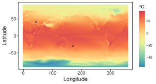
(a) $\{\bar{y}_{A,9}(L_{i},l_{j})\}_{i=1,\ldots,I;j=1,\ldots,J}$

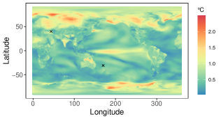
(b) $\{y_{A,9}^{\text{sd}}(L_{i},l_{j})\}_{i=1,\ldots,I;j=1,\ldots,J}$

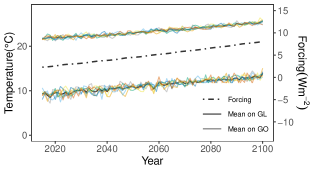
(c) Annual temperature time series

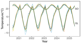
(d) Monthly temperature time series

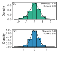
(e) Annual

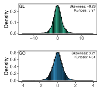
(f) Monthly

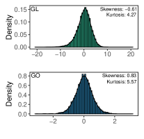
(g) Daily

Figure 1: (a) and (b) are maps of ensemble mean and standard deviation of the annually aggregated temperature at year 2023, where two black “$\times$” represent grid points $(40.05,43.75)$ (GL) and $(-30.63,170.00)$ (GO). (c) shows annual temperature time series at GL and GO, where the solid and dotdash black curves are means over ensembles and the trend of RF, respectively. (d) shows the monthly temperature time series at GL and GO, where the black curves are ensemble means. (e)–(g) are histograms of annual, monthly and daily temperature simulations at GL and GO, which have been detrended by ensemble means. Only data of years 2020, 2040, 2060, 2080, and 2100 are used in daily data.

Let $y_{t}^{(r)}(L_{i},l_{j})$ denote the temperature in Celsius at latitude $L_{i}$, longitude $l_{j}$, time point $t$ after year 2014, and ensemble $r$, where $i=1,\ldots,I$ ($I=192$), $j=1,\ldots,J$ ($J=288$), $t=1,\ldots,T$, and $r=1,\ldots,R$. The value of $T$ varies depending on the temporal resolution chosen, with possible values of $86$, $1032$, or $31,390$. Similarly, let $x_{t}$ represent the RF at time $t$ for all ensembles, as they are generated with the same external forcing. We use members 11 to 17 (out of 20) to illustrate certain data characteristics. Let $y_{A,t}^{(r)}(L_{i},l_{j})$ be the annually aggregated temperature at grid point $(L_{i},l_{j})$, year $t+$2014 and ensemble $r$. Consequently, the ensemble mean and standard deviation at $(L_{i},l_{j})$ and $t+$2014 are denoted as $\bar{y}_{A,t}(L_{i},l_{j})=R^{-1}\sum_{r=1}^{R}y_{A,t}^{(r)}(L_{i},l_{j})$ and $y_{A,t}^{\text{sd}}(L_{i},l_{j})=\{R^{-1}\sum_{r=1}^{R}(y_{A,t}^{(r)}(L_{i},l_{j})-\bar{y}_{A,t}(L_{i},l_{j}))^{2}\}^{1/2}$, respectively. Figs. 1(a) and 1(b) depict maps of $\bar{y}_{A,9}(L_{i},l_{j})$ and $y_{A,9}^{\text{sd}}(L_{i},l_{j})$. Notably, two black “$\times$” marks indicate grid points located at coordinates $(40.05,43.75)$ and $(-30.63,170.00)$, designating points on land (GL) and ocean (GO), respectively. The maps align with the intuitive understanding that temperature generally decreases with increasing latitude.

Let $\{y_{A,t}^{(r)}(L_{i},l_{j})\}_{t=1}^{T}$ represent the annual temperature trajectory of ensemble $r$ at $(L_{i},l_{j})$. Fig. 1(c) illustrates these time series for both GL and GO, i.e., $\{y_{A,t}^{(r)}(\text{GL})\}_{t=1}^{T}$ and $\{y_{A,t}^{(r)}(\text{GO})\}_{t=1}^{T}$, alongside their respective ensemble means $\{\bar{y}_{A,t}(\text{GL})\}_{t=1}^{T}$ and $\{\bar{y}_{A,t}(\text{GO})\}_{t=1}^{T}$. Take $\{y_{A,t}^{(r)}(\text{GL})\}_{t=1}^{T}$ as an example. All ensembles exhibit a shared increasing trend, influenced by the RF also depicted in Fig. 1(c). Moreover, each ensemble exhibits its unique shape, signifying the presence of uncertainty among ensembles. These motivate us to develop an SG incorporating both deterministic and stochastic factors. Similarly, Fig. 1(d) provides monthly temperature time series of years 2021–2025 at GL and GO, along with their respective ensemble means. In comparison to annual data, Fig. 1(d) exhibit a clear seasonality, which is a common feature in monthly and daily data. The time series at GL and GO experience alternating peaks and valleys because they are situated in the northern and southern hemispheres, respectively. Notably, from Figs. 1(c) and 1(d), both the uncertainty and the variation are more pronounced at GL.

Figs. 1(e)–1(g) demonstrate histograms, skewness and kurtosis of the detrended annual, monthly and daily temperature simulations at GL and GO, respectively. For example, the top panel of Fig. 1(e) displays the histogram of $\{y_{A,t}^{(r)}(\text{GL})-R^{-1}\sum_{r=1}^{R}y_{A,t}^{(r)}(\text{GL})\}_{r=1,\ldots,R;t=1,\ldots,T}$ and its skewness and kurtosis. The close-to-zero skewness and the close-to-three kurtosis enable a Gaussian assumption when we model $R$ time series $\{y_{A,t}^{(r)}(\text{GL})-R^{-1}\sum_{r=1}^{R}y_{A,t}^{(r)}(\text{GL})\}_{t=1}^{T}$, with an auto-regression. Fig. S1 presents the skewness and kurtosis for time series across all global grid points. Further assessment through a Jarque-Bera test (Jarque and Bera, 1987) indicates that only $23.3\%$ of grid points with annually aggregated simulations reject the Gaussianity. In contrast, the histograms in Figs. 1(f) and 1(g) tend to be skewed and heavy-tailed. From Fig. S1, the degree of skewness and the presence of heavy tails become more pronounced with increasing temporal resolution, particularly in the band region below latitude $-60^{\circ}$, termed as Band, and the north pole region. Surface temperature simulations exhibit numerical instabilities. The reason will be discussed in Section 4.3. The Jarque-Bera test reveals that about $95\%$ grid points reject the Gaussianity for simulations with higher temporal resolutions. These observations underscore the necessity for additional transformations and parameters to Gaussianize the monthly and daily simulations, as the first two moments alone are insufficient to characterize data with greater temporal complexity.

3 Stochastic Generator Methodology

In this section, we detail the procedures of constructing an SG and generating emulations for the temperature simulations described in Section 2. Leveraging the SHT, our proposed SG offers efficient and adaptable capabilities for dealing with global climate simulations that exhibit: 1) large-scale patterns, 2) non-stationary spatial dependencies among latitudes and land/ocean regions, and 3) non-Gaussian temporal trajectories.

The data characteristics outlined in Section 2 underscore the deterministic chaotic nature inherent in climate models (Lorenz, 1963; Branstator and Teng, 2010; Castruccio and Genton, 2018), which motivates us to decouple the data into deterministic and stochastic components as follows:

$$y_{t}^{(r)}(L_{i},l_{j})=m_{t}(L_{i},l_{j})+\sigma(L_{i},l_{j})Z_{t}^{(r)}(L_{i},l_{j}).\vspace{-20pt}$$ (1)

Here, $m_{t}$ and $\sigma$ are deterministic functions responsible for the mean trend and standard error, respectively, and are shared across all ensembles. $Z_{t}^{(r)}(L_{i},l_{j})$ is the stochastic component at grid point $(L_{i},l_{j})$, time point $t$, and ensemble $r$. Given the expansive parameter space, simultaneously inferring both the deterministic and stochastic components would be computationally infeasible. Therefore, we adopt a two-stage approach, commonly employed in existing work (Castruccio and Genton, 2018; Jeong et al., 2019; Huang et al., 2023). First, we evaluate $m_{t}(L_{i},l_{j})$ and $\sigma(L_{i},l_{j})$ at each grid, making the independence assumption regarding $\{Z_{t}^{(r)}(L_{i},l_{j})\}_{i=1,\ldots,I;j=1,\ldots,J;t=1,\ldots,T;r=1,\ldots,R}$. Subsequently, we analyze the dependence structure of $Z_{t}^{(r)}(L_{i},l_{j})$ by detrending and rescaling $y_{t}^{(r)}(L_{i},l_{j})$ with the estimate of $m_{t}(L_{i},l_{j})$ and $\sigma(L_{i},l_{j})$, respectively.

3.1 Deterministic component of SG

In the first stage of constructing the SG, we focus on determining the mean trend $m_{t}$. It is crucial that the mean trend is both simple enough to minimize the storage requirements for parameters and informative enough to capture the physical relationships between simulations and essential covariates. Let $y_{t}^{(r)}(L_{i},l_{j})$ represent the annually aggregated temperature data. Previous research (Castruccio et al., 2014; Huang et al., 2023) has shown its dependence on the RF trajectory and adopted an infinite distributed lag model:

$$m_{t}(L_{i},l_{j})=\beta_{0}(L_{i},l_{j})+\beta_{1}(L_{i},l_{j})x_{t}+\beta_{2}(L_{i},l_{j})\{1-\rho(L_{i},l_{j})\}\sum_{s=1}^{\infty}\rho(L_{i},l_{j})^{s-1}x_{t-s},\vspace{-20pt}$$

where $\beta_{0}(L_{i},l_{j})$ is the intercept, $\beta_{1}(L_{i},l_{j})$ and $\beta_{2}(L_{i},l_{j})$ are slopes for the current and past RFs, respectively. Lag weights $\beta_{2}(L_{i},l_{j})\{1-\rho(L_{i},l_{j})\}\rho(L_{i},l_{j})^{s-1}$ decrease the impact of past RFs exponentially by $\rho(L_{i},l_{j})\in[0,1]$. Moreover, if $y_{t}^{(r)}(l_{i},l_{j})$ represents the monthly aggregated temperature data, additional harmonic terms $\{\cos(2\pi tk/12),\sin(2\pi tk/12)\}_{k=1}^{K_{M}}$ should be included to fit the interannual cycle as shown in Fig. 1(d). That is,

$$m_{t}(L_{i},l_{j})= \beta_{0}(L_{i},l_{j})+\beta_{1}(L_{i},l_{j})x_{\lceil t/12\rceil}+\beta_{2}(L_{i},l_{j})\{1-\rho(L_{i},l_{j})\}\sum_{s=1}^{\infty}\rho(L_{i},l_{j})^{s-1}x_{\lceil t/12\rceil-s}$$

$$+\sum_{k=1}^{K_{M}}\left\{a_{k}(L_{i},l_{j})\cos\left(\frac{2\pi tk}{12}\right)+b_{k}(L_{i},l_{j})\sin\left(\frac{2\pi tk}{12}\right)\right\},$$

which would also be applied to the daily aggregated temperature by replacing $K_{M}$ and $t/12$ with $K_{D}$ and $t/365$, respectively. For the deterministic component, $\{\beta_{0}(L_{i},l_{j}),\beta_{1}(L_{i},l_{j}),\beta_{2}(L_{i},l_{j})$, $\rho(L_{i},l_{j}),\sigma(L_{i},l_{j}),a_{1}(L_{i},l_{j}),\ldots,a_{K}(L_{i},l_{j}),b_{1}(L_{i},l_{j}),\ldots,b_{K}(L_{i},l_{j})\}_{i=1,\ldots,I;j=1,\ldots,J}$ are all $(5+2K)IJ$ parameters to be evaluated and stored, where $K$ can take values of $0$, $K_{M}$, and $K_{D}$ to represent the annual, monthly and daily temperature, respectively. With the independence assumption, we can efficiently estimate the parameters of the deterministic component in parallel for each grid point. The detailed inferential process is given in Section S3.1 of the Supplementary Materials.

3.2 Stochastic component of SG

Now, we sequentially model the spatial and temporal dependence of the stochastic component $Z_{t}^{(r)}(L_{i},l_{j})$, which is a general principle for analyzing space-time data (Stein, 2007; Castruccio and Genton, 2018) to bypass the prohibitive computation.

3.2.1 Modeling the spatial dependence

The inference of the spatial dependence should consider several crucial factors: 1) The simulations are large-scale; 2) The simulations encompass the entire globe, making the use of chordal distance inappropriate (Jeong et al., 2017); 3) The simulations exhibit non-stationarity among different latitudes and between land and ocean regions. Given these considerations, we propose using the SHT (Jones, 1963; Stein, 2007, 2008), which involves expanding the stochastic component $Z_{t}^{(r)}(L_{i},l_{j})$ with spherical harmonics:

$$Z_{t}^{(r)}(L_{i},l_{j})=\sum_{q=0}^{Q-1}\sum_{m=-q}^{q}(s_{t}^{(r)})_{q}^{m}H_{q}^{m}(L_{i},l_{j})+\varepsilon_{t}^{(r)}(L_{i},l_{j}).\vspace{-10pt}$$ (2)

In (2), $\{H_{q}^{m}\}_{q=0,1,2,\ldots;m=-q,\ldots,q}$ is a complete set of orthonormal basis functions defined in $\mathcal{L}^{2}(\mathbb{S}^{2})$ and indexed by integer degree $q$ and order $m$, where $\mathcal{L}^{2}(\mathbb{S}^{2})$ is the Hilbert space consisting of squared-integrable functions on the sphere $\mathbb{S}^{2}$. The spherical harmonic $H_{m}^{q}$ is a complex-valued function with a closed form $H_{q}^{m}(L_{i},l_{j})=\sqrt{\frac{2q+1}{4\pi}\frac{(q-m)!}{(q+m)!}}P_{q}^{m}(\cos\theta)\exp(\iota m\psi)$, where $\iota^{2}=-1$, $(\theta,\psi)=(\pi L_{i}/180+\pi/2,\pi l_{j}/180)$ is a reparameterization of $(L_{i},l_{j})$ and $P_{q}^{m}$ is the associated Legendre polynomial of degree $q$ and order $m$, such that $H_{q}^{-m}=(-1)^{m}\overline{H_{q}^{m}}$. Corresponding to the $H_{q}^{m}$, $(s_{t}^{(r)})_{q}^{m}$ is the complex-valued spherical harmonic coefficient satisfying $(s_{t}^{(r)})_{q}^{-m}=(-1)^{m}\overline{(s_{t}^{(r)})_{q}^{m}}$. The norm of $(s_{t}^{(r)})_{q}^{m}$, i.e., $\|(s_{t}^{(r)})_{q}^{m}\|_{2}=\sqrt{\Re^{2}\{(s_{t}^{(r)})_{q}^{m}\}+\Im^{2}\{(s_{t}^{(r)})_{q}^{m}\}}$, indicates the energy gathered at degree $q$ and order $m$. $Q$ is an integer ranging from $0$ to $Q_{\max}$, with $Q_{\max}=\min(I,J/2)$ determined by the spatial resolution of the data. The denser the grid points are, the higher the frequency they capture, and the larger the value of $Q_{\max}$ could be. For CESM2-LENS2, $Q_{\max}=144$. The last term $\varepsilon_{t}^{(r)}(L_{i},l_{j})$ accounts for the remaining information and is assumed to be independent and follow $\mathcal{N}(0,v^{2}(L_{i},l_{j}))$. In a physical sense, (2) translates $\{Z_{t}^{(r)}(L_{i},l_{j})\}_{i=1,\ldots,I;j=1,\ldots,J}$ from the spatial domain to $\{(s_{t}^{(r)})_{q}^{m}\}_{q=0,\ldots,Q-1;l=-q,\ldots,q}$ in the spectral domain. In a statistical sense, with $Q\ll\sqrt{IJ}$, (2) provides a low-rank approximation for the stochastic process $Z_{t}$, where $(s_{t})_{q}^{m}$ serves as a random coefficient and $Q$ trades off the quality of approximation against the computational complexity.

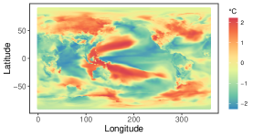
(a) Spatial domain

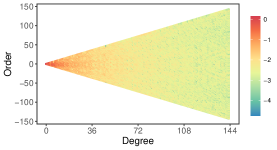
(b) Spectral domain

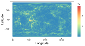
(c) $Q=36$

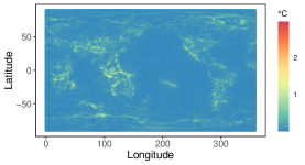
(d) $Q=72$

Figure 2: (a) shows a set of stochastic component $\{Z_{9}^{(1)}(L_{i},l_{j})\}_{i=1,\ldots,I;j=1,\ldots,J}$ in spatial domain. (b) indicates energy allocation of (a) in spectral domain. (c) and (d) show the loss of performing SHT or the low-rank approximation with different $Q$ values.

We provide Fig. 2 to facilitate the understanding of SHT. Fig. 2(a) shows a set of stochastic components in the spatial domain, i.e., $\{Z_{9}^{(1)}(L_{i},l_{j})\}_{i=1,\ldots,I;j=1,\ldots,J}$, which is obtained by detrending and rescaling the annually aggregated temperature at year 2023 and ensemble one with ensemble mean and standard error in Figs. 1(a) and 1(b), respectively. After applying the SHT, Fig. 2(b) presents the pattern of $\{\log_{10}\|(s_{9}^{(1)})_{q}^{m}\|_{2}\}_{q=0,1,\ldots,Q_{max};m=-q,\ldots,q}$, which indicates the energy allocation in the spectral domain. The energy is more concentrated at lower degrees of lower frequencies, gradually decreasing as the degree increases. Figs. 2(c) and 2(d) depict the absolute values of $\{\varepsilon_{9}^{(1)}(L_{i},l_{j})\}_{i=1,\ldots,I;j=1,\ldots,J}$ with $Q=36$ and $72$, respectively, which highlight the influence of $Q$ on the loss of SHT or the accuracy of approximation. A larger value of $Q$ retains more information and provides a better approximation. Moreover, the temperature variability over land and ocean may occur at different scales. More spherical harmonics, or say, more basis functions with higher resolution, are needed to capture the high-frequency variation on ocean.

We emphasize the advantages of employing the SHT as a low-rank approximation to handle large-scale climate simulations: 1) Natual basis functions. Unlike existing methods (Nychka et al., 2015; Katzfuss, 2017; Tzeng and Huang, 2018) that use basis functions mathematically developed without a clear physical meaning, the SHT utilizes spherical harmonics, which are the eigen-functions of the Laplace-Beltrami operator. This makes the SHT particularly suitable for analyzing spherical data, such as global climate simulations. The SHT transforms data from the spatial domain to the spectral domain, providing a different perspective for data analysis. This spectral view can reveal hidden patterns and characteristics of the data that may not be as apparent in the spatial domain; 2) Automatic multiresolution. Spherical harmonics are naturally organized in order of their degrees. This inherent multiresolution property allows them to capture information at various scales without the need for manually allocating knots or tuning parameters. Researchers need only select the maximum degree $Q$, to control the level of detail; 3) Efficient computational implementation. Both the SHT and its inverse can be efficiently calculated with a computational time that scales as $O(Q^{3})$ for a given degree $Q$. Moreover, this computational time can be further reduced to $O(Q^{2})$ by parallel computing. On a MacBook with a $3.2$ GHz Apple M1 Pro processor with ten cores, performing the SHT with $Q=Q_{\max}$ in Fig. 2 takes about $3$ seconds, and the inverse SHT with $Q=36$, $72$, and $144$ take no more than $0.06$, $0.3$, and $2$ seconds, respectively.

Next, we model the spatial dependence structure, which is assumed to remain consistent over time. The covariance between $Z_{t}(L_{i},l_{j})$ and $Z_{t}(L_{i^{\prime}},l_{j^{\prime}})$ is

$$c\{(L_{i},l_{j}),(L_{i^{\prime}},l_{j^{\prime}})\}=\mathrm{Cov}\{Z_{t}(L_{i},l_{j}),Z_{t}(L_{i^{\prime}},l_{j^{\prime}})\}=\mathbf{H}(L_{i},l_{j})^{\top}\mathbf{K}\overline{\mathbf{H}(L_{i},l_{j})}+\delta_{i=i^{\prime}}\delta_{j=j^{\prime}}v^{2}(L_{i},l_{j}),\vspace{-20pt}$$ (3)

where $\mathbf{K}=\mathbf{K}_{t}=\mathrm{E}(\mathbf{s}_{t}\mathbf{s}_{t}^{\mathrm{H}})$ is a $Q^{2}\times Q^{2}$ covariance matrix of $\{(s_{t})_{q}^{m}\}_{q=0,1,\ldots,Q;m=-q,\ldots,q}$, $\mathrm{H}$ is the operator of conjugate transpose, $\mathbf{H}(L_{i},l_{j})$ and $\mathbf{s}_{t}$ are vectors consisting of basis functions and spherical harmonic coefficients, indexed by $(q^{2}+q+m+1)$. Specifically, the $(q^{2}+q+m+1)$th elements of $\mathbf{H}(L_{i},l_{j})$ and $\mathbf{s}_{t}$ are $H_{q}^{m}(L_{i},l_{j})$ and $(s_{t})_{q}^{m}$, respectively.

Further examining the structure of $\mathbf{K}$, it is evident that the stochastic component in Fig. 2(a) exhibits strong heterogeneity across different latitudes, as observed in previous studies of global climate data (Stein, 2007; Jeong et al., 2018; Huang et al., 2023). Consequently, the commonly used isotropic assumption for Euclidean data is no longer appropriate. Instead, we adopt the assumption of axial symmetry, which posits that only data on the same latitude are stationary (Jones, 1963). This leads to the covariance $c\{(L_{i},l_{j}),(L_{i^{\prime}},l_{j^{\prime}})\}$ becoming a function of $L_{i}$ ($\theta$), $L_{i^{\prime}}$ ($\theta^{\prime}$), and $|l_{j}-l_{j^{\prime}}|$ ($|\psi-\psi^{\prime}|$, the central angle between points $(L_{i},l_{j})$ and $(L_{i^{\prime}},l_{j^{\prime}})$ expressed in chordal distance). Using a simple derivation outlined in Jones (1963), we have

$$c(L_{i},L_{i^{\prime}},|l_{j}-l_{j^{\prime}}|)=\sum_{q=0}^{Q-1}\sum_{q^{\prime}=0}^{Q-1}\sum_{m=-q}^{q}k_{qq^{\prime}m}H_{q}^{m}(\theta,0)H_{q^{\prime}}^{m}(\theta^{\prime},0)\exp(\iota m|\psi-\psi^{\prime}|)\vspace{-10pt}$$ (4)

with $\mathrm{E}\{(s_{t})_{q}^{m}(s_{t})_{q^{\prime}}^{m^{\prime}}\}=\delta_{m=m^{\prime}}k_{qq^{\prime}m}$. It means that axial symmetry assumes dependence only on coefficients of the same order. Thus, $\mathbf{K}$ becomes a sparse matrix, consisting of $Q^{2}+(Q-1)^{2}+\cdots+1^{2}=Q^{3}/3+Q^{2}/2+Q/6$ non-zero elements.

However, from Figs. 1 and 2, we still observe heterogeneity between land and ocean data on the same latitude. Land and ocean temperatures exhibit variations on different scales, requiring different numbers of basis functions to capture adequately. Therefore, we propose replacing (2) by

$$Z_{t}^{(r)}(L_{i},l_{j})=\sum_{q=0}^{Q_{l}-1}\sum_{m=-q}^{q}(s_{t}^{(r)})_{q}^{m}H_{q}^{m}(L_{i},l_{j})+\delta_{(L_{i},l_{j})\in\mathcal{S}_{o}}\sum_{q=Q_{l}}^{Q_{o}-1}\sum_{m=-q}^{q}(s_{t}^{(r)})_{q}^{m}H_{q}^{m}(L_{i},l_{j})+\varepsilon_{t}^{(r)}(L_{i},l_{j}),\vspace{-10pt}$$ (5)

where $S_{o}$ represents the set of grid points over the ocean, $Q_{l}$ and $Q_{o}>Q_{l}$ denote the values of $Q$ for land and ocean, respectively. We ignore the continuity of temperature changes between land and ocean, since (5) is formulated on grid points and our target is not to predict at new points. Accordingly, the covariance $c_{t}(L_{i},L_{i},|l_{j}-l_{j^{\prime}}|)$ is given by plugging the $Q$ values of $(L_{i},l_{j})$ and $(L_{i^{\prime}},l_{j^{\prime}})$ into (4). We present the process of choosing appropriate values for $Q_{o}$ and $Q_{l}$ in Section 4.

3.2.2 Modeling the temporal dependence

Next, we investigate the temporal dependence within the vector time series $\{\mathbf{s}_{t}^{(r)}\}_{t=1}^{T}$ in the spectral domain. We will employ an auto-regressive model, but with two additional operations: converting the coefficients to real-valued ones and Gaussianizing them using the TGH transformation. Specifically, for the complex-valued vector $\mathbf{s}_{t}^{(r)}$ with the special structure of $(s_{t}^{(r)})_{q}^{-m}=(-1)^{m}\overline{(s_{t}^{(r)})_{q}^{m}}$, we first linearly transform it into a real-valued vector

$$\tilde{\mathbf{s}}_{t}^{(r)}=\mathbf{A}^{-1}\mathbf{s}_{t}^{(r)}=[(s_{t}^{(r)})_{0}^{0},\Im\{(s_{t}^{(r)})_{1}^{1}\},(s_{t}^{(r)})_{1}^{0},\Re\{(s_{t}^{(r)})_{1}^{1}\},\ldots,\Im\{(s_{t}^{(r)})_{Q-1}^{Q-1}\},\ldots,\Re\{(s_{t}^{(r)})_{Q-1}^{Q-1}\}]^{\top},\vspace{-20pt}$$

where both $\mathbf{A}$ and its inverse are $Q^{2}\times Q^{2}$ sparse matrices with known structures. For example, in the case of $Q=2$, $\mathbf{A}$ and $\mathbf{A}^{-1}$ can be represented as

$$\left(\begin{array}[]{cccc}1&0&0&0\\[-10.76385pt] 0&\iota&0&-1\\[-10.76385pt] 0&0&1&0\\[-10.76385pt] 0&\iota&0&1\end{array}\right)\quad\text{and}\quad\left(\begin{array}[]{cccc}1&0&0&0\\[-10.76385pt] 0&-\iota/2&0&-\iota/2\\[-10.76385pt] 0&0&1&0\\[-10.76385pt] 0&-1/2&0&1/2\end{array}\right),\vspace{-10pt}$$

respectively. For simplicity, we denote the $(q^{2}+q+m+1)$th element of $\tilde{\mathbf{s}}_{t}^{(r)}$ as $(\tilde{s}_{t}^{(r)})_{q}^{m}$. Consequently, we have $Z_{t}^{(r)}(L_{i},l_{j})=\mathbf{H}(L_{i},l_{j})^{\top}\mathbf{A}\tilde{\mathbf{s}}_{t}^{(r)}+\varepsilon_{t}^{(r)}(L_{i},l_{j})$, where $\mathbf{A}^{\top}\mathbf{H}(L_{i},l_{j})$ and $\tilde{\mathbf{s}}_{t}^{(r)}$ are vectors of bases and coefficients, respectively. Under the assumption of axial symmetry, the covariance matrix of $\tilde{\mathbf{s}}$, denoted as $\tilde{\mathbf{K}}=\mathrm{E}(\tilde{\mathbf{s}}\tilde{\mathbf{s}}^{\top})$, is also a sparse matrix. Specifically, $\mathrm{E}(\tilde{s}_{q}^{m}\tilde{s}_{q^{\prime}}^{m^{\prime}})=\mathrm{E}(\tilde{s}_{q}^{-m}\tilde{s}_{q^{\prime}}^{-m^{\prime}})=\tilde{k}_{qq^{\prime}m}\delta_{m=m^{\prime}}\delta_{m\geq 0}$. The derivation is given in Section S3.2 of Supplementary Materials. The matrix $\tilde{\mathbf{K}}$ consists of $2Q^{3}/3+Q/3$ non-zero elements and only $Q^{3}/3+Q^{2}/2+Q/3$ ones need to be stored.

If $Z_{t}^{(r)}(L_{i},l_{j})$ represents the stochastic component of annually aggregated temperature, it is reasonable to assume the Gaussianity of $\{Z_{t}^{(r)}(L_{i},l_{j})\}_{t=1}^{T}$, and therefore, the Gaussianity of $\{\tilde{\mathbf{s}}_{t}^{(r)}\}_{t=1}^{T}$. This allows us to model it with a vector auto-regressive model of order $P$ (VAR($P$)): $\tilde{\mathbf{s}}_{t}^{(r)}=\sum_{p=1}^{P}\bm{\Phi}_{p}\tilde{\mathbf{s}}_{t-p}^{(r)}+\bm{\xi}_{t}^{(r)}$, where $\bm{\xi}_{t}^{(r)}\overset{i.i.d.}{\sim}\mathcal{N}_{Q^{2}}(\mathbf{0},\mathbf{U})$ and $\mathbf{U}=\tilde{\mathbf{K}}-\sum_{p=1}^{P}\bm{\Phi}_{p}\tilde{\mathbf{K}}\bm{\Phi}_{p}^{\top}$.

However, as in Section 2, when $Z_{t}^{(r)}(L_{i},l_{j})$ is the stochastic component of the monthly or daily aggregated temperature, the Gaussianity assumption for time series $\{Z_{t}^{(r)}(L_{i},l_{j})\}_{t=1}^{T}$ at most grid points $(L_{i},l_{j})$ may not hold. It implies that $\{(\tilde{s}_{t}^{(r)})_{q}^{m}\}_{t=1}^{T}$ at some $(q,m)$ pairs are not Gaussian and motivates us to employ a modified TGH transformation. Denote by $\mathcal{S}_{gh}$ the set of $(q,m)$ such that $\{(\tilde{s}_{t}^{(r)})_{q}^{m}\}_{t=1}^{T}$ rejects the Gaussianity. We model the coefficients with a TGH auto-regressive model: $\check{\mathbf{s}}_{t}^{(r)}=\sum_{p=1}^{P}\bm{\Phi}_{p}\check{\mathbf{s}}_{t-p}^{(r)}+\bm{\xi}_{t}^{(r)}$, where the $(q^{2}+q+m+1)$th element of $\check{\mathbf{s}}_{t}^{(r)}$ is

$$(\check{s}_{t}^{(r)})_{q}^{m}=\left\{\begin{array}[]{lr}\lambda_{q}^{m}\tau_{g_{q}^{m},h_{q}^{m}}^{-1}\{(\tilde{s}_{t}^{(r)})_{q}^{m}/\omega_{q}^{m}\},&\text{if}\quad(q,m)\in\mathcal{S}_{gh},\\ (\tilde{s}_{t}^{(r)})_{q}^{m},&\text{if}\quad(q,m)\notin\mathcal{S}_{gh},\end{array}\right.\vspace{-10pt}$$ (6)

with $\tau_{g_{q}^{m},h_{q}^{m}}(s)=(g_{q}^{m})^{-1}\{\exp(g_{q}^{m}s)-1\}\exp(h_{q}^{m}s^{2}/2)$. Compared to the regular TGH, the one in (6) removes a location parameter and introduces a scale parameter $\lambda_{q}^{m}$. The former is due to the zero-mean $\{(\tilde{s}_{t}^{(r)})_{q}^{m}\}_{t=1,\ldots,T;r=1,\ldots,R}$. The later ensures the standard deviation of $\{(\check{s}_{t}^{(r)})_{q}^{m}\}_{t=1,\ldots,T;r=1,\ldots,R}$ to be equal to that of $\{(\tilde{s}_{t}^{(r)})_{q}^{m}\}_{t=1,\ldots,T;r=1,\ldots,R}$. Four additional parameters describing characteristics beyond the first two moments are to be stored. Based on (6), the covariance matrix of $\bm{\xi}_{t}^{(r)}$ is $\mathbf{U}=\check{\mathbf{K}}-\sum_{p=1}^{P}\bm{\Phi}_{p}\check{\mathbf{K}}\bm{\Phi}_{p}^{\top}$, where $\check{\mathbf{K}}=\mathrm{E}(\check{\mathbf{s}}\check{\mathbf{s}}^{\top})$ also has the sparse structure $\mathrm{E}(\check{s}_{q}^{m}\check{s}_{q^{\prime}}^{m^{\prime}})=\mathrm{E}(\check{s}_{q}^{-m}\check{s}_{q^{\prime}}^{-m^{\prime}})=\check{k}_{qq^{\prime}m}\delta_{m=m^{\prime}}\delta_{m\geq 0}$ under the assumption of axial symmetry.

Furthermore, we assume that $\bm{\Phi}_{p}$ is a diagonal matrix with the $(q^{2}+q+m+1)$th diagonal element denoted as $(\phi_{p})_{q}^{m}$. This assumption neglects the cross dependence between $\{(\tilde{s}_{t}^{(r)})_{q}^{m}\}_{q=0,\ldots,Q-1;m=-q,\ldots,q}$, and hence enables the independent and parallel evaluation of $\{(\phi_{p})_{q}^{m}\}_{p=1}^{P}$ across $q$ and $m$. We briefly validated it in Section S3.3 by testing the significance of the first temporal lag of the cross-correlation. The proportion of $p$-values less than 0.05 is nearly zero, indicating the negligible cross-dependence. The details about the parameter estimation are given in Section S3.4.

3.3 Emulation with SG

The procedures of constructing an SG for the monthly and daily temperature simulations from CESM2-LENS2 is summarized in Algorithm S1. We assume that the tuning parameters $K$, $Q_{l}$, $Q_{o}$, and $P$ are known. More details about their selection will be provided in Section 4. In Stage 1, we calculate and store a total of $(5+2K)IJ$ parameters in the deterministic component. In Step 1) of Stage 2, although we use different $Q$ values for land and ocean data to evaluate $v(L_{i},l_{j})$, we still need coefficients up to degree $Q_{o}$. The number of stored parameters in Stage 2 is $IJ+(4+P)Q_{o}^{2}+(Q_{o}^{3}/3+Q_{o}^{2}/2+Q_{o}/3)$. Therefore, the total number of parameters is of the order $O(IJ+Q_{o}^{3})$. For the annually aggregated temperature, there is no need to perform a TGH transformation in Step 3) of Stage 2. Consequently, $\mathcal{S}_{gh}$ is an empty set, and only $IJ+PQ_{o}^{2}+(Q_{o}^{3}/3+Q_{o}^{2}/2+Q_{o}/3)$ parameters are needed for the stochastic component. In summary, we develop an SG by training on simulations of size $IJRT$ and store it for generating unlimited emulations using at most $(6+2K)IJ+(4+P)Q_{o}^{2}+(Q_{o}^{3}/3+Q_{o}^{2}/2+Q_{o}/6)$ memorized parameters.

We compare our SG with that of Huang et al. (2023) proposed for LENS1 (Kay et al., 2015). Their method was primarily developed within the spatial domain and required memorization of $(2K+P+8)IJ+6I$ parameters. This consisted of $(5+2K)IJ$ parameters for the deterministic component, $PIJ$ parameters for evaluating the temporal dependence, $3IJ$ parameters for TGH transformation, and $6I$ parameters for assessing the non-stationary spatial dependence. With $P=1$ and $Q_{o}=70$, which maximizes storage requirements for our method, Huang et al. (2023) necessitate an additional $25,745$ parameters. Hence, our SG offers a significant advantage in terms of parameter storage efficiency.

In Algorithm 1, we outline the procedures for generating monthly and daily temperature emulations for CESM2-LENS2. Note that a Cholesky decomposition should be performed on $\mathbf{U}$ when generating $\check{\mathbf{s}}_{t}^{(r^{\prime})}$, which may be time-consuming if $Q_{o}$ is not small. However, the sparse structure of $\mathbf{U}$ avoids the possible computational limitation. For the annually aggregated temperature, we can simply remove Step (b) in Stage 2 and replace $\tilde{\mathbf{s}}_{SG,t}^{(r^{\prime})}$ in Step (c) with $\check{\mathbf{s}}_{SG,t}^{(r^{\prime})}$.

Algorithm 1 Emulation with SG

0:  $\rho(L_{i},l_{j})$, $\beta_{0}(L_{i},l_{j})$, $\beta_{1}(L_{i},l_{j})$, $\beta_{2}(L_{i},l_{j})$, $a_{1}(L_{i},l_{j})$,…, $a_{K}(L_{i},l_{j})$, $b_{1}(L_{i},l_{j})$,…, $b_{K}(L_{i},l_{j})$, $\sigma(L_{i},l_{j})$, $v(L_{i},l_{j})$, $\lambda_{q}^{m}$, $\omega_{q}^{m}$, $g_{q}^{m}$, $h_{q}^{m}$, $(\phi_{1})_{q}^{m},\ldots,(\phi_{P})_{q}^{m}$, $i=1,\ldots,I$, $j=1,\ldots,J$, $q=0,\ldots,Q_{o}-1$, $m=-q,\ldots,q$, $\check{\mathbf{K}}$, $Q_{l}$, $Q_{o}$, $K$, $P$, $\mathbf{A}\in\mathbb{R}^{Q_{o}^{2}\times Q_{o}^{2}}$, $R^{\prime}$.

0:   1) For each grid point $(L_{i},l_{j})$, calculate $\{m_{t}(L_{i},l_{j})\}_{t=1}^{T}$ and $\sigma(L_{i},l_{j})$ with given parameters of the deterministic component, $i=1,\ldots,I$ and $j=1,\ldots,J$. 2) Calculate $\mathbf{U}=\check{\mathbf{K}}-\sum_{p=1}^{P}\Phi_{p}\check{\mathbf{K}}\Phi_{p}^{\top}$.

0:   For $r^{\prime}=1,\ldots,R^{\prime}$: 1) generate $\check{\mathbf{s}}_{SG,-(p-1)}^{(r^{\prime})}\sim\mathcal{N}_{Q_{o}^{2}}(\mathbf{0},\mathbf{U})$, $p=1,\ldots,P$, 2) for $t=1,\ldots,T$:       (a) generate $\bm{\xi}_{SG,t}^{(r^{\prime})}\sim\mathcal{N}_{Q_{o}^{2}}(\mathbf{0},\mathbf{U})$, and calculate $\check{\mathbf{s}}_{SG,t}^{(r^{\prime})}=\sum_{p=1}^{P}\Phi_{p}\check{\mathbf{s}}_{SG,t-p}^{(r^{\prime})}+\bm{\xi}_{SG,t}^{(r^{\prime})}$,       (b) calculate $\tilde{\mathbf{s}}_{SG,t}^{(r^{\prime})}$, where $(\tilde{s}_{SG,t}^{(r^{\prime})})_{q}^{m}=\omega_{q}^{m}\tau_{g_{q}^{m},h_{q}^{m}}\{(\check{s}_{SG,t}^{(r^{\prime})})_{q}^{m}/\lambda_{q}^{m}\}$,       (c) calculate $\mathbf{s}_{SG,t}^{(r^{\prime})}=\mathbf{A}\tilde{\mathbf{s}}_{SG,t}^{(r^{\prime})}$, and perform the inverse SHT on $\mathbf{s}_{SG,t}^{(r^{\prime})}$ with (5) to obtain $\{\mathrm{invSHT}(\mathbf{s}_{SG,t}^{(r^{\prime})})(L_{i},l_{j})\}_{i=1,\ldots,I;j=1,\ldots,J}$,       (d) generate $\varepsilon_{SG,t}^{(r^{\prime})}(L_{i},l_{j})\sim\mathcal{N}(0,\hat{v}(L_{i},l_{j})^{2})$, $i=1,\ldots,I;j=1,\ldots,J$;       (e) generate emulations

$$y_{SG,t}^{(r^{\prime})}(L_{i},l_{j})=m_{t}(L_{i},l_{j})+\sigma(L_{i},l_{j})\{\mathrm{invSHT}(\mathbf{s}_{SG,t}^{(r^{\prime})})(L_{i},l_{j})+\varepsilon_{SG,t}^{(r^{\prime})}(L_{i},l_{j})\}.\vspace{-5pt}$$

0:  $\{y_{SG,t}^{(r^{\prime})}(L_{i},l_{j})\}_{i=1,\ldots,I;j=1,\ldots,J;r^{\prime}=1,\ldots,R^{\prime}}$.

4 Case Study: CESM2-LENS2

In this section, we develop emulators and generate emulations for the annual, monthly and daily aggregated temperature data from CESM2-LENS2 using the proposed algorithms. We provide more details about the implementation, including the choice of tuning parameters and the modeling of the dependence structure. Additionally, we assess the performance of our SGs, which relies on the specific purpose for which the emulator is intended (Castruccio et al., 2014).

Our main goal is to generate emulations that closely resemble the given simulations. To achieve this, our SG should efficiently decouple and capture the deterministic and stochastic components of the data. First, $m_{t}$ should mimic and extract the variation of the ensemble mean in the simulations. After adding the stochastic component, the variability of emulations should be similar to the internal variability observed in simulations. To assess the performance of our SGs, we will discuss two key factors: goodness-of-fit and variability, which are quantified with numerical indices. Moreover, we will conduct visual and numerical comparisons of various characteristics between the simulations. This ensures that our emulations faithfully capture the essential features of the temperature data from CESM2-LENS2.

4.1 Annually aggregated temperature

When working with annually aggregated temperature simulations $\{y_{t}^{(r)}(L_{i},l_{j})\}_{i=1,\ldots,I;j=1,\ldots,J;t=1,\ldots,T;r=1,\ldots,R}$, with a total of $T=86$ time points, we need to evaluate the deterministic component $m_{t}$ and $\sigma$ first, which we denoted as $\hat{m}_{t}$ and $\hat{\sigma}$. Ideally, we hope that $\hat{m}_{t}$ with $4IJ$ parameters could perform comparably to the ensemble mean $\bar{y}_{t}=R^{-1}\sum_{r=1}^{R}y_{t}^{(r)}$ with $TIJ$ parameters. As in Castruccio et al. (2014, 2019), we use

$$\mathrm{I}_{\rm fit}(L_{i},l_{j})=\frac{\sum_{r=1}^{R}\sum_{t=1}^{T}\{y_{t}^{(r)}(L_{i},l_{j})-\hat{m}_{t}(L_{i},l_{j})\}^{2}}{R/(R-1)\sum_{r=1}^{R}\sum_{t=1}^{T}\{y_{t}^{(r)}(L_{i},l_{j})-\bar{y}_{t}(L_{i},l_{j})\}^{2}}\vspace{-10pt}$$

to assess the goodness-of-fit of the SG. The closer the $\mathrm{I}_{\rm fit}$ value to $1$, the better the ability of the SG to capture the variability of the ensemble mean.

Fig. 3(a) presents boxplots of $\{\mathrm{I}_{\rm fit}(L_{i},l_{j})\}_{i=1,\ldots,I;j=1,\ldots,J}$ for different values of $R$. These values tend to get closer to $1$ as $R$ increases, and they stabilize after $R\geq 7$, which means that using seven training simulations is sufficient to stabilize the inference. Therefore, we select $R=7$ for the subsequent analysis. The corresponding $\{\mathrm{I}_{\rm fit}(L_{i},l_{j})\}_{i=1,\ldots,I;j=1,\ldots,J}$ values are shown in Fig. 5(a), with a median value of $1.001$. Temperature can be fitted well at most grid points. Furthermore, Fig. 3(b) displays the map of $\hat{\sigma}(L_{i},l_{j})$, illustrating the non-stationarity of the data. It is evident that larger-scale variation is observed over land.

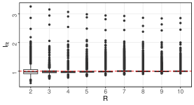
(a) $\mathrm{I}_{\rm fit}$ versus $R$

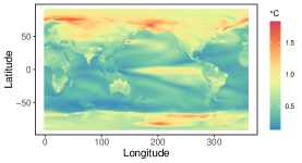
(b) $\hat{\sigma}(L_{i},l_{j})$

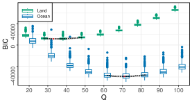
(c) Choice of $Q$

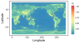
(d) $\hat{v}(L_{i},l_{j})$

Figure 3: (a) shows boxplots of $\{\mathrm{I}_{\rm fit}(L_{i},l_{j})\}_{i=1,\ldots,I;j=1,\ldots,J}$ for different values of $R$. (b) is the map of the estimated standard deviation $\{\hat{\sigma}(L_{i},l_{j})\}_{i=1,\ldots,I;j=1,\ldots,J}$. (c) shows boxplots of $\{\mathrm{BIC}_{*,t}^{(r)}(Q)\}_{r=1,\ldots,R;t=1,\ldots,T}$ for different values of $Q$, where $*$ takes “l” and “o”. Points $\times$ show medians of BIC values. The red points indicate the minimum values. (d) is the map of $\{\hat{v}(L_{i},l_{j})\}_{i=1,\ldots,I;j=1,\ldots,J}$.

Then, we perform the SHT on the stochastic component, necessitating the selection of appropriate values for $Q_{l}$ and $Q_{o}$. Based on the Gaussian assumption of $\varepsilon_{t}^{(r)}(L_{i},l_{j})$, we propose a Bayesian information criterion (BIC) for $\{Z_{t}^{(r)}(L_{i},l_{j})\}_{i=1,\ldots,I;j=1,\ldots,J}$ at time $t$ of ensemble $r$:

$$\mathrm{BIC}_{*,t}^{(r)}(Q)=\log(n_{*})Q^{2}+n_{*}\log(2\pi)+\delta_{(L_{i},l_{j})\in\mathcal{S}_{*}}\sum_{i=1}^{I}\sum_{j=1}^{J}\log\{\hat{v}^{2}(L_{i},l_{j})\}+\delta_{(L_{i},l_{j})\in\mathcal{S}_{*}}\sum_{i=1}^{I}\sum_{j=1}^{J}\left\{\frac{\varepsilon_{t}^{(r)}(L_{i},l_{j})}{\hat{v}(L_{i},l_{j})}\right\}^{2},\vspace{-10pt}$$

where $\hat{v}^{2}(L_{i},l_{j})=(RT)^{-1}\sum_{r=1}^{R}\sum_{t=1}^{T}\{\varepsilon_{t}^{(r)}(L_{i},l_{j})\}^{2}$. When $*$ takes “o”, the above BIC with $n_{o}=\sum_{i=1}^{I}\sum_{j=1}^{J}\delta_{(L_{i},l_{j})}\in\mathcal{S}_{o}$ helps select an appropriate $Q_{o}$ for $Z_{t}^{(r)}(L_{i},l_{j})$ over the ocean, with $\mathcal{S}_{o}$ representing the set of grid points over ocean. Similarly, when $*$ is “l”, it leads to the determination of $Q_{l}$. Fig. 3(c) illustrates boxplots of $\{\mathrm{BIC}_{*,t}^{(r)}\}_{r=1,\ldots,R;t=1,\ldots,T}$ against different values of $Q$, revealing a substantial discrepancy in preferred $Q$ values between land and ocean. The stochastic component on land exhibits large-scale variations, favoring smaller $Q_{l}$ values and treating additional harmonic terms as “noise”. Consequently, its residual information $\varepsilon_{t}^{(r)}(L_{i},l_{j})$ also displays larger-scale variations, as depicted in the rough sketch of land in Fig. 3(d). In contrast, the stochastic components over the ocean vary on a smaller scale, need more harmonics of high frequency, and hence prefer larger $Q_{o}$. The $\times$ points in Fig. 3(c) provide further insight into the trends of BIC, leading us to select $Q_{l}=35$ and $Q_{o}=69$ to minimize the medians of BIC for land and ocean, respectively.

Next, we assess the temporal dependence by fitting $\{(\tilde{s}_{t}^{(r)})_{q}^{m}\}_{t=1,\ldots,T;r=1,\ldots,R}$ with the VAR($P$) model. For each $(q,m)$, we suggest to choose $P$ by minimizing $\mathrm{BIC}_{q}^{m}(P)=P\log\{(T-P)R\}+R(T-P)\log(2\pi)+R(T-P)\log((\hat{u}_{q}^{m})^{2})$, where $(\hat{u}_{q}^{m})^{2}=R^{-1}(T-P)^{-1}\sum_{r=1}^{R}\sum_{t=P+1}^{T}\{(\tilde{s}_{t}^{(r)})_{q}^{m}-\sum_{p=1}^{P}(\phi_{p})_{q}^{m}(\tilde{s}_{t-p}^{(r)})_{q}^{m}\}^{2}$. For briefness, we use the conditional log-likelihood (given $(\tilde{s}_{1}^{(r)})_{q}^{m},\ldots,(\tilde{s}_{P}^{(r)})_{q}^{m}$) rather than an exact log-likelihood in the above BIC. The proportions of $P=1,\ldots,5$ are $99.3\%$, $0.2\%$, $0.2\%$, $0.1\%$, and $0.2\%$, respectively. Therefore, we opt for $P=1$ for the annual case. Fig. 4(a) further demonstrates the estimates of $\{(\phi_{1})_{q}^{m}\}_{q=0,\ldots,Q_{o}-1;m=-q,\ldots,q}$.

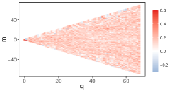
(a) $(\hat{\phi}_{1})_{q}^{m}$

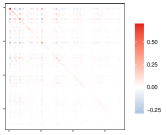
(b) $\tilde{\mathbf{K}}_{\mathrm{emp}}$

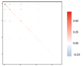
(c) $\tilde{\mathbf{K}}_{\mathrm{axl}}$

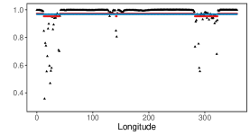
(d) Auto-covariance at $L_{i}=-11.8^{\circ}$

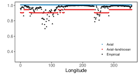
(e) Auto-covariance at $L_{i}=36.3^{\circ}$

Figure 4: Temporal and spatial dependence structure. (a) is the map of the estimated $\{(\phi_{1})_{q}^{m}\}_{q=0,\ldots,Q_{o}-1;m=-q,\ldots,q}$ for the annual simulations. (b) is the first $69$ rows and columns of $\tilde{\mathbf{K}}$ empirically evaluated by $(RT)^{-1}\sum_{r=1}^{R}\sum_{t=1}^{T}\tilde{\mathbf{s}}_{t}^{(r)}\tilde{\mathbf{s}}_{t}^{(r)\top}$ and denoted as $\tilde{\mathbf{K}}_{\mathrm{emp}}$. (c) is the first $69$ rows and columns of $\tilde{\mathbf{K}}$ evaluated under the axial symmetric assumption and denoted as $\tilde{\mathbf{K}}_{\mathrm{axl}}$. (d) and (e) show empirical and fitted auto-covariance at latitudes $-11.8^{\circ}$ and $36.3^{\circ}$, respectively.

Finally, we evaluate the spatial dependence by examining the matrix $\tilde{\mathbf{K}}$. Figs. 4(b) and 4(c) show top-left corners of two evaluations of $\tilde{\mathbf{K}}$. $\tilde{\mathbf{K}}_{\mathrm{emp}}$ is the sample covariance matrix of $\tilde{\mathbf{s}}_{t}^{(r)}$, forming a dense $Q_{o}^{2}\times Q_{o}^{2}$ matrix and serving as a comparison for $\tilde{\mathbf{K}}_{\mathrm{axl}}$. In Algorithm S1, we calculate $\tilde{\mathbf{K}}_{\rm axl}$, which is a sparse matrix, facilitating storage and efficient operations. In Algorithm 1, $\tilde{\mathbf{U}}$ inherits the sparsity characteristics of $\tilde{\mathbf{K}}_{\rm axl}$, enabling fast Cholesky decomposition using efficient algorithms (Furrer and Sain, 2010). Figs. 4(d) and 4(e) display empirical and fitted covariances for $Z(L_{i},l_{j})$ and $Z(L_{i},l_{j+1})$, specifically the auto-covariance $\{\mathrm{cov}\{Z(L_{i},l_{j}),Z(L_{i},l_{j+1})\}\}_{j=1}^{J-1}$ at $L_{i}=-11.8^{\circ}$ and $36.3^{\circ}$. These plots highlight the distinction between the proposed separate SHT for land and ocean (5) (Axial-land/ocean) and the original SHT (2) (Axial). The empirical auto-covariance over ocean appears almost flat, supporting the assumption of axial symmetry over the ocean. In contrast, the auto-covariance over land significantly differs from that over the ocean. This difference is not captured by the fitted covariance of Axial, which selects $Q=77$ via BIC. Axial-land/ocean fits the covariance separately for land and ocean, resulting in segmented lines in Figs. 4(d) and 4(e). However, land temperature exhibits a complex and non-stationary dependence structure, with covariance weakening as one moves farther inland. This intricacy warrants further investigation in future research.

Inputting the above-estimated parameters, we generate $R^{\prime}=R=7$ emulations with Algorithm 1. Each emulation takes approximately $30$ seconds to produce without parallel computation. To assess the variability of these emulations, we employ $\mathrm{I}_{\rm uq}$, a measure proposed in Huang et al. (2023), which leverages the concept of functional data depths (López-Pintado and Romo, 2009). In particular, we treat $\{y_{SG,t}^{(r^{\prime})}(L_{i},l_{j})\}_{r^{\prime}=1}^{R^{\prime}}$ as $R^{\prime}$ functions of $t$ at $(L_{i},l_{j})$ and measure the interquartile range (Sun and Genton, 2011) of these functions using the central region area (CRA). Then, the uncertainty qualification of $\{y_{SG,t}^{(r^{\prime})}(L_{i},l_{j})\}_{r^{\prime}=1}^{R^{\prime}}$ against that of $\{y_{t}^{r}(L_{i},l_{j})\}_{r=1}^{R}$ is

$$\mathrm{I}_{\rm uq}(L_{i},l_{j})=\frac{\mathrm{CRA}\{y_{SG,t}^{(1)}(L_{i},l_{j}),\ldots,y_{SG,t}^{(R^{\prime})}(L_{i},l_{j})\}}{\mathrm{CRA}\{y_{t}^{(1)}(L_{i},l_{j}),\ldots,y_{t}^{(R)}(L_{i},l_{j})\}}.\vspace{-10pt}$$

The value of $\mathrm{I}_{\rm uq}(L_{i},l_{j})$ close to $1$ indicates that the variability of our SG closely represents the internal variability of the training simulations. Fig. 5(b) provides the map of $\{\mathrm{I}_{\rm uq}(L_{i},l_{j})\}_{i=1,\ldots,I;j=1,\ldots,J}$, with a median value of $1.008$. This map illustrates that the emulations successfully capture the variability of simulations at most grid locations, including polar regions.

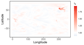
(a) $\mathrm{I}_{\rm fit}(L_{i},l_{j})$

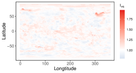
(b) $\mathrm{I}_{\rm uq}(L_{i},l_{j})$

Figure 5: (a) is the map of $\{\mathrm{I}_{\rm fit}(L_{i},l_{j})\}_{i=1,\ldots,I;j=1,\ldots,J}$ for the annual temperature with $R=7$. (b) is the map of $\{\mathrm{I}_{\rm uq}(L_{i},l_{j})\}_{i=1,\ldots,I;j=1,\ldots,J}$ for the annual temperature with $R^{\prime}=R=7$.

In addition to assessing goodness-of-fit and variability, we also compare basic statistical characteristics of our emulations to those of the simulations. Using the generated emulations, we replicate the procedures outlined in Fig. 1. Figs. S3(a), S3(b), and 6(a) exhibit patterns similar to those observed in Figs. 1(a)–1(c), respectively. Moreover, for each grid point, we compare the empirical distribution of $\{y_{SG,t}^{(r)}(L_{i},l_{j})\}_{t=1,\ldots,T;r=1,\ldots,R}$ to that of $\{y_{t}^{(r)}(L_{i},l_{j})\}_{t=1,\ldots,T;r=1,\ldots,R}$ by the Wasserstein distance (Santambrogio, 2015), which is denoted as $\mathrm{WD}_{S}(L_{i},l_{j})$ and shown in Fig. 6(b). Similarly, we calculate the Wasserstein distance between the empirical distribution of $\{y_{SG,t}^{(r)}(L_{i},l_{j})\}_{i=1,\ldots,I;j=1,\ldots,J;r=1,\ldots,R}$ and $\{y_{t}^{(r)}(L_{i},l_{j})\}_{i=1,\ldots,I;j=1,\ldots,J;r=1,\ldots,R}$ for each time point $t$, which is denoted as $\mathrm{WD}_{T}(t)$. The medians of $\{\mathrm{WD}_{S}(L_{i},l_{j})\}_{i=1,\ldots,I;j=1,\ldots,J}$ and $\{\mathrm{WD}_{T}(t)\}_{t=1,\ldots,T}$ are $0.066$ and $0.126$, respectively. These provide further evidence of the similarity between our emulations and the simulations.

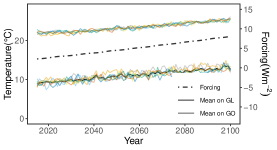
(a) Time series

(b) Wasserstein distance

Figure 6: Illustration of $R^{\prime}$ generated annual emulations. (a) shows annual temperature time series of emulations at GL and GO. (b) is the map of Wasserstein distance $\{\mathrm{WD}_{S}(L_{i},l_{j})\}_{i=1,\ldots,I;j=1,\ldots,J}$.

4.2 Monthly aggregated temperature

Let $\{y_{t}^{(r)}(L_{i},l_{j})\}_{i=1,\ldots,I;j=1,\ldots,J;t=1,\ldots,T;r=1,\ldots,R}$ represent the monthly aggregated temperature simulations with $T=1032$. In this subsection, we focus on the impact of increasing temporal resolution. We start by modeling the deterministic component, where $K_{M}$ harmonic terms are added in $m_{t}(L_{i},l_{j})$ to account for interannual trends. Based on BIC, the proportions of grid points selecting $K_{M}=1,\ldots,5$ are $0.5\%$, $16.2\%$, $33.3\%$, $33.2\%$ and $16.8\%$, respectively. For the sake of efficient storage and analysis, we choose $K_{M}=3$. By Jarque-Bera tests, the stochastic components at about $95.3\%$ grid points do not conform to a Gaussian distribution. Consequently, the index $\mathrm{I}_{\rm fit}$ is no longer an appropriate measure for assessing the goodness-of-fit of the SG (Castruccio et al., 2019). We give an intuitive comparison between the estimated $m_{t}$ and the ensemble mean, and the map of $\hat{\sigma}$ in Figs. S4(a) and S4(b), respectively. After obtaining the stochastic component, we apply the SHT (5) to reduce its dimension. By BIC as shown in Fig. S4(c), we choose $Q_{l}=36$ and $Q_{o}=70$ for the monthly data. These values are very close to the $Q$ values chosen for the annual data and remain unaffected by the increase in temporal resolution. Correspondingly, the estimate of $v(L_{i},l_{j})$ is also provided in Fig. S4(d), which has similar pattern and scale to Fig. 3(d).

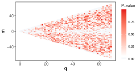
(a) Jarque-Bera test

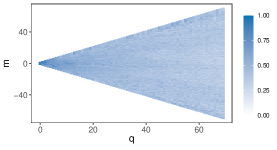
(b) $(\hat{\phi}_{1})_{q}^{m}$ for monthly data

Figure 7: (a) shows the $p$-values from Jarque-Bera tests of coefficients. Points with $p$-values less than $0.05$ reject the Gaussian assumption. (b) is the map of the estimated $\{(\phi_{1})_{q}^{m}\}_{q=0,\ldots,Q_{o}-1;m=-q,\ldots,q}$ for the monthly aggregated simulations.

Now, we assess the temporal dependence in the spectral domain using $(\tilde{s}_{t}^{(r)})_{q}^{m}$’s. From Fig. 7(a), only $42.6\%$ coefficients reject the Gaussianity and belong to $\mathcal{S}_{gh}$, although $\{Z_{t}^{(r)}(L_{i},l_{j})\}_{t=1,\ldots,T;r=1,\ldots,R}$ at most grid points are not Gaussian. It implies that the non-Gaussianity of monthly data is not severe. The proportions of $P=1,\ldots,5$ are $87.3\%$, $8.8\%$, $3.4\%$, and $0.3\%$ and $0.2\%$, respectively. Therefore, we choose $P=1$ for the monthly data and display the corresponding $(\hat{\phi}_{1})_{q}^{m}$ in Fig. 7(b). Compared with the $(\hat{\phi}_{1})_{q}^{m}$s for annual data in Fig. 4(a), those for monthly data have an obvious trend. That is, the lower the degree, the stronger the temporal correlation. The assessment of spatial dependence is easily performed by evaluating $\check{\mathbf{K}}$ with $(\check{s}_{t}^{(r)})_{q}^{m}$.

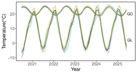
(a) Time series

(b) $\mathrm{I}_{\rm uq}(L_{i},l_{j})$

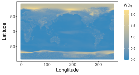
(c) $\mathrm{WD}_{S}(L_{i},l_{j})$

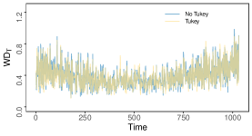
(d) $\mathrm{WD}_{T}(t)$

Figure 8: Performance of $R^{\prime}=7$ monthly emulations generated using the TGH transformation. (a) shows the monthly temperature time series of emulations at GL and GO, where the black curves are ensemble means of emulations. (b) and (c) are maps of $\{\mathrm{I}_{\rm uq}(L_{i},l_{j})\}_{i=1,\ldots,I;j=1,\ldots,J}$ and $\{\mathrm{WD}_{S}(L_{i},l_{j})\}_{i=1,\ldots,I;j=1,\ldots,J}$, respectively. (d) compares $\{\mathrm{WD}_{T}(t)\}_{t=1}^{T}$ of emulations generated with and without the TGH transformation.

Fig. 8 illustrates the performance of our SG, and its $R^{\prime}=7$ emulations. Intuitively, emulations in Fig. 8(a) have similar variability and pattern to those in Fig. 1(d). Moreover, Figs. S5(a) and S5(b) compare empirical distributions of emulations with those of simulations from different views, which can be measured using the Wasserstein distances $\mathrm{WD}_{S}$ and $\mathrm{WD}_{T}$, respectively. From Figs. 8(b) and 8(c), $\mathrm{I}_{\rm uq}$ values are close to $1$ and $\mathrm{WD}_{S}$ values are close to $0$ at most grid points. The proposed SG cannot perform well at the north pole and the Band regions because of the numerical instabilities of surface temperature in these regions. The medians of $\mathrm{I}_{\rm uq}$ in Fig. 8(b) and $\mathrm{WD}_{S}$ in Fig. 8(c) are $1.053$ and $0.117$, respectively. The values of $\mathrm{WD}_{T}$ are also small, especially at time points in the middle. The medians of $\mathrm{WD}_{T}$ for emulations with and without TGH are $0.370$ and $0.369$, respectively. Combining with results in Figs. S5(c) and S5(d), the SG without the TGH is comparable to that using the TGH. On the one hand, as we mentioned above, the monthly temperature may just be slightly skewed or heavy/light-tailed. On the other hand, the use of TGH may bring additional uncertainty.

4.3 Daily aggregated temperature

Now, we develop an SG for the daily aggregated temperature simulations with $T=31,390$. Analyzing such a vast amount of data presents a computational challenge. Therefore, we adopt a strategy similar to Huang et al. (2023) to perform inference only on data at years 2020, 2040, 2060, 2080, and 2100. The procedure of inference closely follows that of the monthly case. Therefore, we put the details of development to Section S4.3 of the Supplementary Materials and focus on assessing the performance of the emulations and a further exploration of data characteristics.

For the daily data, we choose $K_{D}=4$ and $P=1$. The choice of $K_{D}>K_{M}$ and the more structured and higher $(\hat{\phi}_{1})_{q}^{m}$ in Fig. S6(f) reflect the impact of the increased temporal resolution. The BIC in Fig. S6(c) helps us to choose $Q_{l}=36$ and $Q_{o}=68$. Using the results obtained from the previous analysis, we generate $R^{\prime}=7$ emulations for the daily temperature simulations. Their performance is examined by $\mathrm{I}_{\rm uq}$ and $\mathrm{WD}_{S}$ values shown in Figs. 9(a) and 9(b), respectively. As in the monthly case, the daily emulations exhibit challenges in accurately representing certain regions, notably the north pole and the Band regions. These regions display larger $\mathrm{I}_{\rm uq}$ values, indicating higher uncertainty. Additionally, they may deviate from the behavior observed in the simulations, as reflected by the larger $\mathrm{WD}_{S}$ values. Moreover, $\mathrm{WD}_{S}$ values are generally higher over land compared to ocean areas, which may be attributed to the complex non-stationary nature of the temperature on land.

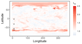
(a) $\mathrm{I}_{\rm uq}(L_{i},l_{j})$

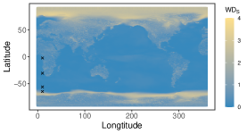
(b) $\mathrm{WD}_{S}(L_{i},l_{j})$

Figure 9: Performance of $R^{\prime}=7$ daily emulations. (a) and (b) are maps of $\{\mathrm{I}_{\rm uq}(L_{i},l_{j})\}_{i=1,\ldots,I;j=1,\ldots,J}$ and $\{\mathrm{WD}_{S}(L_{i},l_{j})\}_{i=1,\ldots,I;j=1,\ldots,J}$ for daily emulations. Points $\times$ represent four testing grid points TGL=$(-2.36,10.00)$, TGO=$(-30.63,10.00)$, TGN=$(-56.07,10.00)$, and TGB=$(-64.55,10.00)$.

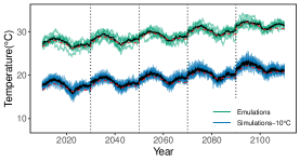
(a) TGL

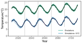
(b) TGO

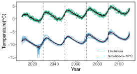
(c) TGN

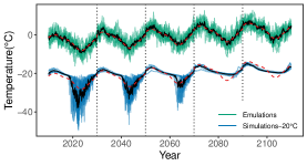
(d) TGB

Figure 10: Comparison of daily emulations and simulations at four testing grid points. The black solid curves are ensemble means for simulations and emulations. The red dashed curves are $\hat{m}_{t}$s.

We further explore these by intuitively displaying and comparing simulations and emulations at four testing grid points selected from the southern hemisphere with the same longitude in Fig. 10. TGL is a land point near the equator. In Fig. 10(a), temperature simulations on TGL exhibit larger variability but can be well replicated by the emulations. TGO is an ocean point in the middle latitudes. From Fig. 10(b), temperature simulations on TGO have smaller variability overall, with relatively larger variability at peaks and valleys of each year. These patterns can also be observed at emulations on TGO. TGN is also an ocean point in the middle latitudes, but very close to the Band region. In Fig. 10(c), some temperature simulations exhibit sudden drops at year 2020, which leads to an overestimate of $\hat{\sigma}(\rm TGN)$, and hence a relatively higher variability in the emulations. Despite this, with $\mathrm{I}_{\rm uq}(\rm TGN)=1.130$ and $\mathrm{WD}_{S}(\rm TGN)=0.117$, the abnormal drops do not significantly affect these indices. Both $\mathrm{I}_{\rm uq}$ and $\mathrm{WD}_{S}$ exhibit a certain tolerance to isolated “outliers”. TGB is an ocean point within the Band region. Compared with the scenarios in Fig. 10(c), temperature simulations at TGB display much more rapid and significant fluctuations at the years 2020, 2040, and 2060. In contrast, in years 2080 and 2100, the temperature simulations behave as other grid points on ocean with small variability. Simulations at the north pole region exhibit similar patterns. According to the explanation kindly provided by NCAR, these temperature fluctuations are caused by the way of data generation. Specifically, the surface temperature in simulations is the spatial average of the surface temperature of whatever medium is in the grid box, whether it is water, land, or sea ice. Grid points at Band and north pole regions undergo a dynamic transition, shifting back and forth between being partial sea ice and being open ocean. Consequently, sometimes we get the temperature of sea ice, and sometimes we get the temperature of the top layer of the ocean (or a mixture of the two). Emulations cannot capture these fluctuations, since we assume that $\hat{\sigma}$ remains constant over time. Even if they could, they would not mimic a real ESM for the surface temperature.

5 Conclusion and Future Work

In this paper, we presented an efficient SG for global temperature simulations from the newly published CESM2-LENS2. With at most $O(IJ+Q_{o}^{3})$ parameters to be stored, an unlimited number of emulations of size $O(IJT)$, even at a daily scale, can be generated to help with the investigation of climate internal variability. Such a saving of computational time and resources comes from the use of SHT, which expands data with $Q^{2}\ll IJ$ spherical harmonics and represents a practical low-rank approximation on the sphere. By customizing $Q$ values for grid points on land and ocean and leveraging the axial symmetry, the proposed SG can properly capture the complex non-stationary dependencies among different latitudes and land/ocean regions. To account for the non-Gaussian nature of the high-resolution time series, we introduced a modified TGH transformation into the SG. In our case study, we developed SGs based on $R=7$ annually, monthly and daily aggregated simulations, respectively. We evaluated the efficiency and accuracy of the proposed SG by comparing the generated emulations to the original simulations using various indexes and visual inspections.

A natural extension is to apply the proposed algorithms to hourly temperature simulations, which may exhibit even more pronounced skewness, kurtosis, and other intriguing characteristics. Additionally, the proposed algorithms are also available to other simulations with similar characteristics. Investigating regional climate change is also of paramount importance. On the one hand, climate change does not affect all regions equally. On the other hand, different regions have varying levels of vulnerability to climate change, e.g., extreme weather events, sea-level rise, or precipitation patterns. Local communities, governments, and businesses may be interested in how specific areas are being impacted so that they can adapt and plan for the future. Therefore, another possible extension is to build an SG for high-resolution climate simulations on a specific region.

Supplementary Materials

S1 Introduction

This documents supplements the main manuscript, providing more details about the CESM2-LENS2 data, inference process, derivation, validation, and results in case study.

S2 Supplement to Section 2

We further explores the characteristics of simulations with different temporal resolutions. Fig. S1 illustrates their skewness and kurtosis after detrending by ensemble means. For daily data, only temperature at years 2020, 2040, 2060, 2080, and 2100 are used. Kurtosis of monthly and daily data larger than $15$ are displayed as $15$ in Figs. S1(e) and S1(f) for better illustration. Note that the extents of both skew and heavy tail become severe with the increase of temporal resolution, especially for data near the north pole region and the band region below latitude $-60^{\circ}$, which is termed as Band region.

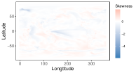
(a) Skewness of annual data

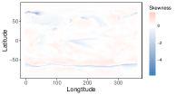
(b) Skewness of monthly data

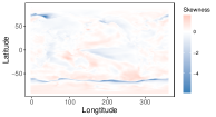
(c) Skewness of daily data

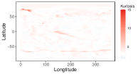
(d) Kurtosis of annual data

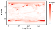
(e) Kurtosis of monthly data

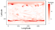
(f) Kurtosis of daily data

Figure S1: Skewness and kurtosis of annually, monthly, and daily aggregated detrended temperature simulations over globe.

S3 Supplement to Section 3

S3.1 Evaluation of parameters in the deterministic component

For writing simplicity, we take the annually aggregated temperature as an example to illustrate the inferential process, which follows previous works (Castruccio et al., 2014; Huang et al., 2023). First, we fix $\rho(L_{i},l_{j})$ so that Model (1) simplifies into an ordinary linear regression

$$y_{t}^{(r)}(L_{i},l_{j})=\mathbf{x}_{t}(L_{i},l_{j})^{\top}\bm{\beta}(L_{i},l_{j})+\sigma(L_{i},l_{j})Z_{t}^{(r)}(L_{i},l_{j}),\quad t=1,\ldots,T,$$

where $\mathbf{x}_{t}(L_{i},l_{j})=[1,x_{t},\{1-\rho(L_{i},l_{j})\}\sum_{s=1}^{\infty}\rho(L_{i},l_{j})^{s-1}x_{t-s}]^{\top}$, $\bm{\beta}(L_{i},l_{j})=[\beta_{0}(L_{i},l_{j}),\beta_{1}(L_{i},l_{j})$, $\beta_{2}(L_{i},l_{j})]^{\top}$, and $Z_{t}^{(r)}(L_{i},l_{j})$ is the white noise. By maximizing the log likelihood function $l_{\rho}\{\bm{\beta}(L_{i},l_{j})$, $\sigma^{2}(L_{i},l_{j})\}$, we get estimates of $\bm{\beta}(L_{i},l_{j})$ and $\sigma^{2}(L_{i},l_{j})$:

$$\hat{\bm{\beta}}_{\rho}(L_{i},l_{j})=\{\mathbf{X}(L_{i},l_{j})^{\top}\mathbf{X}(L_{i},l_{j})\}^{-1}\mathbf{X}(L_{i},l_{j})^{\top}\mathbf{y}^{(r)}(L_{i},l_{j}),$$

$$\hat{\sigma}_{\rho}^{2}(L_{i},l_{j})=T^{-1}\{\mathbf{y}^{(r)}(L_{i},l_{j})-\mathbf{X}(L_{i},l_{j})\hat{\bm{\beta}}(L_{i},l_{j})\}^{\top}\{\mathbf{y}^{(r)}(L_{i},l_{j})-\mathbf{X}(L_{i},l_{j})\hat{\bm{\beta}}(L_{i},l_{j})\},$$

where $\mathbf{X}(L_{i},l_{j})=[\mathbf{x}_{1}(L_{i},l_{j}),\ldots,\mathbf{x}_{T}(L_{i},l_{j})]^{\top}$ and $\mathbf{y}^{(r)}(L_{i},l_{j})=[y_{1}^{(r)}(L_{i},l_{j}),\ldots,y_{T}^{(r)}(L_{i},l_{j})]^{\top}$. Then, we combine the information from all ensembles to estimate $\hat{\rho}(L_{i},l_{j})$, which is achieved by maximizing the profile log likelihood:

$$l_{\rho}\{\hat{\bm{\beta}}_{\rho}(L_{i},l_{j}),\hat{\sigma}_{\rho}^{2}(L_{i},l_{j})\}\propto$$

$$\sum_{r=1}^{R}-\log[\mathbf{y}^{(r)\top}(L_{i},l_{j})\{\mathbf{I}_{T}-\mathbf{X}(L_{i},l_{j})(\mathbf{X}(L_{i},l_{j})^{\top}\mathbf{X}(L_{i},l_{j}))^{-1}\mathbf{X}(L_{i},l_{j})^{\top}\}\mathbf{y}^{(r)}(L_{i},l_{j})]$$

Finally, we evaluate the deterministic component with the estimated parameters $\hat{\bm{\beta}}(L_{i},l_{j})=\hat{\bm{\beta}}_{\hat{\rho}}(L_{i},l_{j})$ and $\hat{\sigma}^{2}(L_{i},l_{j})=\hat{\sigma}_{\hat{\rho}}^{2}(L_{i},l_{j})$.

S3.2 Structure derivation for $\tilde{\mathbf{K}}$ under the axial symmetry

In this subsection, we derive the structure of $\tilde{\mathbf{K}}$ under the assumption of axial symmetry. First, we expand $Z(L_{i},l_{j})=Z(\theta,\psi)$ with spherical harmonics as

$$Z(\theta,\psi) =\sum_{q=0}^{Q-1}\sum_{m=-q}^{q}H_{q}^{m}(\theta,\psi)s_{q}^{m}$$

$$=\sum_{q=0}^{Q-1}[\sum_{m=1}^{q}\{H_{q}^{m}(\theta,\psi)s_{q}^{m}+H_{q}^{-m}(\theta,\psi)s_{q}^{-m}\}+H_{q}^{0}(\theta,\psi)s_{q}^{0}]$$

$$=\sum_{q=0}^{Q-1}\{\sum_{m=1}^{q}F(q,m)+H_{q}^{0}(\theta,\psi)s_{q}^{0}\}.$$

With the closed-form

$$H_{q}^{m}(\theta,\psi)=\sqrt{\frac{2q+1}{4\pi}\frac{(q-m)!}{(q+m)!}}P_{q}^{m}(\cos\theta)\exp(\iota m\psi),$$

we have $H_{q}^{m}(\theta,\psi)=H_{q}^{m}(\theta,0)\exp(\iota m\psi)$. Moreover, $H_{q}^{-m}(\theta,0)=(-1)^{m}H_{q}^{m}(\theta,0)$ by $P_{q}^{-m}=(-1)^{m}\frac{(q-m)!}{(q+m)!}P_{q}^{m}$. Therefore,

$$F(q,m) =H_{q}^{m}(\theta,0)\exp(\iota m\psi)\{\Re(s_{q}^{m})+\iota\Im(s_{q}^{m})\}+H_{q}^{-m}(\theta,0)\exp(-\iota m\psi)(-1)^{m}\{\Re(s_{q}^{m})-\iota\Im(s_{q}^{m})\}$$

$$=H_{q}^{m}(\theta,0)\{\cos(m\psi)+\iota\sin(m\psi)\}(\tilde{s}_{q}^{m}+\iota\tilde{s}_{q}^{-m})$$

$$\quad+(-1)^{m}H_{q}^{-m}(\theta,0)\{\cos(m\psi)-\iota\sin(m\psi)\}(\tilde{s}_{q}^{m}-\iota\tilde{s}_{q}^{-m})$$

$$=H_{q}^{m}(\theta,0)\cos(m\psi)(\tilde{s}_{q}^{m}+\iota\tilde{s}_{q}^{-m})+(-1)^{m}H_{q}^{-m}(\theta,0)\iota\sin(m\psi)(\tilde{s}_{q}^{m}+\iota\tilde{s}_{q}^{-m})$$

$$\quad+H_{q}^{m}(\theta,0)\cos(m\psi)(\tilde{s}_{q}^{m}-\iota\tilde{s}_{q}^{-m})-(-1)^{m}H_{q}^{-m}(\theta,0)\iota\sin(m\psi)(\tilde{s}_{q}^{m}-\iota\tilde{s}_{q}^{-m})$$

$$=2H_{q}^{m}(\theta,0)\cos(m\psi)\tilde{s}_{q}^{m}-2(-1)^{m}H_{q}^{-m}(\theta,0)\sin(m\psi)\tilde{s}_{q}^{-m}.$$

Now, we calculate the covariance between $Z(\theta,\psi)$ and $Z(\theta^{\prime},\psi^{\prime})$:

$$\mathrm{E}\{Z(\theta,\psi)Z(\theta^{\prime},\psi^{\prime})\} =\sum_{q=1}^{Q-1}\sum_{q^{\prime}=1}^{Q-1}[\sum_{m=1}^{q}\sum_{m^{\prime}=1}^{q^{\prime}}\mathrm{E}\{F(q,m)F^{\prime}(q^{\prime},m^{\prime})\}+\mathrm{E}\{H_{q}^{0}(\theta,\psi)s_{q}^{0}H_{q^{\prime}}^{0}(\theta^{\prime},\psi^{\prime})s_{q^{\prime}}^{0}\}$$

$$\quad+\sum_{m^{\prime}=1}^{q^{\prime}}\mathrm{E}\{F^{\prime}(q^{\prime},m^{\prime})H_{q}^{0}(\theta,\psi)s_{q}^{0}\}+\sum_{m=1}^{q}\mathrm{E}\{F(q,m)H_{q^{\prime}}^{0}(\theta^{\prime},\psi^{\prime})s_{q^{\prime}}^{0}\}].$$

For the first term in bracket, we have

$$\frac{1}{4}\mathrm{E}\{F(q,m)F^{\prime}(q^{\prime},m^{\prime})\} =\mathrm{E}[\{H_{q}^{m}(\theta,0)\cos(m\psi)\tilde{s}_{q}^{m}-(-1)^{m}H_{q}^{-m}(\theta,0)\sin(m\psi)\tilde{s}_{q}^{-m}\}$$

$$\quad\{H_{q^{\prime}}^{m^{\prime}}(\theta^{\prime},0)\cos(m^{\prime}\psi^{\prime})\tilde{s}_{q^{\prime}}^{m^{\prime}}-(-1)^{m^{\prime}}H_{q^{\prime}}^{-m^{\prime}}(\theta^{\prime},0)\sin(m^{\prime}\psi^{\prime})\tilde{s}_{q^{\prime}}^{-m^{\prime}}\}]$$

$$=H_{q}^{m}(\theta,0)H_{q^{\prime}}^{m^{\prime}}(\theta^{\prime},0)\cos(m\psi)\cos(m^{\prime}\psi^{\prime})\mathrm{E}(\tilde{s}_{q}^{m}\tilde{s}_{q^{\prime}}^{m^{\prime}})$$

$$\quad-(-1)^{m^{\prime}}H_{q}^{m}(\theta,0)H_{q^{\prime}}^{-m^{\prime}}(\theta^{\prime},0)\cos(m\psi)\sin(m^{\prime}\psi^{\prime})\mathrm{E}(\tilde{s}_{q}^{m}\tilde{s}_{q^{\prime}}^{-m^{\prime}})$$

$$\quad-(-1)^{m}H_{q}^{-m}(\theta,0)H_{q^{\prime}}^{m^{\prime}}(\theta^{\prime},0)\sin(m\psi)\cos(m^{\prime}\psi^{\prime})\mathrm{E}(\tilde{s}_{q}^{-m}\tilde{s}_{q^{\prime}}^{m^{\prime}})$$

$$\quad+(-1)^{m+m^{\prime}}H_{q}^{-m}(\theta,0)H_{q^{\prime}}^{-m^{\prime}}(\theta^{\prime},0)\sin(m\psi)\sin(m^{\prime}\psi^{\prime})\mathrm{E}(\tilde{s}_{q}^{-m}\tilde{s}_{q^{\prime}}^{-m^{\prime}}).$$

To let the above equality only depend on $\theta$, $\theta^{\prime}$, and $|\psi-\psi^{\prime}|$, we need $\mathrm{E}(\tilde{s}_{q}^{m}\tilde{s}_{q^{\prime}}^{m^{\prime}})=\mathrm{E}(\tilde{s}_{q}^{-m}\tilde{s}_{q^{\prime}}^{-m^{\prime}})=k_{qq^{\prime}m}\delta_{m=m^{\prime}}\delta_{m>0}$. For the second term in bracket, we have

$$\mathrm{E}\{H_{q}^{0}(\theta,\psi)s_{q}^{0}H_{q^{\prime}}^{0}(\theta^{\prime},\psi^{\prime})s_{q^{\prime}}^{0}\}=H_{q}^{0}(\theta,0)H_{q^{\prime}}^{0}(\theta^{\prime},0)\mathrm{E}(s_{q}^{0}s_{q^{\prime}}^{0}),$$

which only depend on $\theta$ and $\theta^{\prime}$. For the third term in bracket, we have

$$\mathrm{E}\{F^{\prime}(q^{\prime},m^{\prime})H_{q}^{0}(\theta,\psi)s_{q}^{0}\} =2\mathrm{E}[\{H_{q^{\prime}}^{m^{\prime}}(\theta^{\prime},0)\cos(m^{\prime}\psi^{\prime})\tilde{s}_{q^{\prime}}^{m^{\prime}}-(-1)^{m^{\prime}}H_{q^{\prime}}^{-m^{\prime}}(\theta^{\prime},0)\sin(m^{\prime}\psi^{\prime})\tilde{s}_{q^{\prime}}^{-m^{\prime}}\}H_{q}^{0}(\theta,\psi)s_{q}^{0}]$$

$$=2H_{q^{\prime}}^{m^{\prime}}(\theta^{\prime},0)H_{q}^{0}(\theta,\psi)\cos(m^{\prime}\psi^{\prime})\mathrm{E}(\tilde{s}_{q^{\prime}}^{m^{\prime}}s_{q}^{0})$$

$$\quad-2(-1)^{m^{\prime}}H_{q^{\prime}}^{-m^{\prime}}H_{q}^{0}(\theta,\psi)(\theta^{\prime},0)\sin(m^{\prime}\psi^{\prime})\mathrm{E}(\tilde{s}_{q^{\prime}}^{-m^{\prime}}s_{q}^{0}).$$

To let the above equality only depend on $\theta$, $\theta^{\prime}$, and $|\psi-\psi^{\prime}|$, we need $\mathrm{E}(\tilde{s}_{q^{\prime}}^{m^{\prime}}s_{q}^{0})=\mathrm{E}(\tilde{s}_{q^{\prime}}^{-m^{\prime}}s_{q}^{0})=0$, where $m$ and $m^{\prime}>1$. In general, to satisfy the assumption of axial symmetry, we should let $\mathrm{E}(\tilde{s}_{q}^{m}\tilde{s}_{q^{\prime}}^{m^{\prime}})=\mathrm{E}(\tilde{s}_{q}^{-m}\tilde{s}_{q^{\prime}}^{-m^{\prime}})=k_{qq^{\prime}m}\delta_{m=m^{\prime}}\delta{m\geq 0}$.

We calculate the number of non-zero elements in $\tilde{\mathbf{K}}$. When $m=0$, $\forall q,q^{\prime}=0,1,\ldots,Q-1$, the $(q^{2}+q+1,q^{\prime 2}+q^{\prime}+1)$th element of $\tilde{\mathbf{K}}$ is non-zero. Therefore, $Q^{2}$ non-zero elements for $m=0$. When $m\geq 1$, $\forall q,q^{\prime}=m,\ldots,Q-1$, the $(q^{2}+q+m+1,q^{\prime 2}+q^{\prime}+m+1)$th and $(q^{2}+q-m+1,q^{\prime 2}+q^{\prime}-m+1)$th elements of $\tilde{\mathbf{K}}$ are non-zero. Therefore, $2(Q-m)^{2}$ non-zero-elements for $m\geq 1$. The total number of non-zero elements in $\tilde{\mathbf{K}}$ is $Q^{2}+2(Q-1)^{2}+2(Q-2)^{2}+\ldots 2=2Q^{3}/3+Q/3$.

However, not all non-zero elements need to be stored. Some element values are repeated. For $m=0$, only $Q(Q+1)/2$ elements of $\tilde{\mathbf{K}}$ need to be stored, which are indexed by $(q^{2}+q+1,q^{\prime 2}+q^{\prime}+1)$ with $q=0,\ldots,Q-1$ and $q^{\prime}=q,\ldots,Q-1$. For $m\geq 1$, $(Q-m)(Q-m+1)/2$ elements indexed by $(q^{2}+q+m+1,q^{\prime 2}+q^{\prime}+m+1)$ or $(q^{2}+q-m+1,q^{\prime 2}+q^{\prime}-m+1)$ need to be stored, where $q=m,\ldots,Q-1$ and $q^{\prime}=q,\ldots,Q-1$. Therefore, the total number of elements to be memorized is $Q(Q+1)/2+(Q-1)(Q-1+1)/2+\ldots,1\times 2/2=Q^{3}/6+Q^{2}/2+Q/3$.

S3.3 Validation of diagonal matrix $\Phi_{p}$

We briefly validate the assumption of diagonal matrices $\{\Phi_{p}\}_{p=1}^{P}$, where $P=1$ is obtained by the inference in our case study. That is, we assume that the cross-correlation between elements of $\check{\mathbf{s}}_{t}$ ($\tilde{\mathbf{s}}_{t}$ for the annual data) can be neglected. The detailed procedure of validation is as follows. First, we fit any two time series $(\check{s}_{t})_{q}^{m}$ and $(\check{s}_{t})_{q^{\prime}}^{m^{\prime}}$ with their respective AR($1$) models, and obtain their residuals. Then, we calculate the $p$-values for the first temporal lag of the cross-correlation between these two residuals. We put the result in the $(q^{2}+q+m+1,{q^{\prime}}^{2}+q^{\prime}+m^{\prime}+1)$th element of matrix $\mathbf{PV}\in\mathbb{R}^{Q^{2}\times Q^{2}}$. Fig. S2 shows parts of $\mathbf{PV}$ matrices for annual and monthly data. For most pairs of $(\check{s}_{t})_{q}^{m}$ and $(\check{s}_{t})_{q^{\prime}}^{m^{\prime}}$, especially those with higher degrees, there is not enough evidence to conclude that a significant auto-correlation exists and the residuals are approximately independent. The proportions of $p$-values larger than $0.05$ are almost $1$ for all scales.

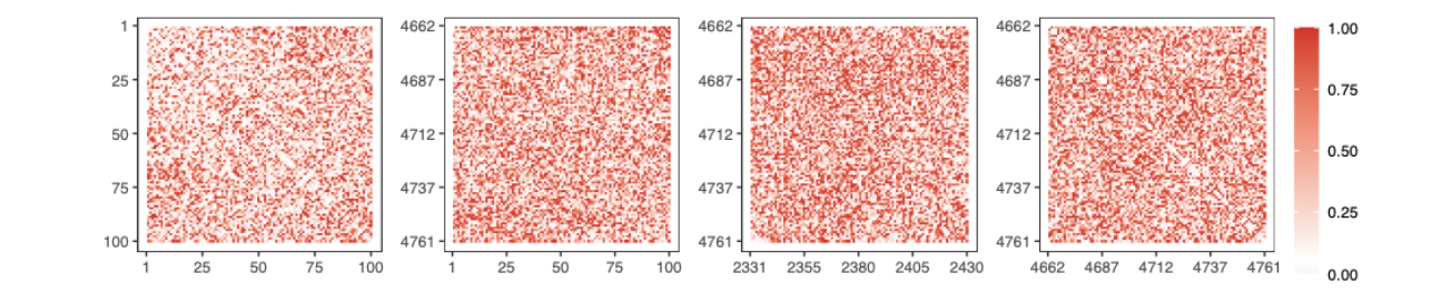
(a) Annual

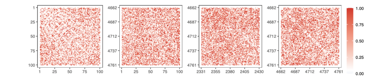
(b) Monthly

Figure S2: $P$-values of the first temporal lag of the cross-correlation for annual and monthly data.

S3.4 Evaluation of parameters in the modified TGH transformation

For a time series $\{\tilde{s}_{t}\}_{t=1}^{T}$ satisfying a TGH auto-regressive model, we can estimate the parameters $\bm{\mu}_{1}=(\omega,g,h)^{\top}$ and $\bm{\mu}_{2}=(\phi_{1},\ldots,\phi_{P})^{\top}$ by maximizing the following log-likelihood function (Yan and Genton, 2019):

$$\mathcal{L}_{T}(\bm{\mu}_{1},\bm{\mu}_{2};\{\tilde{s}_{t}\}_{t=1}^{T}) =f(\ddot{s}_{1,\bm{\mu}_{1}})+f(\ddot{s}_{2,\bm{\mu}_{1}}|\ddot{s}_{1,\bm{\mu}_{1}})+\cdots+f(\ddot{s}_{T,\bm{\mu}_{1}}|\ddot{s}_{T-1,\bm{\mu}_{1}},\ldots,\ddot{s}_{T-P,\bm{\mu}_{1}})$$

$$-T\log(\omega)-\frac{h}{2}\sum_{t=1}^{T}\ddot{s}_{t,\bm{\mu}_{1}}^{2}-\sum_{t=1}^{T}\log[\exp(g\ddot{s}_{t,\bm{\mu}_{1}})+\frac{h}{g}\{\exp(g\ddot{s}_{t,\bm{\mu}_{1}})-1\}\ddot{s}_{t,\bm{\mu}_{1}}],$$

where $f(\cdot|\cdot)$ is the conditional log-likelihood for the Gaussian AR($P$) process $\check{s}$ and $\ddot{s}_{t,\bm{\mu}_{1}}=\tau_{g,h}^{-1}\{\tilde{s}_{t}/\omega\}$.

For $(q,m)\in\mathcal{S}_{g,h}$, the estimate of $(\bm{\mu}_{1})_{q}^{m}$ and $(\bm{\mu}_{2})_{q}^{m}$ is the maximizer of $\sum_{r=1}^{R}\mathcal{L}_{T}(\cdot,\cdot;\{(\tilde{s}_{t}^{(r)})_{q}^{m}\}_{t=1}^{T})$, which contains information of all $R$ members. Then, $\lambda_{q}^{m}$ can be evaluated by $\mathrm{sd}\{(\tilde{s}_{t}^{(r)})_{q}^{m}\}/\mathrm{sd}\{(\ddot{s}_{t}^{(r)})_{q}^{m}\}$, where $\mathrm{sd}$ is the calculation of standard deviation over $t$ and $r$, and $(\check{s}_{t}^{(r)})_{q}^{m}=\lambda_{q}^{m}(\ddot{s}_{t}^{(r)})_{q}^{m}$. The value of $P$ can be chosen by using $\check{\mathrm{BIC}}_{q}^{m}(P)=-2\sum_{r=1}^{R}\mathcal{L}_{T}(\bm{\mu}_{1},\bm{\mu}_{2};\{(\tilde{s}_{t}^{(r)})_{q}^{m}\}_{t=1}^{T})+(P+3)\log\{R(T-P)\}$. These computations are expensive due to the non-analytic form of $\tau_{g,h}^{-1}$. Therefore, we follow Xu and Genton (2015) to find a maximum approximated likelihood estimator (MALE) by approximating $\tau_{g,h}^{-1}$ with a piecewise linear function. It significantly reduces the computational burden and takes only $O(T)$ computational time. For $(q,m)$ in the complementary set of $\mathcal{S}_{gh}$, we set $(\check{s}_{t}^{(r)})_{q}^{m}=(\tilde{s}_{t}^{(r)})_{q}^{m}$, $\bm{\mu}_{1}=\mathbf{0}$, $\lambda_{q}^{m}=1$, and evaluate $\bm{\mu}_{2}$ by VAR($P$).

S3.5 Algorithm for developing SG

This subsection provides a summary for procedures of developing SGs in Algorithm S1, which supplements to Section 3.3.

Algorithm S1 Construct an SG for CESM2-LENS2

0:  $\{y_{t}^{(r)}(L_{i},l_{j})\}_{t=1,\ldots,T;i=1,\ldots,I;j=1,\ldots,J;r=1,\ldots,R}$, $K$, $Q_{l}$, $Q_{o}$, $P$, $\mathbf{A}^{-1}\in\mathbb{R}^{Q_{o}^{2}\times Q_{o}^{2}}$

0:   For each grid point $(L_{i},l_{j})$, $i=1,\ldots,I$ and $j=1,\ldots,J$: 1) evaluate parameters $\rho(L_{i},l_{j})$, $\beta_{0}(L_{i},l_{j})$, $\beta_{1}(L_{i},l_{j})$, $\beta_{2}(L_{i},l_{j})$, $a_{1}(L_{i},l_{j})$,…, $a_{K}(L_{i},l_{j})$, $b_{1}(L_{i},l_{j})$,…, $b_{K}(L_{i},l_{j})$ in $m_{t}(L_{i},l_{j})$ and $\sigma(L_{i},l_{j})$ by the method in Section 3.1. 2) for each time point $t$, calculate $m_{t}(L_{i},l_{j})$ by plugging evaluated parameters into its expression, $t=1,\ldots,T$. 3) for each ensemble $r$, obtain the stochastic component $\{Z_{t}^{(r)}(L_{i},l_{j})\}_{t=1}^{T}$ by detrending and rescaling $\{y_{t}^{(r)}(L_{i},l_{j})\}_{t=1}^{T}$ with $m_{t}(L_{i},l_{j})$ and $\sigma(L_{i},l_{j})$, respectively, $r=1,\ldots,R$.

0:   1) For each ensemble $r$ and time point $t$, perform SHT on $\{Z_{t}^{(r)}(L_{i},l_{j})\}_{i=1,\ldots,I;j=1,\ldots,J}$ to obtain coefficients $\{(s_{t}^{(r)})_{q}^{m}\}_{q=0,\ldots,Q_{o}-1;m=-q,\ldots,q}$ and standard deviation $v(L_{i},l_{j})$. 2) Transform the complex-valued coefficient $(s_{t}^{(r)})_{q}^{m}$ to be the real-valued one $(\tilde{s}_{t}^{(r)})_{q}^{m}$ with $\mathbf{A}^{-1}$. 3) Evaluate the temporal dependence structure. For each $(q,m)$, test the Gaussianity of $\{(\tilde{s}_{t}^{(r)})_{q}^{m}\}_{t=1,\ldots,T;r=1,\ldots,R}$ and find the set $\mathcal{S}_{gh}$. Then, for $(q,m)\in\mathcal{S}_{gh}$, find the MALE of parameters $\omega_{q}^{m}$, $g_{q}^{m}$, $h_{q}^{m}$ and $\lambda_{q}^{m}$ in TGH transformation and $(\phi_{1})_{q}^{m},\ldots,(\phi_{P})_{q}^{m}$ in auto-regressive model using method in Section 3.2.2. Meanwhile, obtain $\{(\check{s}_{t}^{(r)})_{q}^{m}\}_{t=1,\ldots,T;r=1,\ldots,R}$. 4) Evaluate the spatial dependence structure. Empirically estimate the covariance matrix $\check{\mathbf{K}}$. That is, estimate $\check{k}_{qq^{\prime}m}$ with

$$(2RT)^{-1}\sum_{r=1}^{R}\sum_{t=1}^{T}\{(\check{s}_{t}^{(r)})_{q}^{m}(\check{s}_{t}^{(r)})_{q^{\prime}}^{m}+(\check{s}_{t}^{(r)})_{q}^{-m}(\check{s}_{t}^{(r)})_{q^{\prime}}^{-m}\}$$

0:  $\rho(L_{i},l_{j})$, $\beta_{0}(L_{i},l_{j})$, $\beta_{1}(L_{i},l_{j})$, $\beta_{2}(L_{i},l_{j})$, $a_{1}(L_{i},l_{j})$,…, $a_{K}(L_{i},l_{j})$, $b_{1}(L_{i},l_{j})$,…, $b_{K}(L_{i},l_{j})$, $\sigma(L_{i},l_{j})$, $v(L_{i},l_{j})$, $\lambda_{q}^{m}$, $\omega_{q}^{m}$, $g_{q}^{m}$, $h_{q}^{m}$, $(\phi_{1})_{q}^{m},\ldots,(\phi_{P})_{q}^{m}$, $\check{\mathbf{K}}$, $i=1,\ldots,I$, $j=1,\ldots,J$, $q=0,\ldots,Q_{o}-1$, $m=-q,\ldots,q$.

S4 Supplement to Section 4

S4.1 Annually aggregated temperature

This subsection illustrates the ensemble mean and standard error of the generated annual emulations. Plots in Fig. S3 have similar pattern to those in Figs. 1(a) and 1(b).

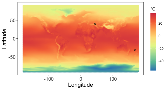
(a) $\bar{y}_{SG,9}$

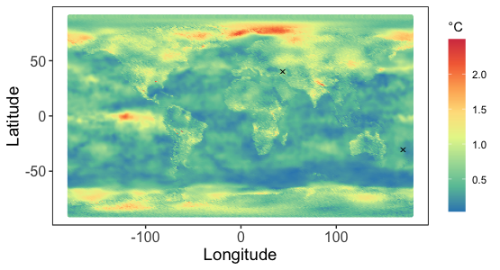
(b) $y_{SG,9}^{\rm sd}$

Figure S3: Illustration of $R^{\prime}$ generated annual emulations. (a) and (b) are maps of ensemble mean and standard deviation of the annual emulations at year 2023.

S4.2 Monthly aggregated temperature

Assume that $y_{t}^{(r)}(L_{i},l_{j})$ represents the temperature at grid point $(L_{i},l_{j})$, time point $t$ and ensemble $r$. Remember that the stochastic components at about $95\%$ grid points reject the Gaussian assumption and the index $\mathrm{I}_{\rm fit}$ is no longer proper to measure the goodness-of-fit of the SG. Therefore, we randomly choose a time point $105$ and intuitively compare the difference between $\hat{m}_{105}$ and the ensemble mean at $t=105$ in Fig. S4(a). The proposed SG can fit most regions well except for two pole and the Band regions because of the numerical instabilities. We also show the map of $\hat{\sigma}(L_{i},l_{j})$ in Fig. S4(b) and compare it with that in Fig. 3(b). They have similar pattern but the variation in monthly case is larger, since the monthly data have larger scale. Figs. S4(c) and S4(d) give more details about the SHT of monthly data.

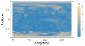
(a) $|\hat{m}_{105}(L_{i},l_{j})-\bar{y}_{105}(L_{i},l_{j})|$

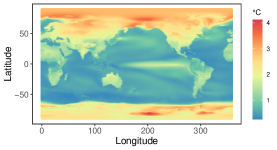
(b) $\hat{\sigma}(L_{i},l_{j})$

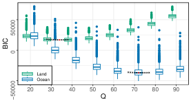
(c) BIC

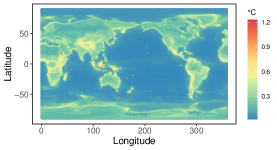
(d) $\hat{v}(L_{i},l_{j})$

Figure S4: (a) shows the gap between the estimated mean and ensemble mean of the monthly aggregated temperature simulations at September, 2023. (b) is the map of the estimated standard deviation $\hat{\sigma}(L_{i},l_{j})$ for the monthly aggregated temperature. (c) are boxplots of $\{\mathrm{BIC}_{*,t}^{(r)}(Q)\}_{r=1,\ldots,R;t=1,\ldots,T}$ for the monthly temperature against different values of $Q$, where $*$ takes “l” and “o”. Points $\times$ show median of BIC values. Red Points $\times$ indicate the minimum BIC medians. (d) is the map of $\hat{v}(L_{i},l_{j})$ for the monthly data.

We generate $R^{\prime}=7$ monthly emulations. Figs. S5(a) and S5(b) compare their empirical distributions with those of simulations, which can be measured using the Wasserstein distances $\mathrm{WD}_{S}$ and $\mathrm{WD}_{T}$, respectively. Moreover, we generate $R^{\prime}=7$ monthly emulations without using the modified TGH transformation for comparison. Their corresponding $\mathrm{I}_{\rm uq}$ and $\mathrm{WD}_{S}$ values are displayed in Figs. S5(c) and S5(d) with medians $1.053$ and $0.119$, respectively.

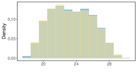
(a) $\{y_{t}^{(r)}(\rm GO)\}_{t,r}$ and $\{y_{SG,t}^{(r)}(\rm GO)\}_{t,r}$

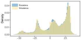
(b) $\{y_{555}^{(r)}(L_{i},l_{j})\}_{i,j,r}$ and $\{y_{SG,555}^{(r)}(L_{i},l_{j})\}_{i,j,r}$

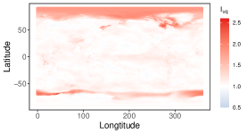
(c) $\mathrm{I}_{\rm uq}$

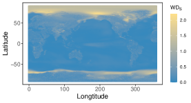
(d) $\mathrm{WD}_{S}$

Figure S5: (a) displays the histogram of $\{y_{t}^{(r)}(\mathrm{GO})\}_{t=1,\ldots,T;r=1,\ldots,R}$, and compares it with that of $\{y_{SG,t}^{(r)}(\mathrm{GL})\}_{t=1,\ldots,T;r=1,\ldots,R}$. (b) displays histograms of $\{y_{555}^{(r)}(L_{i},l_{j})\}_{i=1,\ldots,I;j=1,\ldots,J;r=1,\ldots,R}$ and $\{y_{SG,555}^{(r)}(L_{i},l_{j})\}_{i=1,\ldots,I;j=1,\ldots,J;r=1,\ldots,R}$. (c) and (d) are maps of $\{\mathrm{I}_{\rm uq}(L_{i},l_{j})\}_{i=1,\ldots,I;j=1,\ldots,J}$ and $\{\mathrm{WD}_{S}(L_{i},l_{j})\}_{i=1,\ldots,I;j=1,\ldots,J}$ for the monthly emulations generated without using TGH transformation, respectively.

S4.3 Daily aggregated temperature

This subsection supplements the case study of daily aggregated temperature simulations. Now, assume that $y_{t}^{(r)}(L_{i},l_{j})$ is the temperature at grid point $(L_{i},l_{j})$, day $t$ after year 2014, and ensemble $r$. In the deterministic component of daily temperature data, we choose $K_{D}=4$ using the BIC. Specifically, the proportions of grid points favoring $K_{D}=1$ through $K_{D}=5$ are $0.4\%$, $8.5\%$, $26.7\%$, $35.3\%$, and $29.1\%$, respectively. In Fig. S6(a), we intuitively compare the difference between $\hat{m}_{474}$ and the ensemble mean at $t=474$, which is a randomly chosen time point. There is a larger gap on land. It may result in the larger variation and uncertainty of temperature on land. The map of $\{\hat{\sigma}(L_{i},l_{j})\}_{i=1,\ldots,I;j=1,\ldots,J;t=1,\ldots,T;r=1,\ldots,R}$ is illustrated in Fig. S6(b), which has similar pattern to those of annual and monthly data but with larger scale.

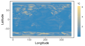
(a) $|\hat{m}_{474}(L_{i},l_{j})-\bar{y}_{474}(L_{i},l_{j})|$

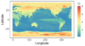
(b) $\hat{\sigma}(L_{i},l_{j})$

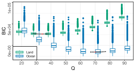
(c) BIC

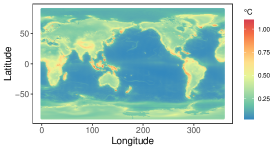
(d) $\hat{v}(L_{i},l_{j})$

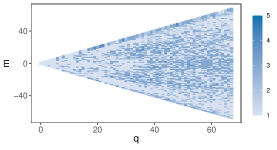
(e) BIC

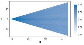
(f) $(\hat{\phi}_{1})_{q}^{m}$ for daily data

Figure S6: (a) shows the gap between the estimated mean and ensemble mean of the daily aggregated temperature simulations at 13rd September, 2023. (b) is the map of the estimated standard deviation $\hat{\sigma}(L_{i},l_{j})$ for the daily aggregated temperature. (c) are boxplots of $\{\mathrm{BIC}_{*,t}^{(r)}(Q)\}_{r=1,\ldots,R;t=1,\ldots,T}$ for the daily temperature under different values of $Q$, where $*$ takes l and o. Points $\times$ show median of BIC values. Red Points $\times$ indicate the minimum BIC medians. (d) is the map of $\hat{v}(L_{i},l_{j})$ for the daily data. (e) shows the order of $P$ selected by BIC in the TGH auto-regressive model. (f) is the map of the estimated $\{(\phi_{1})_{q}^{m}\}_{q=0,\ldots,Q_{o}-1;m=-q,\ldots,q}$ for the daily aggregated simulations.

After removing the deterministic components, we investigate the stochastic component. The BIC in Fig. S6(c) helps us to choose $Q_{l}=36$ and $Q_{o}=68$. Fig. S6(d) presents the corresponding $\hat{v}(L_{i},l_{j})$. Jarque-Bera tests reveal that over $98\%$ of grid points reject the Gaussian assumption in the spatial domain. The non-Gaussianity is then carried over to the spectral domain through the SHT, with about $56.7\%$ coefficients rejecting the Gaussian assumption. Moreover, lower-degree coefficients exhibit more pronounced skewness and heavier tails. For example, the skewness and kurtosis of $\{(\tilde{s}_{t}^{(r)})_{0}^{0}\}_{t=1,\ldots,T;r=1,\ldots,R}$ is $0.18$ and $3.07$, respectively. However, after applying the TGH transformation, these statistics of $\{(\check{s}_{t}^{(r)})_{0}^{0}\}_{t=1,\ldots,T;r=1,\ldots,R}$ improve to $0.02$ and $3.02$, respectively. In Fig. S6(e), the proportions of coefficients choosing $P=1,\ldots,5$ are $55.5\%$, $7.4\%$, $35.5\%$, $1.6\%$, and $0.0\%$, respectively. Most coefficients at lower degree, which is more influential, opt for $P=1$. Therefore, $P=1$ is ultimately selected for the daily data. In Fig. S6(f), the evaluation of $(\hat{\phi}_{1})_{q}^{m}$ reveal a more structured and highly correlated pattern compared to the results in Fig. 7(b) for the monthly data.

References

- Baker et al. (2017) Baker, A. H., Xu, H., Hammerling, D. M., Li, S., and Clyne, J. P. (2017), “Toward a multi-method approach: Lossy data compression for climate simulation data,” in International Conference on High Performance Computing, Springer, pp. 30–42.
- Banerjee et al. (2008) Banerjee, S., Gelfand, A. E., Finley, A. O., and Sang, H. (2008), “Gaussian predictive process models for large spatial data sets,” Journal of the Royal Statistical Society: Series B (Statistical Methodology), 70, 825–848.
- Bolin et al. (2023) Bolin, D., Simas, A. B., and Xiong, Z. (2023), “Covariance–based rational approximations of fractional SPDEs for computationally efficient Bayesian inference,” Journal of Computational and Graphical Statistics, 0, 1–11.
- Branstator and Teng (2010) Branstator, G. and Teng, H. (2010), “Two limits of initial-value decadal predictability in a CGCM,” Journal of Climate, 23, 6292–6311.
- Castruccio and Genton (2018) Castruccio, S. and Genton, M. G. (2018), “Principles for statistical inference on big spatio-temporal data from climate models,” Statistics & Probability Letters, 136, 92–96.
- Castruccio and Guinness (2017) Castruccio, S. and Guinness, J. (2017), “An evolutionary spectrum approach to incorporate large-scale geographical descriptors on global processes,” Journal of the Royal Statistical Society: Series C (Applied Statistics), 66, 329–344.
- Castruccio et al. (2019) Castruccio, S., Hu, Z., Sanderson, B., Karspeck, A., and Hammerling, D. (2019), “Reproducing internal variability with few ensemble runs,” Journal of Climate, 32, 8511–8522.
- Castruccio et al. (2014) Castruccio, S., McInerney, D. J., Stein, M. L., Crouch, F. L., Jacob, R. L., and Moyer, E. J. (2014), “Statistical emulation of climate model projections based on precomputed GCM runs,” Journal of Climate, 27, 1829–1844.
- Castruccio and Stein (2013) Castruccio, S. and Stein, M. L. (2013), “Global space-time models for climate ensembles,” The Annals of Applied Statistics, 1593–1611.
- Chang et al. (2014) Chang, W., Haran, M., Olson, R., and Keller, K. (2014), “Fast dimension-reduced climate model calibration and the effect of data aggregation,” The Annals of Applied Statistics, 8, 649–673.
- Cressie and Johannesson (2008) Cressie, N. and Johannesson, G. (2008), “Fixed rank kriging for very large spatial data sets,” Journal of the Royal Statistical Society: Series B (Statistical Methodology), 70, 209–226.
- Datta et al. (2016) Datta, A., Banerjee, S., Finley, A. O., and Gelfand, A. E. (2016), “Hierarchical nearest-neighbor Gaussian process models for large geostatistical datasets,” Journal of the American Statistical Association, 111, 800–812.
- Dong et al. (2023) Dong, C., Peings, Y., and Magnusdottir, G. (2023), “Regulation of Southwestern United States precipitation by non-ENSO teleconnections and the impact of the background flow,” Journal of Climate, 1–38.
- Eyring et al. (2016) Eyring, V., Bony, S., Meehl, G. A., Senior, C. A., Stevens, B., Stouffer, R. J., and Taylor, K. E. (2016), “Overview of the Coupled Model Intercomparison Project Phase 6 (CMIP6) experimental design and organization,” Geoscientific Model Development, 9, 1937–1958.
- Furrer and Sain (2010) Furrer, R. and Sain, S. R. (2010), “spam: A sparse matrix R package with emphasis on MCMC methods for Gaussian Markov random fields,” Journal of Statistical Software, 36, 1–25.
- Guinness (2021) Guinness, J. (2021), “Gaussian process learning via Fisher scoring of Vecchia’s approximation,” Statistics and Computing, 31, 25.
- Guinness and Hammerling (2018) Guinness, J. and Hammerling, D. (2018), “Compression and conditional emulation of climate model output,” Journal of the American Statistical Association, 113, 56–67.
- Hu and Castruccio (2021) Hu, W. and Castruccio, S. (2021), “Approximating the internal variability of bias-corrected global temperature projections with spatial stochastic generators,” Journal of Climate, 34, 8409–8418.
- Huang et al. (2023) Huang, H., Castruccio, S., Baker, A. H., and Genton, M. G. (2023), “Saving storage in climate ensembles: A model-based stochastic approach (with discussion),” Journal of Agricultural, Biological and Environmental Statistics, 28, 324–344.
- Jarque and Bera (1987) Jarque, C. M. and Bera, A. K. (1987), “A test for normality of observations and regression residuals,” International Statistical Review, 55, 163–172.
- Jeong et al. (2018) Jeong, J., Castruccio, S., Crippa, P., and Genton, M. G. (2018), “Reducing storage of global wind ensembles with stochastic generators,” The Annals of Applied Statistics, 12, 490–509.
- Jeong et al. (2017) Jeong, J., Jun, M., and Genton, M. (2017), “Spherical process models for global spatial statistics,” Statistical Science, 32, 501–513.
- Jeong et al. (2019) Jeong, J., Yan, Y., Castruccio, S., and Genton, M. G. (2019), “A stochastic generator of global monthly wind energy with Tukey g-and-h autoregressive processes,” Statistica Sinica, 29, 1105–1126.
- Jones (1963) Jones, R. H. (1963), “Stochastic processes on a sphere,” The Annals of Mathematical Statistics, 34, 213–218.
- Jun and Stein (2008) Jun, M. and Stein, M. (2008), “Nonstationary covariance models for global data,” The Annals of Applied Statistics, 2, 1271–1289.
- Katzfuss (2017) Katzfuss, M. (2017), “A multi-resolution approximation for massive spatial datasets,” Journal of the American Statistical Association, 112, 201–214.
- Kaufman et al. (2008) Kaufman, C. G., Schervish, M. J., and Nychka, D. W. (2008), “Covariance tapering for likelihood-based estimation in large spatial data sets,” Journal of the American Statistical Association, 103, 1545–1555.
- Kay et al. (2022) Kay, J. E., DeRepentigny, P., Holland, M. M., Bailey, D. A., DuVivier, A. K., Blanchard-Wrigglesworth, E., Deser, C., Jahn, A., Singh, H., Smith, M. M., et al. (2022), “Less surface sea ice melt in the CESM2 improves Arctic sea ice simulation with minimal non-polar climate impacts,” Journal of Advances in Modeling Earth Systems, 14, e2021MS002679.
- Kay et al. (2015) Kay, J. E., Deser, C., Phillips, A., Mai, A., Hannay, C., Strand, G., Arblaster, J. M., Bates, S., Danabasoglu, G., Edwards, J., et al. (2015), “The Community Earth System Model (CESM) large ensemble project: A community resource for studying climate change in the presence of internal climate variability,” Bulletin of the American Meteorological Society, 96, 1333–1349.
- Kennedy and O’Hagan (2001) Kennedy, M. C. and O’Hagan, A. (2001), “Bayesian calibration of computer models,” Journal of the Royal Statistical Society: Series B (Statistical Methodology), 63, 425–464.
- López-Pintado and Romo (2009) López-Pintado, S. and Romo, J. (2009), “On the concept of depth for functional data,” Journal of the American statistical Association, 104, 718–734.
- Lorenz (1963) Lorenz, E. N. (1963), “Deterministic nonperiodic flow,” Journal of Atmospheric Sciences, 20, 130–141.
- Muñoz et al. (2023) Muñoz, S. E., Dee, S. G., Luo, X., Haider, M. R., O’Donnell, M., Parazin, B., and Remo, J. W. F. (2023), “Mississippi River low-flows: context, causes, and future projections,” Environmental Research: Climate, 2, 031001.
- Nychka et al. (2015) Nychka, D., Bandyopadhyay, S., Hammerling, D., Lindgren, F., and Sain, S. (2015), “A multiresolution Gaussian Process model for the analysis of large spatial datasets,” Journal of Computational and Graphical Statistics, 24, 579–599.
- Oakley and O’Hagan (2002) Oakley, J. E. and O’Hagan, A. (2002), “Bayesian inference for the uncertainty distribution of computer model outputs,” Biometrika, 89, 769–784.
- Oakley and O’Hagan (2004) — (2004), “Probabilistic sensitivity analysis of complex models: a Bayesian approach,” Journal of the Royal Statistical Society: Series B (Statistical Methodology), 66, 751–769.
- Oceanic and Administration (2022) Oceanic, N. and Administration, A. (2022), “NOAA celebrates 200 years of science, service, and stewardship,” Revised October 24, 2022.
- O’Neill et al. (2014) O’Neill, B., Kriegler, E., Riahi, K., Ebi, K., Hallegatte, S., Carter, T., Mathur, R., and Vuuren, D. (2014), “A new scenario framework for climate change research: The concept of Shared Socioeconomic Pathways,” Climatic Change, 122, 401–414.
- Riahi et al. (2017) Riahi, K., van Vuuren, D. P., Kriegler, E., and et al. (2017), “The Shared Socioeconomic Pathways and their energy, land use, and greenhouse gas emissions implications: An overview,” Global Environmental Change, 42, 153–168.
- Rodgers et al. (2021) Rodgers, K. B., Lee, S.-S., Rosenbloom, N., and et al. (2021), “Ubiquity of human-induced changes in climate variability,” Earth System Dynamics, 12, 1393–1411.
- Rue et al. (2009) Rue, H., Martino, S., and Chopin, N. (2009), “Approximate Bayesian inference for latent Gaussian models by using integrated nested Laplace approximations,” Journal of the Royal Statistical Society: Series B (Statistical Methodology), 71, 319–392.
- Sacks et al. (1989) Sacks, J., Schiller, S., and Welch, W. (1989), “Designs for Computer Experiments,” Technometrics, 31, 41–47.
- Santambrogio (2015) Santambrogio, F. (2015), “Optimal transport for applied mathematicians,” Birkäuser, NY, 55, 58–63.
- Stein (2007) Stein, M. L. (2007), “Spatial variation of total column ozone on a global scale,” The Annals of Applied Statistics, 1, 191–210.
- Stein (2008) — (2008), “A modeling approach for large spatial datasets,” Journal of the Korean Statistical Society, 37, 3–10.
- Sun and Genton (2011) Sun, Y. and Genton, M. G. (2011), “Functional boxplots,” Journal of Computational and Graphical Statistics, 20, 316–334.
- Tagle et al. (2020) Tagle, F., Genton, M. G., Yip, A., Mostamandi, S., Stenchikov, G., and Castruccio, S. (2020), “A high-resolution bilevel skew-t stochastic generator for assessing Saudi Arabia’s wind energy resources (with discussion),” Environmetrics, 31, e2628.
- Taylor et al. (2012) Taylor, K. E., Stouffer, R. J., and Meehl, G. A. (2012), “An overview of CMIP5 and the experiment design,” Bulletin of the American Meteorological Society, 93, 485–498.
- Tzeng and Huang (2018) Tzeng, S. and Huang, H.-C. (2018), “Resolution adaptive fixed rank kriging,” Technometrics, 60, 198–208.
- Underwood et al. (2022) Underwood, R., Bessac, J., Di, S., and Cappello, F. (2022), “Understanding the effects of modern compressors on the community earth science model,” in 2022 IEEE/ACM 8th International Workshop on Data Analysis and Reduction for Big Scientific Data (DRBSD), IEEE, pp. 1–10.
- Vecchia (1988) Vecchia, A. V. (1988), “Estimation and model identification for continuous spatial processes,” Journal of the Royal Statistical Society. Series B (Methodological), 50, 297–312.
- Xu and Genton (2015) Xu, G. and Genton, M. G. (2015), “Efficient maximum approximated likelihood inference for Tukey’s g-and-h distribution,” Computational Statistics & Data Analysis, 91, 78–91.
- Yan and Genton (2019) Yan, Y. and Genton, M. G. (2019), “Non-Gaussian autoregressive processes with Tukey g-and-h transformations,” Environmetrics, 30, e2503.