Gyre Turbulence

Abstract

Investigation of a two-dimensional model for large-scale oceanic gyres reveals the existence of an asymptotic turbulent regime in which the energy dissipation becomes independent of the fluid viscosity. The role of the no-slip boundary conditions is critical: the inverse cascading behaviour of two-dimensional turbulence described previously for free-slip conditions is halted by vortex fragmentation through collisions with lateral walls. This leads to a distribution of dissipation events resembling a lognormal function, but a departure from this lognormal pattern appears in the distribution’s tail, corresponding to intense vortices that dominate the overall dissipation. While the instantaneous vorticity field is dominated by a vortex gas, the time-averaged flow remains close to an ocean gyre predicted by laminar theory. This regime shows an unexpected role of two-dimensional turbulence in the organisation of oceanic flow.

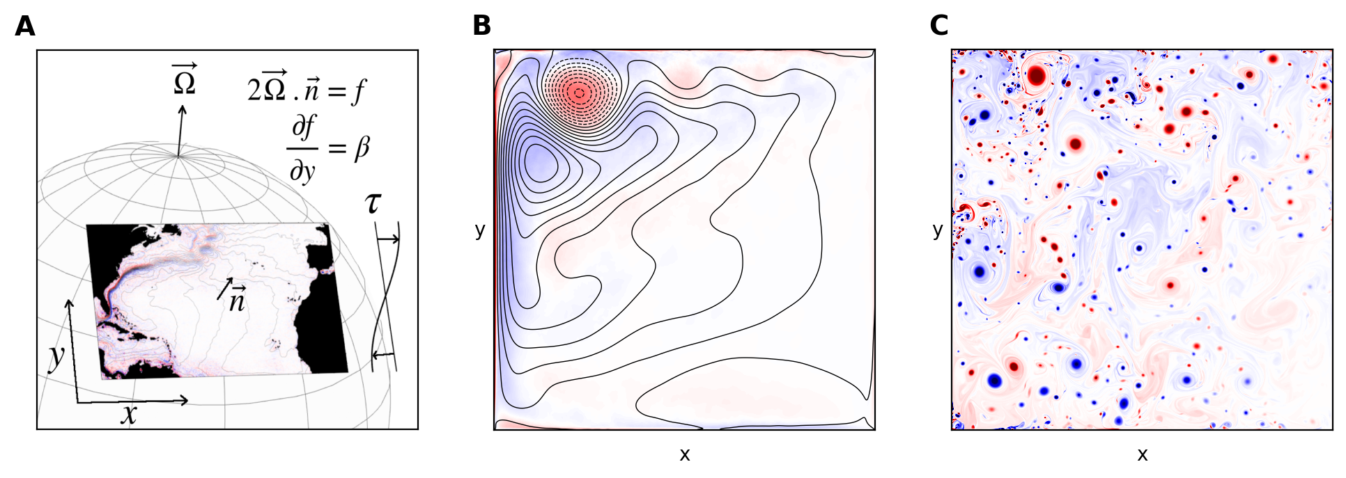
Figure 1: A: The beta-plane model with an inlet for the streamfunction of the time-average sea surface velocity field in the North Atlantic. Colors show the corresponding relative vorticity field. B: Temporal average of the streamfunction in the Gyre Turbulence regime ($\nu^{*}=2.5\times 10^{-5}$), superimposed on the corresponding relative vorticity field (colors) C: Snapshot of relative vorticity in the Gyre Turbulence regime ($\nu^{*}=2\times 10^{-6}$). Blue: anticyclonic vortices; red: cyclonic vortices.

Introduction. In three-dimensional turbulence, the transfer of energy from large to small scales results in an energy dissipation rate that remains independent of viscosity, regardless of its smallness Frisch (1995); Eyink and Sreenivasan (2006). This dissipative anomaly is a robust empirical observation sometimes referred to as the zeroth law of turbulence Dubrulle (2019). Conversely, two-dimensional flows are subject to an inverse energy cascade Boffetta and Ecke (2012), which results in the self-organization of the flow at the domain scale Bouchet and Venaille (2012). In order for dissipation to be efficient in two-dimensional flows, there needs to be an additional mechanism that creates small-scale structures where dissipation operates, thereby breaking the inverse cascade. The strong shear built up close to lateral boundaries could be a way to create such dissipative structures Deremble et al. (2016). In the context of Navier-Stokes equations, this possibility has been raised by simulations of a dipolar vortex interacting with a wall Farge et al. (2011). This study has sparked intense debate regarding the scaling of energy dissipation with viscosity in bounded two-dimensional turbulent flows Clercx and Van Heijst (2017); Waidmann et al. (2018); Sutherland et al. (2013). The existence of a dissipative anomaly in two-dimensional flows with boundaries would bear significant practical implications, for example in contributing to a deeper understanding of the energy cycle in the ocean Ferrari and Wunsch (2009); Zhai et al. (2010); Pearson and Fox-Kemper (2018). In fact, classical linear models for the emergence of western intensified currents Vallis (2017); Dalibard and Saint-Raymond (2018), such as the Gulf Stream or the Kuroshio, do provide a remarkable example of a dissipative anomaly. Here we show that this dissipative anomaly persists in a nonlinear regime, and unveil a new Gyre Turbulence regime with a western intensified mean flow and finite energy dissipation rate.

Flow model. The simplest model describing western intensification of oceanic currents is the rigid-lid barotropic quasigeostrophic model on a closed domain tangent to the Earth Vallis (2017):

$$\partial_{t}\omega+J(\psi,\omega)+\beta^{*} \partial_{x}\psi=\nu^{*}\Delta\omega-\partial_{y}\tau,$$ (1)

$$\omega=\Delta\psi,\quad \tau=-\cos\left(\pi y\right).$$ (2)

The term $J(\psi,\omega)=(u\partial_{x}+v\partial_{y})\ \omega$ is the advection of vorticity $\omega$ by the streamfunction $\psi$, with $u=-\partial_{y}\psi$ the zonal ($x$-direction) and $v=\partial_{x}\psi$ the meridional (y-direction) velocity components. We solve this two-dimensional model on a square domain. Forcing comes from the wind stress curl $-\partial_{y}\tau$. Time and length have been rescaled such that both the length of the domain $L$ and the maximum value of the wind stress $\tau_{0}$ are $1$. The shape of the forcing corresponds to a single gyre, and is somewhat relevant to the North Atlantic case, with net injection of negative vorticity, as observed in the subtropical gyre (figure 1A). The only difference to the incompressible two-dimensional Navier-Stokes equations is the beta term $\beta^{*}\partial_{x}\psi$. This term comes from the curl of the Coriolis force, assuming linear variations of the Coriolis parameter in the meridional direction $y$. This framework is called the beta plane approximation, and it captures the effects of differential rotation induced by a rotating planet Vallis (2017).

Importantly, we consider no-slip boundary conditions, with vanishing velocity at the boundary. Previous studies of the single gyre model assumed free-slip (or a mixture between free-slip and no-slip boundary conditions) and it has been found that lowering the viscosity led to an increasingly energetic mean flow Kamenkovich et al. (1995); Sheremet et al. (1995); Ierley and Sheremet (1995); Sheremet et al. (1997). The strong mean flow observed in these simulations did not have an intensified western boundary current and was hence regarded as irrelevant to the problem of oceanic circulation. At the same time, the organisation of the large-scale flow is thought to occur in an asymptotic regime in which molecular viscosity becomes unimportant. It was therefore argued that the flow model lacked essential physical features required to dissipate energy and evacuate vorticity Fox-Kemper and Pedlosky (2004); Berloff et al. (2002), that could for instance be parameterized by imposing enhanced dissipation in a region close to the boundary Fox-Kemper and Pedlosky (2004). We show below that using no-slip boundary conditions on all boundaries is sufficient to recover a highly turbulent regime with a western-intensified mean flow of finite energy.

Linear dynamics. Linear theories for wind-driven gyres compute steady states of equations (1)-(2), by neglecting the advection term Vallis (2017); Dalibard and Saint-Raymond (2018). In the domain bulk, the vorticity equation simplifies into Sverdrup balance, a cornerstone of midlatitude ocean dynamics: $\beta^{*}v=-\partial_{y}\tau$, meaning that an injection of negative vorticity is offset by a southward transport of the fluid. To ensure mass conservation, this interior circulation must be complemented by boundary layers. The majority of this recirculation occurs within the western boundary layer, thereby breaking the East-West symmetry established by the Sverdrup balance. In the viscous solution found by Munk (figure 2A, top left inlet) the boundary layer thickness scales as $\delta_{M}=(\nu^{*}/\beta^{*})^{1/3}$ Munk (1950), which implies that total dissipation is dominated by contributions from the boundary layer while energy injection comes from the domain bulk. The confinement of energy dissipation in a western boundary layer holds when viscosity is replaced by other dissipation mechanisms, such as a linear drag Vallis (2017). In general, large-scale gyre patterns and therefore energy injection do not depend on details of those linear boundary layers. This is a strong incentive to look for a turbulent dissipative anomaly in this system.

Nonlinear simulations. In order to explore the non-linear regimes we numerically solve the 2-dimensional model using Basilisk software (http://basilisk.fr, see supplementary material for details on the numerical scheme). The parameter space $(\nu^{*},\beta^{*})$ can then be dissected into four regions (figure 2A). In the limit of weak $\beta^{*}$, the effects of differential rotation are negligible with respect to other terms and the flow response is equivalent to that of the two-dimensional Navier-Stokes (NS) equations, with a transition from laminar to turbulent flow when $\nu^{*}$ decreases Clercx et al. (2005).

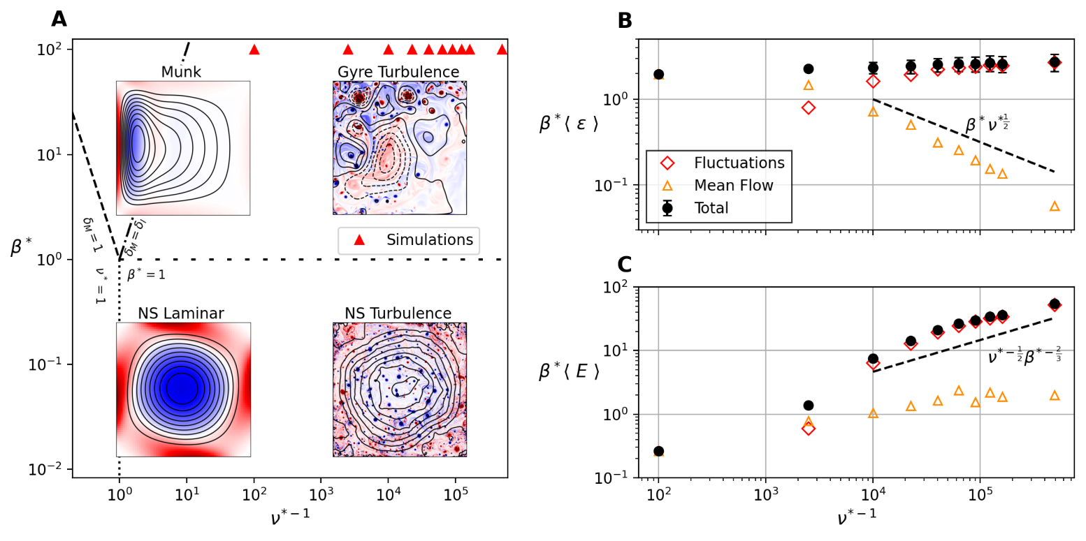
Figure 2: A: Parameter space (no-slip boundary conditions). Insets show typical instantaneous vorticity fields (color) and streamfunction (lines) B: Energy dissipation rate, rescaled by the energy injection through a Sverdrup interior. C: Energy rescaled by the energy of the inertial western boundary layer. Errorbars show the standard deviation.

If $\beta^{*}\gg 1$ then differential rotation becomes important. We expect that the Sverdrup balance will hold in the domain interior, and that a western intensified boundary layer will close the circulation. This western boundary layer is called inertial when nonlinear terms dominate over viscous terms. A Sverdrup scaling $U\sim\beta^{*-1}$ and a balance between nonlinear and beta term yields $\delta_{I}=\beta^{*-1}$ Charney (1955); Vallis (2017). The transition between this inertial regime and laminar Munk regime described earlier arise for $\delta_{M}=\delta_{I}$, i.e. $\nu^{*}=1/\beta^{*2}$. When viscosity is decreased below this threshold, the boundary layer becomes unstable, and those instabilities feed the domain with vortices. As viscosity is further decreased the system eventually enters into the Gyre Turbulence regime: while the time mean flow remains close to a Sverdrup interior with western intensified boundary layers (figure 1B), the instantaneous vorticity field is dominated by a vigorous heterogeneous vortex gas which is densest in the north-western corner of the domain (figure 1C). The gyre structure is not observed on instantaneous streamfunction fields, which is instead dominated by contributions arising from Rossby basin modes Pedlosky (2013) (not shown here), and to a lesser extent by contributions from the vortices. We now focus on the transition from the Munk solution to the Gyre Turbulence regime, using a set of simulations performed at $\beta^{*}=100$ with values of $\nu^{*}$ decreasing from $10^{-2}$ to $2\times 10^{-6}$.

Energy budget. Dissipation of the total energy $E=\int(u^{2}+v^{2})\ dA/2$ depends on the enstrophy $Z=\int\omega^{2}\ dA/2$ through the relation

$$\frac{\partial E}{\partial t}=\mathcal{P}-\varepsilon,\quad\mathcal{P}=\int\tau u\ dA,\quad\varepsilon=2\nu^{*}Z.$$ (3)

Time average and fluctuations are defined as

$$\langle\psi\rangle=\lim_{T\to\infty}\frac{1}{T}\int_{s}^{s+T}\psi\ dt,\quad\psi^{\prime}=\psi-\langle\psi\rangle,$$ (4)

where the integration is started from a moment $s$ in time after which the system is observed to be in statistical equilibrium, for which $\langle\mathcal{P}\rangle=\langle\varepsilon\rangle$.

The central result of this letter is depicted in figure 2B. In Gyre Turbulence, the average dissipation is observed to be insensitive to a decrease in $\nu^{*}$. Our rescaling by $\beta^{*-1}$ shows that the dissipation rate remains close to that predicted by energy injection through an interior flow governed by a Sverdrup balance. However, the dissipation mechanism changes drastically as the fluctuations become increasingly important at smaller values of $\nu^{*}$, while the mean flow contributes only a negligible fraction to the total dissipation. The importance of the fluctuations can also be seen in the total energy of the flow (figure 2C). The rescaling by $\beta^{*-1}$ reveals that the total energy of the mean flow remains close to the energy in a western inertial boundary layer, while the fluctuations become much stronger (for details on the proposed scaling see supplementary material).

Mean flow structure. In a statistically stationary flow, the time-averaged production term $\langle\mathcal{P}\rangle$ must also be independent of $\nu^{*}$, as it exactly balances the time-averaged dissipation $\langle\epsilon\rangle$. This constraint, together with the observation of figure 2B that the energy of the mean flow reaches a plateau, suggests that the bulk streamfunction $\langle\psi\rangle$ displayed in figure 1B only has a weak dependence on $\nu^{*}$ in the Gyre Turbulence regime. While the order of magnitude of the flow agrees with Sverdrup balance in the domain interior (figure 3A), the gyre pattern is different than the prediction from linear theory, likely due to nonlinear rectification mechanisms in the presence of Rossby waves Fox-Kemper (2004); Kramer et al. (2006). We observe only weak changes in this pattern when lowering viscosity in the Gyre Turbulence regime (see supplementary material).

The gyre pattern is connected to inertial boundary layers with a well defined functional relation between streamfunction and potential vorticity $\langle q\rangle=\langle\omega\rangle+\beta y$, such that $J(\langle q\rangle,\langle\psi\rangle)=0$. We identified two regions where such relations hold (figure 3), which we will call the inflow (blue) and the outflow (red) layer. The analysis of these layers will be carried out for the simulation at $\nu^{*}=2.5\times 10^{-5}$ as it out of the scope of our numerical resources to obtain smooth mean flows as lower values of $\nu^{*}$.

The inflow layer is consistent with classical theory predicting $\langle q\rangle=-(\beta^{*}/U_{in})\langle\psi\rangle$, which leads to a western boundary layer thickness $\delta_{I}=1/\beta^{*}$, where $U_{in}<0$ is the westward inflow, scaling as $1/\beta^{*}$ Charney (1955); Vallis (2017). The northward velocity in the inertial boundary layer is $U_{I}\sim 1$, so that mass transport in this layer compensates the Southward Sverdrup bulk transport. No-slip boundary condition is guaranteed by a Prandtl sublayer with thickness $\delta_{P}\sim\sqrt{\nu^{*}}$. The vorticity within this Prandtl layer is $\omega_{max}=U_{I}/\delta_{P}\sim 1/\sqrt{\nu^{*}}$. This scaling will play a central role to describe interior vortices.

The outflow layer close to the northern boundary has a negative $q-\psi$ relation that describes both a meandering jet with velocity $U_{out}$ and a strong cyclonic recirculation. Stationary Rossby wave meanders and a stationary vortex on a beta plane with mean flow $U_{out}$ both select the size $\sqrt{U_{out}/\beta^{*}}$. We assume that this length sets the vortex jet width denoted $\delta_{out}$, and that jet transport is set by the transport of the western boundary layer, which yields $\delta_{out}\sim\beta^{*-2/3}$ and $U_{out}\sim\beta^{*-1/3}$. An adaptation of classical Charney theory to this inertial region yields to $\langle q\rangle=-\beta^{*}/U_{out}\langle\psi\rangle+\beta^{*}$, which fits well with numerical results (see figure 3B and supplementary material).

The strong cyclonic recirculation that we observe in the mean flow is a signature of the presence of intense cyclonic vortices in this region (see figure 1C). These strong vortices result from the coalescence of smaller vortices in the interior. An increased vortex size leads to an increased vortex drift to the northwest, until a stationary state is reached. If merging continues, the vortex drifts to the northwest until interacting with the wall, which leads to its fragmentation. We observe that this fragmentation efficiently transfers energy from large to small scales, halting the inverse cascade and setting the largest turbulent scale in the system.

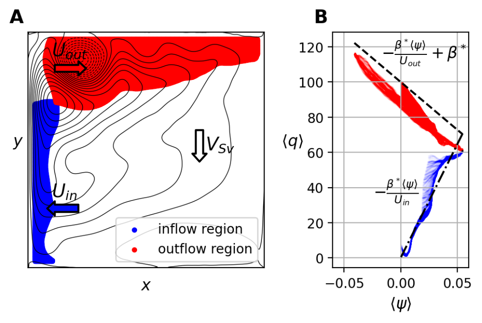
Figure 3: A: Contour plot of the mean stream function $\langle\psi\rangle$ at $\nu^{*}=2.5\times 10^{-5}$, with colored areas identified as inertial boundary layers. B: $q-\psi$ relations in the inertial boundary layers.

Statistics of dissipation. While the production term $\langle\mathcal{P}\rangle$ depends crucially on the mean flow, we showed that the dissipation term is dominated in the turbulent regime by contributions from fluctuations of vorticity (figure 2B). The dissipation is directly proportional to the values of $\omega^{2}$, of which we show the probability distribution function in figure 4A. The core of the distribution $\Pi(\log(\omega^{2}))$ is close to a Gaussian distribution, similar to recent observations from more comprehensive ocean models Pearson and Fox-Kemper (2018).

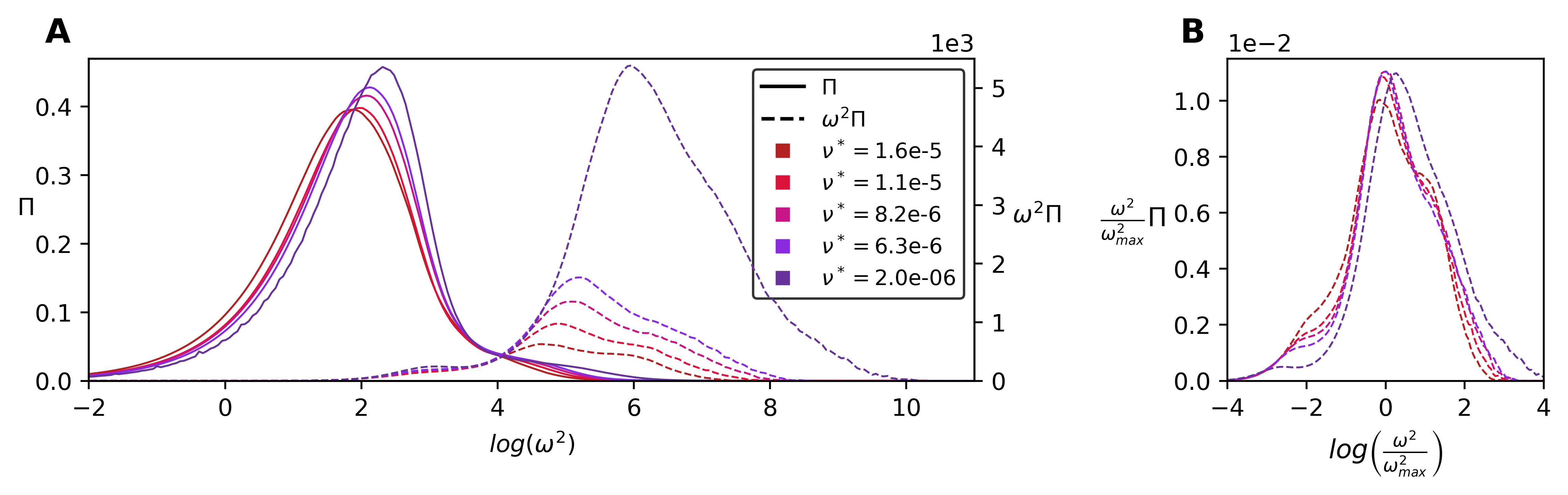
Figure 4: A: Probability Distribution functions $\Pi$ of $log(\omega^{2})$ for different values of $\nu^{*}$. Also shown are the values responsible for dissipation, $\omega^{2}\Pi$. B: Values responsible for dissipation after rescaling by $\omega_{max}$. The area under the curves is equal to the total dissipation $\langle\varepsilon\rangle$.

The peak of $\Pi(\log(\omega^{2}))$ changes little upon varying the viscosity, revealing that most of the values of vorticity in the bulk are only weakly dependent on $\nu^{*}$. A much stronger dependence on $\nu^{*}$ is observed in the tails of the distributions, where we notice important deviations from lognormality. In fact, the average dissipation is dominated by contributions from the tails, which can be seen by plotting the quantity $\omega^{2}\Pi$. We show these tails after rescaling the vorticity by $\omega_{max}$ (figure 4B), collapsing the tails onto a single curve centered around unity. This suggests that the primary mechanism for vorticity injection is the detachment of the Prandtl layer, and that total dissipation is dominated by intense vortices that result from the roll-up of the detached layer. Building upon this hypothesis and assuming that the detachment occurs over a length $\delta_{out}$ leads to vortices of typical size $\sqrt{\delta_{P}\delta_{out}}$. Using energy balance then leads to a total energy $E\sim\nu^{*-1/2}\beta^{*-5/3}$ (see supplementary material), which fits well with numerical results of figure 2B.

Discussion. We found a finite dissipation rate as the viscosity vanishes in a simple wind-driven ocean model, together with a mean flow pattern at the domain scale that remains western intensified. Although many pathways to dissipation act in the real ocean, our findings reveal that two-dimensional turbulence with no-slip boundary conditions is sufficient for the maintenance of Sverdrup-like gyres in a turbulent regime.

Small-scale vortices generated by boundary layer detachment coalesce in the domain bulk until they encounter the wall, which brings back energy from large to small scales. While such formation of small-scale vortices has previously been reported in two-dimensional flow model Clercx et al. (2005); Farge et al. (2011); Clercx and Van Heijst (2017), Gyre Turbulence provides an original example of an inviscid forced-dissipated 2D regime in which energy does not condense in a large-scale mean flow but is instead contained in small-scale fluctuations.

In periodic geometry, the spontaneous emergence of a vortex gas was first described during the early-stage evolution of a freely decaying small-scale random vorticity field McWilliams (1984). However, the longtime limit of this dynamics leads to a domain-scale dipolar vortex. A steady-state vortex gas can also be reached in stratified quasi-geostrophic flows forced by a baroclinically unstable mean flow and dissipated with bottom friction Arbic and Flierl (2004); Thompson and Young (2006); Venaille et al. (2011); Gallet and Ferrari (2020). More generally, adding a forcing term in the Navier-Stokes equations mimicking the effect of instabilities by amplifying vorticity extrema suppresses an inverse cascade and eventually yields a gas of small-scale vortices van Kan et al. (2022). In Gyre Turbulence, there is no such bulk instability, as the creation of intense vortex cores occurs only at the boundary layers.

While the large-scale flow pattern of Gyre Turbulence is consistent with inertial boundary layer theory at a qualitative level, a quantitative description of this pattern remains to be developed. For this, it will be necessary to describe the mixing of potential vorticity induced by the vortex gas. Assuming constant eddy viscosity provides useful insights Pedlosky (2013); Ierley and Ruehr (1986), but is energetically inconsistent and contradicts the heterogeneous vortex gas observed in our simulations. This calls for better parametrizations of vortex gases, as for instance proposed recently in the context of baroclinic turbulence Gallet and Ferrari (2020, 2021). More generally, it will be interesting to see whether the Gyre Turbulence regime controlled by boundary layer detachments persists in more complex ocean models.

Acknowledgements. This project has received financial support from the CNRS through the 80 Prime program, and was performed using HPC resources from GENCI-TGCC (Grant 2022-A0130112020). We warmly thank G. Roullet for insightfull inputs on this topic.

Supplementary material 1. Inertial boundary layers

In the theory of inertial inflow boundary layers the relation between $\psi$ and $q$ is established in an intermediate connection area just outside the boundary layer, where we expect the same functional relation between $\psi$ and $q$ to hold as inside the boundary layer (for details see Vallis (2017)). In the limit of vanishing boundary layer thickness, the dynamical balance in the boundary layer will be the advection of relative vorticity by the interior flow and the creation of relative vorticity by the beta-term. The thickness then scales like $\delta_{I}\sim\sqrt{-U_{in}/\beta^{*}}$, and the outer matching yields $q=-\beta^{*}\psi/U_{in}$.

In the simulations we identify two areas in which a functional relation between $q$ and $\psi$ holds. To identify these regions, we draw the isolines $u,v=0$ that cross the centre of the gyre (the maximum of $\langle\psi\rangle$ close to the western boundary). The inflow layer is defined as the area west of the line $v=0$ and south of $u=0$, whereas the outflow layer is defined as the area north of $u=0$ and east of $v=0$. We also cut out areas very close to the boundaries where we expect viscous effects to be dominant. The resulting areas are depicted in figure 3 in the main text.

For the outflow layer (with positive inflow velocity along the x-direction), a matching with domain interior is not self-consistent as the boundary layer thickness becomes imaginary and the solution becomes oscillatory. Furthermore, the inertial region does not reach the western part of the domain.

We noticed that this inertial region contains a meandering jet a cyclonic recirculation. Calling $\delta_{o}$ the jet width, calling $U_{out}$ the jet velocity, and assuming continuity of the mass transport between the western boundary layer and the meandering jet yields to

$$\delta_{o}U_{out}=U_{I}\delta_{I}=U_{Sv}L.$$ (5)

We observe that jet meanders wavelength and cyclonic recirculation radius are of the order of the jet width $\delta_{o}$. Meanders can be interpreted as a doppler-shifted Rossby wave, which is stationary when

$$\delta_{o}=\sqrt{U_{out}/\beta^{*}}.$$ (6)

This length also corresponds to the typical size of a statioary vortex on a beta plane in the presence of a mean flow $U_{out}$. Combining Eq. (6) and (5) yields to

$$\delta_{o}=\beta^{*-\frac{2}{3}},U_{out}=\beta^{*-\frac{1}{3}}.$$ (7)

To determine the functional relation between $\psi$ and $q$ in the outflow layer we consider the (non-inertial) region in the northwestern part of the domain. This region connect the western boundary layer in the inflow layer to the meandering jet of the outflow layer. Close to the outflow layer, we assume that the flow velocity is zonal with velocity $U_{out}>0$ and we neglect relative vorticity with respect to planerary vorticity (which is only marginally satisfied). In that case we can apply the same reasoning as classical inertial layer theory with $\langle q\rangle=\beta^{*}y$ and $\langle\psi\rangle=-U_{out}(y-L)$, assuming $\psi=0$ at the northern wall in the outflow layer. We hence retrieve the relation.

$$\langle q\rangle=-\beta^{*}/U_{out}\langle\psi\rangle+\beta^{*}L.$$ (8)

To test this relation, we diagnose the velocities $U_{in}$ and $U_{out}$ as the average zonal velocities along the isolines $v=0$ for each part of the gyres connected to the matching regions. This yields values of $U_{out}=0.18$ and $U_{in}=0.07$, for which the scaling theory gives the correct order of magnitude ($U_{out}\sim\beta^{*-\frac{1}{3}}=0.21$, $U_{in}\sim\beta^{*-1}=0.01$). Using the diagnosed values, the slopes given by inertial layer theory then agree well with the observed functional relations between $\langle\psi\rangle$ and $\langle q\rangle$ in both areas. The slight offset of the relation for the outflow may stem from the fact that the relative vorticity is not negligible in the matching region.

Supplementary material 2. Mean Flow Variations

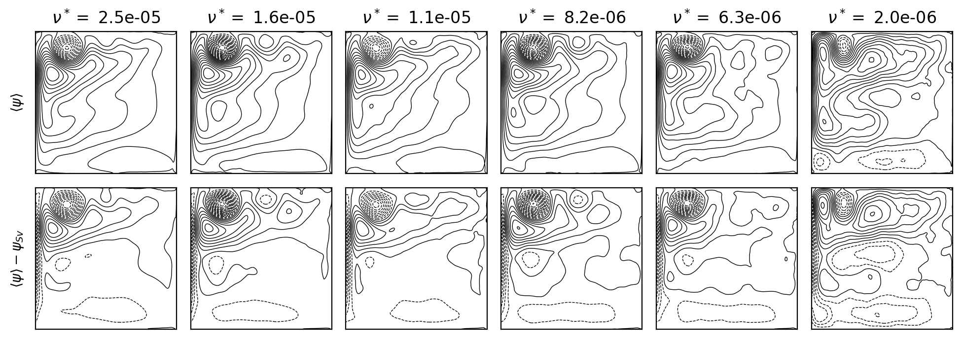
Figure 5: Top line: Mean stream function $\langle\psi\rangle$ for different values of $\nu^{*}$. Bottom line: Deviations from Sverdrup Flow. Contour lines are plotted with intervals $\beta^{*-1}$.

Although the energy of the mean flow remains constant its structure changes slightly when decreasing $\nu^{*}$ (figure 5). In the interior, the linear response of the system to the forcing gives the Sverdrup solution of the form

$$\psi_{Sv}=\frac{1}{\beta^{*}}\pi(1-x)\cos\left(\pi y\right)$$ (9)

If we subtract this from the mean stream function $\langle\psi\rangle$ we observe that the departures from this solution are mainly zonal structures and hence suggest that they results from the non-linear interaction of Rossby basin modes as in Fox-Kemper (2004) (also no inertial relation between $\langle\psi\rangle$ and $\langle q\rangle$ was observed in the interior).

Supplementary material 3. Scaling Analysis

In figure 2 of the main text we show that the dissipation of the mean flow decreases while the energy of the fluctuations increases. The aim of this section is to rationalize this observation. In the following, the sign $A\sim B$ means that there is a prefactor of order one between $A$ and $B$.

Let us start with the estimate of energy dissipation for the mean flow. It is assumed to be governed by the viscous sublayer that connects the inertial western boundary layer to the no-slip boundary condition Ierley and Ruehr (1986). Its thickness can be estimated as a Prandtl-like boundary layer:

$$\delta_{P}\sim\sqrt{\frac{\nu L}{U_{I}}}\sim\sqrt{\nu^{*}},$$ (10)

where $U_{I}\sim 1$ is the northward velocity in the inflow layer (in dimensional units $U_{I}\sim\sqrt{\tau_{0}L}$). The vorticity within the Prandtl-like layer then scales as

$$\omega_{max}\sim\frac{U_{I}}{\delta_{P}}\sim\frac{1}{\sqrt{\nu^{*}}}.$$ (11)

Assuming that total dissipation of the mean flow is dominated by contribution from this Prandtl-like layer then leads to

$$\varepsilon_{\text{mean flow}}\sim\nu\int\omega^{2}dA\sim\nu\omega_{max}^{2}\delta_{P}\sim\sqrt{\nu^{*}}.$$ (12)

This is consistent with the decay observed in figure 2B of the main text.

Let us now estimate the energy carried by fluctuations around the time averaged flow, which is much larger than the energy of the mean flow.

We assume that the flow is a vortex gas with $N$ vortices of core radius denoted $\lambda$ and vorticity value scaling as $\omega_{max}$. This scaling for the vorticity amounts to assuming that vortices are initially created through detachment of the viscous sublayer in the western inertial boundary layer, with a subsequent conservation of vorticity maxima during vortex coalescence.

We further assume that the boundary layer detachment occurs on a distance $\delta_{o}$ in the upper left corner of the domain (see main text). In that case the area of a detached vortex sheet scales like $\delta_{P}\delta_{o}$. Assuming that the boundary layer filament rapidly rolls up into a circular vortex preserving its area leads to

$$\lambda\sim\sqrt{\delta_{P}\delta_{o}}\sim\nu^{*1/4}{\beta^{*-1/3}}$$ (13)

This crude estimate only accounts for the production of negative vortices, but interaction of those vortices with the wall produce vortices with opposite circulation. We also implicitly neglect the merging between vortices (which must occur to create a vortex of size $\delta_{o}$ in the northern-western part of ocean).

The energy dissipation is estimated as the sum of the energy dissipation due to each of the vortices:

$$\varepsilon\sim\nu^{*}N\lambda^{2}\omega_{max}^{2}$$ (14)

This term is balanced by the production term $\mathcal{P}\sim\beta^{*-1}$. Using the Prandtl scaling for $\omega_{max}$ finally gives an estimate for the total area covered by the vortices:

$$N\lambda^{2}\sim\beta^{*-1}$$ (15)

We verify this estimate figure (6) by summing the area occupied by all values of vorticity larger than $\omega_{max}/10$ on a snapshot.

Finally, the energy of such a vortex gas scales like

$$E\sim N(\omega_{max}\lambda^{2})^{2}\sim\nu^{*-1/2}\beta^{*-5/3},$$ (16)

with additional logarithmic corrections Gallet and Ferrari (2020).

Albeit tentative, the proposed scaling incorprates several of the zeroth-order processes that we observe in the flow and yields a $\nu^{*}$-dependence of $E$ that agrees with observed values (figure 2 in main text).

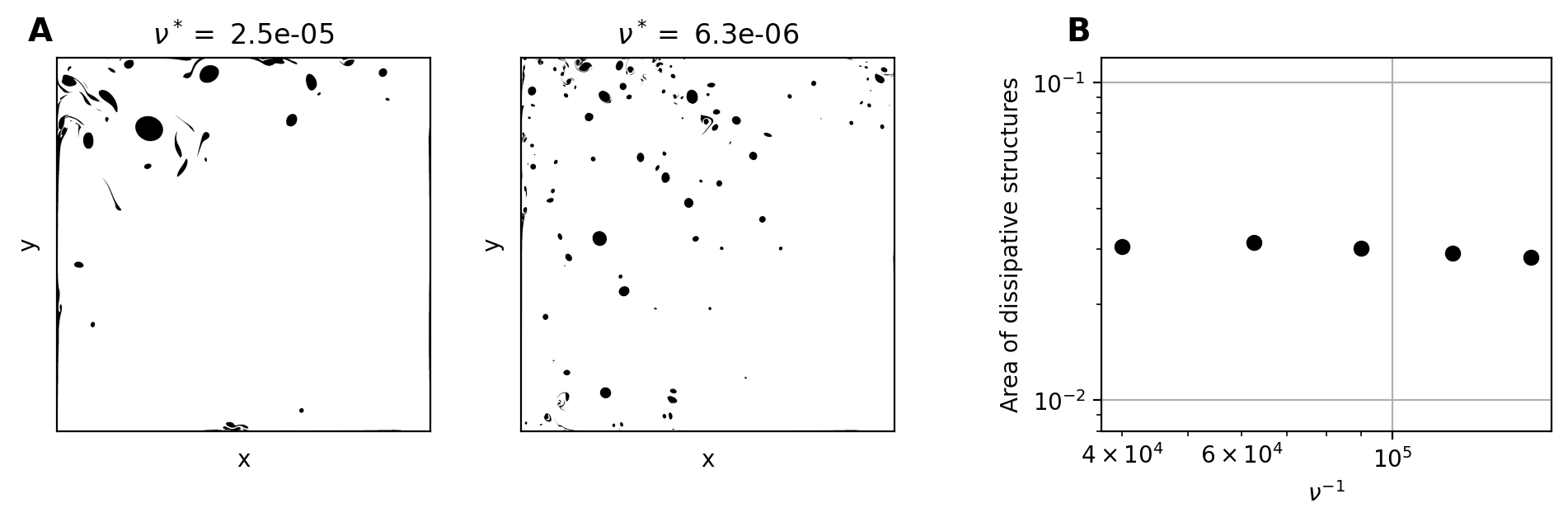
Figure 6: A: Snapshots of dissipative structures at two values of $\nu^{*}$. To create the binary images, we compare vorticity values to $\omega_{max}/10$. B Area of dissipative structures against $\nu^{*}$. Note how, although the structures become smaller (as shown in A), the total area remains constant (the prediction of area fraction from scaling analysis is $\beta^{*-1}=10^{-2}$).

Supplementary material 4. Numerical methods

For the numerical implementation of the quasigeostrophic equations we use the standard finite-difference discretization procedure. Vorticity and stream function are collocated at cell vertices and we use the Arakawa Jacobian for the advection term Cushman-Roisin and Beckers (2011). For the inversion of the elliptic equation (3), we use a multigrid method. Time integration is performed with a second order or corrector scheme. Impermeability conditions are achieved by imposing $\psi=0$ at the edges. The no-slip boundary condition is implemented by specifying the value of the vorticity on the sides for the viscous operator. By performing a Taylor expansion in the vicinity of the boundary (in this example, the western boundary) we get

$$\psi_{1}=\psi_{0}+\Delta\left.\frac{\partial\psi}{\partial x}\right|_{0}+\frac{\Delta^{2}}{2}\left.\frac{\partial^{2}\psi}{\partial x^{2}}\right|_{0}\,.$$ (17)

So at this order, the vorticity at the edge is

$$\omega_{0}=\left.\frac{\partial^{2}\psi}{\partial x^{2}}\right|_{0}=2\frac{\psi_{1}}{\Delta^{2}}\,,$$ (18)

since $\psi_{0}=0$ (no flow) and $\left.\partial\psi/\partial x\right|_{0}=0$ (no slip). In practice the methods outlined above work well in the domain interior, we therefore use them to timestep q in the interior. We then inverse $\omega$ to obtain psi, from which we can at last calculate the new values of $\omega$ at the boundaries with equation 18.

Almost all simulations that are discussed in the main text were performed at a numerical resolution of $2048\times 2048$ gridpoints. The only exception is the most turbulent run (at $\nu^{*}=2\times 10^{-6}$), which was performed at a resolution of $8192\times 8192$ gridpoints. To check for numerical convergence the simulation at $\nu^{*}=6.25\times 10^{-6}$ was relaunched with a doubled numerical resolution. Both its mean energy $\langle E\rangle$ and its mean dissipation $\langle\varepsilon\rangle$ changed by less than 5%.

References

- Frisch (1995) U. Frisch, Turbulence: the legacy of AN Kolmogorov (Cambridge university press, 1995).
- Eyink and Sreenivasan (2006) G. L. Eyink and K. R. Sreenivasan, Reviews of modern physics 78, 87 (2006).
- Dubrulle (2019) B. Dubrulle, Journal of Fluid Mechanics 867, P1 (2019).
- Boffetta and Ecke (2012) G. Boffetta and R. E. Ecke, Annual review of fluid mechanics 44, 427 (2012).
- Bouchet and Venaille (2012) F. Bouchet and A. Venaille, Physics reports 515, 227 (2012).
- Deremble et al. (2016) B. Deremble, W. Dewar, and E. Chassignet, J. Mar. Res 74, 249 (2016).
- Farge et al. (2011) M. Farge, K. Schneider, et al., Physical Review Letters 106, 184502 (2011).
- Clercx and Van Heijst (2017) H. Clercx and G. Van Heijst, Physics of Fluids 29, 111103 (2017).
- Waidmann et al. (2018) M. Waidmann, R. Klein, M. Farge, K. Schneider, et al., Journal of Fluid Mechanics 849, 676 (2018).
- Sutherland et al. (2013) D. Sutherland, C. Macaskill, and D. Dritschel, Physics of Fluids 25, 093104 (2013).
- Ferrari and Wunsch (2009) R. Ferrari and C. Wunsch, Annual Review of Fluid Mechanics 41, 253 (2009).
- Zhai et al. (2010) X. Zhai, H. L. Johnson, and D. P. Marshall, Nature Geoscience 3, 608 (2010).
- Pearson and Fox-Kemper (2018) B. Pearson and B. Fox-Kemper, Physical review letters 120, 094501 (2018).
- Vallis (2017) G. K. Vallis, Atmospheric and oceanic fluid dynamics (Cambridge University Press, 2017).
- Dalibard and Saint-Raymond (2018) A.-L. Dalibard and L. Saint-Raymond, Mathematical study of degenerate boundary layers: A large scale ocean circulation problem, Vol. 253 (American Mathematical Society, 2018).
- Kamenkovich et al. (1995) V. Kamenkovich, V. Sheremet, A. Pastushkov, and S. Belotserkovsky, Journal of marine research 53, 959 (1995).
- Sheremet et al. (1995) V. Sheremet, V. Kamenkovich, and A. Pastushkov, Journal of marine research 53, 995 (1995).
- Ierley and Sheremet (1995) G. R. Ierley and V. A. Sheremet, Journal of marine research 53, 703 (1995).
- Sheremet et al. (1997) V. Sheremet, G. Ierley, and V. Kamenkovich, Journal of marine research 55, 57 (1997).
- Fox-Kemper and Pedlosky (2004) B. Fox-Kemper and J. Pedlosky, Journal of Marine Research 62, 169 (2004).
- Berloff et al. (2002) P. S. Berloff, J. C. McWilliams, and A. Bracco, Journal of Physical Oceanography 32, 764 (2002).
- Munk (1950) W. H. Munk, Journal of Atmospheric Sciences 7, 80 (1950).
- Clercx et al. (2005) H. Clercx, G. Van Heijst, D. Molenaar, and M. Wells, Dynamics of atmospheres and oceans 40, 3 (2005).
- Charney (1955) J. G. Charney, Proceedings of the National Academy of Sciences 41, 731 (1955).
- Pedlosky (2013) J. Pedlosky, Geophysical fluid dynamics (Springer Science & Business Media, 2013).
- Fox-Kemper (2004) B. Fox-Kemper, Journal of Marine Research 62, 195 (2004).
- Kramer et al. (2006) W. Kramer, M. van Buren, H. Clercx, and G. van Heijst, Physics of Fluids 18, 026603 (2006).
- McWilliams (1984) J. C. McWilliams, Journal of Fluid Mechanics 146, 21 (1984).
- Arbic and Flierl (2004) B. K. Arbic and G. R. Flierl, Journal of Physical Oceanography 34, 2257 (2004).
- Thompson and Young (2006) A. F. Thompson and W. R. Young, Journal of physical oceanography 36, 720 (2006).
- Venaille et al. (2011) A. Venaille, G. K. Vallis, and K. S. Smith, Journal of Physical Oceanography 41, 1605 (2011).
- Gallet and Ferrari (2020) B. Gallet and R. Ferrari, Proceedings of the National Academy of Sciences 117, 4491 (2020).
- van Kan et al. (2022) A. van Kan, B. Favier, K. Julien, and E. Knobloch, Journal of Fluid Mechanics 952, R4 (2022).
- Ierley and Ruehr (1986) G. R. Ierley and O. G. Ruehr, Studies in Applied Mathematics 75, 1 (1986).
- Gallet and Ferrari (2021) B. Gallet and R. Ferrari, AGU Advances 2, e2020AV000362 (2021).
- Cushman-Roisin and Beckers (2011) B. Cushman-Roisin and J.-M. Beckers, Introduction to geophysical fluid dynamics: physical and numerical aspects (Academic press, 2011).