Simultaneous inference for monotone and smoothly time-varying functions under complex temporal dynamics

Abstract

We propose a new framework for the simultaneous inference of monotone and smoothly time-varying functions under complex temporal dynamics utilizing the monotone rearrangement and the nonparametric estimation. We capitalize the Gaussian approximation for the nonparametric monotone estimator and construct the asymptotically correct simultaneous confidence bands (SCBs) by carefully designed bootstrap methods. We investigate two general and practical scenarios. The first is the simultaneous inference of monotone smooth trends from moderately high-dimensional time series, and the proposed algorithm has been employed for the joint inference of temperature curves from multiple areas. Specifically, most existing methods are designed for a single monotone smooth trend. In such cases, our proposed SCB empirically exhibits the narrowest width among existing approaches while maintaining confidence levels, and has been used for testing several hypotheses tailored to global warming. The second scenario involves simultaneous inference of monotone and smoothly time-varying regression coefficients in time-varying coefficient linear models. The proposed algorithm has been utilized for testing the impact of sunshine duration on temperature which is believed to be increasing by the increasingly severe greenhouse effect. The validity of the proposed methods has been justified in theory as well as by extensive simulations.

Keywords: piecewise locally stationary, nonparametric, monotone rearrangement, bootstrap, moderately high dimension

1 Introduction

Estimating functions under monotone constraint is fundamental within the sphere of shape constraint problems, offering diverse applications in fields including global warming (e.g. Woodward & Gray (1993)), environmental investigation (e.g. Hussian et al. (2005)), biostatistics (e.g. Stylianou & Flournoy (2002)), and financial analysis (e.g. Aıt-Sahalia & Duarte (2003)). Over the past two decades, research on monotone regression has attracted increasing research interest, developing from traditional isotonic regression (e.g. Brunk (1969)), to refined smooth estimators (e.g. Mukerjee (1988); Mammen (1991); Dette et al. (2006)); and from univariate function as the above mentioned works to multivariate functions (e.g. Chatterjee et al. (2018); Deng et al. (2021)). Despite these advancements, most existing approach relies critically on the assumptions of independence or stationarity, which often falls short in long-span time series datasets as discussed in Dette & Wu (2022). Meanwhile, the smooth and increasing trends have been widely identified in climate change. A prominent example is Xu et al. (2018), which demonstrates via climate model that global temperature has a smooth and increasing trend. Xu et al. (2018) further warned an accelerated global warming according to this trend. In our real data analysis, we also identify the smooth and increasing trends as well as locally stationary patterns in temperature data, see Figure 1. This empirical evidence indicates that the new statistical tools for shape constraint analysis, especially the estimation of smooth and monotone regression functions are needed for investigating contemporary temporal-dependent real-world data.

(a) Monotone trend

(b) Nonstationarity

Figure 1: (a) The maximum temperature (°C) data in Heathrow with a fitted smooth time-varying trends, see Section 8; (b) Estimated autocorrelation functions by the method in Dette & Wu (2022) based on data in (a). The time-varying pattern implies the nonstationarity.

In this paper, we aim at the estimation and inference of the monotone and smoothly time-varying functions under complex temporal dynamics. In particular, we consider two very important scenarios where our methodology demonstrates its effectiveness. One is the estimation and jointly simultaneous inference of monotone trends from moderately high-dimensional nonstationary processes. This capability proves especially valuable when dealing with multiple time series that exhibit monotone behavior, such as temperature data collected from various weather stations within a geographic region. The other is the estimation and inference of the monotone time-varying coefficients, or more generally, monotone linear combination of time-varying coefficients in time-varying coefficient linear models. This enables us to assess the monotonically changing relationship between the response variable and predictor variables as time evolves. Such time-varying coefficient linear models with monotone condition could be useful in climate science, see for example Dhar & Wu (2023).

Our proposed SCB, which asymptotically centers around the the monotone estimator, is asymptotically correct. While some recent studies have considered dependent observation in the context of monotone regression (e.g. Anevski & Hössjer (2006), Zhao & Woodroofe (2012)), they primarily focus on pointwise limit distributions. Recently, Chernozhukov et al. (2009) and Bagchi et al. (2016) proposed methods for constructing SCBs for monotone signals, however, both their resulting SCBs are conservative. Bagchi et al. (2016) focuses on the inference under minimal smooth assumptions, hence their confidence band along with their estimates produces “jump” spots, which seems not optimal for the analysis of data sets with smoothly changing mechanisms. Moreover, except Chernozhukov et al. (2009), the above-mentioned literature and most current inference methods for monotone regression functions applicable to time series require the data to be strictly stationary. On the other hand, via improving an original SCB, Chernozhukov et al. (2009) produces monotone SCBs. However, those SCBs are not necessarily centered around the monotone estimator of the regression function.

In fact, inference for the entire monotone regression function is a fundamental and challenging problem in the literature which has attracted enormous endeavor. Besides the literature discussed in the last paragraph, the problem has been investigated under various specific settings and scenarios, including but not limited to the construction of SCBs in special monotone models (e.g. Sampson et al. (2009); Huang (2017); Gu et al. (2021)) or only over a finite grid in the domain with certain stochastic equicontinuity condition (e.g. Westling et al. (2020)). In contrast to the existing literature, our results significantly expand the application scope of inference methods for monotone regression functions to a broader range of real-world scenarios via allowing general time series nonstationarity as well as high-dimensional trend or multiple regression. We compare our methods with several mainstream methods for the statistical analysis of the monotone regression functions and summarize the corresponding results in Table 1.

Table 1: Comparison between our methodology and previous major study

Our methodology	Previous major work	Literature
Monotone rearrangement-based: - smooth function - produce strictly monotone estimator	Isotonic regression-based: - constrained optimization - almost inevitable flat point	Brunk (1969), Mukerjee (1988), Mammen (1991).
SCB under asymptotically correct significance level	Pointwise confidence interval or conservative SCB	Deng et al. (2021), Bagchi et al. (2016), Chernozhukov et al. (2009).
Nonstationary time series	Independent or stationary observation	Zhao & Woodroofe (2012), Bagchi et al. (2016).
- High-dimensional model i.e. $t\in[0,1]$, $p\rightarrow\infty$, $\mathbf{m}(t)\in\mathbb{R}^{p}$, is monotone in each coordinate. - Regression model i.e. $Y(t)=X^{\top}(t)\mathbf{m}(t)+e(t)$ $\mathbf{C}\mathbf{m}(t)\in\mathbb{R}^{s}$ is monotone for known $\mathbf{C}\in\mathbb{R}^{s\times p}$ in each coordinate.	Multivariate model i.e. $\mathbf{t}\in[0,1]^{p}$ but $m(\mathbf{t})\in\mathbb{R}$. The extension of our method adapting to this setting is left as a rewarding future work.	Chatterjee et al. (2018), Deng et al. (2021), Westling et al. (2020) .

Our simultaneous inference is based on monotone estimates for possibly high-dimensional monotone vector functions or for monotone regression coefficient functions, which combines the strength of nonparametric estimation and monotone rearrangement. Such estimator belongs to the class of two-step estimators that combines isotonization or rearrangement with smoothing. This class of estimators has been extensively discussed in the single trend with stationary noise setting; see, for example, Zhao & Woodroofe (2012), Bagchi et al. (2016). Our chosen rearranged estimates can be obtained by unconstrained optimization algorithm, which enables us to derive the corresponding stochastic expansion. We then apply the state-of-the-art Gaussian approximation technique in Mies & Steland (2023) to approximate the distribution of maximum deviation of the monotone estimates by certain Gaussian random variables or vectors. Upon this, we design two bootstrap algorithms to construct the (joint) SCBs for both scenarios of high-dimensional trends and time-varying coefficient linear models under smooth and monotone constraints. It is worth noting that our method is applicable to so-called piecewise locally stationary noise (see Zhou (2013) for details) which allows both smooth changes and abrupt changes in the underlying data-generating mechanisms. The validity of our proposed methods is justified theoretically, to which the key is controlling the approximation error via Nazarov’s inequality (Nazarov (2003)).

The remainder of this paper is structured as follows. In Section 3, we introduce the monotone rearrangement-based monotone estimator. Section 4 presents our main results for the high-dimensional model, including model assumptions, the theoretic results of Gaussian approximation, and the bootstrap procedure which mimics the limiting distribution of the maximum deviation of the monotone and smooth estimator. Similarly, the monotone and smooth estimation for time-varying coefficient linear model is discussed thoroughly in Section 5. In Section 6, we detail the selection scheme for tuning parameters. Furthermore, Section 7 reports our simulation results, while Section 8 presents the application of our method to the analysis of historical temperature data in the UK. Finally, in Section 9, we discuss potential directions for future work. Detailed proofs and additional simulation results can be found in the supplementary material. In particular, additional simulations compare the width of SCB obtained by our method with alternative SCBs and find that our SCB enjoys the narrowest width while maintaining confidence levels.

2 Notation

Before stating our results formally, we list the notations that will be used throughout the paper below. For a vector $\mathbf{v}=\left(v_{1},\cdots,v_{p}\right)^{\top}\in\mathbb{R}^{p}$, let $|\mathbf{v}|=(\sum_{j=1}^{p}v_{j}^{2})^{1/2}$. For a random vector $\mathbf{V}$, $q>0$, let $\|\mathbf{V}\|_{q}=\left(\mathbb{E}|\mathbf{V}|^{q}\right)^{1/q}$ denote the $\mathcal{L}^{q}$-norm of the random vector $\mathbf{V}$ and write $\mathbf{V}\in\mathcal{L}^{q}$ if $\left(\mathbb{E}|\mathbf{V}|^{q}\right)^{1/q}<\infty$. The notion $\|\cdot\|$ refers to $\|\cdot\|_{2}$ if no extra clarification. Denote $\mathrm{diag}\{a_{k}\}_{k=1}^{p}$ as a diagonal matrix with diagonal elements $a_{1},\dots,a_{p}$. Let $\lfloor x\rfloor$ represent the largest integer smaller or equal to $x$. For any two positive real sequences $a_{n}$ and $b_{n}$, write $a_{n}\asymp b_{n}$ if $\exists$ $0<c<C<\infty$ such that $c\leq\liminf_{n\rightarrow\infty}a_{n}/b_{n}\leq\limsup_{n\rightarrow\infty}a_{n}/b_{n}\leq C$. We use the notion $\hat{\mathbf{m}}^{\prime}(t)$ to represent the local linear estimator of derivative $\mathbf{m}^{\prime}(t)$ where $\mathbf{m}^{\prime}(t)=(\frac{\partial}{\partial t}m_{j}(t))_{1\leq j\leq p}$ for the sake of brevity.

3 Monotone estimator via monotone rearrangement

For simplicity, we start illustrating our methodology for univariate series in this section. Consider the classic nonparametric model with monotone constraint

$$Y(t)=m(t)+e(t),\quad t\in[0,1]$$ (3.1)

where $m(t)$ is a smoothly monotone function of $t$, and $e(t)$ is a zero-mean error process. In this paper, we allow $e(t)$ to be nonstationary, and all our results established are under a strictly increasing context. In other words, we focus on the mean function $m:[0,1]\rightarrow\mathbb{R}$ that is strictly increasing in $t$ for the sake of brevity. At each time point $t_{i}=:i/n$, we assume that only one realization $(y(t_{i}))$ is available, i.e., there is no repeated measurement. Further writing $y_{i}=Y(t_{i}),e_{i}=e(t_{i})$, the model (3.1) then can be written as

$$y_{i}=m(t_{i})+e_{i},\quad i=1,\dots,n.$$ (3.2)

For strictly decreasing cases our methods still apply via considering $\{-y_{i}\}_{i=1}^{n}$.

Numerous estimators have been derived for model (3.2) to obtain constrained estimators of $m(t)$ that satisfy the continuity and monotonicity constraint. A prevalent method for the inference of monotone shape functions is the fundamental isotonic regression, which yields a discontinuous “step” function with flat segments. To bridge the gap between step fitting and the continuous nature of the data, isotonization mixed with kernel smoothing procedure has been studied by a series of research, see for example Mammen (1991), Van Der Vaart & Van Der Laan (2003), Durot & Lopuhaä (2014). However, such approaches almost inevitably produce flat area in estimated curves even when the true function contains no flat part. Additionally, the spline-based methods, e.g. Ramsay (1988), Meyer (2008), can estimate a smooth and strictly increasing function. However, the above isotonization-based and spline-based methods rely on constrained optimization techniques. As a comparison, Dette et al. (2006) introduces a smooth and strictly monotone estimator via monotone rearrangement, which does not rest on constrained optimization. Therefore the statistical properties of estimator suggested by Dette et al. (2006) are easy to analyze. The monotone rearrangement techniques have been applied widely in solving statistical problems with monotone constraints, for example Chernozhukov et al. (2009), Chernozhukov et al. (2010), Dette & Volgushev (2008), Dhar & Wu (2023).

The key idea of monotone rearrangement is the use of the following fact. For any function $f$ defined on $[0,1]$, and a kernel density function $K_{d}(\cdot)$, define $g_{h_{d}}\circ f$ on $\mathbb{R}$ as

$$g_{h_{d}}\circ f:s\rightarrow\int_{0}^{1}\left\{\int_{-\infty}^{s}\frac{1}{h_{d}}K_{d}\left(\frac{f(x)-u}{h_{d}}\right)\mathrm{d}u\right\}\mathrm{d}x,$$

which is a smooth and monotone approximation of $f^{-1}$ when $f$ is strictly increasing; see Ryff (1970). Moreover, $g_{h_{d}}\circ f$ is always smooth and monotone, even if $f$ is non-monotone. Thus, a natural smooth and monotone estimator of $m^{-1}$ can be defined through Riemann sum approximation to $g_{h_{d}}\circ\hat{m}$, i.e.,

$$\hat{m}_{I}^{-1}(s)=:\int_{-\infty}^{s}\frac{1}{Nh_{d}}\sum_{i=1}^{N}K_{d}\left(\frac{\hat{m}(i/N)-u}{h_{d}}\right)\mathrm{d}u,$$ (3.3)

where $\hat{m}(\cdot)$ is a local linear estimator using kernel function $K_{r}(\cdot)$ and bandwidth $h_{r}$, i.e.

$$\left(\hat{m}(t),\hat{m}^{\prime}(t)\right)=:\underset{\eta_{0},\eta_{1}\in\mathbb{R}}{\arg\min}\left[\sum_{i=1}^{n}\left\{y_{i}-\eta_{0}-\eta_{1}\left(t_{i}-t\right)\right\}^{2}K_{r}\left(\frac{t_{i}-t}{h_{r}}\right)\right].$$ (3.4)

The construction of $\hat{m}_{I}^{-1}(s)$ is adopted from Dette et al. (2006), which primarily investigated pointwise asymptotic behavior based on independent observations. However, our research focus, which revolves around simultaneous inference, necessitates the examination of a time span rather than a single time point. Therefore, we introduce the index set $\hat{\mathcal{T}}$ on which all our simultaneous results are built:

$$\hat{\mathcal{T}}=:\left\{\hat{m}_{I}^{-1}(s):s\in\hat{\mathcal{T}}^{-1}\right\}\cap[h_{d}\log h_{d}^{-1},1-h_{d}\log h_{d}^{-1}],$$ (3.5)

where $\hat{\mathcal{T}}^{-1}=:\{s\in\mathbb{R}:\min_{1\leq i\leq N}\hat{m}(i/N)\leq s\leq\max_{1\leq i\leq N}\hat{m}(i/N)\}$. The interval $\hat{\mathcal{T}}$ enjoys several advantageous properties. First, on the set $\hat{\mathcal{T}}^{-1}$, $\hat{m}_{I}^{-1}(s)$ is smooth and strictly monotone, which enables us to naturally derive a smooth monotone estimator $\hat{m}_{I}(t)$ for $m(t),t\in\hat{\mathcal{T}}$ by directly inverting $\hat{m}_{I}^{-1}(s)$. Second, this interval circumvents boundary issues that arise in monotone rearrangement using the kernel density function $K_{d}(\cdot)$. Despite $\hat{\mathcal{T}}$ being a proper subset of $[0,1]$, it is sufficiently large for simultaneous inference since the length of $[0,1]$ not covered by $\hat{\mathcal{T}}$ converges to zero in probability, as supported by the Proposition A.1 in supplement.

In the following Section 4 and Section 5, we further consider the high-dimensional version and time-varying regression extension of the monotone estimator $\hat{m}_{I}(t)$ and the corresponding simultaneous inference methods. The simultaneous inference of $m(t)$ for (3.1) in this section could be performed via the methods in Section 4 and Section 5 since $m(t)$ is a special case of signals considered in Sections 4 and 5, and will not be discussed separately for the sake of brevity.

4 Joint SCBs for high-dimensional monotone trends

In the past decades, the increasing need to study contemporary time series with rapidly growing size and progressively complex structure has necessitated the construction of SCBs that cover many time-varying curves jointly, which is essential for the simultaneous inference in numerous applications involving processes that are $p$-dimensional. A prominent example is the investigation of global warming trends across multiple districts. While in each district the temperature recorded may exhibit variations, they commonly adhere to the monotonicity condition. Constructing joint SCBs that simultaneously cover all the monotone temperature trends in those districts at a desired significance level can be useful for comprehensively understanding the extreme climate change on a global scale. This motivates us to consider the high-dimensional extension of model (3.2) with the following form: for $i=1,\dots,n$; $k=1,\dots,p$

$$y_{i,k}=m_{k}(t_{i})+e_{i,k}$$ (4.1)

where $\mathbf{y}_{i}=(y_{i,1},\dots,y_{i,p})^{\top}=(y_{1}(t_{i}),\dots,y_{p}(t_{i}))^{\top}$ is our observed $p$-dimensional process and $\mathbf{e}_{i}=(e_{i,1},\dots,e_{i,p})^{\top}$ is a high-dimensional nonstationary error process. Moreover, each coordinate of the mean vector function $\mathbf{m}(t)=(m_{1}(t),\dots,m_{p}(t))^{\top}$ is assumed to be monotone, i.e., $m_{k}(x)\leq m_{k}(y)$ if $x\leq y$ for all $k=1,\dots,p$. It is worth pointing out that our monotonicity is different from multivariate monotone regression model, e.g. Deng et al. (2021), which considers a $\mathbb{R}$ valued function $m(\mathbf{t})$ on $p$-dimensional index set $\mathbf{t}\in[0,1]^{p}$. In the remaining of the section, we discuss assumptions on the time series in Subsection 4.1, the Gaussian approximation in Subsection 4.2 and the Algorithm of generating joint SCBs in Subsection 4.3.

4.1 Assumptions of high-dimensional time series

To begin with, we impose the following assumptions on the high-dimensional trends:

(A1)

For the vector function $\mathbf{m}(t)=(m_{1}(t),\dots,m_{p}(t))^{\top}$ where $t\in[0,1]$, the second derivative $m_{k}^{\prime\prime}(t)$ of the function $m_{k}(t)$ exists and is Lipschitz continuous on $[0,1]$. The Lipschitz constants are bounded for all $k=1,\dots,p$.

(A2)

For the vector function $\mathbf{m}(t)=(m_{1}(t),\dots,m_{p}(t))^{\top}$, there exists a universal constant $M>0$ s.t. $\inf_{t\in[0,1]}m_{k}^{\prime}(t)\geq M$, $\forall k=1,\dots,p$.

In fact, we assume $t\in[0,1]$ for simplicity. For general scenario $t\in\mathcal{I}$ for some interval $\mathcal{I}$, our method still works by simple modification. Let $\varepsilon_{i}$, $i\in\mathbb{Z}$ be i.i.d. random elements and $\mathcal{F}_{i}=(\dots,\varepsilon_{i-1},\varepsilon_{i}).$ We assume that the high-dimensional nonstationary error $\mathbf{e}_{i}$ is generated by following causal representation:

$$\mathbf{e}_{i}=\mathbf{G}_{i}(\mathcal{F}_{i}),\quad i=1,\dots,n$$

where $\mathbf{G}_{i}=(G_{i,1},\dots,G_{i,p})^{\top}$ is a measurable vector function. We further introduce the physical dependence measure of Wu (2005) for $p$-dimensional $\mathbf{G}_{i}(\mathcal{F}_{i})$.

Definition 4.1.

(physical dependence measure) Let $\{\varepsilon_{i}^{\prime}\}_{i\in\mathbb{Z}}$ be an i.i.d. copy of $\{\varepsilon_{i}\}_{i\in\mathbb{Z}}$. For $i\geq k$, Let $\mathcal{F}_{i,k}=(\dots,\varepsilon_{k-1},\varepsilon_{k}^{\prime},\varepsilon_{k+1},\dots,\varepsilon_{i})$. Define the physical dependence measure for the stochastic system $\mathbf{G}_{i}\left(\mathcal{F}_{i}\right)$ as

$$\delta_{q}(\mathbf{G},k)=\sup_{1\leq i\leq n}\left\{\left\|\mathbf{G}_{i}\left(\mathcal{F}_{i}\right)-\mathbf{G}_{i}\left(\mathcal{F}_{i,i-k}\right)\right\|_{q}\right\}.$$ (4.2)

The physical dependence measure we defined in (4.2) shows an input-output-based dependence measure quantifying the influence of the input $\varepsilon_{i-k}$ on the output $\mathbf{G}_{i}(\mathcal{F}_{i})$, which is different from the classic mixing conditions. Alternative definitions of dependence measure for high-dimensional time series can be found, for example in Zhang & Cheng (2018), where the dependence measure is specified to each dimension i.e. $\delta_{q}(G_{j},k),j=1,\dots,p$ and requires a universal summation decay i.e. $\sum_{k=l}^{\infty}\sup_{1\leq j\leq p}\delta_{q}(G_{j},k)<\infty$. Our assumptions on dependence measure is related to their framework in the sense that $\sum_{k=l}^{\infty}\delta_{q}(\mathbf{G},k)\leq\sqrt{p}\sum_{l=k}^{\infty}\sup_{1\leq j\leq p}\delta_{q}(G_{j},k)$. Furthermore, we define the long-run covariance matrix function for the nonstationary process $\mathbf{e}_{i}=\mathbf{G}_{i}(\mathcal{F}_{i})$.

Definition 4.2.

For the nonstationary process $\mathbf{G}_{i}(\mathcal{F}_{i})$, define the long-run covariance matrix function

$$\mathbf{\Sigma}_{\mathbf{G}}(i)=:\sum_{l\in\mathbb{Z}}\mathrm{cov}(\mathbf{G}_{i}(\mathcal{F}_{0}),\mathbf{G}_{i}(\mathcal{F}_{l})).$$ (4.3)

The long-run covariance matrix is important for quantifying the stochastic variation of the sums of the nonstationary process. We now introduce the assumptions on physical dependence measure, long-run covariance and other properties of the considered high-dimensional nonstationary process $\mathbf{G}_{i}(\mathcal{F}_{i})$:

(B1)

For some $q\geq 2$ and $\alpha\in(0,1)$, $\delta_{q}(\mathbf{G},k)\leq\Theta(p)\chi^{k}$ with $p=O(n^{\alpha}),\Theta(p)=O(n^{\alpha})$.

(B2)

$\sup_{1\leq i\leq n}\|\mathbf{G}_{i}(\mathcal{F}_{0})\|_{q}\leq\Theta(p)$, for some $q\geq 2$.

(B3)

$\sum_{i=2}^{n}\|\mathbf{G}_{i}(\mathcal{F}_{0})-\mathbf{G}_{i-1}(\mathcal{F}_{0})\|\leq\Theta(p)$.

(B4)

There exists constant $\Lambda\geq\underline{\Lambda}>0$ such that all the eigenvalues of long-run covariance matrix $\mathbf{\Sigma}_{\mathbf{G}}(i)$ are bounded between $\underline{\Lambda}$ and $\Lambda$ for any $i=1,\dots,n$.

(B5)

For any $e_{i,k}$, $i=1,\dots,n$, $k=1,\dots,p$, there exists a universal constant $t>0$ such that $\mathbb{E}(\exp(t|e_{i,k}|))\leq C<\infty$.

Remark 4.1.

$\Theta(p)$ reflects the dimension factor for both physical dependence measure and the moment conditions of the $p$-dimensional process. If $\delta_{q}(G_{j},k)\leq C\chi^{k}$ for all $j=1,\dots,p$ with constant $C>0$, then $\Theta(p)$ would be a rate of $\sqrt{p}$. Further suppose that all $p$ components are independent, then (B5) implies that $\Theta(p)$ in (B2) will also be a rate of $\sqrt{p}$.

Assumptions (B1), (B2), and (B4) are in line with many kernel-based nonparametric analysis of nonstationary time series such as Zhao (2015) and Dette & Wu (2022). While this paper adopts a geometric decay in (B1), it is worth noting that a polynomial decay can yield similar results. However, this requires more complicated conditions and substantially more intricate mathematical arguments. Therefore, for simplicity, we stick to the geometric decay assumption. Assumption (B3) can be regarded as an extension of the locally stationary assumption. For example, it encompasses scenarios akin to the piecewise locally stationary concept, as discussed in Zhou (2013), where the time series can experience abrupt changes at several breakpoints over time, rendering it a more flexible and realistic representation for various practical applications. Assumption (B5) allows sub-exponential tails, and is mild for high-dimensional models. It can be relaxed to allow polynomial tails if the dimension $p$ is fixed. For a more detailed illustration, we verify these assumptions by a general class of high-dimensional error process in Example B.1 at supplement.

4.2 Monotone estimation and Gaussian approximation

To estimate the monotone high-dimensional trend $\mathbf{m}(t)$, we apply monotone rearrangement on each dimension. The monotone estimator is written as $\hat{\mathbf{m}}_{I}(t)=(\hat{m}_{I,1}(t),\dots,\hat{m}_{I,p}(t))^{\top}$ where $\hat{m}_{I,k}(t)$ is the inverse of

$$\hat{m}_{I,k}^{-1}(s)=:\int_{-\infty}^{s}\frac{1}{Nh_{d,k}}\sum_{i=1}^{N}K_{d}\left(\frac{\tilde{m}_{k}(i/N)-u}{h_{d,k}}\right)\mathrm{d}u.$$ (4.4)

The $\tilde{m}_{k}(t)=2\hat{m}_{k,h_{r,k}/\sqrt{2}}(t)-\hat{m}_{k,h_{r,k}}(t)$ is the jackknife bias-corrected local linear estimator which has a bias of O($h_{r,k}^{3}$) towards the $k_{th}$ component of $\mathbf{m}(t)$, where

$$\left(\hat{m}_{k,h_{r,k}}(t),\hat{m}_{k,h_{r,k}}^{\prime}(t)\right)=:\underset{\eta_{0},\eta_{1}\in\mathbb{R}}{\arg\min}\left[\sum_{i=1}^{n}\left\{y_{i,k}-\eta_{0}-\eta_{1}\left(t_{i}-t\right)\right\}^{2}K_{r}\left(\frac{t_{i}-t}{h_{r,k}}\right)\right].$$ (4.5)

Before stating our main results, we make several assumptions and simplification on our kernel methods. Suppose there exists $h_{r},h_{d}$ s.t. $\min_{1\leq k\leq p}h_{r,k}\asymp h_{r}\asymp\max_{1\leq k\leq p}h_{r,k}$ and $\min_{1\leq k\leq p}h_{d,k}\asymp h_{d}\asymp\max_{1\leq k\leq p}h_{d,k}$. Then we assume:

(C1)

The kernel functions $K_{d},K_{r}$ are symmetric kernel density with compact support $[-1,1]$ and bounded second order derivatives.

(C2)

$n=O(N),nh_{r}^{3}\rightarrow\infty,nh_{r}^{7}\rightarrow 0,h_{d}=o(h_{r}),Nh_{d}^{3}\rightarrow\infty$, $R_{n}/h_{d}=o(1)$ where $R_{n}=h_{r}^{2}+\log^{3}n/\sqrt{nh_{r}}$.

Remark 4.2.

We use the Epanechnikov kernel for both $K_{d}$ and $K_{r}$ throughout the simulation and data analysis. Other kernels satisfying (C1) work similarly. Our assumption $R_{n}/h_{d}=o(1)$ is also weaker than the condition $R_{n}^{2}/h_{d}^{3}=o(1)$ in Dette et al. (2006)

Define the time span $\hat{\mathcal{T}}=\cap_{k=1}^{p}\hat{\mathcal{T}}_{k}$ where $\hat{\mathcal{T}}_{k}$ is defined in the same way as (3.5) with $\hat{m}_{k}(t)$ so that $\hat{m}_{I,k}(t)$ is well defined for each $k=1,\dots,p$. To construct joint SCBs for $\hat{\mathbf{m}}_{I}(t)-\mathbf{m}(t)$ on the time span $\hat{\mathcal{T}}$, the key result is to learn the maximum deviation i.e. $\max_{1\leq k\leq p}\sup_{t\in\hat{\mathcal{T}}}|\hat{m}_{I,k}(t)-m_{k}(t)|$. The following proposition provides the Gaussian approximation of this maximum deviation and serves as the basis for our simultaneous inference and further bootstrap procedure.

Proposition 4.1.

Suppose (A1),(A2),(B1)-(B5) and (C1)-(C2) are satisfied. Then there exists independent $\mathbf{V}_{j}=(V_{j,1},\dots,V_{j,p})^{\top}\sim N_{p}(0,\mathbf{\Sigma}_{\mathbf{G}}(j)),j=1,\dots,n$,on a richer probability space s.t.

$$\max_{1\leq k\leq p}\sup_{t\in\hat{\mathcal{T}}}\left|\sqrt{nh_{r}}(m_{k}(t)-\hat{m}_{I,k}(t))-\sqrt{nh_{r}}\mathcal{V}_{k}(t)\right|=O_{p}\left\{\frac{R_{n}^{2}\sqrt{nh_{r}}}{h_{d}}+\frac{\Theta(p)\sqrt{n\log n}\left(\frac{p}{n}\right)^{\frac{q-2}{6q-4}}}{\sqrt{nh_{r}}}\right\},$$ (4.6)

where the $p$-dimensional Gassuian vector process $\mathcal{V}(t)=(\mathcal{V}_{1}(t),\dots,\mathcal{V}_{p}(t))^{\top}$ with

$$\mathcal{V}_{k}(t)=\frac{m_{k}^{\prime}(t)}{Nh_{d,k}nh_{r,k}}\sum_{j=1}^{n}\sum_{i=1}^{N}K_{d}\left(\frac{m_{k}(i/N)-m_{k}(t)}{h_{d,k}}\right)\tilde{K}_{r}^{*}\left(\frac{j/n-i/N}{h_{r,k}},\frac{i}{N}\right)V_{j,k},$$

$$\tilde{K}_{r}^{*}\left(\frac{j/n-t}{h_{r,k}},t\right)=\frac{\nu_{2,k}(t)\tilde{K}_{r}\left(\frac{j/n-t}{h_{r,k}}\right)-\nu_{1,k}(t)\tilde{K}_{r}\left(\frac{j/n-t}{h_{r,k}}\right)\left(\frac{j/n-t}{h_{r,k}}\right)}{\nu_{0,k}(t)\nu_{2,k}(t)-\nu_{1,k}^{2}(t)},$$ (4.7)

$$\nu_{l,k}(t)=\int_{-t/h_{r,k}}^{(1-t)/h_{r,k}}x^{l}K_{r}(x)\mathrm{d}x$$ (4.8)

and $\tilde{K}_{r}(x)$ is jackknife kernel $\tilde{K}_{r}(x)=:2\sqrt{2}K_{r}\left(\sqrt{2}x\right)-K_{r}\left(x\right)$.

Remark 4.3.

$\sqrt{nh_{r}}\mathcal{V}(t)$ is a valid nondegenerate Gaussian process in the sense that there exists a constant $\underline{\sigma}>0$ such that $\min_{1\leq k\leq p}\operatorname{Var}(\sqrt{nh_{r}}\mathcal{V}_{k}(t))\geq\underline{\sigma}^{2}$, which has be shown in the proof of Theorem 4.1. The rate in the right side of (4.6) can be $o_{p}(1)$ if divergent $p=O(nh_{r}^{3})^{1/4-\alpha}$ for some $\alpha\in(0,1/4)$ with typical scaling $\Theta(p)\asymp\sqrt{p}$, sufficiently large $q$, and appropriate $h_{d}$.

4.3 Bootstrap algorithm of joint SCBs

Following Proposition 4.1, we can investigate $\max_{1\leq k\leq p}\sup_{t\in\hat{\mathcal{T}}}\sqrt{nh_{r}}|m_{k}(t)-\hat{m}_{I,k}(t)|$ through studying $\max_{1\leq k\leq p}\sup_{t\in\hat{\mathcal{T}}}|\sqrt{nh_{r}}\mathcal{V}_{k}(t)|$. However, it is sophisticated to study the limiting distribution of $\max_{1\leq k\leq p}\sup_{t\in\hat{\mathcal{T}}}|\sqrt{nh_{r}}\mathcal{V}_{k}(t)|$ due to the high dimensionality and the complicated time-varying covariance structure of $\mathcal{V}_{k}(t)$. One direct approach is to generate copies of the estimated $\mathcal{V}_{k}(t)$ and obtain empirical quantiles of their maxima, where the estimated $\mathcal{V}_{k}(t)$ is a Gaussian random variable having the form analogous to $\mathcal{V}_{k}(t)$, with the unknown quantities $m_{k}(t)$, $m_{k}^{\prime}(t)$, and $\mathbf{\Sigma}_{\mathbf{G}}(j)$ replaced by appropriate estimators. However, it is widely recognized that accurately estimating $m_{k}^{\prime}(t)$ can be challenging. Moreover, the estimation of $\mathbf{\Sigma}_{\mathbf{G}}(j)$ can also be difficult if $\mathbf{G}_{i}(\mathcal{F}_{i})$ is piecewise locally stationary since the breakpoints are difficult to identify, yielding inconsistency around the abrupt changes of the long run covariance for usual nonparametric estimators as seen in works such as Zhou (2013), Zhang & Wu (2015), Bai & Wu (2023b).

  Algorithm 1 Bootstrap for joint SCBs of $\mathbf{m}(t)$

 

Data: $\mathbf{y}_{i}\in\mathbb{R}^{p},i=1,\dots,n$

Initialization: Choose bandwidths $h_{r,k}$, $h_{d,k}$ and the window size $L$ by Section 6.  

Step 1: Obtain the jackknife estimator $\tilde{m}_{k}(t)=2\hat{m}_{k,h_{r,k}/\sqrt{2}}(t)-\hat{m}_{k,h_{r,k}}(t)$ with $\hat{m}_{k,h_{r,k}}(t)$ defined in (4.5).

Step 2: Obtain the monotone estimator $\hat{\mathbf{m}}_{I}(t)$ defined above (4.4).

Step 3: Obtain the residual $\hat{\boldsymbol{\varepsilon}}(t_{i})=(\hat{\varepsilon}_{1}(t_{i}),\dots,\hat{\varepsilon}_{p}(t_{i}))^{\top}$ where $\hat{\varepsilon}_{k}(t_{i})=y_{i,k}-\tilde{m}_{k}(t_{i})$ and derive the estimated cumulative long-run covariance $\hat{\mathbf{Q}}(j)$ defined in (4.10).

Step 4: Given data, generate $\mathbf{V}_{j}^{*}|\mathcal{F}_{n}\sim N_{p}(0,\hat{\mathbf{Q}}(j)-\hat{\mathbf{Q}}(j-1))$, $j=1,\dots,n$, where $V_{j}^{*}s$ are independent of each other conditional on the data, and calculate

$$\mathcal{V}^{*}(t)=:\sum_{j=1}^{n}\sum_{i=1}^{N}\mathcal{W}(i/N,t)\mathcal{K}_{r}(j/n,i/N)\mathbf{V}_{j}^{*},$$ (4.9)

where $\mathcal{W}(i/N,t)=\mathrm{diag}\left\{\hat{W}_{i,k,I}^{*}(t)\right\}_{k=1}^{p}$, $\hat{W}_{i,k,I}^{*}(t)=\hat{W}_{i,k,I}(t)/\sum_{i=1}^{N}\hat{W}_{i,k,I}(t)$ and

$$\hat{W}_{i,k,I}(t)=K_{d}\left(\frac{\tilde{m}_{k}(i/N)-\hat{m}_{I,k}(t)}{h_{d,k}}\right),\quad\mathcal{K}_{r}(j/n,i/N)=\mathrm{diag}\left\{\frac{1}{nh_{r,k}}\tilde{K}^{*}_{r}\left(\frac{j/n-i/N}{h_{r,k}},\frac{i}{N}\right)\right\}_{k=1}^{p}.$$

Step 5: Repeat step 4 for $B$ times and obtain the sample $\Big{\{}\max_{1\leq k\leq p}\sup_{t\in\hat{\mathcal{T}}}\Big{|}\mathcal{V}^{*(r)}_{k}(t)\Big{|}\Big{\}}_{r=1,...B}$. Let $\hat{q}_{1-\alpha}$ be the $(1-\alpha)_{th}$ sample quantile.

Output: Level $(1-\alpha)$ joint SCBs $\hat{\mathbf{m}}_{I}(t)\pm\hat{q}_{1-\alpha}\mathcal{B}_{p}$, where $\mathcal{B}_{p}=\{\mathbf{u}\in\mathbb{R}^{p}:|\mathbf{u}|\leq 1\}$ is the unit ball.

 

To overcome the above two difficulties we consider the bootstraping $\mathcal{V}^{*}(t)$ in (4.9) of Algorithm 4.3, whose formula (4.9) does not involve $m_{k}^{\prime}(t)$. Moreover, recent progress in Gaussian approximation (Mies & Steland (2023)) shows that the consistency of the cumulative long-run covariance estimator, instead of the uniform consistency of the time-varying long-run covariance estimator, is sufficient for the jointly simultaneous inference. In this paper, we estimate $\mathbf{Q}(k)=:\sum_{i=1}^{k}\boldsymbol{\Sigma}_{\mathbf{G}}(i)$ by

$$\hat{\mathbf{Q}}(k)=\sum_{i=L}^{k}\frac{1}{L}\left(\sum_{j=i-L+1}^{i}\hat{\boldsymbol{\varepsilon}}(t_{j})\right)\left(\sum_{j=i-L+1}^{i}\hat{\boldsymbol{\varepsilon}}(t_{j})\right)^{\top},$$ (4.10)

where $\hat{\boldsymbol{\varepsilon}}(t_{i})=(\hat{\varepsilon}_{1}(t_{i}),\dots,\hat{\varepsilon}_{p}(t_{i}))^{\top}$ are the nonparametric residuals, i.e. $\hat{\varepsilon}_{k}(t_{i})=y_{i,k}-\tilde{m}_{k}(t_{i})$. A similar estimator for the cumulative long-run covariance has been studied by Mies & Steland (2023), where the original series, instead of the residuals, is used since Mies & Steland (2023) assumes the data has zero mean when estimating $\mathbf{Q}(k)$. In the online supplement, we show that the estimation error for cumulative long-run covariance ${\mathbf{Q}}(k)$ using $\hat{\mathbf{Q}}(k)$ is relatively small w.r.t ${\mathbf{Q}}(k)$ by Lemma A.3. With the use of $\hat{\mathbf{Q}}(t)$ in Algorithm 4.3, we introduce the following theorem which shows that the distribution of our bootstrap samples given data uniformly approximates the distribution of $\max_{1\leq k\leq p}\sup_{t\in\hat{\mathcal{T}}}\left|\mathcal{V}_{k}(t)\right|$.

Theorem 4.1.

Recall the Gaussian process $\mathcal{V}(t)$ defined in Proposition 4.1. Suppose

$$\frac{\log(Np)\log^{2}(n)(\sqrt{np\varphi_{n}}+\varphi_{n}+p)}{nh_{r}}=o(1),$$ (4.11)

where $\varphi_{n}=:\Theta^{2}(p)(\sqrt{npL}+nL^{-1})+p^{3/2}L\sqrt{n}\left(\Theta(p)R_{n}+\sqrt{n}h_{r}^{5}+\sqrt{n}\log^{6}(n)/(nh_{r})\right)$. Assuming the conditions in Proposition 4.1 hold and

$$\frac{\Theta(p)\left(\frac{p}{n}\right)^{\frac{q-2}{6q-4}}\sqrt{n\log(Np)}\log n}{\sqrt{nh_{r}}}=o(1),\quad \frac{\sqrt{nh_{r}\log(Np)\log(np)}}{Nh_{d}}=o(1),$$ (4.12)

then (4.6) holds and we have

$$\sup_{x\in\mathbb{R}}\left|\mathbb{P}\left\{\max_{1\leq k\leq p}\sup_{t\in\hat{\mathcal{T}}}\left|\mathcal{V}_{k}(t)\right|\leq x\right\}-\mathbb{P}\left\{\max_{1\leq k\leq p}\sup_{t\in\hat{\mathcal{T}}}\left|\mathcal{V}^{*}_{k}(t)\right|\leq x\,\middle|\,\mathcal{F}_{n}\right\}\right|\rightarrow_{p}0,$$

where $\mathcal{V}^{*}(t)=(\mathcal{V}^{*}_{1}(t),\dots,\mathcal{V}^{*}_{1}(t))^{\top}$ is our bootstrap Gaussian process defined in (4.9).

Together with Gaussian approximations in Proposition 4.1, we justify the validity of our bootstrap algorithm for the construction of joint SCBs. We have the following remark for the rate conditions.

Remark 4.4.

Under the typical scaling $\Theta(p)\asymp\sqrt{p}$, both (4.11) and (4.12) can be satisfied with $nh_{r}^{6}\rightarrow\infty$, $\lfloor L\rfloor\asymp(n/p)^{1/3}$, $p\asymp(nh_{r}^{6})^{1/7-\alpha}$ for a sufficiently small $\alpha>0$, if $q$ and $N$ are sufficiently large. Simulation results in Section 7 reveal that our method works well with $p$ diverging at a rate faster than $(nh_{r}^{6})^{1/7-\alpha}$. We leave the refinement on the theory to allow faster diverging rate of $p$ using sharper inequalities as a rewarding future work.

5 Time-varying coefficient linear regression

Besides monotone trends, monotonicity also arises in time-varying relationships between variables. For example, greenhouse gases such as carbon dioxide, methane, and water vapor, can help to regulate Earth’s temperature by trapping heat from the sun that would otherwise be radiated back into space, creating so called natural greenhouse effect; see Anderson et al. (2016) for details. However, since the Industrial Revolution, human activities have substantially elevated the concentrations of greenhouse gases. As a result, even with the same duration of sunlight, we can experience a more significant temperature rise in more recent time due to the reason that a portion of the heat, which would have been radiated back to space in earlier times, is now trapped by these gases; see Kweku et al. (2018) for details. Based on this we can identify that there exists a smoothly increasing relationship between the response variable (temperature) and the predictor (sunshine duration).This motivates us to consider the following time-varying coefficient linear model

$$y_{i}=\mathbf{x}_{i}^{\top}\mathbf{m}(t_{i})+e_{i}$$ (5.1)

where $y_{i}=Y(t_{i}),\mathbf{x}_{i}=X(t_{i}),e_{i}=e(t_{i})$ represent the response (e.g. temperature), $p$-dimensional covariate process (e.g. sunshine duration, rain falls, etc.), and the zero-mean error process, respectively, while $\mathbf{m}(t)=(m_{1}(t),\dots,m_{p}(t))^{\top}$ denotes the $p$-dimensional time-varying coefficients. In this section, we consider model (5.1) with fixed dimension $p$; the scenario of diverging $p$ is much more complicated and will be left as a rewarding future work. To reflect the increasing relationship, in model (5.1) we further assume the following monotonicity constraint: there exists a known $\mathbf{C}\in\mathbb{R}^{s\times p}$ s.t. each coordinate function of the $\mathbf{m}_{\mathbf{C}}(t)=:\mathbf{C}\mathbf{m}(t)$ is smoothly increasing. For example, consider (8.2) in the data analysis where the choice of $\mathbf{C}=(0,1)$ reflects a smoothly increasing relationship between sunshine duration and temperature. Our inference is based on the jackknife bias-corrected local linear estimator for model (5.1) defined as $\tilde{\mathbf{m}}(t)=2\hat{\mathbf{m}}_{h_{r}/\sqrt{2}}(t)-\hat{\mathbf{m}}_{h_{r}}(t)$ where

$$\left(\hat{\mathbf{m}}_{h_{r}}(t),\hat{\mathbf{m}}^{\prime}_{h_{r}}(t)\right)=:\underset{\eta_{0},\eta_{1}\in\mathbb{R}^{p}}{\arg\min}\left[\sum_{i=1}^{n}\left\{y_{i}-\mathbf{x}_{i}^{\top}\eta_{0}-\mathbf{x}_{i}^{\top}\eta_{1}\left(t_{i}-t\right)\right\}^{2}K_{r}\left(\frac{t_{i}-t}{h_{r}}\right)\right].$$ (5.2)

Similar to (3.3), we define our monotone estimator through monotone rearrangement i.e.

$$\hat{m}_{\mathbf{C},I,k}^{-1}(v)=\int_{-\infty}^{v}\frac{1}{Nh_{d}}\sum_{i=1}^{N}K_{d}\left(\frac{\tilde{m}_{\mathbf{C},k}(i/N)-u}{h_{d}}\right)\mathrm{d}u$$ (5.3)

where $\tilde{m}_{\mathbf{C},k}(t)$ is the $k_{th}$ coordinate of $\tilde{\mathbf{m}}_{\mathbf{C}}(t)=:\mathbf{C}\tilde{\mathbf{m}}(t)$. Define $\hat{\mathbf{m}}_{\mathbf{C},I}(t)=:(\hat{m}_{\mathbf{C},I,1}(t),\dots,\hat{m}_{\mathbf{C},I,s}(t))^{\top}$ where $\hat{m}_{\mathbf{C},I,k}(t)$ is the inverse of $\hat{m}_{\mathbf{C},I,k}^{-1}(v)$ defined in (5.3), and consequently $\hat{\mathbf{m}}_{\mathbf{C},I}(t)$ serves as our monotone estimator of ${\mathbf{m}}_{\mathbf{C}}(t)$. We consider $(\mathbf{x}_{i})$ and $(e_{i})$ generated from

$$\mathbf{x}_{i}=\mathbf{H}_{i}(\mathcal{F}_{i})\quad\text{and}\quad e_{i}=G_{i}(\mathcal{F}_{i}),\quad i=1,\dots,n,$$

where $\mathbf{H}_{i}=:(H_{i,1},\dots,H_{i,p})^{\top}$ and $G_{i}$ are measurable functions. The quantities $H_{i,1},i=1,\dots,n,$ are fixed to be $1$, representing the intercept of the regression coefficients. Furthermore, we make the following assumptions on both $(\mathbf{x}_{i})$ and $(e_{i})$:

(B1’)

There exists a Lipschitz continuous matrix function $\mathbf{M}(t)$ s.t. $\mathbf{M}(t_{i})=:\mathbb{E}\left\{\mathbf{H}_{i}\left(\mathcal{F}_{0}\right)\mathbf{H}_{i}\left(\mathcal{F}_{0}\right)^{\top}\right\}$ and the smallest eigenvalue of $\mathbf{M}(t)$ is bounded away from zero for all $t\in[0,1]$.

(B2’)

$\sup_{1\leq i\leq n}\left\{\left\|\mathbf{H}_{i}\left(\mathcal{F}_{0}\right)\right\|_{4}\right\}<\infty$ and $\|\mathbf{H}_{i}\left(\mathcal{F}_{0}\right)-\mathbf{H}_{j}\left(\mathcal{F}_{0}\right)\|\leq L|i-j|/n,\forall 1\leq i,j\leq n$ for some constant $L>0$.

(B3’)

For $\mathbf{U}_{i}\left(\mathcal{F}_{i}\right)=:\mathbf{H}_{i}\left(\mathcal{F}_{i}\right)G_{i}\left(\mathcal{F}_{i}\right)$, $\sum_{i=2}^{n}\|\mathbf{U}_{i}(\mathcal{F}_{0})-\mathbf{U}_{i-1}(\mathcal{F}_{0})\|<\infty$.

(B4’)

$\delta_{4}(\mathbf{U},k)=O(\chi^{k})$ for some $\chi\in(0,1)$ and $\sup_{1\leq i\leq n}\left\{\left\|\mathbf{U}_{i}\left(\mathcal{F}_{0}\right)\right\|_{4}\right\}<\infty$

(B5’)

The smallest eigenvalue of the long-run covariance matrix function $\mathbf{\Lambda}(i)=:\mathbf{\Sigma}_{\mathbf{U}}(i)$ is bounded away from 0 for all $i=1,\dots,n$.

Assumptions (B1’) and (B2’) are standard in the literature of analysing time-varying coefficient linear models and have also been used in Zhou & Wu (2010). Assumptions (B3’)-(B5’) coincide with (B1)-(B4) with fixed dimension, allowing the error process $(e_{i})$ to be piecewise locally stationary. Notice that (B2’) requires $(\mathbf{x}_{i})$ to be locally stationary, since if $(\mathbf{x}_{i})$ is piecewise locally stationary the local linear estimator (5.2) is no longer consistent. With the above assumptions, the following Theorem 5.1 presents Gaussian approximation of the maximum deviation $\max_{1\leq k\leq s}\sup_{t\in\hat{\mathcal{T}}}|\hat{m}_{\mathbf{C},I,k}(t)-m_{\mathbf{C},k}(t)|$ and provides a valid bootstrap method for mimicking the behavior of the Gaussian process which approximates the maximum deviation.

Theorem 5.1.

Let conditions (B1’)-(B5’), (C1)-(C2) hold and the $\mathbb{R}^{s}$-valued function $\mathbf{m}_{\mathbf{C}}(t)$ satisfy conditions (A1)-(A2). Recall $\tilde{K}_{r}^{*}$ defined in (4.7), we have following two results:
(i). There exists independent Gaussian random vector $\mathbf{V}_{j}=:(V_{j,1},\dots,V_{j,s})^{\top}\sim N_{s}(0,\mathbf{\Sigma}_{\mathbf{C}}(j))$, $j=1,\dots,n$ such that

$$\max_{1\leq k\leq s}\sup_{t\in\hat{\mathcal{T}}}\left|\sqrt{nh_{r}}(\hat{m}_{\mathbf{C},I,k}(t)-m_{\mathbf{C},k}(t))-\sqrt{nh_{r}}\mathcal{V}_{\mathbf{C},k}(t)\right|=O_{p}(\rho_{n}\sqrt{nh_{r}}),$$ (5.4)

where $\rho_{n}=:R_{n}^{2}/h_{d}+n^{1/4}\log^{2}(n)/(nh_{r})$, $\mathbf{\Sigma}_{\mathbf{C}}(j)=:\mathbf{C}\mathbf{M}^{-1}(t_{j})\mathbf{\Lambda}(j)\mathbf{M}^{-1}(t_{j})\mathbf{C}^{\top}$ and

$$\mathcal{V}_{\mathbf{C},k}(t)=:\frac{m_{\mathbf{C},k}^{\prime}(t)}{Nh_{d}}\sum_{i=1}^{N}K_{d}\left(\frac{m_{\mathbf{C},k}(i/N)-m_{\mathbf{C},k}(t)}{h_{d}}\right)\frac{1}{nh_{r}}\sum_{j=1}^{n}\tilde{K}_{r}^{*}\left(\frac{j/n-i/N}{h_{r}},\frac{i}{N}\right)V_{j,k}.$$

(ii). Suppose $\hat{\mathbf{\Sigma}}_{\mathbf{C}}(j)=:\mathbf{C}\hat{\mathbf{M}}^{-1}(t_{j})\hat{\mathbf{\Lambda}}(j)\hat{\mathbf{M}}^{-1}(t_{j})\mathbf{C}^{\top}$ where

$$\hat{\mathbf{M}}(t_{j})=:\frac{1}{nh_{r}}\sum_{i=1}^{n}\mathbf{x}_{i}\mathbf{x}_{i}^{\top}\{(t_{i}-t_{j}^{*})/h_{r}\}^{l}K_{r}\left(\frac{t_{i}-t_{j}^{*}}{h_{r}}\right)$$

with $t_{j}^{*}=\max\{h_{r},\min(t_{j},1-h_{r})\}$ and

$$\hat{\mathbf{\Lambda}}(j)=:\frac{1}{L}\left(\sum_{i=j-L+1}^{j}\mathbf{x}_{i}\hat{\varepsilon}(t_{i})\right)\left(\sum_{i=j-L+1}^{j}\mathbf{x}_{i}\hat{\varepsilon}(t_{i})\right)^{\top},\quad\hat{\varepsilon}(t_{i})=:y_{i}-\mathbf{x}_{i}^{\top}\tilde{\mathbf{m}}(t_{i}).$$ (5.5)

Let $\bar{\varphi}_{n}=:\sqrt{nL}+nL^{-1}+\sqrt{n}L\left(h_{r}^{2}+\log(n)/\sqrt{nh_{r}}\right)+nL\left(h_{r}^{5}+\log^{2}n/(nh_{r})\right)$. If

$$\frac{\log(N)\log^{2}(n)(\sqrt{n\bar{\varphi}_{n}}+\bar{\varphi}_{n})}{nh_{r}}=o(1),\quad\sqrt{nh_{r}\log(N)\log(n)}=o(Nh_{d}),$$

and $\rho_{n}\sqrt{nh_{r}}=o(1)$, then there exists random vectors $\mathbf{V}_{j}^{*}=:(V_{j,1}^{*},\dots,V_{j,s}^{*})^{\top},j=1,\dots,n,$ which are conditionally independent given data and follow $\mathbf{V}_{j}^{*}|\mathcal{F}_{n}\sim N_{s}(0,\hat{\mathbf{\Sigma}}_{\mathbf{C}}(j))$ such that

$$\sup_{x\in\mathbb{R}}\left|\mathbb{P}\left\{\max_{1\leq k\leq s}\sup_{t\in\hat{\mathcal{T}}}\left|\mathcal{V}_{\mathbf{C},k}(t)\right|\leq x\right\}-\mathbb{P}\left\{\max_{1\leq k\leq s}\sup_{t\in\hat{\mathcal{T}}}\left|\mathcal{V}^{*}_{\mathbf{C},k}(t)\right|\leq x\,\middle|\,\mathcal{F}_{n}\right\}\right|\rightarrow_{p}0,$$ (5.6)

where

$$\mathcal{V}_{\mathbf{C},k}^{*}(t)=:\frac{1}{nh_{r}}\sum_{j=1}^{n}\sum_{i=1}^{N}\hat{W}_{i,k,I}^{*}(t)\tilde{K}_{r}^{*}\left(\frac{j/n-i/N}{h_{r}},\frac{i}{N}\right)V_{j,k}^{*},$$ (5.7)

$$\hat{W}_{i,k,I}(t)=K_{d}\left(\frac{\tilde{m}_{C,k}(i/N)-\hat{m}_{C,I,k}(t)}{h_{d}}\right),\quad\hat{W}_{i,k,I}^{*}(t)=\hat{W}_{i,k,I}(t)/\sum_{i=1}^{N}\hat{W}_{i,k,I}(t).$$

Result (i) provides the Gaussian approximation towards the maximum deviation but leaves challenges in estimating $\mathbf{m}_{\mathbf{C}}^{\prime}(t)$ and the long-run covariance related quantity $\mathbf{\Sigma}_{\mathbf{C}}(j)$. Result (ii) avoids estimating $\mathbf{m}_{\mathbf{C}}^{\prime}(t)$ and provides an appropriate estimator $\hat{\mathbf{\Sigma}}_{\mathbf{C}}(j)$ for $\mathbf{\Sigma}_{\mathbf{C}}(j)$ with negligible cumulative errors. Combining (i) and (ii) in Theorem 5.1, we propose Algorithm 5 for constructing the joint SCBs of $\mathbf{m}_{\mathbf{C}}(t)$ in practice, of which the validity is guaranteed by Theorem 5.1.

  Algorithm 2 Bootstrap for joint SCBs of $\mathbf{m}_{\mathbf{C}}(t)$

 

Data: $(y_{i},\mathbf{x}_{i})$, $i=1,\dots,n$ and known matrix $\mathbf{C}\in\mathbb{R}^{s\times p}$.

Initialization: Choose bandwidth $h_{r}$, $h_{d}$ and window size $L$ by Section 6.  

Step 1: Obtain the estimator $\tilde{\mathbf{m}}_{\mathbf{C}}(t)=2\hat{\mathbf{m}}_{h_{r}/\sqrt{2}}(t)-\hat{\mathbf{m}}_{h_{r}}(t)$ with $\hat{\mathbf{m}}_{h_{r}}(t)$ defined in (5.2).

Step 2: Obtain the monotone estimator $\hat{\mathbf{m}}_{\mathbf{C},I}(t)$ defined below (5.3).

Step 3: Calculate $\hat{\mathbf{\Sigma}}_{\mathbf{C}}(j)=\mathbf{C}\hat{\mathbf{M}}^{-1}(t_{j})\hat{\mathbf{\Lambda}}(j)\hat{\mathbf{M}}^{-1}(t_{j})\mathbf{C}^{\top}$ by plugging in

$$\hat{\mathbf{M}}(t_{j})=:\frac{1}{nh_{r}}\sum_{i=1}^{n}\mathbf{x}_{i}\mathbf{x}_{i}^{\top}\{(t_{i}-t_{j}^{*})/h_{r}\}^{l}K_{r}(\frac{t_{i}-t_{j}^{*}}{h_{r}}),\quad t_{j}^{*}=\max\{h_{r},\min(t_{j},1-h_{r})\},$$

and $\hat{\mathbf{\Lambda}}(j)$ in (5.5) with window size $L$.

Step 4: Given data, generate the Gaussian vector process $\mathcal{V}^{*}_{\mathbf{C}}(t)=:(\mathcal{V}^{*}_{\mathbf{C},1}(t),\dots,\mathcal{V}^{*}_{\mathbf{C},s}(t))^{\top}$ where $\mathcal{V}_{\mathbf{C},k}^{*}(t)$ is defined in (5.7).

Step 5: Repeat step 4 for $B$ times and obtain the samples $\Big{\{}\max_{1\leq k\leq s}\sup_{t\in\hat{\mathcal{T}}}\Big{|}\mathcal{V}^{*(r)}_{\mathbf{C},k}(t)\Big{|}\Big{\}}_{1\leq r\leq B}$. Let $\hat{q}_{1-\alpha}$ be the $(1-\alpha)_{th}$ sample quantile.

Output: Level $(1-\alpha)$ joint SCBs $\hat{\mathbf{m}}_{\mathbf{C},I}(t)\pm\hat{q}_{1-\alpha}\mathcal{B}_{s}$ where $\mathcal{B}_{s}=\{\mathbf{u}\in\mathbb{R}^{s}:|\mathbf{u}|\leq 1\}$.

 

6 Tuning parameter selection

To implement our method one needs to select bandwidths $h_{r}$, $h_{d}$ and window size $L$ in (3.4), (3.3) and (4.3) respectively. The first bandwidth $h_{r}$ is introduced to apply local linear estimation, which we select via the General Cross Validation (GCV) selector proposed by Craven & Wahba (1978). This method has been applied in various fields of nonstationary time series regressions (see for example Wu & Zhou (2017); Bai & Wu (2023a)) and also works well in our simulation and data analysis. To be precise, for each dimension $k$ in model (4.1), we can write $\hat{\mathbf{Y}}_{k}=\mathbf{Q}(h_{k})\mathbf{Y}_{k}$ for some square matrix $\mathbf{Q}$, where $\mathbf{Y}_{k}=(y_{1,k},\dots,y_{n,k})^{\top}$ and $\hat{\mathbf{Y}}_{k}=(\hat{y}_{1,k},\dots,\hat{y}_{n,k})^{\top}$ denote the vector of observed values and estimated values respectively, and $h_{k}$ is the bandwidth. Then we choose the bandwidth as $\hat{h}_{r,k}$ where

$$\hat{h}_{r,k}=\underset{h_{k}}{\arg\min}\{\operatorname{GCV}(h_{k})\},\quad\operatorname{GCV}(h_{k})=\frac{n^{-1}|\mathbf{Y}_{k}-\hat{\mathbf{Y}}_{k}|^{2}}{[1-\operatorname{tr}\{\mathbf{Q}(h_{k})\}/n]^{2}}.$$

We can apply above procedure to each dimension and then select an average bandwidth $\hat{h}_{r}=\sum_{k=1}^{p}\hat{h}_{r,k}/p$ for high-dimensional model. The GCV for model (5.1) follows the same formula with $\mathbf{Y}=(y_{1},...,y_{n})^{\top}$ and $\hat{\mathbf{Y}}=(\hat{y}_{1},...,\hat{y}_{n})^{\top}$.

The second bandwidth $h_{d}$ is introduced for the monotone rearrangement based on the local linear estimates, which in practice is usually chosen to be small as long as the assumption (C2) on $h_{r}$ and $h_{d}$ is satisfied. Following Dette et al. (2006), choosing $h_{d}$ that is much smaller than $h_{r}$ can mitigate bias caused by monotone rearrangement and boundary effects (see also Dette & Wu (2019)) while the analysis results are also insensitive to $h_{d}$ as long as it is small. In our simulation and data analysis practice, we recommend $h_{d}=h_{r}^{3}$ which also coincides with numerical results in Dette et al. (2006).

As for window size $L$ in (4.10), we recommend the minimum volatility (MV) method advocated by Politis et al. (1999). Let $\hat{\mathbf{Q}}(k)^{(L)}$ denote the quantity $\hat{\mathbf{Q}}(k)$ in (4.10) using window size $L$, then the MV method suggests that the estimator $\hat{\mathbf{\Sigma}}_{k}^{(L)}=:\hat{\mathbf{Q}}(k)^{(L)}-\hat{\mathbf{Q}}(k-1)^{(L)}$ becomes stable when the window size $L$ is in an appropriate range. Specifically, one could firstly set a series of candidate window sizes $L_{1}<L_{2},\dots<L_{M}$. For each $L_{j}$ compute

$$\mathbf{MV}(j)=:\max_{L_{M}\leq k\leq n}\mathbf{se}\left(\{\hat{\mathbf{\Sigma}}_{k}^{(L_{i})}\}_{i=1\vee(j-3)}^{M\wedge(j+3)}\right),\quad\mathbf{se}\left(\{\hat{\mathbf{\Sigma}}_{k}^{(L_{j})}\}_{j=1}^{r}\right)=:\operatorname{tr}\left[\frac{1}{r-1}\sum_{j=1}^{r}[\hat{\mathbf{\Sigma}}_{k}^{(L_{j})}-\bar{\hat{\mathbf{\Sigma}}}_{k}]^{2}\right]^{1/2},$$

where $\bar{\hat{\mathbf{\Sigma}}}_{k}=\sum_{j=1}^{r}\hat{\mathbf{\Sigma}}_{k}^{(L_{j})}/r$. Then we choose $L\in\{L_{j}:j=1,\dots,M\}$ which minimizes $\mathbf{MV}(j)$.

7 Simulation study

In this section, we shall investigate the empirical coverage probabilities of our joint SCBs for high-dimensional monotone trend and smoothly monotone time-varying coefficient in Section 4 and Section 5, respectively, via extensive simulation studies. All simulation results are based on 480 simulation runs with sample size $n=1000$ and bootstrap sample size $B=5000$. We also set $N=4000$ when $n=1000$ which maximizes the effectiveness of the rearrangement step under our computational ability constraints. We consider three smooth monotone functions for both model (4.1) and (5.1), which are $m_{1}(t)=0.5t^{2}+t$, $m_{2}(t)=\exp(t)$, $m_{3}(t)=2\ln(t+1)$.

In high-dimensional model (4.1) with $p\geq 3$, we define our $p$-dimensional regression function as $\mathbf{m}(t)=\left(\mathbf{A}_{1}^{\top}m_{1}(t),\mathbf{A}_{2}^{\top}m_{2}(t),\mathbf{A}_{3}^{\top}m_{3}(t)\right)^{\top}$ where $\mathbf{A}=(a_{1},\dots,a_{p})^{\top}$ is a $p\times 1$ matrix with $a_{i}=1+0.2(i/p)^{0.5}$ and $\mathbf{A}_{1},\mathbf{A}_{2},\mathbf{A}_{3}$ are the sub-matrices of $\mathbf{A}$ consisting of the first $\lfloor p/3\rfloor_{th}$ rows, the $(\lfloor p/3\rfloor+1)_{th}$ to $\lfloor 2p/3\rfloor_{th}$ and the $(\lfloor 2p/3\rfloor+1)_{th}$ to $p_{th}$ rows of $\mathbf{A}$, respectively. The error terms are generated by the following two models:

(a)

Locally stationary: $\mathbf{e}_{i}=\mathbf{G}_{i}(\mathcal{F}_{i})=b(i/n)\mathbf{G}_{i}(\mathcal{F}_{i-1})+\boldsymbol{\xi}_{i}$, $b(t)=0.15(0.9+0.1\sin(2\pi t))$,

(b)

Piecewise stationary: $\mathbf{e}_{i}=\mathbf{G}_{i}^{(0)}(\mathcal{F}_{i})$ for $i/n\leq 1/3$ and $\mathbf{e}_{i}=\mathbf{G}_{i}^{(1)}(\mathcal{F}_{i})$ for $i/n>1/3$ where $\mathbf{G}_{i}^{(0)}(\mathcal{F}_{i})=0.5\mathbf{G}_{i}^{(0)}(\mathcal{F}_{i-1})+\boldsymbol{\xi}_{i}$, $\mathbf{G}_{i}^{(1)}(\mathcal{F}_{i})=-0.5\mathbf{G}_{i}^{(1)}(\mathcal{F}_{i-1})+\boldsymbol{\xi}_{i},$

where $\boldsymbol{\xi}_{i}$ for both models follows i.i.d. $p$-dimensional Gaussian distribution $N_{p}(0,\mathbf{\Sigma}_{e})$ with a block-diagonal covariance matrix $\boldsymbol{\Sigma}_{e}=$ $\left(\Sigma_{j,l}\right)_{j,l=1}^{p}$, where $\Sigma_{j,j}=4$ for $j=1,\ldots,p$, and $\Sigma_{j,l}=4(-0.95)^{|j-l|}$ for $j$ and $l$ lower than $\lfloor p/2\rfloor$, and zero elsewhere.

Table 2 presents the simulated coverage probabilities for model (4.1) with both (a) and (b). For simplicity we use same bandwidth for each dimension, i.e. $h_{r,k}=h_{r}$. We apply the simultaneous inference procedure presented in Algorithm 4.3 to obtain 90% and 95% joint SCBs on the support set $\hat{\mathcal{T}}$. We examine various bandwidths over a wide range, and find that the results are all reasonably well and are not sensitive to the choices of bandwidths. The last row in Table 2 further presents the results via using GCV method, which supports that the the simulated coverage probabilities are reasonably close to the nominal levels when using GCV-selected bandwidths.

Table 2: Simulated coverage probabilities of joint SCBs for high-dimensional $\mathbf{m}$

	Results for model (a)							Results for model (b)
	$p=9$		$p=18$		$p=27$			$p=9$		$p=18$		$p=27$
$h_{r}$	90%	95%	90%	95%	90%	95%		90%	95%	90%	95%	90%	95%
0.25	0.874	0.933	0.875	0.942	0.892	0.954		0.842	0.931	0.869	0.942	0.881	0.938
0.275	0.876	0.928	0.900	0.950	0.890	0.927		0.868	0.950	0.927	0.969	0.892	0.956
0.3	0.884	0.955	0.888	0.940	0.921	0.969		0.896	0.946	0.888	0.958	0.898	0.948
0.325	0.911	0.960	0.923	0.967	0.921	0.963		0.920	0.957	0.904	0.963	0.917	0.965
0.35	0.898	0.952	0.908	0.954	0.913	0.958		0.908	0.954	0.900	0.942	0.919	0.958
GCV	0.896	0.951	0.888	0.948	0.898	0.965		0.885	0.942	0.906	0.963	0.908	0.967

To examine our approach for time-varying coefficient linear model in Section 5, we consider the following model

$$y_{i}=m_{1}(i/n)+m_{2}(i/n)x_{i}+e_{i},$$

where $x_{i}=\sum_{j=0}^{\infty}c(t_{i})^{j}\epsilon_{i-j}$ and $c(t)=1/4+t/2$. As for error process $e_{i}$, we also consider two scenarios:

(c)

Locally stationary: $e_{i}=G_{i}(\mathcal{F}_{i})=4^{-1}\sum_{j=0}^{\infty}a^{j}(t_{i})\xi_{i-j}$ where $a(t)=0.5-(t-0.5)^{2}$;

(d)

Piecewise stationary: $e_{i}=G_{i}^{(0)}(\mathcal{F}_{i})$ for $i/n\leq 1/3$ and $e_{i}=G_{i}^{(1)}(\mathcal{F}_{i})$ for $i/n>1/3$ where $G_{i}^{(0)}(\mathcal{F}_{i})=0.5G_{i}^{(0)}(\mathcal{F}_{i-1})+\xi_{i}$, $G_{i}^{(1)}(\mathcal{F}_{i})=-0.5G_{i}^{(1)}(\mathcal{F}_{i-1})+\xi_{i},$

where $\xi_{l},\epsilon_{l},l\in\mathbb{Z}$ are all i.i.d. standard normal variables. Table 3 displays the simulated coverage probabilities for joint SCBs of time-varying coefficients $(m_{1}(t),m_{2}(t))^{\top}$ obtained by Algorithm 5 using various bandwidths. The results show the performance of joint SCBs generated by Algorithm 5 is reasonably well and is not sensitive to the choices of bandwidth. Similarly to Table 2, when using the GCV selected bandwidths, the coverage probabilities of the induced SCBs are close to the nominal level.

Table 3: Simulated coverage probabilities of SCB for regression coefficients

Bandwidth $h_{r}$		0.15	0.175	0.2	0.225	0.25	0.275	0.3	0.325	0.35	GCV
$(m_{1}(t),m_{2}(t))^{\top}$ in (c)	90%	0.892	0.877	0.879	0.877	0.896	0.908	0.906	0.894	0.925	0.910
	95%	0.925	0.923	0.921	0.938	0.948	0.963	0.950	0.938	0.958	0.946
$(m_{1}(t),m_{2}(t))^{\top}$ in (d)	90%	0.904	0.927	0.919	0.896	0.906	0.896	0.894	0.910	0.904	0.908
	95%	0.944	0.963	0.965	0.948	0.960	0.950	0.940	0.954	0.944	0.954

8 Climate data analysis

In this section, we study the historical monthly highest temperature collected from various stations over the United Kingdom. This dataset can be obtained from the “Historic station data” in website (https://www.metoffice.gov.uk/research/climate/maps-and-data). The maximum temperature serves as an index for discerning temperature anomalies and extremes within the context of global warming, and we study the joint SCBs for this data set in Subsection 8.1. In the context of investigating the relationship between sunshine duration and temperature, prior research has indicated that the maximum temperature exhibits the highest degree of correlation to sunshine duration when compared with minimum and mean temperatures; see Van den Besselaar et al. (2015). We investigate the sunshine duration and maximum temperature in Subsection 8.2.

8.1 UK temperature trend analysis

We investigate the monthly highest temperature series over 27 stations from 1979-2022; in other words, we consider model (4.1) with $p=27$ and $n=520$. The names of the stations are listed in the supplementary material; notice that for each station considered, there are only a few missing data which we interpolate using “approx” in R via observations from the same months in nearby years. Our goal is to conduct inference for all the deseasonalized temperature trends simultaneously, where we implement “stl” in R for the deasonalization. Taking into account the global warming, the inference is performed under the constraint that all the temperature trends are monotone.

We apply Algorithm 4.3 to generate the joint SCBs for the 27 monotone trends via $B=5000$ bootstraps. The tuning parameters $h_{r},h_{d}$ and $L$ are selected according to the methods in Section 6. In Figure 2 we present our joint SCBs for testing quadratic trend. Specifically, we test the quadratic null hypothesis: $m_{k}(t)\equiv a_{k}t^{2}+b_{k}t+c_{k}$ for all $k=1,\dots,p$, with parameters $a_{k},b_{k},c_{k}$ estimated by the least squares method with constraints $a_{k},b_{k},c_{k}>0$. Our results reject such hypothesis under significance level $5\%$ and $10\%$ because the fitted quadratic trends are not covered by the joint SCBs in multiple stations. This reveals that the quadratic trend on regional scale may not be universally present even though previous study supported the quadratic trend in global warming data on a global scale (e.g. Wu & Zhao (2007)).

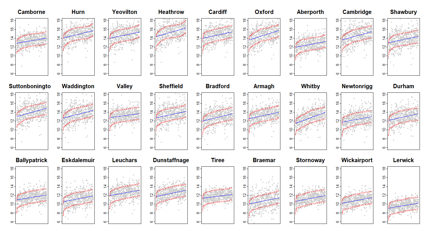
Figure 2: Joint SCBs for monthly highest temperature (°C, y-axis) in 27 stations from January 1979 to December 2020 (x-axis). The points represent the time series adjusted by removing seasonal effects. The solid lines represent quadratic trend fitted by constrained LSE. The dotted and dashed lines represent the 90% and 95% joint SCBs respectively. Notice that the solid line is not covered by the 95% SCB in Cardiff, Durham, Shawbury and Newtonrigg.

Our joint SCBs can be further used to test whether the maximum temperature at time $t=t_{1}$ has significantly exceeded the maximum temperature at $t=t_{0}$ by a given amount, through testing the null hypothesis

$$H_{0}:m_{k}(t_{1})-m_{k}(t_{0})\leq C,~{}~{}~{}\forall k=1,\dots,p,$$

under the assumption that $m_{k}(t)$ is smoothly increasing for $1\leq k\leq p$. The value of $C$ can be determined based on the field knowledge. In the context of global warming, a report from IPCC (2022) has identified about $0.5$°C difference in temperature extremes over time spans. To investigate whether the finding in IPCC (2022) appears significantly in the UK data, we set $C=0.5$, and make the time $t_{0}$ and $t_{1}$ correspond to the beginning (1979) and end (2020) of our data set. Based on our level (1-$\alpha$) joint SCBs $\hat{\mathbf{m}}_{I}\pm\hat{q}_{1-\alpha}\mathcal{B}_{p}$ obtained from Algorithm 4.3, we shall reject $H_{0}$ at level $\alpha$ if $\mathbf{m}(t)$ could not be covered by $\hat{\mathbf{m}}_{I}\pm\hat{q}_{1-\alpha}\mathcal{B}_{p}$, i.e.

$$(\hat{m}_{I,k}(t_{1})-\hat{q}_{1-\alpha})-(\hat{m}_{I,k}(t_{0})+\hat{q}_{1-\alpha})>C,\text{ for some $k\in\{1,\dots,p\}.$}$$ (8.1)

For this data, we find the highest confidence level at which (8.1) holds is $1-\alpha=97.3\%$ (see Figure 3), thus we reject the null hypothesis with a small $p$-value of $1-0.973=0.027$. In fact, Figure 3 shows that for Heathrow station $(\hat{m}_{I,heathrow}(t_{1})-\hat{q}_{1-\alpha})-(\hat{m}_{I,heathrow}(t_{0})+\hat{q}_{1-\alpha})>C$, which rejects the null hypothesis.

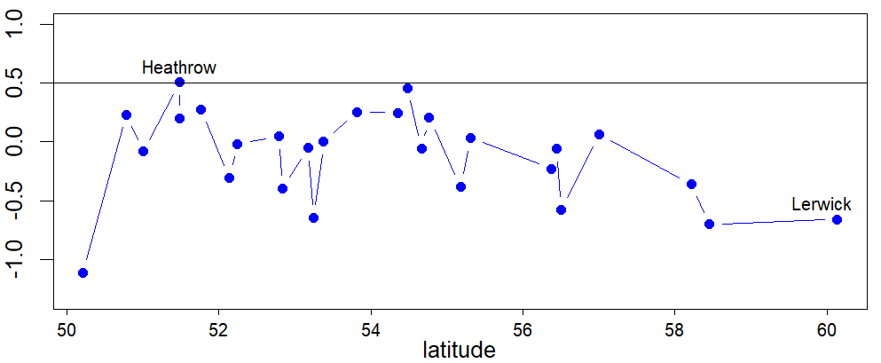
Figure 3: $(\hat{m}_{I,k}(t_{1})-\hat{q}_{1-\alpha})-(\hat{m}_{I,k}(t_{0})+\hat{q}_{1-\alpha})$ with $\alpha=0.027$ (y-axis) for each station ordered according to the latitude (x-axis).

Our results indicate a faster warming rate in most southern parts of the UK comparing to the northern parts, exemplified by the difference between Heathrow in the south and Lerwick in the north in Figure 3. This phenomenon may be attributed to the fact that the stations in southern UK areas are often near cities or densely populated regions, and consequently experience more significant warming effects caused by more energy consumption and greenhouse gas emissions, severe urban heat island effect, and so on. We shall further investigate the climate data from Heathrow and Lerwick in the next section.

8.2 Temperature-sunshine analysis

In this section we investigate the relationship between sunshine duration and atmospheric temperature, especially how the former impacts the latter. Specifically, we consider the following time-varying coefficient linear model for the maximum temperature and sunshine duration:

$$T_{max,i}=m_{0}(t_{i})+m_{1}(t_{i})SD_{i}+e_{i},\quad i=1,\dots,n,$$ (8.2)

where $(T_{max,i})_{i=1}^{n}$ is the series of monthly maximum temperature and $(SD_{i})_{i=1}^{n}$ represents the series of monthly sunshine duration. In model (8.2), we assume $m_{1}(t)$ is strictly increasing which has been supported by evidence from climatology research. For example, Matuszko & Weglarczyk (2015) finds more significant and higher correlation coefficients between sunshine duration and air temperature in 1954-2012 than 1884-1953.

We investigate (8.2) using the historical data from Heathrow and Lerwick, separately. By methodology proposed in Section 5, we obtain the monotone estimates as well as the corresponding SCB for the coefficient $m_{1}(t)$, which can be used to test whether the sunshine duration always has a positive effect on temperature including monthly maximum. For this purpose, we consider the null hypothesis $H_{0}:\inf_{t\in\hat{\mathcal{T}}}m_{1}(t)\leq 0$, and test this null using the SCB constructed by Algorithm 5. Alternative SCBs that could be used for testing $H_{0}$ include Zhou & Wu (2010) which imposes no monotone constraints, and the conservative monotone SCB obtained by modifying Zhou & Wu (2010) using order-preserving improving procedure, see for example Chernozhukov et al. (2009).

In Figure 4, we compare 90% SCB constructed by our Algorithm 5, and the SCB generated by Zhou & Wu (2010) and its order-preserving modification using Chernozhukov et al. (2009) for $m_{1}(t)$ in (8.2), based on the data collected from Heathrow and Lerwick stations. The results demonstrate that both Zhou & Wu (2010) and Chernozhukov et al. (2009) fail to reject the null hypothesis $H_{0}$ at 10% significance level for Heathrow station. Notice that Zhou & Wu (2010) does not guarantee monotone constraints while Chernozhukov et al. (2009) yields conservative coverage, as a consequence, testing procedures using the two SCBs for $H_{0}$ might lack power when the underlying time-varying coefficient is monotone as in our scenario. In contrast, our SCB based on the monotone rearranged estimator generated by Algorithm 5, suggests a significant positive relationship between sunshine duration and temperature at 90% confidence level in Heathrow. Moreover, all three considered SCB fail to reject the null hypothesis at 10% significance level in Lerwick.

The difference in the testing results between Heathrow and Lerwick in Figure 4 may be due to the geographic reason. This difference shows the temperature mechanism can vary in regional scale, even though on a global scale the sun is the fundamental source of heat on Earth. Specifically, Heathrow is situated adjacent to the city of London, where human activities and urbanization may have diminished the environment’s capacity to adjust. As a result, sunshine duration has a significant impact on the weather patterns in Heathrow. On the other hand, Lerwick is located approximately 123 miles off the north coast of the Scottish mainland. Its climate is mainly influenced by maritime factors, which means the effect of sunshine duration on temperature is less pronounced compared with Heathrow.

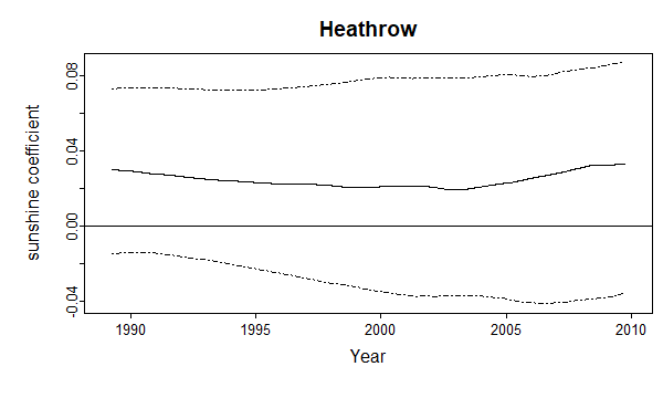
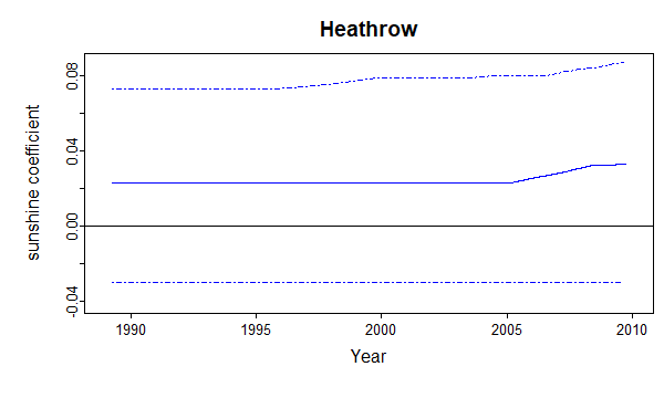
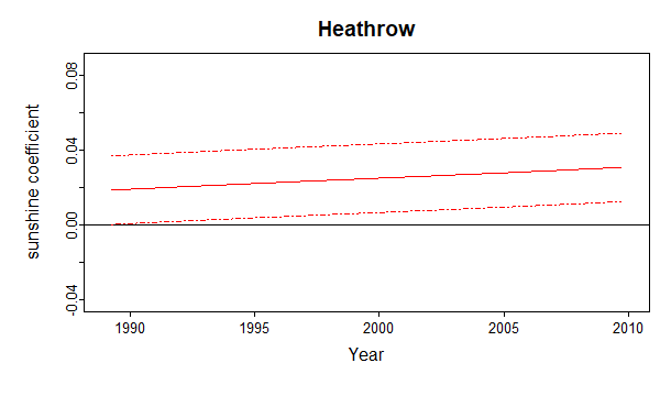
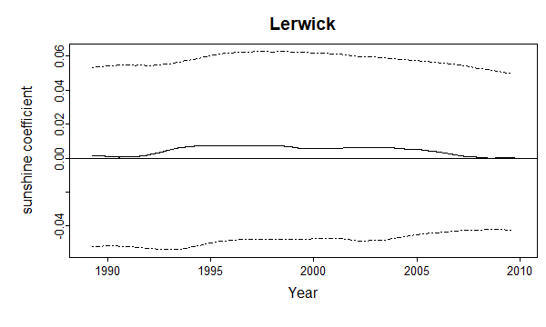
(a)

(b)

(c)

Figure 4: 90% SCBs (dotted) and estimations (solid) on $m_{1}(t)$ in model (8.2) for Heathrow and Lerwick. SCB in (a) is derived by Zhou & Wu (2010) which does not consider the monotone constraint. SCB in (b) is the order-preserving modification of Zhou & Wu (2010) via Chernozhukov et al. (2009), which is conservative. SCB in (c) is generated by Algorithm 5.

9 Discussion and future work

In this paper, we develop a simultaneous inference framework for monotone and smoothly time-varying functions based on the nonparametric and monotone rearrangement estimator, allowing complex temporal dynamics. We study the inference problem in detail for two important and practical scenarios, namely, the high-dimensional trends model and the time-varying coefficient linear model. In these contexts, we have developed Gaussian approximations and the associated bootstrap algorithms for constructing joint SCBs. Importantly, the proposed joint SCBs are asymptotically correct. In the numerical study, our proposed joint SCBs also show the narrowest width compared with the existing method.

For future work, a promising avenue could be connecting the monotone regression technique with quantile regression that has garnered attention in previous work, as demonstrated by for example Dette & Volgushev (2008), Huang (2017), and Dhar & Wu (2023). Another valuable direction is to align our work with monotone regression that has multivariate index sets $\mathbf{t}\in[0,1]^{p}$. This line of research has drawn considerable attention recently, see for example Chatterjee et al. (2018), Deng et al. (2021).

SUPPLEMENTARY MATERIAL

A Proofs.

Supplement providing proofs of main results in this paper with essential lemmas and auxiliary results.

B Appendix.

Supplement containing general example of high-dimensional error process for assumption verification, additional simulation for SCB comparison, and detailed information for stations we used in empirical study.

Supplement to “Simultaneous inference for monotone and smoothly time-varying functions under complex temporal dynamics”

This supplementary material will provide detailed proofs in Section A and a further appendix in Section B. Section A contains proofs of the theorems and propositions in main paper with essential lemmas and auxiliary results. Section B displays general example, further discussion, additional simulation report and detailed information for stations we used in empirical study. In particular, additional simulation in Section B.3 compares the width of SCB obtained by our method with various alternative SCBs and finds that our SCB enjoys the narrowest width while maintaining confidence levels.

A Proofs

For $k\in\mathbb{Z}$, define the projection operator $\mathcal{P}_{k}\cdot=\mathbb{E}\left(\cdot\mid\mathcal{F}_{k}\right)-\mathbb{E}\left(\cdot\mid\mathcal{F}_{k-1}\right)$. We write $a_{n}\lesssim b_{n}$($a_{n}\gtrsim b_{n}$) to mean that there exists a universal constant $C>0$ such that $a_{n}\leq Cb_{n}$($Ca_{n}\geq b_{n}$) for all $n$. For set $A$, denote $\#A$ as the number of elements in $A$. For matrix $A,\operatorname{tr}(A)$ denotes the trace of $A$, and $\|A\|_{\operatorname{tr},p}=:\operatorname{tr}\left(\left(A^{\top}A\right)^{p/2}\right)^{1/p}$ is the Schatten norm of order $p$. $\|\cdot\|_{\operatorname{tr}}$ refers to $\|\cdot\|_{\operatorname{tr},1}$ if no extra clarification, which is known as the trace norm. If no confusion is caused, we shall use $\mathbf{\Sigma}_{i}$ to represent the long-run covariance function $\mathbf{\Sigma}_{\mathbf{G}}(i)$.

Introduce $m_{N}(t)$ as auxiliary function towards $m(t)$, which is defined by the inverse of function below:

$$m_{N}^{-1}(s)=:\int_{-\infty}^{s}\frac{1}{Nh_{d}}\sum_{i=1}^{N}K_{d}\left(\frac{m(i/N)-u}{h_{d}}\right)\mathrm{d}u.$$ (A.1)

The error between $m_{N}^{-1}$ and $m^{-1}$ can be viewed as the error of monotone rearrangement step which is nonrandom and totally depends on $N$ and $h_{d}$. Dette et al. (2006) has proposed Lemmas to show $m_{N}(t)$ is pretty close to true $m(t)$ pointwise and we give a generalized global version Lemma A.10 in auxiliary.

If $m$ is decreasing, we shall firstly reverse the observation data and follow the sane procedure in increasing situation to obtain $\hat{m}_{I}$. It should be mentioned that $\hat{m}_{I}$ is defined from its inverse

$$\hat{m}_{I}^{-1}(s)=:\int_{-\infty}^{s}\frac{1}{Nh_{d}}\sum_{i=1}^{N}K_{d}\left(\frac{\widehat{m_{-}}(i/N)-u}{h_{d}}\right),$$

where $\widehat{m_{-}}$ is the local linear estimator from the origin sample $-y_{i},i=1,\dots,n$. Therefore, $|\hat{m}_{I}-(-m)|$ can follow all the theorems in increasing situation. In this way, we take $-\hat{m}_{I}$ as the decreasing estiamtor towards true function $m$, then we can find that simultaneous results for $|-\hat{m}_{I}-m|$ is actually equivalent to the increasing situation $|\hat{m}_{I}-(-m)|$.

For $p$-dimensional vector function $\mathbf{m}(t)=(m_{1}(t),\dots,m_{p}(t))^{\top}$, we define $\mathbf{m}_{N}(t)=:(m_{N,1}(t),\dots,m_{N,p}(t))^{\top}$ where $m_{N,k}$ is the inverse of $m_{N,k}^{-1}$ defined by replacing $m(i/N),h_{d}$ in (A.1) as $m_{k}(i/N),h_{d,k}$ respectively.

A.1 Proofs of main results

A.1.1 Proof of Lemma A.1

Lemma A.1.

Suppose Assumptions (A1)-(A2), (C1)-(C2) and $\max_{1\leq k\leq p}\sup_{t\in[0,1]}|\tilde{m}_{k}(t)-m_{k}(t)|=O_{p}(R_{n})$ are satisfied, then

$$\max_{1\leq k\leq p}\sup_{t\in\hat{\mathcal{T}}}|m_{N,k}(t)-\hat{m}_{I,k}(t)-\frac{\hat{m}_{I,k}^{-1}-m_{N,k}^{-1}}{\left(m_{k}^{-1}\right)^{\prime}}\circ m_{k}(t)|=O_{p}(R_{n}^{2}/h_{d}).$$ (A.2)

• We firstly introduce an operator which maps an increasing function $m$ to its “quantile” $m^{-1}(t)$. Let $\mathcal{M}$ be the function class such that all $H\in\mathcal{M}$ are strictly increasing and exist second order derivative. For a fixed $t$ which lies in the interior of $H$’s image, consider the functional

  $$\Phi_{t}:\left\{\begin{array}[]{l}\mathcal{M}\mapsto\mathbb{R}\\ H\mapsto H^{-1}(t)\end{array}\right.$$

  and define for $H_{1},H_{2}\in\mathcal{M}$ the function

  $$Q_{t}:\left\{\begin{array}[]{l}{[0,1]\mapsto\mathbb{R}}\\ \lambda\mapsto\Phi_{t}\left(H_{1}+\lambda\left(H_{2}-H_{1}\right)\right).\end{array}\right.$$

  Let $F(x,y)=(H_{1}+x(H_{2}-H_{1}))(y)-t$, then $Q_{t}(\lambda)$ satisfies $F(\lambda,Q_{t}(\lambda))=0$. Then

  $$Q_{t}^{\prime}(\lambda)=-\frac{H_{2}-H_{1}}{h_{1}+\lambda\left(h_{2}-h_{1}\right)}\circ\left(H_{1}+\lambda\left(H_{2}-H_{1}\right)\right)^{-1}(t),$$ (A.3)

  where $h_{1},h_{2}$ are the derivatives of $H_{1},H_{2}$. Moreover, we have

  $$Q_{t}^{\prime\prime}(\lambda)=Q_{t}^{\prime}(\lambda)\cdot\left\{\frac{-2\left(h_{2}-h_{1}\right)}{h_{1}+\lambda\left(h_{2}-h_{1}\right)}+\frac{\left(H_{2}-H_{1}\right)\left(h_{1}^{\prime}+\lambda\left(h_{2}^{\prime}-h_{1}^{\prime}\right)\right)}{\left\{h_{1}+\lambda\left(h_{2}-h_{1}\right)\right\}^{2}}\right\}\circ Q_{t}(\lambda),$$ (A.4)

  Let $H_{2}=\hat{m}_{I,k}^{-1}$ and $H_{1}=m_{N,k}^{-1}$ in (A.3) and (A.4) and use the fact $Q_{t}(1)=\Phi_{t}(H_{2}),Q_{t}(0)=\Phi_{t}(H_{1})$, by Lagrange’s

  $$\hat{m}_{I,k}(t)-m_{N,k}(t)=Q_{t}(1)-Q_{t}(0)=Q_{t}^{\prime}(0)+\frac{1}{2}Q_{t}^{\prime\prime}(\lambda_{t}^{*})=A_{N,k}(t)+\frac{1}{2}B_{N,k}(t),$$ (A.5)

  where $\lambda_{t}^{*}\in[0,1]$ and

  $$A_{N,k}(t)= -\frac{\hat{m}_{I,k}^{-1}-m_{N,k}^{-1}}{\left(m_{N,k}^{-1}\right)^{\prime}}\circ m_{N,k}(t),$$

  $$B_{N,k}(t)= \frac{2\left(\hat{m}_{I,k}^{-1}-m_{N,k}^{-1}\right)\left(\hat{m}_{I,k}^{-1}-m_{N,k}^{-1}\right)^{\prime}}{\left\{\left(m_{N,k}^{-1}+\lambda_{t}^{*}\left(\hat{m}_{I,k}^{-1}-m_{N,k}^{-1}\right)\right)^{\prime}\right\}^{2}}\circ\left(m_{N,k}^{-1}+\lambda_{t}^{*}\left(\hat{m}_{I,k}^{-1}-m_{N,k}^{-1}\right)\right)^{-1}(t)$$

  $$-\frac{\left(\hat{m}_{I,k}^{-1}-m_{N,k}^{-1}\right)^{2}\left(m_{N,k}^{-1}+\lambda_{t}^{*}\left(\hat{m}_{I,k}^{-1}-m_{N,k}^{-1}\right)\right)^{\prime\prime}}{\left\{\left(\hat{m}_{I}^{-1}+\lambda_{t}^{*}\left(\hat{m}_{I,k}^{-1}-m_{N,k}^{-1}\right)\right)^{\prime}\right\}^{3}}\circ\left(m_{N,k}^{-1}+\lambda_{t}^{*}\left(\hat{m}_{I,k}^{-1}-m_{N,k}^{-1}\right)\right)^{-1}(t).$$

  Then we prove following two assertions

  $$\max_{1\leq k\leq p}\sup_{t\in\hat{\mathcal{T}}}|A_{N,k}(t)+\frac{\hat{m}_{I,k}^{-1}-m_{N,k}^{-1}}{\left(m_{k}^{-1}\right)^{\prime}}\circ m_{k}(t)|=O_{p}\left(R_{n}h_{d}\right),$$ (A.6)

  $$\max_{1\leq k\leq p}\sup_{t\in\hat{\mathcal{T}}}|B_{N,k}(t)|=O_{p}\left(R_{n}^{2}/h_{d}\right).$$ (A.7)

  Firstly, we prove (A.6). By Lagrange’s mean value

  $$(\hat{m}_{I,k}^{-1}-m_{N,k}^{-1})\circ m_{N,k}(t)=(\hat{m}_{I,k}^{-1}-m_{N,k}^{-1})\circ m_{k}(t)+\left[(\hat{m}_{I,k}^{-1}-m_{N,k}^{-1})^{\prime}(\xi_{t,N,k})\right]\cdot\left(m_{N,k}(t)-m_{k}(t)\right),$$ (A.8)

  where $\xi_{t,N,k}$ is between $m_{k}(t)$ and $m_{N,k}(t)$. By (A.87) in Lemma A.8

  $$\max_{1\leq k\leq p}\sup_{t\in\hat{\mathcal{T}}}|(\hat{m}_{I,k}^{-1}-m_{N,k}^{-1})^{\prime}(\xi_{t,N,k})|\leq\max_{1\leq k\leq p}\sup_{t\in\mathbb{R}}|(\hat{m}_{I,k}^{-1}-m_{N,k}^{-1})^{\prime}(t)|=O_{p}\left(\frac{R_{n}}{h_{d}}\right).$$ (A.9)

  Combine (A.9) and (A.97) in Lemma A.10, the (A.8) can be written as

  $$\max_{1\leq k\leq p}\sup_{t\in\hat{\mathcal{T}}}|(\hat{m}_{I,k}^{-1}-m_{N,k}^{-1})\circ m_{N,k}(t)-(\hat{m}_{I,k}^{-1}-m_{N,k}^{-1})\circ m_{k}(t)|=O_{p}\left(R_{n}h_{d}\right).$$ (A.10)

  For $B_{N,k}$, we decompose $B_{N,k}=2B_{N1,k}-B_{N2,k}$

  $$B_{N1,k}(t) =\frac{\left(\hat{m}_{I,k}^{-1}-m_{N,k}^{-1}\right)\left(\hat{m}_{I,k}^{-1}-m_{N,k}^{-1}\right)^{\prime}}{\left\{\left[m_{N,k}^{-1}+\lambda_{t}^{*}\left(\hat{m}_{I,k}^{-1}-m_{N,k}^{-1}\right)\right]^{\prime}\right\}^{2}}\circ t_{n},$$

  $$B_{N2,k}(t) =\frac{\left(\hat{m}_{I,k}^{-1}-m_{N,k}^{-1}\right)^{2}\left(m_{N}^{-1}+\lambda_{t}^{*}\left(\hat{m}_{I,k}^{-1}-m_{N,k}^{-1}\right)\right)^{\prime\prime}}{\left\{\left[\hat{m}_{I,k}^{-1}+\lambda_{t}^{*}\left(\hat{m}_{I,k}^{-1}-m_{N,k}^{-1}\right)\right]^{\prime}\right\}^{3}}\circ t_{n},$$

  where $t_{n}=(m_{N,k}^{-1}+\lambda_{t}^{*}(\hat{m}_{I,k}^{-1}-m_{N,k}^{-1}))^{-1}(t)$. Note that $t_{n}\rightarrow_{p}m_{N,k}(t)$ and

  $$\max_{1\leq k\leq p}\sup_{t\in\mathbb{R}}|(m_{N,k}^{-1})^{\prime\prime}(t)|=\max_{1\leq k\leq p}\frac{1}{h_{d,k}}\sup_{t\in\mathbb{R}}|\frac{1}{Nh_{d,k}}\sum_{i=1}^{N}K_{d}^{\prime}\left(\frac{m_{k}(i/N)-t}{h_{d,k}}\right)|=O(\frac{1}{h_{d}}),$$

  together with (A.86), (A.87), (A.88) in Lemma A.8 and Lemma A.9,

  $$\max_{1\leq k\leq p}\sup_{t\in\hat{\mathcal{T}}}|B_{N1,k}(t)|=O_{p}\left(\frac{R_{n}^{2}}{h_{d}}\right),\quad\max_{1\leq k\leq p}\sup_{t\in\hat{\mathcal{T}}}|B_{N2,k}(t)|=O_{p}\left(\frac{R_{n}^{2}}{h_{d}}\right).$$ (A.11)

  Combining (A.10) and (A.11), we can obtain the desired rate in (A.6) and (A.7). Finally, combining (A.5), (A.6) and (A.7), it immediately yields

  $$\max_{1\leq k\leq p}\sup_{t\in\hat{\mathcal{T}}}|m_{N,k}(t)-\hat{m}_{I,k}(t)-\frac{\hat{m}_{I,k}^{-1}-m_{N,k}^{-1}}{\left(m_{k}^{-1}\right)^{\prime}}\circ m_{k}(t)|=O_{p}(R_{n}^{2}/h_{d}).$$ (A.12)

  ∎

A.1.2 Proof of Proposition 4.1

• For $k=1,2,\dots,p$, denote

  $$\mathcal{S}_{k}^{(0)}(t)=:\frac{\hat{m}_{I,k}^{-1}-m_{Nk}^{-1}}{(m_{k}^{-1})^{\prime}}\circ m_{k}(t).$$

  By Lemma A.12, we have $\max_{1\leq k\leq p}\sup_{t\in[0,1]}|\tilde{m}_{k}(t)-m_{k}(t)|=O_{p}(R_{n})$, then using Lemma A.1, we shall have

  $$\max_{1\leq k\leq p}\sup_{t\in\hat{\mathcal{T}}}|m_{N,k}(t)-\hat{{m}}_{I,k}(t)-\mathcal{S}_{k}^{(0)}(t)|=O_{p}(R_{n}^{2}/h_{d}).$$ (A.13)

  By Taylor’s expansion

  $$\hat{m}_{I,k}^{-1}(t)-m_{N,k}^{-1}(t) =\frac{1}{Nh_{d,k}^{2}}\int_{-\infty}^{t}\sum_{i=1}^{N}(\tilde{m}_{k}(i/N)-m_{k}(i/N))K_{d}^{\prime}\left(\frac{m_{k}(i/N)-u}{h_{d,k}}\right)du$$

  $$+\frac{1}{2Nh_{d,k}^{3}}\int_{-\infty}^{t}\sum_{i=1}^{N}(\tilde{m}_{k}(i/N)-m_{k}(i/N))^{2}K_{d}^{\prime\prime}\left(\frac{\eta_{i,N,k}-u}{h_{d,k}}\right)du,$$ (A.14)

  for some $\eta_{i,N,k}$ between $\hat{m}_{k}(i/N)$ and $m_{k}(i/N)$. By Lemma A.12, uniformly $t\in(m(0),m(1))$, the second line in (A.14) is of rate $O_{p}(R_{n}^{2}/h_{d})$. Then based on (A.14), we have

  $$\max_{1\leq k\leq p}\sup_{t\in\mathbb{R}}|\hat{m}_{I,k}^{-1}(t)-m_{N,k}^{-1}(t)+\frac{1}{Nh_{d,k}}\sum_{i=1}^{N}(\tilde{m}_{k}(i/N)-m_{k}(i/N))K_{d}\left(\frac{m_{k}(i/N)-t}{h_{d,k}}\right)|=O_{p}(R_{n}^{2}/h_{d}).$$ (A.15)

  Combining definition of $\mathcal{S}_{k}^{(0)}(t)$ and (A.15), we have

  $$\max_{1\leq k\leq p}\sup_{t\in\hat{\mathcal{T}}}|\mathcal{S}_{k}^{(0)}(t)-\frac{m_{k}^{\prime}(t)}{Nh_{d,k}}\sum_{i=1}^{N}(\tilde{m}_{k}(i/N)-m_{k}(i/N))K_{d}\left(\frac{m_{k}(i/N)-m_{k}(t)}{h_{d,k}}\right)|=O_{p}(R_{n}^{2}/h_{d}).$$ (A.16)

  By Lemma A.5, on a richer space, there exists independent $\mathbf{V}_{j}\sim N_{p}(0,\mathbf{\Sigma}_{j})$, $j=1,\dots,n$, such that for $\mathbf{e}_{l}$ defined in (4.1)

  $$\max_{k\leq n}\left|\sum_{l=1}^{k}(\mathbf{e}_{l}-\mathbf{V}_{l})\right|=O_{p}\left(\Theta(p)\sqrt{n\log n}\left(\frac{p}{n}\right)^{\frac{q-2}{6q-4}}\right).$$ (A.17)

  Denote vectors $\mathcal{E}^{(0)}(t)=(\mathcal{E}_{1}^{(0)}(t),\dots,\mathcal{E}_{p}^{(0)}(t))^{\top}$ and $\mathcal{V}^{(0)}(t)=(\mathcal{V}_{1}^{(0)}(t),\dots,\mathcal{V}_{p}^{(0)}(t))^{\top}$,

  $$\mathcal{E}^{(0)}(t)=:\mathcal{M}(t)\sum_{j=1}^{n}\sum_{i=1}^{N}\mathcal{K}_{d}(t,i/N)\mathcal{K}_{r}(j/n,i/N)\mathbf{e}_{j},$$

  $$\mathcal{V}^{(0)}(t)=:\mathcal{M}(t)\sum_{j=1}^{n}\sum_{i=1}^{N}\mathcal{K}_{d}(t,i/N)\mathcal{K}_{r}(j/n,i/N)\mathbf{V}_{j},$$ (A.18)

  where $\mathcal{M}(t)=\operatorname{diag}\left\{m_{k}^{\prime}(t)\right\}_{k=1}^{p}$ and

  $$\mathcal{K}_{r}(j/n,i/N)=\operatorname{diag}\left\{\frac{1}{nh_{r,k}}\tilde{K}^{*}_{r}\left(\frac{j/n-i/N}{h_{r,k}},\frac{i}{N}\right)\right\}_{k=1}^{p},$$

  $$\mathcal{K}_{d}(t,i/N)=\operatorname{diag}\left\{\frac{1}{Nh_{d,k}}K_{d}\left(\frac{m_{k}(i/N)-m_{k}(t)}{h_{d,k}}\right)\right\}_{k=1}^{p}.$$

  Combining (A.16) and Lemma A.11 with jackknife bias correction, it can yield that

  $$\max_{1\leq k\leq p}\sup_{t\in\hat{\mathcal{T}}}|\mathcal{S}_{k}^{(0)}(t)-\mathcal{E}_{k}^{(0)}(t)|=O_{p}\left(\frac{R_{n}^{2}}{h_{d}}+h_{r}^{3}+\frac{1}{nh_{r}}\right).$$ (A.19)

  Recall $\nu_{l,k}(t)$ defined in (4.8), for $\kappa_{l}=:\int|x|^{l}K_{r}(x)\mathrm{d}x$, using the fact $\kappa_{2}-\kappa_{1}^{2}>0$, we have

  $$\inf_{t\in[0,1]}|\nu_{0,k}(t)\nu_{2,k}(t)-\nu^{2}_{1,k}(t)| \geq\frac{1}{2}\cdot\frac{1}{2}\int_{-1}^{1}x^{2}K_{r}(x)\mathrm{d}x-\left(\frac{1}{2}\int_{-1}^{1}|x|K_{r}(x)\mathrm{d}x\right)^{2},$$

  $$\geq\frac{1}{4}(\kappa_{2}-\kappa_{1}^{2}).$$ (A.20)

  For $c_{k}(t)=:\nu_{0,k}(t)\nu_{2,k}(t)-\nu^{2}_{1,k}(t)$, we have $\inf_{t\in[0,1]}c_{k}(t)\geq(\kappa_{2}-\kappa_{1}^{2})/4$, thus $\tilde{K}^{*}$ defined in (4.7) is bounded. Using summation by parts, we have

  $$\max_{1\leq k\leq p}\sup_{t\in\hat{\mathcal{T}}}|\mathcal{V}_{k}^{(0)}(t)-\mathcal{E}_{k}^{(0)}(t)|$$

  $$\leq\max_{1\leq k\leq p}\sup_{t\in\hat{\mathcal{T}}}\left|\frac{m_{k}^{\prime}(t)}{Nh_{d,k}}\sum_{i=1}^{N}K_{d}\left(\frac{m_{k}(i/N)-m_{k}(t)}{h_{d,k}}\right)\frac{1}{nh_{r,k}}\sum_{j=1}^{n-1}\Delta_{j}(\tilde{K}_{r}^{*})\right|\cdot\max_{j\leq n}\left|\sum_{l=1}^{j}(\mathbf{e}_{l}-\mathbf{V}_{l})\right|$$

  $$+\max_{1\leq k\leq p}\sup_{t\in\hat{\mathcal{T}}}\left|\frac{m_{k}^{\prime}(t)}{Nh_{d,k}}\sum_{i=1}^{N}K_{d}\left(\frac{m_{k}(i/N)-m_{k}(t)}{h_{d,k}}\right)\frac{1}{nh_{r,k}}\tilde{K}^{*}\left(\frac{1-i/N}{h_{r,k}},\frac{i}{N}\right)\right|\cdot\max_{j\leq n}\left|\sum_{l=1}^{j}(\mathbf{e}_{l}-\mathbf{V}_{l})\right|$$

  $$=O_{p}\left\{\frac{\Theta(p)\sqrt{n\log n}\left(\frac{p}{n}\right)^{\frac{q-2}{6q-4}}}{nh_{r}}\right\},$$ (A.21)

  where

  $$\Delta_{j}(\tilde{K}_{r}^{*})=:\left[\tilde{K}_{r}^{*}\left(\frac{j/n-i/N}{h_{r,k}},\frac{i}{N}\right)-\tilde{K}_{r}^{*}\left(\frac{(j+1)/n-i/N}{h_{r,k}},\frac{i}{N}\right)\right]$$

  and the last line in (A.21) is obtained in view of (A.17).

  Combining (A.13), (A.19) and (A.21), we have

  $$\max_{1\leq k\leq p}\sup_{t\in\hat{\mathcal{T}}}|m_{N,k}(t)-\hat{m}_{I,k}(t)-\mathcal{V}_{k}^{(0)}(t)|=O_{p}\left\{\frac{R_{n}^{2}}{h_{d}}+\frac{\Theta(p)\sqrt{n\log n}\left(\frac{p}{n}\right)^{\frac{q-2}{6q-4}}}{nh_{r}}\right\}.$$ (A.22)

  Then by Lemma A.10, $\mathcal{V}^{(0)}(t)$ satisfies (4.6). ∎

A.1.3 Proof of Theorem 4.1

• To illustrate, we define a union rate

  $$\rho_{n}^{*}=:\frac{\Theta(p)\left(\frac{p}{n}\right)^{\frac{q-2}{6q-4}}\sqrt{n}\log n}{nh_{r}}\bigvee\frac{\sqrt{\sqrt{n\varphi_{n}p}+\varphi_{n}+p}\log(n)}{nh_{r}},$$

  where $\varphi_{n}=\Theta^{2}(p)(\sqrt{npL}+nL^{-1})+p^{3/2}L\sqrt{n}\left(\Theta(p)R_{n}+\sqrt{n}\left(h_{r}^{5}+\frac{\log^{6}(n)}{nh_{r}}\right)\right)$.

  Denote

  $$\mathcal{V}^{(1)}(t)=:\sum_{j=1}^{n}\sum_{i=1}^{N}\mathcal{W}(i/N,t)\mathcal{K}_{r}(j/n,i/N)\mathbf{V}_{j},$$

  where $\mathbf{V}_{j},j=1,\dots,n$ is the same as (A.18). Note that $\hat{Q}(k)-\hat{Q}(k-1)$ is positive semidefinite, given data, Lemma A.7 indicates that there exists independent $\mathbf{V}_{j}^{*}\sim N_{p}(0,\hat{\mathbf{Q}}(j)-\hat{\mathbf{Q}}(j-1)),j=1,\dots,n$ on a richer space s.t.

  $$\mathbb{E}\left(\max_{k=1,\ldots,n}\left|\sum_{j=1}^{k}\mathbf{V}_{j}-\sum_{j=1}^{k}\mathbf{V}^{*}_{j}\right|^{2}\,\middle|\,\mathcal{F}_{n}\right)\leq C\log(n)(\sqrt{n\varphi^{\Delta}\Phi}+\varphi^{\Delta}+\Phi)$$ (A.23)

  where

  $$\varphi^{\Delta}=\max_{k=1,\dots,n}\left\|\sum_{j=1}^{k}\mathbf{\Sigma}_{j}-\hat{\mathbf{Q}}(k)\right\|_{\operatorname{tr}},\quad\Phi=\max_{t=1,\dots,n}\|\mathbf{\Sigma}_{j}\|_{\operatorname{tr}}.$$

  Thus with summation by parts formula, given the data,

  $$\sup_{t\in\hat{\mathcal{T}}}\left|\mathcal{V}^{(1)}(t)-\mathcal{V}^{*}(t)\right| \lesssim\sup_{t\in\hat{\mathcal{T}}}\left|\sum_{i=1}^{N}\mathcal{W}(i/N,t)\sum_{j=1}^{n-1}[\mathcal{K}_{r}(j/n,i/N)-\mathcal{K}_{r}((j+1)/n,i/N)]\right|$$

  $$\cdot\max_{j=1,\ldots,n}\left|\sum_{t=1}^{j}\mathbf{V}_{t}-\sum_{t=1}^{j}\mathbf{V}^{*}_{t}\right|,$$

  $$=O_{p}\left(\frac{\sqrt{\log(n)(\sqrt{n\varphi^{\Delta}\Phi}+\varphi^{\Delta}+\Phi)}}{nh_{r}}\right),$$ (A.24)

  where the last line is obtained by using (A.23) and the fact $\sum_{i=1}^{N}\mathcal{W}(i/N,t)=I_{p}$.

  By Assumption (B4), $p\underline{\Lambda}\leq\|\Sigma(t)\|_{\operatorname{tr}}\leq p\Lambda$ for any $t\in[0,1]$, thus $\Phi\asymp p$. Note that $\varphi^{\Delta}=O_{p}(\varphi_{n})$ by Lemma A.3, then we can have

  $$\sup_{t\in\hat{\mathcal{T}}}\left|\mathcal{V}^{(1)}(t)-\mathcal{V}^{*}(t)\right|=O_{p}\left(\frac{\sqrt{\log(n)(\sqrt{n\varphi_{n}p}+\varphi_{n}+p)}}{nh_{r}}\right)=o_{p}(\rho_{n}^{*}).$$ (A.25)

  Recall the proof of Proposition 4.1, it has shown that $\mathcal{V}^{(0)}(t)$ defined in (A.18) satisfies (4.6). Therefore, Theorem 4.1 can hold if

  $$\sup_{x\in\mathbb{R}}\left|\mathbb{P}\left\{\max_{1\leq k\leq p}\sup_{t\in\hat{\mathcal{T}}}\left|\mathcal{V}^{(0)}_{k}(t)\right|\leq x\right\}-\mathbb{P}\left\{\max_{1\leq k\leq p}\sup_{t\in\hat{\mathcal{T}}}\left|\mathcal{V}^{*}_{k}(t)\right|\leq x\,\middle|\,\mathcal{F}_{n}\right\}\right|\rightarrow_{p}0.$$

  By Lemma A.15,

  $$\sup_{x\in\mathbb{R}}\left|\mathbb{P}\left\{\max_{1\leq k\leq p}\sup_{t\in\hat{\mathcal{T}}}\left|\mathcal{V}^{(0)}_{k}(t)\right|\leq x\right\}-\mathbb{P}\left\{\max_{1\leq k\leq p}\sup_{t\in\hat{\mathcal{T}}}\left|\mathcal{V}^{*}_{k}(t)\right|\leq x\,\middle|\,\mathcal{F}_{n}\right\}\right|,$$

  $$\lesssim\sup_{x\in\mathbb{R}}\left|\mathbb{P}\left\{\max_{1\leq k\leq p}\sup_{t\in\hat{\mathcal{T}}}\left|\mathcal{V}_{k}^{(0)}(t)\right|\leq x\right\}-\mathbb{P}\left\{\max_{1\leq k\leq p}\sup_{t\in\hat{\mathcal{T}}}\left|\mathcal{V}_{k}^{(1)}(t)\right|\leq x\right\}\right|$$

  $$+\mathbb{P}\left\{\sup_{t\in\hat{\mathcal{T}}}\left|\mathcal{V}_{k}^{(1)}(t)-\mathcal{V}_{k}^{*}(t)\right|>\rho_{n}^{*}\,\middle|\,\mathcal{F}_{n}\right\}+\sup_{x\in\mathbb{R}}\mathbb{P}\left\{\left|\max_{1\leq k\leq p}\sup_{t\in\hat{\mathcal{T}}}|\mathcal{V}^{(0)}_{k}(t)|-x\right|\leq\rho_{n}^{*}\right\},$$

  $$\lesssim\mathcal{I}_{1}+\mathcal{I}_{2}+\mathcal{I}_{3},$$

  where

  $$\mathcal{I}_{1} =\mathbb{P}\left\{\max_{1\leq k\leq p}\sup_{t\in\hat{\mathcal{T}}}\left|\mathcal{V}_{k}^{(0)}(t)-\mathcal{V}_{k}^{(1)}(t)\right|>\rho_{n}^{*}\right\},$$

  $$\mathcal{I}_{2} =\sup_{x\in\mathbb{R}}\mathbb{P}\left\{\left|\max_{1\leq k\leq p}\sup_{t\in\hat{\mathcal{T}}}|\mathcal{V}_{k}^{(0)}(t)|-x\right|\leq\rho_{n}^{*}\right\},$$ (A.26)

  $$\mathcal{I}_{3} =\mathbb{P}\left\{\max_{1\leq k\leq p}\sup_{t\in\hat{\mathcal{T}}}\left|\mathcal{V}_{k}^{(1)}(t)-\mathcal{V}_{k}^{*}(t)\right|>\rho_{n}^{*}\,\middle|\,\mathcal{F}_{n}\right\}.$$ (A.27)

  Note that $\mathcal{I}_{3}$ converges to zero in probability by (A.25), then we only need to bound $\mathcal{I}_{1}$ and $\mathcal{I}_{2}$ in separately two steps.

  • Step 1

    $$\max_{1\leq k\leq p}\sup_{t\in\hat{\mathcal{T}}}\left|\mathcal{V}_{k}^{(0)}(t)-\mathcal{V}_{k}^{(1)}(t)\right|=o_{p}(\rho_{n}^{*}).$$ (A.28)

  • Step 2

    $$\sup_{x\in\mathbb{R}}\mathbb{P}\left\{x-\rho_{n}^{*}\leq\max_{1\leq k\leq n}\sup_{t\in\hat{\mathcal{T}}}|\mathcal{V}^{(0)}_{k}(t)|\leq x+\rho_{n}^{*}\right\}=o(1).$$ (A.29)

Step 1.

Firstly, we consider another form of stochastic expansion on $m_{I,k}-m_{N,k}$. Use the same technique in (A.5) but swap $\hat{m}_{I,k}^{-1}$ and $m_{N,k}^{-1}$ i.e. $H_{2}=m_{N,k}^{-1}$ and $H_{1}=\hat{m}_{I,k}^{-1}$, then by (A.3) and (A.4), for some $\lambda_{t}^{**}\in[0,1]$,

$$m_{N,k}(t)-\hat{m}_{I,k}(t)=\tilde{A}_{N,k}(t)+\frac{1}{2}\tilde{B}_{N,k}(t)$$ (A.30)

$$\tilde{A}_{N,k}(t) =-\frac{m_{N,k}^{-1}-\hat{m}_{I,k}^{-1}}{\left(\hat{m}_{I,k}^{-1}\right)^{\prime}}\circ\hat{m}_{I,k}(t),$$

$$\tilde{B}_{N,k}(t) =\frac{2\left(m_{N,k}^{-1}-\hat{m}_{I,k}^{-1}\right)\left(m_{N,k}^{-1}-\hat{m}_{I,k}^{-1}\right)^{\prime}}{\left\{\left(m_{I,k}^{-1}+\lambda_{t}^{**}\left(\hat{m}_{N,k}^{-1}-m_{I,k}^{-1}\right)\right)^{\prime}\right\}^{2}}\circ\left(m_{I,k}^{-1}+\lambda_{t}^{**}\left(\hat{m}_{N,k}^{-1}-m_{I,k}^{-1}\right)\right)^{-1}(t)$$

$$-\frac{\left(\hat{m}_{N,k}^{-1}-m_{I,k}^{-1}\right)^{2}\left(m_{I,k}^{-1}+\lambda_{t}^{**}\left(\hat{m}_{N,k}^{-1}-m_{I,k}^{-1}\right)\right)^{\prime\prime}}{\left\{\left(\hat{m}_{N,k}^{-1}+\lambda_{t}^{**}\left(\hat{m}_{N,k}^{-1}-m_{I,k}^{-1}\right)\right)^{\prime}\right\}^{3}}\circ\left(m_{I,k}^{-1}+\lambda_{t}^{**}\left(\hat{m}_{N,k}^{-1}-m_{I,k}^{-1}\right)\right)^{-1}(t).$$

By similar arguments in the proof of Lemma A.1 and Proposition 4.1, we can show that

$$\max_{1\leq k\leq p}\sup_{t\in\hat{\mathcal{T}}}|\tilde{B}_{N,k}(t)|=O_{p}(R_{n}^{2}/h_{d}).$$ (A.31)

Note that

$$(\hat{m}_{I,k}^{-1})^{\prime}(t)=\frac{d}{dt}\left\{\frac{1}{Nh_{d,k}}\sum_{i=1}^{N}\int_{-\infty}^{t}K_{d}\left(\frac{\tilde{m}_{k}(i/N)-u}{h_{d}}\right)du\right\}=\frac{1}{Nh_{d,k}}\sum_{i=1}^{N}K_{d}\left(\frac{\tilde{m}_{k}(i/N)-t}{h_{d,k}}\right),$$

thus

$$(\hat{m}_{I,k}^{-1})^{\prime}\circ\hat{m}_{I,k}(t)=\frac{1}{Nh_{d,k}}\sum_{i=1}^{N}K_{d}\left(\frac{\tilde{m}_{k}(i/N)-\hat{m}_{I,k}(t)}{h_{d,k}}\right).$$ (A.32)

By (A.14), for some $\eta_{i,N,k}$ between $\tilde{m}_{k}(i/N)$ and $m_{k}(i/N)$,

$$(m_{N,k}^{-1}-\hat{m}_{I,k}^{-1})\circ\hat{m}_{I,k}(t) =\frac{1}{Nh_{d,k}^{2}}\sum_{i=1}^{N}(m_{k}(i/N)-\tilde{m}_{k}(i/N))\int_{-\infty}^{\hat{m}_{I,k}(t)}K_{d}^{\prime}\left(\frac{\tilde{m}_{k}(i/N)-u}{h_{d,k}}\right)du,$$

$$+\frac{1}{2Nh_{d,k}^{3}}\sum_{i=1}^{N}({m}_{k}(i/N)-\tilde{m}_{k}(i/N))^{2}\int_{-\infty}^{\hat{m}_{I,k}(t)}K_{d}^{\prime\prime}\left(\frac{\eta_{i,N,k}-u}{h_{d,k}}\right)du,$$

together with (A.32), Lemma A.9 and Lemma A.12, we have

$$\max_{1\leq k\leq p}\sup_{t\in\hat{\mathcal{T}}}\left|\tilde{A}_{N,k}(t)-\frac{\sum_{i=1}^{N}K_{d}\left(\frac{\tilde{m}_{k}(i/N)-\hat{m}_{I,k}(t)}{h_{d,k}}\right)[\tilde{m}_{k}(i/N)-m_{k}(i/N)]}{\sum_{i=1}^{N}K_{d}\left(\frac{\tilde{m}_{k}(i/N)-\hat{m}_{I,k}(t)}{h_{d,k}}\right)}\right|=O_{p}(\frac{R_{n}^{2}}{h_{d}}).$$ (A.33)

By definition of $\hat{W}^{*}_{i,k,I}(t)$ in the algorithm, (A.33) can be written as

$$\max_{1\leq k\leq p}\sup_{t\in\hat{\mathcal{T}}}\left|\tilde{A}_{N,k}(t)-\sum_{i=1}^{N}\hat{W}_{i,k,I}^{*}(t)[\tilde{m}_{k}(i/N)-m_{k}(i/N)]\right|=O_{p}(R_{n}^{2}/h_{d}).$$ (A.34)

Combining (A.30),(A.31) and (A.34), we have

$$\max_{1\leq k\leq p}\sup_{t\in\hat{\mathcal{T}}}|m_{N,k}(t)-\hat{{m}}_{I,k}(t)-\sum_{i=1}^{N}\hat{W}_{i,k,I}^{*}(t)[\tilde{m}_{k}(i/N)-m_{k}(i/N)]|=O_{p}(R_{n}^{2}/h_{d}).$$ (A.35)

Secondly, denote vectors $\mathcal{S}^{(1)}(t)=(\mathcal{S}_{1}^{(1)}(t),\dots,\mathcal{S}_{p}^{(1)}(t))^{\top}$ and $\mathcal{E}^{(1)}(t)=(\mathcal{E}_{1}^{(1)}(t),\dots,\mathcal{E}_{p}^{(1)}(t))^{\top}$

$$\mathcal{S}^{(1)}(t)=:\sum_{i=1}^{N}\mathcal{W}(i/N,t)[\tilde{\mathbf{m}}(i/N)-\mathbf{m}(i/N)],$$

$$\mathcal{E}^{(1)}(t)=:\sum_{j=1}^{n}\sum_{i=1}^{N}\mathcal{W}(i/N,t)\mathcal{K}_{r}(j/n,i/N)\mathbf{e}_{j},$$

where $\tilde{\mathbf{m}}(t)=(\tilde{m}_{1}(t),\dots,\tilde{m}_{p}(t))^{\top}$ and $\mathcal{W}(i/N,t),\mathcal{K}_{r}(j/n,i//N)$ are defined in (4.9). Then (A.35) can be written as

$$\max_{1\leq k\leq p}\sup_{t\in\hat{\mathcal{T}}}|m_{N,k}(t)-\hat{{m}}_{I,k}(t)-\mathcal{S}_{k}^{(1)}(t)|=O_{p}(R_{n}^{2}/h_{d}).$$ (A.36)

Similar with (A.19), combining (A.36) and Lemma A.11 with jackknife bias correction, it can yield that

$$\max_{1\leq k\leq p}\sup_{t\in\hat{\mathcal{T}}}|\mathcal{S}_{k}^{(1)}(t)-\mathcal{E}_{k}^{(1)}(t)|=O_{p}\left(\frac{R_{n}^{2}}{h_{d}}+h_{r}^{3}+\frac{1}{nh_{r}}\right).$$ (A.37)

Note that $\mathcal{W}(i/N,t)>0$ and $\sum_{i=1}^{N}\mathcal{W}(i/N,t)=I_{p}$, using summation by parts and (A.17), we have

$$\max_{1\leq k\leq p}\sup_{t\in\hat{\mathcal{T}}}|\mathcal{V}_{k}^{(1)}(t)-\mathcal{E}_{k}^{(1)}(t)| \lesssim\sup_{t\in\hat{\mathcal{T}}}\left|\sum_{i=1}^{N}\mathcal{W}(i/N,t)\sum_{j=1}^{n-1}\left[\mathcal{K}_{r}(j/n,i/N)-\mathcal{K}_{r}((j+1)/n,i/N)\right]\right|$$

$$\cdot\max_{j\leq n}\left|\sum_{l=1}^{k}(\mathbf{e}_{l}-V_{l})\right|$$

$$=O_{p}\left\{\frac{\Theta(p)\sqrt{n\log n}\left(\frac{p}{n}\right)^{\frac{q-2}{6q-4}}}{nh_{r}}\right\}=o_{p}(\rho_{n}^{*}).$$ (A.38)

Combining (A.38), (A.37) and (A.36), we have

$$\max_{1\leq k\leq p}\sup_{t\in\hat{\mathcal{T}}}|m_{N,k}(t)-\hat{m}_{I,k}(t)-\mathcal{V}_{k}^{(1)}(t)|=o_{p}(\rho_{n}^{*}),$$

together with (A.22), (A.28) can hold since

$$\max_{1\leq k\leq p}\sup_{t\in\hat{\mathcal{T}}}\left|\mathcal{V}_{k}^{(0)}(t)-\mathcal{V}_{k}^{(1)}(t)\right|$$

$$\leq \max_{1\leq k\leq p}\sup_{t\in\hat{\mathcal{T}}}\left|m_{N,k}(t)-\hat{m}_{I,k}(t)-\mathcal{V}_{k}^{(0)}(t)\right|+\max_{1\leq k\leq p}\sup_{t\in\hat{\mathcal{T}}}\left|m_{N,k}(t)-\hat{m}_{I,k}(t)-\mathcal{V}_{k}^{(1)}(t)\right|=o_{p}(\rho_{n}^{*}).$$

Step 2.

Recall the definition of $\mathcal{V}^{(0)}(t)=(\mathcal{V}^{0}_{1}(t),\dots,\mathcal{V}^{(0)}_{p}(t))^{\top}$ in (A.18),

$$\mathcal{V}_{k}^{(0)}(t)=\frac{m_{k}^{\prime}(t)}{Nh_{d,k}}\sum_{i=1}^{N}K_{d}\left(\frac{m_{k}(i/N)-m_{k}(t)}{h_{d,k}}\right)\frac{1}{nh_{r}}\sum_{j=1}^{n}\tilde{K}_{r}^{*}\left(\frac{j/n-i/N}{h_{r,k}},\frac{i}{N}\right)V_{j,k}$$

where $V_{j,k}$ is the $k$-th coordinate of independent Gaussian random vector $\mathbf{V}_{j}\sim N_{p}(0,\mathbf{\Sigma}_{j}),j=1,\dots,n$. By Assumption (B4), $\underline{\Lambda}>0$ is smaller than any eigenvalues of $\mathbf{\Sigma}_{j}$ for any $j=1,2,\dots,n$, thus we have $\operatorname{Var}(V_{j,k})\geq\underline{\Lambda}$ for any $j,k$.

Firstly, we divide the Gaussian process $\sqrt{nh_{r}}\mathcal{V}^{(0)}(t)$ with discrete grids $s_{l}\in\Delta_{l}$ where $g_{n}=\lfloor{1/\Delta}\rfloor$ and $\Delta_{l}=[(l-1)\Delta,l\Delta]\cap\hat{\mathcal{T}}$. And we consider following centered Gaussian random vector in $\mathbb{R}^{(p\times g_{n})}$

$$(\sqrt{nh_{r}}\mathcal{V}^{(0)}_{1}(s_{1}),\dots,\sqrt{nh_{r}}\mathcal{V}^{(0)}_{1}(s_{g_{n}}),\dots,\sqrt{nh_{r}}\mathcal{V}^{(0)}_{p}(s_{1}),\dots,\sqrt{nh_{r}}\mathcal{V}^{(0)}_{p}(s_{g_{n}}))^{\top}.$$

For any $k,l$, note that $V_{1,k},V_{2,k},\dots,V_{n,k}$ are independent,

$$\operatorname{Var}[\sqrt{nh_{r}}\mathcal{V}_{k}^{(0)}(s_{l})]$$

$$=nh_{r}\operatorname{Var}(V_{j,k})(m_{k}^{\prime}(s_{l}))^{2}\sum_{j=1}^{n}\left[\sum_{i=1}^{N}\frac{1}{nh_{r,k}}\frac{1}{Nh_{d,k}}K_{d}(\frac{m_{k}(i/N)-m_{k}(s_{l})}{h_{d,k}})\tilde{K}_{r}^{*}\left(\frac{j/n-i/N}{h_{r,k}},\frac{i}{N}\right)\right]^{2},$$

$$\geq nh_{r}\underline{\Lambda}(m_{k}^{\prime}(s_{l}))^{2}\sum_{j=1}^{n}\left[\sum_{i=1}^{N}\frac{1}{nh_{r,k}}\frac{1}{Nh_{d,k}}K_{d}(\frac{m_{k}(i/N)-m_{k}(s_{l})}{h_{d,k}})\tilde{K}_{r}^{*}\left(\frac{j/n-i/N}{h_{r,k}},\frac{i}{N}\right)\right]^{2}.$$

Using $\min_{1\leq k\leq p}\inf_{t\in[0,1]}m_{k}^{\prime}(t)\geq M>0$ in Assumption (A2) then we can have for some constant $C>0$,

$$\operatorname{Var}[\sqrt{nh_{r}}\mathcal{V}_{k}^{(0)}(s_{l})]$$

$$\geq Cnh_{r}\underline{\Lambda}M^{2}\sum_{j=1}^{n}\left[\sum_{i=1}^{N}\frac{1}{nh_{r,k}}\frac{1}{Nh_{d,k}}K_{d}(\frac{m_{k}(i/N)-m_{k}(s_{l})}{h_{d,k}})\tilde{K}_{r}^{*}\left(\frac{j/n-i/N}{h_{r,k}},\frac{i}{N}\right)\right]^{2}$$

$$\geq C\underline{\Lambda}M^{2}\frac{h_{r}}{h_{r,k}}\iint_{[0,1]^{2}}K_{d}(\frac{m_{k}(u)-m_{k}(s_{l})}{h_{d,k}})K_{d}(\frac{m_{k}(v)-m_{k}(s_{l})}{h_{d,k}})I(u,v)\frac{\mathrm{d}u}{h_{d,k}}\frac{\mathrm{d}v}{h_{d,k}}+o(1),$$ (A.39)

where

$$I(u,v)=:\int_{0}^{1}\frac{1}{h_{r,k}}\tilde{K}_{r}^{*}\left(\frac{x-u}{h_{r,k}},u\right)\tilde{K}_{r}^{*}\left(\frac{x-v}{h_{r,k}},v\right)\mathrm{d}x.$$

Note that for $\forall u,v\in[0,1]$ s.t.

$$|m_{k}(u)-m_{N,k}(s_{l})|\leq h_{d,k}\text{ and }|m_{k}(v)-m_{N,k}(s_{l})|\leq h_{d,k},$$ (A.40)

we have $M|u-v|\leq|m_{k}(u)-m_{k}(v)|\leq|m_{k}(u)-m_{N,k}(s_{l})|+|m_{k}(v)-m_{N,k}(s_{l})|\leq 2h_{d,k}$, thus $|\frac{u-v}{h_{r,k}}|\leq\frac{2h_{d,k}}{Mh_{r,k}}$. For all $u,v\in[0,1]$ satifying (A.40), by the definition of $\tilde{K}_{r}^{*}$ in (4.7) and conclusion in (A.20) $\inf_{t\in[0,1]}c_{k}(t)\geq\frac{1}{4}(\kappa_{2}-\kappa_{1}^{2})$ where $c_{k}(t)=:\nu_{0,k}(t)\nu_{2,k}(t)-\nu^{2}_{1,k}(t)$,

$$\left|\tilde{K}_{r}^{*}\left(\frac{x-u}{h_{r,k}},u\right)-\tilde{K}_{r}^{*}\left(\frac{x-v}{h_{r,k}},v\right)\right| \leq\frac{1}{c_{k}(u)}\left|\nu_{2,k}(u)\tilde{K}_{r}(\frac{x-u}{h_{r,k}})-\nu_{2,k}(v)\tilde{K}_{r}(\frac{x-v}{h_{r,k}})\right|$$

$$+\frac{1}{c_{k}(u)}\left|\nu_{1,k}(u)\tilde{K}_{r}(\frac{x-u}{h_{r,k}})(\frac{x-u}{h_{r,k}})-\nu_{1,k}(v)\tilde{K}_{r}(\frac{x-v}{h_{r,k}})(\frac{x-v}{h_{r,k}})\right|$$

$$+\frac{|c_{k}(u)-c_{k}(v)|}{c_{k}(u)c_{k}(v)}\left|\nu_{2,k}(v)\tilde{K}_{r}(\frac{x-v}{h_{r,k}})+\nu_{1,k}(v)\tilde{K}_{r}(\frac{x-v}{h_{r,k}})(\frac{x-v}{h_{r,k}})\right|$$

$$\leq C\left|\frac{u-v}{h_{r,k}}\right|\leq\frac{2Ch_{d,k}}{Mh_{r,k}},$$

where $C>0$ is a universal constant and does not depend on $x,u,v$.

In following we show $I(u,v)$ has strictly positive lower bound for all $u,v\in[0,1]$ satisfying (A.40). Note that for any $k=1,\dots,p$, $c_{k}(t)$ is bounded and $\min_{1\leq k\leq p}h_{r,k}\asymp h_{r}\asymp\max_{1\leq k\leq p}h_{r,k},\min_{1\leq k\leq p}h_{d,k}\asymp h_{d}\asymp\max_{1\leq k\leq p}h_{d,k}$ with $h_{d}/h_{r}\rightarrow 0$, we have

$$I(u,v) =I(u,u)+O(\frac{h_{d,k}}{h_{r,k}})$$

$$=\frac{1}{c_{k}(u)^{2}}\int_{0}^{1}\frac{1}{h_{r,k}}\left[\nu_{2,k}(u)\tilde{K}_{r}(\frac{x-u}{h_{r,k}})-\nu_{1,k}(u)\tilde{K}_{r}(\frac{x-u}{h_{r,k}})(\frac{x-u}{h_{r,k}})\right]^{2}\mathrm{d}x+O(\frac{h_{d,k}}{h_{r,k}})$$

$$\geq\frac{1}{\max_{t\in[0,1]}c_{k}(t)^{2}}\int_{\frac{0-u}{h_{r,k}}}^{\frac{1-u}{h_{r,k}}}[\nu_{2,k}(u)-\nu_{1,k}(u)z]^{2}\tilde{K}_{r}^{2}(z)\mathrm{d}z+o(1),$$ (A.41)

with uniformly $u,v\in[0,1]$ satisfying (A.40).

Case 1.

For any $u\in[h_{r,k},1-h_{r,k}]$ and $\kappa_{l}=\int_{-1}^{1}|z|^{l}K_{r}(z)\mathrm{d}z$, $\phi_{l}=\int_{-1}^{1}|z|^{l}\tilde{K}_{r}^{2}(z)\mathrm{d}z$,

$$\int_{\frac{0-u}{h_{r,k}}}^{\frac{1-u}{h_{r,k}}}[\nu_{2,k}(u)-\nu_{1,k}(u)z]^{2}\tilde{K}_{r}^{2}(z)\mathrm{d}z=\kappa_{2}^{2}\phi_{0}+o(1).$$ (A.42)

Case 2.

For any $u\in[0,h_{r,k})$,

$$\int_{\frac{0-u}{h_{r,k}}}^{\frac{1-u}{h_{r,k}}}[\nu_{2,k}(u)-\nu_{1,k}(u)z]^{2}\tilde{K}_{r}^{2}(z)\mathrm{d}z\geq\int_{0}^{1}[\nu_{2,k}(u)-\nu_{1,k}(u)z]^{2}\tilde{K}_{r}^{2}(z)\mathrm{d}z.$$ (A.43)

Denote the right side of (A.43) as $G(u)$, then

$$G(u)\geq\min\{G(0),G(h_{r,k}),G(u^{*})\}$$

where $0=G^{\prime}(u^{*}).$ By calculation, we have

$$G(u)\geq\min\left\{\frac{1}{4}\int_{0}^{1}(\kappa_{2}-\kappa_{1}z)^{2}\tilde{K}_{r}^{2}(z)\mathrm{d}z,\frac{1}{2}\kappa_{2}^{2}\phi_{0},\frac{\kappa_{2}^{2}(\phi_{2}\phi_{0}-\phi_{1}^{2})}{8(\phi_{1}+\phi_{0})}\right\}.$$ (A.44)

Case 3.

For any $u\in(1-h_{r,k},1]$, by similar arguments in Case 2, we have

$$\int_{\frac{0-u}{h_{r,k}}}^{\frac{1-u}{h_{r,k}}}[\nu_{2,k}(u)-\nu_{1,k}(u)z]^{2}\tilde{K}_{r}^{2}(z)\mathrm{d}z\geq\int_{-1}^{0}[\nu_{2,k}(u)-\nu_{1,k}(u)z]^{2}\tilde{K}_{r}^{2}(z)\mathrm{d}z$$

$$\geq\min\left\{\frac{1}{4}\int_{-1}^{0}(\kappa_{2}-\kappa_{1}z)^{2}\tilde{K}_{r}^{2}(z)\mathrm{d}z,\frac{1}{2}\kappa_{2}^{2}\phi_{0},\frac{\kappa_{2}^{2}(\phi_{2}\phi_{0}-\phi_{1}^{2})}{8(\phi_{1}+\phi_{0})}\right\}.$$ (A.45)

Combining (A.41), (A.42), (A.43), (A.44), (A.45) and the fact $\phi_{2}\phi_{0}-\phi_{1}^{2}>0$,

$$I(u,v)\geq\frac{1}{\max_{t\in[0,1]}c^{2}(t)}\min\left\{\frac{1}{4}\int_{-1}^{0}(\kappa_{2}-\kappa_{1}z)^{2}\tilde{K}_{r}^{2}(z)\mathrm{d}z,\frac{1}{2}\kappa_{2}^{2}\phi_{0},\frac{\kappa_{2}^{2}(\phi_{2}\phi_{0}-\phi_{1}^{2})}{8(\phi_{1}+\phi_{0})}\right\}>0,$$ (A.46)

uniformly with $u,v\in[0,1]$ satisfying (A.40). Combining (A.46) and (A.39), there exists constant $\underline{\sigma}>0$ s.t.

$$\min_{1\leq k\leq p}\min_{1\leq l\leq g_{n}}\operatorname{Var}[\sqrt{nh_{r}}\mathcal{V}_{k}^{(0)}(s_{l})]\geq\underline{\sigma}^{2}.$$ (A.47)

Using the fact (A.47), by Nazarov’s inequality in Lemma A.14, for every $\rho>0$,

$$\sup_{x\in\mathbb{R}}\mathbb{P}\left\{x-\rho\leq\max_{1\leq k\leq p}\max_{1\leq l\leq g_{n}}\sqrt{nh_{r}}\left|\mathcal{V}^{(0)}_{k}(s_{l})\right|\leq x+\rho\right\}\leq\frac{2\rho}{\underline{\sigma}}(\sqrt{2\log g_{n}+2\log 2p}+2).$$

Then for every $\rho>0$,

$$\sup_{x\in\mathbb{R}}\mathbb{P}\left\{x-\rho\leq\max_{1\leq k\leq p}\max_{1\leq l\leq g_{n}}\left|\mathcal{V}^{(0)}_{k}(s_{l})\right|\leq x+\rho\right\}$$

$$\leq\sup_{x\in\mathbb{R}}\mathbb{P}\left\{x-\sqrt{nh_{r}}\rho\leq\max_{1\leq k\leq p}\max_{1\leq l\leq g_{n}}\sqrt{nh_{r}}\left|\mathcal{V}^{(0)}_{k}(s_{l})\right|\leq x+\sqrt{nh_{r}}\rho\right\}$$

$$\leq\frac{2\rho\sqrt{nh_{r}}}{\underline{\sigma}}(\sqrt{2\log g_{n}+2\log 2p}+2).$$ (A.48)

Secondly, we consider the difference between $\mathcal{V}^{(0)}(t)$ and $\mathcal{V}^{(0)}(s_{l})$. Denote

$$\mathcal{D}_{n,k,l,i}(t)=:m_{k}^{\prime}(t)K_{d}(\frac{m_{k}(i/N)-m_{k}(t)}{h_{d,k}})-m_{k}^{\prime}(s_{l})K_{d}(\frac{m_{k}(i/N)-m_{k}(s_{l})}{h_{d,k}}),$$

then we have

$$0 \leq\max_{1\leq k\leq p}\sup_{t\in\hat{\mathcal{T}}}|\mathcal{V}_{k}^{(0)}(t)|-\max_{1\leq k\leq p}\max_{1\leq l\leq g_{n}}|\mathcal{V}_{k}^{(0)}(s_{l})|$$

$$\leq\max_{1\leq k\leq p}\max_{1\leq l\leq g_{n}}\left\{\sup_{t\in\Delta_{l}}|\mathcal{V}_{k}^{(0)}(t)|-|\mathcal{V}_{k}^{(0)}(s_{l})|\right\}\leq\max_{1\leq k\leq p}\max_{1\leq l\leq g_{n}}\sup_{t\in\Delta_{l}}\left|\mathcal{V}_{k}^{(0)}(t)-\mathcal{V}_{k}^{(0)}(s_{l})\right|$$

$$\leq\max_{1\leq k\leq p}\max_{1\leq l\leq g_{n}}\sup_{t\in\Delta_{l}}\frac{1}{Nh_{d,k}}\sum_{i=1}^{N}|\mathcal{D}_{n,k,l,i}(t)|\sum_{j=1}^{n}\frac{1}{nh_{r,k}}\tilde{K}_{r}^{*}\left(\frac{j/n-i/N}{h_{r,k}},\frac{i}{N}\right)|V_{j,k}|$$

$$\leq\left(\max_{1\leq k\leq p}\max_{1\leq j\leq n}|V_{j,k}|\right)\cdot\left(\max_{1\leq k\leq p}\max_{1\leq l\leq g_{n}}\sup_{t\in\Delta_{l}}\frac{1}{Nh_{d,k}}\sum_{i=1}^{N}|\mathcal{D}_{n,k,l,i}(t)|\right)$$

$$\cdot\left(\max_{1\leq k\leq p}\max_{1\leq i\leq N}\sum_{j=1}^{n}\frac{1}{nh_{r,k}}\tilde{K}_{r}^{*}\left(\frac{j/n-i/N}{h_{r,k}},\frac{i}{N}\right)\right)$$

$$\lesssim\left(\max_{1\leq k\leq p}\max_{1\leq j\leq n}|V_{j,k}|\right)\cdot\left(\max_{1\leq k\leq p}\max_{1\leq l\leq g_{n}}\sup_{t\in\Delta_{l}}\frac{1}{Nh_{d,k}}\sum_{i=1}^{N}|\mathcal{D}_{n,k,l,i}(t)|\right).$$ (A.49)

For any $k,l$ and $t\in\Delta_{l}$, by Lagrange’s mean value, for some $\eta_{k,t}$ between $m_{k}(s_{l})$ and $m_{k}(t)$ s.t.

$$\frac{1}{Nh_{d,k}}\sum_{i=1}^{N}|\mathcal{D}_{n,k,l,i}(t)| \leq\frac{1}{Nh_{d,k}}\sum_{i=1}^{N}K_{d}(\frac{m_{k}(i/N)-m_{k}(t)}{h_{d,k}})|m_{k}^{\prime}(t)-m_{k}^{\prime}(s_{l})|,$$

$$+m_{k}^{\prime}(t)\frac{1}{Nh_{d,k}}\sum_{i=1}^{N}K_{d}^{\prime}(\frac{m_{k}(i/N)-\eta_{k,t}}{h_{d,k}})|\frac{m_{k}(t)-m_{k}(s_{l})}{h_{d,k}}|,$$

$$=O(\frac{1}{g_{n}h_{d,k}}),$$

combining universal Lipschitz condition in Assumption (A1), we have

$$\max_{1\leq k\leq p}\max_{1\leq l\leq g_{n}}\sup_{t\in\Delta_{l}}\frac{1}{Nh_{d,k}}\sum_{i=1}^{N}|\mathcal{D}_{m,k,l,i}(t)|=O(\frac{1}{g_{n}h_{d}}).$$ (A.50)

By Assumption (B4), $\Lambda$ is larger than any eigenvalues of $\mathbf{\Sigma}_{i},i=1,\dots,n$, thus

$$\max_{1\leq k\leq p}\max_{1\leq j\leq n}\operatorname{Var}(V_{j,k})\leq\Lambda.$$

Using Lemma 2.3.4 in Giné & Nickl (2021), it yields

$$\mathbb{E}(\max_{1\leq k\leq p}\max_{1\leq j\leq n}|V_{j,k}|)\leq\Lambda^{1/2}\sqrt{2\log(np)}.$$ (A.51)

Combining (A.51), (A.50) and (A.49), for every $\delta^{*}>0$

$$\mathbb{P}\left\{\max_{1\leq k\leq p}\sup_{t\in\hat{\mathcal{T}}}|\mathcal{V}_{k}^{(0)}(t)|-\max_{1\leq k\leq p}\max_{1\leq l\leq g_{n}}|\mathcal{V}_{k}^{(0)}(s_{l})|>\delta^{*}\right\}$$

$$\leq\frac{1}{\delta^{*}}\mathbb{E}\left\{\max_{1\leq k\leq p}\sup_{t\in\hat{\mathcal{T}}}|\mathcal{V}_{k}^{(0)}(t)|-\max_{1\leq k\leq p}\max_{1\leq l\leq g_{n}}|\mathcal{V}_{k}^{(0)}(s_{l})|\right\}$$

$$\lesssim\frac{1}{\delta^{*}g_{n}h_{d}}\mathbb{E}\left(\max_{1\leq k\leq p}\max_{1\leq j\leq n}|V_{j,k}|\right)\lesssim\frac{\sqrt{\log(np)}}{\delta^{*}g_{n}h_{d}}.$$ (A.52)

Finally, combining (A.52) and (A.48), we can have

$$\sup_{x\in\mathbb{R}}\mathbb{P}\left\{x-\rho_{n}^{*}\leq\max_{1\leq k\leq p}\sup_{t\in\hat{\mathcal{T}}}|\mathcal{V}_{k}^{(0)}(t)|\leq x+\rho_{n}^{*}\right\}$$

$$\leq\sup_{x\in\mathbb{R}}\mathbb{P}\left\{x-(\rho_{n}^{*}+\delta^{*})\leq\max_{1\leq k\leq p}\max_{1\leq l\leq g_{n}}|\mathcal{V}_{k}^{(0)}(s_{l})|\leq x+\rho_{n}^{*}+\delta^{*}\right\}$$

$$+\mathbb{P}\left\{\max_{1\leq k\leq p}\sup_{t\in\hat{\mathcal{T}}}|\mathcal{V}_{k}^{(0)}(t)|-\max_{1\leq k\leq p}\max_{1\leq l\leq g_{n}}|\mathcal{V}_{k}^{(0)}(s_{l})|>\delta^{*}\right\}$$

$$\lesssim(\rho_{n}^{*}+\delta^{*})\sqrt{nh_{r}}\sqrt{\log(g_{n}p)}+\frac{\sqrt{\log(np)}}{\delta^{*}g_{n}h_{d}}.$$ (A.53)

Let $g_{n}=N$, then we can minimize (A.53) by setting

$$\delta^{*}=\sqrt{\frac{\log^{1/2}(np)}{Nh_{d}\sqrt{nh_{r}\log(Np)}}},$$

thus (A.29) holds in view of (A.53) and condition (4.11), (4.12).

∎

A.1.4 Proof of Theorem 5.1

• Proof of (i). By Lemma A.13, the new jackknife corrected local linear estimator $\tilde{\mathbf{m}}(t)=2\hat{\mathbf{m}}_{h_{r}/\sqrt{2}}(t)-\hat{\mathbf{m}}_{h_{r}}(t)$ defined from (5.2) also follows

  $$\max_{1\leq k\leq p}\sup_{t\in[0,1]}|\tilde{m}_{k}(t)-m_{k}(t)|=O_{p}(R_{n}),$$

  thus all the conditions in Lemma A.1 also hold in Theorem 5.1. Denote

  $$m_{\mathbf{C},N,k}^{-1}(v)=:\frac{1}{Nh_{d}}\sum_{i=1}^{N}\int_{-\infty}^{v}K_{d}\left(\frac{m_{\mathbf{C},k}(i/N)-u}{h_{d}}\right)\mathrm{d}u,$$

  then by similar arguments in (A.13) and (A.15),

  $$\max_{1\leq k\leq s}\sup_{t\in\hat{\mathcal{T}}}|m_{\mathbf{C},N,k}(t)-\hat{m}_{\mathbf{C},I,k}(t)-\frac{\hat{m}_{\mathbf{C},I,k}^{-1}-m_{\mathbf{C},N,k}^{-1}}{(m_{\mathbf{C},N,k}^{-1})^{\prime}}\circ m_{\mathbf{C},N,k}(t)|=O_{p}(\frac{R_{n}^{2}}{h_{d}}),$$ (A.54)

  $$\max_{1\leq k\leq s}\sup_{v\in\hat{\mathcal{T}}^{-1}}\left|\hat{m}_{\mathbf{C},I,k}^{-1}(v)-m_{\mathbf{C},N,k}^{-1}(v)-\tilde{A}_{\mathbf{C},k}(v)\right|=O_{p}(\frac{R_{n}^{2}}{h_{d}}),$$ (A.55)

  where

  $$\tilde{A}_{\mathbf{C},k}(v)=:\frac{1}{Nh_{d}}\sum_{i=1}^{N}K_{d}(\frac{m_{C,k}(i/N)-v}{h_{d}})(\tilde{m}_{C,k}(i/N)-m_{C,k}(i/N)),$$

  and $\tilde{\mathbf{m}}_{\mathbf{C}}=\mathbf{C}\tilde{\mathbf{m}}(t)$ is obtained by jackknife corrected local linear estimator $\tilde{\mathbf{m}}(t)$. By (A.117) in Lemma A.13 with jackknife correction,

  $$\max_{1\leq k\leq s}\sup_{v\in\hat{\mathcal{T}}^{-1}}\left|\tilde{A}_{\mathbf{C},k}(v)-\frac{1}{Nh_{d}}\sum_{i=1}^{N}K_{d}\left(\frac{m_{C,k}(i/N)-v}{h_{d}}\right)\Omega_{\mathbf{C},k}(i/N)\right|=O_{p}(h_{r}^{3}+\frac{1}{nh_{r}}),$$

  where $\mathbf{\Omega}_{\mathbf{C}}(t)=(\Omega_{\mathbf{C},1}(t),\dots,\Omega_{\mathbf{C},s}(t))^{\top}$ and

  $$\mathbf{\Omega}_{\mathbf{C}}(t)=\frac{1}{nh_{r}}\sum_{j=1}^{n}\tilde{K}_{r}^{*}\left(\frac{t_{j}-t}{h_{r}},t\right)\mathbf{C}\mathbf{M}^{-1}(t_{j})\mathbf{x}_{j}e_{j}.$$

  By Corollary 1 in Wu & Zhou (2011), there exists independent $\mathbf{V}_{j}\sim N(0,\mathbf{\Sigma}_{\mathbf{C}}(j)),j=1,\dots,n$ on a richer space s.t.

  $$\max_{i\leq n}\left|\sum_{j=1}^{i}\mathbf{C}\mathbf{M}^{-1}(t_{j})\mathbf{x}_{j}e_{j}-\sum_{j=1}^{i}\mathbf{V}_{j}\right|=o_{p}(n^{1/4}\log^{2}n).$$

  Summation by parts yields that

  $$\max_{1\leq k\leq s}\sup_{v\in\hat{\mathcal{T}}^{-1}}\left|\frac{1}{Nh_{d}}\sum_{i=1}^{N}K_{d}(\frac{m_{C,k}(i/N)-v}{h_{d}})\left(\Omega_{\mathbf{C},k}(i/N)-\frac{1}{nh_{r}}\sum_{j=1}^{n}\tilde{K}_{r}^{*}\left(\frac{j/n-i/N}{h_{r}},\frac{i}{N}\right)\mathbf{V}_{j,k}\right)\right|$$

  $$\lesssim\max_{1\leq k\leq s}\sup_{v\in\hat{\mathcal{T}}^{-1}}\left|\frac{1}{Nh_{d}}\sum_{i=1}^{N}K_{d}(\frac{m_{C,k}(i/N)-v}{h_{d}})\frac{1}{nh_{r}}\sum_{k=1}^{n-1}\left[\tilde{K}_{r}^{*}\left(\frac{\frac{k}{n}-\frac{i}{N}}{h_{r}},\frac{i}{N}\right)-\tilde{K}_{r}^{*}\left(\frac{\frac{k+1}{n}-\frac{i}{N}}{h_{r}},\frac{i}{N}\right)\right]\right|$$

  $$\cdot\max_{i\leq n}\left|\sum_{j=1}^{i}\mathbf{C}\mathbf{M}^{-1}(t_{j})\mathbf{x}_{j}e_{j}-\sum_{j=1}^{i}\mathbf{V}_{j}\right|=o_{p}(\frac{n^{1/4}\log^{2}(n)}{nh_{r}}).$$ (A.56)

  Therefore, combining (A.54), (A.55) and (A.56), there exists independent $\mathbf{V}_{j}=(V_{j,1},\dots,V_{j,s})^{\top}\sim N_{s}(0,\mathbf{\Sigma}_{C}(j)),j=1,\dots,n$ on a richer space s.t.

  $$\max_{1\leq k\leq s}\sup_{t\in\hat{\mathcal{T}}}\left|\hat{m}_{\mathbf{C},I,k}(t)-m_{\mathbf{C},N,k}(t)-\mathcal{V}_{\mathbf{C},k}^{(0)}(t)\right|=O_{p}(\rho_{n})$$ (A.57)

  where $\rho_{n}=R_{n}^{2}/h_{d}+\frac{n^{1/4}\log^{2}(n)}{nh_{r}}$ and $\mathcal{V}_{\mathbf{C}}^{(0)}(t)=(\mathcal{V}^{(0)}_{\mathbf{C},1}(t),\dots,\mathcal{V}^{(0)}_{\mathbf{C},s}(t))^{\top}$

  $$\mathcal{V}^{(0)}_{\mathbf{C},k}(t)=:\frac{m_{\mathbf{C},k}^{\prime}(t)}{Nh_{d}}\sum_{i=1}^{N}K_{d}\left(\frac{m_{k}(i/N)-t}{h_{d}}\right)\frac{1}{nh_{r}}\sum_{j=1}^{n}\tilde{K}_{r}^{*}\left(\frac{j/n-i/N}{h_{r}},\frac{i}{N}\right)V_{j,k}.$$

  Combining (A.57) and Lemma A.10, (5.4) holds.

  Proof of (ii). Denote $\mathcal{V}^{(1)}_{\mathbf{C}}(t)=:(\mathcal{V}^{(1)}_{\mathbf{C},1},\dots,\mathcal{V}^{(1)}_{\mathbf{C},s}(t))^{\top}$ where

  $$\mathcal{V}_{\mathbf{C},k}^{(1)}(t)=:\frac{1}{nh_{r}}\sum_{j=1}^{n}\sum_{i=1}^{N}\hat{W}_{i,k,I}^{*}(t)\tilde{K}_{r}^{*}\left(\frac{j/n-i/N}{h_{r}},\frac{i}{N}\right)V_{j,k}.$$

  By similar arguments (A.24) and (A.25) with Lemma A.4, we can have

  $$\max_{1\leq k\leq s}\sup_{t\in\mathcal{T}}|\mathcal{V}_{\mathbf{C},k}^{(1)}(t)-\mathcal{V}_{\mathbf{C},k}^{*}(t)|=O_{p}\left(\frac{\sqrt{\log(n)(\sqrt{n\bar{\varphi}_{n}}+\bar{\varphi}_{n})}}{nh_{r}}\right),$$ (A.58)

  where $\bar{\varphi}_{n}=\sqrt{nL}+nL^{-1}+\sqrt{n}L\left(h_{r}^{2}+\frac{\log n}{\sqrt{nh_{r}}}\right)+nL\left(h_{r}^{5}+\frac{\log^{2}n}{nh_{r}}\right)$. Denote new union rate

  $$\rho_{n}^{*}=\frac{n^{1/4}\log^{2}n}{nh_{r}}\bigvee\frac{\sqrt{\sqrt{n\bar{\varphi}_{n}}+\bar{\varphi}_{n}}\log(n)}{nh_{r}}.$$

  By similar arguments in Step 1 and Step 2 of Theorem 4.1, we can have

  $$\max_{1\leq k\leq s}\sup_{t\in\hat{\mathcal{T}}}\left|\mathcal{V}_{\mathbf{C},k}^{(0)}(t)-\mathcal{V}_{\mathbf{C},k}^{(1)}(t)\right|=o_{p}(\rho_{n}^{*})$$ (A.59)

  $$\sup_{x\in\mathbb{R}}\mathbb{P}\left\{x-\rho_{n}^{*}\leq\max_{1\leq k\leq n}\sup_{t\in\hat{\mathcal{T}}}|\mathcal{V}^{(0)}_{\mathbf{C},k}(t)|\leq x+\rho_{n}^{*}\right\}=o(1).$$ (A.60)

  By Lemma A.15,

  $$\sup_{x\in\mathbb{R}}\left|\mathbb{P}\left\{\max_{1\leq k\leq s}\sup_{t\in\hat{\mathcal{T}}}\left|\mathcal{V}_{\mathbf{C},k}(t)\right|\leq x\right\}-\mathbb{P}\left\{\max_{1\leq k\leq s}\sup_{t\in\hat{\mathcal{T}}}\left|\mathcal{V}^{*}_{\mathbf{C},k}(t)\right|\leq x\,\middle|\,\mathcal{F}_{n}\right\}\right|$$

  $$\lesssim\mathbb{P}\left\{\max_{1\leq k\leq s}\sup_{t\in\mathcal{T}}|\mathcal{V}_{\mathbf{C},k}^{(1)}(t)-\mathcal{V}_{\mathbf{C},k}^{*}(t)|>\rho_{n}^{*}\,\middle|\,\mathcal{F}_{n}\right\}+\mathbb{P}\left\{\max_{1\leq k\leq s}\sup_{t\in\hat{\mathcal{T}}}\left|\mathcal{V}_{\mathbf{C},k}^{(0)}(t)-\mathcal{V}_{\mathbf{C},k}^{(1)}(t)\right|>\rho_{n}^{*}\right\}$$

  $$+\sup_{x\in\mathbb{R}}\mathbb{P}\left\{x-\rho_{n}^{*}\leq\max_{1\leq k\leq n}\sup_{t\in\hat{\mathcal{T}}}|\mathcal{V}^{(0)}_{\mathbf{C},k}(t)|\leq x+\rho_{n}^{*}\right\}.$$ (A.61)

  Combining (A.58),(A.59),(A.60) and (A.61), (5.6) holds.

  ∎

A.2 Covariance estimation

Lemma A.2.

Let $p$-dimensional nonstationary process $\mathbf{e}_{i}=\mathbf{G}_{i}\left(\mathcal{F}_{i}\right),i=1,\dots,n$, with $\mathbb{E}\left(\mathbf{e}_{i}\right)=0$ where $(\mathbf{e}_{i}),p,n$ satisfy (B1) and (B2) with $q\geq 2$. If (B3) is satisfied, then for some constant $C>0$ only depends on $q$,

$$\mathbb{E}\max_{1\leq k\leq n}\left\|\bar{\mathbf{Q}}(k)-\sum_{t=1}^{k}\mathbf{\Sigma}_{\mathbf{G}}(t)\right\|_{\operatorname{tr}}\leq C\Theta^{2}(p)(\sqrt{npL}+nL^{-1}),$$

where $\mathbf{\Sigma}_{\mathbf{G}}(t)$ is the long-run covariance matrix function of process $(\mathbf{e}_{i})$ and

$$\bar{\mathbf{Q}}(k)=\sum_{i=L}^{k}\frac{1}{L}\left(\sum_{j=i-L+1}^{i}\mathbf{e}_{j}\right)\left(\sum_{j=i-L+1}^{i}\mathbf{e}_{j}\right)^{\top}.$$

• The proof of Lemma A.2 is a straightforward application of that of Theorem 5 in Mies & Steland (2023). ∎

Lemma A.3.

Under same conditions in Theorem 4.1, for $\hat{\mathbf{Q}}(k)$ defined in (4.10),

$$\mathbb{E}\max_{k=1,\ldots,n}\left\|\hat{\mathbf{Q}}(k)-\sum_{t=1}^{k}\mathbf{\Sigma}_{\mathbf{G}}(t)\right\|_{tr}\leq C\varphi_{n}$$ (A.62)

where constant $C>0$ only depends on $q$ in Assumption (B1) and

$$\varphi_{n}=:\Theta^{2}(p)(\sqrt{npL}+nL^{-1})+\Theta(p)p^{3/2}L\sqrt{n}\left(h_{r}^{2}+\frac{\log^{3}(n)}{\sqrt{nh_{r}}}\right)+p^{3/2}Ln\left(h_{r}^{5}+\frac{\log^{6}(n)}{nh_{r}}\right).$$

• Denote

  $$\Delta_{i}=:\left(\sum_{j=i-L+1}^{i}\hat{\boldsymbol{\varepsilon}}(t_{j})\right),\quad\bar{\Delta}_{i}=:\left(\sum_{j=i-L+1}^{i}\mathbf{e}_{j}\right),\quad\bar{\mathbf{Q}}(k)=:\sum_{i=L}^{k}\frac{1}{L}\bar{\Delta}_{i}\bar{\Delta}_{i}^{\top},$$

  where residual $\hat{\boldsymbol{\varepsilon}}(t_{i})=(\hat{\varepsilon}_{1}(t_{i}),\dots,\hat{\varepsilon}_{p}(t_{i}))^{\top}$ and $\hat{\varepsilon}_{k}(t_{i})=y_{i,k}-\tilde{m}_{k}(t_{i})$. Using the fact $\|uu^{\top}-vv^{\top}\|_{\operatorname{tr}}=\|(u-v)v^{\top}+v(u-v)^{\top}+(u-v)(u-v)^{\top}\|_{\operatorname{tr}}$ for any $u,v\in\mathrm{R}^{p}$,

  $$\left\|\hat{\mathbf{Q}}(k)-\bar{\mathbf{Q}}(k)\right\|_{\operatorname{tr}}\leq\frac{2}{L}\left\|\sum_{i=L}^{k}\left(\Delta_{i}-\bar{\Delta}_{i}\right)\bar{\Delta}_{i}^{\top}\right\|_{\operatorname{tr}}+\frac{1}{L}\left\|\sum_{i=L}^{k}\left(\Delta_{i}-\bar{\Delta}_{i}\right)\left(\Delta_{i}-\bar{\Delta}_{i}\right)^{\top}\right\|_{\operatorname{tr}}.$$ (A.63)

  Note that

  $$\left\|\sum_{i=L}^{k}\left(\Delta_{i}-\bar{\Delta}_{i}\right)\bar{\Delta}_{i}^{\top}\right\|_{\operatorname{tr}}^{2}\leq p\left\|\sum_{i=L}^{k}\left(\Delta_{i}-\bar{\Delta}_{i}\right)\bar{\Delta}_{i}^{\top}\right\|_{\operatorname{tr},2}^{2},$$

  $$=p\operatorname{tr}\left[\left(\sum_{i=L}^{k}\bar{\Delta}_{i}\left(\Delta_{i}-\bar{\Delta}_{i}\right)^{\top}\right)\cdot\left(\sum_{i=L}^{k}\left(\Delta_{i}-\bar{\Delta}_{i}\right)\bar{\Delta}_{i}^{\top}\right)\right],$$

  $$\leq p^{3}\max_{1\leq l\leq p}\max_{1\leq s\leq p}\left(\sum_{i=L}^{k}\left(\sum_{j=i-L+1}^{i}(\tilde{m}_{s}(t_{j})-m_{s}(t_{j}))\right)\sum_{j=i-L+1}^{i}e_{j,l}\right)^{2}.$$ (A.64)

  By similar arguments in (A.64), we can also have

  $$\left\|\sum_{i=L}^{k}\left(\Delta_{i}-\bar{\Delta}_{i}\right)\left(\Delta_{i}-\bar{\Delta}_{i}\right)^{\top}\right\|_{\operatorname{tr}}^{2}\leq p\left\|\sum_{i=L}^{k}\left(\Delta_{i}-\bar{\Delta}_{i}\right)\left(\Delta_{i}-\bar{\Delta}_{i}\right)^{\top}\right\|_{\operatorname{tr},2}^{2},$$

  $$\leq p^{3}\max_{1\leq l\leq p}\max_{1\leq s\leq p}\left[\sum_{i=L}^{k}\left(\sum_{j=i-L+1}^{i}(\tilde{m}_{s}(t_{j})-m_{s}(t_{j}))\right)\left(\sum_{j=i-L+1}^{i}(\tilde{m}_{l}(t_{j})-m_{l}(t_{j}))\right)\right]^{2},$$

  $$\leq p^{3}\max_{1\leq s\leq p}\left[\sum_{i=L}^{k}\left(\sum_{j=i-L+1}^{i}(\tilde{m}_{s}(t_{j})-m_{s}(t_{j}))\right)^{2}\right]\max_{1\leq l\leq p}\left[\sum_{i=L}^{k}\left(\sum_{j=i-L+1}^{i}(\tilde{m}_{l}(t_{j})-m_{l}(t_{j}))\right)^{2}\right]$$

  $$\leq p^{3}\max_{1\leq s\leq p}\left[\sum_{i=L}^{k}L\sum_{j=i-L+1}^{i}|\tilde{m}_{s}(t_{j})-m_{s}(t_{j})|^{2}\right]^{2}.$$ (A.65)

  Denote

  $$\mathcal{I}_{1}(k) =:\max_{1\leq l\leq p}\max_{1\leq s\leq p}\left|\sum_{i=L}^{k}\left(\sum_{j=i-L+1}^{i}(\tilde{m}_{s}(t_{j})-m_{s}(t_{j}))\right)\sum_{j=i-L+1}^{i}e_{j,l}\right|,$$

  $$\mathcal{I}_{2}(k) =:L\max_{1\leq s\leq p}\sum_{i=L}^{k}\sum_{j=i-L+1}^{i}|\tilde{m}_{s}(t_{j})-m_{s}(t_{j})|^{2},$$

  then combining (A.63), (A.64) and (A.65), we have

  $$\left\|\hat{\mathbf{Q}}(k)-\bar{\mathbf{Q}}(k)\right\|_{\operatorname{tr}}\lesssim\frac{p^{3/2}}{L}(\mathcal{I}_{1}(k)+\mathcal{I}_{2}(k)).$$ (A.66)

  In following we shall bound $\mathcal{I}_{1}(k),\mathcal{I}_{2}(k)$ separately.

  For $\mathcal{I}_{1}(k)$, using summation by parts,

  $$\mathcal{I}_{1}(k)\leq\max_{1\leq l\leq p}\max_{1\leq s\leq p}\left|\sum_{j=k-L+1}^{k}(\tilde{m}_{s}(t_{j})-m_{s}(t_{j}))\right|\cdot\max_{m\leq k}\left|\sum_{i=L}^{m}\sum_{j=i-L+1}^{i}e_{j,l}\right|$$

  $$+\max_{1\leq l\leq p}\max_{1\leq s\leq p}\left|\sum_{i=L}^{k-1}\left[\sum_{j=i-L+1}^{i}(\tilde{m}_{s}(t_{j})-m_{s}(t_{j}))\right]-\left[\sum_{j=i-L+2}^{i+1}(\tilde{m}_{s}(t_{j})-m_{s}(t_{j}))\right]\right|\cdot\max_{m\leq k}\left|\sum_{i=L}^{m}\sum_{j=i-L+1}^{i}e_{j,l}\right|$$

  $$\leq L\left(\sum_{j=k-L+1}^{k}\max_{1\leq s\leq p}|\tilde{m}_{s}(t_{j})-m_{s}(t_{j})|+\sum_{i=1}^{L}\max_{1\leq s\leq p}|\tilde{m}_{s}(t_{i})-m_{s}(t_{i})|+\sum_{i=k-L+2}^{k}\max_{1\leq s\leq p}|\tilde{m}_{s}(t_{i})-m_{s}(t_{i})|\right)$$

  $$\cdot\max_{1\leq l\leq p}\max_{m\leq k}\left|\sum_{j=1}^{m}e_{j,l}\right|$$

  $$\lesssim L^{2}\max_{1\leq s\leq p}\sup_{t\in[0,1]}|\tilde{m}_{s}(t)-m_{s}(t)|\max_{1\leq l\leq p}\max_{m\leq n}\left|\sum_{j=1}^{m}e_{j,l}\right|.$$ (A.67)

  By Theorem 3.2 in Mies & Steland (2023), for $q\geq 2$ in Assumption (B1), we have

  $$\left\|\max_{1\leq l\leq p}\max_{m\leq n}\left|\sum_{j=1}^{m}e_{j,l}\right|\right\|_{q}\leq\left\|\max_{m\leq n}\left|\sum_{j=1}^{m}\mathbf{e}_{j}\right|\right\|_{q}\leq C\sqrt{n}\sum_{k=0}^{\infty}\delta_{q}(\mathbf{G},k)\leq C\Theta(p)\sqrt{n},$$ (A.68)

  where constant $C>0$ only depends on $q$. Combining (A.67),(A.68) and (A.115) in Lemma A.12, by Hölder’s inequality, we can have for sufficiently large $\lambda\geq q/(q-1)$,

  $$\mathbb{E}\max_{1\leq k\leq n}\mathcal{I}_{1}(k) \lesssim L^{2}\left\|\max_{1\leq s\leq p}\sup_{t\in[0,1]}|\tilde{m}_{s}(t)-m_{s}(t)|\right\|_{\lambda}\cdot\left\|\max_{1\leq l\leq p}\max_{m\leq n}\left|\sum_{j=1}^{m}e_{j,l}\right|\right\|_{q}$$

  $$\lesssim L^{2}p^{1/\lambda}(h_{r}^{2}+\frac{h_{r}^{-1/\lambda}\lambda^{3}\Theta^{1/\lambda}(p)}{\sqrt{nh_{r}}})\Theta(p)\sqrt{n}.$$ (A.69)

  For $\mathcal{I}_{2}(k)$, by jackknife correction and (A.99),(A.100) in Lemma A.11, we have

  $$\max_{1\leq k\leq n}\mathcal{I}_{2}(k) \leq L^{2}\max_{1\leq s\leq p}\sum_{j=1}^{n}|\tilde{m}_{s}(t_{j})-m_{s}(t_{j})|^{2},$$

  $$\leq L^{2}\max_{1\leq s\leq p}(n-2\lfloor nh_{r,s}\rfloor)\sup_{t\in\mathfrak{T}_{n,s}}\left|\tilde{m}_{s}(t)-m_{s}(t)-\frac{1}{nh_{r,s}}\sum_{i=1}^{n}e_{i,s}\tilde{K}_{r}^{*}\left(\frac{t_{i}-t}{h_{r,s}},t\right)\right|^{2}$$

  $$+L^{2}\max_{1\leq s\leq p}(2\lfloor nh_{r,s}\rfloor)\sup_{t\in\mathfrak{T}_{n,s}^{\prime}}\left|\tilde{m}_{s}(t)-m_{s}(t)-\frac{1}{nh_{r,s}}\sum_{i=1}^{n}e_{i,s}\tilde{K}_{r}^{*}\left(\frac{t_{i}-t}{h_{r,s}},t\right)\right|^{2}$$

  $$+L^{2}\max_{1\leq s\leq p}\sum_{j=1}^{n}\left|\frac{1}{nh_{r,s}}\sum_{i=1}^{n}e_{i,s}\tilde{K}_{r}^{*}\left(\frac{t_{i}-t_{j}}{h_{r,k}},t_{j}\right)\right|^{2},$$

  $$\leq O(L^{2}nh_{r}^{5}+\frac{L^{2}}{nh_{r}^{2}})+L^{2}n\max_{1\leq s\leq p}\sup_{t\in[0,1]}\left|\frac{1}{nh_{r,s}}\sum_{i=1}^{n}e_{i,s}\tilde{K}_{r}^{*}\left(\frac{t_{i}-t}{h_{r,k}},t\right)\right|^{2},$$ (A.70)

  where $\mathfrak{T}_{n,s}=[h_{r,s},1-h_{r,s}]$ and $\mathfrak{T}_{n,k}^{\prime}=[0,h_{r,s})\cup(1-h_{r,s},1]$. Combining (A.70) and (A.114) in the proof of Lemma A.12, for any $\lambda\geq 2$

  $$\left\|\max_{1\leq k\leq n}\mathcal{I}_{2}(k)\right\|_{\lambda}=O\left(L^{2}nh_{r}^{5}+L^{2}n\frac{h_{r}^{-1/\lambda}\lambda^{6}\Theta^{1/\lambda}(p)}{nh_{r}}\right).$$ (A.71)

  Combining (A.66), (A.69) and (A.71) with setting $\lambda\asymp\log(n)$, by Assumption (B1) and (C2), we have

  $$\mathbb{E}\max_{1\leq k\leq n}\left\|\hat{\mathbf{Q}}(k)-\bar{\mathbf{Q}}(k)\right\|_{\operatorname{tr}}\leq Cp^{3/2}\left(\Theta(p)L\sqrt{n}\left(h_{r}^{2}+\frac{\log^{3}(n)}{\sqrt{nh_{r}}}\right)+Ln\left(h_{r}^{5}+\frac{\log^{6}(n)}{nh_{r}}\right)\right).$$ (A.72)

  Finally, by Lemma A.2, for some constant $C>0$ only depends on $q$,

  $$\mathbb{E}\max_{1\leq k\leq n}\left\|\bar{\mathbf{Q}}(k)-\sum_{t=1}^{k}\mathbf{\Sigma}_{\mathbf{G}}(t)\right\|_{\operatorname{tr}}\leq C\Theta(p)^{2}\left(\sqrt{npL}+nL^{-1}\right),$$

  which yields desired bound in (A.62) in view of (A.72). ∎

Lemma A.4.

Under same conditions in Theorem 5.1, let $\hat{\mathbf{Q}}(k)=:\sum_{t=L}^{k}\hat{\mathbf{\Lambda}}(t)$ and $\hat{\mathbf{\Lambda}}(t)$ is defined in (5.5), then we have

$$\mathbb{E}\max_{k=1,\ldots,n}\left\|\hat{\mathbf{Q}}(k)-\sum_{t=1}^{k}\mathbf{\Lambda}(t)\right\|_{\operatorname{tr}}\leq C\bar{\varphi}_{n}.$$ (A.73)

where constant $C>0$ and

$$\bar{\varphi}_{n}=:\sqrt{nL}+nL^{-1}+\sqrt{n}L\left(h_{r}^{2}+\frac{\log n}{\sqrt{nh_{r}}}\right)+nL\left(h_{r}^{5}+\frac{\log^{2}n}{nh_{r}}\right).$$

• Denote

  $$\Delta_{i}=:\left(\sum_{j=i-L+1}^{i}\mathbf{x}_{j}\hat{\varepsilon}(t_{j})\right),\quad\bar{\Delta}_{i}=:\left(\sum_{j=i-L+1}^{i}\mathbf{x}_{j}e_{j}\right),\quad\bar{\mathbf{Q}}(k)=:\sum_{i=L}^{k}\frac{1}{L}\bar{\Delta}_{i}\bar{\Delta}_{i}^{\top},\quad{\mathbf{Q}}(k)=:\sum_{t=1}^{k}{\mathbf{\Lambda}}(t)$$

  where residual $\hat{{\varepsilon}}(t_{j})=y_{j}-\mathbf{x}_{j}^{\top}\tilde{\mathbf{m}}(t_{j})$. Then $\hat{\mathbf{Q}}(k)=\sum_{i=L}^{k}\frac{1}{L}{\Delta}_{i}{\Delta}_{i}^{\top}$ by definition (5.5). Note that process $\mathbf{x}_{i}e_{i}$ follows conditions (B1)-(B3) with fixed dimension $p$, by Lemma A.2, we have

  $$\mathbb{E}\max_{k=1,\ldots,n}\left\|\bar{\mathbf{Q}}(k)-\mathbf{Q}(k)\right\|_{tr}\leq C\left(\sqrt{nL}+nL^{-1}\right).$$ (A.74)

  By similar arguments in (A.66) (A.67) and (A.72), we can have

  $$\left\|\bar{\mathbf{Q}}(k)-\hat{\mathbf{Q}}(k)\right\|_{\operatorname{tr}}\lesssim\frac{1}{L}(\mathcal{I}_{1}(k)+\mathcal{I}_{2}(k))$$ (A.75)

  where

  $$\mathcal{I}_{1}(k) =:\max_{1\leq l\leq p}\max_{1\leq s\leq p}\left|\sum_{i=L}^{k}\left(\sum_{j=i-L+1}^{i}(\tilde{m}_{s}(t_{j})-m_{s}(t_{j}))\right)\sum_{j=i-L+1}^{i}x_{j,l}e_{j}\right|,$$

  $$\mathcal{I}_{2}(k) =:L\max_{1\leq s\leq p}\sum_{i=L}^{k}\sum_{j=i-L+1}^{i}|\tilde{m}_{s}(t_{j})-m_{s}(t_{j})|^{2}.$$

  Note that by Theorem 2 in Wu (2005) and Assumption (B4’), we have

  $$\left\|\max_{m\leq n}\left|\sum_{j=1}^{m}\mathbf{x}_{j}e_{j}\right|\right\|_{4}\lesssim\sqrt{n}\sum_{k=0}^{\infty}\chi^{k}\lesssim\sqrt{n}.$$

  Then by similar arguments in (A.67),(A.69), together with (A.117), (A.119) and (A.120) in Lemma A.13, we have

  $$\mathbb{E}\max_{k=1,\ldots,n}\mathcal{I}_{1}(k) \lesssim L^{2}\left\|\sup_{t\in[0,1]}|\tilde{\mathbf{m}}(t)-\mathbf{m}(t)|\right\|_{4}\cdot\left\|\max_{m\leq n}\left|\sum_{j=1}^{m}\mathbf{x}_{j}e_{j}\right|\right\|_{4}.$$

  $$\lesssim\sqrt{n}L^{2}(h_{r}^{2}+\frac{\log n}{\sqrt{nh_{r}}}).$$ (A.76)

  Besides, by similar arguments in (A.70) and (A.71), together with (A.117), (A.119) and (A.120) in Lemma A.13, we can also have

  $$\mathbb{E}\max_{1\leq k\leq n}\mathcal{I}_{2}(k)\lesssim L^{2}nh_{r}^{5}+L^{2}n\frac{\log^{2}n}{nh_{r}}.$$ (A.77)

  Combining (A.75), (A.76), (A.77), we have

  $$\mathbb{E}\max_{k=1,\ldots,n}\left\|\bar{\mathbf{Q}}(k)-\hat{\mathbf{Q}}(k)\right\|_{\operatorname{tr}}\leq C\left(\sqrt{n}L(h_{r}^{2}+\frac{\log n}{\sqrt{nh_{r}}})+nLh_{r}^{5}+nL\frac{\log^{2}n}{nh_{r}}\right).$$ (A.78)

  Therefore, (A.73) holds in view of (A.74) and (A.78). ∎

A.3 Boundary issues

Proposition A.1.

Suppose (C1)-(C2) hold, then we have following results:

(i).

In model (4.1), if Assumptions (B1)-(B5) hold and $\mathbf{m}(t)$ follows Assumptions (A1)-(A2), then the random Lebesgue’s measure $\lambda\{\hat{\mathcal{T}}\}=:\lambda\{\cap_{k=1}^{p}\hat{\mathcal{T}}_{k}\}\rightarrow_{p}1$ where

$$\hat{\mathcal{T}}_{k}=:\{\hat{m}_{I,k}^{-1}(s):s\in\hat{\mathcal{T}}_{k}^{-1}\}\cap[h_{d}\log h_{d}^{-1},1-h_{d}\log h_{d}^{-1}],$$

and $\hat{\mathcal{T}}^{-1}_{k}=:\{s\in\mathbb{R}:\min_{1\leq i\leq N}\hat{m}_{k}(i/N)\leq s\leq\max_{1\leq i\leq N}\hat{m}_{k}(i/N)\}$.

(ii).

In model (5.1), if Assumptions (B1’)-(B5’) hold and $\mathbf{m}_{\mathbf{C}}(t)$ follows Assumptions (A1)-(A2), then the random Lebesgue’s measure $\lambda\{\hat{\mathcal{T}}\}=:\lambda\{\cap_{k=1}^{s}\hat{\mathcal{T}}_{k}\}\rightarrow_{p}1$ where

$$\hat{\mathcal{T}}_{k}=:\{\hat{m}_{\mathbf{C},I,k}^{-1}(v):v\in\hat{\mathcal{T}}_{k}^{-1}\}\cap[h_{d}\log h_{d}^{-1},1-h_{d}\log h_{d}^{-1}],$$

and $\hat{\mathcal{T}}^{-1}_{k}=:\{v\in\mathbb{R}:\min_{1\leq i\leq N}\hat{m}_{\mathbf{C},k}(i/N)\leq s\leq\max_{1\leq i\leq N}\hat{m}_{\mathbf{C},k}(i/N)\}$.

• Proof of (i). Note that $h_{d}\rightarrow 0$, we only need to prove

  $$\max_{1\leq k\leq p}\hat{m}_{I,k}^{-1}\left(\min_{1\leq i\leq N}\hat{m}_{k}(i/N)\right)-0=o_{p}(1)$$ (A.79)

  $$1-\min_{1\leq k\leq p}\hat{m}_{I,k}^{-1}\left(\max_{1\leq i\leq N}\hat{m}_{k}(i/N)\right)=o_{p}(1).$$ (A.80)

  By (A.86) in Lemma A.8, we have

  $$\max_{1\leq k\leq p}\left|\hat{m}_{I,k}^{-1}\left(\min_{1\leq i\leq N}\hat{m}(i/N)\right)-m_{N,k}^{-1}\left(\min_{1\leq i\leq N}\hat{m}(i/N)\right)\right|=O_{p}(R_{n}).$$ (A.81)

  Denote $l_{k}(v)=:1\bigwedge\frac{\hat{m}_{k}(v)-\hat{m}_{k}(0)}{h_{d,k}}$, then

  $$m_{N,k}^{-1}\left(\min_{1\leq i\leq N}\hat{m}(i/N)\right) =\int_{-\infty}^{\min_{1\leq i\leq N}\hat{m}(i/N)}\frac{1}{Nh_{d,k}}\sum_{i=1}^{N}K_{d}\left(\frac{m_{k}(i/N)-u}{h_{d,k}}\right)\mathrm{d}u,$$

  $$=\int_{0}^{1}\int_{-\infty}^{\min_{1\leq i\leq N}\hat{m}(i/N)}K_{d}\left(\frac{m_{k}(v)-u}{h_{d,k}}\right)\mathrm{d}u\mathrm{d}v+O(\frac{1}{Nh_{d}}),$$

  $$\lesssim\int_{0}^{1}\int^{1}_{l_{k}(v)}K_{d}(x)\mathrm{d}x\mathrm{d}v+O(\frac{1}{Nh_{d}}),$$ (A.82)

  where big $O$ for $k=1,\dots,p$ can be uniformly bounded by Assumption (A1)-(A2). To bound (A.82), we only need to bound the random Lebesgue’s measure for all $k=1,\dots,p$ i.e.

  $$\lambda\{v:\hat{m}_{k}(v)-\hat{m}_{k}(0)\leq h_{d,k},v\in[0,1]\}.$$ (A.83)

  Note that $\exists M>0\text{ s.t. }\inf_{t\in[0,1]}m_{k}^{\prime}(t)\geq M$ for all $k=1,\dots,p$ in Assumption (A2), then we have

  $$\{v:m_{k}(v)-m_{k}(0)\leq h_{d,k},v\in[0,1]\}\subset\{v:v\leq h_{d,k}/M,v\in[0,1]\}.$$ (A.84)

  Introducing $U$ which is independent of $\hat{m}$ and follows uniform distribution on $[0,1]$, then for every $x\in[0,m_{k}(1))$

  $$|\mathbb{P}(m_{k}(U)-m_{k}(0)\leq x)-\mathbb{P}(\hat{m}_{k}(U)-\hat{m}_{k}(0)\leq x)| \leq\mathbb{P}(|m_{k}(U)-\hat{m}_{k}(U)-(m_{k}(0)-\hat{m}_{k}(0))|>\delta)$$

  $$+\mathbb{P}(x-\delta\leq m_{k}(U)-m_{k}(0)\leq x+\delta)$$

  $$\leq\mathbb{P}(|m_{k}(U)-\hat{m}_{k}(U)-(m_{k}(0)-\hat{m}_{k}(0))|>\delta)$$

  $$+m_{k}^{-1}(x+\delta+m_{k}(0))-m_{k}^{-1}(x-\delta+m_{k}(0)).$$

  Setting $\delta=\sqrt{R_{n}}$ , by Lemma A.12 and Assumption (A1)-(A2), we can have

  $$\max_{1\leq k\leq p}\sup_{x\in[0,m_{k}(1)]}|\mathbb{P}(m_{k}(U)-m_{k}(0)\leq x)-\mathbb{P}(\hat{m}_{k}(U)-\hat{m}_{k}(0)\leq x)|$$

  $$\leq\max_{1\leq k\leq p}\mathbb{P}(|m_{k}(U)-\hat{m}_{k}(U)-(m_{k}(0)-\hat{m}_{k}(0))|>\sqrt{R_{n}})+O(\sqrt{R_{n}})$$

  $$\leq\mathbb{P}(\max_{1\leq k\leq p}\sup_{t\in[0,1]}|\hat{m}_{k}(t)-m_{k}(t)|>\sqrt{R_{n}}/2)+O(\sqrt{R_{n}})=o(1).$$ (A.85)

  Combining (A.81), (A.82), (A.83), (A.84) and (A.85), we can finally have

  $$\max_{1\leq k\leq p}\hat{m}_{I,k}^{-1}\left(\min_{1\leq i\leq N}\hat{m}(i/N)\right)\lesssim O_{p}(R_{n})+O(\frac{1}{Nh_{d}})+o(1)+O(\frac{h_{d}}{M})=o_{p}(1),$$

  which yields (A.79). Similarly, we can also prove (A.80).

  Note that local linear estimator $\hat{\mathbf{m}}(t)$ in model (5.1) also follows $\sup_{t\in[0,1]}|\hat{\mathbf{m}}(t)-\mathbf{m}(t)|=O_{p}(R_{n})$ by Lemma A.13. Thus all the Lemmas used in the proof of (i) can also be applied under model (5) and Assumptions (B1’)-(B1’). Therefore, the assertion (ii) holds by similar arguments in the proof of (i). ∎

A.4 Lemmas of Gaussian approximations

Lemma A.5.

Let $p$-dimensional nonstationary process $\mathbf{X}_{t}=\mathbf{G}_{t}\left(\mathcal{F}_{t}\right),t=1,\dots,n$, with $\mathbb{E}\left(X_{t}\right)=0$ where $\mathbf{G},p,n$ satisfy (B1) and (B2). If (B3) is satisfied, then there exists random vectors $(\tilde{X}_{t})_{t=1}^{n}\stackrel{{\scriptstyle d}}{{=}}$ $(X_{t})_{t=1}^{n}$ and independent, mean zero, Gaussian random vectors $\tilde{Y}_{t}\sim\mathcal{N}\left(0,\Sigma_{t}\right)$ such that

$$\left(\mathbb{E}\max_{k\leq n}\left|\frac{1}{\sqrt{n}}\sum_{t=1}^{k}\left(\tilde{X}_{t}-\tilde{Y}_{t}\right)\right|^{2}\right)^{\frac{1}{2}}\leq C\Theta(p)\sqrt{\log(n)}\left(\frac{p}{n}\right)^{\chi(q)}$$

where $\chi(q)=(q-2)/(6q-4)$, $\Sigma_{t}=\sum_{h=-\infty}^{\infty}\operatorname{Cov}\left(\mathbf{G}_{t}\left(\epsilon_{0}\right),\mathbf{G}_{t}\left(\epsilon_{h}\right)\right)$ and the universal constant $C>0$ depends on $q$.

• See proof of Theorem 3.1 in Mies & Steland (2023). ∎

Lemma A.6.

Let $\mathbf{\Sigma}_{1},\mathbf{\Sigma}_{2}\in\mathbb{R}^{p\times p}$ be symmetric, positive semidefinite matrices, and let $v_{i}\in\mathbb{R}^{p},\lambda_{i}\in\mathbb{R},i=1,\ldots,p$, be the eigenvectors and eigenvalues of $\Delta=\mathbf{\Sigma}_{2}-\mathbf{\Sigma}_{1}$. Define the matrix $|\Delta|=\sum_{i=1}^{d}v_{i}v_{i}^{T}\left|\lambda_{i}\right|$. Consider a random vector $Y\sim\mathcal{N}\left(0,\mathbf{\Sigma}_{1}\right)$ defined on a sufficiently rich probability space. Then there exists a random vector $\eta\sim\mathcal{N}(0,|\Delta|)$ such that $Y+\eta\sim\mathcal{N}\left(0,\mathbf{\Sigma}_{2}\right)$.

• See proof of Lemma 6.2 in Mies & Steland (2023). ∎

Lemma A.7.

Let $\mathbf{\Sigma}_{t},\tilde{\mathbf{\Sigma}}_{t}\in\mathbb{R}^{p\times p}$ be symmetric, positive semidefinite matrices, for $t=$ $1,\ldots,n$, and consider independent random vectors $Y_{t}\sim\mathcal{N}\left(0,\mathbf{\Sigma}_{t}\right)$. Denote

$$\varphi=:\max_{k=1,\ldots,n}\left\|\sum_{t=1}^{k}\mathbf{\Sigma}_{t}-\sum_{t=1}^{k}\tilde{\mathbf{\Sigma}}_{t}\right\|_{tr},\quad\Phi=:\max_{t=1,\ldots,n}\left\|\mathbf{\Sigma}_{t}\right\|_{tr}.$$

On a potentially larger probability space, there exist independent random vectors $\tilde{Y}_{t}\sim\mathcal{N}\left(0,\tilde{\mathbf{\Sigma}}_{t}\right)$ , such that

$$\mathbb{E}\max_{k=1,\ldots,n}\left|\sum_{t=1}^{k}Y_{t}-\sum_{t=1}^{k}\tilde{Y}_{t}\right|^{2}\leq C\log(n)(\sqrt{n\varphi\Phi}+\varphi+\Phi)$$

for universal constant $C>0$.

• The proof of Lemma A.7 is similar with the proof of Proposition 5.2 in Mies & Steland (2023) which only considers positive definite matrices. We find their proof can also be applied to positive semidefinite matrices in this paper. Therefore, we give a similar proof from Mies & Steland (2023) with slight modification for positive semidefinite matrices as follow.

  Let $B\in\{1,\ldots,n\}$, and $M=\lceil n/B\rceil$, to be specified later. Denote $\xi_{l}=\sum_{t=(l-1)B+1}^{(lB)\wedge n}Y_{t}$, and $S_{l}=\sum_{t=(l-1)B+1}^{(lB)\wedge n}\mathbf{\Sigma}_{t}$, and $\tilde{S}_{l}=\sum_{t=(l-1)B+1}^{lB\wedge n}\tilde{\mathbf{\Sigma}}_{t}$, for $l=1,\ldots,M$. Then $\xi_{l}$ are independent Gaussian random vectors, $\xi_{l}\sim\mathcal{N}\left(0,S_{l}\right)$. Denoting $\Delta_{l}=S_{l}-\tilde{S_{l}}$, and $\left|\Delta_{l}\right|$ as in Lemma A.6, we find Gaussian random vectors $\zeta_{l}\sim\mathcal{N}\left(0,\left|\Delta_{l}\right|\right)$ such that $\tilde{\xi}_{l}=\xi_{l}+\zeta_{l}\sim\mathcal{N}\left(0,\tilde{S}_{l}\right)$. We may also split $\tilde{\zeta}_{l}$ into independent terms, i.e. we find independent Gaussian random vectors $\tilde{Y}_{t}\sim\mathcal{N}\left(0,\tilde{\mathbf{\Sigma}}_{t}\right)$ such that $\tilde{\xi}_{l}=\sum_{t=(l-1)B+1}^{(lB)\wedge n}\tilde{Y}_{t}$. This construction yields that the $(\tilde{Y}_{t})_{t=1}^{n}$ and $\left(Y_{t}\right)_{t=1}^{n}$ are sequences of independent random vectors, while $\tilde{Y}_{t}$ and $Y_{t+1}$ are not necessarily independent. We also introduce the notation $\zeta_{s}=\sum_{t=(l-1)B+1}^{s}Y_{t}$ for $s=(l-1)B+1,\ldots,(lB)\wedge n$, and $\tilde{\zeta}_{s}$ analogously. Then

  $$\mathbb{E}\max_{k=1,\ldots,n}\left|\sum_{t=1}^{k}\left(Y_{t}-\tilde{Y}_{t}\right)\right|^{2}$$

  $$\leq\mathbb{E}\max_{k=1,\ldots,M}\left|\sum_{l=1}^{k}\left(\xi_{l}-\tilde{\xi}_{l}\right)\right|^{2}+\mathbb{E}\max_{l=1,\ldots,M}\max_{s=(l-1)B+1,\ldots,(lB)\wedge n}\left|\sum_{t=(l-1)B+1}^{s}\left(Y_{t}-\tilde{Y}_{t}\right)\right|^{2}$$

  $$\leq\sum_{l=1}^{M}\left\|\Delta_{l}\right\|_{\mathrm{tr}}+2\mathbb{E}\max_{s=1,\ldots,n}\left|\zeta_{s}\right|^{2}+2\mathbb{E}\max_{s=1,\ldots,n}\left|\tilde{\zeta}_{s}\right|^{2}$$

  $$\leq\sum_{l=1}^{M}\left[\left\|\sum_{t=1}^{(lB)\wedge n}\mathbf{\Sigma}_{t}-\tilde{\mathbf{\Sigma}}_{t}\right\|_{\operatorname{tr}}+\left\|\sum_{t=1}^{(l-1)B}\mathbf{\Sigma}_{t}-\tilde{\mathbf{\Sigma}}_{t}\right\|_{\operatorname{tr}}\right]+2\mathbb{E}\max_{s=1,\ldots,n}\left|\zeta_{s}\right|^{2}+2\mathbb{E}\max_{s=1,\ldots,n}\left|\tilde{\zeta}_{s}\right|^{2}$$

  $$\leq 2M\max_{k=1,\ldots,n}\left\|\sum_{t=1}^{k}\left(\mathbf{\Sigma}_{t}-\tilde{\mathbf{\Sigma}}_{t}\right)\right\|_{\operatorname{tr}}+2\mathbb{E}\max_{s=1,\ldots,n}\left|\zeta_{s}\right|^{2}+2\mathbb{E}\max_{s=1,\ldots,n}\left|\tilde{\zeta}_{s}\right|^{2}.$$

  Since the random vectors $\zeta_{s}$ are Gaussian, the random variable $\left\|\zeta_{s}\right\|^{2}$ is sub-exponential with sub-exponential norm bounded by $C\operatorname{tr}\left(\operatorname{Cov}\left(\zeta_{s}\right)\right)\leq C\operatorname{tr}\left(S_{l}\right)$, for some universal factor $C$, and for $s=(l-1)B+1,\ldots,(lB)\wedge n$. To see this, denote the sub-exponential norm by $\|\cdot\|_{\psi_{1}}$. Then

  $$\||\zeta_{s}\left|{}^{2}\right\|_{\psi_{1}}=\left\|\sum_{j=1}^{d}\sigma_{j}^{2}\delta_{j}^{2}\right\|_{\psi_{1}}\leq\sum_{j=1}^{d}\sigma_{j}^{2}\left\|\delta_{j}^{2}\right\|_{\psi_{1}},$$

  where $\sigma_{j}^{2}$ are the eigenvalues of $\operatorname{Cov}\left(\zeta_{s}\right)$, and $\delta_{j}\sim\mathcal{N}(0,1)$. A consequence of this subexponential bound is that, for a potentially larger $C$,

  $$\mathbb{E}\max_{s=1\ldots,n}\left|\zeta_{s}\right|^{2}\leq C\log(n)\max_{l}\left\|S_{l}\right\|_{\mathrm{tr}}\lesssim\log(n)B\Phi.$$

  Analogously,

  $$\mathbb{E}\max_{s=1,\ldots,n}\left|\tilde{\zeta}_{s}\right|^{2}\leq C\log(n)\max_{l}\left\|\tilde{S}_{l}\right\|_{\operatorname{tr}} \leq C\log(n)\max_{l}\left[\left\|S_{l}\right\|_{\mathrm{tr}}+\varphi\right]$$

  $$\lesssim\log(n)(B\Phi+\varphi),$$

  such that

  $$\mathbb{E}\max_{k=1,\ldots,n}\left|\sum_{t=1}^{k}\left(Y_{t}-\tilde{Y}_{t}\right)\right|^{2} \lesssim 2M\varphi+\log(n)[B\Phi+\varphi]$$

  $$\lesssim\log(n)\left(\frac{n}{B}\varphi+B\Phi\right).$$

  If $\varphi\leq n\Phi$, we have $\sqrt{n\varphi/\Phi}\leq n$ so we can choose $B=1\vee\lceil\sqrt{n\varphi/\Phi}\rceil$, which yields

  $$\mathbb{E}\max_{k=1,\ldots,n}\left|\sum_{t=1}^{k}\left(Y_{t}-\tilde{Y}_{t}\right)\right|^{2}\lesssim\log(n)(\sqrt{n\varphi\Phi}+\Phi).$$

  If $\varphi>n\Phi$, $n\varphi/B+B\Phi$ is minimized by setting $B=n$, which yields

  $$\mathbb{E}\max_{k=1,\ldots,n}\left|\sum_{t=1}^{k}\left(Y_{t}-\tilde{Y}_{t}\right)\right|^{2}\lesssim\log(n)\varphi.$$

  To sum up, for some universal constant $C>0$,

  $$\mathbb{E}\max_{k=1,\ldots,n}\left|\sum_{t=1}^{k}\left(Y_{t}-\tilde{Y}_{t}\right)\right|^{2}\leq C\log(n)(\sqrt{n\varphi\Phi}+\varphi+\Phi).$$

  ∎

A.5 Lemmas of monotone rearrangement

Lemma A.8.

Assume assumptions in Lemma A.1 hold, then

$$\max_{1\leq k\leq p}\sup_{t\in\mathbb{R}}|(\hat{m}_{I,k}^{-1}-m_{N,k}^{-1})(t)|=O_{p}\left(R_{n}\right)$$ (A.86)

$$\max_{1\leq k\leq p}\sup_{t\in\mathbb{R}}|(\hat{m}_{I,k}^{-1}-m_{N,k}^{-1})^{\prime}(t)|=O_{p}\left(\frac{R_{n}}{h_{d}}\right)$$ (A.87)

$$\max_{1\leq k\leq p}\sup_{t\in\mathbb{R}}|(\hat{m}_{I,k}^{-1}-m_{N,k}^{-1})^{\prime\prime}(t)|=O_{p}\left(\frac{R_{n}}{h_{d}^{2}}\right)$$ (A.88)

• By Lemma A.12, the jackknife corrected local linear estimator follows

  $$\max_{1\leq k\leq p}\sup_{t\in[0,1]}|\tilde{m}_{k}(t)-m_{k}(t)|=O_{p}(R_{n}),$$

  where $R_{n}=h_{r}^{2}+\log^{3}n/\sqrt{nh_{r}}$.

  Recall the definitions of $\hat{m}_{I}^{-1}$, $m_{N}^{-1}$ in (3.3) and (A.1) respectively, for any $t\in\mathbb{R}$, by Taylor’s expansion

  $$\hat{m}_{I,k}^{-1}(t)-m_{N,k}^{-1}(t) =\frac{1}{Nh_{d,k}^{2}}\int_{-\infty}^{t}\sum_{i=1}^{N}(\tilde{m}_{k}(i/N)-m_{k}(i/N))K_{d}^{\prime}\left(\frac{m_{k}(i/N)-u}{h_{d,k}}\right)du$$

  $$+\frac{1}{2Nh_{d,k}^{3}}\int_{-\infty}^{t}\sum_{i=1}^{N}(\tilde{m}_{k}(i/N)-m_{k}(i/N))^{2}K_{d}^{\prime\prime}\left(\frac{\eta_{i,N,k}-u}{h_{d,k}}\right)du,$$

  for some $\eta_{i,N,k}$ between $\tilde{m}_{k}(i/N)$ and $m_{k}(i/N)$. For any sequence

  $$\{\eta_{i,N,k}:\eta_{i,N,k}\text{ between $\tilde{m}_{k}(i/N)$ and $m_{k}(i/N)$},i=1,\dots,N\},$$

  denote index set

  $$\mathfrak{K}(\{\eta_{i,N,k}\}_{i=1}^{N},t)=:\{i:|\eta_{i,N,k}-t|\leq h_{d,k}\}.$$ (A.89)

  Note that $|\eta_{i,N,k}-m_{k}(i/N)|\leq|\hat{m}_{k}(i/N)-m_{k}(i/N)|$, we have

  $$|\eta_{i,N,k}-t|\geq|m_{k}(i/N)-t|-|\eta_{i,N,k}-m_{k}(i/N)|\geq|m_{k}(i/N)-t|-\sup_{t\in[0,1]}|\tilde{m}_{k}(t)-m_{k}(t)|,$$

  which means

  $$\#\mathfrak{K}(\{\eta_{i,N,k}\}_{i=1}^{N},t)\leq\#\left\{i:|m_{k}(i/N)-t|\leq h_{d,k}+\sup_{t\in[0,1]}|\tilde{m}_{k}(t)-m_{k}(t)|\right\}.$$

  Case 1.

  If $t\in[m_{k}(0),m_{k}(1)]$, then there exists unique $t^{*}\in[0,1]$ s.t. $m_{k}(t^{*})=t$ and

  $$\sup_{t\in[m_{k}(0),m_{k}(1)]}\#\mathfrak{K}(\{\eta_{i,N,k}\}_{i=1}^{N},t) \leq\sup_{t^{*}[0,1]}\#\left\{i:|m_{k}(i/N)-m_{k}(t^{*})|\leq h_{d,k}+\sup_{t\in[0,1]}|\tilde{m}_{k}(t)-m_{k}(t)|\right\},$$

  $$\leq\sup_{t^{*}\in[0,1]}\#\left\{i:|i/N-t^{*}|\leq\frac{h_{d,k}+\sup_{t\in[0,1]}|\tilde{m}_{k}(t)-m_{k}(t)|}{\inf_{t\in[0,1]}m_{k}^{\prime}(t)}\right\},$$

  $$=O_{p}(Nh_{d}),$$ (A.90)

  where the least line of (A.90) is obtained by (A.97), $\min_{1\leq k\leq p}h_{d,k}\asymp h_{d}\asymp\min_{1\leq k\leq p}h_{d,k}$ and $R_{n}/h_{d}=o(1)$ from Assumption (C2).

  Case 2.

  If $t\notin[m_{k}(0)-h_{d},m_{k}(1)+h_{d,k}]$, $\#\mathfrak{K}(\{\eta_{i,N,k}\}_{i=1}^{N},t)=0$ since $|m_{k}(i/N)-t|>h_{d,k}$ for any $i=1,\dots,N$.

  Case 3.

  If $t\in[m_{k}(0)-h_{d,k},m_{k}(0))$, then $|t-m_{k}(0)|\leq h_{d,k}$. Thus

  $$|\eta_{i,N,k}-t| \geq|m_{k}(i/N)-t|-\sup_{t\in[0,1]}|\tilde{m}_{k}(t)-m_{k}(t)|$$

  $$\geq|m_{k}(i/N)-m_{k}(0)|-|t-m_{k}(0)|-\sup_{t\in[0,1]}|\tilde{m}_{k}(t)-m_{k}(t)|$$

  $$\geq|m_{k}(i/N)-m_{k}(0)|-h_{d}-\sup_{t\in[0,1]}|\tilde{m}_{k}(t)-m_{k}(t)|$$

  then

  $$\sup_{t\in[m_{k}(0)-h_{d,k},m_{k}(0))}\#\mathfrak{K}(\{\eta_{i,N,k}\}_{i=1}^{N},t)\leq\#\left\{i:|m_{k}(i/N)-m_{k}(0)|\leq 2h_{d,k}+\sup_{t\in[0,1]}|\tilde{m}_{k}(t)-m_{k}(t)|\right\},$$

  which yields $\sup_{t\in[m_{k}(0)-h_{d,k},m_{k}(0))}\#\mathfrak{K}(\{\eta_{i,N,k}\}_{i=1}^{N},t)=O_{p}(Nh_{d})$ by similar arguments in (A.90).

  Case 4.

  If $t\in(m_{k}(1),m_{k}(1)+h_{d,k}]$, then $|m_{k}(1)-t|\leq h_{d,k}$. By similar arguments in $t\in[m_{k}(0)-h_{d,k},m_{k}(0))$, it can also yield $\sup_{t\in(m_{k}(1),m_{k}(1)+h_{d,k}]}\#\mathfrak{K}(\{\eta_{i,N,k}\}_{i=1}^{N},t)=O_{p}(Nh_{d})$.

  Summarizing Case 1-4, note that the big $O$ for $k$ can be also uniformly bounded under the uniformly bounded Lipschitz condition (A1) and Assumption (A2), we have

  $$\max_{1\leq k\leq p}\sup_{t\in\mathbb{R}}\#\mathfrak{K}(\{\eta_{i,N,k}\}_{i=1}^{N},t)=O_{p}(Nh_{d}).$$ (A.91)

  Note that $K_{d}$ has bounded second order derivative, by Lemma A.12 and (A.91)

  $$\max_{1\leq k\leq p}\sup_{t\in\mathbb{R}}|(\hat{m}_{I,k}^{-1}-m_{N,k}^{-1})(t)|$$

  $$=\max_{1\leq k\leq p}\sup_{t\in[0,1]}|\tilde{m}_{k}(t)-m_{k}(t)|\cdot\max_{1\leq k\leq p}\sup_{t\in\mathbb{R}}\left|\frac{1}{Nh_{d,k}^{2}}\sum_{i=1}^{N}K_{d}^{\prime}\left(\frac{m_{k}(i/N)-t}{h_{d,k}}\right)\right|$$

  $$+\max_{1\leq k\leq p}\sup_{t\in[0,1]}|\tilde{m}_{k}(t)-m_{k}(t)|^{2}\cdot\max_{1\leq k\leq p}\sup_{t\in\mathbb{R}}\left|\frac{1}{2Nh_{d,k}^{3}}\sum_{i\in\mathfrak{K}(\{\eta_{i,N,k}\}_{i=1}^{N},t)}K_{d}^{\prime\prime}\left(\frac{\eta_{i,N,k}-t}{h_{d,k}}\right)\right|,$$

  $$=O_{p}\left(R_{n}\right),$$ (A.92)

  then (A.86) holds. Moreover, by Lagrange’s mean value again, we have for some $\eta_{i,N,k}$ between $\tilde{m}_{k}(i/N)$ and $m_{k}(i/N)$,

  $$(\hat{m}_{I,k}^{-1}-m_{N,k}^{-1})^{\prime}(t) =\frac{1}{Nh_{d,k}}\sum_{i=1}^{N}\left\{K_{d}\left(\frac{\hat{m}_{k}(i/N)-t}{h_{d,k}}\right)-K_{d}\left(\frac{m_{k}(i/N)-t}{h_{d,k}}\right)\right\},$$

  $$=\frac{1}{Nh_{d,k}^{2}}\sum_{i=1}^{N}K_{d}^{\prime}\left(\frac{\eta_{i,N,k}-t}{h_{d,k}}\right)\left\{\hat{m}_{k}(i/N)-m_{k}(i/N)\right\}.$$

  By similar arguments in (A.92),

  $$\max_{1\leq k\leq p}\sup_{t\in\mathbb{R}}|(\hat{m}_{I,k}^{-1}-m_{N,k}^{-1})^{\prime}(t)|$$

  $$\leq\max_{1\leq k\leq p}\sup_{t\in[0,1]}|\tilde{m}_{k}(t)-m_{k}(t)|\cdot\max_{1\leq k\leq p}\sup_{t\in\mathbb{R}}\left|\frac{1}{Nh_{d,k}^{2}}\sum_{i\in\mathfrak{K}(\{\eta_{i,N,k}\}_{i=1}^{N},t)}K_{d}^{\prime}\left(\frac{\eta_{i,N,k}-t}{h_{d,k}}\right)\right|,$$

  $$=O_{p}\left(\frac{R_{n}}{h_{d}}\right),$$

  thus (A.87) holds. Similarly, for some $\eta_{i,N,k}$ between $\tilde{m}_{k}(i/N)$ and $m_{k}(i/N)$

  $$(\hat{m}_{I,k}^{-1}-m_{N,k}^{-1})^{\prime\prime}(t) =\frac{1}{Nh_{d,k}^{2}}\sum_{i=1}^{N}\left\{K_{d}^{\prime}\left(\frac{\hat{m}_{k}(i/N)-t}{h_{d,k}}\right)-K_{d}^{\prime}\left(\frac{m_{k}(i/N)-t}{h_{d,k}}\right)\right\},$$

  $$=\frac{1}{Nh_{d,k}^{3}}\sum_{i=1}^{N}K_{d}^{\prime\prime}\left(\frac{\eta_{i,N,k}-t}{h_{d,k}}\right)\left\{\hat{m}_{k}(i/N)-m_{k}(i/N)\right\},$$

  $$=\frac{1}{Nh_{d,k}^{3}}\sum_{i\in\mathfrak{K}(\{\eta_{i,N,k}\}_{i=1}^{N},t)}K_{d}^{\prime\prime}\left(\frac{\eta_{i,N,k}-t}{h_{d}}\right)\left\{\hat{m}_{k}(i/N)-m_{k}(i/N)\right\}.$$

  Then

  $$\max_{1\leq k\leq p}\sup_{t\in\mathbb{R}}|(\hat{m}_{I,k}^{-1}-m_{N,k}^{-1})^{\prime\prime}(t)|$$

  $$\leq\max_{1\leq k\leq p}\sup_{t\in[0,1]}|\tilde{m}_{k}(t)-m_{k}(t)|\cdot\max_{1\leq k\leq p}\sup_{t\in\mathbb{R}}\left|\frac{1}{Nh_{d,k}^{3}}\sum_{i\in\mathfrak{K}(\{\eta_{i,N,k}\}_{i=1}^{N},t)}K_{d}^{\prime\prime}\left(\frac{\eta_{i,N,k}-t}{h_{d,k}}\right)\right|,$$

  $$=O_{p}\left(\frac{R_{n}}{h_{d}^{2}}\right),$$

  thus (A.88) holds.

  ∎

Lemma A.9.

Assume assumptions in Lemma A.1 hold, then $\inf_{t\in\hat{\mathcal{T}}^{-1}}(\hat{m}_{I,k}^{-1})^{\prime}(t)>0,\forall k=1,\dots,p$ for sufficiently large $N$ and there exists universal constant $C>0$ s.t.

$$\mathbb{P}\left\{\min_{1\leq k\leq p}\inf_{t\in\hat{\mathcal{T}}_{k}^{-1}}(\hat{m}_{I,k}^{-1})^{\prime}(t)\geq C\right\}\rightarrow 1,$$ (A.93)

where $\hat{\mathcal{T}}_{k}^{-1}=[\min_{1\leq i\leq N}\tilde{m}_{k}(i/N),\max_{1\leq i\leq N}\tilde{m}_{k}(i/N)]$.

• For any $t\in\hat{\mathcal{T}}_{k}^{-1}=[\min_{1\leq i\leq N}\tilde{m}_{k}(i/N),\max_{1\leq i\leq N}\tilde{m}_{k}(i/N)]$, by the continuity of $\hat{m}_{k}$, there exists $s_{k}\in[0,1]$ s.t. $\tilde{m}_{k}(s_{k})=t$. Additionaly, due to $K_{d}$ is continuous on [-1,1], there exists $i/N$ for sufficiently large $N$ s.t.

  $$K_{d}(|\tilde{m}_{k}(i/N)-\tilde{m}_{k}(s_{k})|/h_{d,k})\geq\max_{z\in[-1,1]}K_{d}(z)/2>0,$$

  then

  $$(\hat{m}^{-1}_{I,k})^{\prime}(t)\geq\frac{1}{Nh_{d,k}}K_{d}\left(\frac{\tilde{m}_{k}(i/N)-\tilde{m}_{k}(s_{k})}{h_{d,k}}\right)>0,\forall k=1,\dots,p.$$

  Moreover, by Lagrange’s mean value, for some $\eta_{s,k}$ between $\tilde{m}_{k}(s_{k})$ and $m_{k}(s_{k})$,

  $$(m_{N,k}^{-1})^{\prime}(t) =(m_{N,k}^{-1})^{\prime}\circ\tilde{m}_{k}(s_{k})=\frac{1}{Nh_{d,k}}\sum_{i=1}^{N}K_{d}\left(\frac{m_{k}(i/N)-\tilde{m}_{k}(s_{k})}{h_{d,k}}\right),$$

  $$=\frac{1}{Nh_{d,k}}\sum_{i=1}^{N}\left[K_{d}\left(\frac{m_{k}(i/N)-m_{k}(s)}{h_{d,k}}\right)+K_{d}^{\prime}\left(\frac{m_{k}(i/N)-\eta_{s,k}}{h_{d,k}}\right)\left(\frac{m_{k}(s_{k})-\tilde{m}_{k}(s_{k})}{h_{d,k}}\right)\right],$$

  $$=(m_{N,k}^{-1})^{\prime}\circ m_{k}(s_{k})+\frac{1}{Nh_{d,k}}\sum_{i=1}^{N}K_{d}^{\prime}\left(\frac{m_{k}(i/N)-\eta_{s,k}}{h_{d,k}}\right)\left(\frac{m_{k}(s_{k})-\tilde{m}_{k}(s_{k})}{h_{d,k}}\right).$$

  By similar arguments in the proof of Lemma A.8,

  $$\max_{1\leq k\leq p}\sup_{s_{k}\in[0,1]}\#\left\{i:|m_{k}(i/N)-\eta_{s,k}|\leq h_{d,k}\right\}=O_{p}(Nh_{d}),$$

  thus

  $$\max_{1\leq k\leq p}\sup_{s_{k}\in[0,1]}|(m_{N,k}^{-1})^{\prime}\circ\tilde{m}_{k}(s_{k})-(m_{N,k}^{-1})^{\prime}\circ m_{k}(s_{k})|=O_{p}(R_{n}/h_{d}).$$ (A.94)

  Note that for uniformly $s\in[0,1]$

  $$(m_{N,k}^{-1})^{\prime}\circ m_{k}(s) =\int_{0}^{1}\frac{1}{h_{d,k}}K_{d}\left(\frac{m_{k}(u)-m_{k}(s)}{h_{d,k}}\right)\mathrm{d}u+o(1)$$

  $$=\int_{\frac{m_{k}(0)-m_{k}(s)}{h_{d,k}}}^{\frac{m_{k}(1)-m_{k}(s)}{h_{d,k}}}(m_{k}^{-1})^{\prime}\circ(m_{k}(s)+zh_{d,k})K_{d}\left(z\right)\mathrm{d}z+o(1),$$

  using the fact $m_{k}(s)+zh_{d}\in[m_{k}(0),m_{k}(1)]$ and $(m_{k}^{-1})^{\prime}\circ m_{k}(t)=1/m_{k}^{\prime}(t)$,

  $$(m_{N,k}^{-1})^{\prime}\circ m_{k}(s) \geq\frac{1}{\max_{t\in[0,1]}m_{k}^{\prime}(t)}\left(\int_{\frac{m_{k}(0)-m_{k}(s)}{h_{d}}}^{\frac{m_{k}(s)-m_{k}(s)}{h_{d}}}K_{d}(z)\mathrm{d}z+\int^{\frac{m_{k}(1)-m_{k}(s)}{h_{d,k}}}_{\frac{m_{k}(s)-m_{k}(s)}{h_{d}}}K_{d}(z)\mathrm{d}z\right)+o(1),$$

  $$\geq\frac{1}{\max_{t\in[0,1]}m_{k}^{\prime}(t)}\cdot\frac{1}{2}+o(1).$$ (A.95)

  Combining (A.94), (A.95), (A.87) in Lemma A.8 and $R_{n}/h_{d}=o(1)$ in Assumption (C2), for any $t\in\hat{\mathcal{T}}_{k}^{-1}$,

  $$(\hat{m}_{I,k}^{-1})^{\prime}(t) =(m_{N,k}^{-1})^{\prime}\circ m_{k}(s_{k})+(m_{N,k}^{-1})^{\prime}\circ\tilde{m}_{k}(s_{k})-(m_{N,k}^{-1})^{\prime}\circ m_{k}(s_{k})+(\hat{m}_{I,k}^{-1})^{\prime}(t)-(m_{N,k}^{-1})^{\prime}(t),$$

  $$\geq\frac{1}{\max_{t\in[0,1]}m_{k}^{\prime}(t)}\cdot\frac{1}{2}+o(1).$$

  By the uniformly bounded Lipschitz condition (A1) $\max_{1\leq k\leq p}\max_{t\in[0,1]}m_{k}^{\prime}(t)$ is bounded and the small o for $k$ and $t$ can be also uniformly bounded, thus (A.93) holds. ∎

Lemma A.10.

(Gloabal version for Lemma 2.1 and 2.2 in Dette et al. (2006)) If (A1)-(A2) and (C1) are satisfied, then

$$(i).\quad\max_{1\leq k\leq p}\sup_{t\in[m(0)+h_{d,k},m(1)-h_{d,k}]}|m_{N,k}^{-1}(t)-m_{k}^{-1}(t)|=O(h_{d}^{2})$$ (A.96)

$$(ii).\quad\max_{1\leq k\leq p}\sup_{t\in\hat{\mathcal{T}}}|m_{N,k}(t)-m_{k}(t)|=O(h_{d}^{2}).$$ (A.97)

• By simple calculation, for any $1\leq k\leq p$ and $t\in(m_{k}(0),m_{k}(1))$

  $$(m_{k}^{-1})^{\prime}(t)=\frac{1}{m_{k}^{\prime}(m_{k}^{-1}(t))},\quad(m_{k}^{-1})^{\prime\prime}(t)=-\frac{m_{k}^{\prime\prime}(m_{k}^{-1}(t))}{(m_{k}^{\prime}(m_{k}^{-1}(t)))^{3}}$$

  then we have

  $$|(m_{k}^{-1})^{\prime\prime\prime}(t)|\leq\frac{1}{M^{6}}|m_{k}^{\prime\prime\prime}(m_{k}^{-1}(t))\cdot[m_{k}^{\prime}(m_{k}^{-1}(t))]^{2}-3m_{k}^{\prime}(m_{k}^{-1}(t))\cdot[m_{k}^{\prime\prime}(m_{k}^{-1}(t))]^{2}|,$$

  which yields $(m_{k}^{-1})^{{}^{\prime\prime\prime}}(\cdot)$ is universally bounded for any $1\leq k\leq p$ by Assumption (A1).

  For the sake of brevity, since $k$ will be fixed in the subsequent analysis, we omit it in the subscripts for short. That is we omit the dependence on $k$ when no confusion arises.

  Proof of $(i)$. Note that

  $$\sup_{t\in\mathbb{R}}|m_{N}^{-1}(t)-A_{h_{d}}(t)|=O\left(\frac{1}{Nh_{d}}\right)$$

  where

  $$A_{h_{d}}(t)=:\int_{0}^{1}\int_{-\infty}^{t}K_{d}\left(\frac{m(x)-u}{h_{d}}\right)\frac{1}{h_{d}}\mathrm{~{}d}u\mathrm{~{}d}x.$$

  For $t\in[m(0)+h_{d},m(1)-h_{d}]$, note that kernel $K_{d}$ is zero outside the interval $[-1,1]$, then

  $$A_{h_{d}}\left(t\right) =\int_{0}^{m^{-1}\left(t+h_{d}\right)}\int_{m(x)-h_{d}}^{t}K_{d}\left(\frac{m(x)-u}{h_{d}}\right)\frac{\mathrm{d}u}{h_{d}}\mathrm{~{}d}x$$

  $$=\int^{m^{-1}(t-h_{d})}_{0}\int_{\frac{m(x)-t}{h_{d}}}^{1}K_{d}(v)\mathrm{d}v\mathrm{~{}d}x+\int_{m^{-1}(t-h_{d})}^{m^{-1}(t+h_{d})}\int_{m(x)-h_{d}}^{t}K_{d}\left(\frac{m(x)-u}{h_{d}}\right)\frac{\mathrm{d}u}{h_{d}}\mathrm{~{}d}x$$

  $$=m^{-1}\left(t-h_{d}\right)+h_{d}\int_{(m(0)-t)/h_{d}\bigvee-1}^{(m(1)-t)/h_{d}\bigwedge 1}\left(m^{-1}\right)^{\prime}\left(t+zh_{d}\right)\int_{z}^{1}K_{d}(v)\mathrm{d}v\mathrm{~{}d}z,$$

  where the the second identity is obtained by setting $v=(m(x)-u)/h_{d}$ and then $z=(m(x)-t)/h_{d}$. Note that $\int_{-1}^{1}\int_{z}^{1}K_{d}(v)\mathrm{d}v\mathrm{~{}d}z=1$, we can obtain from Taylor expansion for $\xi_{t,z}\in(t-|z|h_{d},t+|z|h_{d})$, $\eta_{t}\in(t-h_{d},t)$

  $$A_{h_{d}}\left(t\right) =m^{-1}\left(t-h_{d}\right)+h_{d}\int_{-1}^{1}\left(m^{-1}\right)^{\prime}\left(t+zh_{d}\right)\int_{z}^{1}K_{d}(v)\mathrm{d}v\mathrm{~{}d}z,$$

  $$=m^{-1}\left(t-h_{d}\right)+(m^{-1})^{\prime}(t)h_{d}+h_{d}\int_{-1}^{1}\left[(m^{-1})^{\prime\prime}(t)zh_{d}+\frac{1}{2}(m^{-1})^{\prime\prime\prime}(\xi_{t,z})z^{2}h_{d}^{2}\right]\int_{z}^{1}K_{d}(v)\mathrm{d}v\mathrm{~{}d}z,$$

  $$=m^{-1}\left(t\right)+h_{d}^{2}\left(m^{-1}\right)^{\prime\prime}(t)\left\{\frac{1}{2}+\int_{-1}^{1}z\int_{z}^{1}K_{d}(v)\mathrm{d}v\mathrm{~{}d}z\right\}$$

  $$-\frac{1}{6}h_{d}^{3}(m^{-1})^{\prime\prime\prime}(\eta_{t})+h_{d}^{3}\int_{-1}^{1}\frac{1}{2}(m^{-1})^{\prime\prime\prime}(\xi_{t,z})z^{2}\int_{z}^{1}K_{d}(v)\mathrm{d}v\mathrm{~{}d}z,$$

  $$=m^{-1}(t)+\frac{1}{2}\kappa_{2}\left(K_{d}\right)h_{d}^{2}\left(m^{-1}\right)^{\prime\prime}(t)-\frac{1}{6}h_{d}^{3}(m^{-1})^{\prime\prime\prime}(\eta_{t})+h_{d}^{3}\int_{-1}^{1}\frac{1}{2}(m^{-1})^{\prime\prime\prime}(\xi_{t,z})z^{2}\int_{z}^{1}K_{d}(v)\mathrm{d}v\mathrm{~{}d}z$$

  where $\kappa_{2}(K_{d})=\int v^{2}K_{d}(v)\mathrm{d}v$ and the last identity is obtained from $\int_{-1}^{1}z\int_{z}^{1}K_{d}(v)\mathrm{d}v\mathrm{~{}d}z=\frac{1}{2}\kappa_{2}(K_{d})-\frac{1}{2}$. Then

  $$\sup_{t\in[m(0)+h_{d},m(1)-h_{d}]}|A_{h_{d}}(t)-m^{-1}(t)|=O(h_{d}^{2}).$$

Proof of $(ii)$. As for $m_{N}-m$, let $H_{1}=m^{-1}$, $H_{2}=m_{N}^{-1}$ in (A.3). By similar arguments in (A.5) with Taylor’s expansion

$$m_{N}(t)-m(t)=\Phi\left(m_{N}^{-1}\right)-\Phi\left(m^{-1}\right)=Q_{t}(1)-Q_{t}(0)=Q^{\prime}\left(\lambda_{t}^{*}\right)$$ (A.98)

for some $\lambda_{t}^{*}\in[0,1]$. Recall (A.3)

$$Q_{t}^{\prime}\left(\lambda_{t}^{*}\right)=-\frac{m_{N}^{-1}-m^{-1}}{\left(m^{-1}+\lambda_{t}^{*}\left(m_{N}^{-1}-m^{-1}\right)\right)^{\prime}}\circ\left(m^{-1}+\lambda_{t}^{*}\left(m_{n}^{-1}-m^{-1}\right)\right)^{-1}(t).$$

Denote $t_{n}=\left(m^{-1}+\lambda_{t}^{*}\left(m_{N}^{-1}-m^{-1}\right)\right)^{-1}(t)$, we have

$$Q_{t}^{\prime}\left(\lambda_{t}^{*}\right)=\left[-\frac{m_{N}^{-1}-m^{-1}}{\left(m^{-1}\right)^{\prime}}\circ t_{n}\right]\cdot\left[\frac{\left(m^{-1}\right)^{\prime}}{\left(m^{-1}+\lambda_{t}^{*}\left(m_{N}^{-1}-m^{-1}\right)\right)^{\prime}}\circ t_{n}\right].$$

Note that $1/(m^{-1})^{\prime}$ is bounded and $\sup_{t\in(m(0),m(1))}|m_{N}^{-1}(t)-m^{-1}(t)|\rightarrow 0$, by (A.96), we have

$$\sup_{t\in[m^{-1}(m(0)+h_{d}),m^{-1}(m(1)-h_{d})]}|Q_{t}^{\prime}(\lambda_{t}^{*})|\lesssim\sup_{t\in[m(0)+h_{d},m(1)-h_{d}]}|m_{N}^{-1}(t)-m^{-1}(t)|=O(h_{d}^{2}).$$

By Assumption (A2), for small enough $h_{d}$

$$m^{-1}(m(0)+h_{d})\leq 0+h_{d}/M\leq h_{d}\log h_{d}^{-1},$$

$$m^{-1}(m(1)-h_{d})\geq 1-h_{d}/M\geq 1-h_{d}\log h_{d}^{-1},$$

thus

$$\sup_{t\in\hat{\mathcal{T}}}|Q_{t}^{\prime}(\lambda_{t}^{*})|\leq\sup_{t\in[m^{-1}(m(0)+h_{d}),m^{-1}(m(1)-h_{d})]}|Q_{t}^{\prime}(\lambda_{t}^{*})|=O(h_{d}^{2}),$$

which together with (A.98) and (A.96) shows (A.97). ∎

A.6 Uniform bounds for local linear estimates

Lemma A.11.

If (A1), (C1) hold and $h_{r}\rightarrow 0,nh_{r}\rightarrow\infty$, then we have following results:
(i). For $\mathfrak{T}_{n,k}=\left[h_{r,k},1-h_{r,k}\right]$ and $\kappa_{l}=\int|u|^{l}K_{r}(u)du$,

$$\max_{1\leq k\leq p}\sup_{t\in\mathfrak{T}_{n,k}}\left|\hat{m}_{k}(t)-m_{k}(t)-\frac{\kappa_{2}m^{\prime\prime}_{k}(t)}{2}h_{r,k}^{2}-\frac{1}{nh_{r,k}}\sum_{i=1}^{n}e_{i,k}K_{r}\left(\frac{t_{i}-t}{h_{r,k}}\right)\right|=O\left(h_{r}^{3}+\frac{1}{nh_{r}}\right),$$ (A.99)

(ii). For $\mathfrak{T}_{n,k}^{\prime}=[0,h_{r,k})\cup(1-h_{r,k},1]$,

$$\max_{1\leq k\leq p}\sup_{t\in\mathfrak{T}_{n,k}^{\prime}}\Bigg{|}\hat{m}_{k}(t)-m_{k}(t) -\frac{h_{r,k}^{2}}{2c_{k}(t)}m_{k}^{\prime\prime}(t)\left(\nu_{2,h_{r,k}}^{2}(t)-\nu_{1,k}(t)\nu_{3,k}(t)\right)-$$

$$\frac{1}{nh_{r,k}}\sum_{i=1}^{n}e_{i,k}K_{r}^{*}\left(\frac{t_{i}-t}{h_{r,k}},t\right)\Bigg{|}=O\left(h_{r}^{3}+\frac{1}{nh_{r}}\right),$$ (A.100)

where

$$K_{r}^{*}\left(\frac{t_{i}-t}{h_{r,k}},t\right)=\frac{\nu_{2,k}(t)K_{r}\left(\frac{t_{i}-t}{h_{r,k}}\right)-\nu_{1,k}(t)K_{r}\left(\frac{t_{i}-t}{h_{r,k}}\right)\left(\frac{t_{i}-t}{h_{r,k}}\right)}{c_{k}(t)}$$

$\nu_{j,k}(t)=\int_{-t/h_{r,k}}^{(1-t)/h_{r,k}}x^{j}K(x)dx$ and $c_{k}(t)=\nu_{0,k}(t)\nu_{2,k}(t)-\nu_{1,k}^{2}(t)$.

• Proof of (i). Recall the definition of $\hat{m}_{k}$ in (4.5) and define the notations $\hat{m}_{h_{r,k}}(t)$ refers to local linear estimator $\hat{m}_{k}(t)$ using bandwidth $h_{r,k}$,

  $$S_{n,l,k}(t)=\frac{1}{nh_{r,k}}\sum_{i=1}^{n}\left(\frac{t_{i}-t}{h_{r,k}}\right)^{l}K_{r}\left(\frac{t_{i}-t}{h_{r,k}}\right),$$

  $$R_{n,l,k}(t)=\frac{1}{nh_{r,k}}\sum_{i=1}^{n}y_{i,k}\left(\frac{t_{i}-t}{h_{r,k}}\right)^{l}K_{r}\left(\frac{t_{i}-t}{h_{r,k}}\right),$$

  $(l=0,1,\ldots)$, then we obtain the representation

  $$\left[\begin{array}[]{c}\hat{m}_{h_{r,k}}(t)\\ h_{r,k}\hat{m^{\prime}}_{h_{r,k}}(t)\end{array}\right]=\left[\begin{array}[]{cc}S_{n,0,k}(t)&S_{n,1,k}(t)\\ S_{n,1,k}(t)&S_{n,2,k}(t)\end{array}\right]^{-1}\left[\begin{array}[]{c}R_{n,0,k}(t)\\ R_{n,1,k}(t)\end{array}\right]=:S_{n,k}^{-1}(t)R_{n,k}(t)$$ (A.101)

  for the local linear estimate $\hat{m}_{h_{r,k}}$, where the last identity defines the $2\times 2$ matrix $S_{n,k}(t)$ and the vector $R_{n,k}(t)$ in an obvious manner. Note that

  $$\max_{1\leq k\leq p}\sup_{t\in\mathfrak{T}_{n,k}}|S_{n,0,k}(t)-1|=O\left(\frac{1}{nh_{r}}\right),$$

  $$\max_{1\leq k\leq p}\sup_{t\in\mathfrak{T}_{n,k}}|S_{n,1,k}(t)|=O\left(\frac{1}{nh_{r}}\right),$$

  and $m_{k}\in C^{3}[0,1]$ for each $k=1,2,...,p$ with universal Lipchitz constant $L>0$ by Assumption (A1), elementary calculation and a Taylor expansion can yield that

  $$S_{n,k}(t)\left[\begin{array}[]{c}\hat{m}_{h_{r,k}}(t)-m_{k}(t)\\ h_{r,k}\left(\hat{m_{k}^{\prime}}_{h_{r,k}}(t)-m_{k}^{\prime}(t)\right)\end{array}\right]=\left[\begin{array}[]{c}\frac{1}{nh_{r,k}}\sum_{i=1}^{n}e_{i,k}K_{r}\left(\frac{t_{i}-t}{h_{r,k}}\right)\\ \frac{1}{nh_{r,k}}\sum_{i=1}^{n}e_{i,k}K_{r}\left(\frac{t_{i}-t}{h_{r,k}}\right)\left(\frac{t_{i}-t}{h_{r,k}}\right)\end{array}\right]+O(h_{r}^{3}+\frac{1}{nh_{r}})$$

  uniformly with respect to $t\in\mathfrak{T}_{n,k}$ and $k=1,\dots,p$. Thus

  $$\max_{1\leq k\leq p}\sup_{t\in\mathfrak{T}_{n,k}}\left|\hat{m}_{k}(t)-m_{k}(t)-\frac{\kappa_{2}m^{\prime\prime}_{k}(t)}{2}h_{r,k}^{2}-\frac{1}{nh_{r,k}}\sum_{i=1}^{n}e_{i,k}K_{r}\left(\frac{t_{i}-t}{h_{r,k}}\right)\right|=O\left(h_{r}^{3}+\frac{1}{nh_{r}}\right).$$

  Proof of (ii). For any $t\in[0,h_{r,k})\cup(1-h_{r,k},0]$, using (A.101) and a Taylor expansion yields

  $$S_{n,k}(t)\left[\begin{array}[]{c}\hat{m}_{k}(t)-m_{k}(t)\\ h_{r,k}\left(\hat{m^{\prime}}_{k}(t)-m_{k}^{\prime}(t)\right)\end{array}\right]$$ (A.104)

  $$=\left[\begin{array}[]{c}\frac{1}{nh_{r,k}}\sum_{i=1}^{n}e_{i,k}K_{r}\left(\frac{t_{i}-t}{h_{r,k}}\right)+\frac{h_{r,k}^{2}}{2}\nu_{2,k}(t)m_{k}^{\prime\prime}(t)\\ \frac{1}{nh_{r,k}}\sum_{i=1}^{n}e_{i,k}K_{r}\left(\frac{t_{i}-t}{h_{r,k}}\right)\left(\frac{t_{i}-t}{h_{r,k}}\right)+\frac{h_{r,k}^{2}}{2}\nu_{3,k}(t)m_{k}^{\prime\prime}(t)\end{array}\right]+O\left(h_{r}^{3}+\frac{1}{nh_{r}}\right)$$ (A.107)

  uniformly with respect to $t\in\left[0,h_{r,k}\right)\cup\left(1-h_{r,k},1\right]$ and $k=1,\dots,p$. On the other hand, uniformly with respect to $t\in\left[0,h_{r,k}\right)\cup\left(1-h_{r,k},1\right]$ and $k=1,\dots,p$, we have that

  $$S_{n,k}(t)=\left[\begin{array}[]{ll}\nu_{0,k}(t)&\nu_{1,k}(t)\\ \nu_{1,k}(t)&\nu_{2,k}(t)\end{array}\right]+O\left(\frac{1}{nh_{r}}\right).$$

  Therefore, combining (A.107) and (Proof of Lemma A.11.), it follows that

  $$c_{k}(t)\left(\hat{m}_{k}(t)-m_{k}(t)\right)= \frac{1}{nh_{r,k}}\sum_{i=1}^{n}\left[\nu_{2,k}(t)-\nu_{1,k}(t)\left(\frac{t_{i}-t}{h_{r,k}}\right)\right]e_{i,k}K_{r}\left(\frac{t_{i}-t}{h_{r,k}}\right)+$$

  $$\frac{h_{r,k}^{2}}{2}m_{k}^{\prime\prime}(t)\left(\nu_{2,h_{r,k}}^{2}(t)-\nu_{1,k}(t)\nu_{3,k}(t)\right)+O\left(h_{r}^{3}+\frac{1}{nh_{r}}\right)$$

  uniformly with respect to $t\in\left[0,h_{r,k}\right)\cup\left(1-h_{r,k},1\right]$ and $k=1,\dots,p$. Note that $\nu_{1,k},\nu_{2,k},\nu_{3,k},m^{\prime\prime}(t)$ are bounded and $\inf_{t\in[0,1]}c_{k}(t)\geq(\kappa_{2}-\kappa_{1}^{2})/4>0$ by (A.20), thus (A.100) holds.

  ∎

Lemma A.12.

Under Assumptions (A1), (B1)-(B3) and (C1)-(C2), then for local linear estimator $\hat{m}_{k}$ defined in (4.5), we have

$$\max_{1\leq k\leq p}\sup_{t\in[0,1]}\left|\hat{m}_{k}(t)-m_{k}(t)\right|=O_{p}\left(h_{r}^{2}+\frac{\log^{3}n}{\sqrt{nh_{r}}}\right).$$ (A.108)

• Combining (A.99), (A.100) in Lemma A.11 and $K_{r}^{*}\left(\frac{i/n-t}{h_{r,k}},t\right)$ defined in (4.7), we have

  $$\max_{1\leq k\leq p}\sup_{t\in\left[0,1\right]}\left|\hat{m}_{k}-m_{k}(t)-\sum_{i=1}^{n}\frac{1}{nh_{r,k}}K_{r}^{*}\left(\frac{i/n-t}{h_{r,k}},t\right)e_{i,k}\right|=O\left(h_{r}^{2}\right).$$ (A.109)

  For any $\lambda\geq 2$,

  $$\left\|\sum_{i=1}^{n}\frac{1}{nh_{r,k}}K_{r}^{*}\left(\frac{i/n-t}{h_{r,k}},t\right)e_{i,k}\right\|_{\lambda} =\left\|\frac{1}{nh_{r,k}}\sum_{i=1}^{n}\sum_{m=0}^{\infty}\mathcal{P}_{i-m}K_{r}^{*}\left(\frac{i/n-t}{h_{r,k}},t\right)e_{i,k}\right\|_{\lambda}$$

  $$\leq\frac{1}{nh_{r,k}}\sum_{m=0}^{\infty}\left\|\sum_{i=1}^{n}\mathcal{P}_{i-m}K_{r}^{*}\left(\frac{i/n-t}{h_{r,k}},t\right)e_{i,k}\right\|_{\lambda}.$$ (A.110)

  Recalling Definition 4.1, denote $e_{i,k}^{(i-m)}=\mathbf{G}_{i,k}(\mathcal{F}_{i,i-m})$ where $\mathcal{F}_{i,i-m}=(\dots,\hat{\varepsilon}_{i-m}^{\prime},\hat{\varepsilon}_{i-m+1},\dots,\hat{\varepsilon}_{i})$, then

  $$\left\|\mathcal{P}_{i-m}e_{i,k}\right\|_{\lambda}^{\lambda} =\left\|\mathbb{E}\left(e_{i,k}-e_{i,k}^{(i-m)}|\mathcal{F}_{i-m}\right)\right\|_{\lambda}^{\lambda}$$

  $$\leq\left\|e_{i,k}-e_{i,k}^{(i-m)}\right\|_{\lambda}^{\lambda}=\mathbb{E}\left(\left|e_{i,k}-e_{i,k}^{(i-m)}\right|^{\lambda-1/2}\left|e_{i,k}-e_{i,k}^{(i-m)}\right|^{1/2}\right)$$

  $$\leq\mathbb{E}\left(\left|e_{i,k}-e_{i,k}^{(i-m)}\right|^{2\lambda-1}\right)^{1/2}\mathbb{E}\left(\left|e_{i,k}-e_{i,k}^{(i-m)}\right|\right)^{1/2}$$

  $$\leq(2\|e_{i,k}\|_{2\lambda-1})^{\frac{2\lambda-1}{2}}\delta_{1}(\mathbf{G}_{k},m)\leq 2(M(2\lambda-1))^{\frac{2\lambda-1}{2}}\Theta(p)\chi^{m},$$ (A.111)

  where the last line is obtained from the moment property of sub-exponential random variables (see Proposition E.4 of Wu & Zhou (2023)), i.e., $\|e_{i,k}\|_{\lambda}\leq K\lambda,\forall\lambda\geq 1$ and Assumption (B1) $\delta_{1}(\mathbf{G},m)\leq\Theta(p)\chi^{m}$ for some $\chi\in(0,1)$. Note that $\nu_{1,k},\nu_{2,k},\nu_{3,k}$ are bounded and $\inf_{t\in[0,1]}c_{k}(t)\geq(\kappa_{2}-\kappa_{1}^{2})/4>0$ by (A.20), there exists universal $C>0$ s.t.

  $$\max_{1\leq k\leq p}\sup_{t\in[0,1]}\sum_{i=1}^{n}\left[K_{r}^{*}\left(\frac{i/n-t}{h_{r,k}},t\right)\right]^{2}\leq Cnh_{r}.$$

  Then by Burkholder’s inequality and (A.111), for some constant $C>0$, it yields

  $$\max_{1\leq k\leq p}\sup_{t\in[0,1]}\left\|\sum_{i=1}^{n}\mathcal{P}_{i-m}K_{r}^{*}\left(\frac{i/n-t}{h_{r,k}},t\right)e_{i,k}\right\|_{\lambda}^{2} \leq(\lambda-1)^{2}\sum_{i=1}^{n}\left[K_{r}^{*}\left(\frac{i/n-t}{h_{r,k}},t\right)\right]^{2}\|\mathcal{P}_{i-m}e_{i,k}\|_{\lambda}^{2}$$

  $$\leq C\lambda^{4}nh_{r}\Theta(p)^{2/r}\chi^{2m/r}.$$ (A.112)

  Combining (A.112) and (A.110), for some constant $C>0$,

  $$\max_{1\leq k\leq p}\sup_{t\in[0,1]}\left\|\sum_{i=1}^{n}\frac{1}{nh_{r,k}}K_{r}^{*}\left(\frac{i/n-t}{h_{r,k}},t\right)e_{i,k}\right\|_{\lambda}\leq C\frac{1}{\sqrt{nh_{r}}}\lambda^{2}\Theta^{1/\lambda}(p)\sum_{m=0}^{\infty}\chi^{m/\lambda}\leq C\frac{\lambda^{3}\Theta^{1/\lambda}(p)}{\sqrt{nh_{r}}}.$$ (A.113)

  Using Proposition B.1. of Dette et al. (2019), we have

  $$\max_{1\leq k\leq p}\left\|\sup_{t\in[0,1]}\sum_{i=1}^{n}\frac{1}{nh_{r,k}}K_{r}^{*}\left(\frac{i/n-t}{h_{r,k}},t\right)e_{i,k}\right\|_{\lambda}=O\left(\frac{h_{r}^{-1/\lambda}\lambda^{3}\Theta^{1/\lambda}(p)}{\sqrt{nh_{r}}}\right)$$ (A.114)

  Based on universal Lipstchitz condition (A1), (A.109), (A.114) and (A.109), we have

  $$\max_{1\leq k\leq p}\left\|\sup_{t\in[0,1]}\left|\hat{m}_{k}(t)-m_{k}(t)\right|\right\|_{\lambda}=O\left(h_{r}^{2}+\frac{h_{r}^{-1/\lambda}\lambda^{3}\Theta^{1/\lambda}(p)}{\sqrt{nh_{r}}}\right).$$

  Then we have

  $$\left\|\max_{1\leq k\leq p}\sup_{t\in[0,1]}\left|\hat{m}_{k}(t)-m_{k}(t)\right|\right\|_{\lambda} =\mathbb{E}\left\{\max_{1\leq k\leq p}\sup_{t\in[0,1]}\left|\hat{m}_{k}(t)-m_{k}(t)\right|^{\lambda}\right\}^{1/\lambda}$$

  $$\leq\left\{\sum_{k=1}^{p}\mathbb{E}\sup_{t\in[0,1]}\left|\hat{m}_{k}(t)-m_{k}(t)\right|^{\lambda}\right\}^{1/\lambda},$$

  $$\leq p^{1/\lambda}\max_{1\leq k\leq p}\left\|\sup_{t\in[0,1]}\left|\hat{m}_{k}(t)-m_{k}(t)\right|\right\|_{\lambda}$$

  $$=O\left(p^{1/\lambda}(h_{r}^{2}+\frac{h_{r}^{-1/\lambda}\lambda^{3}\Theta^{1/\lambda}(p)}{\sqrt{nh_{r}}})\right).$$ (A.115)

  Setting $\lambda=\log n$, we have $p^{1/\lambda},h_{r}^{-1/\lambda},\Theta^{1/\lambda}(p)=O(1)$ by Assumption (B1) and (C2), thus (A.108) holds. ∎

Lemma A.13.

In model (5.1), if $\mathbf{m}(t)$ follows (A1) and Assumptions (B1’)-(B4’) hold, then for local linear estimator $\hat{\mathbf{m}}(\cdot)$ defined in (5.2), we have

$$\sup_{t\in[0,1]}\left|\hat{\mathbf{m}}(t)-\mathbf{m}(t)\right|=O_{p}(h_{r}^{2}+\frac{\log n}{\sqrt{nh_{r}}}).$$ (A.116)

• By Assumption (A1) and Taylor’s expansion, if $|t_{j}-t|\leq h_{r}$, ${\mathbf{m}}\left(t_{j}\right)={\mathbf{m}}(t)+\mathbf{m}^{\prime}(t)\left(t-t_{j}\right)+\left\{\mathbf{m}^{\prime\prime}(t)/2+O\left(h_{r}\right)\right\}(t-t_{j})^{2}$. Since $K_{r}$ has support $[-1,1]$, by (5.2),

  $$\mathbf{S}_{n}(t)\{\hat{\boldsymbol{\eta}}(t)-\boldsymbol{\eta}(t)\}=\left(\begin{array}[]{l}h_{r}^{2}\mathbf{S}_{n,2}(t)\left\{\boldsymbol{m}^{\prime\prime}(t)+O\left(h_{r}\right)\right\}/2\\ h_{r}^{2}\mathbf{S}_{n,3}(t)\left\{\boldsymbol{m}^{\prime\prime}(t)+O\left(h_{r}\right)\right\}/2\end{array}\right)+\left(\begin{array}[]{l}\mathbf{T}_{n,0}(t)\\ \mathbf{T}_{n,1}(t)\end{array}\right),$$

  where $\hat{\eta}(t)=(\hat{\mathbf{m}}^{\top}(t),h_{r}\hat{\boldsymbol{m}}^{\prime\top}(t))^{\top}$, $\boldsymbol{\eta}(t)=\left(\boldsymbol{m}^{\top}(t),h_{r}\boldsymbol{m}^{\prime\mathrm{T}}(t)\right)^{\top},\mathbf{T}_{n}(t)=\left(\mathbf{T}_{n,0}^{\top}(t),\mathbf{T}_{n,1}^{\top}(t)\right)^{\top}$ and

  $$\mathbf{S}_{n,l}(t)=\left(nh_{r}\right)^{-1}\sum_{i=1}^{n}\mathbf{x}_{i}\mathbf{x}_{i}^{\top}\left\{\left(t_{i}-t\right)/h_{r}\right\}^{l}K_{r}\left(\frac{t_{i}-t}{h_{r}}\right),$$

  $$\mathbf{T}_{n,l}(t)=\left(nh_{r}\right)^{-1}\sum_{i=1}^{n}\mathbf{x}_{i}e_{i}\left\{\left(t_{i}-t\right)/h_{r}\right\}^{l}K_{r}\left(\frac{t_{i}-t}{h_{r}}\right),$$

  $$\mathbf{S}_{n}(t)=\left(\begin{array}[]{ll}\mathbf{S}_{n,0}(t)&\mathbf{S}_{n,1}^{\mathrm{T}}(t)\\ \mathbf{S}_{n,1}(t)&\mathbf{S}_{n,2}(t)\end{array}\right).$$

  Let $\tilde{\mathbf{M}}(t)=\operatorname{diag}\left\{\mathbf{M}(t),\kappa_{2}\mathbf{M}(t)\right\},\chi_{n}=n^{-1/2}h_{r}^{-1}+h_{r}$. By Lemma 6 in Zhou & Wu (2010) and Lipschitz continuity of $\mathbf{M}(t)$, we have $\sup_{t\in[0,1]}|\mathbf{S}_{n}(t)-\tilde{\mathbf{M}}(t)|=O_{p}\left(\chi_{n}\right)$. Then we have

  $$\mathbf{S}_{n}(t)\{\hat{\boldsymbol{\eta}}(t)-\boldsymbol{\eta}(t)\}=\left(\begin{array}[]{c}\kappa_{2}\mathbf{M}(t)\boldsymbol{m}^{\prime\prime}(t)h_{r}^{2}/2+O_{p}\left(h_{r}^{2}\chi_{n}\right)\\ O_{p}\left(h_{r}^{2}\chi_{n}\right)\end{array}\right)+\mathbf{T}_{n}(t)$$ (A.117)

  with uniformly $t\in[0,1]$.

  As for process $\{\mathbf{x}_{i}e_{i}\}_{i=1}^{n}$, by Assumption (B4’)-(B5’) and Corollary 1 in Wu & Zhou (2011), there exists independent Gaussian random vectors $\mathbf{V}_{j}\sim N_{p}(0,\mathbf{\Lambda}(j))$ s.t.

  $$\max_{1\leq j\leq n}\left|\sum_{i=1}^{j}\mathbf{x}_{i}e_{i}-\sum_{i=1}^{j}\mathbf{V}_{i}\right|=O_{p}(n^{1/4}\log^{2}n).$$ (A.118)

  Using summation by parts, it can yield

  $$\sup_{t}\left|\frac{1}{nh_{r}}\sum_{i=1}^{n}K_{r}\left(\frac{i/n-t}{h_{r}}\right)\left(\mathbf{x}_{i}e_{i}-\mathbf{V}_{i}\right)\right|=O_{p}\left(\frac{n^{1/4}\log^{2}n}{nh_{r}}\right).$$ (A.119)

  For Gaussian random vector $\mathbf{V}_{j}$, $\mathbb{E}|\mathbf{V}_{j}|^{q}\leq(q-1)!!\leq q^{q/2}$. Similar with (A.111), again apply Burkholder’s inequality on martingale difference sequence $\{\mathbf{V}_{i}\}_{i\in\mathbb{Z}}$ for any positive constant $q$, one can show

  $$\sup_{t}\left\|\sum_{i=1}^{n}\frac{1}{nh_{r}}K_{r}\left(\frac{i/n-t}{h_{r}}\right)\mathbf{V}_{i}\right\|_{q}=O(\frac{q}{\sqrt{nh_{r}}}),$$

  $$\sup_{t}\left\|\sum_{i=1}^{n}\frac{1}{nh_{r}}\frac{\partial}{\partial t}K_{r}\left(\frac{i/n-t}{h_{r}}\right)\mathbf{V}_{i}\right\|_{q}=O(\frac{qh_{r}^{-1}}{\sqrt{nh_{r}}}).$$

  By Proposition B.1 of Dette et al. (2019),

  $$\left\|\sup_{t}\sum_{i=1}^{n}\frac{1}{nh_{r}}K_{r}\left(\frac{i/n-t}{h_{r}}\right)\mathbf{V}_{i}\right\|_{q}=O(\frac{qh_{r}^{-1/q}}{\sqrt{nh_{r}}}).$$ (A.120)

  Combining (A.117), (A.119), (A.120) and $\sup_{t\in[0,1]}|\mathbf{S}_{n}(t)-\tilde{\mathbf{M}}(t)|=O_{p}(\chi_{n})$, then (A.116) holds with setting $q=\log h_{r}^{-1}$.

∎

A.7 Some auxiliary lemmas

Lemma A.14.

(Nazarov’s inequality) Let $Y=\left(Y_{1},\ldots,Y_{p}\right)^{\prime}$ be a centered Gaussian random vector in $\mathbb{R}^{p}$ such that $\mathrm{E}\left[Y_{j}^{2}\right]\geq\underline{\sigma}^{2}$ for all $j=1,\ldots,p$ and some constant $\underline{\sigma}>0$. Then for every $y\in\mathbb{R}^{p}$ and $a>0$,

$$\mathbb{P}(Y_{j}\leq y_{j}+a,\forall j=1,\dots,p)-\mathbb{P}(Y_{j}\leq y_{j},\forall j=1,\dots,p)\leq\frac{a}{\underline{\sigma}}(\sqrt{2\log p}+2),$$ (A.121)

specially, for $y>0$

$$\mathbb{P}(|Y_{j}|\leq y+a,\forall j=1,\dots,p)-\mathbb{P}(|Y_{j}|\leq y,\forall j=1,\dots,p)\leq\frac{a}{\underline{\sigma}}(\sqrt{2\log 2p}+2).$$ (A.122)

• Proof of (A.121) can be seen in Nazarov (2003) and (A.122) can be immediately obtained by introducing $Y_{j+p}=-Y_{j},j=1,\dots,p$. ∎

Lemma A.15.

For non-negative random variables $X,Y$, $\forall t\in\mathbb{R},\delta>0$,

$$|\mathbb{P}(X\leq t)-\mathbb{P}(Y\leq t)|\leq\mathbb{P}(|X-Y|>\delta)+\mathbb{P}(t-\delta\leq Y\leq t+\delta).$$ (A.123)

• Note that

  $$\mathbb{P}(X\leq t) =\mathbb{P}(X\leq t,|X-Y|>\delta)+\mathbb{P}(X\leq t,|X-Y|\leq\delta),$$

  $$\leq\mathbb{P}(|X-Y|>\delta)+\mathbb{P}(Y\leq t+\delta).$$ (A.124)

  Thus

  $$\mathbb{P}(X\leq t)-\mathbb{P}(Y\leq t)\leq\mathbb{P}(|X-Y|>\delta)+\mathbb{P}(t<Y\leq t+\delta).$$ (A.125)

  Similar as (A.124), we have $\mathbb{P}(Y\leq t-\delta)\leq\mathbb{P}(|X-Y|>\delta)+\mathbb{P}(X\leq t).$ Thus

  $$\mathbb{P}(Y\leq t)-\mathbb{P}(X\leq t) =\mathbb{P}(Y\leq t-\delta)-\mathbb{P}(X\leq t)+\mathbb{P}(t-\delta<Y\leq t)$$

  $$\leq\mathbb{P}(|X-Y|>\delta)+\mathbb{P}(t-\delta<Y\leq t).$$ (A.126)

  Combining (A.125) and (A.126), (A.123) can hold by

  $$|\mathbb{P}(Y\leq t)-\mathbb{P}(X\leq t)| =\left(\mathbb{P}(X\leq t)-\mathbb{P}(Y\leq t)\right)\bigvee\left(\mathbb{P}(X\leq t)-\mathbb{P}(Y\leq t)\right)$$

  $$\leq\mathbb{P}(|X-Y|>\delta)+(\mathbb{P}(t<Y\leq t+\delta))\bigvee(\mathbb{P}(t-\delta<Y\leq t))$$

  $$\leq\mathbb{P}(|X-Y|>\delta)+\mathbb{P}(t-\delta\leq Y\leq t+\delta).$$

  ∎

B Appendix

B.1 Example of High-dimensional nonstationary error process

In following we present an example for the high-dimensional error process satisfying assumptions in Section 4.

Example B.1 (High dimensional moving average processes).

Consider for $t\in[0,1]$, $\mathbf{B}_{j}(t)$, $j\in\mathbb{Z}$, are time-varying $p\times p^{\prime}$ matrices ($p^{\prime}$ is fixed) and

$$\mathbf{G}_{i}(\mathcal{F}_{h})=:\sum_{j=0}^{\infty}\mathbf{B}_{j}(t_{i})\boldsymbol{\epsilon}_{i-j}=(G_{i,1}(\mathcal{F}_{h}),...,G_{i,p}(\mathcal{F}_{h}))^{\top}$$

where $\boldsymbol{\epsilon}_{i}=(\epsilon_{i,1},\dots,\epsilon_{i,p^{\prime}})^{\top}$, $\left(\epsilon_{i,s}\right)_{i\in\mathbb{Z},1\leq s\leq p^{\prime}}$ are i.i.d. $\sigma^{2}$-sub-Gaussian variables. Then for $1\leq v\leq p$,

$$G_{i,v}(\mathcal{F}_{h})=\sum_{j=0}^{\infty}\sum_{s=1}^{p^{\prime}}b_{j,v,s}(t_{i})\epsilon_{h-j,s}=\sum_{j=-\infty}^{h}\sum_{s=1}^{p^{\prime}}b_{h-j,v,s}(t_{i})\epsilon_{j,s}$$

where $\mathbf{b}_{j,v}(t)=(b_{j,v,1}(t),....,b_{j,v,p^{\prime}}(t))^{\top}$ is the $v_{th}$ row vector of the matrix $\mathbf{B}_{j}(t)$.

Then in proposition B.1 we gives mild conditions under which that the model in Example (B.1) satisfies conditions (B1), (B2), (B3) with $\Theta(p)\asymp p^{1/2}$, and fulfills (B5).

Proposition B.1.

Consider the high-dimensional moving average process Example B.1. Then if

$$\max_{1\leq v\leq p}\sup_{t\in[0,1]}\sum_{j=0}^{\infty}\sum_{s=1}^{p^{\prime}}b^{2}_{j,v,s}(t)<\infty,\quad\max_{1\leq v\leq p}\sup_{t\in[0,1]}(\sum_{s=1}^{p^{\prime}}b^{2}_{k,v,s}(t))^{1/2}=O(\chi^{k}),$$

and

$$\max_{1\leq v\leq p}\sum_{i=1}^{n}\sum_{j=0}^{\infty}\sum_{s=1}^{p^{\prime}}\left|b_{j,v,s}(t_{i})-b_{j,v,s}(t_{i-1})\right|<\infty,$$ (B.1)

Example (B.1) satisfies conditions (B1), (B2), (B3) with $\Theta(p)\asymp p^{1/2}$, and fulfills (B5). Moreover, if $\sup_{t\in[0,1]}|b^{\prime}_{j,v,s}(t)|\leq B_{j,v,s}$ and replacing (B.1) with $\max_{1\leq v\leq p}\sum_{j=0}^{\infty}\sum_{s=1}^{p^{\prime}}B_{j,v,s}<\infty$, then Assumptions (B1), (B2), (B3) and (B5) also hold and Example B.1 can be viewed as high-dimensional locally stationary process; see also Wu & Zhou (2020).

• Observe that $(\sum_{s=1}^{p^{\prime}}b_{i-j,v,s}(t)\epsilon_{j,s})_{j\leq i}$ are mean $0$ random variables and are independent of each other. Therefore by Burkholder’s inequality, we have

  $$\|\mathbf{G}_{i}(\mathcal{F}_{0})\|_{q}^{2} =\|\sum_{v=1}^{p}G_{i,v}^{2}(\mathcal{F}_{0})\|_{q/2}\leq\sum_{v=1}^{p}\|G_{i,v}(\mathcal{F}_{0})\|_{q}^{2},$$

  $$\lesssim\sum_{v=1}^{p}\left\|\sqrt{\sum_{j=0}^{\infty}\sum_{s=1}^{p^{\prime}}\left(b_{j,v,s}(t_{i})\epsilon_{0-j,s}\right)^{2}}\right\|_{q}^{2}\lesssim\sum_{v=1}^{p}\sum_{j=0}^{\infty}\sum_{s=1}^{p^{\prime}}\left\|\left(b_{j,v,s}(t_{i})\epsilon_{0-j,s}\right)^{2}\right\|_{q/2},$$

  $$\lesssim\sum_{v=1}^{p}\sum_{j=0}^{\infty}\sum_{s=1}^{p^{\prime}}b^{2}_{j,v,s}(t_{i})$$

  As a consequence, (B2) will be satisfied with $\Theta(p)\asymp\sqrt{p}$ if for any $1\leq v\leq p$,

  $$\sup_{t\in[0,1]}\sum_{j=0}^{\infty}\sum_{s=1}^{p^{\prime}}b^{2}_{j,v,s}(t)<\infty.$$

  For Assumption (B1), by definition (4.2) and Burkholder’s inequality,

  $$\delta_{q}^{2}(\mathbf{G},k) \leq\sup_{t\in[0,1]}\sum_{v=1}^{p}\left\|\sum_{s=1}^{p^{\prime}}m_{k,v,s}(t)(\epsilon_{0,s}-\epsilon_{0,s}^{\prime})\right\|_{q}^{2}$$

  $$\leq\sup_{t\in[0,1]}\sum_{v=1}^{p}\left\|\sqrt{\sum_{s=1}^{p^{\prime}}b^{2}_{k,v,s}(t)(\epsilon_{0,s}-\epsilon_{0,s}^{\prime})^{2}}\right\|_{q}^{2}$$

  $$\lesssim\sup_{t\in[0,1]}\sum_{v=1}^{p}\sum_{s=1}^{p^{\prime}}b_{k,v,s}^{2}(t).$$

  Therefore, (B1) will hold with $\Theta(p)\asymp\sqrt{p}$ if $\sup_{t\in[0,1]}(\sum_{s=1}^{p^{\prime}}b^{2}_{k,v,s}(t))^{1/2}$ is $O(\chi^{k})$ for any $1\leq v\leq p$.

  For Assumption (B3), by Burkholder’s inequality, for any $q\geq 2$,

  $$\|\mathbf{G}_{i}(\mathcal{F}_{0})-\mathbf{G}_{i-1}(\mathcal{F}_{0})\|_{q}^{2} \leq\sum_{v=1}^{p}\|G_{i,v}(\mathcal{F}_{0})-G_{i-1,v}(\mathcal{F}_{0})\|_{q}^{2},$$

  $$\lesssim\sum_{v=1}^{p}\left\|\sqrt{\sum_{j=0}^{\infty}\sum_{s=1}^{p^{\prime}}\left(b_{j,v,s}(t_{i})-b_{j,v,s}(t_{i-1})\right)^{2}\epsilon^{2}_{0-j,s}}\right\|_{q}^{2}$$

  $$\lesssim\sum_{v=1}^{p}\sum_{j=0}^{\infty}\sum_{s=1}^{p^{\prime}}\left\|\left(b_{j,v,s}(t_{i})-b_{j,v,s}(t_{i-1})\right)^{2}\epsilon^{2}_{0-j,s}\right\|_{q/2},$$

  $$\lesssim\sum_{v=1}^{p}\sum_{j=0}^{\infty}\sum_{s=1}^{p^{\prime}}\left(b_{j,v,s}(t_{i})-b_{j,v,s}(t_{i-1})\right)^{2}$$

  Thus (B3) is satisfied with $\Theta(p)\asymp\sqrt{p}$ and

  $$\max_{1\leq v\leq p}\sum_{i=1}^{n}\sum_{j=0}^{\infty}\sum_{s=1}^{p^{\prime}}\left|b_{j,v,s}(t_{i})-b_{j,v,s}(t_{i-1})\right|<\infty.$$

  For Assumption (B5), note that $\boldsymbol{\epsilon}_{i}=(\epsilon_{i,1},\dots,\epsilon_{i,p^{\prime}})^{\top}$, $\left(\epsilon_{i,s}\right)_{i\in\mathbb{Z},1\leq s\leq p^{\prime}}$ are i.i.d. $\sigma^{2}$-sub-Gaussian variables and

  $$\max_{1\leq v\leq p}\sup_{t\in[0,1]}\sum_{j=0}^{\infty}\sum_{s=1}^{p^{\prime}}b^{2}_{j,v,s}(t)<\infty,$$

  then we have $G_{i,v}(\mathcal{F}_{i})=\sum_{j=0}^{\infty}\sum_{s=1}^{p^{\prime}}b_{j,v,s}(t_{i})\epsilon_{i-j,s}$ is $\bar{\sigma}^{2}$-sub-Gaussian variable for any $1\leq v\leq p$ and $1\leq i\leq n$ with universal proxy variance

  $$\bar{\sigma}^{2}=:\max_{1\leq v\leq p}\sup_{t\in[0,1]}\sum_{j=0}^{\infty}\sum_{s=1}^{p^{\prime}}b^{2}_{j,v,s}(t)\sigma^{2},$$

  which means (B5) holds. ∎

B.2 Discussion on minimal volume

As mentioned before, now we have two approaches to construct SCB for the monotone estimator $\hat{{m}}_{I}(t)$. The former conservative approach is to apply the monotone rearrangement on local linear estimator $\hat{m}(t)$, upper and lower bounds of local linear estimator’s SCB. This improving procedure admits a narrower SCB that contains monotone estimator $\hat{m}_{I}(t)$ with conservative significance level. The new way is proposed in this paper, which directly generates SCB for $\hat{m}_{I}(t)-m(t)$ by its limiting distribution. Although both simulation and empirical study indicate our new SCB is narrower, deriving SCB with minimal length under monotone condition is still an open question. In Zhou & Wu (2010), a Lagranger’s multiplier is applied for derving the minimal length of SCB, however, the improving procedure such as the simple example $\tilde{m}_{L},\tilde{m}_{U}$ in Proposition B.2 enlarges the range of candidates for the optimization problem from real value space to random functional space. More precisely, the optimization problem that allows monotone improving is formulated as

$$\min_{m_{U}\in\mathcal{U},m_{L}\in\mathcal{L}}\int_{0}^{1}m_{U}(t)-m_{L}(t)dt$$

$$P(m_{L}(t)\leq m\left(t\right)\leq m_{U}(t),\forall t\in[0,1])\rightarrow 1-\alpha,$$

In most nonparametric problem, $U=:m_{U}-\hat{m}$ and $L=:m_{L}-\hat{m}$ are expected to be nonrandom functions determined by limiting distributions such that the length of SCB is not random. If one wants to simply apply monotone rearrangement on SCB solved from the above optimization problem, then narrower SCB $[\tilde{m}_{U},\tilde{m}_{L}]$ is produced if $m_{U}$ or $m_{L}$ obtained from the optimization breaks monotone estimation. This causes the length is again a random variable, which is hard to further illustrate whether the improved SCB attains the minimal width. However, if one only wants a constant SCB, which means $U=:m_{U}-\hat{m}$ and $L=:m_{L}-\hat{m}$ are expected to be critical values in $\mathbb{R}$, then our framework can solve this optimization problem and find the SCB with minimal length while the former improving approach in Chernozhukov et al. (2009) still maintains the random length problem because the origin band deduced from local linear estimator still may violate monotone condition even though only constant band is required.

Proposition B.2.

Suppose $m_{L},m_{U}$ are continuous functions on [0,1]. If (A1) and (A2) hold on $m(\cdot)$, then there exists monotone and continuous functions $\tilde{m}_{U}(\cdot),\tilde{m}_{L}(\cdot)$ s.t.

$$m_{L}(t)\leq m(t)\leq m_{U}(t),\forall t\in[a,b]$$ (B.2)

if and only if

$$\tilde{m}_{L}(t)\leq m(t)\leq\tilde{m}_{U}(t),\forall t\in[a,b],$$ (B.3)

where $[a,b]\subset[0,1]$.

• Consider $\tilde{m}_{L}(t)=:\max_{u\in[a,t]}m_{L}(u)$ and $\tilde{m}_{U}(t)=:\min_{u\in[t,b]}m_{L}(u)$ which are monotone and continous functions.

  • Proof of (B.3) $\Rightarrow$ (B.2): By definition,

    $$\tilde{m}_{L}(t)=\max_{u\in[a,t]}m_{L}(u)\geq m_{L}(t),\quad\tilde{m}_{U}(t)=\min_{u\in[t,b]}m_{U}(u)\leq m_{U}(t),$$

    thus $[m_{L},m_{U}]$ covers $m$ if $[\tilde{m}_{L},\tilde{m}_{U}]$ covers $m$.

  • Proof of (B.2) $\Rightarrow$ (B.3): (Contrapositive) Suppose (B.3) is not true. If there exists $t_{0}\in[a,b]$ s.t. $\tilde{m}_{L}(t_{0})>m(t_{0})$ then by the definition, there exists $t^{*}\in[a,t_{0}]$ s.t. $m_{L}(t^{*})=\tilde{m}_{L}(t_{0})$. Note that $m(\cdot)$ is increasing, thus

    $$m_{L}(t^{*})=\tilde{m}_{L}(t_{0})>m(t_{0})\geq m(t^{*}),$$

    which implies (B.2) is also not true. Similar arguments yield that if there exists $t_{0}\in[a,b]$ s.t. $\tilde{m}_{U}(t_{0})<m(t_{0})$, then there exists $t^{*}\in[t_{0},b]$ s.t. $m_{U}(t^{*})<m(t^{*})$, which means (B.2) is not true.

  ∎

B.3 Additional simulation results

To compare existing SCB method for monotone regression, we design following simulation scenarios in univariate case. We also consider three kinds of (3.2) respectively composed of regression function $m_{k},k=1,2,3$ and locally stationary error process $e_{i}=G(i,\mathcal{F}_{i}),\quad G(t,\mathcal{F}_{i})=4^{-1}\sum_{j=0}^{\infty}a(t)^{j}\xi_{i-j}$ where $a(t)=0.5-(t-0.5)^{2}$ and $\xi_{l},l\in\mathbb{Z}$ are i.i.d. standard normal variables.

Under such locally stationary setting, there are several SCBs can be compared with our monotone SCBs. A fundamental SCB is obtained directly from the local linear estimator without imposing any monotone condition, as discussed in Zhou & Wu (2010). Following the approach outlined in Chernozhukov et al. (2009), under the monotone constraint, the fundamental SCB can be enhanced through an order-preserving procedure, resulting in a narrower but conservative SCB. In our analysis, we apply two order-preserving procedures: one involves applying monotone rearrangement to the fundamental SCB, resulting in a “rearranged SCB”, while the other entails applying isotonic regression, yielding an “isotonized SCB”. Note that our monotone SCBs have a wider support time span, we adjust the support range of our SCBs to match classic SCB support $[h_{r},1-h_{r}]$. Moreover, instead of our cumulative estimator $\hat{\mathbf{Q}}(k)$ defined in (4.10), the fundamental SCB in Zhou & Wu (2010) uses following Naradaya-Watson-type long-run variance estimator under this locally stationary case

$$\hat{\Lambda}_{\tau_{n}}(t)=\sum_{i=1}^{n}\omega(t,i)\Delta_{i},\quad\omega(t,i)=K_{\tau_{n}}\left(t_{i}-t\right)/\sum_{k=1}^{n}K_{\tau_{n}}\left(t_{k}-t\right)$$ (B.4)

where $\Delta_{i}=\sum_{j=-m}^{m}(y_{j}-\hat{m}(t_{j}))^{2}/(2m+1)$, $m\asymp n^{2/7}$ and bandwidth $\tau_{n}\asymp n^{-2/7}$. To compare different SCBs in a equal manner, we apply long-run variance estimation (B.4) for all kinds of SCB in this univariate locally stationary scenario.

For each simulation pattern and bandwidth choice, we generate 480 samples of size $n=1000$ and apply our simultaneous inference procedure presented as Algorithm 5 with $p=1$ and smooth long-run variance estimator (B.4) to obtain 90% and 95% SCBs on support set $[h_{r},1-h_{r}]$ with $B=5000$ bootstrap samples. Table 4 shows the simulated coverage probabilities of our monotone SCB.

Table 4: Simulated coverage probabilities of the SCB of $m_{1},m_{2},m_{3}$ at 90% and 95% level

$h_{r}$		0.1	0.125	0.15	0.175	0.2	0.225	0.25	0.275	0.3	0.325	0.35
$m_{1}(t)$	90%	0.906	0.888	0.917	0.904	0.925	0.917	0.906	0.921	0.913	0.919	0.881
	95%	0.954	0.956	0.973	0.958	0.958	0.967	0.950	0.956	0.969	0.954	0.940
$m_{2}(t)$	90%	0.921	0.900	0.900	0.908	0.923	0.927	0.917	0.927	0.931	0.915	0.910
	95%	0.967	0.956	0.969	0.963	0.963	0.971	0.952	0.971	0.969	0.958	0.956
$m_{3}(t)$	90%	0.904	0.913	0.917	0.902	0.929	0.931	0.917	0.929	0.921	0.915	0.908
	95%	0.954	0.971	0.977	0.960	0.969	0.967	0.967	0.975	0.958	0.963	0.946

In our simulation results, we observed that our monotone simultaneous confidence bands (SCBs) exhibit narrowest width compared to other SCBs. Following tables show the length of our monotone SCB and classic SCB without monotone condition with respect to simulation study in Table 4. Monotone SCB is obtained by this paper, Zhou’s SCB is the fundamental SCB without monotone condition obtained from Zhou & Wu (2010). Rearranged SCB and isotonized SCB are two conservative SCBs from Chernozhukov et al. (2009). They are obtained by applying rearrangement and isotonization on Zhou’s SCB respectively. The length of an SCB $[m_{L}(t),m_{U}(t)]$ is defined by the $L_{\infty}$ metric between its upper and lower bounds, i.e. $\sup_{t\in[h_{r},1-h_{r}]}|m_{L}(t)-m_{U}(t)|$.

Table 5: Simulated SCB lengths of $m_{1}$ at 90% and 95% levels.

$m_{1}(t)$	Monotone SCB		Zhou’s SCB		rearranged SCB		isotonized SCB
$h_{r}$	90%	95%	90%	95%	90%	95%	90%	95%
0.1	0.2482	0.2697	0.2752	0.2958	0.2752	0.2958	0.2751	0.2957
0.125	0.2238	0.2438	0.2437	0.2641	0.2437	0.2641	0.2437	0.2640
0.15	0.2037	0.2225	0.2174	0.2365	0.2174	0.2365	0.2174	0.2365
0.175	0.1873	0.2055	0.2002	0.2183	0.2002	0.2183	0.2002	0.2183
0.2	0.1728	0.1904	0.1839	0.2016	0.1839	0.2016	0.1839	0.2016
0.225	0.1602	0.1771	0.1704	0.1864	0.1704	0.1864	0.1704	0.1864
0.25	0.1470	0.1633	0.1588	0.1736	0.1588	0.1736	0.1588	0.1736
0.275	0.1368	0.1528	0.1452	0.1622	0.1452	0.1622	0.1452	0.1622
0.3	0.1290	0.1446	0.1383	0.1544	0.1382	0.1543	0.1383	0.1544
0.325	0.1204	0.1357	0.1283	0.1437	0.1282	0.1437	0.1283	0.1437
0.35	0.1122	0.1272	0.1195	0.1367	0.1193	0.1364	0.1195	0.1367

Table 6: Simulated SCB lengths of $m_{2}$ at 90% and 95% levels.

$m_{2}(t)$	Monotone SCB		Zhou’s SCB		rearranged SCB		isotonized SCB
$h_{r}$	90%	95%	90%	95%	90%	95%	90%	95%
0.1	0.2485	0.2702	0.2753	0.2959	0.2753	0.2959	0.2752	0.2958
0.125	0.2238	0.2440	0.2435	0.2639	0.2435	0.2639	0.2435	0.2638
0.15	0.2043	0.2234	0.2171	0.2362	0.2171	0.2362	0.2170	0.2361
0.175	0.1880	0.2063	0.2014	0.2195	0.2014	0.2195	0.2014	0.2195
0.2	0.1727	0.1902	0.1813	0.1987	0.1813	0.1987	0.1813	0.1987
0.225	0.1592	0.1761	0.1707	0.1867	0.1707	0.1867	0.1707	0.1867
0.25	0.1473	0.1637	0.1579	0.1726	0.1579	0.1726	0.1579	0.1726
0.275	0.1383	0.1543	0.1455	0.1626	0.1455	0.1626	0.1455	0.1626
0.3	0.1278	0.1433	0.1383	0.1544	0.1382	0.1543	0.1383	0.1544
0.325	0.1201	0.1355	0.1281	0.1435	0.1280	0.1433	0.1281	0.1435
0.35	0.1119	0.1268	0.1184	0.1354	0.1183	0.1353	0.1184	0.1354

Table 7: Simulated SCB lengths of $m_{3}$ at 90% and 95% levels.

$m_{3}(t)$	Monotone SCB		Zhou’s SCB		rearranged SCB		isotonized SCB
$h_{r}$	90%	95%	90%	95%	90%	95%	90%	95%
0.1	0.2508	0.2724	0.2763	0.2970	0.2763	0.2969	0.2763	0.2969
0.125	0.2280	0.2484	0.2434	0.2637	0.2434	0.2637	0.2433	0.2636
0.15	0.2041	0.2231	0.2187	0.2380	0.2187	0.2380	0.2187	0.2380
0.175	0.1875	0.2057	0.2027	0.2210	0.2027	0.2210	0.2027	0.2210
0.2	0.1722	0.1896	0.1832	0.2008	0.1832	0.2008	0.1832	0.2008
0.225	0.1591	0.1759	0.1698	0.1857	0.1698	0.1857	0.1698	0.1857
0.25	0.1486	0.1651	0.1571	0.1717	0.1571	0.1717	0.1571	0.1717
0.275	0.1385	0.1545	0.1461	0.1632	0.1460	0.1631	0.1461	0.1632
0.3	0.1293	0.1449	0.1373	0.1533	0.1371	0.1531	0.1373	0.1533
0.325	0.1208	0.1362	0.1275	0.1428	0.1271	0.1424	0.1275	0.1428
0.35	0.1120	0.1270	0.1197	0.1369	0.1193	0.1364	0.1197	0.1369

B.4 List of stations in Subsection 8.1

Table 8: Names of stations in Subsection 8.1(part 1)

Name	Location	Opened
Aberporth	-4.56999, 52.13914	1941
Armagh	-6.64866, 54.35234	1853
Ballypatrick Forest	-6.15336, 55.18062	1961
Bradford	-1.77234, 53.81341	1908
Braemar	-3.39635, 57.00612	1959
Camborne	-5.32656, 50.21782	1978
Cambridge NIAB	0.10196, 52.24501	1959
Cardiff Bute Park	-3.18728, 51.48783	1977
Dunstaffnage	-5.43859, 56.45054	1972
Durham	-1.58455, 54.76786	1880
Eskdalemuir	-3.206, 55.311	1914

Table 9: Names of stations in Subsection 8.1(part 2)

Name	Location	Opened
Heathrow	-0.44904, 51.47872	1948
Hurn	-1.83483, 50.7789	1957
Lerwick	-1.18299, 60.13946	1930
Leuchars	-2.86051, 56.37745	1957
Newton Rigg	-2.78644, 54.6699	1959
Oxford	-1.2625, 51.76073	1853
Shawbury	-2.66329, 52.79433	1946
Sheffield	-1.48986, 53.38101	1883
Stornoway Airport	-6.31772, 58.21382	1873
Sutton Bonington	-1.25, 52.8331	1959
Tiree	-6.8796, 56.49999	1928
Valley	-4.53524, 53.25238	1930
Waddington	-0.52173, 53.17509	1947
Whitby	-0.62411, 54.48073	1961
Wick Airport	-3.0884, 58.45406	1914
Yeovilton	-2.64148, 51.00586	1964

References

• (1)
• Aıt-Sahalia & Duarte (2003) Aıt-Sahalia, Y. & Duarte, J. (2003), ‘Nonparametric option pricing under shape restrictions’, Journal of Econometrics 116(1-2), 9–47.
• Anderson et al. (2016) Anderson, T. R., Hawkins, E. & Jones, P. D. (2016), ‘Co2, the greenhouse effect and global warming: from the pioneering work of arrhenius and callendar to today’s earth system models’, Endeavour 40(3), 178–187.
• Anevski & Hössjer (2006) Anevski, D. & Hössjer, O. (2006), ‘A general asymptotic scheme for inference under order restrictions’, Ann. Statist. 34(1), 1874–1930.
• Bagchi et al. (2016) Bagchi, P., Banerjee, M. & Stoev, S. A. (2016), ‘Inference for monotone functions under short-and long-range dependence: Confidence intervals and new universal limits’, Journal of the American Statistical Association 111(516), 1634–1647.
• Bai & Wu (2023a) Bai, L. & Wu, W. (2023a), ‘Detecting long-range dependence for time-varying linear models’, Bernoulli, to appear .
• Bai & Wu (2023b) Bai, L. & Wu, W. (2023b), ‘Difference-based covariance matrix estimate in time series nonparametric regression with applications to specification tests’, arXiv preprint arXiv:2303.16599 .
• Brunk (1969) Brunk, H. (1969), Estimation of Isotonic Regression, University of Missouri-Columbia.
• Chatterjee et al. (2018) Chatterjee, S., Guntuboyina, A. & Sen, B. (2018), ‘On matrix estimation under monotonicity constraints’, Bernoulli 24(2), 1072–1100.
• Chernozhukov et al. (2009) Chernozhukov, V., Fernandez-Val, I. & Galichon, A. (2009), ‘Improving point and interval estimators of monotone functions by rearrangement’, Biometrika 96(3), 559–575.
• Chernozhukov et al. (2010) Chernozhukov, V., Fernández-Val, I. & Galichon, A. (2010), ‘Quantile and probability curves without crossing’, Econometrica 78(3), 1093–1125.
• Craven & Wahba (1978) Craven, P. & Wahba, G. (1978), ‘Smoothing noisy data with spline functions: estimating the correct degree of smoothing by the method of generalized cross-validation’, Numerische mathematik 31(4), 377–403.
• Deng et al. (2021) Deng, H., Han, Q. & Zhang, C.-H. (2021), ‘Confidence intervals for multiple isotonic regression and other monotone models’, The Annals of Statistics 49(4), 2021–2052.
• Dette et al. (2006) Dette, H., Neumeyer, N. & Pilz, K. F. (2006), ‘A simple nonparametric estimator of a strictly monotone regression function’, Bernoulli 12(3), 469–490.
• Dette & Volgushev (2008) Dette, H. & Volgushev, S. (2008), ‘Non-crossing non-parametric estimates of quantile curves’, Journal of the Royal Statistical Society: Series B (Statistical Methodology) 70(3), 609–627.
• Dette & Wu (2019) Dette, H. & Wu, W. (2019), ‘Detecting relevant changes in the mean of nonstationary processes—a mass excess approach’, The Annals of Statistics 47(6), 3578–3608.
• Dette & Wu (2022) Dette, H. & Wu, W. (2022), ‘Prediction in locally stationary time series’, Journal of Business & Economic Statistics 40(1), 370–381.
• Dette et al. (2019) Dette, H., Wu, W. & Zhou, Z. (2019), ‘Change point analysis of correlation in non-stationary time series’, Statistica Sinica 29(2), 611–643.
• Dhar & Wu (2023) Dhar, S. S. & Wu, W. (2023), ‘Comparing time varying regression quantiles under shift invariance’, Bernoulli 29(2), 1527 – 1554.
• Durot & Lopuhaä (2014) Durot, C. & Lopuhaä, H. P. (2014), ‘A Kiefer-Wolfowitz type of result in a general setting, with an application to smooth monotone estimation’, Electronic Journal of Statistics 8(2), 2479 – 2513.
• Giné & Nickl (2021) Giné, E. & Nickl, R. (2021), Mathematical foundations of infinite-dimensional statistical models, Cambridge university press.
• Gu et al. (2021) Gu, L., Wang, S. & Yang, L. (2021), ‘Smooth simultaneous confidence band for the error distribution function in nonparametric regression’, Computational Statistics & Data Analysis 155, 107106.
• Huang (2017) Huang, Y. (2017), ‘Restoration of monotonicity respecting in dynamic regression’, Journal of the American Statistical Association 112(518), 613–622.
• Hussian et al. (2005) Hussian, M., Grimvall, A., Burdakov, O. & Sysoev, O. (2005), ‘Monotonic regression for the detection of temporal trends in environmental quality data’, MATCH Commun. Math. Comput. Chem 54, 535–550.
• IPCC (2022) IPCC (2022), Impacts of 1.5°C Global Warming on Natural and Human Systems, Cambridge University Press, p. 175–312.
• Kweku et al. (2018) Kweku, D. W., Bismark, O., Maxwell, A., Desmond, K. A., Danso, K. B., Oti-Mensah, E. A., Quachie, A. T. & Adormaa, B. B. (2018), ‘Greenhouse effect: greenhouse gases and their impact on global warming’, Journal of Scientific research and reports 17(6), 1–9.
• Mammen (1991) Mammen, E. (1991), ‘Estimating a smooth monotone regression function’, The Annals of Statistics pp. 724–740.
• Matuszko & Weglarczyk (2015) Matuszko, D. & Weglarczyk, S. (2015), ‘Relationship between sunshine duration and air temperature and contemporary global warming’, international Journal of Climatology 35(12), 3640–3653.
• Meyer (2008) Meyer, M. C. (2008), ‘Inference using shape-restricted regression splines’, The Annals of Applied Statistics pp. 1013–1033.
• Mies & Steland (2023) Mies, F. & Steland, A. (2023), ‘Sequential gaussian approximation for nonstationary time series in high dimensions’, Bernoulli 29(4), 3114 – 3140.
• Mukerjee (1988) Mukerjee, H. (1988), ‘Monotone nonparametric regression’, The Annals of Statistics pp. 741–750.
• Nazarov (2003) Nazarov, F. (2003), On the maximal perimeter of a convex set in $\mathbb{R}^{n}$ with respect to a gaussian measure, in ‘Geometric Aspects of Functional Analysis’, Springer, pp. 169–187.
• Politis et al. (1999) Politis, D. N., Romano, J. P. & Wolf, M. (1999), Subsampling, Springer Science & Business Media.
• Ramsay (1988) Ramsay, J. O. (1988), ‘Monotone regression splines in action’, Statistical science pp. 425–441.
• Ryff (1970) Ryff, J. V. (1970), ‘Measure preserving transformations and rearrangements’, Journal of Mathematical Analysis and Applications 31(2), 449–458.
• Sampson et al. (2009) Sampson, A. R., Singh, H. & Whitaker, L. R. (2009), ‘Simultaneous confidence bands for isotonic functions’, Journal of statistical planning and inference 139(3), 828–842.
• Stylianou & Flournoy (2002) Stylianou, M. & Flournoy, N. (2002), ‘Dose finding using the biased coin up-and-down design and isotonic regression’, Biometrics 58(1), 171–177.
• Van den Besselaar et al. (2015) Van den Besselaar, E. J., Sanchez-Lorenzo, A., Wild, M., Klein Tank, A. M. & De Laat, A. (2015), ‘Relationship between sunshine duration and temperature trends across europe since the second half of the twentieth century’, Journal of Geophysical Research: Atmospheres 120(20), 10–823.
• Van Der Vaart & Van Der Laan (2003) Van Der Vaart, A. & Van Der Laan, M. (2003), ‘Smooth estimation of a monotone density’, Statistics: A Journal of Theoretical and Applied Statistics 37(3), 189–203.
• Westling et al. (2020) Westling, T., van der Laan, M. J. & Carone, M. (2020), ‘Correcting an estimator of a multivariate monotone function with isotonic regression’, Electronic Journal of Statistics 14(2), 3032 – 3069.
• Woodward & Gray (1993) Woodward, W. A. & Gray, H. L. (1993), ‘Global warming and the problem of testing for trend in time series data’, Journal of Climate 6(5), 953–962.
• Wu (2005) Wu, W. B. (2005), ‘Nonlinear system theory: Another look at dependence’, Proceedings of the National Academy of Sciences 102(40), 14150–14154.
• Wu & Zhao (2007) Wu, W. B. & Zhao, Z. (2007), ‘Inference of trends in time series’, Journal of the Royal Statistical Society Series B: Statistical Methodology 69(3), 391–410.
• Wu & Zhou (2011) Wu, W. B. & Zhou, Z. (2011), ‘Gaussian approximations for non-stationary multiple time series’, Statistica Sinica 21(3), 1397–1413.
• Wu & Zhou (2017) Wu, W. & Zhou, Z. (2017), ‘Nonparametric inference for time-varying coefficient quantile regression’, Journal of Business & Economic Statistics 35(1), 98–109.
• Wu & Zhou (2020) Wu, W. & Zhou, Z. (2020), ‘Adaptive estimation for non-stationary factor models and a test for static factor loadings’, arXiv preprint arXiv:2012.14708 .
• Wu & Zhou (2023) Wu, W. & Zhou, Z. (2023), ‘Multiscale jump testing and estimation under complex temporal dynamics’, Bernoulli, to appear .
• Xu et al. (2018) Xu, Y., Ramanathan, V. & Victor, D. (2018), ‘Global warming will happen faster than we think’, Nature 564, 30–32.
• Zhang & Wu (2015) Zhang, T. & Wu, W. B. (2015), ‘Time-varying nonlinear regression models: nonparametric estimation and model selection’, The Annals of Statistics 43(2), 741–768.
• Zhang & Cheng (2018) Zhang, X. & Cheng, G. (2018), ‘Gaussian approximation for high dimensional vector under physical dependence’, Bernoulli 24(4A), 2640 – 2675.
• Zhao & Woodroofe (2012) Zhao, O. & Woodroofe, M. (2012), ‘Estimating a monotone trend’, Statistica Sinica 22, 359–378.
• Zhao (2015) Zhao, Z. (2015), ‘Inference for local autocorrelations in locally stationary models’, Journal of Business & Economic Statistics 33(2), 296–306.
• Zhou (2013) Zhou, Z. (2013), ‘Heteroscedasticity and Autocorrelation Robust Structural Change Detection’, Journal of the American Statistical Association 108(502), 726–740.
• Zhou & Wu (2010) Zhou, Z. & Wu, W. B. (2010), ‘Simultaneous inference of linear models with time varying coefficients’, Journal of the Royal Statistical Society: Series B (Statistical Methodology) 72(4), 513–531.