Navigating Uncertainty in ESG Investing

Abstract

The widespread confusion among investors regarding Environmental, Social, and Governance (ESG) rankings assigned by rating agencies has underscored a critical issue in sustainable investing. To address this uncertainty, our research has devised methods that not only recognize this ambiguity but also offer tailored investment strategies for different investor profiles. By developing ESG ensemble strategies and integrating ESG scores into a Reinforcement Learning (RL) model, we aim to optimize portfolios that cater to both financial returns and ESG-focused outcomes. Additionally, by proposing the Double-Mean-Variance model, we classify three types of investors based on their risk preferences. We also introduce ESG-adjusted Capital Asset Pricing Models (CAPMs) to assess the performance of these optimized portfolios. Ultimately, our comprehensive approach provides investors with tools to navigate the inherent ambiguities of ESG ratings, facilitating more informed investment decisions.

Keywords: Sustainable Investment, ESG, Reinforcement Learning, Mean-Variance, ESG-Adjusted CAPM.

1 Introduction

The integration of Environmental, Social, and Governance (ESG) factors into capital markets represents a significant evolution in financial analysis and investment strategies. As global markets increasingly recognize the importance of sustainable practices, ESG factors have become critical indicators in evaluating the long-term viability and ethical positioning of enterprises. However, the assimilation of ESG criteria into capital markets is not without its complexities. A primary concern is the inconsistency and perceived unreliability of ESG data. Empirical evidence, such as that provided by Berg et al. (2022), indicates notable discrepancies among major ESG rating agencies, with sample correlation coefficients as low as 0.54 on average. This contrasts sharply with the high consistency found in credit ratings by established firms like Moody’s and Standard & Poor’s where sample autocorrelation coefficients are 0.92 on average. Such heterogeneity presents challenges for investors aiming to balance both financial and ESG-centric return objectives. This prevailing heterogeneity around ESG ratings inevitably leads to a widespread confusion among investors who are striving to achieve both financial and ESG factor return objectives.

There are varying perspectives on how this confusion impacts investors. Some believe the ambiguity could allow investors to play a more active role in their asset decisions. Conversely, others posit that the absence of ambiguity could result in the complete integration of ESG factors into the market, potentially diminishing the profitability of trading strategies. Efforts to tackle this challenge are underway, exemplified by initiatives such as the ongoing research conducted by the Aggregate Confusion Project within MIT’s Sloan Sustainability Initiative.

The objective of this research is to develop methods for asset allocation for investors amidst the prevalent ESG rating confusion. Firstly, we incorporate the ESG scores explicitly in the reward function of a conventional reinforcement learning (RL) model to analyze the effect of widespread confusion caused by the heterogeneity in the ESG ratings on the coherence of investment strategies. In response to this confusion, the research doesn’t rely on just one ESG rating system but introduces several ensemble strategies tailored to varying investor profiles regarding risk and ambiguity preferences.

Next, we present a Double-Mean-Variance (DMV) model to categorize investors based on their stance on ESG and their comfort level with rating uncertainties. The three types of investors are (i) those who are indifferent to ESG, (ii) those who prefer ESG but are not affected by uncertainty with respect to the ESG scores, and (iii) those who prefer ESG and are affected by uncertainty with respect to the ESG scores. In the calibration exercise, we propose a refined RL model by setting its reward function to be the specified DMV model under different sources of ESG ratings.

Lastly, the study introduces an ESG-modified Capital Asset Pricing Model (CAPM) to assess the performance of the optimized portfolio for different types of ESG-focused investors.

The remaining parts of this paper are organized as follows. Section 2 validates the observed heterogeneity in ESG ratings, using samples from four prominent rating agencies. The implications of these discrepancies on portfolio selection are discussed, adopting an RL framework for calibration. In Section 3, instead of a singular focus on one agency’s ESG ratings, we introduce strategies to amalgamate ratings from the four key agencies. This approach aims to accommodate investors’ varying risk tolerance and perspectives on ESG rating ambiguity. In Section 4, we showcase an ESG-focused portfolio model that integrates MV preferences at the same time. We detail a calibration exercise, where ESG scores are directly infused into the RL model’s reward function, utilizing the outlined DMV model. Section 5 builds upon the DMV model’s findings and designs ESG-adapted CAPMs. These cater to investors prioritizing ESG, considering both the presence and absence of uncertainties in ESG ratings. This section aims to evaluate the efficacy of the resulting optimized portfolios. Section 6 provides some concluding remarks.

2 Heterogeneity in ESG Ratings

To underscore the significance of our analysis, we begin by revisiting the results presented by Berg et al. (2022). The ESG data used in our study are acquired from four major rating agencies: SA (Sustainalytics), RobecoSAM (S&P Global), Asset4 (Refinitiv), and MSCI. The data from these rating agencies are downloaded from the Thomson Reuters Eikon database (for Asset4) and Bloomberg (for RobecoSAM, Sustainalytics, and MSCI scores) database respectively. Although the majority of our data originates from 2020, any unavailable updates for that year default to the 2019 data. Additionally, our analysis integrates ESG scores for the Dow Jones 30 stocks derived from the aforementioned raters.

ESG rating agencies can differ in terms of their sample coverage and rating scale. In particular, Asset4, Sustainalytics, and RobecoSAM apply a scale from 0 to 100, MSCI uses a seven-tier rating scale from the best (AAA) to the worst (CCC). For compatibility, MSCI’s scale is transformed into a $0-100$ format by dividing the scale into seven equal intervals and assigning the average value of each segment to represent the respective grades.

Table 1 below showcases the sample correlation of ESG ratings, echoing the findings of Berg et al. (2022). The highest sample correlation coefficient of the ESG ratings is only 0.504. There are even several pairs of ratings that have negative coefficients. This leads to the prevailing issue of ESG confusion.

	RebecoSAM	SA	MSCI	Asset4
RebecoSAM	1.0000	-0.1591	0.4153	0.5041
SA	-0.1591	1.0000	-0.3387	0.1826
MSCI	0.4153	-0.3387	1.0000	0.3139
Asset4	0.5041	0.1826	0.3139	1.0000

Table 1: The Sample Correlation Matrix of the Four ESG Raters

2.1 Heterogeneity of ESG Raters in Portfolio Selection

In order to have a better understanding of the impacts of the reported heterogeneity of the ESG ratings on investors’ asset allocation, we calibrate a portfolio selection process by adopting a Reinforcement Learning (RL) framework.

2.1.1 Introduction to RL

RL serves as a pivotal paradigm for training agents to make sequential decisions in dynamic environments, as explained in Sutton and Barto (2018). Specifically, RL agents interact with their environment, receiving observations of the current state and rewards or penalties for their actions. The agents then learn to choose actions that maximize the expected cumulative reward, using trial-and-error exploration (of uncharted territory) and exploitation (of current knowledge), as highlighted in Kaelbling et al. (1996). This optimization is crucial in scenarios where a sequential decision-making process takes place. As a result, RL algorithms can be used to explore different investment strategies and learn which ones are effective and which ones are not. RL learns optimal portfolio allocation strategies by continuously interacting with market data and making decisions over time. This approach accounts for the evolving nature of financial markets, where historical patterns may not always hold. RL’s capacity to balance exploration and exploitation allows it to uncover potentially profitable investment opportunities while minimizing risk. Several prior studies have found that RL algorithms can outperform traditional investment strategies, particularly in volatile or complex markets. For example, Jiang et al. (2017) found that an RL algorithm was able to outperform traditional portfolio selection strategies with a high commission rate of 0.25% in the backtests. Li et al. (2021) present a FinRL-Podracer framework to accelerate the development pipeline of deep reinforcement learning (DRL)–driven trading strategy and to improve both trading performance and training efficiency.

A foundational concept in RL is known as Markov Decision Process (MDP), which provides a mathematical framework for modeling decision-making in a stochastic environment. The value of each state within an MDP is ascertained through a Bellman equation, which is a fundamental equation that governs a trade-off between immediate rewards and future rewards. The Bellman equation is expressed as:

$$V(s)=\max_{a\in A(s)}\sum_{s^{\prime}}P\left(s^{\prime}\mid s,a\right)\left(R\left(s,a,s^{\prime}\right)+\gamma V\left(s^{\prime}\right)\right)$$ (2.1)

Here, the symbol $V(s)$ represents the value of state $s$, while $P(s^{\prime}|s,a)$ denotes the probability of transitioning from state $s$ to state $s^{\prime}$ when action $a$ is taken. The term $R(s,a,s^{\prime})$ corresponds to the reward obtained by taking action $a$ in state $s$ and transitioning to state $s^{\prime}$. The parameter $\gamma$, residing in the interval $[0,1]$, represents the discount factor that modulates the impact of future rewards. The objective of the agent is to maximize the cumulative reward, which is accomplished by selecting the action $a$ that yields the maximum value within the sum. The set $A(s)$ denotes all possible actions that can be taken in state $s$.

While Equation 2.1 provided is a general representation applicable to stochastic MDPs, deterministic MDPs simplify the transition probability distribution $P(s^{\prime}|s,a)$ to unity, signifying that there is only one possible next state for a given action and state. This mathematical foundation lays the groundwork for various RL algorithms, enabling agents to learn optimal policies and make informed decisions in complex and uncertain environments. Through the elegant interplay of mathematical principles and computational strategies, RL facilitates the development of intelligent agents capable of solving diverse real-world problems. In the field of quantitative finance, algorithmic trading involves making real-time decisions about where to trade, at what price, and how much to trade in a volatile and intricate financial market. Using various financial data, an RL trading system creates a multifaceted model for automated trading. This can be challenging for human traders to replicate. As a result, RL is seen as having a potential advantage in quantitative finance.

The unique flexibility of RL algorithms lies in their adaptability. They can be tailored to include multiple constraints or objectives. For example, an algorithm could be trained to maximize returns while also minimizing risk, or incorporating specific ESG criteria into investment decisions. This level of customization opens up a new opportunity in portfolio management, where sustainability and profitability go hand in hand.

However, the current literature on the convergence of RL and ESG in portfolio management is sparse. While some studies have begun to incorporate ESG ratings using deep learning, they often focus on a narrow set of companies and rely on ESG scores from a singular source. For instance, Vo et al. (2019) firstly leveraged deep learning and incorporated ESG ratings into portfolio optimization by considering only six companies. Maree and Omlin (2022) not only included financial returns and risk (via a Sharpe ratio performance metric), and sustainability (via an ESG factor consideration) into their reward function, but they also experimented with several state-of-the-art RL agents. This approach is problematic due to the noted inconsistencies in ESG ratings across different agencies. Basing an RL model on one source could lead to suboptimal investment decisions, given the discrepancies and potential biases in ratings.

Therefore, further research is needed to propose methods that can effectively incorporate ESG factors into investment decisions in the presence of wide-spread confusion among the investors with respect to the ESG ratings. Such research would be instrumental in ensuring that investment decisions align well with principles of sustainable finance and promote long-term sustainability in the economy.

2.1.2 Overview of FinRL Framework

Creating an RL trading strategy can be challenging. The programming part is prone to errors and involves meticulous debugging. The development process includes tasks like preparing market data, establishing a training environment, handling trading states, and evaluating trading performance through backtesting. In our empirical research, we employ the innovative FinRL framework, introduced by Liu et al. (2020), to address the complexities of financial decision-making within dynamic market environments. FinRL stands as a robust and adaptable platform specifically designed for applying reinforcement learning techniques to financial scenarios. The framework is uniquely tailored to cater to the intricacies of financial time-series data, offering a versatile foundation for developing and testing trading strategies, portfolio management techniques, and risk mitigation approaches.

FinRL presents a structured three-layer framework. At its foundation lies an environment layer, which emulates real financial markets by leveraging historical data, including metrics like closing prices, stock quantities, trading volume, and technical indicators. In the middle tier resides the agent layer, where finely-tuned RL algorithms and established reward functions are applied. The agent’s interaction with the environment is facilitated by precisely defined reward functions within the state and action spaces. The top layer includes applications in automated trading, which demonstrates several use cases, namely stock trading, portfolio allocation, cryptocurrency trading, etc. In the context of our research, we can elucidate these three layers as follows:

On the application layer, we map an algorithmic trading strategy into the RL framework by specifying the state space, action space, and reward function.

State Space: The state space describes how the agent perceives the environment. A trading agent observes many features to make sequential decisions in an interactive market environment. In our calibration exercise, the states are set as follows:

• Balance $b_{t}\in\mathbb{R}_{+}$: account balance at the current time step $t$.

• Shares $\boldsymbol{k}_{t}\in\mathbb{Z}_{+}^{n}$ : current shares for each asset, where $n$ represents the number of stocks in the portfolio.

• Open-high-low-close (OHLC) prices $\boldsymbol{o}_{t},\boldsymbol{h}_{t},\boldsymbol{l}_{t},\boldsymbol{p}_{t}\in\mathbb{R}_{+}^{n}$.

• Trading volume $\boldsymbol{v}_{t}\in\mathbb{R}_{+}^{n}$.

• Technical indicators: including Moving Average Convergence Divergence (MACD), and Relative Strength Index (RSI), which are momentum indicators widely used in momentum trading.

Action Space: The action space describes permissible actions that the agent interacts with the environment. Normally, action $a$ consists of three elements: $\{-1,0,1\}$, where $-1,0,1$ represent selling, holding, and buying one share respectively. Also, an action can be carried upon multiple shares. For example, ‘Buy 10 shares of AAPL’ or ‘Sell 10 shares of AAPL’ are 10 or -10, respectively. The continuous action space needs to be normalized to $[-1,1]$, since the policy is defined for a Gaussian distribution; so it needs to be normalized and to be symmetric.

Reward Function: We update the reward function by adding the weighted ESG score of the portfolio in the RL model. It is assumed that the managing agent’s reward is a linearly weighted function of the rewards of the expected return and the mean ESG score for the portfolio:

$$\text{Reward}=\sum_{i=1}^{n}\omega_{i}r_{i,t}+\alpha\sum_{i=1}^{n}\omega_{i}\text{ESG}_{i},$$ (2.2)

where $r_{i,t}$ is a standardized return of the $i^{th}$ stock at time $t$, $\text{ESG}_{i}$ is an standardized ESG score of the $i^{th}$ stock, and $\sum_{i=1}^{n}\omega_{i}=1,\omega_{i}\in[0,1]$. In our model, $\alpha$ serves as a scale parameter that can be adjusted to determine the relative importance of a portfolio’s expected return and its expected ESG score. For the purpose of achieving a balance between these two objectives, we set $\alpha$ to a value of 1.

On the Agent layer, FinRL allows users to plug in and play with the standard RL algorithm. In particular, we select the Deep Deterministic Policy Gradient (DDPG) algorithm as the agent at the core of our FinRL-based studies. DDPG is a notable advancement in RL that operates within the continuous action space. It seeks to optimize the performance of deterministic policies by maximizing the objective function $J(\theta)=E_{s\sim p^{\pi},a\sim\pi(\theta)}[R]$, where $p^{\pi}$ denotes the distribution of states and $\pi(\theta)$ represents the policy dictated by the parameter set $\theta$.

DDPG operates by modeling the action selection process ($\mu_{\theta}:S\mapsto A$) through an actor-network, allowing it to predict the optimal action based on the current state. Concurrently, the algorithm approximates the reward function ($Q^{\mu}(s,a)$) with a critic network, estimating the value of a state-action pair. A pivotal insight within DDPG lies in the formalization of the gradient of the objective function for deterministic policies, represented as:

$$\nabla_{\theta}J(\theta)=E_{s}\left[\left.\nabla_{\theta}\mu_{\theta}(a\mid s)\nabla_{a}Q^{\mu}(s,a)\right|_{a=\mu_{\theta}(s)}\right]$$ (2.3)

where the actor-network, denoted as $\mu_{\theta}:S\mapsto A$, serves as a function approximator guiding action selection based on the current state $s$, producing the anticipated action $a$ as per the policy parameter $\theta$. This mapping allows the agent to translate states into corresponding actions. The critic network, represented by $Q^{\mu}(s,a)$, approximates the value of state-action pairs $(s,a)$ under the policy $\mu$, estimating the cumulative reward when taking action $a$ in state $s$ and subsequently following policy $\mu$. The gradient of the objective function, $\nabla_{\theta}J(\theta)$, indicates how changes in the policy parameter $\theta$ influence the goal of maximizing expected cumulative rewards. The expectation operator $E_{s}$ accounts for the average value over states, as dictated by the current policy $\mu_{\theta}$. The gradient $\nabla_{\theta}\mu_{\theta}(a\mid s)$ represents the impact of policy parameter adjustments on the actions forecasted by the actor-network for a given state $s$. Similarly, $\nabla_{a}Q^{\mu}(s,a)$ characterizes the effect of action changes on the estimated state-action value provided by the critic network. The expression $\left.\nabla_{\theta}\mu_{\theta}(a\mid s)\nabla_{a}Q^{\mu}(s,a)\right|{a=\mu_{\theta}(s)}$ captures the combined influence of policy parameter and action modifications on the overall objective.

This equation outlines the mechanism for adjusting the policy’s parameters to maximize cumulative rewards. It involves the computation of the gradient of the actor network’s output with respect to the policy’s parameters, multiplied by the gradient of the critic network’s output with respect to the action, evaluated at the action predicted by the actor-network.

In the context of financial applications, integrating DDPG within the FinRL framework empowers us to train intelligent agents capable of making well-informed trading decisions, optimizing portfolio allocations, and navigating the intricacies of financial markets while considering continuous action spaces and the underlying uncertainties.

The Environment layer in FinRL is responsible for observing current market information and translating that information into states of the MDP problem. The state variables can be categorized into the state of an agent and the state of the market. In our study, the state of the market includes the open-high-low-close prices and volume (OHLCV) and technical indicators; the state of an agent includes the account balance and the shares for each stock.

The process of training through Reinforcement Learning (RL) consists of monitoring price fluctuations, making decisions (selling, holding, or purchasing a specific quantity of stock), and computing a reward. By interacting with the environment, the agent updates iteratively and eventually obtains a trading strategy to maximize the expected return. To calibrate the portfolio-selection process by using an RL framework, we download daily data for DOW 30 from 06/30/2007 to 06/30/2022 by accessing the Wharton Research Data Services (WRDS).

For concreteness, we introduce a general flow chart of RL under the context of our study in Figure 1. This approach compares several key components:

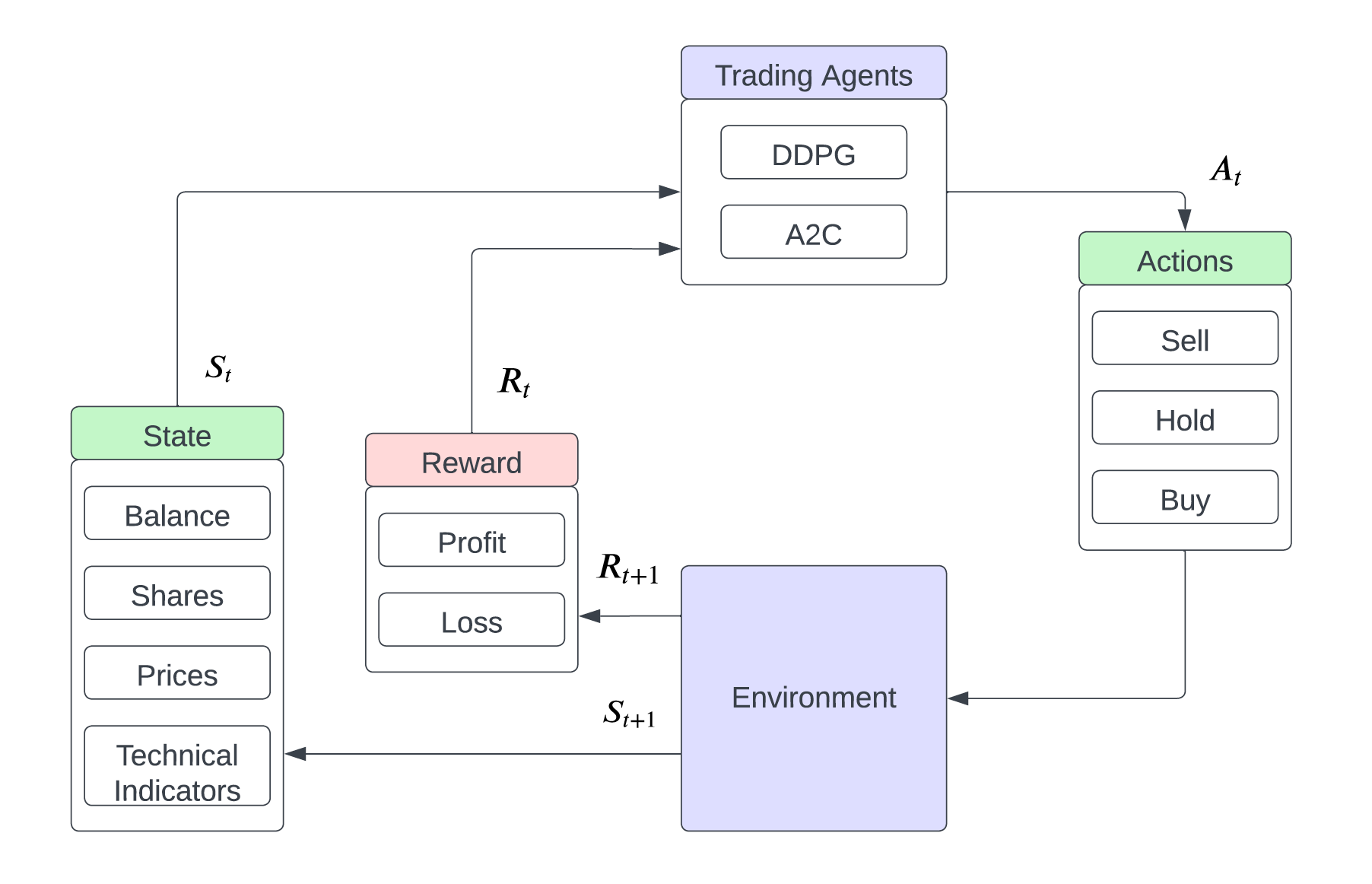
Figure 1: A General Flow Chart of FinRL Applied in Portfolio Selection

Moving-window is commonly used for time-series data, and we choose the format of 3-year training data and 1-year testing data. More specifically, the first moving window is the 06/30/2007 – 06/30/2011 data, i.e., 06/30/2007 – 06/30/2010 as the training set and 07/01/2010 – 06/30/2011 as the testing set, and other moving windows follow the same rule. We explore a total of 12 distinct moving window combinations, referred to as period 1 to period 12, wherein RL frameworks utilizing different ESG raters are constructed. Each period involves the establishment of the RL environment, determination of states and actions, and modification of reward functions as described previously. Specifically, the reward function is updated through a linear combination of the portfolio return and the weighted ESG score from each ESG rater, obtained for the corresponding period. Consequently, a comparison is conducted on the portfolio Sharpe Ratios when varying the ESG scores sourced from different raters over the same time period. The resulting Sharpe Ratio rankings of the four raters across the 12 periods spanning from 2011 to 2022 are visually presented in Figure 2.

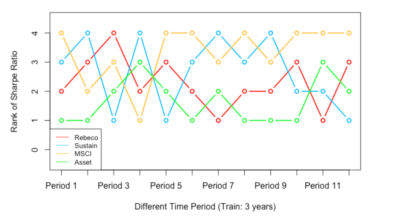
Figure 2: Ranking Comparisons

The figure shows clearly that there is no single rater that is capable of producing a portfolio that performs the best consistently over all of the 12 possible combinations of moving windows under consideration. Instead, we observed that the rankings appear to switch back and forth among the four raters for the time periods under study. This is a vivid illustration of the impacts of the wide-spread confusion among the investors for not knowing ‘with certainty’ which ESG rater to use in order to identify the best performance of the portfolios from the ranked companies. Moreover, the divergence in the ESG ratings also undermines the confidence of companies that seek to improve their ESG performances.

3 Data-Driven Ensemble Strategies

In investigating factors for the reported divergence of ESG ratings, Berg et al. (2022) decompose the ratings into three sources: (1) $53\%$ of the ranking heterogeneity can be traced back to purely measurement issues; (2) $44\%$ of the ranking disagreement is attributed to scope, where different raters include different attributes; and (3) $3\%$ of the rating differences is due to weight placed by different raters on individual components (E, S, and G) when they calculate their aggregate ESG scores for the companies. Furthermore, Berg et al. (2022) point out that there is even divergence of ratings on verifiable facts from public records. In addition, there also exists a so-called ‘rater effect’ in which a company rated highly on a particular attribute enjoys high ratings on the rest of its other attributes.

The question of interest to us is: what are the main implications of high heterogeneity in ESG rankings of companies to investors in terms of their asset allocation? It certainly does not imply that ESG ratings are so unreliable that they should not be used by investors as factors in forming their investment strategies. After all, a company’s performance in general is known to be notoriously difficult to measure with any degree of accuracy. However, it does mean that investors need to acquire a better understanding of what the ESG ratings published by different rating agencies are measuring.

Ambiguity (a.k.a. Knightian uncertainty in Economics) and risk are two related but distinct concepts in Decision Theory. Ambiguity refers to uncertainty (or lack of clarity) with unknown odds, while risk refers to the potential for loss or failure with unknown odds. Investors can have multiple views when forming their investment strategies. In general, investors’ views may vary in their level of optimism (or conservatism); as a result, these views may be associated with more or less favorable scenarios. However, it is impossible to know with certainty which views are more likely to be relatively more accurate, so investors must weigh the pros and cons of each view in order to arrive at their final decision on investment. Ambiguity refers, in particular, to the uncertainty surrounding these different views.

More specific to the context of this paper, investors are regarded to have incomplete information about ESG scores from different raters. They are not sure which one is right and what are the better weights of different ESG scores. In particular, each ESG rater can be regarded by investors as a ‘view’. Hence, confusion about ESG ratings can be regarded as a type of ambiguity. In fact, each rater has its own evaluation system. It is hard for investors to figure out which ESG rater provides a more accurate view of the ESG score and it is also not easy for investors to determine the most effective way to combine or incorporate these different views.

Instead of finding an optimal universe ESG representative in any given time period, we are going to be agnostic about it and, instead, provide several strategies to ensemble the ESG scores based on the investors’ attitudes toward ambiguity of ESG ratings by considering methods which essentially form certain weights among different ESG raters.

In particular, based on different risk and ambiguity preferences of investors, we propose data-driven criteria to identify potential distributions representing different views embraced by investors and generate ensemble strategies from these views accordingly:

1. Clustering centroid: The centroid of a group of points is a point that represents the center or average of the group. For example, in a data analysis context, the centroid of a cluster of data points might be used as a reference point to calculate the dissimilarity of each point to the centroid. For each company, we use Euclidean distance to measure a ‘dissimilarity’ between the ESG rater and the centroid. The centroid measures a minimum sum of the dissimilarity of the values in a dataset. After a trivial derivation, the centroid will reduce to the sample mean of the four raters. The centroid gives us an idea of where the ”center value” is located among the raters and this is an appropriate criterion if the investor takes all observations into consideration without losing any information. In other words, the centroid represents a decision-maker who places the same weight on those different views. However, the simple mean is known to be misleading when the data sample is skewed or contains outliers.

2. Median: The median is a measure of central tendency that is resistant to outliers or extreme values. Ambiguity-averse investors may prefer to use the median as their decision-making tool because it is a more stable and reliable measure of central tendency that is less influenced by extreme views or opinions. This can help them deal with ambiguity and make more informed investment decisions. Thus, if the ratings of the investor’s target company differ greatly among the rating agencies, the median is a more reliable metric in terms of its robustness.

3. Principal component analysis (PCA): PCA is a popular data-driven technique that is used to reduce the dimensionality of a dataset. It does this by transforming the data into a new coordinate system, in which the dimensions or variables are made to be orthogonal. The new dimensions are called principal components, and they are ordered by the amount of variation or information that they capture from the original data.

   PCA is often used to decide on a representative from a set of choices because it can help to identify the underlying structure or patterns in the data. By reducing the dimensionality of the dataset, PCA can reveal the most important variables or dimensions that capture the majority of the variation in the data. This can be useful for identifying the key factors or characteristics that are driving the variation in the data, and for selecting a representative that captures the essence of the dataset as a whole.

4. Alpha-Maxmin: Ghirardato et al. (2004) characterize the ambiguity attitude by a linear combination of the worst view and the best view, which they term as an $\alpha$ - maxmin expected utility ($\alpha$ - MEU) form,

   $$\alpha\inf_{\mathbb{Q}\in\mathcal{Q}}\mathbb{E}^{\mathbb{Q}}[U(X)]+(1-\alpha)\sup_{\mathbb{Q}\in\mathcal{Q}}\mathbb{E}^{\mathbb{Q}}[U(X)],$$ (3.1)

   where $U$ is a Bernoulli utility function, $\mathcal{Q}$ is a class of priors, $\alpha$ in $[0,1]$ is an index of ambiguity. It generalizes the $\alpha$-maxmin rule of Hurwicz to a setting of Knightian uncertainty, where a subjective perception of ambiguity is represented by a set of probability measures and the attitude toward ambiguity via the parameter $\alpha$ capturing a relative weight placed on pessimism versus optimism.

   Unlike the first three metrics, which are purely statistical and data-driven, the Alpha-Maxmin metric combines a behavioral criterion on the part of the investors with a data-driven criterion. Also, unlike the median, Alpha-Maxmin takes into account the most extreme cases among investors’ ambiguous views. This means that Alpha-Maxmin considers not just the average or typical view or opinion of investors, but also the most optimistic and most pessimistic perspectives of investors. Therefore, investors who are more concerned about the likelihood of extreme outcomes may prefer to use Alpha-Maxmin as their decision-making tool.

These four metrics are used to form ensemble strategies by combining different investment styles to create a well-rounded portfolio that meets the investor’s goals. This is acheived by incorporating investors’ ambiguous views of ESG ratings in the RL framework.

4 ESG-related Portfolio with Mean-Variance Preference

In the previous section, we have treated the heterogeneity in ESG scores generated by different ESG raters as a form of ambiguity within the realm of sustainable investments. In this section, our initial focus is on a single category of ESG scores in the presence of a general notion of uncertainty, in order to allow us to explore further the traditional linkages between risk and uncertainty studied in Finance.

We will return to the concept of ambiguity in a later stage of analysis, in particular in the empirical analysis. Our current focus is on unraveling the distinct analytical ways in which the identical ESG score type influences portfolio performance through the lens of uncertainty in general. This approach underscores our commitment to providing a nuanced and in-depth understanding of the intricate dynamics at play within the realm of sustainable investments.

To frame our discussion, we start with a general analytical framework initially. Instead of formulating investors’ preferences with an exponential utility (CARA) function as in Pástor et al. (2021) and Avramov et al. (2022), we use a mean-variance (MV) preference to formulate the utility function. Our analysis draws from Maccheroni et al. (2013), which shows the optimal investment strategy under the MV preference has an analytical closed-form expression, which provides a sharp separation for key factors of interest, such as expected return and risk. Most importantly, Maccheroni et al. (2013) also show that for a von Neumann-Morgenstern expected utility maximizing investor with a utility function $u(\cdot)$ representing investor’s attitude toward risk, and wealth $a$, who considers an investment project $h$, a linear Arrow-Pratt approximation of her certainty equivalent for an uncertain investment prospect is given by:

$$c\left(a+h,P\right)\approx a+\mathbb{E}_{P}(h)-\frac{1}{2}\gamma_{u}(a)\sigma_{P}^{2}(h))$$ (4.1)

where $c(\cdot)$ is a first-order certainty-equivalent measure and $\gamma_{u}(a)=-u^{\prime\prime}(a)/u^{\prime}(a)$ is a parameter that links risk premium and volatility. In Equation (4.1), both $\mathbb{E}_{P}(\cdot)$ and $Var_{P}(\cdot)$ are taken with respect to a particular probabilistic model (P), which describes the stochastic nature of the investment problem.

This approximation leads to an MV model with a prospect $f$ being evaluated at:

$$U(f)=\mathbb{E}(f)-\frac{\gamma_{u}(a)}{2}\sigma^{2}(f)$$ (4.2)

with $f=a+h$ and $\gamma=\gamma_{u}(a)$.

MV analysis is a crucial preliminary step in our investment strategy due to its direct relevance to the subsequent implementation of the Capital Asset Pricing Model (CAPM). By employing MV analysis, we aim to optimize the risk-return profile of our investment portfolio. MV analysis allows us to evaluate the relationship between an asset’s expected returns and its associated risk, thus enabling the identification of an efficient frontier of portfolios that offer the highest possible return for a given level of risk or the lowest possible risk for a targeted level of return. This efficient frontier forms the foundation for CAPM’s principles, as it provides a range of diversified portfolios that theoretically maximize returns based on an investor’s risk tolerance. Therefore, the judicious application of MV analysis not only refines portfolio construction but also paves the way for an extension of the Modern Portfolio Theory (MPT), proposed by Markowitz (1952), through the subsequent utilization of CAPM’s insights.

4.1 Model Setting

In principle, with additional efforts, it is possible to derive our ensuing analytical results directly from the general framework set up above. However, we do not pursue this strategy. Instead, we present a model of an ESG-related portfolio with MV preferences in the presence of general uncertainty. In a single-period economy, suppose that there is an agent who trades at time 0 and closes her position at time 1. Denote a random rate of return on the market portfolio as $\tilde{r}_{M}$, and a true and unobservable ESG score of the market portfolio as $\tilde{g}_{M}$. Let $\mu_{f}$ be a risk-free rate. We model the excess returns of the market and the ESG factor as follows.

$$Market:\quad\tilde{r}_{M}-\mu_{f}=\mu_{M}+\tilde{\epsilon}_{M},$$ (4.3)

and

$$ESG:\quad\tilde{g}_{M}=\mu_{g}+\tilde{\varepsilon}_{g,M},$$ (4.4)

where $\mathbb{E}[\tilde{r}_{M}]=\mu_{M}$ is an expected market return, $\mathbb{E}[\tilde{g}_{M}]=\mu_{g}$ is an expected value of the ESG-factor return, and $\tilde{\epsilon}_{M}$ and $\tilde{\epsilon}_{g,M}$ are zero-mean error terms, and $\sigma_{M}^{2}=\boldsymbol{X}_{M}^{T}\boldsymbol{\Sigma}_{M}\boldsymbol{X}_{M}$ and $\sigma_{g}^{2}=\boldsymbol{X}_{M}^{T}\boldsymbol{\Sigma}_{g,M}\boldsymbol{X}_{M}$ represent respectively the variance of market returns and the variance of the ESG-factor returns respectively.

Next, denote $w$ as a weight of risky assets in a portfolio, i.e. the weight of the market portfolio. The parameters $\gamma$ and $\theta$ represent the investor’s attitude toward risk associated with the market return and uncertainty associated with the ESG-factor return respectively. The objective functions for the market and the ESG factor are expressed respectively as:

$$Market\quad Objective:w\cdot\mu_{M}+(1-w)\mu_{f}-\frac{\gamma}{2}w^{2}\sigma_{M}^{2},$$ (4.5)

and

$$ESG\quad Objective:w\cdot\mu_{g}-\frac{\theta}{2}w^{2}\sigma_{g}^{2}.$$ (4.6)

The total expected utility function leads to a linear combination of the expected MV utility function of the market return and the expected MV utility function of the ESG-factor return, which gives rise to a Double-MV (DMV) model:

$$w\cdot\mu_{M}+(1-w)\mu_{f}-\frac{\gamma}{2}w^{2}\sigma_{M}^{2}+b\left(w\cdot\mu_{g}-\frac{\theta}{2}w^{2}\sigma_{g}^{2}\right),$$ (4.7)

where $b>0$ captures the relative taste of the investor between ‘pecuniary’ return and ‘non-pecuniary’ return.

Pecuniary return refers to a financial gain or loss from an investment, such as the change in the value of the investment or the income generated by the investment, such as dividends or interest. Pecuniary return is typically measured in monetary units, such as Dollars or Euros. Pecuniary return is an important consideration for investors because it represents the financial gain or loss from the investment. Investors typically want to maximize their pecuniary return in order to achieve their financial goals, such as building up wealth or generating income.

Non-pecuniary return, on the other hand, refers to non-monetary benefits or costs of an investment project, such as social, environmental, or ethical impacts of the investment. Non-pecuniary return is often referred to as ‘externalities’, as it represents the effects of the investment on parties that are not directly involved in the investment decision, which can also impact the overall performance and risk profile of the investment. For example, if a company has poor environmental practices, it may face regulatory risks or reputational damages that could negatively impact its financial performance. Similarly, if a company has poor working conditions or engages in unethical practices, it may face reputational risks or consumer backlashes that could also impact its financial performance.

Therefore, by considering both pecuniary and non-pecuniary returns in the model, we allow the investor to make informed investment decisions that take into account a full range of potential risks, uncertainties, and rewards of the investment universe. It can also help investors align their investments better with their values and ethical principles.

Next, we divide the range of $b$ into three cases:

• If $b>1$, the investors will place more emphasis on non-monetary gains.

• If $b<1$, the investors will place more emphasis on monetary gains.

• If $b=1$, the investors will be indifferent between monetary and non-monetary gains.

The optimal portfolio weights are obtained from the first-order condition of the underlying optimization program:

$$\mu_{M}-\mu_{f}-\gamma w\sigma_{M}^{2}+b\left(\mu_{g}-\theta w\sigma_{g}^{2}\right)=0$$ (4.8)

as

$$w=\frac{\mu_{M}-\mu_{f}+b\mu_{g}}{\gamma\sigma_{M}^{2}+b\theta{\sigma}_{g}^{2}}$$ (4.9)

This optimal portfolio weight can be rewritten as:

$$\frac{\mu_{M}-\mu_{f}+b\mu_{g}}{\gamma\sigma_{M}^{2}+b\theta\sigma_{g}^{2}} =\frac{\mu_{M}-\mu_{f}+b\mu_{g}}{\gamma\sigma_{M}^{2}}\cdot\frac{\gamma\sigma_{M}^{2}}{\gamma\sigma_{M}^{2}+b\theta\sigma_{g}^{2}}$$ (4.10)

$$=\left[\frac{1}{\gamma}\frac{\left(\mu_{M}-\mu_{f}\right)}{\sigma_{M}^{2}}+\frac{1}{\gamma}b\frac{\mu_{g}}{\sigma_{M}^{2}}\right]\cdot\left[1-\frac{b\theta\sigma_{g}^{2}}{\gamma\sigma_{M}^{2}+b\theta\sigma_{g}^{2}}\right]$$

$$=\frac{1}{\gamma}\frac{\left(\mu_{M}-\mu_{f}\right)}{\sigma_{M}^{2}}+\frac{1}{\gamma}b\frac{\mu_{g}}{\sigma_{M}^{2}}$$

$$-\frac{1}{\gamma}\frac{\mu_{M}-\mu_{f}+b\mu_{g}}{\sigma_{M}^{2}}\left(\frac{b\theta\sigma_{g}^{2}}{\gamma\sigma_{M}^{2}+b\theta\sigma_{g}^{2}}\right)$$

From the last line of Equation 4.10, we obtain three terms:

• First Term $\frac{1}{\gamma}\frac{\left(\mu_{M}-\mu_{f}\right)}{\sigma_{M}^{2}}$: There is no parameter in this term which involves the ESG factor, and it serves as a benchmark case of ESG indifference.

• Second Term $\frac{1}{\gamma}b\frac{\mu_{g}}{\sigma_{M}^{2}}$: This term involves the return of the ESG factor, but it does not incorporate uncertainty with respect to the ESG rating. Thus, it serves as a benchmark case with ESG preferences when the ESG profile is known with certainty.

• Last Term $\frac{1}{\gamma}\frac{\mu_{M}-\mu_{f}+b\mu_{g}}{\sigma_{M}^{2}}\left(\frac{b\theta\sigma_{g}^{2}}{\gamma\sigma_{M}^{2}+b\theta\sigma_{g}^{2}}\right)$: This term captures the incremental effect of ESG uncertainty.

Next, we define three types of investors, which have ESG indifference (I), ESG preference with no uncertainty (N), and ESG preference with uncertainty (U).

• Type-I Investors: These investors do not consider ESG factors in their decision-making processes about their decisions. They are indifferent with respect to the impacts of their investments and focus solely on their profit considerations.

• Type-N Investors: These investors prioritize ESG factors and try to align their investments with their values. However, they do not face any uncertainty associated with the ESG scores. This implies that they solely factor in the expected portfolio ESG score and do not take the ESG score’s variability into account.

• Type-U Investors: These investors also prioritize ESG factors, but they face uncertainty about the impacts of their investments on these factors. Consequently, these investors must grapple with the risk arising from variability in ESG scores. This complexity can render it more challenging for these investors to harmonize their investments with their values.

To derive a market premium, we set the first term above equal to 1 and derive the excess return of investors of type I. Similarly, letting the first two terms be 1 will lead to the formation of excess return for investors of type N. Finally, the excess return for investors of type A is derived from the original weight form $\frac{\mu_{m}-\mu_{f}+b\mu_{g,m}}{\gamma\sigma_{m}^{2}+b\theta{\sigma}_{g}^{2}}=1$. After re-arranging terms in these formulas, the excess returns of the three types of investors can be expressed as:

• Type-I Investors:

  $$\mu_{M}^{I}-\mu_{f}=\gamma\sigma_{M}^{2}$$ (4.11)

• Type-N Investors:

  $$\mu_{M}^{N}-\mu_{f}=\gamma\sigma_{M}{}^{2}-b\mu_{g}$$ (4.12)

• Type-U Investors:

  $$\mu_{M}^{U}-\mu_{f}=\gamma\sigma_{M}^{2}+b\theta\sigma_{g}^{2}-b\mu_{g}$$ (4.13)

Hence, the differences in expected returns between these three types of investors are given:

$$\mu_{M}^{N}-\mu_{M}^{I}=-b\mu_{g}<0$$ (4.14)

$$\mu_{M}^{U}-\mu_{M}^{N}=b\theta\sigma_{g}^{2}>0$$ (4.15)

$$\mu_{M}^{U}-\mu_{M}^{I}=b\theta\sigma_{g}^{2}-b\mu_{g,M}=b(\theta\sigma_{g}^{2}-\mu_{g})$$ (4.16)

If we assume that $b>0$, then the no-uncertainty case is associated with a negative ESG incremental premium. Pástor et al. (2021) pointed out that sustainable investing produces a positive social impact by making firms greener and by shifting real investment toward green firms. In order to achieve the gains from ESG, investors are willing to sacrifice their returns. Green assets have low expected returns because investors enjoy holding them and also because green assets hedge climate risk.

In addition, it is evident from the second equation that the market premium increases with ESG uncertainty. The uncertainty of ESG scores contributes to additional risk for investors; so the required return should reflect the corresponding compensation for higher uncertainty. However, the sign of the incremental premium is indeterminate when we compare the ESG indifference case and the ESG preference with uncertainty case due to the conflicting forces emanating from the variance and return of the ESG scores. This can be explained as follows: the investors who prefer non-monetary returns with ESG uncertainty will get compensation from the risks of the ESG uncertainty as well as take the loss from the non-monetary return.

Next, we derive the portfolio variances for these three types of investors:

$$\sigma_{M}^{N}-\sigma_{M}^{I}=\frac{2\left(\mu_{M}-\mu_{f}\right)b\mu_{g}+b^{2}\mu_{g}^{2}}{\gamma^{2}\sigma_{M}^{2}}>0,$$ (4.17)

and

$$\sigma_{M}^{U}-\sigma_{M}^{N}=\frac{\left(\mu_{M}-\mu_{f}+b\mu_{g}\right)^{2}}{\gamma^{2}\sigma_{M}{}^{2}}\cdot\left[\frac{-2\gamma\sigma_{M}^{2}b\theta\sigma_{g}{}^{2}-b^{2}\theta^{2}\sigma_{g}^{4}}{\left(\gamma\sigma_{M}^{2}+b\theta\sigma_{g}^{2}\right)^{2}}\right]<0,$$ (4.18)

and

$$\sigma_{M}^{U}-\sigma_{M}^{I}=\frac{\left(\mu_{M}-\mu_{f}\right)^{2}\left[E_{g}-1\right]+\left[2\left(\mu_{M}-\mu\right)b\mu_{g}+b^{2}\mu_{g}^{2}\right]E_{g}}{\gamma^{2}\sigma_{M}{}^{2}},$$ (4.19)

where $E_{g}=\frac{\left(\gamma\sigma_{M}^{2}\right)^{2}}{\left(\gamma\sigma_{M}^{2}+b\theta{\sigma}_{g}^{2}\right)^{2}}\in(0,1)$, which can be interpreted as a ratio of the risk of market returns to the overall risk after taking into account the degree of aversion.

The variance relationships between different investors are generally the reverse of the return relationships, with the exception of the indeterminate relationship between the ESG indifference case and the ESG preference with uncertainty case.

Thus, it is reasonable to expect the returns, variances, and Sharpe ratios for these three types of investors to have the following ex-ante relationships between the different types of investors (see Table  2).

	Return	Variance	Sharpe Ratio
ESG Indifference	Large	Small	Large
Without Uncertainty	Small	Large	Small
With ESG Uncertainty	Around Large	Around Small	Around Large

Table 2: Ex-ante Relationships between Different Types of Investors

It is also noted that, with a slight abuse of notation, we use the phrase of ‘Around Large/Around Small’ in this table. For example, it suggests that for investors with ESG uncertainty, it is unclear which group will receive higher returns compared to ESG indifferent investors, and this is referred to as ‘Around Large.’

4.2 Calibration Exercise

To assess the alignment between theoretical models and real-world portfolio selection outcomes, we conduct the following calibration exercises using the RL framework.

Data Source: The study utilizes a dataset covering the period from 06/30/2018 to 06/30/2021 for the training set and 07/01/2021 to 06/30/2022 for the testing set. In each calibration, we choose to use ESG data from the four major ESG raters separately. In addition, the four kinds of proposed ensemble ESG scores in Section 3 present an alternative ESG feature option for investors, and consequently, we conduct calibration exercises by incorporating the four suggested ensemble scores individually. This exploration allows us to comprehensively assess the viability and potential impact of these ensemble scores within our analytical framework. By considering these ensemble scores alongside individual ESG metrics, we endeavor to provide investors with a more nuanced understanding of their investment choices and their alignment with sustainable practices.

RL Framework: We maintain the configuration of the RL framework in accordance with the FinRL framework, as elaborated in Section 2. Our framework continues to comprise three distinct layers. Within the Agent layer, we still utilize the DDPG algorithm as the central agent for our FinRL-based investigations. In the bottom layer, the environment layer, we persist in simulating authentic financial markets, relying on historical data that encompasses various metrics, including closing prices, stock quantities, trading volume, and technical indicators.

Within the application layer, we integrate an algorithmic trading strategy into the RL framework by defining the state space, action space, and reward function. The state space remains inclusive of information such as account balance, current asset holdings, Open-High-Low-Close (OHLC) prices, trading volume, and technical indicators. The action space outlines the allowable actions through which the agent engages with the environment. Typically, an action ’a’ is composed of three components: -1, 0, 1, where -1, 0, and 1 correspond to selling, holding, and purchasing one share, respectively. In terms of the reward function modification, the study explicitly incorporates the MV preference as a distinct reward function in the RL framework. This modified reward function is subsequently trained separately for the three types of investors specified. To be specific, the reward function for each type of investor is set as:

• Type-I Investors:

  $$w\cdot\mu_{M}+(1-w)\mu_{f}-\frac{\gamma}{2}w^{2}\sigma_{M}^{2}$$ (4.20)

• Type-N Investors:

  $$w\cdot\mu_{M}+(1-w)\mu_{f}-\frac{\gamma}{2}w^{2}\sigma_{M}^{2}+bw\cdot\mu_{g}$$ (4.21)

• Type-U Investors:

  $$w\cdot\mu_{M}+(1-w)\mu_{f}-\frac{\gamma}{2}w^{2}\sigma_{M}^{2}+b\left(w\cdot\mu_{g}-\frac{\theta}{2}w^{2}\sigma_{g}^{2}\right)$$ (4.22)

After constructing the layers, we proceed to train the process using FinRL for each calibration iteration. This training involves monitoring price fluctuations, making decisions (such as selling, holding, or buying a specific quantity of stock), and determining rewards based on various investor profiles. The outcomes generated by the models, utilizing ESG scores sourced from four individual ESG raters and four ensemble methods, are presented in Table 3 and Table 4 below. The RL framework’s configuration remains consistent across the creation of these two tables, with the only variation being the source of ESG scores or the ensemble methods applied. Both tables display the calibration results for three distinct investor types.

	$b<1(b=0.2)$		$b<1(b=0.6)$		$b=1$		$b>1(b=1.4)$		$b>1(b=1.8)$
	Return	SR	Return	SR	Return	SR	Return	SR	Return	SR
ESG Indifference	$8.63\%$	0.77	$8.63\%$	0.77	$8.63\%$	0.77	$8.63\%$	0.77	$8.63\%$	0.77
RebecoSAM (N)	$9.52\%$	0.78	$8.01\%$	0.70	$7.99\%$	0.66	$7.93\%$	0.65	$7.25\%$	0.53
Sustain (N)	$7.66\%$	0.63	$7.63\%$	0.66	$7.68\%$	0.60	$7.63\%$	0.58	$7.45\%$	0.54
MSCI (N)	$8.04\%$	0.72	$7.89\%$	0.69	$7.21\%$	0.58	$6.26\%$	0.53	$7.00\%$	0.52
Asset4 (N)	$9.64\%$	0.81	$8.21\%$	0.72	$8.23\%$	0.70	$8.03\%$	0.67	$7.45\%$	0.55
RebecoSAM (U)	$9.56\%$	0.77	$8.45\%$	0.74	$7.61\%$	0.68	$8.31\%$	0.72	$7.38\%$	0.47
Sustain (U)	$9.61\%$	0.80	$8.78\%$	0.81	$8.54\%$	0.77	$7.73\%$	0.62	$7.51\%$	0.53
MSCI (U)	$9.99\%$	0.88	$8.42\%$	0.74	$7.87\%$	0.69	$7.62\%$	0.62	$7.40\%$	0.58
Asset4 (U)	$9.23\%$	0.84	$8.63\%$	0.75	$8.33\%$	0.72	$8.23\%$	0.64	$7.33\%$	0.48

Table 3: Calibration Results for Four Individual ESG Raters

	$b<1(b=0.2)$		$b<1(b=0.6)$		$b=1$		$b>1(b=1.4)$		$b>1(b=1.8)$
	Return	SR	Return	SR	Return	SR	Return	SR	Return	SR
ESG Indifference	$8.63\%$	0.77	$8.63\%$	0.77	$8.63\%$	0.77	$8.63\%$	0.77	$8.63\%$	0.77
Centroid (N)	$8.45\%$	0.68	$8.12\%$	0.65	$7.38\%$	0.64	$7.05\%$	0.64	$6.68\%$	0.60
Median (N)	$7.66\%$	0.63	$7.63\%$	0.66	$7.68\%$	0.62	$7.63\%$	0.64	$7.45\%$	0.63
PCA (N)	$8.04\%$	0.72	$7.89\%$	0.69	$7.21\%$	0.66	$6.26\%$	0.63	$7.00\%$	0.62
Alpha-Maxmin (N)	$9.03\%$	0.74	$8.34\%$	0.70	$8.12\%$	0.68	$7.88\%$	0.65	$7.43\%$	0.63
Centroid (U)	$9.29\%$	0.73	$8.62\%$	0.69	$8.03\%$	0.64	$7.68\%$	0.59	$7.12\%$	0.53
Median (U)	$9.61\%$	0.80	$8.78\%$	0.81	$8.54\%$	0.77	$7.73\%$	0.62	$7.51\%$	0.53
PCA (U)	$9.23\%$	0.84	$8.63\%$	0.75	$8.33\%$	0.72	$8.23\%$	0.64	$7.33\%$	0.48
Alpha-Maxmin (U)	$9.99\%$	0.88	$8.72\%$	0.78	$8.63\%$	0.72	7.62%	0.62	$7.40\%$	0.58

Table 4: Calibration Results for Four Ensemble ESG Scores

The results presented in Table 3 and Table 4 can be summarized as follows. In scenarios devoid of uncertainty, investors exhibiting indifference towards ESG factors typically achieve higher expected returns compared to those who prioritize ESG considerations. Conversely, investors who account for ESG uncertainty tend to realize higher expected returns than their counterparts who do not factor in such uncertainties. It is noteworthy, however, that the expected returns and corresponding Sharpe ratios of investors with ESG uncertainty do not consistently surpass those of ESG-indifferent investors. Moreover, an increase in the parameter $b$ corresponds to a heightened emphasis on non-pecuniary returns, ultimately resulting in lower overall expected returns. Interestingly, the highest expected returns and Sharpe ratios are often attained by investors displaying indifference towards ESG factors or those considering ESG uncertainty. Notably, among the ensemble ESG score methodologies, Alpha-Maxmin consistently demonstrates superior performance in terms of expected portfolio return and Sharpe ratio when compared to other ensemble methods.

The results presented above are broadly in agreement with the theoretical expectations of the model. However, there are a few isolated instances, in which the empirical results deviate from the theoretical predictions. Such deviations may arise due to a number of reasons, such as overfitting the model, a limited amount of the data used for training the model, etc.

5 ESG-Modified Capital Asset Pricing Model

For completeness of our analysis, we extend a Capital Asset Pricing Model (CAPM) introduced by Sharpe (1964) to include the ESG scores and also by accounting for uncertainty by leveraging the results obtained earlier for the MV model.

Firstly, we provide a list of variable declarations in Table 5.

Variable	Description	Dimension
$\boldsymbol{X}_{i}$	Agent $i$’s portfolio weights for $n$ stocks	$n\times 1$ vector
$\boldsymbol{X}_{M}$	Market portfolio vector	$n\times 1$ vector
$\boldsymbol{\mu}_{r}$	Market excess return vector	$n\times 1$ vector
${\mu}_{M}=\boldsymbol{X}_{M}^{T}\boldsymbol{\mu}_{r}$	Market expected return	A number
$\boldsymbol{\mu}_{g,M}$	Expected ESG score vector	$n\times 1$ vector
${\mu}_{g}=\boldsymbol{X}_{M}^{T}\boldsymbol{\mu}_{g,M}$	Market ESG score	A number
$\boldsymbol{\Sigma}_{M}$	Covariance matrix of returns	$n\times n$ matrix
$\boldsymbol{\Sigma}_{g,M}$	Covariance matrix of ESG ratings	$n\times n$ matrix
$w_{i}$	Weight of Agent $i$	A number
$\sigma_{M}^{2}=\boldsymbol{X}_{M}^{T}\boldsymbol{\Sigma}_{M}\boldsymbol{X}_{M}$	Market return variance	A number
$\sigma_{g}^{2}=\boldsymbol{X}_{M}^{T}\boldsymbol{\Sigma}_{g,M}\boldsymbol{X}_{M}$	Market ESG score variance	A number

Table 5: Description of Variables

The direct utility function for investor $i$ is formulated as:

$$\boldsymbol{X}_{i}^{T}\boldsymbol{\mu}_{r}-\frac{\gamma_{i}}{2}\boldsymbol{X}_{i}^{T}\boldsymbol{\Sigma}_{M}\boldsymbol{X}_{i}+b_{i}\left(\boldsymbol{X}_{i}^{T}\boldsymbol{\mu}_{g,M}-\frac{\theta_{i}}{2}\boldsymbol{X}_{i}^{T}\boldsymbol{\Sigma}_{g,M}\boldsymbol{X}_{i}\right)$$ (5.1)

After taking the first-order condition, the agent $i$’s portfolio weights for $n$ stocks can be expressed as:

$$\boldsymbol{X}_{i} =\left(\gamma_{i}\boldsymbol{\Sigma}_{M}+b_{i}\theta_{i}\boldsymbol{\Sigma}_{g,M}\right)^{-1}\left(\boldsymbol{\mu}_{r}+b_{i}\boldsymbol{\mu}_{g,M}\right)$$

$$=\left(\gamma_{i}\boldsymbol{\Sigma}_{M}+b_{i}\theta_{i}\boldsymbol{\Sigma}_{g,M}\right)^{-1}\cdot\gamma_{i}\boldsymbol{\Sigma}_{M}\left(\frac{1}{\gamma_{i}}\boldsymbol{\Sigma}_{M}{}^{-1}\right)\cdot\left(\boldsymbol{\mu}_{r}+b_{i}\boldsymbol{\mu}_{g,M}\right)$$

$$=\left(\gamma_{i}\boldsymbol{\Sigma}_{M}+b_{i}\theta_{i}\boldsymbol{\Sigma}_{g,M}\right)^{-1}\cdot\gamma_{i}\boldsymbol{\Sigma}_{M}\cdot\frac{1}{\gamma_{i}}\left[\boldsymbol{\Sigma}_{M}^{-1}\left(\boldsymbol{\mu}_{r}\right)+\boldsymbol{\Sigma}_{M}{}^{-1}b_{i}\boldsymbol{\mu}_{g,M}\right]$$

$$={\left[\frac{1}{\gamma_{i}}\boldsymbol{\Sigma}_{M}^{-1}\left(\boldsymbol{\mu}_{r}\right)+\frac{1}{\gamma_{i}}\boldsymbol{\Sigma}_{M}{}^{-1}b_{i}\boldsymbol{\mu}_{g,M}\right]}$$

$$-{\left[\left(\gamma_{i}\boldsymbol{\Sigma}_{M}+b_{i}\theta_{i}\boldsymbol{\Sigma}_{g,M}\right)^{-1}\cdot b_{i}\theta_{i}\boldsymbol{\Sigma}_{g,M}\right]{\left[\frac{1}{\gamma_{i}}\boldsymbol{\Sigma}_{M}^{-1}\left(\boldsymbol{\mu}_{r}\right)+\frac{1}{\gamma_{i}}\boldsymbol{\Sigma}_{M}{}^{-1}b_{i}\boldsymbol{\mu}_{g,M}\right]}}$$ (5.2)

5.1 ESG-Modified CAPM without Uncertainty

In the absence of ESG uncertainty, we only take the first two terms of Equation  5.2 into consideration, and as a result, the market portfolio is given by:

$$\boldsymbol{X}_{M}=\sum_{i=1}^{I}w_{i}\left[\frac{1}{\gamma_{i}}\boldsymbol{\Sigma}_{M}^{-1}\left(\boldsymbol{\mu}_{r}\right)+\frac{1}{\gamma_{i}}b_{i}\cdot\boldsymbol{\Sigma}_{M}{}^{-1}\cdot\boldsymbol{\mu}_{g,M}\right]$$ (5.3)

Then,

$$\boldsymbol{\Sigma}_{M}\boldsymbol{X}_{M}=\sum_{i=1}^{I}\frac{w_{i}}{\gamma_{i}}\cdot\boldsymbol{\mu}_{r}+\sum_{i=1}^{I}\frac{w_{i}}{\gamma_{i}}\cdot b_{i}\cdot\boldsymbol{\mu}_{g,M}$$ (5.4)

Let $\gamma_{M}=\frac{1}{\sum_{i=1}^{I}w_{i}\cdot\frac{1}{\gamma_{i}}}$ and $b_{M}=\frac{\sum_{i=1}^{I}w_{i}\cdot\frac{b_{i}}{\gamma_{i}}}{\sum_{i=1}^{I}w_{i}\cdot\frac{1}{\gamma_{i}}}=\left(\sum_{i=1}^{I}w_{i}\cdot\frac{b_{i}}{\gamma_{i}}\right)\cdot\gamma_{M}$, then

$$\boldsymbol{\Sigma}_{M}\boldsymbol{X}_{M}=\frac{1}{\gamma_{M}}\cdot\boldsymbol{\mu}_{r}+\frac{b_{M}}{\gamma_{M}}\cdot\boldsymbol{\mu}_{g,M},$$ (5.5)

$$\boldsymbol{\mu}_{r} =\gamma_{m}\boldsymbol{\Sigma}_{M}\boldsymbol{X}_{M}-b_{M}\cdot\boldsymbol{\mu}_{g,M}$$ (5.6)

$$=\frac{\boldsymbol{\Sigma}_{M}\boldsymbol{X}_{M}}{\sigma_{M}^{2}}\cdot\gamma_{M}\sigma_{M}^{2}-b_{M}\cdot\boldsymbol{\mu}_{g,M}$$

Next, we derive the market expected return ${\mu}_{M}$ by multiplying $\boldsymbol{X}_{M}^{T}$ on both sides of Equation  5.6.

$$\mu_{M}=\boldsymbol{X}_{M}^{T}\boldsymbol{\mu}_{r}=\gamma_{M}\boldsymbol{X}_{M}^{T}\boldsymbol{\Sigma}_{M}\boldsymbol{X}_{M}-\boldsymbol{X}_{M}^{T}\left(b_{M}\cdot\boldsymbol{\mu}_{g,M}\right)=\gamma_{M}\sigma_{M}^{2}-\boldsymbol{X}_{M}^{T}\left(b_{M}\cdot\boldsymbol{\mu}_{g,M}\right)$$ (5.7)

From Equation  5.7, we know $\gamma_{M}\sigma_{M}^{2}=\mu_{M}+\boldsymbol{X}_{M}^{T}\left(b_{M}\cdot\boldsymbol{\mu}_{g,M}\right)$. Then, we replace $\gamma_{M}\sigma_{M}^{2}$ by $\mu_{M}+\boldsymbol{X}_{M}^{T}\left(b_{M}\cdot\boldsymbol{\mu}_{g,M}\right)$ in Equation  5.6.

After re-arranging terms, an ESG-modified CAPM without uncertainty is shown in Equation  5.8, where $\boldsymbol{\beta}=\frac{\boldsymbol{\Sigma}_{M}\boldsymbol{X}_{M}}{\sigma_{M}^{2}}$. Here, Alpha ($\boldsymbol{\alpha}$) can be expressed as $b_{M}\left(\boldsymbol{\beta}\mu_{g}-\boldsymbol{\mu}_{g,M}\right)$.

$$\boldsymbol{\mu}_{r} =\frac{\boldsymbol{\Sigma}_{M}\boldsymbol{X}_{M}}{\sigma_{M}^{2}}\cdot\mu_{M}+\frac{\boldsymbol{\Sigma}_{M}\boldsymbol{X}_{M}}{\sigma_{M}^{2}}\boldsymbol{X}_{M}{}^{T}\cdot b_{M}\cdot\boldsymbol{\mu}_{g,M}-b_{M}\cdot\boldsymbol{\mu}_{g,M}$$ (5.8)

$$=\boldsymbol{\beta}\mu_{M}+b_{M}\left[\boldsymbol{\beta}\mu_{g}-\boldsymbol{\mu}_{g,M}\right]$$

The expected excess return of investors is affected by two factors, which are a modified market premium (purely market features $\boldsymbol{\beta}\mu_{M}$) as well as an Alpha component (features related to ESG scores $b_{M}\left[\boldsymbol{\beta}\mu_{g}-\boldsymbol{\mu}_{g,M}\right]$). The alpha value, which represents excess returns not explained by the stock’s beta and the market return, is influenced by the difference between a company’s own ESG score and the market ESG score, multiplied by the stock’s beta.

To illustrate this concept numerically, consider a stock with a beta of 1.5 and a market ESG score of 2. If the stock’s own ESG score is 2.5, it will have a positive alpha ($+0.5$). On the other hand, if the ESG score is greater than 3.0, the alpha will be negative. This also coincides with the previous conclusion: after considering the preference for the ESG factor, the expected return will decrease. A higher ESG requirement will lead to a greater loss of expected return.

5.2 ESG-Modified CAPM with Uncertainty

For the case with ESG uncertainty, the market portfolio is given by:

$$\boldsymbol{X}_{M} =\sum_{i=1}^{I}w_{i}\cdot\boldsymbol{X}_{i}$$ (5.9)

$$=\sum_{i=1}^{I}w_{i}\cdot\left(\gamma_{i}\boldsymbol{\Sigma}_{M}+b_{i}\theta_{i}\boldsymbol{\Sigma}_{g,M}\right)^{-1}\cdot\boldsymbol{\Sigma}_{M}^{-1}\left(\boldsymbol{\mu}_{r}+b_{i}\boldsymbol{\mu}_{g,M}\right)$$

$$\boldsymbol{\Sigma}_{M}\boldsymbol{X}_{M} =\sum_{i=1}^{I}w_{i}\left(\gamma_{i}\boldsymbol{\Sigma}_{M}+b_{i}\theta_{i}\boldsymbol{\Sigma}_{g,M}\right)^{-1}\left(\boldsymbol{\mu}_{r}+b_{i}\boldsymbol{\mu}_{g,M}\right)$$ (5.10)

$$=\sum_{i=1}^{I}w_{i}\left(\gamma_{i}\boldsymbol{\Sigma}_{M}+b_{i}\theta_{i}\boldsymbol{\Sigma}_{g,M}\right)^{-1}\boldsymbol{\mu}_{r}+\sum_{i=1}^{I}w_{i}\left(\gamma_{i}\boldsymbol{\Sigma}_{M}+b_{i}\theta_{i}\boldsymbol{\Sigma}_{g,M}\right)^{-1}b_{i}\cdot\boldsymbol{\mu}_{g,M}$$

$$={\boldsymbol{\Gamma}_{M,U}}^{-1}\cdot\boldsymbol{\mu}_{r}+{\boldsymbol{B}_{M,U}}{\boldsymbol{\Gamma}_{M,U}}^{-1}\cdot\boldsymbol{\mu}_{g,M}$$

where $\boldsymbol{\Gamma}_{M,U}={\left(\sum_{i=1}^{I}w_{i}\left(\gamma_{i}\boldsymbol{\Sigma}_{M}+b_{i}\theta_{i}\boldsymbol{\Sigma}_{g,M}\right)^{-1}\right)}^{-1}$, and

$$\boldsymbol{B}_{M,U} ={\left(\sum_{i=1}^{I}w_{i}\left(\gamma_{i}\boldsymbol{\Sigma}_{M}+b_{i}\theta_{i}\boldsymbol{\Sigma}_{g,M}\right)^{-1}b_{i}\right)}\cdot{\left(\sum_{i=1}^{I}w_{i}\left(\gamma_{i}\boldsymbol{\Sigma}_{M}+b_{i}\theta_{i}\boldsymbol{\Sigma}_{g,M}\right)^{-1}\right)}^{-1}$$ (5.11)

$$=\boldsymbol{\Gamma}_{M,U}\left(\sum_{i=1}^{I}w_{i}\left(\gamma_{i}\boldsymbol{\Sigma}_{M}+b_{i}\theta_{i}\boldsymbol{\Sigma}_{g,M}\right)^{-1}b_{i}\right).$$

Equation  5.10 has the same form as Equation  5.5. The following derivation process should be the same as the case without ESG uncertainty. Thus, the CAPM for Type-U investors is given by:

$$\boldsymbol{\mu}_{r} =\frac{\boldsymbol{\Sigma}_{M}\boldsymbol{X}_{M}}{\sigma_{M}^{2}}\cdot\mu_{M}+\frac{\boldsymbol{\Sigma}_{M}\boldsymbol{X}_{M}}{\sigma_{M}^{2}}\boldsymbol{X}_{M}{}^{T}\cdot\boldsymbol{B}_{M,U}\cdot\boldsymbol{\mu}_{g,M}-\boldsymbol{B}_{M,U}\cdot\boldsymbol{\mu}_{g,M}$$ (5.12)

$$=\boldsymbol{\beta}\mu_{M}+\boldsymbol{B}_{M,U}\left(\boldsymbol{\beta}\mu_{g}-\boldsymbol{\mu}_{g,M}\right),$$

where $\boldsymbol{\beta}=\frac{\boldsymbol{\Sigma}_{M}\boldsymbol{X}_{M}}{\sigma_{M}^{2}}$ and the Alpha ($\boldsymbol{\alpha}$) can be expressed as $\boldsymbol{B}_{M,U}\left(\boldsymbol{\beta}\mu_{g}-\boldsymbol{\mu}_{g,M}\right)$.

The final form for Type-U investors is the same as the case for the type-N investors, except that the $\boldsymbol{B}_{M,U}$ is defined with the incorporation of $\boldsymbol{\Sigma}_{g,M}$ to express the features of ESG Uncertainty. Similarly, when dealing with situations that encompass uncertainty, the Alpha-value retains its sensitivity to the disparity between a company’s specific ESG score and the market’s ESG score, multiplied by the stock’s beta. Employing the same example as previously demonstrated, envision a stock with a beta of 1.5 and a market ESG score of 2. In this context, if the stock’s individual ESG score remains at 2.5, a positive alpha ($+0.5$) will be generated. Conversely, should the ESG score exceed 3.0, the resultant alpha will shift to a negative value.

In principle, a full calibration exercise can be carried out to illustrate the efficacy of the ESG-modified CAPM with and without uncertainty and the results can then be compared with those obtained from the traditional CAPM. This is left for a future study.

6 Conclusions

Modern investors prioritize ESG scores, aligning their investments with companies that champion environmental responsibility, social awareness, and robust governance. The landscape of ESG data providers is diversified and encompasses well-established players. The existing literature tends to focus on the beneficial role of ESG integration in generating expected excess returns or risk premia.

With the abundance of variety comes heterogeneity. It is not uncommon for the rating agencies to disagree with their published ESG ratings for companies in their samples. This divergence in the ESG ratings affects both the investors, who wish to achieve the financial and ESG-factor return objectives, and the companies, who seek to improve their ESG performances.

The heterogeneity of ESG ratings by major rating agencies is treated in this paper as a source of ambiguity. In response to this view, firstly we have proposed four ESG ensemble strategies that cater to different risk and ambiguity preference profiles, instead of providing only a single, optimal ESG scoring system.

In our portfolio optimization strategy in Section 2, we incorporate the ESG scores explicitly in the reward function of the RL model to analyze the effect of widespread confusion caused by the heterogeneity in the ESG ratings on the coherence of investment strategies.

Second, to combine the goals of achieving both the financial and ESG-factor return objectives, we present a Double-MV (DMV) model, which is a linear combination of the two objectives with a preference ratio parameter. In this model, we define three types of investors: those who are indifferent to ESG, those who prefer ESG but are not affected by uncertainty with respect to the ESG ratings, and those who prefer ESG and are affected by uncertainty with respect to the ESG ratings. Our analysis of the optimal portfolio weights for these investors can be summarized as follows: (i) the no-uncertainty case is associated with a negative ESG incremental premium; (ii) uncertainty with respect to the ESG ratings increases the risk for the investors, and the required return reflects this added risk; and (iii) the sign of the incremental premium is indeterminate when comparing the ESG indifference case and the ESG preference with uncertainty case due to conflicting forces at work between the risk and the return of the ESG factor.

Additionally, the relationships for the variances of the investors are in reverse to those for the expected mean relationships. When incorporating the ESG ratings with uncertainty in the model, its variance is larger than that without incorporating the ESG ratings. When incorporating the uncertain ESG ratings, its variance is smaller than that for the case without uncertainty. However, the difference between the ESG indifference case and the ESG preference with uncertainty case is indeterminate. In order to verify the practicality of the proposed theoretical model, we use an RL model by setting the reward function to be the specified DMV model.

Third, to complete our analysis, we leverage the results obtained for the DMV model to construct ESG-modified CAPMs for ESG preference investors with and without uncertainty with respect to the ESG ratings, in order to evaluate the performance of the resulting optimized portfolio. Both models are shown to have a similar structure and divide the expected return into two components, which are the modified market premium (based on pure market factors) and the Alpha component (based on the ESG factor). Our analysis shows that the Alpha value is affected by the difference between a company’s individual ESG ratings and the market ESG ratings, multiplied by the stock’s beta. This information can be used to determine a threshold for positive Alpha in a sustainable investment approach, aiming to shed light on these intricacies, and guiding both investors and companies towards more informed, sustainable choices.

References

- Avramov et al. (2022) Avramov, D., Cheng, S., Lioui, A., Tarelli, A., 2022. Sustainable investing with ESG rating uncertainty. Journal of Financial Economics 145, 642–664.
- Berg et al. (2022) Berg, F., Koelbel, J.F., Rigobon, R., 2022. Aggregate confusion: The divergence of ESG ratings. Review of Finance 26, 1315–1344.
- Ghirardato et al. (2004) Ghirardato, P., Maccheroni, F., Marinacci, M., 2004. Differentiating ambiguity and ambiguity attitude. Journal of Economic Theory 118, 133–173.
- Jiang et al. (2017) Jiang, Z., Xu, D., Liang, J., 2017. A deep reinforcement learning framework for the financial portfolio management problem. arXiv preprint arXiv:1706.10059 .
- Kaelbling et al. (1996) Kaelbling, L.P., Littman, M.L., Moore, A.W., 1996. Reinforcement learning: A survey. Journal of Artificial Intelligence Research 4, 237–285.
- Li et al. (2021) Li, Z., Liu, X.Y., Zheng, J., Wang, Z., Walid, A., Guo, J., 2021. Finrl-podracer: High performance and scalable deep reinforcement learning for quantitative finance, in: Proceedings of the Second ACM International Conference on AI in Finance, pp. 1–9.
- Liu et al. (2020) Liu, X.Y., Yang, H., Chen, Q., Zhang, R., Yang, L., Xiao, B., Wang, C.D., 2020. Finrl: A deep reinforcement learning library for automated stock trading in quantitative finance. arXiv preprint arXiv:2011.09607 .
- Maccheroni et al. (2013) Maccheroni, F., Marinacci, M., Ruffino, D., 2013. Alpha as ambiguity: Robust mean-variance portfolio analysis. Econometrica 81, 1075–1113.
- Maree and Omlin (2022) Maree, C., Omlin, C.W., 2022. Balancing profit, risk, and sustainability for portfolio management, in: 2022 IEEE Symposium on Computational Intelligence for Financial Engineering and Economics (CIFEr), IEEE. pp. 1–8.
- Markowitz (1952) Markowitz, H., 1952. Portfolio selection. The Journal of Finance 7, 77–91.
- Pástor et al. (2021) Pástor, L., Stambaugh, R.F., Taylor, L.A., 2021. Sustainable investing in equilibrium. Journal of Financial Economics 142, 550–571.
- Sharpe (1964) Sharpe, W.F., 1964. Capital asset prices: A theory of market equilibrium under conditions of risk. The Journal of Finance 19, 425–442.
- Sutton and Barto (2018) Sutton, R.S., Barto, A.G., 2018. Reinforcement learning: An introduction. MIT press.
- Vo et al. (2019) Vo, N.N., He, X., Liu, S., Xu, G., 2019. Deep learning for decision making and the optimization of socially responsible investments and portfolio. Decision Support Systems 124, 113097.