Fast algorithm for centralized multi-agent maze exploration

Abstract

Recent advancements in robotics have paved the way for robots to replace humans in perilous situations, such as searching for victims in blazing buildings, earthquake-damaged structures, uncharted caves, traversing minefields, or patrolling crime-ridden streets. These challenges can be generalized as problems where agents need to explore unknown mazes. Although various algorithms for single-agent maze exploration exist, extending them to multi-agent systems poses complexities.

We propose a solution: a cooperative multi-agent system of automated mobile agents for exploring unknown mazes and locating stationary targets. Our algorithm employs a potential field governing maze exploration, integrating cooperative agent behaviors like collision avoidance, coverage coordination, and path planning.

This approach builds upon the Heat Equation Driven Area Coverage (HEDAC) method by Ivić, Crnković, and Mezić. Unlike previous continuous domain applications, we adapt HEDAC for discrete domains, specifically mazes divided into nodes. Our algorithm is versatile, easily modified for anti-collision requirements, and adaptable to expanding mazes and numerical meshes over time.

Comparative evaluations against alternative maze-solving methods illustrate our algorithm’s superiority. The results highlight significant enhancements, showcasing its applicability across diverse mazes. Numerical simulations affirm its robustness, adaptability, scalability, and simplicity, enabling centralized parallel computation in autonomous systems of basic agents/robots.

[mathri]organization=Faculty of Mathematics, University of Rijeka, addressline=Radmile Matejčić 2, city=Rijeka, postcode=51000, country=Croatia [uniri]organization=Faculty of Engineering, University of Rijeka, addressline=Vukovarska 58, city=Rijeka, postcode=51000, country=Croatia [unimostar]organization=Faculty of Science and Education, University of Mostar, addressline=Matice hrvatske bb, city=Mostar, postcode=88000, country=Bosnia and Herzegovina

1 Introduction

Maze exploration has captured human curiosity for an extended period. It has served as a valuable tool in scientific investigations, frequently assessing the cognitive skills of animals, notably mice, and more recently, examining the artificial intelligence competencies of robots. Algorithms for maze exploration by a single agent are commonly used to solve mazes, but their extensions to multi-agent systems are not optimal which leaves room for improvement.

When the maze’s layout, including its walls and corridors, is already known, agents typically rely on path-planning algorithms to navigate through the maze, ultimately reaching their goal, such as an exit. However, in cases where the maze is unknown in advance, agents must initially explore the immediate surroundings using sensors and then strategize their actions based on the gathered information. Consequently, the challenge of navigating an unknown maze in search of stationary targets, like an exit, encompasses problems related to sensing, searching, and path-finding, and can be tackled using correspondent methods and techniques.

In this work, we consider the problem of exploration of an unknown maze by a cooperative multi-agent system that traverses the maze along continuous paths in discrete time. Every maze is defined by its nodes, representing possible locations within the maze, and walls that can disconnect neighboring nodes. The common goal of maze exploration is to minimize the total time needed to find the exit or until all nodes are visited (i.e. maze mapping). Specifically, we apply the proposed algorithm to solve a maze with an exit node where each agent explores a portion of the maze and immediately shares information about its current position, detected walls, and visited nodes. To simulate a real-world application as in [1], we need to consider collisions, collaboration, coverage coordination, and path planning while directing the agents. We should emphasize that algorithms whose goal is to visit all nodes are not necessarily good for finding the exit node, and vice versa. Our algorithm is primarily designed for finding an exit but can serve to map the entire unknown maze.

Numerous papers have been published dealing with the exploration of a maze by a single agent or a multi-agent system. Among the first papers to study related problems was the 1951 paper by Shannon [2], who studied the exploration of a two-dimensional maze by one agent (a mechanical mouse), so it is evident that this problem has been preoccupying scientists for a long time. Various applications of graph theory and other approaches can be found in the literature for solving the problem of maze exploration. According to [3] most known approaches for exploring mazes based on graph theory are flood fill algorithms (FF), modified flood fill algorithms (MFF), depth-first search algorithms (DFS), and breadth-first search algorithms (BFS). Those techniques were previously used for a single-agent exploration, but their modification made it possible to use them for exploring the maze using multiple agents. One of those modifications, specifically for the DFS algorithm, is introduced by Kivelevitch and Cohen in [4], and modified by Alian in 2022 [5] so that it enables the independent and simultaneous maze exploration by the group of agents.

One of the other approaches to the problem of path planning and maze exploration is based on the artificial potential field method (APF) which was initially introduced by Khatib [6] to find a collision-free path for the arm robot. The basic idea of creating an artificial potential field is that an attractive field is assigned to the target, and a repulsive field is assigned to the obstacles in a robot environment. The combination of all repulsive fields and attractive fields makes the artificial potential field. The robot was considered as an particle forced to move in that artificial potential field. Thorpe and Krogh continued to deal with the improvement[7] and application of the method [8] which eventually resulted in a combined method for global and local path planning introduced in [9].

Over time, these methods have also undergone some modifications that ensure smooth paths which tend towards optimality, and enable application to multi-agent dynamic target search. Vadakkepat et al. in [10] introduced a new methodology named Evolutionary Artificial Potential Field (EAPF) for real-time robot path planning. They combine the APF method with genetic algorithms to derive optimal potential field functions, also, they ensure the avoidance of the local minimum problem associated with EAPF. Simulation results showed that the proposed methodology is robust and efficient for robot path planning when goals and obstacles are non-stationary. In [11] is presented a hybrid control methodology using APF and a modified Simulated Annealing optimization algorithm for motion planning of a team of multi-link snake robots. A Simulated Annealing optimization algorithm is used for the robots to recover from local minima, while APF is used for simple and efficient path planning. This hybrid control methodology proved to successfully navigate the robot to reach its destination while avoiding collision with other robots and obstacles. The multi-agent maze exploration algorithm we are proposing is inspired by the HEDAC method which was introduced by Ivić, Crnković, and Mezić in [12]. HEDAC is an algorithm for ergodic multi-agent motion control that can achieve the given goal density of produced agents’ trajectories. This algorithm was modified and utilized in many different applications. Autonomous control for multi-UAV (unmanned aerial vehicle) non-uniform spraying presented in [13] proved that HEDAC-controlled UAV spraying swarms are expected to significantly outperform UAVs operating with other existing path planning methods. A similar task is presented in [14] where a robotic system draws artistic portraits. Drawing control is presented as a problem of ergodic coverage which is then solved by a control algorithm based on HEDAC. UAV motion control techniques for search [15] and surveying [16] missions successfully utilize the HEDAC idea. Static and dynamic obstacle collision avoidance, non-radial sensing function, irregular domains, and heterogeneous UAV swarms are the most interesting HEDAC improvements and extensions in these papers. HEDAC application on trajectory planning for autonomous three-dimensional multi-UAV visual inspection of infrastructure is presented in [17]. The inspection planning method proved to be flexible for various setup parameters and applicable to real-world inspection tasks. Distributed coverage control of multi-agent systems in uncertain environments using heat transfer equations [18] also relies on HEDAC ideas. And, one of the latest HEDAC applications is a whole-body robot control method for exploring and probing a given region of interest[19], which has been achieved by extending HEDAC to applications where robots have multiple sensors on the whole body (such as tactile skin) and use all sensors to optimally explore the given region.

In this paper, we design an algorithm that dives the agents based on a potential field produced by modeling heat conduction phenomena on a discrete maze layout. It provides a built-in cooperative agent behavior that includes collision avoidance, coverage coordination, and near-optimal path planning. Unlike previous applications of the HEDAC method that explore a non-variable continuous domain, this work considers a discrete dynamical system both in time and space with a variable space domain.

The basic idea of the HEDAC method in 2D continuous space and time domain is described in Section 2. The problem of maze exploration and implementation of the HEDAC method on the discrete space and time domain is presented in Section 3. Section 3.2 brings ideas of the proposed algorithm for maze exploration and continuous coverage, and Section 4.1 gives a comparison of our algorithm for exit finding with the algorithm introduced by Kivelevitch and Cohen [4] and algorithm introduced by Alian [5]. In Section 4.1 we also show that our algorithm can be used for a wide range of maze types and problem settings. In Section 4.2 we gave an analysis of the results we obtained using our proposed algorithm for unknown maze mapping.

2 The HEDAC exploration in two-dimensional continuous domain

The HEDAC method is a centralized control of the motion of agents in the bounded two-dimensional domain $\Omega\subset\mathbb{R}^{2}$ with a Lipschitz continuous boundary. In this application, we will allow for an expanding space domain such that $\Omega(t_{i})\subset\Omega(t_{j})\subset\Omega$ for $i<j$. We should emphasize that the domain changes dynamically as the maze is being explored/discovered. For now, we consider the trajectories of the mobile agents to be known and denoted by $\mathbf{z}_{p}:[0,t]\to\mathbb{R}^{2}$, for $p=1,2,\ldots,N$ where $N$ is the number of mobile agents. The coverage function $c(\mathbf{x},t)$ will be cumulative and counts how many times the location $\mathbf{x}$ has been visited until time $t$.

Achieving maximum coverage is accomplished by straightforwardly managing the agent’s movement using a simple first-order kinematic motion model:

$$\frac{d\mathbf{z}_{p}(t)}{dt}=v_{a}\cdot\frac{\nabla u(\mathbf{z}_{p}(t),t)}{\left|\left|\nabla u(\mathbf{z}_{p}(t),t)\right|\right|},\quad p=1,\ldots N,$$ (1)

with initial conditions

$$\mathbf{z}_{p}(0)=\mathbf{z}_{0,p},\quad\mathbf{z}_{0,p}\in\Omega,\quad p=1,\ldots N,$$

where $v_{a}$ is the agent velocity magnitude and $u:\mathbb{R}^{3}\to\mathbb{R}$ is an attracting scalar field, representing a potential or a temperature, that directs the agents via its gradient. It is obtained as a solution to the stationary heat equation:

$$\Delta u(\mathbf{x},t)=\alpha\cdot u(\mathbf{x},t)-s(\mathbf{x},t)$$ (2)

with the Neumann boundary condition

$$\frac{\partial u}{\partial\mathbf{n}}=0,\textrm{ on }\partial\Omega.$$ (3)

Where $\Delta$ is a Laplace operator, $\mathbf{n}$ is outward normal. $\alpha u$, where $\alpha>0$ in (3) presents a convective heat flow and it governs cooling over the whole area of the domain. As convective cooling increases, the temperature field $u$ tends to become more similar in shape to the source field, giving more details about uncovered areas. Therefore, increasing $\alpha$ leads to an improvement in local coverage. The source term $s$ is a non-negative spatial field and can be formulated in various manners [12, 13, 15] but for this application, it is defined as

$$s(\mathbf{x},t)=max(0,1-c(\mathbf{x},t)).$$

It emphasizes the insufficiently covered areas until time $t$. The main goal of this method is to control the movement of agents so that the source converges to 0 everywhere which corresponds to the entire domain being explored, or until the maze exit is found.

3 Formulation of a discrete maze exploration

We consider a simple maze with uniformly wide corridors and simple branches. The maze can be represented as a 2D domain, with the walls of the maze modeled by Neumann boundary conditions. The maze is initially unknown and may have a hidden exit (depending on the problem we are solving). There are inherent difficulties with variable space domains that make this problem difficult and computationally intensive, such as the repetitive re-meshing of the numerical domain. We show that we are able to use a multi-agent system controlled by a HEDAC-based centralized algorithm to fully map the maze or find the exit. However, instead of the true 2D problem presented in Section 2, we solve a simplified version of it, obtained by discretizing the 2D domain as well as discretizing the time domain. This makes the algorithm simple and it is easy to track dynamical changes in the $\Omega(t)$ domain.

3.1 Maze domain

To simplify the application, we consider only a simple maze with orthogonal corridors where we can place the nodes of the discretized numerical grid in the 2D coordinate system with integer coordinates. Each node of the numerical grid in Figure 1 represents a position that an agent can occupy. The agent can move to orthogonally one grid node at a time if allowed by surrounding maze barriers. The distances between adjacent nodes are all the same so that the agent’s velocity remains constant.

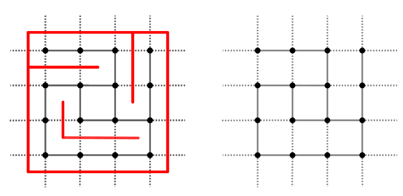
Figure 1: An example of a maze is represented as a numerical grid. Maze walls are represented by a red line, and a possible location in the maze where an agent can stand is represented by black nodes. The edges between those nodes are used only to provide information about whether the two nodes are adjacent or not, a full black line represents that there is a real connection between two nodes, and a dotted black line represents that there is an obstacle between two nodes.

3.2 Agent motion control

Since we focus on the exploration of the maze and the cooperation of the agents, in this paper we use the simplest first-order kinematic model for the agents’ motions, which neglects the agents’ mass and inertia and it is constrained to orthogonal motion. We also introduce a new method for collision avoidance when moving through the maze. This algorithm allows agents to stop and wait until another agent is no longer blocking their motion. We have also left the option to allow collisions when an application of the algorithm requires it.

In the beginning, the maze is unknown and the main priority of the agent system is to explore the maze. Agents explore the surroundings of their initial positions with limited knowledge, focusing solely on neighboring nodes that are within their awareness. The agents start their movement from initial positions and the primary goal is to search the unknown maze and find the exit. They can only move one step up, down, left, or right if there is no wall preventing them from doing so. This means that the directions in (1) are limited to only 4 possibilities, and the agent chooses the one with the greatest potential (which corresponds to the gradient $\nabla\mathbf{u}$ from (1)). Agents cannot go or see through walls, but they can exchange information about their position and the explored parts of the maze.

Time domain is discrete $t_{i}=i,i=0,\ldots,n$. After each time step the numerical domain and the set of indexes $I(t_{k})$ is updated with new nodes. Therefore, the trajectories of the agents can be described by functions $z_{p}:\mathbb{N}_{0}\to\mathbb{N}$, for $p=1,2,\ldots,N$.

Since the spatial and temporal domains are discretized, we can represent the coverage function $c(x_{i,j},t_{k})$ at time step $t_{k}$ for the maze node $x_{i,j}$ as a cumulative sum of ones and zeros, depending on the number of times the agents have visited the node $x_{i,j}$ by time step $t_{k}$. For each agent that visits the maze node $x_{i,j}$ at each time step, 1 is added, and 0 in all other cases.

The source term $s$ in this, discrete, case is represented as a non-negative scalar field

$$s(x_{i,j},t_{k})=max(0,1-c(x_{i,j},t_{k}))\cdot S(t_{k})$$

which emphasizes the insufficiently covered maze nodes $x_{i,j}$ at time step $t_{k}$, where $S(t_{k})$ is a scale factor that can be chosen to help the convergence of a linear solver. In are numerical examples we used $S(t_{k})=|I(t_{k})|$.

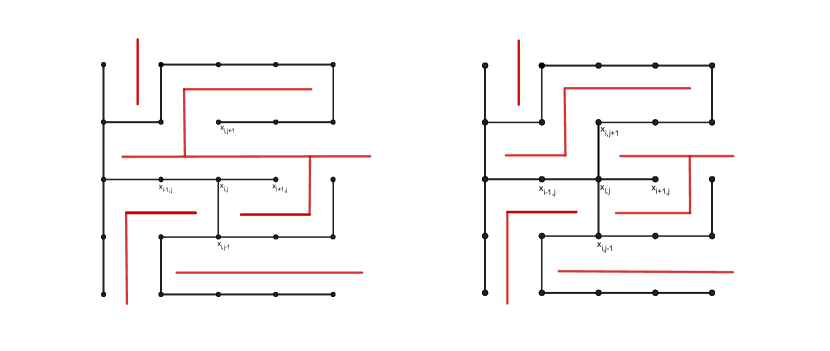
Figure 2: Examples of neighbors of $x_{i,j}$ node depending on the arrangement of the maze walls. Maze walls are presented with red lines, and maze nodes and connections between them are presented with black nodes and lines respectively.

Figure 2, on the right, shows an example of maze node $x_{i,j}$ which has no obstacle towards any of neighboring nodes, so value $u_{i,j}$ of the solution of PDE equation (2) can be obtained by discrete finite difference approximation as

$$\frac{u_{i-\delta x,j}-2u_{i,j}+u_{i+\delta x,j}}{(\delta x)^{2}}+\frac{u_{i,j-\delta y}-2u_{i,j}+u_{i,j+\delta y}}{(\delta y)^{2}}=\alpha\cdot u_{i,j}-s(x_{i,j},t_{k})$$

because we use $\delta x=\delta y=1$ we get

$$(4+\alpha)u_{i,j}-u_{i-1,j}-u_{i+1,j}-u_{i,j-1}-u_{i,j+1}=s(x_{i,j},t_{k}).$$ (4)

It remains to explain what to do with the more complicated case where there is an obstacle between a node and at least one of its neighboring nodes, such as in Figure 2 on the left. Given the structure of the maze shown in Figure 1, we can consider those disconnections/walls between the nodes as boundaries and impose Neumann boundary conditions there because, from the point of view of the conductive model, Neumann boundary condition actually represents an ideal insulating wall, a barrier in the domain through which heat is not conducted.

In the particular case in Figure 2 at the left side, we can set up the Neumann boundary condition on the top of the node at position $(i,j)$. Second-order approximation of the Neumann boundary condition

$$\frac{\tilde{u}_{i,j+\delta y}-u_{i,j-\delta y}}{2\delta y}=0$$

where $\tilde{u}$ marks a temporary node, modifies the (4) to obtain:

$$(4+\alpha)u_{i,j}-u_{i-1,j}-u_{i+1,j}-2u_{i,j-1}=s(x_{i,j},t_{k}).$$ (5)

There is one more interesting case in Figure 2 on the left and it concerns the node at position $(i,j+1)$, we set up Neumann boundary condition on the top, bottom, and at the left side of the node. Due to the Neumann boundary condition partial derivative in the vertical direction vanishes, and the equation reduces to a 1D case:

$$(2+\alpha)u_{i,j+1}-2u_{i+1,j+1}=s(x_{i,j},t_{k}).$$ (6)

All special cases (4),(5),(6) can be written in a general form which holds for all nodes:

$$(\sum_{l\in L}a_{i,j}(l)+\alpha)u_{i,j}-\sum_{l\in L}a_{i,j}(l)u_{l}=s(x_{i,j},t_{k}),$$ (7)

where $L=\{(i+1,j),(i-1,j),(i,j+1),(i,j-1)\}$. Interface function $a_{i,j}(l)\in\{0,1,2\}$ depends on the structure of walls around the node $(i,j)$ and it holds $0\leq\sum_{l\in L}a_{i,j}(l)\leq 4$. The equation in (7) holds for nodes with all four neighboring nodes and in the absence of some neighboring nodes by applying Neumann boundary conditions to the finite difference approximation of the derivatives in (2). The solution of this system of linear equations is a scalar field $u$ which is used to control the agents in the maze.

Each agent moves one step at time $t_{k}$ to a neighboring node where a scalar field $u$ has a larger value. A simple iterative numerical method can be used to approximate the solution by successive averaging over each node:

$$u^{r+1}_{i,j}=\frac{\sum_{l\in L}a_{i,j}(l)u^{r}_{l}+s(x_{i,j},t_{k})}{\sum_{l\in L}a_{i,j}(l)+\alpha},$$ (8)

where $r$ counts iterations until convergence.

Equation (8) describes a Jacobi iterative method. The iterations are very simple and can be performed in parallel using the cumulative computational power of the multi-agent system. Simple iterations allow us to solve a growing domain without re-meshing, as new numeric nodes are simply added to a list and assigned to one of the processors with the lowest load.

Theorem 3.1.

Iterations defined in (8) converge to a unique solution $\tilde{u}$ for arbitrary initial values of $u$. Furthermore, the visited node can’t be a local maximum of $\tilde{u}$.

Proof.

Equation (8) is a Jacobi iterative solver for a linear system $Au=s$ which comes from a finite difference approximation of equation (2). The matrix of the linear system $A$ is strictly diagonally dominant for $\alpha>0$ from which it follows that the solution is unique and the Jacobi iteration converges for arbitrary initial vector $u$.

Let’s suppose that $u$ attains a local maximum value at some node $u_{i,j}$ which was visited before time $t_{k}$ it follows that $s(x_{i,j},t_{k})=0$. From (8) it follows

$$u_{i,j}=\frac{\sum_{l\in L}a_{i,j}(l)u_{l}}{\sum_{l\in L}a_{i,j}(l)+\alpha}<\frac{\sum_{l\in L}a_{i,j}(l)u_{l}}{\sum_{l\in L}a_{i,j}(l)}\leq\max_{l\in L}(u_{l})$$

which is a contradiction. It follows that the maximum is attained at some unvisited node if it exists. ∎

From the theorem, it appears that simple iterations can be used to calculate the potential field that can be used to navigate the agents throughout the maze. As agents move toward the local maximum, they will continue to do so until they have visited all available nodes. In addition, the iterations are very simple, and we do not need to actually construct and expand the linear system at each time step, which makes domain growth easy to implement with a very low memory load.

There is a downside to this approach, the convergence of the Jacobi method slows down for a large numerical domain. This convergence can be improved using Gauss-Seidel iterations which make use of freshly calculated values of the state vector for each component of the state vector $u$. Although Gauss-Sidel should improve convergence, parallelization of the iterations is not as simple as the Jacobi method. In our implementation, we used successive over-relaxation (SOR) Gauss-Seidel iterations which improves the convergence of the Gauss-Sidel method but depends on the over-relaxation parameter $\omega$. The parallelization of iterations is accomplished by splitting the discovered nodes into two sets using a black-and-red strategy. We form two sets of nodes $B=\{(i,j)\in I(t_{k})|i+j\textrm{(mod 2)}=0\}$ and $R=\{(i,j)\in I(t_{k})|i+j\textrm{(mod 2)}=1\}$. We can calculate the SOR Gauss-Sidel method in two successive steps:

$$u^{r+1}_{i,j}=u^{r}_{i,j}+\omega\left(\frac{\sum_{l\in L}a_{i,j}(l)u^{r}_{l}+s(x_{i,j},t_{k})}{\sum_{l\in L}a_{i,j}(l)+\alpha}-u^{r}_{i,j}\right),\textrm{for all }(i,j)\in B$$ (9)

$$u^{r+1}_{i,j}=u^{r}_{i,j}+\omega\left(\frac{\sum_{l\in L}a_{i,j}(l)u^{r+1}_{l}+s(x_{i,j},t_{k})}{\sum_{l\in L}a_{i,j}(l)+\alpha}-u^{r}_{i,j}\right),\textrm{for all }(i,j)\in R$$ (10)

Iterations in steps (9) and (10) are very simple and each of them can be calculated in parallel. The optimal choice of parameter $1<\omega<2$ improves the convergence by two orders of magnitude when compared to the Jacobi method.

In [20] and [21] one can find the optimal relaxation parameter for the Poisson equation with Dirichlet boundary conditions on a regular grid in two or more spatial dimensions. The optimal value of relaxation parameters which maximizes the convergence of the SOR method depends on the problem under consideration and the size of the domain but it is typically $1.5<\omega<2.$.

To the best of our knowledge optimal relaxation parameters for (9) and (10) on a rectangular grid for equation (2) with Neumann boundary conditions is an open problem. We determined the over-relaxation parameter experimentally and found that its optimal value for the presented problem is $1<\omega<1.5$ and it depends on heat conduction parameter $\alpha$.

Now that we know how $u$ is determined, we can write down the rules and algorithm for controlling the movement of the agents:

• Initially, the maze is unknown, agents appear at their initial positions, a random node is set as the exit of the maze, and the basic task of the agent system is to explore the maze and find the exit node.

• Agents have a defined order in which they make a choice of their next move, an agent that has an associated trajectory $\mathbf{z}_{1}$ at a given time $t$ decides first to which node it moves, while an agent associated with a trajectory $\mathbf{z}_{N}$ decides last to which node it moves to.

• The agent can move up, down, left, or right one step at a time.

• At the time $t$ the agent moves to the adjacent node with the largest value of the $u$.

• Additionally, the agent has the information if one of the other agents is currently standing on one of the neighboring nodes and does not consider this node for its next position if the anti-collision condition, hereafter referred to as AC, is on. If the agent has no better option, it can wait on the spot until its path is clear.

• When the agent’s new position is determined, that node is immediately marked as a visited node, so agents who have yet to step during time $t$ can update their data about newly visited nodes before starting to determine their new positions.

• At the end of time $t$ agents update their newly discovered nodes so that at the beginning of the $t+1$ time, complete data about visited and newly discovered nodes can be exchanged between all agents.

• The search ends when one of the agents have found the exit node or the maze is fully explored i.e. $\sum_{I(t)}S_{i,j}=0$.

initialization ;

for $t=0,\,t=\max_{t},\,t=t+1$ do

       exchange of information about discovered nodes between agents;

       upadate of a linear system;

       iteratively solve a linear system (9),(10) ;

       for $i=1,\,i=N,\,i=i+1$ do

             next$\_$pos for agent $i$ = non ocuppied neighbouring nodes where is the largest value of the scalar field $u$ or current position if all neigbouring nodes are ocuppied;

             agents $i$ new position is marked as visited node;

       end for

      if  exit node found  then

            break;

      else

            

       end if

      

end for

Algorithm 1 Maze exploration with collision avoidance mechanism

4 Results

The benchmark tests of the proposed algorithm are related to two different scenarios: Mapping an unknown maze - where the main goal is to visit all nodes in the maze, and searching an unknown maze to find a way out, i.e. an exit node. In the presented algorithm, a linear system is solved and the potential field is updated before each agent chooses the next step. For this reason, it is useful to check the influence of the AC condition. Therefore, for both scenarios, we first tested whether the results of the algorithm significantly depend on whether AC is on or off. For each scenario, we conducted tests where 5 agents appeared at random starting positions and then explored the unknown maze with the target task depending on the scenario (mapping the entire maze or finding the exit). We randomly created 100 tree-like mazes of dimension 10x10 (with a proportion of 45$\%$ obstacles) and 100 more passable mazes of dimension 10x10 and with a proportion of 30$\%$ obstacles, these mazes were created by tearing down the walls in the previously created tree-like mazes. The same setup is used to test the algorithm with AC. In the tests performed, it was found that the collision avoidance condition does not significantly affect the total time steps required to execute these scenarios.

Table 1 shows the arithmetic means of 100 tests for two different goals, on two maze types with AC on and off. The T-test for 2 dependent means with a significance level of $p=0.05$ shows that there is no significant difference between these means, so we can conclude that AC does not play a significant role in the number of steps required to find the exit or map the entire unknown maze.

These tests show that the search results of this algorithm do not need the AC to ensure efficient workload distribution. If the potential field were updated only once and the agents chose their next step independently, the AC would be necessary to prevent the agents’ paths from merging and them traveling together from then on.

	Finding exit		Maze mapping
Anti-collision condition (AC)	ON	OFF	ON	OFF
45$\%$ obstacle share	17.36	18.67	51.38	52.68
30 $\%$ obstacle share	13.67	13.31	36.51	37.29

Table 1: Average steps needed for mapping different maze types with different goals with AC turned ON and OFF.

4.1 Finding an exit

Our algorithm achieved good results mainly thanks to the good distribution of work between agents, as shown in Figure 3.

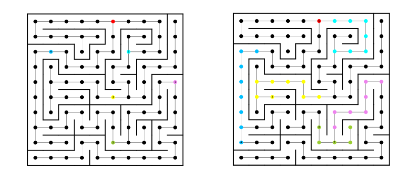
Figure 3: Example of division of work between 5 agents in finding a way out of a 10x10 maze with AC turned on. The nodes are colored according to the agent who visited them first. The exit is colored red. Unvisited/unmapped nodes are colored black. The initial positions of the agents are shown on the left side, and the distribution of work between the agents in the last step is shown on the right side.

We compare our algorithm with two alternative algorithms, the algorithm of Kivelevitch and Cohen [4], which works only for tree-like mazes (exactly one path from one maze node to another), and with the improved algorithm of Alian [5], which works for general mazes. We also compare the performance of our algorithm on unknown and known mazes.

4.1.1 Comparison with Kivelevitch and Cohen algorithm

The algorithm of Kivelevitch and Cohen is used to solve a problem in which a group of agents searches for a maze exit all starting from a single node and, once found, leads the entire group out of the maze through that exit. In searching for the exit, each agent follows a generalization of Tarry’s algorithm, except that all agents know which node has already been visited. Each agent follows the following rules:

• The agent should move to nodes that have not yet been traveled by another agent.

• If there are several such nodes, the agent should choose one at random.

• If there is no unvisited node (at least one agent has visited all candidate nodes), the agent should prefer a node that has not yet been visited by it.

• If the agent has already moved in all possible directions, or if it has reached a dead end, it should backtrack to a node that satisfies one of the previous conditions

• All steps should be logged by the agent as it moves along.

• When retreating, the nodes from which the agent has retreated should be marked as ”dead end”.

In their paper, Kivelevitch and Cohen use the same starting position for all agents, because once the first agent has found the exit, the part of the algorithm that is supposed to get all other agents to the exit begins. It is based on finding a common node on the path between the agent that found the exit and the other agent that is supposed to go to the exit, and if the agents do not start from the same starting position, there is no guarantee that they will have a common node on their way through the maze. Since we do not use this part of the algorithm for comparison (we stop the algorithm when the exit is found), it is possible to place agents in different starting positions and they will find the exit just as successfully.

To compare our algorithm with the algorithm of Kivelevitch and Cohen implemented for tree-type mazes, we performed our tests with mazes of dimensions 10x10 and 20x20 generated with a program written in Matlab and described in [4]. The mazes generated with this program can be represented as a tree, i.e. there is exactly one path from one maze node to another.

We observe a situation where an autonomous multi-agent system consisting of 1, 2, 3, 4, 5, 10, 15, and 20 agents searches an unknown maze for an exit. The initial positions of the agents were randomly created and maintained, so we used the same initial configuration of agents in the same maze to test both algorithms. We use our algorithm with AC turned off regardless of the fact that it gives worse results in this configuration according to Table 1 since Kivelevitch and Cohen’s algorithm also works with AC turned off. One of the 10x10 mazes used in this scenario is shown in Figure (3). We compare the average time (in steps) it took to find an exit in 250 tests. Figure 4 shows that our algorithm has a measurable advantage when more than one agent is present in the domain.

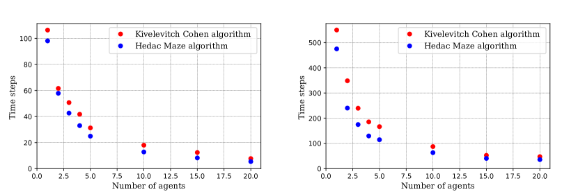
Figure 4: Our proposed algorithm (HEDAC) compared to the Kivelevitch-Cohen algorithm for finding maze exit. Average time steps for finding an exit with the same setup using both algorithms in a 10x10 maze (left) and a 20x20 maze (right).

We performed a T-test for two dependent means at a significance level of $p=0.05$ for the data obtained, and these tests showed that the difference between the results of our proposed algorithm and the Kivelevitch-Cohen algorithm shown in Figure 4 was significant for all cases except when we used two agents in a 10x10 maze, in which case the difference between these results proved not to be significant.

4.1.2 Comparison with Alian algorithm

The Alian algorithm can be considered an improvement of the Kivelevitch and Cohen algorithms. It works for all maze types and solves the problem of finding the exit of the maze and then getting the whole group out of the maze through that exit. In this algorithm, the nodes of the maze are colored in three colors: white are unvisited maze nodes, grey are visited maze nodes, and black are maze nodes from which there is only one way to the exit.

When searching for the exit, assuming that an agent detects a neighboring maze node with its sensor, each agent follows the following rules:

• For each currently visited maze node, there is occupied flag is set to true so that other agents know they cannot go there.

• If there is a neighboring maze node that has not yet been visited by any agent (white), the agent should go there.

• If there are several such nodes, the agent should choose one at random.

• If there is no node that has not been visited by any agent yet, the agent should prefer a node that has not been visited by it yet.

• If there are several such nodes, the agent should choose one at random.

• If the agent has already traveled in all possible directions, the agent will choose the node that has been visited the least by it.

• If there is only one neighboring maze node that can be visited, but it is currently occupied, the agent should wait at its current maze node until it becomes free

• If there is only one way to leave the current node, and all other directional are obstacles or black nodes, the agent marks the current node as a black node so that other agents cannot move there.

A detailed algorithm can be seen in [5]. We observe a situation where an autonomous multi-agent system consisting of 1, 2, 3, 4, 5, 10, 15, and 20 agents searches an unknown maze for an exit. The initial positions of the agents and the structure of the maze were randomly created and maintained, so we used the same initial configuration of agents in the same maze to test both algorithms. We use our algorithm with AC on, since the Alian algorithm does not impose a collision constraint. We compare the average time required to find the exit from the maze using both algorithms. All the results of our proposed algorithm and the Alian algorithm, shown in Figure 5, were found to be significantly different by the T-test performed for 2 dependent means with significance level $p=0.05$, except for the test with 20 agents in a 10x10 maze.

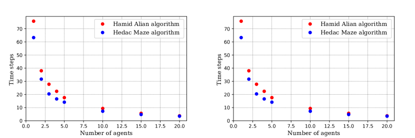
Figure 5: Our proposed algorithm (HEDAC) compared to the Alian algorithm for finding maze exit. Average time steps for finding an exit with the same setup with both algorithms in a 10x10 (left) and 20x20 (right) maze.

4.1.3 Finding a way out from known and unknown maze

With minor changes to the input data, the algorithm also works well to find the exit in a maze where the wall structure is exposed but the exit is hidden at a random node with uniform distribution. Similar to the previous comparisons, we performed 250 tests for each situation in which an autonomous multi-agent system consisting of 1, 2, 3, 4, 5, 10, 15, and 20 agents searches in an unknown and known maze. The initial positions of the agents and the structure of the maze were randomly created and stored so that we could use the same initial configuration of the agents in the same maze to test both algorithms.

We compare the average time in the Figure 6, where we can see that there is almost no difference between the two cases. Also, we performed a T-test for two dependent means at a significance level of $p=0.05$ for the obtained data, and it proves that there is no significant difference between them. We should point out here that in the case of non-uniform distribution of exit nodes, the case of the known maze would have a clear advantage.

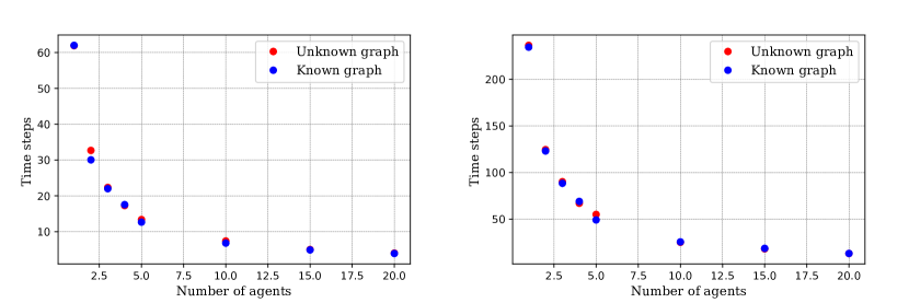
Figure 6: Comparison of the efficiency of our proposed (HEDAC) algorithm on known and unknown mazes of dimensions 10x10 (left) and 20x20 (right). Average time steps for finding an exit from the same maze, depending on whether it is previously known or unknown.

4.1.4 Scalability of our proposed algorithm for finding exit

We will discuss scalability in terms of dividing the work between multiple agents, more specifically we will discuss scalability in terms of the percentage of average steps required to find an exit with a multi-agent system compared to the average steps required to find an exit with a single agent. The division of work between agents shown in Figure 3 indicates that our proposed algorithm scales well for exploring mazes and finding the exit in an unknown maze. We can use data from previous tests to discuss the scalability of our proposed algorithm in detail. The results of our algorithm compared to the algorithms of Kivelevitch and Cohen, shown in Figure 4, are processed in Table 2. From Table 2, it can be seen that the average number of total time steps required to find the exit from the tree-type maze with the anti-collision condition turned off decreases significantly with the use of more agents. For both maze sizes, it can be seen that when two agents are used, the total number of agent steps needed to find the exit requires less than $20\%$ more steps compared to the case with one agent. When using 3 and 4 agents, the total time decreased significantly and the total number of steps needed to find the exit remained about the same as in the 2 agent case. With a larger number of agents, the total time continues to decrease in both cases, but the total number of agent steps shows that efficiency actually increases in the $10\times 10$ maze, while it decreases as expected in the larger maze. The tree-type maze shows a skewed picture of scalability analysis, but it shows that the algorithm works well with more agents and the division of work between agents is good.

The performance is even better when we use a multi-agent system with AC on a general maze with fewer obstacles. We use the results of our algorithm compared to Alian’s algorithm, which are shown in Figure 5. As can be seen in Table 3 where the results are processed, with 2 agents the total time is almost halved in addition to the situation where we use one agent, with 3 and 4 agents the scaling continues so that it takes about 1/3 and 1/4 of the time to find the exit with one agent respectively. We should note that the scaling is almost ideal for both maze sizes even with a larger number of agents, which is very interesting.

It is important to mention that we performed scalability tests with previously obtained data for specific types of mazes and with AC condition turned on and off, depending on the conditions in the algorithms we compared with and according to the Table 1, it appears that the AC condition turned off would give even better absolute results in Table 3, just as the AC condition turned on would give even better absolute results in Table 2

Maze size	10x10		20x20
Number of	Total time	Total agent	Total time	Total agent
agents	steps	steps	steps	steps
1	98.076	98.076	475.052	475.052
2	57.856	115.712	240.196	480.392
3	42.632	127.896	174.872	524.616
4	33	132	129.572	518.288
5	24.92	124.6	114.664	573.32
10	12.784	127.84	63.344	633.44
15	8.216	123.24	40.508	607.62
20	5.424	108.48	35.784	715.68

Table 2: Scalability of our algorithm with AC turned off in a tree-type maze, e.g., 45$\%$ obstacles share. Average total number of time steps and average total number of agent steps for finding an exit with a multi-agent system.

Maze size	10x10		20x20
Number of	Total time	Total agent	Total time	Total agent
agents	steps	steps	steps	steps
1	63.264	63.264	243.344	243.344
2	31.664	63.328	126.876	253.752
3	20.412	61.236	85.228	255.684
4	16.588	66.352	62.488	249.952
5	14.128	56.512	50.948	254.74
10	72.36	72.36	24.664	246.64
15	4.748	71.22	17.772	266.58
20	3.476	69.52	14.804	296.08

Table 3: Scalability of our algorithm with AC turned on , with 30$\%$ obstacles share. Average total number of time steps and average total number of agent steps for finding an exit with multi-agent system.

4.2 Mapping an unknown maze

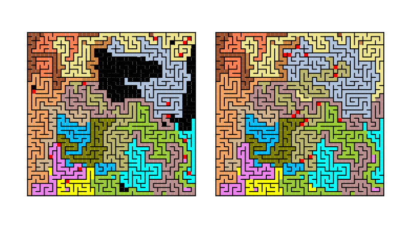
Figure 7: Example of division of work between 15 agents mapping an unknown 40x40 maze at time step 250 (left) and at the last time step 425. The anti-collision condition is turned off andthe nodes are coloured according to the agent who visited them first.

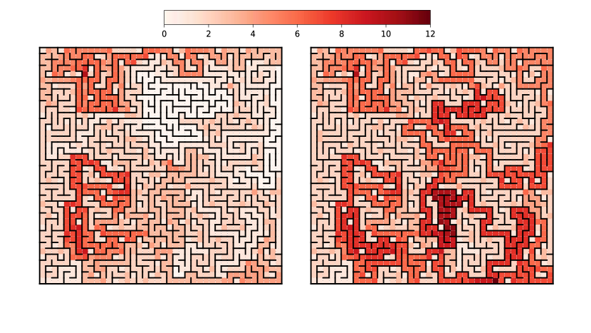
Figure 8: Coverage values indicating cumulative visits for each maze node at time step 250 (left) and at the final, time step 425 (right).

Here we observe a situation where a multi-agent system is used to map an unknown maze. Agents appear at randomly selected positions/maze nodes and explore the maze until all maze nodes are visited. AC is off.

To create the maze, we used a depth-first search-based maze generator algorithm described in [22]. In Figure 7, we can see how at the beginning the agents map only the initial positions and see only the nodes/walls that are right next to their initial nodes. Step by step they visit other nodes and exchange information about the visited and discovered nodes so that in the last step the structure of the whole maze is gradually revealed. In Figure 7, the division of work between 15 agents can be seen at step 250, which is about halfway to the final step, and at the final step 425, when the entire maze is mapped. The agents do not know how the maze is constructed in the black areas in Figure 7, while the maze nodes that were first visited and mapped by certain agents are colored in the color assigned to those agents.

We also tracked the cumulative function of traversing each node; for each agent that steps on the node, the corresponding function value was increased by 1, making it easy to track which nodes were visited the most at each time step. Figure 8 shows the progression of the cumulative function step by step, from the least visited nodes (the lightest shades of red) to the most visited nodes (darker shades of red).

To test this part of the application of the algorithm, we observed the average time required to discover all nodes in three mazes with different properties.

We performed the tests with two mazes of size $10\times 10$, one of which is a maze that has only one path from one node to another (we call it a tree-type maze, it has an obstacle fraction of 45$\%$), and another, more passable maze with an obstacle fraction of $30\%$. We obtained this maze by tearing down some of the walls in the first maze we created. The initial positions of the agents are random, and we used the same initial configuration of agents to explore both mazes. Each test was run 500 times with the same scenario, the same number of agents, and the same maze with AC off.

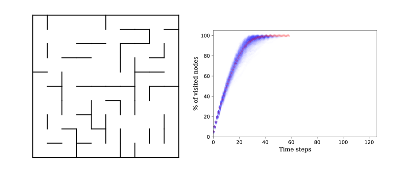
Figure 9: Percent of visited nodes of a 10x10 tree-type maze with 45$\%$ obstacles share explored by 5 agents, anti-collision condition is off.

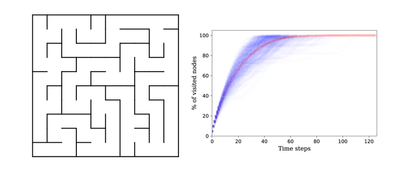
Figure 10: Percent of visited nodes of 10x10 maze with 30$\%$ obstacles share, explored by 5 agents, anti collision condition is off.

In 9 and 10, it can be seen that in the first steps for both mazes, the average percent of visited nodes increases almost linearly, while the result is even better with fewer obstacles, as expected. Thus, although this is not the primary task of our proposed algorithm, it has been shown to be capable of mapping the entire maze.

5 Conclusion

The algorithm presented proved to be robust, adaptable, scalable, and computationally inexpensive. The algorithm does not need to be adapted for each test, except for the parameter alpha, which emphasizes global or local search of the multiagent system. The AC procedure can be improved, but this will certainly not have a large impact on the overall average result. In future work, we will generalize the algorithm to graph search and monitoring, which is an obvious generalization that allows many different applications. In addition, optimal parameters for the SOR-Gauss-Sidel method could be calculated for this particular application.

Appendix

The entire process of mapping the maze, as well as the increase in the value of the cumulative function associated with the problem shown in Figure 7, can be viewed in the following videos:

• HEDAC maze exploration: Example of work division between 15 agent mapping unknown 40x40 maze

• HEDAC maze exploration: Cumulative function of crossing over each maze cell

References

- [1] B.Rahnama, A.Elci, C.Ozermen, Design and implementation of cooperative labyrinth discovery algorithms in multi-agent environment, in: 2013 The International Conference on Technological Advances in Electrical, Electronics and Computer Engineering (TAEECE), 2013, pp. 573–578. doi:10.1109/TAEECE.2013.6557338.
- [2] C. E. Shannon, Presentation of a maze-solving machine, in: Cybernetics, Transaction of the Eight Conference, Josiah Macy, Jr. Foundation, 1951, pp. 173–180.
- [3] A. M. Sadik, M. A. Dhali, H. M. Farid, T. U. Rashid, A. Syeed, A comprehensive and comparative study of maze-solving techniques by implementing graph theory, in: 2010 International Conference on Artificial Intelligence and Computational Intelligence, Vol. 1, IEEE, 2010, pp. 52–56.
- [4] E. H. Kivelevitch, K. Cohen, Multi-agent maze exploration, Journal of Aerospace Computing, information, and communication 7 (12) (2010) 391–405.
- [5] H. Alian, Multi-agent asynchronous real-time maze-solving, Ph.D. thesis, University of Alberta (2022).
- [6] O. Khatib, Real-time obstacle avoidance for manipulators and mobile robots, The international journal of robotics research 5 (1) (1986) 90–98.
- [7] B. H. Krogh, A generalized potential field approach to obstacle avoidance control, in: SME COnference Proceedings Robotics Resarch: ”The Next Five Years and Beyond”, Bethlehem, Pennsylvania, SME, 1984.
- [8] C. F. Thorpe, Path relaxation: Path planning for a mobile robot, in: Proceedings of the AAAI Conference on Artificial Intelligence, Vol. 4, AAAI, 1984, p. 318.
- [9] B. H. Krogh, C. E. Thorpe, Integrated path planning and dynamic steering control for autonomous vehicles, in: Proceedings of the 1986 IEEE International Conference on Robotics and Automation, San Francisco, California, IEEE, 1986, pp. 1664– 1669.
- [10] P. Vadakkepat, K. C. Tan, W. Ming-Liang, Evolutionary artificial potential fields and their application in real time robot path planning, in: Proceedings of the 2000 congress on evolutionary computation. CEC00 (Cat. No. 00TH8512), Vol. 1, IEEE, 2000, pp. 256–263.
- [11] D. Yagnik, J. Ren, R. Liscano, Motion planning for multi-link robots using artificial potential fields and modified simulated annealing, in: Proceedings of 2010 IEEE/ASME International Conference on Mechatronic and Embedded Systems and Applications, IEEE, 2010, pp. 421–427.
- [12] S. Ivić, B. Crnković, I. Mezić, Ergodicity-based cooperative multiagent area coverage via a potential field, IEEE transactions on cybernetics 47 (8) (2016) 1983–1993.
- [13] S. Ivić, A. Andrejčuk, S. Družeta, Autonomous control for multi-agent non-uniform spraying, Applied Soft Computing 80 (2019) 742–760.
- [14] T. Löw, J. Maceiras, S. Calinon, drozbot: Using ergodic control to draw portraits, IEEE Robotics and Automation Letters 7 (4) (2022) 11728–11734.
- [15] S. Ivić, Motion control for autonomous heterogeneous multiagent area search in uncertain conditions, IEEE Transactions on Cybernetics 52 (5) (2020) 3123–3135.
- [16] S. Ivić, A. Sikirica, B. Crnković, Constrained multi-agent ergodic area surveying control based on finite element approximation of the potential field, Engineering Applications of Artificial Intelligence 116 (2022) 105441.
- [17] S. Ivić, B. Crnković, L. Grbčić, L. Matleković, Multi-uav trajectory planning for 3d visual inspection of complex structures, Automation in Construction 147 (2023) 104709.
- [18] Y. Zheng, C. Zhai, Distributed coverage control of multi-agent systems in uncertain environments using heat transfer equations, arXiv preprint arXiv:2204.09289 (2022).
- [19] C. Bilaloglu, T. Löw, S. Calinon, Whole-body exploration with a manipulator using heat equation, arXiv preprint arXiv:2306.16898 (2023).
- [20] Fundamentals of Matrix Computations, 2nd Edition, John Wiley & Sons, Ltd, 2002. doi:https://doi.org/10.1002/0471249718.ch7.
- [21] S. Yang, M. K. Gobbert, The optimal relaxation parameter for the sor method applied to the poisson equation in any space dimensions, Applied mathematics letters 22 (3) (2009) 325–331.
- [22] https://scipython.com/blog/making-a-maze/.