View-Independent Adjoint Light Tracing for Lighting Design Optimization

Abstract.

Abstract

Controlling light is a central element when composing a scene, enabling artistic expression, as well as the design of comfortable living spaces. In contrast to previous camera-based inverse rendering approaches, we introduce a novel method for interactive, view-independent differentiable global illumination. Our method first performs a forward light-tracing pass, starting from the light sources and storing the resulting radiance field on the scene geometry, representing specular highlights via hemi-spherical harmonics. We then evaluate an objective function on the entire radiance data and propagate derivatives back to the lighting parameters by formulating a novel, analytical adjoint light-tracing step. Our method builds on GPU ray tracing, which allows us to optimize all lighting parameters at interactive rates, even for complex geometry. Instead of specifying optimization targets as view-specific images, our method allows us to optimize the lighting of an entire scene to match either baked illumination (e.g., lightmaps), regulatory lighting requirements for work spaces, or artistic sketches drawn directly on the geometry. This approach provides a more direct and intuitive user experience for designers. We visualize our adjoint gradients and compare them to image-based state-of-the-art differentiable rendering methods. We also compare the convergence behaviour of various optimization algorithms when using our gradient data vs. image-based differentiable rendering methods. Qualitative comparisons with real-world scenes underline the practical applicability of our method.

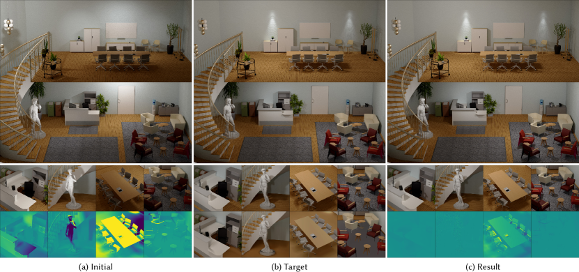
Figure 1. Optimizing lighting design parameters for a large office scene with our view-independent differentiable light-tracing method: Starting from an initial lighting setup (a) and a given ground-truth illumination target on the scene geometry (b), we perform gradient-based optimization, which closely recovers the ground truth in our solution (c). The small images show close-up views of the scene (middle row) and the difference to the target (last row). The last row (b) also shows the target illumination itself as represented in our radiance data structure used for optimization.

1. Introduction

Lighting plays an often overlooked but central role in our daily lives. It contributes to making a home feel relaxing, a workplace efficient, and is subject to important requirements in professional environments such as office spaces, hospitals, and factories. While artistic applications usually require manual luminaire placement, simple grid-like patterns are widespread in office spaces. Both scenarios can benefit from automated design, reducing the workload on artists, or producing more comfortable office lighting respectively. Commercial lighting design tools, such as DIALux [2022] and Relux [2022], are widely used, but limited to simple light interactions and still require manual editing of luminaires to achieve the desired result.

Forward rendering, i.e., simulating light transport in a 3D scene according to the rendering equation, has a long-standing history in computer graphics. Conversely inverse rendering methods aim to match a scene’s appearance to one or more target images. While these view-dependent (differentiable) rendering approaches could, in principle, address lighting design problems, they quickly become problematic for complex scenes, as many cameras would be required to capture all areas of interest. Additionally, this approach would raise the question of how many (and where) cameras should be (optimally) placed, and how to define illumination targets for them.

Currently, no solution for view-independent (i.e., camera-free) differentiable rendering exists. Extending camera-based renderers (Mitsuba, PSDR) to view-independent optimization is not trivial: we require a spatio-temporal data structure that can be updated quickly, the most efficient tracing approach (path tracing vs. light tracing) needs to be analyzed, and we need an analytical (adjoint) gradient formulation, than can be efficiently evaluated on the GPU, to make interactive optimization feasible.

In this paper, we propose an interactive and fully view-independent inverse rendering framework. The absence of a predefined camera view motivates a light-tracing global-illumination method, instead of more common path-tracing approaches. Our light tracing approach yields improved runtime performance and optimization convergence in our tests. While a differentiable path-space formulation is, in principle, also applicable to paths constructed via light tracing [Zhang et al., 2020], differentiating light tracing itself has not been addressed in previous work. Furthermore, our tests show that applying AD (or an equivalent analytical differentiation) to light tracing suffers from systematic errors that prevent optimization convergence. Conversely, our view-independent adjoint light-tracing method convergences reliably, and enables an efficient GPU-accelerated implementation.

Building upon our adjoint gradient formulation, we also introduce a visualization of how each point on the scene geometry contributes to the overall derivative of the optimization objective for a user-selected parameter. We compare this adjoint visualization to a standard (non-adjoint) visualization of derivatives.

In summary, we present the following contributions in this paper:

• An efficient adjoint gradient formulation for differentiable light tracing, and

• an efficiently updatable view-independent radiance data structure.

• This combination allows us to solve lighting design optimization tasks, while taking global illumination into account.

• We also present a novel visualization of point-wise adjoint gradient contributions, which helps us to evaluate our method.

2. Related Work

Here we briefly summarize the most relevant works on global-illumination rendering, before discussing recent advances in differentiable rendering. Furthermore, we introduce approaches that have investigated the lighting design problem from other directions, such as procedural modelling.

2.1. Forward rendering

In the following, we classify related work in four categories, as illustrated in the inset image. Path tracing, one of the most fundamental methods for physically-based rendering, applies Monte Carlo integration to solve the rendering equation [Kajiya, 1986; Veach, 1998]. Similar methods have been extensively used to render physically realistic images (category a). Pre-computed light-transport methods, on the other hand, such as radiosity [Goral et al., 1984; Greenberg et al., 1986], focus on solving global illumination for all surfaces in a 3D scene (category b) rather than for a view-dependent image.

More recently, these radiosity methods have been extended to incorporate glossy surfaces [Sillion et al., 1991; Sloan et al., 2002; Krivanek et al., 2005; Hašan et al., 2009; Omidvar et al., 2015] and also enable fast incremental updates allowing for interactive frame rates [Luksch et al., 2019]. We take inspiration from these approaches, constructing a spatio-directional radiance data structure in order to enable view-independent differentiable rendering (category d). The key ideas of our adjoint light tracing approach would in principle also be applicable to other pre-computed light-transport methods and radiance-field data structures, such as the recent work by Yu et al. [2021], as well as photon tracing, virtual point light, or light probe approaches.

2.2. Differentiable rendering

Previous work in (physically-based) inverse rendering has, so far, focused on camera-based methods (category c), where the goal is to optimize scene parameters (e.g., materials, textures, or geometry), such that the resulting image matches a given target [Gkioulekas et al., 2013; Khungurn et al., 2015; Gkioulekas et al., 2016; Liu et al., 2018; Li et al., 2018; Zhang et al., 2019; Nimier-David et al., 2019, 2020; Zeltner et al., 2021]. These methods define an optimization objective on the difference between a rendered and a target image. Previous work has strongly focused on optimizing textures, material parameters, or local shapes. While optimizing luminaire placement shares similarities with shape optimization, lighting parameters affect the illumination more globally throughout the scene.

Pioneering works in differentiable path tracing [Nimier-David et al., 2019; Loubet et al., 2019] have relied on code-level automatic differentiation (AD), recording a large computation graph, which is then traversed in reverse to compute the objective function gradient. However, AD fails for standard light tracing, because each light ray carries a fixed amount of radiative flux (power) independently of its direction, or distance traveled. Consequently, parameters that affect these quantities (but not the per-ray flux) cannot be correctly differentiated with AD. The PSDR approach [Zhang et al., 2020] side-steps this issue by moving the evaluation of radiative transport to a path-space formulation. Their implementation re-evaluates entire paths after construction and applies AD to compute derivatives of radiance contributions. One of our key insights is that we can take inspiration from their “material-form differential path integral” and construct a differentiation of light tracing itself (and similar methods) for lighting parameters. Furthermore, we also formulate an analytical adjoint state per ray, instead of using automatic differentiation, which allows for an efficient GPU-based implementation.

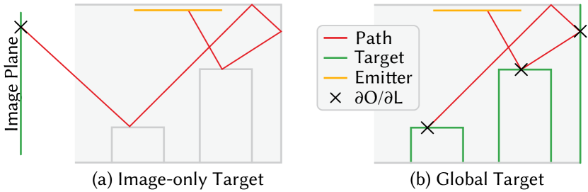
Figure 2. Image-based inverse rendering defines the optimization target on the image plane (a); our view-independent approach distributes this target throughout the scene (b). Our adjoint light tracing method collects partial derivatives at each light bounce (instead of considering only the image).

The basic idea of adjoint methods (also known as backpropagation in machine learning) is to reverse the flow of information through a simulation to find objective function gradients with respect to optimization parameters [Bradley, 2019; Geilinger et al., 2020; Stam, 2020]. For path tracing, Mitsuba 3 [Jakob et al., 2022] provides a similar adjoint method, called “radiative backpropagation” [Nimier-David et al., 2020], which avoids the prohibitive memory cost of AD. They extend this approach to the re-parameterized “path-replay backpropagation” integrator [Vicini et al., 2021]. In our lighting optimization tests, however, we observe reduced convergence rates for this method, compared to their AD version (using the latest available version of Mitsuba 3).

In our view-independent case, we find that (differentiable) light tracing often outperforms path tracing in terms of optimization convergence behaviour. As illustrated in Fig. 2, instead of transferring one radiance sample per path from a light source to a sensor, we update our radiance data at each ray-surface intersection and accordingly collect objective function derivatives from each of these locations in our adjoint tracing step, thereby using samples more efficiently. To our knowledge, we present the first view-independent, differentiable light tracing, inverse rendering method.

One problem that has received a lot of attention recently is how to differentiate pixel values in the presence of discontinuous integrands due to silhouette edges or hard shadows. Various strategies to resolve these issues have been proposed, such as reparametrizing the discontinuous integrands [Loubet et al., 2019], repositioning the samples around discontinuous edges [Bangaru et al., 2020; Zeltner et al., 2021], or separating the affected integrals into interior and boundary terms and applying separate Monte-Carlo estimators to each part [Zhang et al., 2020; Yan et al., 2022]. In this work we do not address the discontinuity problem explicitly. Our comparisons to image-based methods do not indicate improved convergence for lighting optimization when using existing discontinuity handling methods over standard differentiable rendering. This behaviour is likely due to the strong global coupling between lighting parameters, i.e., changing any parameter typically affects the solution in a large portion of the scene, reducing the effect of discontinuous edges on the total gradient. Nevertheless, handling discontinuous integrands in the context of view-independent light tracing is an interesting direction for future work.

For comparisons to related work, we have implemented a reference differentiable path tracer working on our view-independent data structure (without discontinuity handling). We also compare to existing image-based methods by restricting our objective function to consider only surfaces that are visible by the camera. In this way we separate the performance of the differentiation method from the benefits of operating on a larger global target. At this time, it appears that no existing method could address lighting design optimization in large scenes and at interactive rates.

2.3. Lighting design

In our work, we specifically consider the problem of designing lighting configurations, which has also been extensively explored in computer graphics and tackled from many different perspectives. Most approaches initially used variations of the sketching metaphor for user interaction, but were often limited to simple scenes with a small number of objects and viewpoints. These approaches include sketching the shape of shadows to indirectly move light sources [Poulin et al., 1997] or painting highlights and dark spots to control light parameters in the scene [Shesh and Chen, 2007; Pellacini et al., 2007]. Our view-independent differentiable rendering framework brings the sketching metaphor to 3D, providing a more intuitive way to paint desired illumination directly into the scene. In this way, we avoid any problems that might occur if the user accidentally assigns conflicting objectives in images from different views that actually correspond to the same 3D location.

The lighting design problem has also been approached from a procedural point of view, optimizing the lighting parameters after expressing the scene in terms of constraints on illumination and luminaire placement [Schwarz and Wonka, 2014], or in terms of standard lighting guidelines and pairwise relationships with scene objects [Jin and Lee, 2019]. As we focus on continuous optimization, these methods could be used to estimate a starting configuration before further optimizing the parameters of the generated light sources. In case of complex or dynamic scenes, or when high performance is required, hierarchical solutions [Lin et al., 2013; Gkaravelis, 2016] have instead been used to model lighting configurations. These top-down approaches allow a more exhaustive overview of the possible solutions, but come at the cost of limitations on the number and type of parameters that can be optimized. More recent approaches include the user in the optimization process [Sorger et al., 2016; Walch et al., 2019] directly, instead of automatically operating on a predefined target. These methods interactively display the current illumination and provide information about where and how this configuration could be improved. The user is then free to choose which measures to take in order to bring the scene closer to the desired state. In the future, our approach could be integrated into such a user-centred editing framework to improve the design interaction between the user and the optimization system.

3. Problem statement

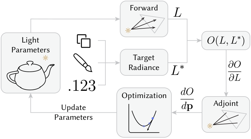
Figure 3. Illustration of our adjoint light-tracing optimization. See also Fig. 4 for further details on the forward and adjoint data flow.

We start with the well-known rendering equation [Kajiya, 1986], which models the exitant radiance $L({\mathbf{x}},{\omega_{o}})$ from a point $\mathbf{x}$ on a surface in the outward direction $\omega_{o}$ as

(1) $$L({\mathbf{x}},{\omega_{o}})={L_{e}}({\mathbf{x}},{\omega_{o}})+\int_{{\mathcal{H}^{2}}}{f({\mathbf{x}},{\omega_{i}},{\omega_{o}}){(\boldsymbol{\mathbf{n}}\cdot\omega_{i})}\;L_{i}({\mathbf{x}},{\omega_{i}})\;d{\omega_{i}}}.$$

The bidirectional reflectance distribution function (BRDF), ${f}$, encodes the material properties, and the incident radiance $L_{i}({\mathbf{x}},{\omega_{i}})$ at $\mathbf{x}$ is related to the radiance exitant from another point $\mathbf{x}^{\prime}$ by ${L_{i}}({\mathbf{x}},{\omega_{i}})=L({\mathbf{x}^{\prime}},{-\omega_{i}})$, such that $\mathbf{x}^{\prime}$ is the nearest ray-surface intersection when tracing a ray from $\mathbf{x}$ in direction $\omega_{i}$. Here, we focus on reflective light transport for brevity, but in principle, transmissive surfaces could be included in mostly the same way. Consequently, we restrict the directional integration to the hemisphere ${\mathcal{H}^{2}}$ instead of the entire (unit) sphere ${\mathcal{S}^{2}}$. We also do not consider any volumetric light-scattering effects.

We aim to support lighting design tasks by applying differentiable rendering and continuous optimization to minimize an objective function that measures the quality of a given lighting configuration. More formally, for this inverse design application, we consider objective functions $O$ of the form

(2) $$O(L)=\frac{1}{2}\int_{\Omega}{\frac{1}{{2\pi}}\int_{{\mathcal{H}^{2}}}{\alpha({\mathbf{x}},{\omega_{o}}){{\left({L({\mathbf{x}},{\omega_{o}})-{L^{*}}({\mathbf{x}},{\omega_{o}})}\right)}^{2}}\;d{\omega_{o}}}d{\mathbf{x}}},$$

where $L^{*}$ is our illumination target, $\alpha$ is a user-defined weighting function, and $L({\mathbf{x}},{\omega_{o}})$ must satisfy the rendering equation. We assume that the emitted radiance $L_{e}(\boldsymbol{\mathbf{p}})$—described by a given set of light sources—depends on various optimization parameters $\boldsymbol{\mathbf{p}}$. Therefore, the solution is also parameter-dependent, and our main task is to find local minima of the following optimization problem:

(3) $$\boldsymbol{\mathbf{p}}^{*}=\arg\min_{\mathbf{p}}O(L({\mathbf{p}})),{\text{~{}s.t.~{}}L\text{~{}satisfies Eq.~{}\eqref{eq:radiance}.}}$$

In order to address this problem, we compute an approximate solution, $L({\mathbf{x}},{\omega_{o}})$, on the surfaces of a virtual 3D scene in a forward rendering pass (§4.2). We then derive an adjoint (or backpropagation) rendering pass (§4.3) that allows us to compute derivatives of the optimization objective with respect to the parameters, $dO/d\boldsymbol{\mathbf{p}}$. Consequently, we are able to apply gradient-based continuous optimization methods to the lighting design problem.

4. View-independent adjoint light tracing

In the following sections, we first describe how we discretize the radiance data and optimization target (§4.1), how we update this data while light tracing (§4.2), and finally how we compute the objective gradient trough adjoint light tracing (§4.3).

4.1. Spatio-directional data structure

In order to represent the spatio-directional radiance field $L$ with a finite number of variables (or degrees of freedom, DOF), we first construct an appropriate interpolation scheme. We then use this scheme to find approximate solutions to Eq. ((1) ).

For the spatial component, we choose a piece-wise linear interpolation, as often used in finite element (and specifically radiosity) methods [Greenberg et al., 1986; Larson and Bengzon, 2013]:

(4) $$L({\mathbf{x}},{\omega_{o}})\approx\sum\nolimits_{k}{{L_{k}}({\omega_{o}}){\varphi_{k}}({\mathbf{x}})}.$$

Instead of single nodal values, however, we consider $L_{k}$ to be a directional function associated with the $k$-th mesh vertex (and consequently with the basis function $\varphi_{k}$).

For the directional component, we discretize each per-vertex function $L_{k}(\omega_{o})$ using a hemi-spherical harmonic (HSH) basis [Sillion et al., 1991; Gautron et al., 2004; Krivanek et al., 2005], specifically, the $2\pi$-normalized hemi-spherical harmonics ${H_{m}^{l}}$ [Wieczorek and Meschede, 2018]. Each directional function is consequently represented as

(5) $${L_{k}}({\omega_{o}})\approx\sum\nolimits_{l=0}^{l=n}{\sum\nolimits_{m=-l}^{m=l}{{L_{klm}}{H_{m}^{l}}({\omega_{o}})}},$$

where $n$ is the maximal order used in this approximation, which implies that for each vertex $k$, we require $(n+1)^{2}$ directional coefficients. Consequently, our spatio-directional approximation (using three colour channels, RGB) has $3m(n+1)^{2}$ degrees of freedom, where $m$ is the number of mesh vertices.

In contrast to previous work, we store exitant rather than incident radiance, because we define our optimization objective on the exitant radiance. This choice also allows for immediate preview visualization of the approximate radiance field. Note that our choice of spatial interpolation directly attaches data to the underlying mesh geometry, which can cause the triangulation to become visible in our preview visualization. In principle, a (bilinearly interpolated) texture-map approach, or higher order interpolations, as well as meshless bases [Lehtinen et al., 2008], would also be applicable here. Our primary goal is to solve inverse problems based on this discretization, whereas we produce high-quality output images via standard rendering methods. Therefore, we favour the simplicity of this discretization over alternatives and accept that it may cause some visual artifacts in preview images.

For completeness, we summarize the construction of ${H_{m}^{l}}$ in the supplementary material. Furthermore, for the special case $n=0$, we effectively ignore any directional dependence. In this case, which is sufficient for diffuse surfaces, our data structure contains simply vertex colours. Note that even if we choose $n=0$, our light tracing method may still include glossy materials when simulating indirect lighting. As with the spatial discretization earlier, there are of course other approaches that could be used for the directional discretization. In principle, our adjoint gradient calculations would apply similarly to other radiance field approximations, such as photon mapping, virtual point lights, or potentially neural radiance fields.

One key advantage of our discretization is that it can be efficiently modified: due to orthogonality of the basis functions, each radiance sample can be projected into our data structure independently. In the following section, we describe how we update the coefficients of our data structure for each radiance sample generated by light tracing.

Furthermore, discretizing the target radiance field in the same way yields target coefficients ${L_{klm}^{*}}$ and subsequently a discrete analog of the objective function, Eq. ((2) ):

(6) $$O(L)=\frac{1}{2}{\sum\nolimits_{klm}{{A_{k}}{\alpha_{k}}\alpha_{l}({L_{klm}}-L_{klm}^{*})^{2}}},$$

where$A_{k}$ is the area associated with vertex $k$, i.e, one third of the sum of adjacent triangle areas, and we have split the weights into a spatial and a directional component, $\alpha_{k}$ and $\alpha_{l}$ respectively. In this way, the weights $\alpha_{l}$ adjust the influence of each HSH band: over-weighting lower bands for example would emphasize low-frequency components of the reflected radiance. Similarly, $\alpha_{k}$ allows us to focus the attention of the optimizer on specific parts of the scene geometry. We use a painting interface to allow the user to specify $L_{klm}^{*}$ as well as $\alpha_{k}$.

In summary, our data structure stores exitant radiance via piece-wise linear spatial and HSH directional interpolation, providing the following important features: It allows us to efficiently update the data for each radiance sample (§4.2), and directly paint the target lighting in an interactive user interface. Furthermore, the derivative of Eq. ((6) ), ${\partial O/\partial L_{klm}}$ (used in §4.3) is straightforward to evaluate.

4.2. Forward light tracing

Having described our radiance field data structure in the previous section, we now focus on how we solve the rendering equation using light tracing and update the coefficients $\{L_{klm}\}$ of this data structure accordingly. We summarize this procedure in Alg. 1, and provide details of the derivation in the supplementary document.

For every light source, we sample $N$ exitant rays, each representing a radiant flux $\Phi_{r}$ leaving the light source, distributed according to the light’s emission profile, such that the sum of all these exitant samples equals the total radiative power of the light. Let ${{\mathbf{x}}_{0}}$ be the origin of a ray, which for point-shaped light sources is simply the light’s position. We then construct a light path up to a maximal number of indirect bounces, denoted as a sequence of ray-surface intersection points ${{\mathbf{x}}_{1}},\ldots,{{\mathbf{x}}_{i}},\ldots,{{\mathbf{x}}_{\text{max}}}$.

The incident flux $\Phi_{i}$ arriving at each hit point ${{\mathbf{x}}_{i}}$ is ${\Phi_{1}}={\Phi_{r}}$ (direct illumination) and

(7) $${\Phi_{i+1}}={\Phi_{i}}\;f_{i}(-{\omega_{i}},{\omega_{i+1}})\;({\omega_{i+1}}\cdot{{\mathbf{n}}_{i}})/{p_{i+1}}$$

(indirect illumination), where $f_{i}$ denotes the BRDF evaluated at ${{\mathbf{x}}_{i}}$, ${{\mathbf{n}}_{i}}$ is the surface normal at ${{\mathbf{x}}_{i}}$ and ${p_{i+1}}$ is the probability density of the exitant sample in direction ${\omega_{i+1}}=({{\mathbf{x}}_{i+1}}-{{\mathbf{x}}_{i}})/\left\|{{{\mathbf{x}}_{i+1}}-{{\mathbf{x}}_{i}}}\right\|$.

Finally, we need to compute the exitant radiance distribution due to each incident sample $({{\mathbf{x}}_{i}},{\Phi_{i}})$ and update the coefficients $\{L_{klm}\}$ accordingly. To this end, we sample ${N^{\prime}}$ outward directions ${\omega_{o}}$. The contribution of each sample ${\omega_{o}}$ is added to each vertex adjacent to $\boldsymbol{\mathbf{x}}_{i}$ as follows:

(8) $${L_{klm}}\leftarrow{L_{klm}}+\frac{1}{{N^{\prime}}}\frac{1}{{{A_{k}}}}\;H_{m}^{l}({\omega_{o}}){{\varphi_{k}}({\mathbf{x}_{i}})\;f_{i}({-\omega_{i}},{\omega_{o}})\;{\Phi_{i}}},$$

where $k$ refers to the vertices of the triangle containing ${{\mathbf{x}}_{i}}$, with vertex-associated area $A_{k}$, while $l$ and $m$ refer to each HSH basis function up to the selected maximal order $n$.

Algorithm 1 Forward light tracing

  Initialize all $L_{klm}=0$

  for  each light source with parameters $\boldsymbol{\mathbf{p}}$  do

     for  ray $r\in[1,N]$  do

        Generate exitant ray $(\boldsymbol{\mathbf{x}}_{o},\;\omega_{o})$ carrying flux $\Phi_{r}(\boldsymbol{\mathbf{p}})$

        for  $i\in[1,\text{maxBounces}]$  do

           Trace ray, find intersection point $(\boldsymbol{\mathbf{x}}_{o},\;\omega_{o})\rightarrow\boldsymbol{\mathbf{x}}_{i}$

           for  $N^{\prime}$ local samples  do

              $\omega_{o}\leftarrow$ uniform random in $\mathcal{H}^{2}$

              for  each vertex $k$ in the triangle containing $\boldsymbol{\mathbf{x}}_{i}$  do

                 for  $l\in[0,n],\;m\in[-l,l]$  do

                    Update coefficient $L_{klm}$ according to Eq. ((8) )

           Exitant ray:

           $\boldsymbol{\mathbf{x}}_{o}\leftarrow\boldsymbol{\mathbf{x}}_{i}$

           $\omega_{o}\leftarrow$ $\cos$-weighted random in $\mathcal{H}^{2}$

           $\Phi_{r}\leftarrow\Phi_{r}f(\boldsymbol{\mathbf{x}}_{i},\omega_{i},\omega_{o})(\omega_{o}\cdot\boldsymbol{\mathbf{n}}_{i})/{p_{o}}$

4.3. Adjoint light tracing

So far we have discussed how we store the exitant radiance field and how each light path affects the degrees of freedom of this field. We now turn our attention to improving the lighting configuration of a scene via gradient-based optimization and an adjoint formulation for computing the required gradients.

A key point of our approach is to treat the light path $\{\boldsymbol{\mathbf{x}}_{i}\}$ as a parameter-independent constant sample in path space. When a light source moves, only the origin $\boldsymbol{\mathbf{x}}_{0}$, and consequently the first incident direction $\omega_{1}={(\boldsymbol{\mathbf{x}}_{1}-\boldsymbol{\mathbf{x}}_{0})/\|\boldsymbol{\mathbf{x}}_{1}-\boldsymbol{\mathbf{x}}_{0}\|}$, are parameter dependent. Our results show that this approach yields more stable gradient information, and improved optimization convergence, over the naïve approach of computing derivatives of the form ${d\boldsymbol{\mathbf{x}}_{i}/d\boldsymbol{\mathbf{x}}_{0}}$. Our approach avoids keeping track of how the ray-surface intersection points shift due to moving light sources altogether. We first derive the general structure of our adjoint tracing method in this section, and then compute the required parametric derivatives in §4.4.

Our goal is to compute the objective function gradient with respect to the parameters $\mathbf{p}$, which affect the solution $L_{klm}(\mathbf{p})$:

(9) $${({\nabla_{\mathbf{p}}}O)^{\textsf{T}}}=\frac{{dO}}{{d{\mathbf{p}}}}=\sum\nolimits_{klm}{\frac{{\partial O}}{{\partial{L_{klm}}}}\frac{{d{L_{klm}}}}{{d{\mathbf{p}}}}}.$$

The partial derivative ${\partial O/\partial{L_{klm}}}$ can be interpreted as the desired illumination change in the 3D scene per degree of freedom of the discretized radiance field—expanding these coefficients according to Eq. ((4) ) and ((5) ) defines a (continuous) spatio-directional field of desired changes in the entire scene. Nimier-David et al. [2020] also refer to a similar quantity as adjoint radiance in their work. Their concept of adjoint radiance projects partial derivatives of the objective function from an image into the scene along camera paths. Our method instead collects objective derivatives along light paths, which we explain in the remainder of this section.

Every light path constructed from a primary light ray $r$ contributes to some parts of the solution ${L_{klm}}$ according to the update rule ((8) ). Consequently, we can split the sensitivity term $d{L_{klm}}/d\boldsymbol{\mathbf{p}}$ similarly into contributions per path as follows:

(10) $$\left(\frac{{d{L_{klm}}}}{{d{\mathbf{p}}}}\right)_{r} =\frac{{\partial{L_{klm}}}}{{\partial{\Phi_{i}}}}\frac{{\partial{\Phi_{i}}}}{{\partial{\Phi_{r}}}}\frac{{d{\Phi_{r}}}}{{d{\mathbf{p}}}}\quad$$ (flux)

$$+\frac{{\partial{L_{klm}}}}{{\partial{\Phi_{i}}}}\frac{{\partial{\Phi_{i}}}}{{\partial f_{1}}}\frac{{\partial f_{1}}}{{\partial{\omega_{1}}}}\frac{{d{\omega_{1}}}}{{d{\mathbf{p}}}}\quad$$ (bounce BRDF)

$$+\frac{{\partial{L_{klm}}}}{{\partial f_{i}}}\frac{{\partial f_{i}}}{{\partial{\omega_{1}}}}\frac{{d{\omega_{1}}}}{{d{\mathbf{p}}}}\quad$$ (direct BRDF)

Note that for direct illumination, the second term vanishes due to $\partial{\Phi_{i}}/\partial{f_{1}}=0$ when $i=1$ (the direct incident flux $\Phi_{1}$ does not depend on the BRDF $f_{1}$), whereas for indirect illumination, the third term vanishes because $\partial f_{i}/\partial{\omega_{1}}=0$ when $i>1$ (only $f_{1}$ depends on the direct incident angle ${\omega_{1}}$, but later BRDF evaluations do not). While we have omitted function arguments for brevity, it is important to point out that the direct BRDF is sampled along local outward directions $\omega_{o}$, see Eq. ((8) ), whereas the indirect path evaluates the BRDF towards the exitant direction of the first bounce, $\omega_{2}$, Eq. ((7) ). Both of these terms depend on the first incident direction $\omega_{1}$, which changes when the origin of the light path moves. This dependence is stated explicitly in Eq. ((10) ); in the following we use the notation ${{{df_{1}({{\omega_{2}}})}}/{{d{\mathbf{p}}}}}$ and ${{{df_{1}({{\omega_{o}}})}}/{{d{\mathbf{p}}}}}$ to distinguish these terms.

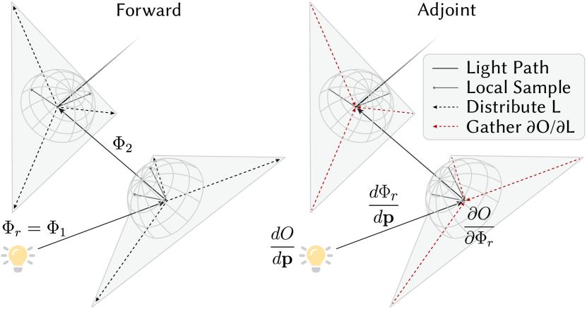
Figure 4. Illustration of our forward and adjoint light tracing approach. In the forward pass we trace radiant flux into the scene, while in the adjoint pass we collect derivatives of the objective function along the light path.

Instead of summing up contributions from all paths to build the full sensitivity matrix $d{L_{klm}}/d\boldsymbol{\mathbf{p}}$, which would consume a lot of memory as the number of parameters grows, we employ an adjoint formulation to compute the gradient of the objective function.

Consequently, instead of tracing derivatives of radiant flux forward along a light path, we instead collect partial objective derivatives (adjoint radiance) backwards along that path and compute a weighted sum of partial derivatives ${\partial O}/{\partial{\Phi_{r}}}$ such that

(11) $$\frac{{dO}}{{d{\mathbf{p}}}}=\sum\nolimits_{r}{\left({\frac{{\partial O}}{{\partial{\Phi_{r}}}}\frac{{d{\Phi_{r}}}}{{d{\mathbf{p}}}}+\frac{{\partial O}}{{\partial f_{1}({{\omega_{o}}})}}\frac{{df_{1}({{\omega_{o}}})}}{{d{\mathbf{p}}}}+\frac{{\partial O}}{{\partial f_{1}({{\omega_{2}}})}}\frac{{df_{1}({{\omega_{2}}})}}{{d{\mathbf{p}}}}}\right)}.$$

The derivative wrt. the BRDF under direct illumination, ${{{\partial O}}/{{\partial f_{1}({{\omega_{o}}})}}}$, only occurs at $\boldsymbol{\mathbf{x}}_{1}$ and can be calculated directly from Eq. ((8) ) and ((6) ). Similarly, the derivative of the BRDF itself wrt. parameters $\boldsymbol{\mathbf{p}}$ follows from the derivative of the BRDF wrt. the angle of incidence and applying the chain rule (again noting that the intersection point $\boldsymbol{\mathbf{x}}_{1}$ remains constant). The other two derivative terms, ${\partial O}/{\partial{\Phi_{r}}}$ and ${\partial O}/{\partial f_{1}({{\omega_{2}}})}$, on the other hand, are adjoint states, collecting objective function derivatives along the light path. We update these terms at every ray-surface intersection point $\boldsymbol{\mathbf{x}}_{i}$, analogous to the forward simulation, Eq. ((8) ):

(12) $$\frac{{\partial O}}{{\partial{\Phi_{r}}}}\leftarrow\frac{{\partial O}}{{\partial{\Phi_{r}}}}+\frac{{\partial O}}{{\partial{L_{klm}}}}\frac{{\partial{L_{klm}}}}{{\partial{\Phi_{i}}}}\frac{{\partial{\Phi_{i}}}}{{\partial{\Phi_{r}}}},$$

and

(13) $$\frac{{\partial O}}{{\partial{f_{1}}({\omega_{2}})}}\leftarrow\frac{{\partial O}}{{\partial{f_{1}}({\omega_{2}})}}+\frac{{\partial O}}{{\partial{L_{klm}}}}\frac{{\partial{L_{klm}}}}{{\partial{\Phi_{i}}}}\frac{{\partial{\Phi_{i}}}}{{\partial{f_{1}}({\omega_{2}})}}.$$

Figure 4 illustrates this idea, which we also outline in Alg. 2.

We find the derivative terms required to evaluate Eq. ((12) ) and ((13) ) as follows: First, ${\partial O/\partial L_{klm}}$ is simply the derivative of Eq. ((6) ), while ${\partial L_{klm}/\partial\Phi_{i}}$ follows from differentiating Eq. ((8) ). Finally, ${\partial\Phi_{i}/\partial\Phi_{r}}$ and ${\partial\Phi_{i}/\partial f_{1}(\omega_{2})}$ are tracked along the light path, effectively expanding the recursive product induced by Eq. ((7) ) and collecting factors.

Algorithm 2 Adjoint light tracing

  Initialize $dO/d\boldsymbol{\mathbf{p}}=0$

  for  each light source with parameters $\boldsymbol{\mathbf{p}}$  do

     for  ray $r\in[1,N]$  do

        Generate exitant ray $(\boldsymbol{\mathbf{x}}_{o},\;\omega_{o})$

        Set $\partial O/\partial\Phi_{r}=0$ and $\partial O/\partial f_{1}(\omega_{2})=0$

        for  $i\in[1,maxBounces]$  do

           Trace ray, find intersection point $(\boldsymbol{\mathbf{x}}_{o},\;\omega_{o})\rightarrow\boldsymbol{\mathbf{x}}_{i}$

           if  $i==1$  then

              Compute $d\Phi_{r}/d\boldsymbol{\mathbf{p}}$ (see §4.4)

              and $df_{1}(\omega_{2})/dp$

           for  $N^{\prime}$ local samples  do

              $\omega_{o}\leftarrow$ uniform random in $\mathcal{H}^{2}$

              for  each vertex $k$ in the triangle containing $\boldsymbol{\mathbf{x}}_{i}$  do

                 for  $l\in[0,n],\;m\in[-l,l]$  do

                    Update adjoint states according to Eq. ((12) )

                    and Eq. ((13) )

           Exitant ray:

           $\boldsymbol{\mathbf{x}}_{o}\leftarrow\boldsymbol{\mathbf{x}}_{i}$

           $\omega_{o}\leftarrow$ $\cos$-weighted random in $\mathcal{H}^{2}$

        Finally, update gradient according to Eq. ((11) ).

4.4. Optimization parameters

Having formulated adjoint states per ray that collect indirect illumination gradients at the first ray-surface intersection, the remaining task is to compute $d\Phi_{r}/d\boldsymbol{\mathbf{p}}$ for the parameters $\boldsymbol{\mathbf{p}}$ of the lighting configuration. The specifics of this term depend on the type of each light source (point, spot, area, etc.) and on the meaning of each parameter (position, intensity, rotation, etc.). These derivatives can generally be calculated analytically, and we briefly summarize them here, while deferring details to the supplementary document.

4.4.1. Intensity and colour

Intensity (per colour channel) ${I_{e}}$ for point-shaped lights (or analogously emissive power for area lights) directly affects the emitted flux per light ray, hence the corresponding derivative is straightforward to calculate. We find it useful to parametrize intensity with a quadratic function, $I_{e}=0.5\boldsymbol{\mathbf{p}}_{j}^{2}$, where $\boldsymbol{\mathbf{p}}_{j}$ is the corresponding optimization parameter, to prevent negative values. If the task is to optimize chromaticity, but maintain a constant intensity, we need to find a colour vector $\boldsymbol{\mathbf{c}}={(r,g,b)}$ such that $r+g+b=1$. We implement this constraint by projecting $\boldsymbol{\mathbf{c}}$ to $\boldsymbol{\mathbf{c}}_{p}=\boldsymbol{\mathbf{c}}/(r+g+b)$ in each optimization step, and similarly projecting the derivative by multiplying with $(d{\mathbf{c}_{p}}/d{{\mathbf{c}}})$.

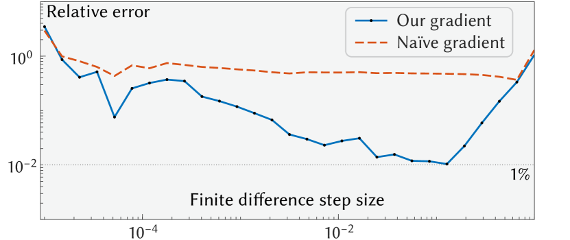
Figure 5. We compare our gradient calculation to a naïve differentiation for the initial configuration shown in Fig. 16. Here we compare the gradient of the objective function wrt. the light’s 3D position to finite difference approximations at various step sizes. Our gradient closely matches FD approximations at intermediate step sizes and we observe the expected trade-off between floating-point errors (too small FD steps) and approximation errors (too large FD steps). The naïve version, however, exhibits systematic errors across a wide range of step sizes.

4.4.2. Position and rotation

Let us now consider the derivative of the objective function with respect to a light’s position $dO/d\boldsymbol{\mathbf{x}}$. The naïve approach would be to assume that each exitant ray is displaced by an infinitesimal perturbation $d\boldsymbol{\mathbf{x}}$ and propagates parallel to the original ray until the first hit $\boldsymbol{\mathbf{x}}_{1}$, and then follows an increasingly perturbed path from there. In this way, we would compute the set of spatial derivatives $d\boldsymbol{\mathbf{x}}_{i}/d\boldsymbol{\mathbf{x}}$. Automatic differentiation would also produce this result.

There is, however, a serious issue with this naïve approach: computing derivatives in this way generally fails to produce descent directions that would be useful for gradient-based optimization of lighting configurations. In a light-tracing approach, the radiance incident on a surface is represented by the discretized distribution of rays intersecting this surface. While path tracing (with next event estimation), or the geometric term in a path-integral formulation, explicitly contain the well-known expression ${(\omega_{1}\cdot\boldsymbol{\mathbf{n}})/r^{2}}$, for light tracing it is instead implicitly encoded into the spatial configuration of rays. However, any spatial derivative of $\boldsymbol{\mathbf{x}}_{i}$ results in a vector in the plane of the triangle containing $\boldsymbol{\mathbf{x}}_{i}$, with discontinuous jumps between triangles, as illustrated in the inset of Fig. 6. As radiant flux is constant along each ray, derivatives wrt.  the light position $\boldsymbol{\mathbf{x}}$ must always be orthogonal to the ray. Rays that intersect a surface near one another are often close to parallel, with only a small angle between them. Consequently, the sum of per-ray derivatives computed in this way suffers from numerical errors and produces a large systematic error in the resulting gradient $dO/d{\mathbf{x}}$, see Fig. 5. These errors prevent a gradient-descent optimizer from converging, even in a very simple problem as shown in Fig. 6.

The PSDR approach [Zhang et al., 2020] avoids this issue by evaluating the entire path according to the path-integral formulation and then applying automatic differentiation (including the explicit geometric term). We take inspiration from this approach, but apply the idea only to the first segment of a path (from $\boldsymbol{\mathbf{x}}_{0}$ to $\boldsymbol{\mathbf{x}}_{1}$), while our adjoint formulation takes care of the indirect illumination path. We also compute the resulting derivative terms analytically with the help of symbolic math tools, rather than code-level AD. Our solution to finding useful gradients wrt. position and rotation of a light source is to consider the “reverse” direction of the primary light ray, $\boldsymbol{\mathbf{x}}_{0}\rightarrow\boldsymbol{\mathbf{x}}_{1}$. Effectively, we compute the derivatives of the direct illumination represented by $\Phi_{r}$ of an arriving ray, as if we were tracing the ray in the other direction (via next event estimation from the scene geometry to the light source). Consequently, we assume that ray-surface intersection points $\boldsymbol{\mathbf{x}}_{i}$ remain constant, even if the light source moves (or rotates).

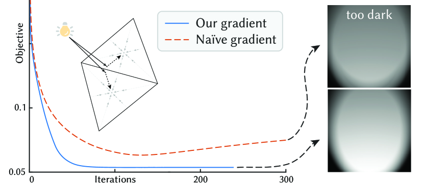
Figure 6. In this example, the goal is to position a spot light such as to find a trade-off between uniformity and a specific brightness on a Lambertian plane. Computing the objective’s gradient using the naïve approach (red dashes) fails to identify the correct distance between the light source and the plane. The inset illustrates how interpolation basis function gradients in the naïve approach push each ray towards the centroid of the intersected triangle, in order to increase brightness equally at all corners. Our method (blue line), in contrast, provides improved gradient information, enabling the optimizer to find the best distance.

We consider a “virtual” intensity per ray, ${{\tilde{I}_{e}}={\Phi_{r}r^{2}/\cos{\omega_{1}}}}$, representing the irradiance this ray transports from the light source to $\boldsymbol{\mathbf{x}}_{1}$: the direct illumination due to $\Phi_{r}$ behaves like ${\tilde{I}_{e}\cos{\omega_{1}}/r^{2}}$ locally. Consequently, the derivative of the incident flux with respect to the light’s position becomes

(14) $$\frac{d\Phi_{r}}{d\boldsymbol{\mathbf{x}}}={\tilde{I}_{e}\;\frac{d(\cos{\omega_{1}}/{r^{2}})}{d\boldsymbol{\mathbf{x}}}}.$$

We compute this derivative using symbolic math software, as shown in our supplementary document. Figure 5 shows relative errors of our gradient, compared to the naïve version discussed earlier, for finite difference (FD) approximations of various step sizes. As expected, for small step sizes finite differencing suffers from floating-point errors, whereas for large step sizes, FD approximation error dominates. For a suitable range of step sizes, our gradients agree well with finite difference approximations. The naïve approach, on the other hand, shows systematic error over a wide range of FD step sizes. This error accumulates during the summation over many rays; for single light paths, we have verified the correct implementation of the naïve gradient calculation.

In Fig. 6 we compare our improved approach to the naïve version on a basic optimization task. The goal is to position a spot light, illuminating a Lambertian plane, to achieve a constant and uniform brightness on the entire plane. Hence, the light must be far enough to cover most of the plane and near enough to provide sufficiently bright illumination. Using our method, gradient descent optimization converges quickly, and reliably remains in the optimal configuration. We intentionally choose a standard gradient descent approach (i.e., updating ${\mathbf{x}}\leftarrow{\mathbf{x}}-\alpha(dO/d{\mathbf{x}})$) instead of more elaborate optimization algorithms for this example, because it most clearly exposes the flaws of the naïve differentiation approach.

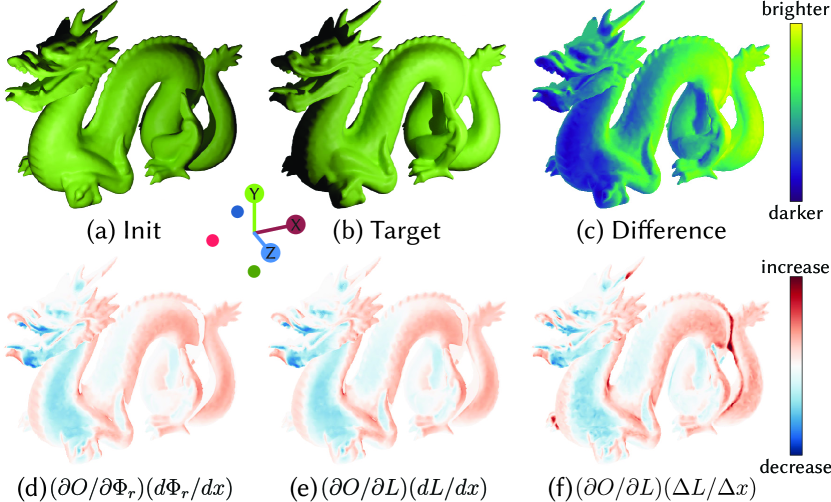
Figure 7. Visualizing gradients on the Stanford Dragon: the top row shows the initial (a) and intended (b) lighting, as well as their difference (c). The second row shows gradient contributions for the $x$ coordinate of a point light using our adjoint approach (d), direct differentiation (e), and a finite difference approximation (f). Image subtitles indicate the calculation; BRDF derivatives are taken into account but not explicitly stated here for brevity.

We parametrize the orientation of light sources by a rotation vector ${\boldsymbol{\mathbf{\theta}}}$, which defines a rotation matrix ${\mathbf{R}(\boldsymbol{\mathbf{\theta}})}$ following Rodrigues’ formula. The world-space orientation (normal $\mathbf{n}$ and tangent $\mathbf{t}$) results from applying this rotation to the material-space normal and tangent $(\boldsymbol{\mathbf{n}}_{0},\boldsymbol{\mathbf{t}}_{0})$ respectively. We use the common linear small-angle approximation to avoid numerical issues when $\|\boldsymbol{\mathbf{\theta}}\|$ approaches zero. Applying the chain rule, we find the derivative of the flux wrt. the rotation vector:

(15) $$\frac{{d{\Phi_{r}}}}{{d{\mathbf{\theta}}}}=\frac{{\partial{\Phi_{r}}}}{{\partial{\mathbf{n}}}}\frac{{d{\mathbf{n}}}}{{d{\mathbf{\theta}}}}+\frac{{\partial{\Phi_{r}}}}{{\partial{\mathbf{t}}}}\frac{{d{\mathbf{t}}}}{{d{\mathbf{\theta}}}},$$

where we compute the terms $d\boldsymbol{\mathbf{n}}/d\boldsymbol{\mathbf{\theta}}$ and $d\boldsymbol{\mathbf{t}}/d\boldsymbol{\mathbf{\theta}}$ using symbolic differentiation of Rodrigues’ formula. Finally, we find ${{\partial\Phi_{r}}/{\partial{\mathbf{n}}}}$ and ${{\partial\Phi_{r}}/{\partial{\mathbf{t}}}}$ via symbolic differentiation, again keeping $\boldsymbol{\mathbf{x}}_{1}$ fixed. The exact expressions depend on the type of light source. For instance, IES data files [ANSI/IES, 2020]—which are widely used in architecture—define the emitted intensity by tabulated values, interpolated bilinearly over the unit sphere; spot lights with soft edges use a quadratic attenuation profile between the inner and outer cone angle; whereas area light sources assume a cosine-weighted emission profile. Please refer to our supplementary document for further details. Note that for area lights the ray origin moves when the light is rotated, i.e., ${\boldsymbol{\mathbf{x}}_{0}(\boldsymbol{\mathbf{\theta}})}$. (For our purposes we only consider rigid rotation and translation.) In this case, the derivatives wrt. the light’s orientation include an additional term, analogous to Eq. ((14) ) to account for the shift of the ray origin, as described in the supplement.

4.4.3. Further parameters

Because Eq. ((11) ) separates derivatives of the objective function from derivatives of the lighting configuration, we can in principle extend our optimization system to include other parameters relatively easily. The main question we have to address for each parameter, is how it affects the incident radiance (discretized using many rays) at the first ray-surface intersection, thereby formulating derivatives of each ray’s radiant flux, such as to represent the expected change in the direct illumination. In general, we believe this idea of including knowledge about a global behaviour into local, but discretized, derivative calculations could also be beneficial for other applications.

5. Visualizing gradient contributions

In common camera-based differentiable rendering, the gradient of the rendered image with respect to a specific parameter can be visualized as a gradient image [Zhang et al., 2020; Zeltner et al., 2021], or a gradient texture [Nimier-David et al., 2020; Zeltner et al., 2021] when optimizing an object’s appearance. Our method, however, computes the full radiance field instead of a single image. During optimization, we employ an adjoint formulation that avoids computing derivatives of this radiance field explicitly. We can compute these derivatives for visualization and comparison, but more interestingly, we can also use our per-ray adjoint states for a different kind of visualization showing adjoint gradient contributions as follows.

For any point $\boldsymbol{\mathbf{q}}$ on the surface geometry (that is directly visible from a selected light source), we can construct a light path that originates at that light and passes through $\boldsymbol{\mathbf{q}}$ as its first ray-surface intersection, and then continues bouncing through the scene. Evaluating Eq. ((11) ) for these paths only, we find contributions to the derivative $dO/d\boldsymbol{\mathbf{p}}_{j}$ that “flow” through the point $\boldsymbol{\mathbf{q}}$. Intuitively, we can think of each point $\boldsymbol{\mathbf{q}}$ casting a vote on how the parameter $\boldsymbol{\mathbf{p}}_{j}$ should change in order to improve the objective function (while taking indirect reflections from $\boldsymbol{\mathbf{q}}$ into account). Note that this quantity is different from adjoint radiance [Nimier-David et al., 2020], which does not include derivatives wrt. parameters, or indirect bounces.

The example in Fig. 7 shows which parts of the dragon would improve the objective function if the light moves right (red) or left (blue). The final objective function gradient $dO/d\boldsymbol{\mathbf{p}}$ can be thought of as the sum of these contributions. We also compare our visualization to a reference implementation that directly differentiates the radiance field and a finite difference approximation. For (mostly) direct lighting, our method and the reference yield nearly identical results (both implementations ignore discontinuous integrands for comparison, while FD approximation diverges at these discontinuities, but matches the other results well overall). In our supplementary material, we also show a situation where the objective is strongly influenced by indirect illumination, where our adjoint visualization draws gradient contributions at the first ray-surface intersection, whereas direct differentiation produces a response at the target surface.

6. Results

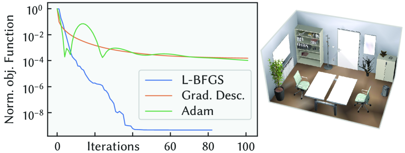
Figure 8. Optimizing the intensities of 10 point lights to recover a ground-truth illumination. The inset image shows the L-BFGS result in form of our radiance cache, which is visually indistinguishable from the ground truth. Step sizes are $\alpha=10$ for ADAM and $\alpha=0.01$ for gradient descent.

In this section we present results obtained with our method, first covering verification test cases, as well as comparisons to related methods. Finally, we demonstrate the ability of our approach to address creative lighting design cases. Unless stated otherwise, we trace two indirect bounces in all of our results. Our implementation can either be used standalone (optionally with a graphical user interface providing real-time feedback) or via a Python interface. All our light transport simulations run on the GPU, specifically a NVIDIA GeForce RTX 3080, using the Vulkan Graphics API in combination with hardware-accelerated ray tracing. We also evaluate the objective function on the GPU, but transfer the optimization parameters and their derivatives to the CPU, in order to access publicly available optimization libraries. Running the optimization algorithm on the CPU is not a performance bottleneck, as the size of the parameter vector is much smaller than the size of the radiance data.

In general, it is difficult to predict which optimization algorithm will perform best for each specific task. Our results show that we provide gradient information that works with many commonly used optimization methods. Our implementation uses the LBFGS++ library [2021], as well as the ADAM algorithm of Kingma and Ba [2014] (using decay rates $\beta_{1}=0.9$ and $\beta_{2}=0.999$ as suggested in the original publication for all our results). For comparisons to gradient-free CMA-ES, we use the code by Hansen [2003; 2021]. We perform high-quality rendering using our own physically based (non-differentiable) path tracer, but also show direct visualizations of the radiance data we use for optimization.

6.1. Verification tests

We first consider some basic test cases to verify that our differentiable light-tracing system is capable of solving various inverse problems where a well-defined solution is available for comparison.

In Fig. 8 we show a ground-truth recovery test performed with different optimization algorithms, all of which use our gradients as input. In this test, we place 10 point lights in a regular $5\times 2$ grid pattern and set their power to $40$ W each. The task is to find the ground-truth illumination, which is defined by only one specific light at $200$ W. We compare gradient descent (GD), ADAM [Kingma and Ba, 2014], and L-BFGS [Nocedal, 1980] on this task of “selecting” the correct light source. The other lights introduce local minima separated by saddle points, consequently GD and ADAM converge very slowly as they approach a saddle. This test shows the importance of providing not only accurate gradient information, but also objective function values, which allow L-BFGS (or other quasi-Newton optimization methods) to estimate the step length and evaluate Wolfe conditions during line search. Note that in our other results, ADAM is often successful in finding a good solution. Therefore, we implement our method such that objective function value and gradient can always be provided, which allows us to easily extend our system with any first-order optimization algorithm if needed. Conversely, if we were to only provide gradient estimates based on sub-sampled data, as is often done when using stochastic GD or stochastic ADAM, we might not be able to obtain good convergence behaviour on complex optimization tasks, as evidenced in Fig. 8. We perform a similar ground-truth test for a glossy coin, using hemi-spherical harmonics up to order $n=5$, in Fig. 9. Please also refer to our supplementary material for a visual comparison of different orders of HSH interpolation, which shows that our radiance data structure converges under refinement.

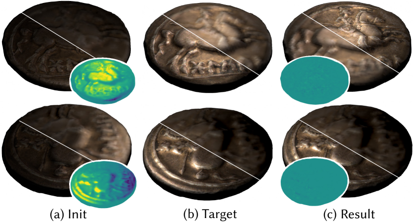
Figure 9. Recovering the ground-truth position of a point light illuminating a glossy coin. initial lighting (a), the target (b), and our result (c) with the insets showing their differences to the target. Top row: front view, second row: side view. The top-right parts (a, b, c) show our data structure, while the bottom-left shows a high-quality rendering of the same lighting configuration.

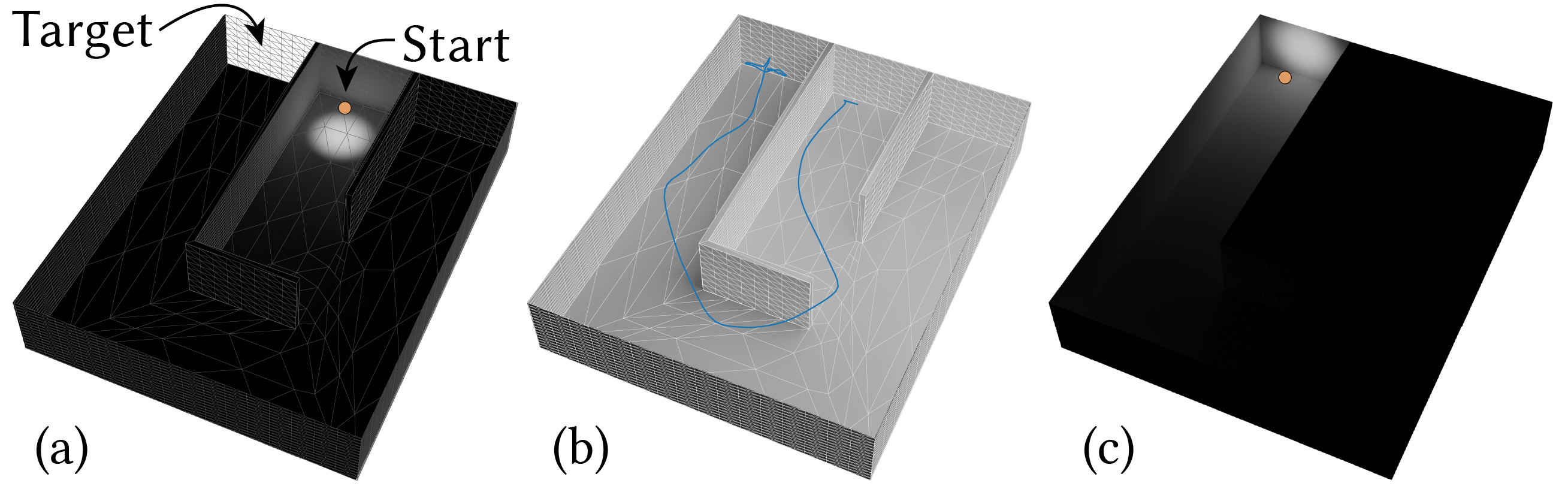
Figure 10. Optimizing with indirect illumination: a spot light starts in the middle hallway of a simple labyrinth (a) and the target (overlaid on the far left wall) is only illuminated very dimly by indirect light. The ADAM optimizer simultaneously rotates and translates the light source around the corners (b) to find the “exit” (c).

Finally, we test the capabilities of our system in dealing with indirect illumination, Fig. 10. We place a spot light into a small “labyrinth”, such that light can only reach the “exit” via multiple bounces. The side walls of the labyrinth have a dark target value to push the light away from the walls, with a very low weight ($\alpha_{k}=0.004$), whereas the exit has a very bright target with unit weight to attract the light source. We trace light paths with $10$ indirect bounces in this example. Optimizing for position and rotation simultaneously using ADAM with step size $\alpha=0.2$ successfully navigates the light through the labyrinth in ca. $10$ s and $200$ gradient evaluations. In principle, L-BFGS also successfully solves this problem, but the momentum estimated by ADAM results in a smoother, visually appealing motion of the light source.

6.2. Comparison to previous work

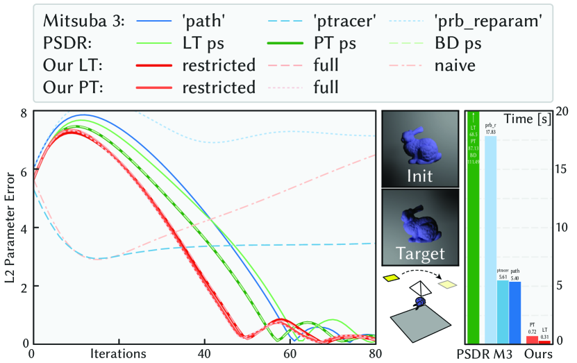
Figure 11. A baseline comparison on a simple test scene, moving an area light to a ground-truth position (inset images), showing the convergence of our method, PSDR and Mitsuba 3 in terms of parameter-space distance. All methods run ADAM with step size $\alpha=0.25$, $4$ indirect illumination bounces and $1$ million samples. On this simple scene, restricting our objective function to visible surfaces (’restricted’) results in the same convergence rate as using the entire radiance data (’full’). Note that Mitsuba’s ’prb_reparam’ method eventually converges (around $150$ iterations), whereas their ’ptracer’ does not. The graph on the right shows the total runtime for $80$ iterations: our light tracer is about twice as fast as our reference path tracer, while comparing the three Mitsuba integrators shows the runtime impact of discontinuity handling.

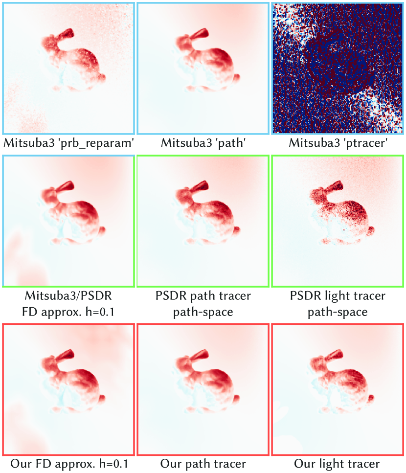
Figure 12. Gradient images wrt. the $x$ coordinate of the area light for the initial state in Fig. 6.2; colour range: $-0.05$ (blue) to $+0.05$ (red). We compute $16$ million total samples for each image. Mitsuba 3’s particle tracer fails to produce correct results. PSDR’s path-space approach works, but light tracing causes higher noise than their path tracer. Note that Mitsuba’s ’prb_reparam’ integrator is the only method that resolves the gradient in the drop shadow correctly compared to finite difference approximation. Note that our adjoint light tracer visualizes indirect gradient contributions differently than our path tracer, see §5 for a detailed explanation.

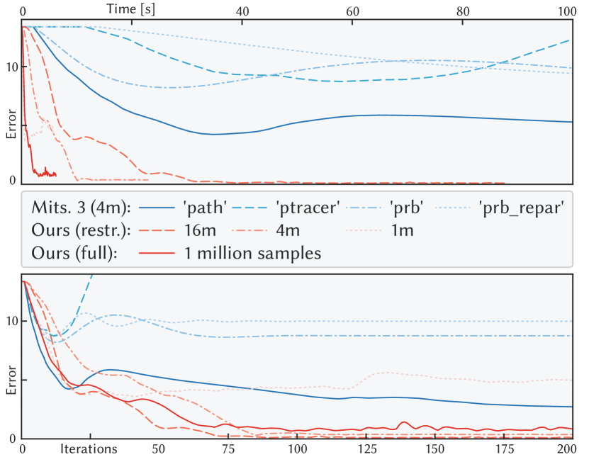
Figure 13. Runtime (top) and convergence (bottom) comparisons of our method with Mitsuba 3 on the same scene as shown in Fig. 1 modified with four cameras and four lights sources. We show results for a restricted version of our method consisting only of camera-visible data (see Fig. 14), as well as a full version. Four different integrators of Mitsuba 3 were used and all Mitsuba 3 tests were done with $4$ million samples, while for our algorithm we chose 1, 4, and 16 million samples. The error is the Euclidean distance between current and target light positions and intensities in parameter space. Note that our full version with just 1 million samples performs similar to our restricted version using 4 times the amount of samples.

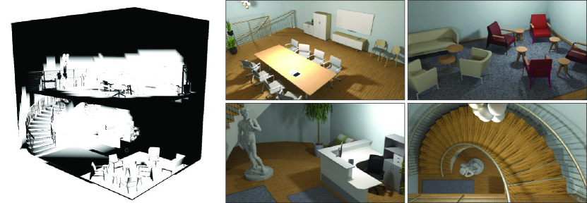
Figure 14. Objective function weights for the comparison in Fig. 13: we restrict our objective by weighting the contribution of vertices (left, white: $\alpha_{k}=1$, black: $\alpha_{k}=0$) based on their visibility to the cameras used by Mitsuba. The camera views used when optimizing with Mitsuba are shown on the right.

Current work on inverse rendering always considers images to define the optimization objective. We establish a baseline for comparing our view-independent approach to existing methods by restricting our objective function to data available in image-based methods (camera-visible surfaces only) on a simple test scene, where one camera sufficiently captures most surfaces (except of course the back of the bunny). In this test, we use ideally diffuse materials for all objects in the scene to allow for a fair comparison. As shown in Fig. 6.2, our adjoint light tracing matches state-of-the-art methods in this setting in terms of optimization convergence, while our adjoint formulation, combined with an efficient GPU-based implementation outperforms other methods in terms of runtime. Mitsuba’s light tracing method (’ptracer’), using automatic differentiation, fails to converge, similarly to our naïve differentiation approach (described in §4.4.2). The differentiable path-integral formulation of PSDR [Zhang et al., 2020], on the other hand, produces good results in this simple setting for both light (’particle’) and path tracing (with slightly more noise and reduced convergence rate of their light tracer). While related image-based methods (Mitsuba, PSDR) handle discontinous edges in various ways, one interesting observation in our tests (Fig. 6.2) is that Mitsuba’s reparametrized path-replay backpropagation (’prb_reparam’) is the only existing method that correctly resolves the gradient near the drop shadow of the Bunny. However, it also introduces noise into the gradient, causing reduced optimization convergence (Fig. 6.2). As discontinuity handling also comes with a runtime cost, we choose speed over (theoretical) accuracy in our method and leave view-independent treatment of discontinuities as future work. Note that our adjoint visualization in Fig. 6.2 shows gradient contributions of indirect lighting differently to common approaches, as detailed in §5 and our supplement. Overall, our approach produces less noisy gradient data compared to existing differentiable light tracing methods.

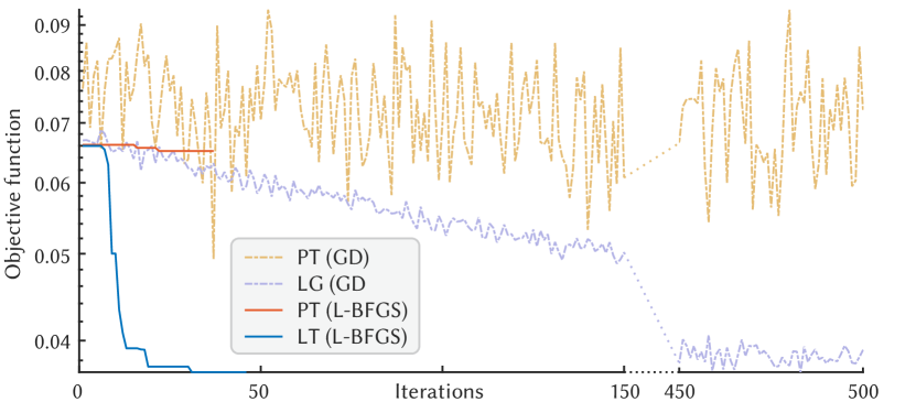
Figure 15. Equal-time comparison between our adjoint light tracing and our reference differentiable path tracing implementation on the combined optimization of the light source’s position and intensity, as in Fig. 16. Using our gradients, both gradient descent (step size $\alpha=0.1$) and L-BFGS converge robustly, whereas differentiable path tracing produces more noisy gradients, preventing convergence. (Note that we squeeze the x-axis between iterations $150-450$ to show the later gradient descent iterations. L-BFGS, on the other hand, terminates when it fails to find an improved configuration.)

For further comparison, we also implement a reference differentiable path tracer (without discontinuity handling) following the ideas of Stam [2020] on top of our view-independent data structure. We uniformly sample each triangle, similar to samples per pixel for camera-based rendering, and trace paths with next event estimation to find the incident radiance. Finally, we sample exitant directions locally, apply the BRDF and update our data structure according to Eq. ((8) ). This path tracer uses the same sampling strategies to construct indirect illumination paths as our light tracer for a fair comparison. In this way, we compare our light tracing method against “object-space” path tracing; the gradients produced by this path tracer closely match Mitsuba’s AD path tracer and PSDR’s path tracer (Fig. 6.2). In our simple test scene, optimization convergence (Fig. 6.2) is nearly identical between our light tracer and the reference path tracer (though our light tracer has a runtime advantage).

For the baseline test scene we observe similar results between restricted objective function data and full view-independent data (i.e., camera-visible vs. all surfaces in the scene), as intended. We show an extension of this test scene in our supplement, where adding an off-camera box around the scene highlights the advantage of a view-independent approach.

Our reference path tracer also achieves convergence similar to our light tracer on the intensity optimization test (Fig. 8). However, in equal-time comparisons on more complex scenes and optimization problems, such as the combined position and intensity test (Fig. 16), our light-tracing method yields improved convergence rates, as shown in Fig. 15, due to reduced (gradient) noise (see also the indirect illumination "labyrinth" example in our video).

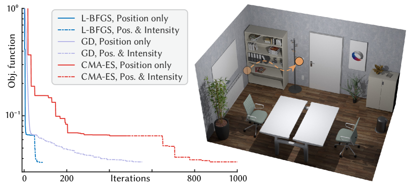
Figure 16. A basic lighting design case: the image shows initial and optimal light position (according to the target shown in Fig. 17b) overlaid on the final illumination. The light becomes brighter and moves centrally over the tables during optimization. We compare convergence of gradient descent and L-BFGS (both using our gradients) to gradient-free CMA-ES optimization (initial standard deviation $\sigma=1$ for all parameters). With each method, we first optimize only the light’s 3D position (solid lines) and then its position and intensity combined (dashed lines).

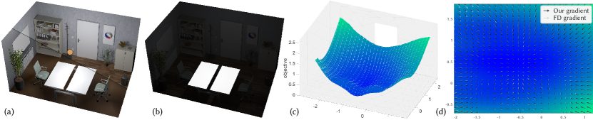
Figure 17. Further analysis of the design case shown in Fig. 16: image (a) shows the result after optimizing only for the light position, the upper part shows the high-quality rendered result, the lower part previews our radiance data structure used for optimization; (b) the target requires the tables to be lit uniformly (the rest of the scene has zero weights and does not affect the objective). We evaluate the objective on a regular grid and plot the result (c), the background shows the mesh of the floor and far walls for context. Arrows show negative gradients wrt. $(x,z)$-position of the light, which reliably point towards a local minimum. We visually compare these gradients to a finite difference approximation (d).

Finally, we compare our approach to Mitsuba 3 on a large scene, where Mitsuba uses four cameras to cover most of the scene. We again restrict our method to surfaces visible by any camera for comparison. Mitsuba’s reparmetrization shows reduced optimization performance, while using our method without restriction to visible surface improves convergence, even at lower sample count. We believe this behaviour is due to the global coupling between parameters in the lighting design problem, where discontinuous edges have less influence than the correlation between parameters in terms of the resulting global illumination effects. In this way, the lighting design problem is a significantly harder optimization problem than, for instance, optimizing texture colours given a target image.

In summary, our adjoint light tracing method at least matches, and on complex scenes outperforms, state-of-the art inverse rendering on the lighting design problem, and enables a fast GPU implementation. We intentionally ignore discontinuities, which does not impact optimization performance due to the global nature of lighting optimization. Additionally, we also allow for visualizing adjoint gradient contributions, including indirect illumination. Overall, we consider our adjoint light tracing method a useful contribution to the growing differentiable rendering toolbox.

6.3. Lighting design applications

6.3.1. Small office lighting

We first show an example of a fully automatic optimization of a single point light in a small office scene, Fig. 16 and 17. The optimization target (Fig. 17b) specifies bright, but uniform lighting on the top surface of both tables, a common regulatory requirement for work spaces. In the initial configuration, a point light (transparent orange dot in Fig. 16) is placed off to one side, causing the work space to be too dimly and unevenly lit. We test different optimization methods on two subsequent tasks on this scene. We first optimize only for the 3D position of the light, which moves to a location centrally above the tables, finding a good trade-off between brightness and uniformity (Fig. 17a). Afterwards, we jointly optimize for the light’s intensity and position. The optimal light placement is now just underneath the ceiling, still centrally over the tables (thereby improving uniformity), with the intensity increased to compensate for the larger distance.

We compare the performance of GD and L-BFGS to a gradient-free CMA-ES approach [Hansen et al., 2003] in Fig. 16. In the first, position-only, optimization task, both L-BFGS and GD reliably find a good solution in $6.5~{}s$ and $42$ objective and gradient evaluations, or $7.9~{}s$ and $52$ evaluations respectively. In comparison, the gradient-free CMA method requires around $200$ objective evaluations to find a good solution. In general, the computation time required to evaluate gradients via an adjoint method is close to the time needed to compute the solution itself. See also Table 1 for timings of the forward and adjoint evaluations in our examples. Therefore, even though CMA-ES does not need to evaluate gradients, the total runtime is still significantly slower than gradient-based methods. In the second task, when we optimize for position and intensity simultaneously, the Hessian approximation built by the L-BFGS method captures the relation between the height (distance) and intensity. Consquently, L-BFGS finds a good solution (Fig. 16) in $8.2~{}s$ and $45$ evaluations. Plain gradient descent, on the other hand, converges more slowly, while CMA finds an acceptable solution after about $400$ evaluations.

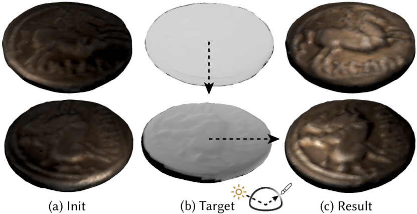
Figure 18. Lighting an ancient coin according to a user-defined directional lighting target (top row: front view, bottom row: side view). Initially the light source is positioned on the left side of the coin (a) when viewed from the front. The user-defined target (b) describes a illumination configuration which is more optimal for this front view, resulting in a significant improvement (c) over the initial state.

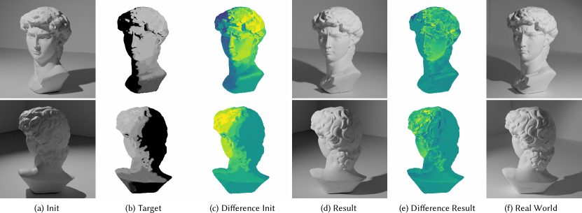
Figure 19. Lighting design study on the bust of David: we first generate a flat initial lighting of the laser-scanned model (a), then sketch a desired side lighting in 3D (b) and optimize the position and rotation of the point light source to match this target (d). We then re-create the optimized lighting setup using the real-world specimen (f). Columns (c) and (e) show the difference to the target before and after optimization respectively.

6.3.2. Directional lighting of a glossy coin

In Fig. 18 we show an example where directional lighting plays an important role. The user specifies a direction-dependent target by painting directly into the HSH-discretized data structure and coefficients ${L_{klm}^{*}}$. In this example, we set the per-channel weights $\alpha_{l}$ such as to under-weight the undirected lighting component represented by $H_{0}^{0}$ by a factor of $0.1$ relative to the directional components of the radiance data. Using our adjoint gradients, an L-BFGS optimizer successfully navigates the light source around the coin to find the best matching directional lighting configuration.

6.3.3. Real-world bust of David

Here, we demonstrate the applicability of our system to an artistic lighting design process on a small bust of David figurine. We first laser-scan the bust and build a 3D mesh suitable for our simulation using a Metris MCA 3600 articulated arm with a Metris MMD50 laser scanner. In our interactive user interface, we then sketch a desired shading onto this model. Performing $100$ iterations of ADAM optimization ($\alpha=0.14$), which takes about $7.5$ s, we find the position and orientation of a spot light that matches the painted target as closely as possible. In order to validate our result, we replicate this lighting configuration on the real-life specimen, Fig. 19. We use a Cree® XLamp® CXA1304 LED and a custom-made snout to limit the cone angle to $45\degree$, matching our simulation. We apply only basic white balance and gradation curve adjustments to the real-world photographs. Overall, the lighting on the real-world specimen closely matches our optimized design.

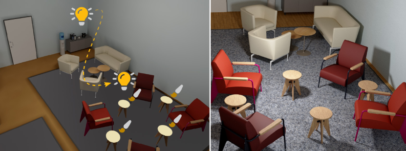
Figure 20. Iterative refinement of the scene shown in Fig. 1. First, desired changes are sketched on the 3D geometry (left), then the optimization adjusts the nearest light’s position accordingly (right).

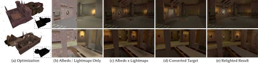
Figure 21. Recovering light parameters for relighting an old PC game which originally shipped with baked lighting only: the original “look” of the game (c) is produced by combining albedo textures and lightmaps (b). From this data, we construct an optimization target (d) and use it to find a new lighting configuration (e) as close as possible to the original (c). Our optimization starts from a regular grid layout of lights and finds a suitable arrangement for them (a). Ultimately, this enables relighting old games often missing dedicated lights with more advanced rendering techniques (e.g., ray-tracing).

6.3.4. Refurbishing baked lighting

Another interesting application of our system is “refurbishing” old video games. In many cases, the diffuse (potentially also indirect) illumination is baked into static lightmaps. However, all information about the original light sources, which would be required to render the scenes with a modern rendering algorithm (e.g., real-time path tracing) is often lost. Here, we reconstruct light sources such that the given textures (which we assume to represent albedo) combined with the recovered lighting produce a similar impression as the original game. We demonstrate this approach in Fig. 21, where we build lighting configurations for two different scenes. In each case, we first initialize a regular horizontal grid of low-intensity point lights, covering the bounding box of the scene. We then perform multiple optimization passes: first, we optimize for position, colour, and intensity of all lights simultaneously using ADAM with a step size $\alpha=0.1$. We refine the result using three L-BFGS passes: the first and third pass optimize for colours and intensities of all lights, while the second pass operates on their positions only. Figure 21 shows overviews of the initial and final lighting configuration, as well as interior views of our results.

6.3.5. Large office (teaser)

In a more complex example, we show a lighting optimization of a large office consisting of two floors. This scene is illuminated by two point lights (one over the staircase, one over the lounge area), two spot lights near the reception and statue, an area light over the conference table, and two highly anisotropic lights (using IES intensity profiles [ANSI/IES, 2020]) on the top floor. Please also refer to our accompanying video for a visualization of this lighting setup. We first show a result that recovers a given ground-truth (Fig. 1). We also compare our method to Mitsuba 3 on this scene (replacing the IES lights, which are not supported by Mitsuba, with spot lights) in §6.2. We then demonstrate the ability of our system to interactively edit the desired illumination and automatically reconfigure the lighting design accordingly in Fig. 20.

6.3.6. Theatre stage lighting

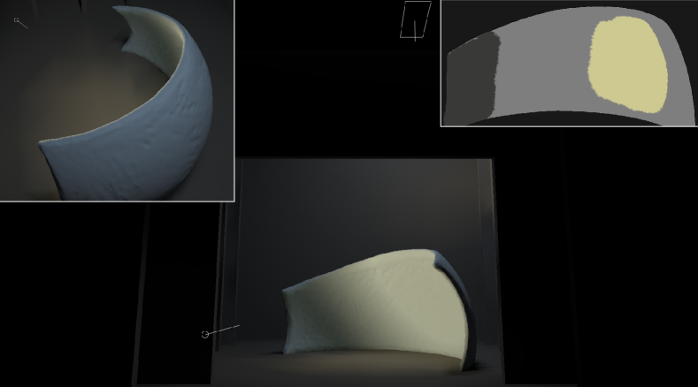
Figure 22. Lighting a theatre stage; please also refer to our accompanying video for the design interaction. The main image shows the audience view, illuminated by a spot light on the left and an area light on top. The inset on the left shows a top-down view of the stage. The inset on the right shows a part of the user-drawn lighting target.

Finally, we show an interactive design session, where the user starts from a completely unlit scene and iteratively adds light sources, selects optimization parameters, and updates the illumination target. The interactive workflow alternates between user manipulations and automatic lighting optimization to realize the intended design, as shown in our video. Figure 22 summarizes the result of this design example. In total, this lighting design session required about $10$ minutes to complete, with just over $2$ minutes spent on automatic design optimization, and the remaining time on various user interactions including visual inspection of the results. Please also refer to Table 1 for a performance overview of our results.

7. Conclusion and Limitations

To our knowledge, this paper presents the first view-independent differentiable light-tracing global illumination solver. Our adjoint light-tracing method efficiently computes reliable gradients, allowing for fast and interactive first-order optimization of lighting designs. We also provide a novel visualization of adjoint gradient contributions to help the user understand the composition of the objective function gradient. Our validation tests show that differentiating the incident flux, while keeping the first ray-surface intersection point constant, captures gradients of information that is contained in the distribution of discrete light rays. Our method computes more accurate gradients compared to a naïve approach as evidenced by finite difference and optimization convergence tests. We also show that (in equal time comparisons) adjoint light tracing results in improved optimization convergence behaviour than differentiable path tracing. Furthermore, we show the applicability of our system to various lighting design tasks, including work spaces, artistic installations, and video game refurbishing.

Table 1. Overview of our results. Columns: scene reference, optimization algorithm, step size $\alpha$, number of primary rays (threads) $N$, number of mesh vertices $m$, average time per forward and adjoint evaluation $t_{L}$, $t_{\nabla}$ [ms], total wall clock time for the entire optimization $t$ [s].

Scene (Fig.)	Optim.	$\alpha$	$N$; $m$	$t_{L}$; $t_{\nabla}$	$t$
Large Office (1)	ADAM	0.1	2.9e7	310	63.0
			1 409 381	306
Small Office (8)	L-BFGS	1	1.0e7	375	35.9
(intensities)			301 009	36
Coin (9)	L-BFGS	1	4.2e6	147	18.4
(HSH $n=5$)			6 345	174
Labyrinth (10)	ADAM	0.2	1.0e6	31	10.8
			1 893	22
Labyrinth	ADAM	0.2	2.4e6	35	9.5
(path trace - video)			1 893	12
Small Office (16)	L-BFGS	1	4.2e6	152	14.7
			301 009	28
Small Office (15)	L-BFGS	1	7.5e7	127	13.5
(path trace)			301 009	62
Small Office	L-BFGS	1	4.2e6	673	16.2
(HSH $n=3$)			301 009	61
David (19)	ADAM	0.14	4.2e6	28	6.8
			535 071	37
Coin painted (18)	L-BFGS	1	4.2e6	123	22.5
(HSH $n=5$)			6 345	154
Game (21 top)	ADAM	0.1	5.1e7	497	80.8
			16 414	293
Dragon (video)	ADAM	0.1	3.6e7	20	18.8
			25 000	72
Theatre stage (22)	L-BFGS	1	1.8e7	97	67.6
(5x L-B. + 1x A.)	ADAM	0.2	38 448	202	60.6

We focus on continuous optimization of a given lighting configuration, relying on the user to provide an initial placement of light sources, either interactively or as part of the original scene description. In the future we will investigate extending our method with mixed-integer optimization approaches to also optimize for non-continuous parameters like the selection of light sources. Currently, we do not handle discontinuities at feature edges in our derivatives, as has been done in previous work on camera-based differentiable rendering. Because our lighting objectives measure relatively large areas and our radiance solution is continuously interpolated, our method converges robustly nonetheless. In the future, it will be interesting to investigate discontinuity handling for specific applications, such as lampshade design, that rely on accurately placing an occluding object in front of a light source. In our implementation, we do not employ advanced sampling strategies, like importance sampling, which are often used to increase the efficiency of Monte Carlo methods. Such methods have recently been successfully applied to differentiable image rendering. As the resulting methods may require parameter-dependent sampling, thereby complicating the calculation of derivatives, we leave this line of research in the context of our light-tracing approach for future work. Similarly, we currently use a user-defined number of HSH basis functions to represent the directional component of the radiance field. In the future it could be interesting to investigate choosing the interpolation order adaptively based on the material properties and lighting conditions. We use piece-wise linear interpolation on triangle meshes, which is easy to understand and implement, but other interpolation spaces, such as (bilinear) texture mapping could be used as well and would fit into our theoretical framework directly.

In conclusion, we have shown that our adjoint light tracing method enables continuous, gradient-based optimization for various lighting design tasks. Providing objective function values and gradients in each iteration allows us to use any first-order optimizer in black-box fashion. Potential applications range from finding optimal work space lighting, to refurbishing old video games, as well as supporting an interactive artistic lighting design process as evidenced by our various results. We have also shown that view-independent optimization enables applications that cannot be easily handled by state-of-the-art image-based inverse rendering. Continuous view-independent optimization is only the first step—we believe our approach opens up a number of interesting directions for future research.

Supplementary material

Supplementary material

(Hemi-) Spherical Harmonics

The spherical harmonics (eigenfunctions of the Laplacian on the unit sphere, see also [Green, 2003; Wieczorek and Meschede, 2018]) are defined as

(S.1) $$Y_{l}^{m}(\varphi,\theta)=\left\{{\begin{array}[]{*{20}{l}}{K_{l}^{m}P_{l}^{-m}(\cos\theta)\sqrt{2}\sin(-m\varphi),}&{m<0}\\ {K_{l}^{m}P_{l}^{m}(\cos\theta),}&{m=0}\\ {K_{l}^{m}P_{l}^{m}(\cos\theta)\sqrt{2}\cos(m\varphi),}&{m>0}\end{array}}\right.$$

where $\varphi$ is the azimuth angle, $\theta\in[0,\pi]$ is the elevation angle, and the scaling factors are

(S.2) $$K_{l}^{m}=\sqrt{{{(2l+1)}}\frac{{(l-\left|m\right|)!}}{{(l+\left|m\right|)!}}}.$$

The associated Legendre polynomials $P_{l}^{m}$ are commonly written as recurrence relations (Green [2003] also provides code for evaluating them):

(S.3) $$\begin{gathered}(l-m)P_{l}^{m}(x)=x(2l-1)P_{l-1}^{m}(x)-(l+m-1)P_{l-2}^{m}(x),\hfill\\ P_{m}^{m}(x)={(-1)^{m}}(2m-1)!!{(1-{x^{2}})^{m/2}},\hfill\\ P_{m+1}^{m}(x)=x(2m+1)P_{m}^{m}(x).\hfill\\ \end{gathered}$$

The hemispherical harmonics $H_{l}^{m}$ are eigenfunctions of the Laplacian on the unit hemisphere. They are defined in almost the same way as $Y_{l}^{m}$ (see also [Gautron et al., 2004]), except that the elevation angle is limited to the range $[0,\pi/2]$, and the associated Legendre polynomials are evaluated for the argument ${(2\cos\theta-1)}$ instead of ${(\cos\theta)}$. The local coordinate system $(\varphi,\theta)$ is oriented according to the surface normal and tangent.

Derivation of the radiance cache update rule

In this section, we summarize the derivation of the update rule presented in the main paper as Eq. ((8) ). First, note the following properties of our spatial and directional interpolation basis functions $\varphi$ and $H_{m}^{l}$, namely nodal Kronecker and partition of unity spatially, and $2\pi$-orthonormality for the hemispherical harmonics:

(S.4) $${\varphi_{k}}({{\mathbf{x}}_{j}})={\delta_{jk}},\quad\sum\nolimits_{k}{{\varphi_{k}}({\mathbf{x}})}=1,$$

(S.5) $$\int_{{\mathcal{H}^{2}}}{H_{m}^{l}(\omega)H_{m^{\prime}}^{l^{\prime}}(\omega)\;d\omega=2\pi{\delta_{mm^{\prime}}}{\delta_{ll^{\prime}}},\quad H_{0}^{0}=1}.$$

Figure S1. Convergence of our spatio-directional radiance data structure with increasing order of the hemi-spherical harmonic basis: top row shows a high-quality rendering (left) and a result without any directional data (i.e. $n=0$). The left column shows a close-up of the region indicated by the yellow rectangle with per-vertex HSH functions visualized on small hemispheres. The last row shows the result after applying two LS3 [Boyé et al., 2010] subdivision steps to all triangles.

Assume, for now, an a-priori known radiance field ${L(\boldsymbol{\mathbf{x}},\omega_{o})}$, which we discretize according to Eq. ((4) ) and ((5) ), i.e. we aim to find the coefficients $L_{klm}$ best approximating this field. In the spatial domain, we determine the local directional functions ${L_{k}}({\omega_{o}})$ in Eq. ((4) ) via $L_{2}$-projection with mass lumping, in line with a finite element analysis [Larson and Bengzon, 2013]. $L_{2}$-projection of a function $f$ to its approximation $f_{h}$ is defined by $\int{(f-{f_{h}}){\varphi_{k}}\;d{\mathbf{x}}}=0$. Applying this definition to the radiance field and discrete approximation, Eq. ((4) ), yields $\int_{\Omega}{L({\mathbf{x}},{\omega_{o}}){\varphi_{k}}({\mathbf{x}})\;d{\mathbf{x}}}=\int_{\Omega}{\sum\nolimits_{j}{{\varphi_{j}}({\mathbf{x}})}{L_{j}}({\omega_{o}}){\varphi_{k}}\;d{\mathbf{x}}}$. Mass lumping then identifies $L_{j}$ with $L_{k}$, and by partition of unity the right-hand side simplifies to ${L_{k}}({\omega_{o}})\int_{\Omega}{{\varphi_{k}}({\mathbf{x}})d{\mathbf{x}}}={{L_{k}}({\omega_{o}})A_{k}}$. Consequently, we find

(S.6) $${L_{k}}({\omega_{o}})=\frac{1}{{{A_{k}}}}\int_{{\Omega_{k}}}{{\varphi_{k}}({\mathbf{x}})L({\mathbf{x}},{\omega_{o}})\;d{\mathbf{x}}},$$

where we integrate over the one-ring neighbourhood ${\Omega_{k}}$ of vertex $k$ (i.e. the support region of the shape function $\varphi_{k}$), and $A_{k}=|{\Omega_{k}}|/3$ is the vertex-associated area. Intuitively, Eq. ((S.6) ) computes the area-weighted average of the exitant radiance around each vertex.

In the directional domain, we follow the same idea, applying $L_{2}$-projection over the hemisphere $H^{2}$: $\int_{{H^{2}}}{{L_{k}}({\omega_{o}})H_{m^{\prime}}^{l^{\prime}}({\omega_{o}})\;d{\omega_{o}}}=\sum\nolimits_{lm}{{L_{klm}}}\int_{{H^{2}}}{H_{m}^{l}({\omega_{o}})H_{m^{\prime}}^{l^{\prime}}({\omega_{o}})\;d{\omega_{o}}}$. We then take advantage of the orthogonality of the hemi-spherical harmonic basis functions to determine the coefficients of our solution:

(S.7) $${L_{klm}}=\frac{1}{{2\pi}}\int_{{\mathcal{H}^{2}}}{H_{m}^{l}({\omega_{o}})\;{L_{k}}({\omega_{o}})\;d{\omega_{o}}}.$$

Consequently, the projection operator for a given radiance field onto our disretize data structure is

(S.8) $${L_{klm}}=\frac{1}{{{A_{k}}}}\frac{1}{{2\pi}}\int_{{\Omega_{k}}}{\int_{{H^{2}}}{\varphi({\mathbf{x}})H_{m}^{l}({\omega_{o}})\;L({\mathbf{x}},{\omega_{o}})\;d{\omega_{o}}}\;d{\mathbf{x}}}.$$

Similar to density estimation in photon mapping [Jensen, 1996], we approximate the spatial integral as a sum of rays $r$ incident on the one-ring neighbourhood of vertex $k$:

(S.9) $${L_{k}}({\omega_{o}})=\frac{1}{{{A_{k}}}}\sum\nolimits_{r}{{\varphi_{k}}({\mathbf{x}})f({\mathbf{x}},{-\omega_{i}},{\omega_{o}}){\Phi_{i}}},$$

where ${\Phi_{i}}$ is the radiant flux transported by a ray arriving at ${\mathbf{x}}$ from direction ${\omega_{i}}$.

Finally, we approximate the directional integral using Monte Carlo sampling, similar to Krivanek et al. [2005]. Consequently, we can write the coeffcients of our radiance cache as a sum over incident rays and local exitant directions:

(S.10) $${L_{klm}}=\frac{1}{{N^{\prime}}}\frac{1}{{{A_{k}}}}\sum\nolimits_{o}{\;H_{m}^{l}({\omega_{o}})\;\sum\nolimits_{r}{{\varphi_{k}}({\mathbf{x}})f({\mathbf{x}},{-\omega_{i}},{\omega_{o}}){\Phi_{i}}}},$$

where ${N^{\prime}}$ is the number of outgoing direction samples ${\omega_{o}}$ per incident ray. Considering each incident ray and exitant sample separately yields the update rule stated in Eq. ((8) ). Figure S1 shows a sequence of results for varying resolution of our radiance data structure.

Algorithm 3 Symbolic derivative computation for Eq. ((14) )

⬇

% MATLAB® Script

x = sym(’x’,[3,1],’real’); % light position

h = sym(’h’,[3,1],’real’); % first ray intersection

n = sym(’n’,[3,1],’real’); % surface normal

syms tinyEps real; % regularizer

d = x - h;

l = norm(d); % ray length

d = d./l; % normalized direction

cos_over_r2 = simplify(dot(n, d)/(l*l+tinyEps));

dcos_over_r2dx = gradient( cos_over_r2, x );

cfcn = ccode( simplify( dcos_over_r2dx ) )

% -> copy output to shader code

Derivatives for Shader Code

Throughout our implementation we regularly use symbolic math tools to generate code for individual derivative terms. In Alg. 3 we show this calculation for the $\cos/r^{2}$-term in Eq. ((14) ) as an instructive example.

Derivative terms for optimization parameters

In §5 of the main paper we briefly describe various light source types and their optimization parameters our system currently supports. Here, we provide more details on how we compute the radiative flux per ray $\Phi_{r}$ and consequently its derivative with respect to the optimization parameters. We employ symbolic differentiation and automatic code generation to obtain these derivative terms. The following derivations only consider a single colour channel, the extension to RGB colours follows the principle described in the main paper.

For a point light, each one of $N$ exitant rays covers a solid angle of $4\pi/N$. The intensity is assumed uniform over all directions, therefore $\Phi_{r}=I_{e}4\pi/N$. The derivative wrt. the light position is detailed in the main paper.

In the case of a spot light, we assume constant intensity $I_{e}$ in an inner cone, $\theta<\theta_{in}$, where $\theta$ is the angle between the exitant ray direction and the light’s world space direction $\boldsymbol{\mathbf{n}}$. In this case the calculation proceeds analogous to the point light case. Outside of an outer cone, $\theta>\theta_{out}$, the intensity is zero; we only sample rays within this cone, hence the solid angle per ray reduces to $2\pi(1-cos\theta_{out})/N$. Finally, in the case of the spot light’s soft edge, $\theta_{in}<\theta\leq\theta_{out}$. In this region, we assume a quadratic intensity fall-off in terms of $cos\theta$:

(S.11) $$a(\theta)={\left({\frac{{\cos\theta-\cos{\theta_{out}}}}{{\cos{\theta_{in}}-\cos{\theta_{out}}}}}\right)^{2}}.$$

The flux is then $\Phi_{r}={I_{e}2\pi N^{-1}(1-cos\theta_{out})}\,a(\theta)$, and the derivative wrt. the light position $\boldsymbol{\mathbf{x}}$ follows the same approach as Eq. ((14) ), but includes a second term for the attenuation function:

(S.12) $$\frac{{d{\Phi_{r}}}}{{d{\mathbf{x}}}}={{\tilde{I}}_{e}}\frac{{d(\cos{\omega_{1}}/{r^{2}})}}{{d{\mathbf{x}}}}+{I_{e}}\frac{2\pi}{N}(1-cos{\theta_{out}})\frac{{da}}{{d{\mathbf{x}}}}.$$

We compute the last term, $da/d\boldsymbol{\mathbf{x}}$, using symbolic differentiation. Note that $\theta$ is the angle between the light’s direction $\boldsymbol{\mathbf{n}}$ and the vector $\boldsymbol{\mathbf{x}}-\boldsymbol{\mathbf{x}}_{1}$, where $\boldsymbol{\mathbf{x}}_{1}$ is the first ray-surface intersection point, which remains constant as $\boldsymbol{\mathbf{x}}$ moves. Derivatives of $a$, and therefore $\Phi_{r}$, wrt. the light’s direction $\boldsymbol{\mathbf{n}}$ or cone angles $(\theta_{in},\theta_{out})$ follow analogously.

An IES light is a point-shaped light source with a non-uniform intensity profile. We store the tabulated intensity values specified in an IES data file in a texture, which we interpolate bi-linearly to find $I_{e}(\theta,\rho)$. Here $(\theta,\rho)$ are the polar coordinates of the exitant ray direction $\omega_{1}$ relative to the light’s local frame of reference defined by a normal and tangent vector $(\boldsymbol{\mathbf{n}},\boldsymbol{\mathbf{t}})$. The derivative wrt. the light position is then

(S.13) $$\frac{{d{\Phi_{r}}}}{{d{\mathbf{x}}}}={{\tilde{I}}_{e}}\frac{{d(\cos{\omega_{1}}/{r^{2}})}}{{d{\mathbf{x}}}}+\frac{4\pi}{N}\frac{{\partial{I_{e}}}}{{\partial(\theta,\rho)}}\frac{{d(\theta,\rho)}}{{d{\mathbf{x}}}},$$

where we compute both the derivative of the bi-linear interpolation, ${{\partial{I_{e}}}}/{{\partial(\theta,\rho)}}$, and the polar coordinates, ${{d(\theta,\rho)}}/{{d{\mathbf{x}}}}$, using symbolic code generation. Similarly, the terms required to evaluate Eq. ((15) ) are

(S.14) $$\frac{{d{\Phi_{r}}}}{{d{\mathbf{n}}}}=\frac{{4\pi}}{N}\frac{{\partial{I_{e}}}}{{\partial(\theta,\rho)}}\frac{{d(\theta,\rho)}}{{d{\mathbf{n}}}}$$

for the normal $\boldsymbol{\mathbf{n}}$, and analogously for the tangent $\boldsymbol{\mathbf{t}}$.

Finally, for area lights, we assume that the emission follows a cosine-shaped profile and does not vary across the light’s surface. For convenience, we also scale by the surface area $A$, so that the total emitted power remains constant when changing the light’s shape. Hence the emitted radiance is ${L_{e}}\cos(\theta)/A$ at every point on the surface, where $\theta$ is the angle between the light’s surface normal $\boldsymbol{\mathbf{n}}$ and the exitant ray direction $\omega_{1}$. For simplicity, we only consider planar, rectangular light shapes in this work. We again trace $N$ exitant rays, sampled uniformly over the surface and hemisphere, with exitant flux $\Phi_{r}=L_{e}\,cos(\theta)/N$. The flux derivative wrt. the light’s position (i.e. applying a rigid translation to the light source) is then

(S.15) $$\frac{{d{\Phi_{r}}}}{{d{\mathbf{x}}}}={{\tilde{I}}_{e}}\frac{{d(\cos{\omega_{1}}/{r^{2}})}}{{d{\mathbf{x}}}}+\frac{{{L_{e}}}}{N}\frac{{d(\cos\theta)}}{{d{\mathbf{x}}}}.$$

When optimizing for rotations of area lights, we now must also take into account that the ray origin $\boldsymbol{\mathbf{x}}_{0}$ on the light’s surface moves when it is rotated about it’s centroid, resulting in

(S.16) $$\frac{{d{\Phi_{r}}}}{{d{\mathbf{n}}}}={{\tilde{I}}_{e}}\frac{{d(\cos{\omega_{1}}/{r^{2}})}}{{d{\mathbf{n}}}}+\frac{{{L_{e}}}}{N}\frac{{d(\cos\theta)}}{{d{\mathbf{n}}}},$$

and again analogously for the light’s tangent vector. Here, we compute the derivative of $\cos{\omega_{1}}/{r^{2}}$ wrt. the light’s orientation by keeping the ray-surface intersection $\boldsymbol{\mathbf{x}}_{1}$ constant, while the ray origin $\boldsymbol{\mathbf{x}}_{0}$ rotates about the light’s centroid $\boldsymbol{\mathbf{x}}$ such that it’s coordinates in the local frame of reference defined by $(\boldsymbol{\mathbf{n}},\boldsymbol{\mathbf{t}})$ remain unchanged. Recall that $\omega_{1}$ is the direction, and $r$ the distance, from $\boldsymbol{\mathbf{x}}_{0}$ to $\boldsymbol{\mathbf{x}}_{1}$. We again compute the derivative of this transformation by symbolic differentiation and automatic code generation.

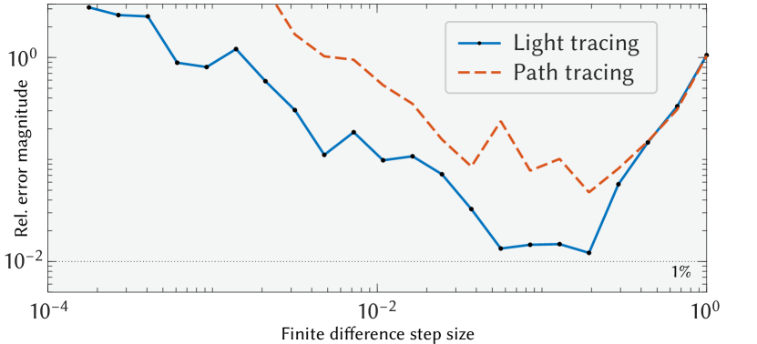
Figure S2. Finite difference errors of light tracing vs. path tracing: equal time comparison, where all evaluations start with a new, arbitrary random seed.

Further gradient comparison

In Fig. S2 we extend the comparison in §6.2 of our adjoint light tracing to a reference differentiable path tracing implementation that also uses our view-independent data structure to deliver the rendered radiance field and evaluate the same objective function. For a comparison that is indicative of optimization performance, we choose a new arbitrary random seed for each evaluation during finite difference approximation. In this way, the finite difference errors reveal that the path tracing approach produces less accurate gradients (due to sampling noise) in an equal time comparison to our method. Note that choosing new random seeds is more applicable in an optimization context, where we want sampling noise to average out over the course of the optimization procedure, rather than optimize for a specific noise pattern.

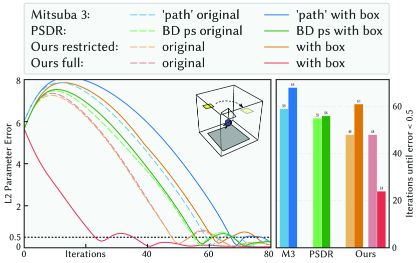
Figure S3. Adding a box around all objects in the test scene of Fig. 6.2, leads to different convergence behaviour. Using only camera-visible data reduces optimization performance when adding indirect illumination, whereas taking the full radiance field into account improves performance by ca. $50\%$ in terms of the number of iterations needed to reduce the parameter-space error below $0.5$ (dark red bar and line). We use the same optimization and render settings as in the original test.

Table 2. Summary of all methods and their performance in our comparisons. (: works, : converges quickly, $\boldsymbol{\mathbf{\thicksim}}$ : converges eventually, : available without observable effect, : image-based, : view-independent, $/$: camera-visible data only)

Method	$dO/d\boldsymbol{\mathbf{p}}$	Discont.	Space	Converges
M3: ’path’	AD
M3: ’ptracer’	AD
M3: ’prb-reparam’	Adjoint			$\boldsymbol{\mathbf{\thicksim}}$
PSDR: PT ps	AD
PSDR: LT ps	AD
PSDR: BD ps	AD
Our PT (full)	Adjoint
Our LT (full)	Adjoint
Our PT (restr.)	Adjoint		$/$
Our LT (restr.)	Adjoint		$/$
Our LT (naïve)	Direct

Extended baseline comparison

In our baseline test case (Fig. 6.2) we intentionally avoid most global influences caused by indirect illumination. As expected, our novel view-independent approach performs comparable to state-of-the-art image-based methods, regardless of whether we restrict our method to camera-visible surfaces, or evaluate the entire scene. In Fig. S3, we now extend the test scene by adding a box around all other objects, which increases the contribution of indirect illumination to the bunny and the background plane. Image-based methods, as well as our method when using restricted data for comparison, now converge slightly slower than in the original case (without the box). However, using our method and the full radiance data (including the box) as a target, improves the convergence rate by roughly $50\%$, demonstrating the advantage of a view-independent approach. When completing the entire optimization ($80$ iterations), our method is about $3\times$ faster than Mitsuba’s path tracer on this scene. Conversely, for image-based methods we would need to introduce additional cameras that cover the new surfaces of the box to achieve a similar effect. Table 2 gives an overview of all methods used and summarizes their features.

Gradient contribution visualization

Figure S4. Our gradient contribution visualization under indirect illumination, showing derivatives of the objective wrt. the $z$ coordinate (left-to-right in this view) of a spot light. Our method (a) visualizes contributions of adjoint states at the first ray-surface intersection of light paths reaching the target (b, inset) after some indirect bounces. Note that paths traversing points in the outer cone of the spot light (where the light’s intensity is attenuated) would increase in brightness if the light were to move to the right, while most other surfaces prefer the light moving left. Direct (non-adjoint) differentiation (c), or finite difference approximation (d) instead visualize indirect gradient contributions at the target surface itself. Image (b) shows the global illumination solution.

In this section, we show extended comparisons for our gradient contribution visualization introduced in §5. We first expand Fig. 7 with additional comparisons showing all three light position coordinates in Fig. S5. We again show results for finite differencing ($\Delta L/\Delta\boldsymbol{\mathbf{p}}$), direct (i.e. non-adjoint) differentiation ($dL/d\boldsymbol{\mathbf{p}})$, and our adjoint state ($\partial O/\partial\Phi_{r}$).

We then show an additional visualization example, Fig. S4 for an intermediate lighting configuration that occurs during the optimization shown in Fig. 10. At this point, the spot light has not navigated around the final corner in the labyrinth, so the target is still only illuminated by indirect light. In this situation, the difference between our adjoint approach, and a direct differentiation method (akin to forward-mode autodiff) is most clearly visible. Direct differentiation produces a similar result as a finite difference approximation, visualizing contributions to the objective function gradient at the target surface (after indirect light arrives there). Our approach, on the other hand, transports information about objective function derivatives backwards along light paths and visualizes the resulting gradient contribution at the first ray-surface intersection along these paths. In this way, we can observe how (indirect) light paths passing through parts of the surface near the light source contribute to the objective gradient at the target surface. Note that the objective gradient (which is integrated over all such contributions on surfaces) still pulls the light left towards the target.

Figure S5. Extended version of Fig. 7, our gradient visualization on the Stanford Dragon. The second to fourth rows show objective function gradient contributions for each position coordinate of the light source. Columns show our adjoint gradients (left), direct differentiation (centre), and finite difference approximation (right). Image subtitles indicate the calculation; BRDF derivatives are taken into account but not explicitly stated here for brevity.

References

- [1]
- ANSI/IES [2020] ANSI/IES. 2020. IES Standard File Format for Photometric Data, ANSI/IES LM-63-19. https://webstore.ansi.org/Standards/IESNA/ANSIIESLM6319
- Bangaru et al. [2020] Sai Praveen Bangaru, Tzu-Mao Li, and Frédo Durand. 2020. Unbiased warped-area sampling for differentiable rendering. ACM Transactions on Graphics 39, 6 (2020), 1–18. https://doi.org/10.1145/3414685.3417833
- Boyé et al. [2010] S. Boyé, G. Guennebaud, and C. Schlick. 2010. Least Squares Subdivision Surfaces. Computer Graphics Forum 29, 7 (sep 2010), 2021–2028. https://doi.org/10.1111/j.1467-8659.2010.01788.x
- Bradley [2019] Andrew M. Bradley. 2019. PDE-constrained optimization and the adjoint method. (2019). https://cs.stanford.edu/~ambrad/adjoint_tutorial.pdf
- DIAL GmbH [2022] DIAL GmbH. 2022. DIALux evo 10.1. https://www.dialux.com/en-GB/dialux
- Gautron et al. [2004] Pascal Gautron, Jaroslav Krivanek, Sumanta Pattanaik, and Kadi Bouatouch. 2004. A Novel Hemispherical Basis for Accurate and Efficient Rendering. Eurographics Workshop on Rendering (2004). https://doi.org/10.2312/EGWR/EGSR04/321-330
- Geilinger et al. [2020] Moritz Geilinger, David Hahn, Jonas Zehnder, Moritz Bächer, Bernhard Thomaszewski, and Stelian Coros. 2020. ADD: analytically differentiable dynamics for multi-body systems with frictional contact. ACM Transactions on Graphics 39, 6 (nov 2020), 1–15. https://doi.org/10.1145/3414685.3417766
- Gkaravelis [2016] Anastasios Gkaravelis. 2016. Inverse lighting design using a coverage optimization strategy. The Visual Computer 32, 6 (2016), 10.
- Gkioulekas et al. [2016] Ioannis Gkioulekas, Anat Levin, and Todd Zickler. 2016. An Evaluation of Computational Imaging Techniques for Heterogeneous Inverse Scattering. In Computer Vision – ECCV 2016. Springer International Publishing, 685–701. https://doi.org/10.1007/978-3-319-46487-9_42
- Gkioulekas et al. [2013] Ioannis Gkioulekas, Shuang Zhao, Kavita Bala, Todd Zickler, and Anat Levin. 2013. Inverse volume rendering with material dictionaries. ACM Transactions on Graphics 32, 6 (nov 2013), 1–13. https://doi.org/10.1145/2508363.2508377
- Goral et al. [1984] Cindy M. Goral, Kenneth E. Torrance, Donald P. Greenberg, and Bennett Battaile. 1984. Modeling the interaction of light between diffuse surfaces. ACM SIGGRAPH Computer Graphics 18, 3 (jul 1984), 213–222. https://doi.org/10.1145/964965.808601
- Green [2003] Robin Green. 2003. Spherical harmonic lighting: The gritty details. In Archives of the game developers conference, Vol. 56. 4. https://theory.cpe.ku.ac.th/~pramook/files/spherical-harmonic-lighting.pdf
- Greenberg et al. [1986] Donald P. Greenberg, Michael F. Cohen, and Kenneth E. Torrance. 1986. Radiosity: A method for computing global illumination. The Visual Computer 2, 5 (sep 1986), 291–297. https://doi.org/10.1007/bf02020429
- Hansen [2021] Nikolaus Hansen. 2021. c-cmaes. https://github.com/CMA-ES/c-cmaes
- Hansen et al. [2003] Nikolaus Hansen, Sibylle D. Müller, and Petros Koumoutsakos. 2003. Reducing the Time Complexity of the Derandomized Evolution Strategy with Covariance Matrix Adaptation (CMA-ES). Evolutionary Computation 11, 1 (mar 2003), 1–18. https://doi.org/10.1162/106365603321828970
- Hašan et al. [2009] Miloš Hašan, Jaroslav Křivánek, Bruce Walter, and Kavita Bala. 2009. Virtual spherical lights for many-light rendering of glossy scenes. ACM Transactions on Graphics 28, 5 (dec 2009), 1–6. https://doi.org/10.1145/1618452.1618489
- Jakob et al. [2022] Wenzel Jakob, Sébastien Speierer, Nicolas Roussel, Merlin Nimier-David, Delio Vicini, Tizian Zeltner, Baptiste Nicolet, Miguel Crespo, Vincent Leroy, and Ziyi Zhang. 2022. Mitsuba 3 renderer. https://mitsuba-renderer.org.
- Jensen [1996] Henrik Wann Jensen. 1996. Global Illumination using Photon Maps. In Eurographics. Springer Vienna, 21–30. https://doi.org/10.1007/978-3-7091-7484-5_3
- Jin and Lee [2019] Sam Jin and Sung-Hee Lee. 2019. Lighting Layout Optimization for 3D Indoor Scenes. Computer Graphics Forum 38, 7 (2019), 733–743. https://doi.org/10.1111/cgf.13875 _eprint: https://onlinelibrary.wiley.com/doi/pdf/10.1111/cgf.13875.
- Kajiya [1986] James T. Kajiya. 1986. The rendering equation. ACM SIGGRAPH Computer Graphics 20, 4 (aug 1986), 143–150. https://doi.org/10.1145/15886.15902
- Khungurn et al. [2015] Pramook Khungurn, Daniel Schroeder, Shuang Zhao, Kavita Bala, and Steve Marschner. 2015. Matching Real Fabrics with Micro-Appearance Models. ACM Transactions on Graphics 35, 1 (dec 2015), 1–26. https://doi.org/10.1145/2818648
- Kingma and Ba [2014] Diederik P. Kingma and Jimmy Ba. 2014. ADAM: A Method for Stochastic Optimization. (Dec. 2014). arXiv:1412.6980 [cs.LG]
- Krivanek et al. [2005] J. Krivanek, P. Gautron, S. Pattanaik, and K. Bouatouch. 2005. Radiance Caching for Efficient Global Illumination Computation. IEEE Transactions on Visualization and Computer Graphics 11, 5 (sep 2005), 550–561. https://doi.org/10.1109/tvcg.2005.83
- Larson and Bengzon [2013] Mats Larson and Fredrik Bengzon. 2013. The Finite Element Method: Theory, Implementation, and Applications. Springer-Verlag GmbH.
- Lehtinen et al. [2008] Jaakko Lehtinen, Matthias Zwicker, Emmanuel Turquin, Janne Kontkanen, Frédo Durand, François X. Sillion, and Timo Aila. 2008. A meshless hierarchical representation for light transport. ACM Transactions on Graphics 27, 3 (aug 2008), 1–9. https://doi.org/10.1145/1360612.1360636
- Li et al. [2018] Tzu-Mao Li, Miika Aittala, Frédo Durand, and Jaakko Lehtinen. 2018. Differentiable Monte Carlo ray tracing through edge sampling. ACM Transactions on Graphics 37, 6 (dec 2018), 1–11. https://doi.org/10.1145/3272127.3275109
- Lin et al. [2013] Wen-Chieh Lin, Tsung-Shian Huang, Tan-Chi Ho, Yueh-Tse Chen, and Jung-Hong Chuang. 2013. Interactive Lighting Design with Hierarchical Light Representation. Computer Graphics Forum 32, 4 (2013), 133–142. https://doi.org/10.1111/cgf.12159
- Liu et al. [2018] Hsueh-Ti Derek Liu, Michael Tao, and Alec Jacobson. 2018. Paparazzi: Surface Editing by way of Multi-View Image Processing. ACM Transactions on Graphics 37, 6 (dec 2018), 1–11. https://doi.org/10.1145/3272127.3275047
- Loubet et al. [2019] Guillaume Loubet, Nicolas Holzschuch, and Wenzel Jakob. 2019. Reparameterizing discontinuous integrands for differentiable rendering. ACM Transactions on Graphics 38, 6 (2019). https://doi.org/10.1145/3355089.3356510
- Luksch et al. [2019] Christan Luksch, Michael Wimmer, and Michael Schwärzler. 2019. Incrementally baked global illumination. In Proceedings of the ACM SIGGRAPH Symposium on Interactive 3D Graphics and Games. ACM. https://doi.org/10.1145/3306131.3317015
- Nimier-David et al. [2020] Merlin Nimier-David, Sébastien Speierer, Benoît Ruiz, and Wenzel Jakob. 2020. Radiative backpropagation. ACM Transactions on Graphics 39, 4 (jul 2020). https://doi.org/10.1145/3386569.3392406
- Nimier-David et al. [2019] Merlin Nimier-David, Delio Vicini, Tizian Zeltner, and Wenzel Jakob. 2019. Mitsuba 2: a retargetable forward and inverse renderer. ACM Transactions on Graphics 38, 6 (2019). https://doi.org/10.1145/3355089.3356498
- Nocedal [1980] Jorge Nocedal. 1980. Updating quasi-Newton matrices with limited storage. Math. Comp. 35, 151 (1980), 773–782. https://doi.org/10.1090/s0025-5718-1980-0572855-7
- Omidvar et al. [2015] Mahmoud Omidvar, Mickaël Ribardière, Samuel Carré, Daniel Méneveaux, and Kadi Bouatouch. 2015. A radiance cache method for highly glossy surfaces. The Visual Computer 32, 10 (oct 2015), 1239–1250. https://doi.org/10.1007/s00371-015-1159-y
- Pellacini et al. [2007] Fabio Pellacini, Frank Battaglia, R. Keith Morley, and Adam Finkelstein. 2007. Lighting with paint. ACM Transactions on Graphics 26, 2 (June 2007), 9. https://doi.org/10.1145/1243980.1243983
- Poulin et al. [1997] P. Poulin, K. Ratib, and M. Jacques. 1997. Sketching shadows and highlights to position lights. In Proceedings Computer Graphics International. IEEE Comput. Soc. Press, Hasselt and Diepenbeek, Belgium, 56–63. https://doi.org/10.1109/CGI.1997.601272
- Qiu [2021] Yixuan Qiu. 2021. LBFGS++. https://github.com/yixuan/LBFGSpp
- Relux Informatik AG [2022] Relux Informatik AG. 2022. ReluxDesktop. https://reluxnet.relux.com/en
- Schwarz and Wonka [2014] Michael Schwarz and Peter Wonka. 2014. Procedural Design of Exterior Lighting for Buildings with Complex Constraints. ACM Transactions on Graphics 33, 5 (sep 2014), 1–16. https://doi.org/10.1145/2629573
- Shesh and Chen [2007] Amit Shesh and Baoquan Chen. 2007. Crayon lighting: sketch-guided illumination of models. In Proceedings of the 5th international conference on Computer graphics and interactive techniques in Australia and Southeast Asia - GRAPHITE ’07. ACM Press, Perth, Australia, 95. https://doi.org/10.1145/1321261.1321278
- Sillion et al. [1991] Françis X. Sillion, James R. Arvo, Stephen H. Westin, and Donald P. Greenberg. 1991. A global illumination solution for general reflectance distributions. In Proceedings of the 18th annual conference on Computer graphics and interactive techniques - SIGGRAPH '91. ACM Press. https://doi.org/10.1145/122718.122739
- Sloan et al. [2002] Peter-Pike Sloan, Jan Kautz, and John Snyder. 2002. Precomputed radiance transfer for real-time rendering in dynamic, low-frequency lighting environments. ACM Transactions on Graphics 21, 3 (jul 2002), 527–536. https://doi.org/10.1145/566654.566612
- Sorger et al. [2016] Johannes Sorger, Thomas Ortner, Christian Luksch, Michael Schwarzler, Eduard Groller, and Harald Piringer. 2016. LiteVis: Integrated Visualization for Simulation-Based Decision Support in Lighting Design. IEEE Transactions on Visualization and Computer Graphics 22, 1 (Jan. 2016), 290–299. https://doi.org/10.1109/TVCG.2015.2468011
- Stam [2020] Jos Stam. 2020. Computing Light Transport Gradients using the Adjoint Method. (June 2020). arXiv:2006.15059 [cs.GR]
- Veach [1998] Eric Veach. 1998. Robust Monte Carlo Methods for Light Transport Simulation. Ph. D. Dissertation. Stanford, CA, USA. Advisor(s) Guibas, Leonidas J. https://dl.acm.org/doi/10.5555/927297 AAI9837162.
- Vicini et al. [2021] Delio Vicini, Sébastien Speierer, and Wenzel Jakob. 2021. Path replay backpropagation. ACM Transactions on Graphics 40, 4 (aug 2021), 1–14. https://doi.org/10.1145/3450626.3459804
- Walch et al. [2019] Andreas Walch, Michael Schwärzler, Christian Luksch, Elmar Eisemann, and Theresia Gschwandtner. 2019. LightGuider: Guiding Interactive Lighting Design using Suggestions, Provenance, and Quality Visualization. IEEE Transactions on Visualization and Computer Graphics (2019), 1–1. https://doi.org/10.1109/tvcg.2019.2934658
- Wieczorek and Meschede [2018] Mark A. Wieczorek and Matthias Meschede. 2018. SHTools: Tools for Working with Spherical Harmonics. Geochemistry, Geophysics, Geosystems 19, 8 (aug 2018), 2574–2592. https://doi.org/10.1029/2018gc007529
- Yan et al. [2022] Kai Yan, Christoph Lassner, Brian Budge, Zhao Dong, and Shuang Zhao. 2022. Efficient estimation of boundary integrals for path-space differentiable rendering. ACM Transactions on Graphics 41, 4 (jul 2022), 1–13. https://doi.org/10.1145/3528223.3530080
- Yu et al. [2021] Alex Yu, Sara Fridovich-Keil, Matthew Tancik, Qinhong Chen, Benjamin Recht, and Angjoo Kanazawa. 2021. Plenoxels: Radiance Fields without Neural Networks. (Dec. 2021). arXiv:2112.05131 [cs.CV]
- Zeltner et al. [2021] Tizian Zeltner, Sébastien Speierer, Iliyan Georgiev, and Wenzel Jakob. 2021. Monte Carlo estimators for differential light transport. ACM Transactions on Graphics 40, 4 (aug 2021), 1–16. https://doi.org/10.1145/3450626.3459807
- Zhang et al. [2020] Cheng Zhang, Bailey Miller, Kai Yan, Ioannis Gkioulekas, and Shuang Zhao. 2020. Path-space differentiable rendering. ACM Transactions on Graphics 39, 4 (2020). https://doi.org/10.1145/3386569.3392383
- Zhang et al. [2019] Cheng Zhang, Lifan Wu, Changxi Zheng, Ioannis Gkioulekas, Ravi Ramamoorthi, and Shuang Zhao. 2019. A differential theory of radiative transfer. ACM Transactions on Graphics 38, 6 (2019). https://doi.org/10.1145/3355089.3356522