Federated Wasserstein Distance

Abstract

We introduce a principled way of computing the Wasserstein distance between two distributions in a federated manner. Namely, we show how to estimate the Wasserstein distance between two samples stored and kept on different devices/clients whilst a central entity/server orchestrates the computations (again, without having access to the samples). To achieve this feat, we take advantage of the geometric properties of the Wasserstein distance – in particular, the triangle inequality – and that of the associated geodesics: our algorithm, FedWaD (for Federated Wasserstein Distance), iteratively approximates the Wasserstein distance by manipulating and exchanging distributions from the space of geodesics in lieu of the input samples. In addition to establishing the convergence properties of FedWaD, we provide empirical results on federated coresets and federate optimal transport dataset distance, that we respectively exploit for building a novel federated model and for boosting performance of popular federated learning algorithms.

1 Introduction

Context.

Federated Learning (FL) is a form of distributed machine learning (ML) dedicated to train a global model from data stored on local devices/clients, while ensuring these clients never share their data (Kairouz et al., 2021; Wang et al., 2021). FL provides elegant and convenient solutions to concerns in data privacy, computational and storage costs of centralized training, and makes it possible to take advantage of large amounts of data stored on local devices. A typical FL approach to learn a parameterized global model is to alternate between the two following steps: i) update local versions of the global model using local data, and ii) send and aggregate the parameters of the local models on a central server (McMahan et al., 2017) to update the global model.

Problem.

In some practical situations, the goal is not to learn a prediction model, but rather to compute a certain quantity from the data stored on the clients. For instance, one’s goal may be to compute, in a federated way, some prototypes of client’s data, that can be leveraged for federated clustering or for classification models (Gribonval et al., 2021; Phillips, 2016; Munteanu et al., 2018; Agarwal et al., 2005). In another learning scenarios where data are scarce, one may want to look for similarity between datasets in order to evaluate dataset heterogeneity over clients and leverage on this information to improve the performance of federated learning algorithms. In this work, we address the problem of computing, in a federated way, the Wasserstein distance between two distributions $\mu$ and $\nu$ when samples from each distribution are stored on local devices. A solution to this problem will be useful in the aforementioned situations, where the Wasserstein distance is used as a similarity measure between two datasets and is the key tool for computing some coresets of the data distribution or cluster prototypes. We provide a solution to this problem which hinges on the geometry of the Wasserstein distance and more specifically, its geodesics. We leverage the property that for any element $\xi^{\star}$ of the geodesic between two distributions $\mu$ and $\nu$, the following equality holds, $\mathcal{W}_{p}(\mu,\nu)=\mathcal{W}_{p}(\mu,\xi^{\star})+\mathcal{W}_{p}(\xi^{\star},\nu)$, where $\mathcal{W}_{p}$ denotes the $p$-Wasserstein distance. This property is especially useful to compute $\mathcal{W}_{p}(\mu,\nu)$ in a federated manner, leading to a novel theoretically-justified procedure coined FedWaD, for Federated Wasserstein Distance.

Contribution: FedWaD.

The principle of FedWaD is to iteratively approximate $\xi^{\star}$ – which, in terms of traditional FL, can be interpreted as the global model. At iteration $k$, our procedure consists in i) computing, on the clients, distributions $\xi_{\mu}^{k}$ and $\xi_{\nu}^{k}$ from the geodesics between the current approximation of $\xi^{\star}$ and the two secluded distributions $\mu$ and $\nu$ – $\xi_{\mu}^{k}$ and $\xi_{\nu}^{k}$ playing the role of the local versions of the global model, and ii) aggregating them on the global model to update $\xi^{\star}$.

Organization of the paper.

Section 2 formalizes the problem we address, and provides the necessary technical background to devise our algorithm FedWaD. Section 3 is devoted to the depiction of FedWaD, pathways to speed-up its executions, and a theoretical justification that FedWaD is guaranteed to converge to the desired quantity. In Section 4, we conduct an empirical analysis of FedWaD on different use-cases (Wasserstein coresets and Optimal Transport Dataset distance) which rely on the computation of the Wasserstein distance. We unveil how these problems can be solved in our FL setting and demonstrates the remarkable versatility of our approach. In particular, we expose the impact of federated coresets. By learning a single global model on the server based on the coreset, our method can outperform personalized FL models. In addition, our ability to compute inter-device dataset distances significantly helps amplify performances of popular federated learning algorithms, such as FedAvg, FedRep, and FedPer. We achieve this by clustering clients and harnessing the power of reduced dataset heterogeneity.

2 Related Works and Background

2.1 Wasserstein Distance and Geodesics

Throughout, we denote by $\mathscr{P}(X)$ the set of probability measures in $X$. Let $p\geq 1$ and define $\mathscr{P}_{p}(X)$ the subset of measures in $\mathscr{P}(X)$ with finite $p$-moment, i.e., $\mathscr{P}_{p}(X)\doteq\big{\{}\eta\in\mathscr{P}(X):M_{p}(\eta)<\infty\big{\}}$, where $M_{p}(\eta)\doteq\int_{X}{d^{p}_{X}(x,0)}d\eta(x)$ and $d_{X}$ is a metric on $X$ often referred to as the ground cost. For $\mu\in\mathscr{P}_{p}(X)$ and $\nu\in\mathscr{P}_{p}(Y)$, $\Pi(\mu,\nu)\subset\mathscr{P}(X\times Y)$ is the collection of probability measures or couplings on $X\times Y$ defined as

$$\Pi(\mu,\nu)\doteq\big{\{} \pi\in\mathscr{P}(X\times Y):\forall A\subset X,B\subset Y,\pi(A\times Y)=\mu(A)\text{ and }\pi(X\times B)=\nu(B)\big{\}}.$$

The $p$-Wasserstein distance $\mathcal{W}_{p}(\mu,\nu)$ between the measures $\mu$ and $\nu$ —assumed to be defined over the same ground space, i.e. $X=Y$— is defined as

$$\mathcal{W}_{p}(\mu,\nu)\doteq\left(\inf_{\pi\in\Pi(\mu,\nu)}\int_{X\times X}d^{p}_{X}(x,x^{\prime})d\pi(x,x^{\prime})\right)^{1/p}.$$ (1)

It is proven that the infimum in (1) is attained (Peyré et al., 2019) and any probability $\pi$ which realizes the minimum is an optimal transport plan. In the discrete case, we denote the two marginal measures as $\mu=\sum_{i=1}^{n}a_{i}\delta_{x_{i}}$ and $\nu=\sum_{i=1}^{m}b_{i}\delta_{x_{i}^{\prime}}$, with $a_{i},b_{i}\geq 0$ and $\sum_{i=1}^{n}a_{i}=\sum_{i=1}^{m}b_{i}=1$. The Kantorovitch relaxation of (1) seeks for a transportation coupling $\mathbf{P}$ that solves the problem

$$\mathcal{W}_{p}(\mu,\nu)\doteq\left(\min_{\mathbf{P}\in\Pi(\mathbf{a},\mathbf{b})}\langle\mathbf{C},\mathbf{P}\rangle\right)^{1/p}$$ (2)

where $\mathbf{C}\doteq(d_{X}^{p}(x_{i},x_{j}^{\prime}))\in\mathbb{R}^{n\times m}$ is the matrix of all pairwise costs, and $\Pi(\mathbf{a},\mathbf{b})\doteq\{\mathbf{P}\in\mathbb{R}_{+}^{n\times m}|\mathbf{P}\mathbf{1}=\mathbf{a},\mathbf{P}^{\top}\mathbf{1}=\mathbf{b}\}$ is the transportation polytope (i.e. the set of all transportation plans) between the distributions $\mathbf{a}$ and $\mathbf{b}$.

Property 1 (Peyré et al. (2019)).

For any $p\geq 1$, $\mathcal{W}_{p}$ is a metric on $\mathscr{P}_{p}(X)$. As such it satisfies the triangle inequality:

$$\forall\mu,\nu,\xi\in\mathscr{P}_{p}(X),\quad\mathcal{W}_{p}(\mu,\nu)\leq\mathcal{W}_{p}(\mu,\xi)+\mathcal{W}_{p}(\xi,\nu)$$ (3)

It might be convenient to consider geodesics as structuring tools of metric spaces.

Definition 1 (Geodesics, (Ambrosio et al., 2005)).

Let ($\mathcal{X},\text{d}$) be a metric space. A constant speed geodesic $x:[0,1]\rightarrow\mathcal{X}$ between $x_{0},x_{1}$ $\in\mathcal{X}$ is a continuous curve such that $\forall s,t\in[0,1]$, $\text{d}(x(s),x(t))=|s-t|\cdot\text{d}(x_{0},x_{1}).$

Property 2 (Interpolating point, (Ambrosio et al., 2005)).

Any point $x_{t}$ from a constant speed geodesic $(x(t))_{t\in[0,1]}$ is an interpolating point and verifies, $d(x_{0},x_{1})=d(x_{0},x_{t})+d(x_{t},x_{1}),$ i.e. the triangle inequality becomes an equality.

These definitions and properties carry over to the case of the Wasserstein distance:

Definition 2 (Wasserstein Geodesics, Interpolating measure, (Ambrosio et al., 2005; Kolouri et al., 2017)).

Let $\mu_{0}$, $\mu_{1}$ $\in\mathscr{P}_{p}(X)$ with $X\subseteq\mathbb{R}^{d}$ compact, convex and equipped with $\mathcal{W}_{p}$. Let $\gamma\in\Pi(\mu_{0},\mu_{1})$ be an optimal transport plan. For $t\in[0,1],$ let $\mu_{t}\doteq(\pi_{t})_{\#}\gamma$ where $\pi_{t}(x,y)\doteq(1-t)x+ty$, i.e. $\mu_{t}$ is the push-forward measure of $\gamma$ under the map $\pi_{t}$. Then, the curve $\bar{\mu}\doteq(\mu_{t})_{t\in[0,1]}$ is a constant speed geodesic between $\mu_{0}$ and $\mu_{1};$ we call it a Wasserstein geodesics between $\mu_{0}$ and $\mu_{1}.$

Any point $\mu_{t}$ of the geodesics is an interpolating measure between $\mu_{0}$ and $\mu_{1}$ and, as expected:

$$\mathcal{W}_{p}(\mu_{0},\mu_{1})=\mathcal{W}_{p}(\mu_{0},\mu_{t})+\mathcal{W}_{p}(\mu_{t},\mu_{1}).$$ (4)

In the discrete case, and for a fixed $t$, one can obtain such interpolating measure $\mu_{t}$ given the optimal transport map $\mathbf{P}^{\star}$ solution of Equation 2 as follows (Peyré et al., 2019, Remark 7.1):

$$\mu_{t}=\sum_{i,j}^{n,m}\mathbf{P}_{i,j}^{\star}\delta_{(1-t)x_{i}+tx_{j}^{\prime}}$$ (5)

where $\mathbf{P}_{i,j}^{\star}$ is the $(i,j)$-th entry of $\mathbf{P}^{\star}$; as an interpolating measure, $\mu_{t}$ obviously complies with (4).

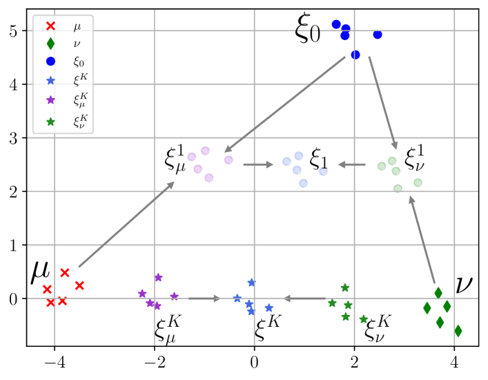
• At first iteration the current estimation $\xi_{0}$ of $\xi^{\star}$ is sent to each client in order to compute two interpolating measures $\xi_{\mu}^{1}$ and $\xi_{\nu}^{1}$, which are sent back to the server.

• Server then computes an interpolating measure between $\xi_{\mu}^{1}$ and $\xi_{\nu}^{1}$ to obtain the next iterate of the geodesic element $\xi^{1}$

• The process is repeated until convergence to obtain $\xi^{K}$ and we define $\mathcal{W}_{p}(\mu,\nu)=\mathcal{W}_{p}(\mu,\xi^{K})+\mathcal{W}_{p}(\nu,\xi^{K})$.

Figure 1: The Wasserstein distance between $\mu$ and $\nu$ which are on their respective clients can be computed as $\mathcal{W}_{p}(\mu,\nu)=\mathcal{W}_{p}(\mu,\xi^{\star})+\mathcal{W}_{p}(\nu,\xi^{\star})$ where $\xi^{\star}$ is an element on the geodesic between $\mu$ and $\nu$. FedWaD seeks at estimating $\xi^{\star}$ with $\xi^{K}$ using an iterative algorithm and plugs in this estimation to obtain $\mathcal{W}_{p}(\mu,\nu)$. Iterates of $\xi_{i}$ are computed on the server and sent to clients in order to compute measures $\xi_{\mu}^{i}$ and $\xi_{\nu}^{i}$ that are on geodesics of $\mu$ and $\xi_{i}$ and $\nu$ and $\xi_{i}$ respectively.

2.2 Problem Statement

Our goal is to compute the Wasserstein distance between two data distributions $\mu$ and $\nu$ on a global server with the constraint that $\mu$ and $\nu$ are distributed on two different clients which do not share any data samples to the server. From a mathematical point of view, our objective is to estimate an element $\xi^{\star}$ on the geodesic of $\mu$ and $\nu$ without having access to them by leveraging two other elements $\xi_{\mu}$ and $\xi_{\nu}$ on the geodesics of $\mu$ and $\xi^{\star}$ and $\nu$ and $\xi^{\star}$ respectively.

2.3 Related Works

Our work touches the specific question of learning/approximating a distance between distributions whose samples are secluded on isolated clients. As far as we are aware of, this is a problem that has never been investigated before and there are only few works that we see closely connected to ours. Some problems have addressed the objective of retrieving nearest neighbours of one vector in a federated manner. For instance, Liu et al. (2021) consider to exchange encrypted versions of the dataset on client to the central server and Schoppmann et al. (2018) consider the exchange of differentially private statistics about the client dataset. Zhang et al. (2023) propose a federated approximate $k$-nearest approach based on a specific spatial data federation. Compared to these works that compute distances in a federated manner, we address the case of distances on distributions without any specific encryption of the data and we exploit the properties of the Wasserstein distances and its geodesics, which have been overlooked in the mentioned works. If these properties have been relied upon as a key tool in some computer vision applications (Bauer et al., 2015; Maas et al., 2017) and trajectory inference (Huguet et al., 2022), they have not been employed as a privacy-preserving tool.

3 Computing the Federated Wasserstein distance

In this section, we develop a methodology to compute, on a global server, the Wasserstein distance between two distributions $\mu$ and $\nu$, stored on two different clients which do not share this information to the server. Our approach leverages the topology induced by the Wasserstein distance in the space of probability measures, and more precisely, the geodesics.

Outline of our methodology. A key property is that $\mathcal{W}_{p}$ is a metric, thus satisfies the triangle inequality: for any $\mu,\nu,\xi\in\mathscr{P}_{p}(X)$,

$$\mathcal{W}_{p}(\mu,\nu)\leq\mathcal{W}_{p}(\mu,\xi)+\mathcal{W}_{p}(\xi,\nu)\,,$$ (6)

with equality if and only if $\xi=\xi^{\star}$, where $\xi^{\star}$ is an interpolating measure. Consequently, one can compute $\mathcal{W}_{p}(\mu,\nu)$ by computing $\mathcal{W}_{p}(\mu,\xi^{\star})$ and $\mathcal{W}_{p}(\xi^{\star},\nu)$ and adding these two terms. This result is useful in the federated setting and inspires our methodology, as described hereafter. The global server computes $\xi^{\star}$ and communicate $\xi^{\star}$ to the two clients. The clients respectively compute $\mathcal{W}_{p}(\mu,\xi^{\star})$ and $\mathcal{W}_{p}(\xi^{\star},\nu)$, then send these to the global server. Finally, the global server adds the two received terms to return $\mathcal{W}_{p}(\mu,\nu)$.

The main bottleneck of this procedure is that the global server needs to compute $\xi^{\star}$ (which by definition, depends on $\mu,\nu$) while not having access to $\mu,\nu$ (which are stored on two clients). We then propose a simple workaround to overcome this challenge, based on an additional application of the triangle inequality: for any $\xi\in\mathscr{P}_{p}(X)$,

$$\mathcal{W}_{p}(\mu,\nu)\leq\mathcal{W}_{p}(\mu,\xi)+\mathcal{W}_{p}(\xi,\nu)=\mathcal{W}_{p}(\mu,\xi_{\mu})+\mathcal{W}_{p}(\xi_{\mu},\xi)+\mathcal{W}_{p}(\xi,\xi_{\nu})+\mathcal{W}_{p}(\xi_{\nu},\nu)\,,$$ (7)

where $\xi_{\mu}$ and $\xi_{\nu}$ are interpolating measures respectively between $\mu$ and $\xi$ and $\xi$ and $\nu$. Hence, computing $\xi^{\star}$ can be done through intermediate measures $\xi_{\mu}$ and $\xi_{\nu}$, to ensure that $\mu,\nu$ stay on their respective clients. To this end, we develop an optimization procedure which essentially consists in iteratively estimating an interpolating measure $\xi^{(k)}$ between $\mu$ and $\nu$ on the server, by using $\xi_{\mu}^{(k)}$ and $\xi_{\nu}^{(k)}$ which were computed and communicated by the clients. More precisely, the objective is to minimize (7) over $\xi$ as follows: at iteration $k$, the clients receive current iterate $\xi^{(k-1)}$ and compute $\xi_{\mu}^{(k)}$ and $\xi_{\nu}^{(k)}$ (as interpolating measures between $\mu$ and $\xi^{(k-1)}$, and between $\xi^{(k-1)}$ and $\nu$ respectively). By the triangle inequality,

$$\mathcal{W}_{p}(\mu,\nu)\leq\mathcal{W}_{p}(\mu,\xi_{\mu}^{(k)})+\mathcal{W}_{p}(\xi_{\mu}^{(k)},\xi^{(k-1)})+\mathcal{W}_{p}(\xi^{(k-1)},\xi_{\nu}^{(k)})+\mathcal{W}_{p}(\xi_{\nu}^{(k)},\nu)\,,$$ (8)

therefore, the clients then send $\xi_{\mu}^{(k)}$ and $\xi_{\nu}^{(k)}$ to the server, which in turn, computes the next iterate $\xi^{(k)}$ by minimizing the left-hand side term of (8), i.e.,

$$\xi^{(k)}\in\mathop{\mathrm{arg\,min}}_{\xi}\mathcal{W}_{p}(\xi_{\mu}^{(k)},\xi)+\mathcal{W}_{p}(\xi,\xi_{\nu}^{(k)})\,.$$ (9)

Algorithm 1 FedWaD

0:  $\mu$ and $\nu$, initialisation of $\xi^{(0)}$, function InterpMeas that computes an interpolating measure between two measures using Equation 5 or Equation 10 for any $0<t<1$.

1:  for $k=1$ to $K$ do

2:     // Send $\xi^{(k-1)}$ to clients

3:     // Compute on clients with optional return of the distances

4:     $\xi_{\mu}^{(k)},[d_{\mu,\xi^{(k)}}]\leftarrow$ InterpMeas$(\mu,\xi^{(k-1)})$

5:     $\xi_{\nu}^{(k)},[d_{\xi^{(k),\nu}}]\leftarrow$ InterpMeas$(\nu,\xi^{(k-1)})$

6:     // Send $\xi_{\mu}^{(k)}$ and $\xi_{\nu}^{(k)}$ to server

7:     $\xi^{(k)}\leftarrow$ InterpMeas$(\xi_{\mu}^{(k)},\xi_{\nu}^{(k)})$

8:  end for

9:  // Send $d_{\mu,\xi^{(k)}}+d_{\xi^{(k),\nu}}$ to server

10:  $d_{\mu,\nu}=d_{\mu,\xi^{(K)}}+d_{\xi^{(K)},\nu}$

10:  return $d_{\mu,\nu}$ on server

Our methodology is illustrated in Figure 1 and summarized in Algorithm 1. Besides computing the Wasserstein distance in a federated manner, we point out several methods can easily be incorporated in our algorithm to further reduce the risk of privacy leak. Since the triangle inequality reaches equality on a particular geodesic, $\xi^{(k)}$, $\xi_{\mu}^{(k)}$ or $\xi_{\nu}^{(k)}$ are not unique, thus clients can compute these interpolating measures based on a random value of $t$. Besides, since communicating the distance may reveal information about the data, they can be shared with the server only for the last iteration. More effectively, one can incorporate an (adapted) differentially private version of the Wasserstein distance (Lê Tien et al., 2019). Regarding communication cost, at each iteration, the communication cost involves the transfer between the server and the clients of four interpolating measures: $\xi^{(k-1)}$ (twice), $\xi_{\mu}^{(k)}$, $\xi_{\nu}^{(k)}$. Hence, if the support size of $\xi^{(k-1)}$ is $S$, the communication cost is in $\mathcal{O}(4SKd)$, with $d$ the data dimension and $K$ the number of iterations.

Reducing the computational complexity.

In terms of computational complexity, we need to compute three OT plans per iteration which single cost, based on the network simplex is $O((n+m)nmlog(n+m))$. More importantly, consider that $\mu$ and $\nu$ are discrete measures, then, any interpolating measure between $\mu$ and $\nu$ is supported on at most on $n+m+1$ points. Hence, even if the size of the support of $\xi^{(0)}$ is small, but $n$ is large, the support of the next interpolating measures may get larger and larger, and this can yield an important computational overhead when computing $\mathcal{W}_{p}(\mu,\xi^{(k)})$ and $\mathcal{W}_{p}(\xi^{(k)},\nu)$.

To reduce this complexity, we resort to approximations of the interpolating measures which goal is to fix the support size of the interpolating measures to a small number $S$. The solution we consider is to approximate the McCann’s interpolation equation which formalizes geodesics $\xi_{t}$ given an optimal transport map between two distributions,say, $\xi$ and $\xi^{\prime}$, based on the equation $\xi_{t}=((1-t)Id+tT)_{\#}\xi$ Peyré et al. (2019). Using barycentric mapping approximation of the map $T$ (Courty et al., 2018), we propose to approximate the interpolating measures $\xi_{t}$ as

$$\xi_{t}=\frac{1}{n}\sum_{i=1}^{n}\delta_{(1-t)x_{i}+tn(\mathbf{P}^{\star}\mathbf{X}^{\prime})_{i}}$$ (10)

where $\mathbf{P}^{\star}$ is the optimal transportation plan between $\xi$ and $\xi^{\prime}$, $x_{i}$ and $x_{j}^{\prime}$ are the samples from these distributions and $\mathbf{X}^{\prime}$ is the matrix of samples from $\xi^{\prime}$. Note that by choosing the appropriate formulation of the equation, the support size of this interpolating measure can be chosen as the one of $\xi$ or $\xi^{\prime}$. In practice, we always opt for the choice that leads to the smallest support of the interpolating measure. Hence, if the support size of $\xi^{(0)}$ is $S$, we have the guarantee that the support of $\xi^{(k)}$ is $S$ for all $k$. Then, for computing $\mathcal{W}_{p}(\mu,\xi^{(k)})$ using approximated interpolating measures, it costs $O(3*(Sn^{2}+S^{2}n)log(n+S))$ at each iteration and if $S$ and the number of iterations $K$ are small enough, the approach we propose is even competitive compared to exact OT. Our experiments reported later that for larger number of samples ($\geq 5000$), our approach is as fast as exact optimal transport and less prone to numerical errors.

Theoretical guarantees.

We discuss in this section some theoretical properties of the components of FedWaD. At first, we show that the approximated interpolating measure is tight in the sense that there exists some situations where the resulting approximation is exact.

Theorem 1.

Consider two discrete distributions $\mu$ and $\nu$ with the same number of samples $n$ and uniform weights, then for any $t$, the approximated interpolating measure, between $\mu$ and $\nu$ given by Equation 10 is equal to the exact one Equation 5.

Proof is given in Appendix A. In practice, this property does not have much impact, but it ensures us about the soundness of the approach. In the next theorem, we prove that Algorithm 1 is theoretically justified, in the sense that its output converges to $\mathcal{W}_{p}(\mu,\nu)$.

Theorem 2.

Let $\mu$ and $\nu$ be two measures in $\mathscr{P}_{p}(X)$, $\xi_{\mu}^{(k)}$, $\xi_{\nu}^{(k)}$ and $\xi^{(k)}$ be the interpolating measures computed at iteration $k$ as defined in Algorithm 1. Denote as

$$A^{(k)}=\mathcal{W}_{p}(\mu,\xi_{\mu}^{(k)})+\mathcal{W}_{p}(\xi_{\mu}^{(k)},\xi^{(k)})+\mathcal{W}_{p}(\xi^{(k)},\xi_{\nu}^{(k)})+\mathcal{W}_{p}(\xi_{\nu}^{(k)},\nu)$$

Then the sequence $(A^{(k)})_{k}$ is non-increasing and converges to $\mathcal{W}_{p}(\mu,\nu)$.

We provide hereafter a sketch of the proof, and refer to Appendix B for full details. First, we show that the sequence $(A^{(k)})_{k}$ is non-increasing, as we iteratively update $\xi_{\mu}^{(k+1)}$, $\xi_{\nu}^{(k+1)}$ and $\xi^{(k+1)}$ based on geodesics (a minimizer of the triangle inequality). Then, we show that the sequence $(A^{(k)})_{k}$ is bounded below by $\mathcal{W}_{p}(\mu,\nu)$. We conclude the proof by proving that the sequence $(A^{(k)})_{k}$ converges to $\mathcal{W}_{p}(\mu,\nu)$.

In the next theorem, we show that when $\mu$ and $\nu$ are Gaussians then we can recover some nicer properties of our algorithm and provide a convergence rate (proof in Appendix C).

Theorem 3.

Assume that $\mu$, $\nu$ and $\xi^{(0)}$ are three Gaussian distributions with the same covariance matrix $\Sigma$ ie $\mu\sim\mathcal{N}(\mathbf{m}_{\mu},\Sigma)$, $\nu\sim\mathcal{N}(\mathbf{m}_{\nu},\Sigma)$ and $\xi^{(0)}\sim\mathcal{N}(\mathbf{m}_{\xi^{(0)}},\Sigma)$. Further assume that we are not in the trivial case where $\mathbf{m}_{\mu}$, $\mathbf{m}_{\nu}$, and $\mathbf{m}_{\xi^{(0)}}$ are aligned. Applying our Algorithm 1 with $t=0.5$ and the squared Euclidean cost, we have the following properties:

1. all interpolating measures $\xi_{\mu}^{(k)}$,$\xi_{\nu}^{(k)}$, $\xi^{(k)}$ are Gaussian distributions with the same covariance matrix $\Sigma$,

2. for any $k\geq 1$, $\mathcal{W}_{2}(\mu,\nu)=\|\mathbf{m}_{\mu}-\mathbf{m}_{\nu}\|_{2}=2\|\mathbf{m}_{\xi_{\mu}^{(k)}}-\mathbf{m}_{\xi_{\nu}^{(k)}}\|_{2}=2\mathcal{W}_{2}(\xi_{\mu}^{(k)},\xi_{\nu}^{(k)})$

3. $\mathcal{W}_{2}(\xi^{(k)},\xi^{\star})=\frac{1}{2}\mathcal{W}_{2}(\xi^{(k-1)},\xi^{\star})$

4. $\mathcal{W}_{2}(\mu,\xi^{(k)})+\mathcal{W}_{2}(\xi^{(k)},\nu)-\mathcal{W}_{2}(\mu,\nu)\leq\frac{1}{2^{k-1}}\mathcal{W}_{2}(\xi^{(0)},\xi^{(\star)})$

Interestingly, this theorem also says that in this specific case, only one iteration is needed to recover $\mathcal{W}_{2}(\mu,\nu)$

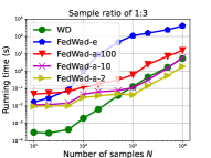
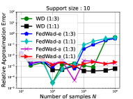
Figure 2: Analysis of the different Wasserstein distance computation methods (most-left panels) for varying support size of the approximated FedWaD and (most-right panels) for varying sample ratio in the two distributions and fixed support size. For each couple of panels, for increasing number of samples, we report the running time and the relative error of the Wasserstein distance (WD), our exact FedWaD (FedWad-e) and our approximate FedWaD (FedWad-a) with a support size of $2$, $10$ and $100$. For the most-right panels, we have set the support size of the interpolating measure to $10$. For a sample ratio (1:3), the first distribution has a number of samples $N$ and the second ones $N/3$.

4 Experiments

This section presents numerical applications, where FedWaD can successfully be used and show how it can boost performances of federated learning algorithms. Full details are provided in Appendix D.

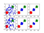
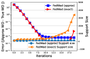
Figure 3: (left) Evolution of the interpolating measure $\xi^{(k)}$ - in blue - (right) the estimated Wasserstein distance between two Gaussian distributions $\mu$ and $\nu$.

Toy analysis.

We illustrate the evolution of interpolating measures using FedWaD  for calculating the Wasserstein distance between two Gaussian distributions. We sample 200 points from two 2D Gaussian distributions with different means and the same covariance matrix. We compute the interpolating measure at $t=0.5$ using both the analytical formula (5) and the approximation (10). Figure 3 (left panel) shows how the interpolating measure evolves across iterations. We also observe, in Figure 3 (right panel), that the error on the true Wasserstein distance for the approximated interpolating measure reaches $10^{-3}$, while for the exact interpolating measure, it drops to a minimum of $10^{-4}$ before increasing. This discrepancy occurs as the support size of the interpolating measure expands across iterations leading to numerical errors when computing the optimal transport plan between $\xi^{(k)}$ and $\xi_{\mu}^{(k)}$ or $\xi_{\nu}^{(k)}$. Hence, using the approximation Equation 10 is a more robust alternative to exact computation Equation 5.

We also examine computational complexity and approximation errors for both methods as we increase sample sizes in the distributions, as displayed in Figure 2. Key findings include: The approximated interpolating measure significantly improves computational efficiency, being at least 10 times faster with sample size exceeding 100, especially with smaller support sizes. It also achieves a similar relative approximation error as FedWaD using the exact interpolating measure and true non-federated Wasserstein distance. Importantly, it demonstrates greater robustness with larger sample sizes compared to true Wasserstein distance for such a small dimensional problem.

Wasserstein coreset and application to federated learning.

In many ML applications,

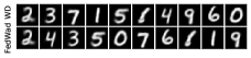
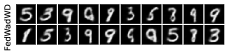
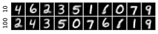
Figure 4: Examples of the $10$ coreset we obtained, with for each panel (top-row) the exact Wasserstein and (bottow-row) FedWaD for the MNIST dataset. Different panels correspond to different number of classes $K$ on each client: (top) $K=8$, (middle) $K=2$, (bottom) support of the interpolating measure varying from $10$ to $100$.

summarizing data into fewer representative samples is routinely done to deal with large datasets. The notion of coreset has been relevant to extract such samples and admit several formulations (Phillips, 2016; Munteanu et al., 2018). In this experiment, we show that Wasserstein coresets (Claici et al., 2018) can be computed in a federated way via FedWaD. Formally, given a dataset described by the distribution $\mu$, the Wasserstein coreset aims at finding the empirical distribution that minimizes $\min_{x_{1}^{\prime},\cdots,x_{K}^{\prime}}\mathcal{W}_{p}\left(\frac{1}{K}\sum_{i=1}^{K}\delta_{x_{i}^{\prime}},\mu\right)\,.$ We solve this problem in the following federated setting: we assume that either the samples drawn from $\mu$ are stored on an unique client or distributed across different clients, and the objective is to learn the coreset samples $\{x_{i}^{\prime}\}$ on the server. In our setting, we can compute the federated Wasserstein distances between the current coreset and some subsamples of all active client datasets, then update the coreset given the aggregated gradients of these distances with respect to the coreset support. We sampled $20000$ examples randomly from the MNIST dataset, and dispatched them at random on $100$ clients. We compare the results we obtained with FedWaD with those obtained with exact non-federated Wasserstein distance The results are shown in Figure 4. We can note that when classes are almost equally spread across clients (with $K=8$ different classes per client), FedWaD is able to capture the $10$ modes of the dataset. However, as the diversity in classes between clients increases, FedWaD has more difficulty to capture all the modes of the dataset. Nonetheless, we also observe that the exact Wasserstein distance is not able to recover those modes either. We can thus conjecture that this failure is likely due to the coreset approach itself, rather than to the approximated distance returned by FedWaD. We also note that the support size of the interpolating measure has less impact on the coreset. We believe this is a very interesting result, as it shows that FedWaD can provide useful gradient to the problem even with a poorer estimation of the distance.

Federated coreset classification model

Those federated coresets can also be used for classification tasks. As such, we have learned coresets for each client, and used all the coresets from all clients as the examples for a one-nearest neighbor global classifier shared to all clients. Note that since a coreset computation is an unsupervised task, we have assigned to each element of a coreset the label of the closest element in the client dataset. For this task, we have used the MNIST dataset which has been autoencoded in order to reduce its dimensionality. Half of the training samples have been used for learning the autoencoder and the other half for the classification task. Those samples and the test samples of dataset have been distributed across clients while ensuring that each client has samples from only $2$ classes. We have then computed the accuracy of this federated classifier for varying number of clients and number of coresets and compared its performance to the ones of FedRep (Collins et al., 2021) and FedPer (Arivazhagan et al., 2019). Results are reported in Figure 5. We can see that our simple approach is highly competitive with these personalized FL approaches, and even outperforms them when the number of users becomes large.

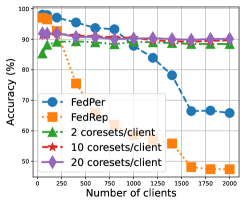
Figure 5: Nearest neighbor classifier based on the coresets learnt from each client for varying number of clients and number of coresets per clients We have compared to the performance of two personalized FL algorithms.

Geometric dataset distances via federated Wasserstein distance.

Our goal is to improve on the seminal algorithm of Alvarez-Melis & Fusi (2020) that seeks at computing distance between two datasets $\mathcal{D}$ and $\mathcal{D}^{\prime}$ using optimal transport. We want to make it federated. This extension will pave the way to better federated learning algorithms for transfer learning and domain adaptation or can simply be used for boosting federated learning algorithms, as we illustrate next. Alvarez-Melis & Fusi (2020) considers a Wasserstein distance with a ground metric that mixes distances between features and tractable distance between class-conditional distributions. For our extension, we will use the same ground metric, but we will compute the Wasserstein distance using FedWaD. Details are provided in Section D.3.

We replicated the experiments of Alvarez-Melis & Fusi (2020) on the dataset selection for transfer learning: given a source dataset, the goal is to find a target one which is the most similar to the source. We considered four real datasets, namely MNIST, KMNIST, USPS and FashionMNIST and we have computed all the pairwise distance between $5000$ randomly selected examples from each dataset using the original OTDD of Alvarez-Melis & Fusi (2020) and our FedWaD approach. For FedWaD, we chose the support size of the interpolating measure to be $1000$ and $5000$ and the number of epochs to $20$ and $500$. Results, averaged over $5$ random draw of the samples, are depicted in Figure 6. We can see that the distance matrices produced by FedWaD are semantically similar to the ones for OTDD distance, which means that order relations are well-preserved for most pairwise distances (except only for two pairs of datasets in the USPS row). More importantly, running more epochs leads to slightly better approximation of the OTDD distance, but the exact order relations are already uncovered using only $20$ epochs in FedWaD. Detailed ablation studies on these parameters are provided in Section D.4.

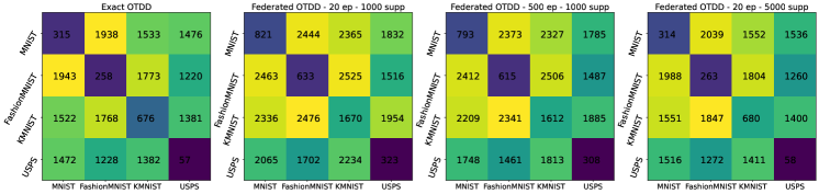
Figure 6: Comparison of the matrix of distances between digits datasets computed by FedWaD and the true OTDD distance between the same datasets. (left) OTDD, (middle-left) FedWaD with $20$ epochs and $1000$ support points, (middle-right) FedWaD with $500$ epochs and $1000$ support points, (right) FedWaD with $20$ epochs and $5000$ support points

Boosting FL methods

One of the challenges in FL is the heterogeneity of the data distribution among clients. This heterogeneity is usually due to shift in class-conditional distributions or to a label shift (some classes being absent on a client). As such, we propose to investigate a simple approach that allows to address dataset heterogeneity (in terms of distributions) among clients, by leveraging on our ability to compute distance between datasets in a federated way.

Our proposal involves computing pairwise dataset distances between clients, clustering them based on their (di)-similarities using a spectral clustering algorithm (Von Luxburg, 2007), and using this clustering knowledge to enhance existing federated learning algorithms. In our approach, we run the FL algorithm for each of the $K$ clusters of clients instead of all clients to avoid information exchange between clients with diverse datasets. For example, for FedAvg, this means learning a global model for each cluster of clients, resulting in $K$ global models. For personalized models like FedRep (Collins et al., 2021), or FedPer (Arivazhagan et al., 2019), we run the personalized algorithm on each cluster of clients. By running FL algorithms on clustered client, we ensure information exchange only between similar clients and improves the overall performance of federated learning algorithms by reducing the statistical dataset heterogeneity among clients.

We have run experiments on MNIST and CIFAR10 in which client datasets hold a clear cluster structure. We have also run experiments where there is no cluster structure in which clients are randomly assigned a pair of classes. In practice, we used the code of FedRep Collins et al. (2021) for the FedAvg, FedRep and FedPer and the spectral clustering method of scikit-learn (Pedregosa et al., 2011) (details are in Section D.5). Results are reported in Table 1 (with details in Section D.5). We can see that when there is a clear clustering structure among the clients, FedWaD is able to recover it and always improve the performance of the original federated learning algorithms. Depending on the algorithm, the improvement can be highly significant. For instance, for FedRep, the performance can be improved by $9$ points for CIFAR10 and up to $29$ for MNIST.   Interestingly, even without clear clustering structure, FedWaD is able to almost always improve the performance of all federated learning algorithms (except for some specific cases of FedPer). Again for FedRep, the performance uplift can reach $19$ points for CIFAR10 and $36$ for MNIST. In terms of clustering, the “affinity" parameter of the spectral clustering algorithm seems to be the most efficient and robust one.

Table 1: MNIST/CIFAR10 Average performances over 5 trials of three FL algorithms, FedAvg, FedRep and FedPer. For each algorithm we compare the vanilla performance with the ones obtained after clustering the clients using the FedWaD OTDD distance and three different setting of the spectral clustering algorithm (details in Appendix) and for a support size of $10$. The number of clients varies from $20$ to $100$. Bolded number indicate the best performing approach (and clustering parameters).

	Strong structure					No structure
		Clustering					Clustering
	Vanilla	Affinity	Sparse G. (3)	Sparse G. (5)		Vanilla	Affinity	Sparse G. (3)	Sparse G. (5)
MNIST
FedAvg
20	26.3 $\pm$ 3.8	99.5 $\pm$ 0.0	99.5 $\pm$ 0.0	91.5 $\pm$ 10.3		25.1 $\pm$ 6.6	71.3 $\pm$ 7.3	59.5 $\pm$ 3.0	57.0 $\pm$ 4.4
40	39.1 $\pm$ 9.0	99.2 $\pm$ 0.1	91.1 $\pm$ 6.5	94.5 $\pm$ 9.4		42.5 $\pm$ 10.5	70.8 $\pm$ 13.5	60.0 $\pm$ 3.7	58.1 $\pm$ 6.3
100	39.2 $\pm$ 7.7	98.9 $\pm$ 0.0	95.9 $\pm$ 4.6	98.4 $\pm$ 0.8		52.6 $\pm$ 3.9	64.4 $\pm$ 9.6	76.3 $\pm$ 5.4	67.9 $\pm$ 6.0
FedRep
20	81.1 $\pm$ 8.1	99.1 $\pm$ 0.0	99.1 $\pm$ 0.0	98.2 $\pm$ 1.3		75.6 $\pm$ 9.3	87.5 $\pm$ 4.5	81.4 $\pm$ 8.6	85.3 $\pm$ 7.3
40	88.8 $\pm$ 10.4	98.9 $\pm$ 0.1	93.3 $\pm$ 7.1	96.7 $\pm$ 4.5		78.0 $\pm$ 6.3	88.0 $\pm$ 4.3	78.9 $\pm$ 7.9	76.7 $\pm$ 5.6
100	93.0 $\pm$ 3.9	98.6 $\pm$ 0.1	98.4 $\pm$ 0.1	98.5 $\pm$ 0.1		86.0 $\pm$ 4.8	91.6 $\pm$ 3.1	89.1 $\pm$ 5.0	86.3 $\pm$ 4.9
FedPer
20	94.3 $\pm$ 4.3	99.5 $\pm$ 0.0	99.5 $\pm$ 0.0	99.3 $\pm$ 0.3		90.5 $\pm$ 2.4	92.7 $\pm$ 1.5	93.0 $\pm$ 4.3	93.8 $\pm$ 2.9
40	94.7 $\pm$ 7.6	99.2 $\pm$ 0.1	99.1 $\pm$ 0.2	97.9 $\pm$ 2.7		92.3 $\pm$ 1.3	90.2 $\pm$ 4.7	87.7 $\pm$ 4.1	89.2 $\pm$ 2.3
100	98.1 $\pm$ 0.1	98.9 $\pm$ 0.0	98.8 $\pm$ 0.2	98.9 $\pm$ 0.0		96.6 $\pm$ 0.9	96.6 $\pm$ 1.6	92.1 $\pm$ 3.3	90.2 $\pm$ 4.9
Average Uplift	-	26.4 $\pm$ 27.5	24.4 $\pm$ 26.5	24.4 $\pm$ 25.6		-	12.7 $\pm$ 14.6	8.7 $\pm$ 12.7	7.2 $\pm$ 11.4
CIFAR10
FedAvg
20	22.0 $\pm$ 2.6	75.1 $\pm$ 6.2	42.6 $\pm$ 4.5	52.2 $\pm$ 8.8		23.5 $\pm$ 6.9	71.4 $\pm$ 9.7	42.5 $\pm$ 4.7	49.7 $\pm$ 4.7
40	26.1 $\pm$ 7.1	65.9 $\pm$ 7.1	36.7 $\pm$ 18.3	48.8 $\pm$ 8.3		26.6 $\pm$ 5.1	73.4 $\pm$ 15.9	36.3 $\pm$ 4.5	32.3 $\pm$ 11.6
100	26.4 $\pm$ 4.3	68.0 $\pm$ 5.1	37.4 $\pm$ 11.4	39.8 $\pm$ 8.0		27.5 $\pm$ 2.0	54.6 $\pm$ 10.1	27.6 $\pm$ 4.1	29.0 $\pm$ 3.8
FedRep
20	81.8 $\pm$ 1.8	88.1 $\pm$ 2.0	84.4 $\pm$ 0.5	85.3 $\pm$ 0.5		85.3 $\pm$ 2.0	90.7 $\pm$ 2.5	87.9 $\pm$ 2.0	88.1 $\pm$ 1.4
40	80.3 $\pm$ 0.8	83.7 $\pm$ 2.0	81.0 $\pm$ 2.1	81.6 $\pm$ 1.7		84.1 $\pm$ 0.8	93.6 $\pm$ 2.9	84.8 $\pm$ 1.7	84.3 $\pm$ 0.5
100	75.0 $\pm$ 0.9	79.4 $\pm$ 2.3	75.2 $\pm$ 2.4	75.4 $\pm$ 1.5		77.9 $\pm$ 1.4	91.4 $\pm$ 2.0	77.8 $\pm$ 1.7	79.0 $\pm$ 1.1
FedPer
20	85.4 $\pm$ 2.3	91.0 $\pm$ 1.9	87.2 $\pm$ 0.5	87.8 $\pm$ 0.9		88.7 $\pm$ 1.7	92.3 $\pm$ 1.8	89.8 $\pm$ 2.0	90.1 $\pm$ 1.5
40	85.9 $\pm$ 0.8	87.2 $\pm$ 2.2	82.7 $\pm$ 2.5	84.3 $\pm$ 1.9		88.1 $\pm$ 0.7	94.8 $\pm$ 2.6	86.0 $\pm$ 2.3	84.9 $\pm$ 3.3
100	82.2 $\pm$ 0.4	85.1 $\pm$ 1.8	80.3 $\pm$ 2.0	80.9 $\pm$ 1.7		85.1 $\pm$ 0.6	94.0 $\pm$ 1.4	82.0 $\pm$ 2.4	83.0 $\pm$ 1.1
Average Uplift	-	17.6 $\pm$ 19.6	4.7 $\pm$ 7.3	7.9 $\pm$ 10.9		-	18.8 $\pm$ 16.6	3.1 $\pm$ 6.6	3.7 $\pm$ 8.3

5 Conclusion

In this paper, we presented a principled approach for computing the Wasserstein distance between two distributions in a federated manner. Our proposed algorithm, called FedWaD, leverages the geometric properties of the Wasserstein distance and associated geodesics to estimate the distance while respecting the privacy of the samples stored on different devices. We established the convergence properties of FedWaD and provided empirical evidence of its practical effectiveness through simulations on various problems, including dataset distance and coreset computation. Our approach shows potential applications in the fields of machine learning and privacy-preserving data analysis, where computing distances for distributed data is a fundamental task.

Appendix A Property of the approximating interpolating measure

Theorem 1.

Assume that $\mu$ and $\xi^{(k)}$ are two discrete distributions with the same number of samples $n$ and uniform weights., Then for any $t$, the approximating interpolating measure given by equation Equation 10 is equal to the exact one Equation 5.

Proof.

Remind that the approximating interpolating measure is defined as

$$\xi_{t}=\frac{1}{n}\sum_{i=1}^{n}\delta_{(1-t)x_{i}+tn(\mathbf{P}^{\star}\mathbf{X}^{\prime})_{i}}$$ (11)

whereas the exact interpolating measure is defined as

$$\mu_{t}=\sum_{i,j}^{n,m}\mathbf{P}_{i,j}^{\star}\delta_{(1-t)x_{i}+tx_{j}^{\prime}}$$ (12)

where $\mathbf{P}^{\star}$ is the optimal transportation plan between $\xi$ and $\xi^{\prime}$, $x_{i}$ and $x_{j}^{\prime}$ are the samples from these distributions and $\mathbf{X}^{\prime}$ is the matrix of samples from $\xi^{\prime}$. Because $\mu$ and $\xi^{(k)}$ have the same number of samples $n$ and uniform weights, $\mathbf{P}^{\star}$ is a weighted (by $1/n$) permutation matrix Peyré et al. (2019). Let us denote by $\sigma$ the permutation associated to $\mathbf{P}^{\star}$. Then, for the approximation, we have

$$\xi_{t} =\frac{1}{n}\sum_{i=1}^{n}\delta_{(1-t)x_{i}+tn(\mathbf{P}^{\star}\mathbf{X}^{\prime})_{i}}$$

$$=\frac{1}{n}\sum_{i=1}^{n}\delta_{(1-t)x_{i}+tx_{\sigma(i)}^{\prime}}$$

$$=\sum_{i=1}^{n}\frac{1}{n}\delta_{(1-t)x_{i}+tx_{\sigma(i)}^{\prime}}$$

$$=\mu_{t}$$

where the last equality comes from the fact that for each row $i$, $P_{i,j}^{\star}$ is non-zero only for $\sigma(i)$ column and $P_{i,\sigma(i)}^{\star}=1/n$. ∎

Appendix B Proof of Theorem 2

Theorem 2.

Let $\mu$ and $\nu$ be two measures in $\mathscr{P}_{p}(X)$. For $k\in\mathbb{N}$, let $\xi_{\mu}^{(k)}$, $\xi_{\nu}^{(k)}$ and $\xi^{(k)}$ be interpolating measures computed at iteration $k$ as defined in Algorithm 1. Define

$$A^{(k)}=\mathcal{W}_{p}(\mu,\xi_{\mu}^{(k)})+\mathcal{W}_{p}(\xi_{\mu}^{(k)},\xi^{(k)})+\mathcal{W}_{p}(\xi^{(k)},\xi_{\nu}^{(k)})+\mathcal{W}_{p}(\xi_{\nu}^{(k)},\nu)$$

Then, the sequence $(A^{(k)})$ is non-increasing and converges to $\mathcal{W}_{p}(\mu,\nu)$.

Proof.

First, remind that $\xi_{\mu}^{(k)}$ and $\xi_{\nu}^{(k)}$ are the interpolating measures between $\mu$ and $\xi^{(k-1)}$ and between $\xi^{(k-1)}$ and $\nu$ respectively, as defined in Algorithm 1. Likewise, $\xi_{\mu}^{(k+1)}$ and $\xi_{\nu}^{(k+1)}$ are interpolating measures between $\mu$ and $\xi^{(k)}$ and between $\xi^{(k)}$ and $\nu$ respectively. Hence, we have

$$\mathcal{W}_{p}(\mu,\xi_{\mu}^{(k+1)})+\mathcal{W}_{p}(\xi_{\mu}^{(k+1)},\xi^{(k)})\leq\mathcal{W}_{p}(\mu,\xi_{\mu}^{(k)})+\mathcal{W}_{p}(\xi_{\mu}^{(k)},\xi^{(k)})$$

and

$$\mathcal{W}_{p}(\nu,\xi_{\nu}^{(k+1)})+\mathcal{W}_{p}(\xi_{\nu}^{(k+1)},\xi^{(k)})\leq\mathcal{W}_{p}(\nu,\xi_{\nu}^{(k)})+\mathcal{W}_{p}(\xi_{\nu}^{(k)},\xi^{(k)})$$

These two inequalities lead to,

$$\mathcal{W}_{p}(\mu,\xi_{\mu}^{(k+1)})+\mathcal{W}_{p}(\xi_{\mu}^{(k+1)},\xi^{(k)})+\mathcal{W}_{p}(\nu,\xi_{\nu}^{(k+1)})+\mathcal{W}_{p}(\xi_{\nu}^{(k+1)},\xi^{(k)})$$

$$\leq\mathcal{W}_{p}(\mu,\xi_{\mu}^{(k)})+\mathcal{W}_{p}(\xi_{\mu}^{(k)},\xi^{(k)})+\mathcal{W}_{p}(\nu,\xi_{\nu}^{(k)})+\mathcal{W}_{p}(\xi_{\nu}^{(k)},\xi^{(k)})$$

Besides, since $\xi^{(k+1)}$ is an interpolating measure between $\xi_{\mu}^{(k+1)}$ and $\xi_{\nu}^{(k+1)}$, we have

$$\mathcal{W}_{p}(\xi_{\mu}^{(k+1)},\xi^{(k+1)})+\mathcal{W}_{p}(\xi^{(k+1)},\xi_{\nu}^{(k+1)})\leq\mathcal{W}_{p}(\xi_{\mu}^{(k+1)},\xi^{(k)})+\mathcal{W}_{p}(\xi^{(k)},\xi_{\nu}^{(k+1)})$$

and

$$A^{(k+1)}\leq A^{(k)}$$

Hence, the sequence $(A^{(k)})$ is non-increasing. Additionally, by the triangle inequality, we have for any $k\in\mathbb{N}$,

$$\mathcal{W}_{p}(\mu,\nu)\leq A^{(k)}$$

We conclude by using the monotone convergence theorem: since $(A^{(k)})$ is non-increasing and bounded sequence below, then it converges to its infimum.

We now justify why the limit of $(A^{(k)})$ is $\mathcal{W}_{p}(\mu,\nu)$. At convergence, we have reached a stationary point in the $(A^{(k)})$,

$$\lim_{k\to+\infty}A^{(k)} =\mathcal{W}_{p}(\mu,\xi_{\mu}^{(\infty)})+\mathcal{W}_{p}(\xi_{\mu}^{(\infty)},\xi^{(\infty)})+\mathcal{W}_{p}(\xi^{(\infty)},\xi_{\nu}^{(\infty)})+\mathcal{W}_{p}(\xi_{\nu}^{(\infty)},\nu)$$

however there are an infinite number of triplets $(\xi_{\mu}^{(k)},\xi_{\nu}^{(k)},\xi^{(k)})$ that allow to reach this value by the nature of the algorithm. By definition, $\xi_{\mu}^{(\infty)}$ and $\xi_{\nu}^{(\infty)}$ are interpolating measures between $\mu$ and $\xi^{(\infty)}$ and between $\xi^{(\infty)}$ and $\nu$ respectively. Hence, by choosing $t=0$ and $t=1$ in the definition of the interpolating measure, we have $\xi_{\mu}^{(\infty)}=\mu$ and $\xi_{\nu}^{(\infty)}=\nu$. Therefore, $\xi^{(\infty)}$ is also an interpolating measure between $\mu$ and $\nu$ as belonging to the geodesic between $\mu$ and $\nu$. Then, we have

$$\lim_{k\to+\infty}A^{(k)} =\mathcal{W}_{p}(\mu,\xi_{\mu}^{(\infty)})+\mathcal{W}_{p}(\xi_{\mu}^{(\infty)},\xi^{(\infty)})+\mathcal{W}_{p}(\xi^{(\infty)},\xi_{\nu}^{(\infty)})+\mathcal{W}_{p}(\xi_{\nu}^{(\infty)},\nu)$$

$$=\mathcal{W}_{p}(\mu,\xi^{(\infty)})+\mathcal{W}_{p}(\xi^{(\infty)},\nu)$$

$$=\mathcal{W}_{p}(\mu,\nu)$$

where the first equality results from the fact that $\xi_{\mu}^{(\infty)}$ and $\xi_{\nu}^{(\infty)}$ are interpolating measures between $\mu$ and $\xi^{(\infty)}$ and between $\xi^{(\infty)}$ and $\nu$ respectively and the second equality is obtained from the fact that $\xi^{(\infty)}$ is also an interpolating measure between $\mu$ and $\nu$ as belonging to the geodesic between $\mu$ and $\nu$. ∎

Let us note that the convergence of the algorithm requires choosing $\xi_{\mu}^{(\infty)}=\mu$ and $\xi_{\nu}^{(\infty)}=\nu$ thus leaking the client distributions to the server. However, this is just a theoretical argument that we use just to show that the algorithm converges so that $\lim_{k\to+\infty}A^{(k)}=\mathcal{W}_{p}(\mu,\nu)$. In practice, we avoid setting $t=0$ and $t=1$ in the definition of the interpolating measures.

Appendix C Convergence rate of the algorithm for Gaussian distributions with same covariance

In this section, we show that when $\mu$ and $\nu$ are Gaussians after one iteration, we can infer $W(\mu,nu)$ and the sequence of iterates $(\xi^{(k)})$ obtained for $t=0.5$ converges to the $\xi^{\star}$ the interpolating measure between $\mu$ and $\nu$ for $t=0.5$

Theorem 3.

Assume that $\mu$, $\nu$ and $\xi^{(0)}$ are three Gaussian distributions with the same covariance matrix $\Sigma$ ie $\mu\sim\mathcal{N}(\mathbf{m}_{\mu},\Sigma)$, $\nu\sim\mathcal{N}(\mathbf{m}_{\nu},\Sigma)$ and $\xi^{(0)}\sim\mathcal{N}(\mathbf{m}_{\xi^{(0)}},\Sigma)$. Further assume that we are not in the trivial case where $\mathbf{m}_{\mu}$, $\mathbf{m}_{\nu}$, and $\mathbf{m}_{\xi^{(0)}}$ are aligned. Applying our algorithm Algorithm 1 with $t=0.5$ and the squared Euclidean cost, we have the following properties:

1. all interpolating measures $\xi_{\mu}^{(k)}$,$\xi_{\nu}^{(k)}$, $\xi^{(k)}$ are isotropic Gaussian distributions with the same covariance matrix $\Sigma$

2. for any $k\geq 1$, $\mathcal{W}_{2}(\mu,\nu)=\|\mathbf{m}_{\mu}-\mathbf{m}_{\nu}\|_{2}=2\|\mathbf{m}_{\xi_{\mu}^{(k)}}-\mathbf{m}_{\xi_{\nu}^{(k)}}\|_{2}$

3. $\mathcal{W}_{2}(\xi^{(k)},\xi^{\star})=\frac{1}{2}\mathcal{W}_{2}(\xi^{(k-1)},\xi^{\star})$

4. $\mathcal{W}_{2}(\mu,\xi^{(k)})+\mathcal{W}_{2}(\xi^{(k)},\nu)-\mathcal{W}_{2}(\mu,\nu)\leq\frac{1}{2^{k-1}}\mathcal{W}_{2}(\xi^{(0)},\xi^{(\star)})$

Proof.

The first point comes from the fact that Wasserstein barycenter of Gaussians are Gaussians Agueh & Carlier (2011); Peyré et al. (2019). For isotropic Gaussians with same covariance, the covariance matrice of the barycenter remains unchanged while the mean is the barycenter mean. So, in our case, the interpolating measure with $t=0.5$ i.e the uniform barycenter of two measures, say $\mu$ and $\xi^{(k-1)}$, is $\xi_{\mu}^{(k)}\sim\mathcal{N}(\mathbf{m}_{\xi_{\mu}^{(k)}},\Sigma)$, where $\mathbf{m}_{\xi_{\mu}^{(k)}}=\frac{1}{2}(\mathbf{m}_{\mu}+\mathbf{m}_{\xi^{(k-1)}})$. The consequence of this first point of the theorem is that since we are going to deal with same covariance Gaussian distributions, then the Wasserstein distance between any pair of measures involved in our algorithm only depends on the Euclidean distance of their means and we will use interchangeably the Euclidean distance and the Wasserstein distance.  
 
The second point is proven by using geometrical arguments in the plane $(P)$ in which the three points, for $k\geq 1$, $\mathbf{m}_{\mu}$, $\mathbf{m}_{\nu}$, $\mathbf{m}_{\xi^{(k-1)}}$ lie (note that based on our assumption, this plane always exists). By definition of $\xi_{\mu}^{(k)}$ and $\xi_{\nu}^{(k)}$ and given the above point, we have

$$\mathbf{m}_{\xi_{\mu}^{(k)}}=\frac{1}{2}(\mathbf{m}_{\mu}+\mathbf{m}_{\xi^{(k-1)}})\quad\text{and}\quad\mathbf{m}_{\xi_{\nu}^{(k)}}=\frac{1}{2}(\mathbf{m}_{\nu}+\mathbf{m}_{\xi^{(k-1)}})$$

By using the intercept theorem, since $t=\frac{1}{2}$, in the plane $(P)$, the segment $[\mathbf{m}_{\xi_{\mu}^{(k)}},\mathbf{m}_{\xi_{\nu}^{(k)}}]$ is parallel to the segment $[\mathbf{m}_{\mu},\mathbf{m}_{\nu}]$ and we have :

$$\frac{1}{2}=\frac{\|\mathbf{m}_{\xi_{\mu}^{(k)}}-\mathbf{m}_{\xi{(k-1)}}\|_{2}}{\|\mathbf{m}_{\mu}-\mathbf{m}_{\xi{(k-1)}}\|_{2}}=\frac{\|\mathbf{m}_{\xi_{\nu}^{(k)}}-\mathbf{m}_{\xi{(k-1)}}\|_{2}}{\|\mathbf{m}_{\nu}-\mathbf{m}_{\xi{(k-1)}}\|_{2}}==\frac{\|\mathbf{m}_{\xi_{\nu}^{(k)}}-\mathbf{m}_{\xi_{\mu}^{(k)}}\|_{2}}{\|\mathbf{m}_{\nu}-\mathbf{m}_{\mu}\|_{2}}$$

which gives us the second point.  
 
For the third point, we are going to consider geometrical arguments similar as above. However, we are going to first show that for a given $k$, the mid point, denoted as $\hat{\xi}^{(k)}$, between $\xi^{(k-1)}$ and $\xi^{\star}$ is also $\xi^{(k)}$ as defined by our algorithm.

By definition, $\xi^{\star}$ is the mid point interpolating measure between $\mu$ and $\nu$, whose mean is $\frac{1}{2}(\mathbf{m}_{\mu}+\mathbf{m}_{\nu})$. Since $\hat{\xi}^{(k)}$ and $\xi_{\mu}^{(k)}$ are respectively the mid point measure between $\xi^{(k-1)}$ and $\xi^{\star}$ and $\mu$ and $\xi^{(k-1)}$, we can apply the intercept theorem in the appropriate plane and get

$$W_{2}(\hat{\xi}^{(k)},\xi_{\mu}^{(k)})=\frac{1}{2}W_{2}(\mu,\xi^{\star})$$

Using a similar reasoning using $\nu$, we get

$$W_{2}(\hat{\xi}^{(k)},\xi_{\nu}^{(k)})=\frac{1}{2}W_{2}(\nu,\xi^{\star})$$

Summing these two equations, we obtain

$$W_{2}(\hat{\xi}^{(k)},\xi_{\mu}^{(k)})+W_{2}(\hat{\xi}^{(k)},\xi_{\nu}^{(k)})=\frac{1}{2}W_{2}(\mu,\xi^{\star})+\frac{1}{2}W_{2}(\nu,\xi^{\star})=\frac{1}{2}W_{2}(\mu,\nu)=W_{2}(\xi_{\mu}^{(k)},\xi_{\nu}^{(k)})$$

where the second equality comes from the fact that $\xi^{\star}$ is an interpolant measure of $\mu$ and $\nu$, while the last equality comes from the second point of the theorem.

Hence, since we have $W_{2}(\hat{\xi}^{(k)},\xi_{\mu}^{(k)})+W_{2}(\hat{\xi}^{(k)},\xi_{\nu}^{(k)})=W_{2}(\xi_{\mu}^{(k)},\xi_{\nu}^{(k)})$, it also mean than

$$\hat{\xi}^{(k)}\in\mathop{\mathrm{arg\,min}}_{\xi}\frac{1}{2}W_{2}(\xi_{\mu}^{(k)},\xi)+\frac{1}{2}W_{2}(\xi,\xi_{\nu}^{(k)})$$

and $\hat{\xi}^{(k)}$ is also the midpoint interpolating measure between $\xi_{\mu}^{(k)}$ and $\xi_{\nu}^{(k)}$.

Then, applying the intercept theorem with $\xi^{(k-1)}$, $\xi^{(k)}$, $\xi^{\star}$, $\mu$ and $\xi_{\mu}^{(k)}$, we obtain the desired result

$$\frac{1}{2}W_{2}(\xi^{(k-1)},\xi^{\star})=W_{2}(\xi^{(k)},\xi^{\star})$$

Finally, given all the above, it is simple to show the convergence rate of the algorithm using simple triangle inequalities.

$$\mathcal{W}_{2}(\mu,\xi^{(k)})+\mathcal{W}_{2}(\xi^{(k)},\nu)-\mathcal{W}_{2}(\mu,\nu) \leq \mathcal{W}_{2}(\mu,\xi^{\star})+\mathcal{W}_{2}(\xi^{\star},\xi^{(k)})+\mathcal{W}_{2}(,\xi^{(k)},\xi^{\star})+\mathcal{W}_{2}(\xi^{\star},\nu)-\mathcal{W}_{2}(\mu,\nu)$$

$$= 2\mathcal{W}_{2}(\xi^{(k)},\xi^{\star})$$

$$= \frac{1}{2^{k-1}}\mathcal{W}_{2}(\xi^{(0)},\xi^{\star})$$

∎

Figure 7: Illustration of the geometrical interpretation of the algorithm and its convergence proof for Gaussian distributions with same covariance, based on the intercept theorem.

Appendix D Additional experiments

D.1 Toy Analysis : the impact of approximating the interpolating measure

We propose to analyze in this section the benefits and disadvantages of approximating the interpolating measure instead of using the exact one as given in Equation 5. For this purpose, we compare the running time and the accuracy of the exact Wasserstein distance, our exact FedWaD, and our approximate FedWaD for estimating the Wasserstein distance between two Gaussians distributions. The Gaussians are different means but same covariances so that the true Wasserstein distance is known and equal to the Euclidean distance between the means. We have considered two different settings ($d=2$ and $d=50$) of Gaussians dimensionality. For the first case ($d=2$), we detail the results presented in the main paper. Note that when the dimensionality of the Gaussians are set to $50$, we do not expect the Wasserstein distance nor FedWaD to provide a good estimation of the closed form distance between these distributions, due to the curse of dimensionality of the Wasserstein distance (Fournier & Guillin, 2015)

As default parameter for our approximate FedWaD, we considered $20$ iterations and a support of size $10$, then we varied the number of samples $n$ from $10$ to $10000$. We have run experiments in different settings

• we analyzed the impact of sample ratio between the two distributions, as this may impact the support size of the approximating interpolating measure accross FedWaD iterations.

• we made varying the support size of the approximating interpolating measure at fixed sample ratio.

Results have been averaged over $10$ runs.

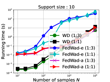
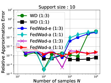
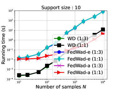
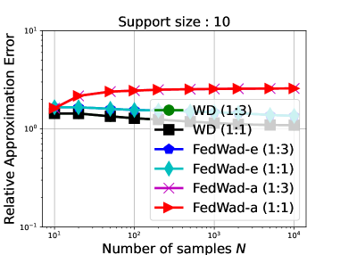
Figure 8: For different sample ratios, (1:3) or (1:1), in the two distributions we report the performance of the different models. For our approximated FedWaD, we have set the support size to $10$. (top) $d=2$ (bottom) $d=50$. (left) running time. (right) relative error.

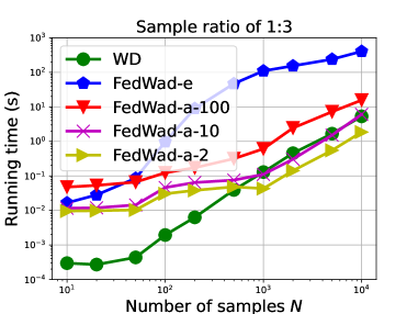
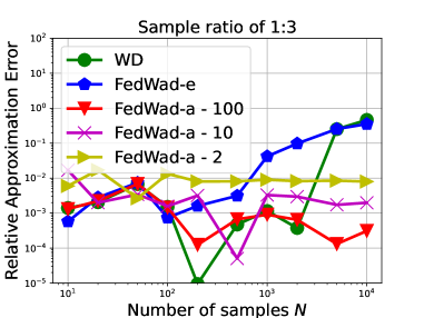
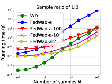
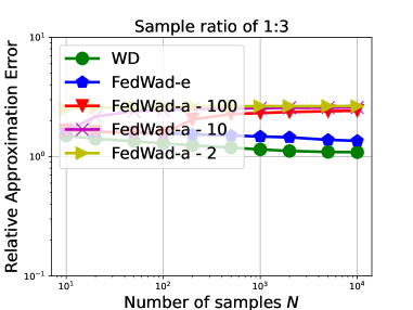
Figure 9: For increasing number of samples, we report (top) $d=2$ (bottom) $d=50$. (left) Running time of the Wasserstein distance, our exact FedWaD and our approximate FedWaD. (right) the relative error of the different models : the computed Wasserstein distance, our exact FedWaD and the approximated FedWad with a support size of $10$ and $100$. The first distribution has a number of samples $N$ and the second ones $N/3$.

Analyzing the impact of sample ratio

Given the setting with uniform weights, when the sample ratio is $1$, the optimal plan is theoretically a scaled permutation matrix. Hence, the support size of the exact interpolating measure is expected, in theory, to be fixed and equal to $N$. When the ratio of samples is different to $1$, the support size of the exact interpolating may increase at each iteration of the algorithm and leads to a larger running time. Figure 8 - left panel - shows the running time of all compared methods as well as their relative error - right panel - compared to the true Wasserstein distance. We note that for $2d$ Gaussians, both the Wasserstein distance and our approximated FedWaD with support size of $10$ the running time is increasing with a natural computational overhead for the 1:1 sample ratio (as we have more samples). For the exact FedWaD, the behavior is different. the running time for the 1:3 sample ratio is larger than the 1:1. This is due to the optimal transportation plan $\mathbf{P}^{\star}$ not being exactly a scaled permutation matrix. As a result, the support size of the interpolating measure increases with the number of samples, leading to computational overhead for the method. For $50d$ Gaussians, the differences in running time between the different sample ratio are negligible.

In the case of $2d$ Gaussians (top row), For the relative error, for $N<1000$, we note that all methods achieve similar errors. Numerical errors start to appear for exact FedWaD and the Wasserstein distance for respectively $N\geq 1000$ and $N\geq 5000$ depending on the sample ratio. Interestingly, the approximated FedWaD is robust to large number of samples and achieves similar errors as for small number of samples. For higher dimensions (bottom row), all the methods are not able to provide accurate estimation of the Wasserstein distance and with the worst relative error for the approximated FedWaD with a support size of $10$. Nonetheless, we want to emphasize that despite this lack of accuracy, the approximated FedWaD can be useful in high-dimension problems as we have shown for the other experiments.

Analyzing the support size of approximated interpolating measure

Figure 9 shows the running time and the relative error of the different methods for a sample ratio of $1:3$ and when the support sizes of the approximating interpolating measure are $2$,$10$ or $100$. We clearly remark the computational cost of a larger support size with a benefit in terms of approximation error appearing mostly when $N\geq 1000$ and for small dimension problems (top row). For higher dimension problems (bottom row), we see again the benefit on running time of the approximated approach, yet with a larger approximation error.

D.2 Details on Coreset and additonal results

Experimental setting

We sampled $20000$ examples randomly from the MNIST dataset, and dispatched them at random on $100$ clients but such that only a subset $K$ of the $10$ classes is present on each client. We learn $10$ coresets over $1000$ epochs and at each epoch, we assume that only $10$ random clients are available and can be used for computing FedWaD. For FedWaD, the support size of the interpolating measure has been set to either $10$ or $100$ and the number of iteration in FedWaD to $20$.

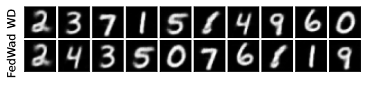
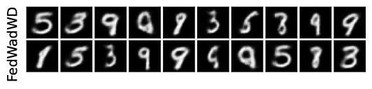
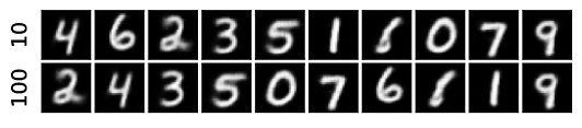
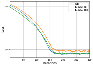
Figure 10: Examples of the $10$ coreset obtained with for each panel (top-row) the exact Wasserstein and (bottow-row) FedWaD for the MNIST dataset. Different panels correspond to different number of classes $K$ on each client: (top) $K=8$, (middle) $K=2$, (bottom) support of the interpolating measure varying from $10$ to $100$. As class diversity on each client increases, the coreset is less effective at capturing the $10$ modes of the dataset

We have reproduced in here the same MNIST experiment (which results are reproduced in Figure 10) on coreset for the FashionMNIST dataset, and we can notice, in Figure 11 that we obtain similar results as for the MNIST dataset. When the number of shared classes $K$ is large enough, the coreset is not able to capture the different modes in the dataset. And again, we remark that the support size of the approximate interpolating measure has few impacts on the result. For both datasets, the loss landscape of the coreset learning reveals that our FedWaD-based approaches yield to a worse minimum than the exact Wasserstein distance, which is mostly due to the interpolating measure approximation. Figure 12 plots the performance of a nearest neighbor classifier based on the coresets learnt from each client for varying number of clients. Results show that coreset-based approaches are competitive, especially for high number of clients, with personalized FL algorithms, which are known to be the best performing FL algorithms in practice.

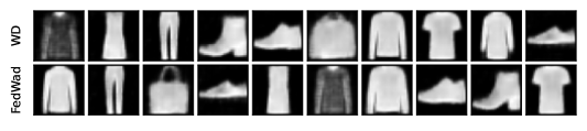
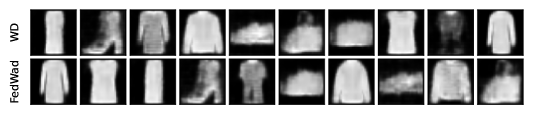
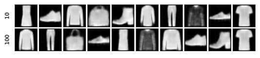
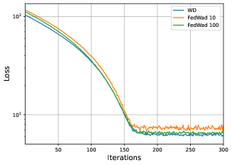
Figure 11: Examples of the $10$ coreset obtained with for each panel (top-row) the exact Wasserstein and (bottow-row), our FedWaD for the FashionMNIST dataset. Different panels correspond to different number of classes $K$ on each client: (top) $K=8$, (middle) $K=2$, (bottom) support of the interpolating measure for $K=8$.

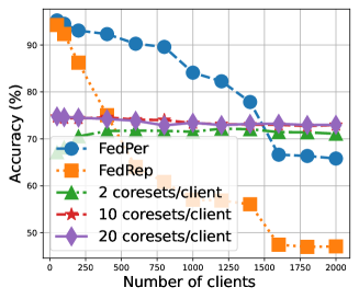
Figure 12: FashionMNIST performance of a nearest neighbor classifier based on the coresets learnt from each client for varying number of clients and number of coresets per clients We have compared to the performance of two personalized FL algorithms.

D.3 Details on Federated OTDD experiments

Geometric dataset distances via federated Wasserstein distance.

Transfer learning and domain adaptation are important ML paradigms, which aim at transferring knowledge across similar domains. The main underlying concept in these approaches is the notion of distance or similarity between datasets. Transferring knowledge between comparable domains is typically simpler than between distant ones. In certain applications, it is relevant to find datasets from which one can transfer knowledge from without disclosing the target dataset. This may be the case, for instance, in applications with low-resource clients storing sensitive data. In this case, the practitioner may want to find a dataset similar enough to the client’s dataset, in order to transfer knowledge from it. In practice, a server would train a classifier on a dataset that is similar to the client dataset, and the client would then use this classifier to perform inference on its own data.

In that context, our goal is to propose a distance between datasets that can be computed in a federated way based on FedWaD. We leverage the distance proposed in Alvarez-Melis & Fusi (2020), which is based on the Wasserstein distance between two labeled datasets $\mathcal{D}$ and $\mathcal{D}^{\prime}$. The ground metric is defined by,

$$d_{\mathcal{D}}((x,y),(x^{\prime},y^{\prime}))\triangleq(d(x,x^{\prime})+\mathcal{W}_{2}^{2}(\alpha_{y},\alpha_{y}^{\prime}))^{1/2}$$ (13)

where $d$ is a distance between two features $x$ and $x^{\prime}$, and $\alpha_{y}$ is the class-conditional distribution of $x$ given $y$. In order to reduce computational complexity, Alvarez-Melis & Fusi (2020) assume the class-conditionals are Gaussian, so that $\mathcal{W}_{2}$ boils down the $2$-Bures-Wasserstein distance, which is available in closed form:

$$\mathcal{W}_{2}^{2}(\alpha_{y},\alpha_{y^{\prime}})=\|m_{y}-m_{y^{\prime}}\|_{2}^{2}+\|\Sigma_{y}-\Sigma_{y^{\prime}}\|_{F}^{2}$$ (14)

where $m_{z}$ and $\Sigma_{z}$ denote the mean and covariance of $\alpha_{z}$.

FedWaD needs vectorial representations of the data to compute intermediate measures. The Bures-Wasserstein distance allows us to conveniently represent $\alpha_{y}$ as the concatenation of the mean $m_{y}$ and vectorized covariance $\Sigma_{y}$. Hence, we can compute the distance between two datasets $\mathcal{D}$ and $\mathcal{D}^{\prime}$ by augmenting each example from those datasets with the corresponding class-conditional mean and vectorized covariance, and using the $\ell_{2}$ norm as the ground metric in the Wasserstein distance. One can eventually reduce the dimension the augmented representation by considering only the diagonal of the covariance matrix.

D.4 Federated OTDD analysis

To evaluate our procedure, we replicated the experiments of Alvarez-Melis & Fusi (2020) on the dataset selection for transfer learning: given a source dataset, the goal is to find a target one which is the most similar to the source. We considered four real datasets, namely MNIST, KMNIST, USPS and FashionMNIST. We first analyze the impact of two hyperparameters, the number of epochs and the number of support points in the interpolating measure, on the distance computation between $5000$ samples from MNIST and KMNIST, Figure 13 shows the evolution of the distance between MNIST and KMNIST as well as the running time for varying values of hyperparameters. The number of epochs has a very small impact on the distance and using $10$ epochs suffices to get a reasonably accurate approximation of the distance. On the other hand, the number of support point seems more critical, and we need at least $5000$ support points to obtain a very accurate approximation, although we have a nice linear convergence of the distance with respect to support size.

We also analyzed the impact of the dataset size on the distance computation and running time: Figure 14 shows the evolution of the distance and the running time with respect to the the sample size in the two distributions. We note that the order relation is preserved between the two distances for all possible range of sample size. Another interesting observation is that as long as the sample size is smaller than the support size of the interpolating measure, FedWaD provides an accurate estimation of the distance. When the sample size is larger then the distance is overestimated. This is due to a less accurate estimation of an exact interpolating measure (which is supported on $2n+1$ points). Regarding computational efficiency, we observe that for small support size of the interpolating measure, the running time increases at the same rate as the sample size, whereas for larger support size, the running time increases $10$-fold for an $100$-fold increase in sample size.

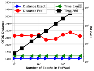
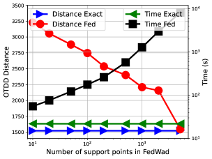
Figure 13: FedWaD and OTDD distances on MNIST-KMNIST and its running time against (left) the number of epochs and (right) the number of support points in the interpolating measure. For each plot, the left and right $y$-axis report the distance and the running time respectively.

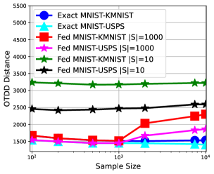
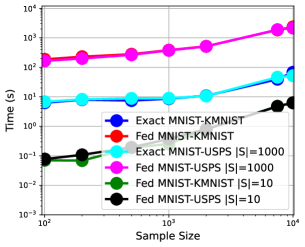
Figure 14: (left) Distance and (right) running time against the dataset size for the MNIST-KMNIST an MNIST-USPS distances, for varying number of support points $|S|$

D.5 Boosting FL methods

We provide here more detailed results about our experiments on boosting FL methods. Figure 15 shows the distance matrices obtained for MNIST and CIFAR10 when the number of clients is $20$ for different structures on the clients datasets. We can clearly see the cluster structure on the MNIST dataset when it exists, but when there is no structure, the distance matrix is more uniform yet show some variations For CIFAR10, no clear structure is visible on the distance matrix as the dataset is more complex. Nonetheless, our experiments on boosting FL methods show that even in this case, clustering c lients can help improve the performances of federated learning algorithms.

Those distance matrices are the one we use as the input of the spectral clustering algorithm. We used the spectral clustering algorithm of scikit-learn (Pedregosa et al., 2011) with the following setting::

• we denoted as “affinity", the setting in which the distance matrix, after rescaling, is used as affinity matrix, where larger values indicate greater similarity between instances. (see affinity parameter set to ‘precomputed’ In scikit-learn)

• we denote as Sparse G. (3) and Sparse G. (5) the setting in which the distance matrix is interpreted as a sparse graph of distances, and construct a binary affinity matrix from the ($3$ or $5$) nearest neighbors of each instance. matrix is computed

Details on the cluster structure

We have built this cluster structure on the client datasets by assigning to each client one pair of classes among the following $5$ ones : $[(0,1),(2,3),(4,5),(6,7),(8,9)]$. When the number of clients in equal to $10$, each cluster is composed of $2$ clients. For a larger number of clients, each cluster is of random size with a minimum of $2$ clients.

Practical algorithmic details

In practice, we used the code of FedRep Collins et al. (2021) for the FedAvg, FedRep and FedPer and the spectral clustering method of scikit-learn Pedregosa et al. (2011). The federated OT distance dataset has been computed on the original data space while for CIFAR10, we have worked on the 784-dimensional code obtained from an (untrained) randomly initialized autoencoder. We have also considered the case where the there is no specific clustering structure on the clients as they randomly select a pair of classes among the $10$ ones.

Extra results

Performance results on federated learning are reported below for different settings. Table 2 and Table 3 show the results for MNIST respectively with and without client structure. Table 4 and Table 5 report similar results for CIFAR10.

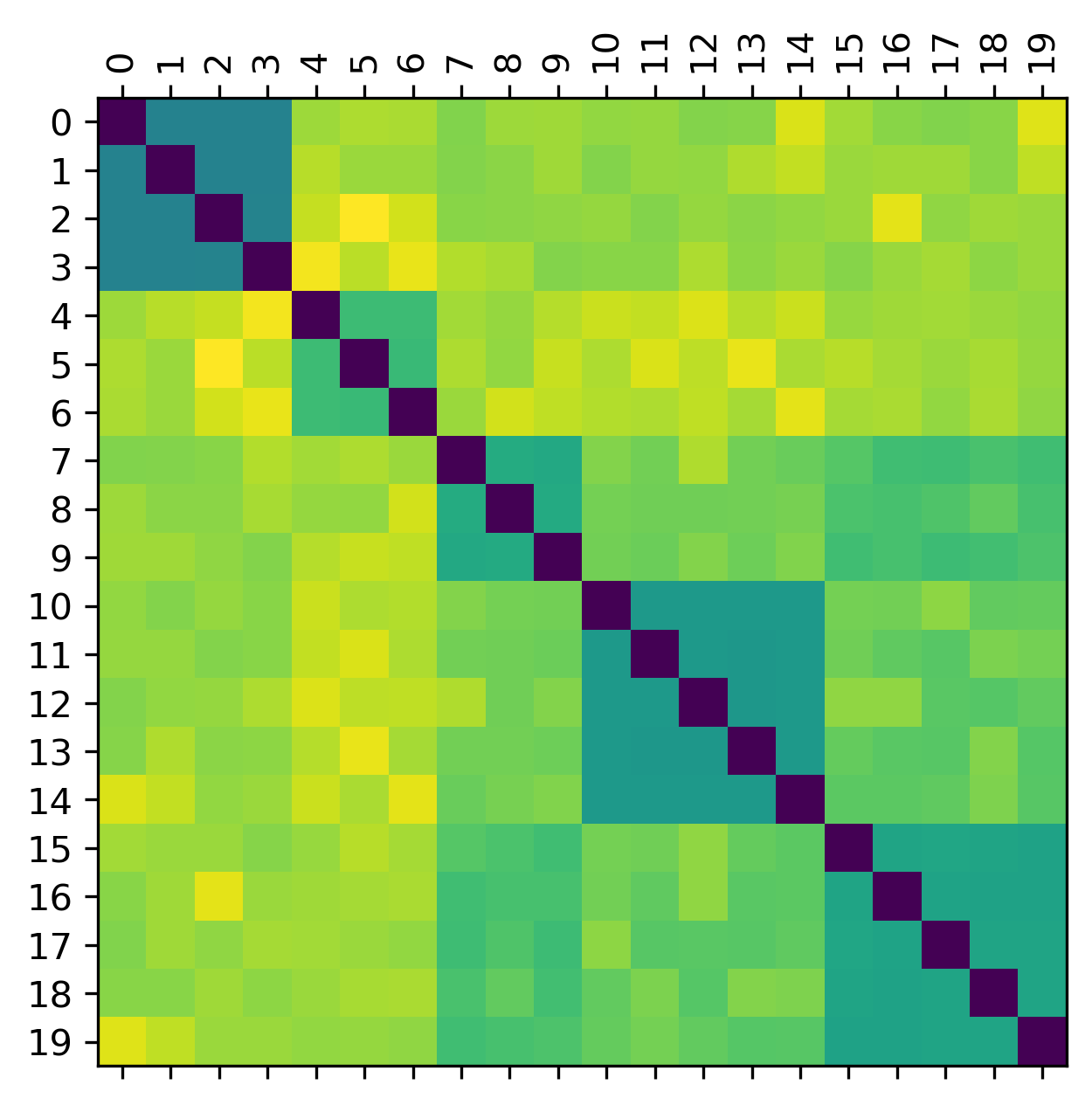
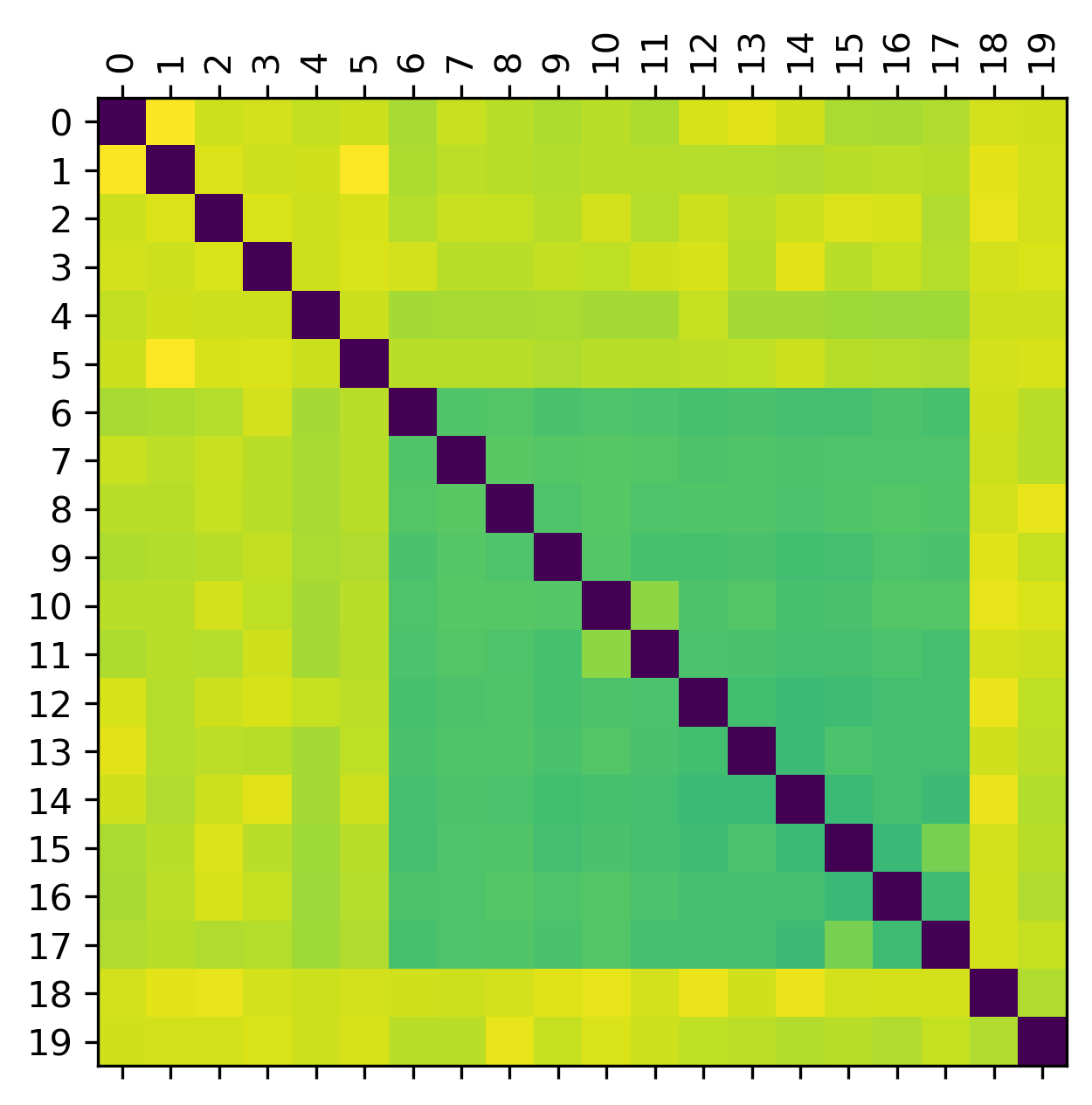
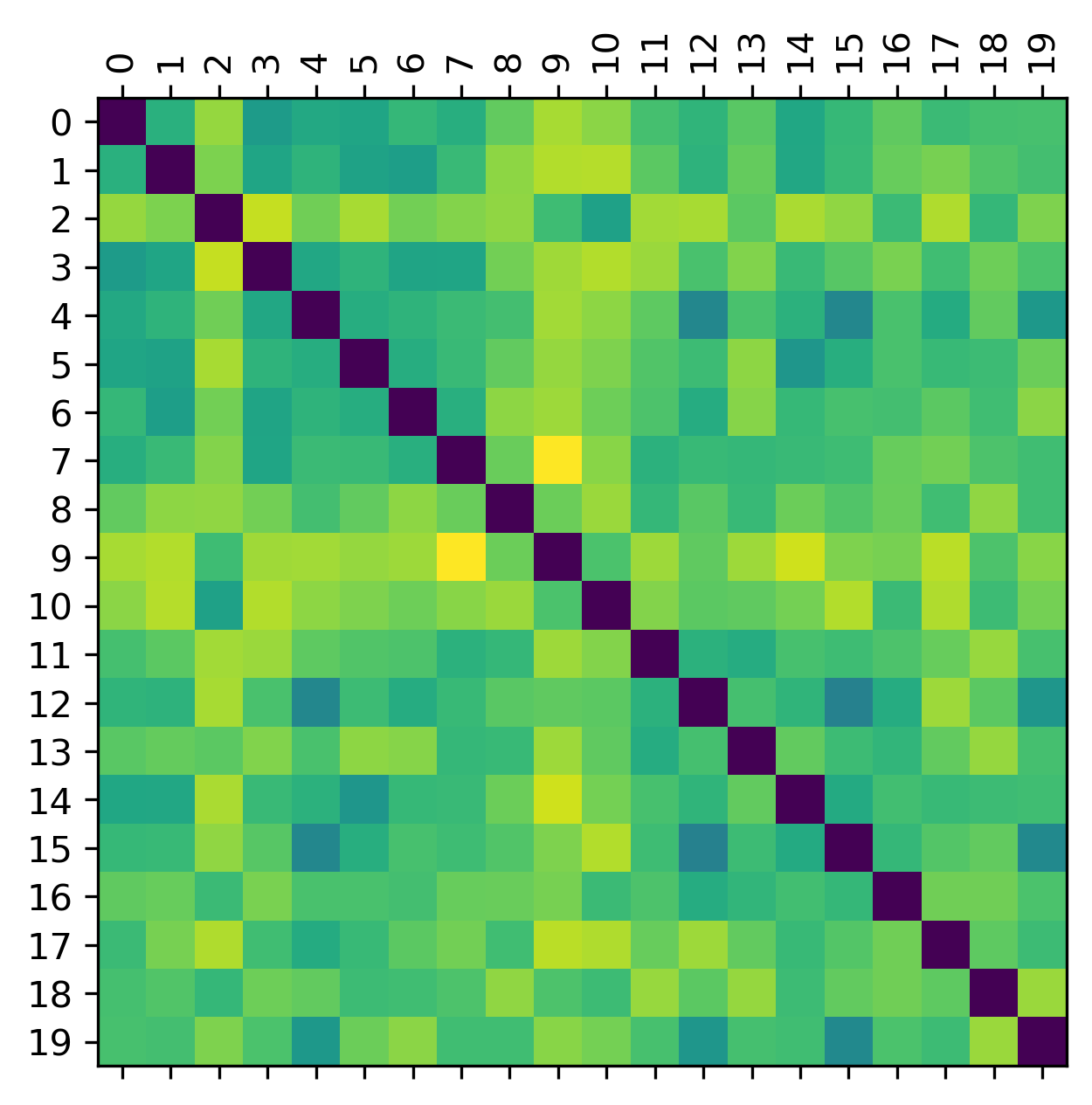
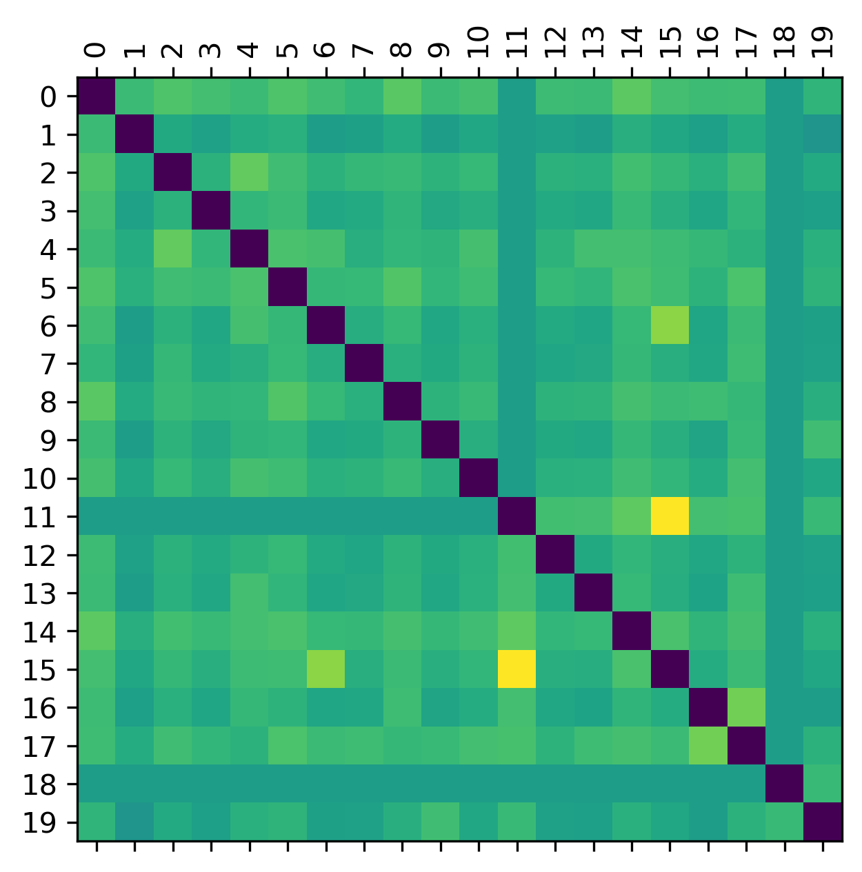
Figure 15: (left) MNIST and (right) CIFAR10 distance matrices for $20$ clients computed using our Federated OTDD . On the top row, we have imposed a cluster structure on client datasets while on the bottom row, there is no specific sructure. We can note that this structure is clearly visible on the MNIST dataset but less on CIFAR10. Eventhough, clustering clients will help improve federated learning algorithm performances.

		Clustered
		Affinity		Sparse G. (3)		Sparse G. (5)
	Vanilla	10	100	10	100	10	100
FedAvg
10	19.6 $\pm$ 0.9	99.6 $\pm$ 0.0	99.6 $\pm$ 0.0	90.5 $\pm$ 8.7	91.8 $\pm$ 9.6	84.5 $\pm$ 8.0	85.2 $\pm$ 5.7
20	26.3 $\pm$ 3.8	99.5 $\pm$ 0.0	99.5 $\pm$ 0.0	99.5 $\pm$ 0.0	99.5 $\pm$ 0.0	91.5 $\pm$ 10.3	96.5 $\pm$ 6.0
40	39.1 $\pm$ 9.0	99.2 $\pm$ 0.1	99.2 $\pm$ 0.1	91.1 $\pm$ 6.5	99.2 $\pm$ 0.1	94.5 $\pm$ 9.4	99.2 $\pm$ 0.1
100	39.2 $\pm$ 7.7	98.9 $\pm$ 0.0	98.9 $\pm$ 0.0	95.9 $\pm$ 4.6	96.7 $\pm$ 3.8	98.4 $\pm$ 0.8	98.9 $\pm$ 0.0
FedRep
10	71.6 $\pm$ 10.5	99.4 $\pm$ 0.0	99.4 $\pm$ 0.1	94.3 $\pm$ 7.7	99.0 $\pm$ 0.5	95.5 $\pm$ 5.6	90.5 $\pm$ 6.6
20	81.1 $\pm$ 8.1	99.1 $\pm$ 0.0	99.1 $\pm$ 0.1	99.1 $\pm$ 0.0	99.1 $\pm$ 0.0	98.2 $\pm$ 1.3	99.0 $\pm$ 0.2
40	88.8 $\pm$ 10.4	98.9 $\pm$ 0.1	98.9 $\pm$ 0.0	93.3 $\pm$ 7.1	99.0 $\pm$ 0.1	96.7 $\pm$ 4.5	99.0 $\pm$ 0.1
100	93.0 $\pm$ 3.9	98.6 $\pm$ 0.1	98.6 $\pm$ 0.1	98.4 $\pm$ 0.1	98.4 $\pm$ 0.1	98.5 $\pm$ 0.1	98.5 $\pm$ 0.1
FedPer
10	86.7 $\pm$ 4.3	99.6 $\pm$ 0.0	99.6 $\pm$ 0.0	99.5 $\pm$ 0.1	99.6 $\pm$ 0.1	98.4 $\pm$ 2.0	98.9 $\pm$ 1.0
20	94.3 $\pm$ 4.3	99.5 $\pm$ 0.0	99.5 $\pm$ 0.0	99.5 $\pm$ 0.0	99.5 $\pm$ 0.0	99.3 $\pm$ 0.3	99.5 $\pm$ 0.0
40	94.7 $\pm$ 7.6	99.2 $\pm$ 0.1	99.2 $\pm$ 0.1	99.1 $\pm$ 0.2	99.2 $\pm$ 0.1	97.9 $\pm$ 2.7	99.2 $\pm$ 0.1
100	98.1 $\pm$ 0.1	98.9 $\pm$ 0.0	98.9 $\pm$ 0.0	98.8 $\pm$ 0.2	98.8 $\pm$ 0.1	98.9 $\pm$ 0.0	98.9 $\pm$ 0.0
Average Uplift	-	29.8 $\pm$ 28.4	29.8 $\pm$ 28.4	27.2 $\pm$ 26.6	29.0 $\pm$ 27.2	26.7 $\pm$ 25.2	27.6 $\pm$ 26.3

Table 2: MNIST Average performances over 5 trials of three FL algorithms: FedAvg, FedRep and FedPer. For each algorithm we compare the vanilla performance with the ones obtained after clustering the clients using the FedOTDD distance, using three different parameters of the spectral clustering algorithm and for a support size of $10$ and $100$. The number of clients varies from $10$ to $100$. For this table, datasets from clients do have a clear cluster structure

		Clustered
		Affinity		Sparse G. (3)		Sparse G. (5)
	Vanilla	10	100	10	100	10	100
FedAvg
10	20.2 $\pm$ 0.6	81.0 $\pm$ 4.2	81.3 $\pm$ 4.5	78.0 $\pm$ 6.0	77.7 $\pm$ 6.6	71.5 $\pm$ 5.1	72.0 $\pm$ 6.0
20	25.1 $\pm$ 6.6	71.3 $\pm$ 7.3	72.0 $\pm$ 4.3	59.5 $\pm$ 3.0	59.5 $\pm$ 5.7	57.0 $\pm$ 4.4	60.5 $\pm$ 2.3
40	42.5 $\pm$ 10.5	70.8 $\pm$ 13.5	70.3 $\pm$ 13.3	60.0 $\pm$ 3.7	59.5 $\pm$ 10.6	58.1 $\pm$ 6.3	56.9 $\pm$ 6.1
100	52.6 $\pm$ 3.9	64.4 $\pm$ 9.6	60.4 $\pm$ 11.3	76.3 $\pm$ 5.4	68.2 $\pm$ 6.1	67.9 $\pm$ 6.0	65.4 $\pm$ 3.7
FedRep
10	54.3 $\pm$ 11.2	90.1 $\pm$ 6.7	90.1 $\pm$ 7.5	92.1 $\pm$ 4.2	91.8 $\pm$ 4.6	91.0 $\pm$ 4.4	94.0 $\pm$ 3.1
20	75.6 $\pm$ 9.3	87.5 $\pm$ 4.5	86.1 $\pm$ 2.6	81.4 $\pm$ 8.6	85.1 $\pm$ 6.3	85.3 $\pm$ 7.3	87.1 $\pm$ 5.5
40	78.0 $\pm$ 6.3	88.0 $\pm$ 4.3	85.4 $\pm$ 4.8	78.9 $\pm$ 7.9	74.9 $\pm$ 8.7	76.7 $\pm$ 5.6	79.6 $\pm$ 5.7
100	86.0 $\pm$ 4.8	91.6 $\pm$ 3.1	90.7 $\pm$ 3.7	89.1 $\pm$ 5.0	84.5 $\pm$ 2.9	86.3 $\pm$ 4.9	84.9 $\pm$ 3.6
FedPer
10	82.0 $\pm$ 10.1	98.4 $\pm$ 1.4	96.5 $\pm$ 3.5	96.4 $\pm$ 3.5	96.5 $\pm$ 3.6	98.5 $\pm$ 1.4	98.3 $\pm$ 1.3
20	90.5 $\pm$ 2.4	92.7 $\pm$ 1.5	95.4 $\pm$ 0.5	93.0 $\pm$ 4.3	96.2 $\pm$ 3.0	93.8 $\pm$ 2.9	94.5 $\pm$ 2.5
40	92.3 $\pm$ 1.3	90.2 $\pm$ 4.7	91.0 $\pm$ 4.9	87.7 $\pm$ 4.1	87.0 $\pm$ 3.7	89.2 $\pm$ 2.3	87.5 $\pm$ 5.4
100	96.6 $\pm$ 0.9	96.6 $\pm$ 1.6	96.4 $\pm$ 2.0	92.1 $\pm$ 3.3	93.0 $\pm$ 2.3	90.2 $\pm$ 4.9	86.9 $\pm$ 1.7
Average Uplift	-	18.9 $\pm$ 18.9	18.3 $\pm$ 19.2	15.7 $\pm$ 18.6	14.8 $\pm$ 18.6	14.1 $\pm$ 17.1	14.3 $\pm$ 18.1

Table 3: MNIST Average performances over 5 trials of three FL algorithms: FedAvg, FedRep and FedPer. For each algorithm we compare the vanilla performance with the ones obtained after clustering the clients using the FedOTDD distance, using three different parameters of the spectral clustering algorithm and for a support size of $10$ and $100$. The number of clients varies from $10$ to $100$. For this table, datasets from clients do not have a clear cluster structure

		Clustered
		Affinity		Sparse G. (3)		Sparse G. (5)
	Vanilla	10	100	10	100	10	100
FedAvg
10	17.6 $\pm$ 1.1	79.1 $\pm$ 6.3	78.6 $\pm$ 6.0	61.6 $\pm$ 2.6	69.5 $\pm$ 5.1	72.2 $\pm$ 9.4	72.3 $\pm$ 6.0
20	22.0 $\pm$ 2.6	75.1 $\pm$ 6.2	66.9 $\pm$ 9.1	42.6 $\pm$ 4.5	52.4 $\pm$ 17.0	52.2 $\pm$ 8.8	56.2 $\pm$ 13.6
40	26.1 $\pm$ 7.1	65.9 $\pm$ 7.1	70.1 $\pm$ 5.7	36.7 $\pm$ 18.3	46.2 $\pm$ 15.7	48.8 $\pm$ 8.3	49.9 $\pm$ 12.1
100	26.4 $\pm$ 4.3	68.0 $\pm$ 5.1	68.3 $\pm$ 4.7	37.4 $\pm$ 11.4	44.9 $\pm$ 13.0	39.8 $\pm$ 8.0	43.1 $\pm$ 10.4
Fedrep
10	82.4 $\pm$ 2.3	91.1 $\pm$ 1.2	90.7 $\pm$ 1.2	89.4 $\pm$ 0.8	90.3 $\pm$ 1.0	89.7 $\pm$ 2.3	90.0 $\pm$ 1.1
20	81.8 $\pm$ 1.8	88.1 $\pm$ 2.0	85.9 $\pm$ 1.4	84.4 $\pm$ 0.5	86.0 $\pm$ 2.1	85.3 $\pm$ 0.5	86.8 $\pm$ 1.4
40	80.3 $\pm$ 0.8	83.7 $\pm$ 2.0	86.2 $\pm$ 0.9	81.0 $\pm$ 2.1	82.3 $\pm$ 2.5	81.6 $\pm$ 1.7	82.1 $\pm$ 1.4
100	75.0 $\pm$ 0.9	79.4 $\pm$ 2.3	78.5 $\pm$ 1.7	75.2 $\pm$ 2.4	76.3 $\pm$ 1.6	75.4 $\pm$ 1.5	76.9 $\pm$ 1.1
FedPer
10	82.1 $\pm$ 2.3	93.2 $\pm$ 1.1	93.0 $\pm$ 0.8	91.7 $\pm$ 0.5	93.0 $\pm$ 0.8	92.3 $\pm$ 2.0	92.7 $\pm$ 1.0
20	85.4 $\pm$ 2.3	91.0 $\pm$ 1.9	89.1 $\pm$ 1.8	87.2 $\pm$ 0.5	88.7 $\pm$ 2.5	87.8 $\pm$ 0.9	89.5 $\pm$ 1.9
40	85.9 $\pm$ 0.8	87.2 $\pm$ 2.2	89.7 $\pm$ 1.4	82.7 $\pm$ 2.5	85.4 $\pm$ 2.7	84.3 $\pm$ 1.9	84.9 $\pm$ 1.6
100	82.2 $\pm$ 0.4	85.1 $\pm$ 1.8	83.4 $\pm$ 2.7	80.3 $\pm$ 2.0	81.3 $\pm$ 1.8	80.9 $\pm$ 1.7	82.5 $\pm$ 1.5
Average Uplift	-	20.0 $\pm$ 21.3	19.4 $\pm$ 20.8	8.6 $\pm$ 12.5	12.4 $\pm$ 15.1	11.9 $\pm$ 16.0	13.3 $\pm$ 16.1

Table 4: CIFAR10 Average performances over 5 trials of three FL algorithms: FedAvg, FedRep and FedPer. For each algorithm we compare the vanilla performance with the ones obtained after clustering the clients using the FedOTDD distance, using three different parameters of the spectral clustering algorithm and for a support size of $10$ and $100$. The number of clients varies from $10$ to $100$. For this table, datasets from clients do have cluster structure

		Clustered
		Affinity		Sparse G. (3)		Sparse G. (5)
	Vanilla	10	100	10	100	10	100
FedAvg
10	18.1 $\pm$ 0.7	71.3 $\pm$ 7.3	71.0 $\pm$ 3.4	72.7 $\pm$ 6.2	72.6 $\pm$ 4.1	76.6 $\pm$ 2.6	72.4 $\pm$ 1.6
20	23.5 $\pm$ 6.9	71.4 $\pm$ 9.7	71.2 $\pm$ 7.9	42.5 $\pm$ 4.7	47.8 $\pm$ 4.8	49.7 $\pm$ 4.7	44.4 $\pm$ 8.1
40	26.6 $\pm$ 5.1	73.4 $\pm$ 15.9	71.1 $\pm$ 15.0	36.3 $\pm$ 4.5	30.9 $\pm$ 7.1	32.3 $\pm$ 11.6	30.3 $\pm$ 4.6
100	27.5 $\pm$ 2.0	54.6 $\pm$ 10.1	54.6 $\pm$ 10.2	27.6 $\pm$ 4.1	29.8 $\pm$ 6.8	29.0 $\pm$ 3.8	28.3 $\pm$ 5.6
FedRep
10	83.6 $\pm$ 2.2	90.3 $\pm$ 3.1	90.3 $\pm$ 2.4	91.2 $\pm$ 1.6	91.1 $\pm$ 1.8	91.1 $\pm$ 2.7	91.2 $\pm$ 1.7
20	85.3 $\pm$ 2.0	90.7 $\pm$ 2.5	91.5 $\pm$ 2.6	87.9 $\pm$ 2.0	88.4 $\pm$ 2.2	88.1 $\pm$ 1.4	88.6 $\pm$ 1.8
40	84.1 $\pm$ 0.8	93.6 $\pm$ 2.9	93.3 $\pm$ 2.8	84.8 $\pm$ 1.7	84.4 $\pm$ 0.7	84.3 $\pm$ 0.5	85.3 $\pm$ 1.2
100	77.9 $\pm$ 1.4	91.4 $\pm$ 2.0	91.6 $\pm$ 1.9	77.8 $\pm$ 1.7	78.0 $\pm$ 2.4	79.0 $\pm$ 1.1	79.4 $\pm$ 1.7
FedPer
10	83.1 $\pm$ 2.1	92.6 $\pm$ 2.2	92.7 $\pm$ 1.4	93.0 $\pm$ 1.4	93.1 $\pm$ 1.5	93.0 $\pm$ 2.0	93.1 $\pm$ 1.3
20	88.7 $\pm$ 1.7	92.3 $\pm$ 1.8	92.7 $\pm$ 2.4	89.8 $\pm$ 2.0	90.2 $\pm$ 1.8	90.1 $\pm$ 1.5	90.0 $\pm$ 1.2
40	88.1 $\pm$ 0.7	94.8 $\pm$ 2.6	94.6 $\pm$ 2.5	86.0 $\pm$ 2.3	86.5 $\pm$ 0.7	84.9 $\pm$ 3.3	85.7 $\pm$ 1.4
100	85.1 $\pm$ 0.6	94.0 $\pm$ 1.4	94.1 $\pm$ 1.3	82.0 $\pm$ 2.4	82.3 $\pm$ 2.2	83.0 $\pm$ 1.1	83.6 $\pm$ 1.6
Average Uplift	-	19.9 $\pm$ 18.0	19.7 $\pm$ 17.5	8.3 $\pm$ 15.2	8.6 $\pm$ 15.4	9.1 $\pm$ 16.6	8.4 $\pm$ 15.1

Table 5: CIFAR10 Average performances over 5 trials of three FL algorithms: FedAvg, FedRep and FedPer. For each algorithm we compare the vanilla performance with the ones obtained after clustering the clients using the FedOTDD distance, using three different parameters of the spectral clustering algorithm and for a support size of $10$ and $100$. The number of clients varies from $10$ to $100$. For this table, datasets from clients do not have a clear cluster structure

References

- Agarwal et al. (2005) Pankaj K Agarwal, Sariel Har-Peled, Kasturi R Varadarajan, et al. Geometric approximation via coresets. Combinatorial and computational geometry, 52(1):1–30, 2005.
- Agueh & Carlier (2011) Martial Agueh and Guillaume Carlier. Barycenters in the wasserstein space. SIAM Journal on Mathematical Analysis, 43(2):904–924, 2011.
- Alvarez-Melis & Fusi (2020) David Alvarez-Melis and Nicolo Fusi. Geometric dataset distances via optimal transport. Advances in Neural Information Processing Systems, 33:21428–21439, 2020.
- Ambrosio et al. (2005) Luigi Ambrosio, Nicola Gigli, and Giuseppe Savaré. Gradient flows: in metric spaces and in the space of probability measures. Springer Science & Business Media, 2005.
- Arivazhagan et al. (2019) Manoj Ghuhan Arivazhagan, Vinay Aggarwal, Aaditya Kumar Singh, and Sunav Choudhary. Federated learning with personalization layers. arXiv preprint arXiv:1912.00818, 2019.
- Bauer et al. (2015) Martin Bauer, Sarang Joshi, and Klas Modin. Diffeomorphic density matching by optimal information transport. SIAM Journal on Imaging Sciences, 8(3):1718–1751, 2015.
- Claici et al. (2018) Sebastian Claici, Aude Genevay, and Justin Solomon. Wasserstein measure coresets. arXiv preprint arXiv:1805.07412, 2018.
- Collins et al. (2021) Liam Collins, Hamed Hassani, Aryan Mokhtari, and Sanjay Shakkottai. Exploiting Shared Representations for Personalized Federated Learning. In International Conference on Machine Learning, pp. 2089–2099, 2021.
- Courty et al. (2018) Nicolas Courty, Remi Flamary, and Melanie Ducoffe. Learning wasserstein embeddings. In International Conference on Learning Representations (ICLR), 2018.
- Fournier & Guillin (2015) Nicolas Fournier and Arnaud Guillin. On the rate of convergence in wasserstein distance of the empirical measure. Probability theory and related fields, 162(3-4):707–738, 2015.
- Gribonval et al. (2021) Remi Gribonval, Antoine Chatalic, Nicolas Keriven, Vincent Schellekens, Laurent Jacques, and Philip Schniter. Sketching data sets for large-scale learning: Keeping only what you need. IEEE Signal Processing Magazine, 38(5):12–36, 2021.
- Huguet et al. (2022) Guillaume Huguet, Daniel Sumner Magruder, Alexander Tong, Oluwadamilola Fasina, Manik Kuchroo, Guy Wolf, and Smita Krishnaswamy. Manifold interpolating optimal-transport flows for trajectory inference. Advances in Neural Information Processing Systems, 35:29705–29718, 2022.
- Kairouz et al. (2021) Peter Kairouz, H. Brendan McMahan, Brendan Avent, Aurélien Bellet, Mehdi Bennis, Arjun Nitin Bhagoji, K. A. Bonawitz, Zachary Charles, Graham Cormode, Rachel Cummings, Rafael G.L. D’Oliveira, Salim El Rouayheb, David Evans, Josh Gardner, Zachary Garrett, Adrià Gascón, Badih Ghazi, Phillip B. Gibbons, Marco Gruteser, Zaid Harchaoui, Chaoyang He, Lie He, Zhouyuan Huo, Ben Hutchinson, Justin Hsu, Martin Jaggi, Tara Javidi, Gauri Joshi, Mikhail Khodak, Jakub Konecny, Aleksandra Korolova, Farinaz Koushanfar, Sanmi Koyejo, Tancrède Lepoint, Yang Liu, Prateek Mittal, Mehryar Mohri, Richard Nock, Ayfer Özgür, Rasmus Pagh, Mariana Raykova, Hang Qi, Daniel Ramage, Ramesh Raskar, Dawn Song, Weikang Song, Sebastian U. Stich, Ziteng Sun, Ananda Theertha Suresh, Florian Tramèr, Praneeth Vepakomma, Jianyu Wang, Li Xiong, Zheng Xu, Qiang Yang, Felix X. Yu, Han Yu, and Sen Zhao. Advances and Open Problems in Federated Learning. Foundations and Trends in Machine Learning, 14(1–2):1–210, 2021.
- Kolouri et al. (2017) Soheil Kolouri, Se Rim Park, Matthew Thorpe, Dejan Slepcev, and Gustavo K Rohde. Optimal mass transport: Signal processing and machine-learning applications. IEEE signal processing magazine, 34(4):43–59, 2017.
- Lê Tien et al. (2019) Nam Lê Tien, Amaury Habrard, and Marc Sebban. Differentially private optimal transport: Application to domain adaptation. In IJCAI, pp. 2852–2858, 2019.
- Liu et al. (2021) Zhaorong Liu, Leye Wang, and Kai Chen. Secure efficient federated knn for recommendation systems. In Advances in Natural Computation, Fuzzy Systems and Knowledge Discovery, pp. 1808–1819. Springer, 2021.
- Maas et al. (2017) Jan Maas, Martin Rumpf, and Stefan Simon. Transport based image morphing with intensity modulation. In Scale Space and Variational Methods in Computer Vision: 6th International Conference, SSVM 2017, Kolding, Denmark, June 4-8, 2017, Proceedings, pp. 563–577. Springer, 2017.
- McMahan et al. (2017) Brendan McMahan, Eider Moore, Daniel Ramage, Seth Hampson, and Blaise Aguera y Arcas. Communication-efficient learning of deep networks from decentralized data. In Artificial intelligence and statistics, pp. 1273–1282. PMLR, 2017.
- Munteanu et al. (2018) Alexander Munteanu, Chris Schwiegelshohn, Christian Sohler, and David Woodruff. On coresets for logistic regression. Advances in Neural Information Processing Systems, 31, 2018.
- Pedregosa et al. (2011) F. Pedregosa, G. Varoquaux, A. Gramfort, V. Michel, B. Thirion, O. Grisel, M. Blondel, P. Prettenhofer, R. Weiss, V. Dubourg, J. Vanderplas, A. Passos, D. Cournapeau, M. Brucher, M. Perrot, and E. Duchesnay. Scikit-learn: Machine learning in Python. Journal of Machine Learning Research, 12:2825–2830, 2011.
- Peyré et al. (2019) Gabriel Peyré, Marco Cuturi, et al. Computational optimal transport: With applications to data science. Foundations and Trends® in Machine Learning, 11(5-6):355–607, 2019.
- Phillips (2016) Jeff M Phillips. Coresets and sketches. arXiv preprint arXiv:1601.00617, 2016.
- Schoppmann et al. (2018) Phillipp Schoppmann, Adrià Gascón, and Borja Balle. Private nearest neighbors classification in federated databases. IACR Cryptol. ePrint Arch., 2018:289, 2018.
- Von Luxburg (2007) Ulrike Von Luxburg. A tutorial on spectral clustering. Statistics and computing, 17:395–416, 2007.
- Wang et al. (2021) Jianyu Wang, Zachary Charles, Zheng Xu, Gauri Joshi, H. Brendan McMahan, Blaise Aguera y Arcas, Maruan Al-Shedivat, Galen Andrew, Salman Avestimehr, Katharine Daly, Deepesh Data, Suhas Diggavi, Hubert Eichner, Advait Gadhikar, Zachary Garrett, Antonious M. Girgis, Filip Hanzely, Andrew Hard, Chaoyang He, Samuel Horvath, Zhouyuan Huo, Alex Ingerman, Martin Jaggi, Tara Javidi, Peter Kairouz, Satyen Kale, Sai Praneeth Karimireddy, Jakub Konecny, Sanmi Koyejo, Tian Li, Luyang Liu, Mehryar Mohri, Hang Qi, Sashank J. Reddi, Peter Richtarik, Karan Singhal, Virginia Smith, Mahdi Soltanolkotabi, Weikang Song, Ananda Theertha Suresh, Sebastian U. Stich, Ameet Talwalkar, Hongyi Wang, Blake Woodworth, Shanshan Wu, Felix X. Yu, Honglin Yuan, Manzil Zaheer, Mi Zhang, Tong Zhang, Chunxiang Zheng, Chen Zhu, and Wennan Zhu. A Field Guide to Federated Optimization. arXiv preprint arXiv:2107.06917, 2021.
- Zhang et al. (2023) Kaining Zhang, Yongxin Tong, Yexuan Shi, Yuxiang Zeng, Yi Xu, Lei Chen, Zimu Zhou, Ke Xu, Weifeng Lv, and Zhiming Zheng. Approximate k-nearest neighbor query over spatial data federation. In Database Systems for Advanced Applications: 28th International Conference, DASFAA 2023, Tianjin, China, April 17–20, 2023, Proceedings, Part I, pp. 351–368. Springer, 2023.