ABSTRACT

To reduce the dimensionality of the functional covariate, functional principal component analysis plays a key role, however, there is uncertainty on the number of principal components. Model averaging addresses this uncertainty by taking a weighted average of the prediction obtained from a set of candidate models. In this paper, we develop an optimal model averaging approach that selects the weights by minimizing a $K$-fold cross-validation criterion. We prove the asymptotic optimality of the selected weights in terms of minimizing the excess final prediction error, which greatly improves the usual asymptotic optimality in terms of minimizing the final prediction error in the literature. When the true regression relationship belongs to the set of candidate models, we provide the consistency of the averaged estimators. Numerical studies indicate that in most cases the proposed method performs better than other model selection and averaging methods, especially for extreme quantiles.

Keywords: Functional data, model averaging, quantile regression, excess final prediction error, asymptotic optimality.

1 Introduction

Functional data analysis deals with data that are in the form of functions, which have become increasingly important over the past two decades. See, e.g., the monographs by Ramsay and Silverman, (2005), Ferraty and Vieu, (2006), Horváth and Kokoszka, (2012), Zhang, (2013), and Hsing and Eubank, (2015) and review articles by Cuevas, (2014), Morris, (2015), and Wang et al., (2016). This paper focuses on quantile regression for scalar responses and functional-valued covariates. Specifically, we investigate functional linear quantile regression (FLQR) model in which the conditional quantile for a fixed quantile index is modeled as a linear function of the functional covariate that has been introduced in Cardot et al., (2005). Since the seminal work of Koenker and Bassett, (1978), quantile regression has become one of the most important statistical methods in measuring the impact of covariates on response variables. An attractive feature of quantile regression is that it provides much more information about the conditional distribution of a response variable than the traditional mean regression. See Koenker, (2005) for a comprehensive review on quantile regression and its applications.

Functional quantile regression essentially extends the standard quantile regression framework to account for functional covariates, which has been extensively studied in the literature; see, for example, Cardot et al., (2005); Kato, (2012); Li et al., (2022); Ferraty et al., (2005); Chen and Müller, (2012). Cardot et al., (2005) considered a smoothing splines-based approach to represent the functional covariates for the FLQR model and established a convergence rate result. Kato, (2012) studied functional principal component analysis (FPCA)-based estimation for the FLQR model and established minimax optimal convergence rates for regression estimation and prediction. Li et al., (2022) and Sang et al., (2022) considered statistical inference for the FLQR model based on FPCA and reproducing kernel Hilbert space framework, respectively. Ferraty et al., (2005) and Chen and Müller, (2012) estimated the conditional quantile function by inverting the corresponding conditional distribution function. Yao et al., (2017) and Ma et al., (2019) studied a high-dimensional partially FLQR model that contains vector and functional-valued covariates.

Since functional data are often intrinsically infinite-dimensional, FPCA is a key dimension reduction tool for functional data analysis, which has been widely used in functional regression (Cai and Hall,, 2006; Yao et al., 2005b, ; Li et al.,, 2010; Kato,, 2012; Müller and Stadtmüller,, 2005). When using the FPCA approach to study functional regression, a crucial step is to select the number of principal components retained for the covariate. This essentially corresponds to a model selection problem, which aims to find the best model among a set of candidate models. A variety of model selection criteria have been proposed in functional regression, including the fraction of variance explained (FVE, Chen and Müller,, 2012), leave-one-curve-out cross-validation (Yao et al., 2005b, ; Kato,, 2012), the Akaike information criterion (AIC, Kato,, 2012; Müller and Stadtmüller,, 2005; Yao et al., 2005b, ), and the Bayesian information criterion (BIC, Kato,, 2012). More recently, Li et al., (2013) proposed various information criteria to select the number of principal components in functional data and established their consistency.

Model averaging combines a set of candidate models by taking a weighted average of them and can potentially reduce risk relative to model selection (Magnus et al.,, 2010; Yuan and Yang,, 2005; Peng and Yang,, 2022; Liu,, 2015; Liu and Okui,, 2013). Hansen and Racine, (2012) proposed jackknife (leave-one-out cross-validation) model averaging for least squares regression that selects the weights by minimizing a cross-validation criterion. Jackknife model averaging was further carried out on models with dependent data (Zhang et al.,, 2013) and linear quantile regression (Lu and Su,, 2015; Wang et al.,, 2023). Cheng and Hansen, (2015) extended the jackknife model averaging method to leave-$h$-out cross-validation criteria for forecasting in combination with factor-augmented regression, and Gao et al., (2016) further extended it to leave-subject-out cross-validation under a longitudinal data setting. Recently, the model averaging method has been developed for functional data analysis. For example, Zhang et al., (2018) developed a cross-validation model averaging estimator for functional linear regression in which both the response and the covariate are random functions. Zhang and Zou, (2020) proposed a jackknife model averaging method for a generalized functional linear model.

In this paper, we investigate the FLQR model using FPCA and model averaging methods. Instead of selecting the number of principal components (Kato,, 2012), we propose model averaging by taking a weighted average of the estimator or prediction obtained from a set of candidate models. In addition, we use the principal components analysis through conditional expectation technique (Yao et al., 2005a, ) to estimate functional principal component scores. Therefore, our method can deal with both sparsely and densely observed functional covariates. We select the model averaging weights by minimizing the $K$-fold cross-validation prediction error. We show that when there do not exist correctly specified models (i.e., true models) in the set of candidate models, the proposed method is asymptotically optimal in the sense that its excess final prediction error is as small as that of the infeasible best possible prediction. In particular, we find asymptotic optimality in the sense of minimizing the final prediction error, which is studied in the literature such as Lu and Su, (2015) and Wang et al., (2023), do not make much sense when there exists at least one true model in the set of candidate models. In the situation with true candidate models, we show that the averaged estimators for the model parameters are consistent. Our Monte Carlo simulations indicate the superiority of the proposed approach compared with other model averaging and selection methods for extreme quantiles. We apply our method to predict the quantile of the maximum hourly log-return of price of Bitcoin for a financial data.

The remainder of the paper is organized as follows. Section 2 presents the model and FPCA-based estimation and conditional quantile prediction. Section 3 proposes a model averaging procedure for conditional quantile prediction. Section 4 establishes the asymptotic properties of the resulting model averaging estimator. Section 5 conducts simulation studies to illustrate its finite sample performance. Section 6 applies the proposed method to a real financial data example. Section 7 concludes the paper. The proofs of the main results are relegated to the Supplementary Material.

2 Model and Estimation

2.1 Model Set-up

Let $\{(Y_{i},X_{i})\}_{i=1}^{n}$ be an independent and identically distributed (i.i.d.) sample, where $Y_{i}$ is a scalar random variable and $X_{i}=\{X_{i}(t):t\in\mathcal{T}\}$ is a random function defined on a compact interval $\mathcal{T}$ of $\mathbb{R}$. Let $Q_{\tau}(X_{i})$ denote the $\tau$th conditional quantile of $Y_{i}$ given $X_{i}$, where $\tau\in(0,1)$ is the quantile index. An FLQR model implies that $Q_{\tau}(X_{i})$ can be written as a linear functional of $X_{i}$, that is, there exist a scalar constant $a(\tau)\in\mathbb{R}$ and a slope function $b(\cdot,\tau)\in L_{2}(\mathcal{T})$ such that

$$Q_{\tau}(X_{i})=a(\tau)+\int_{\mathcal{T}}b(t,\tau)X_{i}^{c}(t)\,dt,$$ (2.1)

where $L_{2}(\mathcal{T})$ is the set of square-integrable functions defined on $\mathcal{T}$, $X_{i}^{c}(t)=X_{i}(t)-\mu(t)$, and $\mu(t)=E\{X_{i}(t)\}$ is the mean function of $X_{i}$. For notational simplicity, we suppress the dependence of $a(\tau)$ and $b(\cdot,\tau)$ on $\tau$. As a result, we have the following FLQR model

$$Y_{i}=Q_{\tau}(X_{i})+\varepsilon_{i}=a+\int_{\mathcal{T}}b(t)X_{i}^{c}(t)\,dt+\varepsilon_{i},$$

where $\varepsilon_{i}\equiv Y_{i}-Q_{\tau}(X_{i})$ satisfies the quantile restriction $P(\varepsilon_{i}\leq 0|X_{i})=\tau$ almost surely (a.s.).

Denote the covariance function of $X_{i}(t)$ by $G(s,t)=\mathrm{Cov}\{X_{i}(s),X_{i}(t)\}$. Since $G$ is a symmetric and nonnegative definite function, Mercer’s theorem (Hsing and Eubank,, 2015, Theorem 4.6.5) ensures that there exist a non-increasing sequence of eigenvalues $\kappa_{1}\geq\kappa_{2}\geq\cdots>0$ and a sequence of corresponding eigenfunctions $\{\phi_{j}\}_{j=1}^{\infty}$, such that

$$G(s,t)=\sum_{j=1}^{\infty}\kappa_{j}\phi_{j}(s)\phi_{j}(t).$$

Since $\{\phi_{j}\}_{j=1}^{\infty}$ is an orthonormal basis of $L_{2}(\mathcal{T})$, we have the following expansions in $L_{2}(\mathcal{T})$:

$$X_{i}^{c}(t)=\sum_{j=1}^{\infty}\xi_{ij}\phi_{j}(t),\quad b(t)=\sum_{j=1}^{\infty}b_{j}\phi_{j}(t),$$

where $b_{j}=\int_{\mathcal{T}}b(t)\phi_{j}(t)\,dt$ and $\xi_{ij}=\int_{\mathcal{T}}X_{i}^{c}(t)\phi_{j}(t)\,dt$. The $\xi_{ij}$’s are called functional principal component scores and satisfy $E(\xi_{ij})=0$, $E(\xi_{ij}^{2})=\kappa_{j}$, and $E(\xi_{ij}\xi_{ik})=0$ for all $j\neq k$. The expansion for $X_{i}^{c}(t)$ is called the Karhunen-Loève expansion (Hsing and Eubank,, 2015, Theorem 7.3.5). Then, the model (2.1) can be transformed into a linear quantile regression model with an infinite number of covariates:

$$Q_{\tau}(X_{i})=a+\sum_{j=1}^{\infty}b_{j}\xi_{ij}.$$ (2.2)

A nonlinear ill-posed inverse problem would be encountered when we want to fit the model (2.2) with a finite number of observations; see Kato, (2012) for a detailed discussion. We follow Kato, (2012) and address the ill-posed problem by truncating the model (2.2) to a feasible linear quantile regression model. It is common to keep only the first $J_{n}<\infty$ eigenbases, which leads to the following truncated model

$$Q_{\tau,J_{n}}(X_{i})=a+\sum_{j=1}^{J_{n}}b_{j}\xi_{ij},$$ (2.3)

where we allow $J_{n}$ to increase to infinity as $n\to\infty$ to reduce approximation errors. The regression parameters $a,b_{1},\ldots,b_{J_{n}}$ in model (2.3) need to be estimated.

2.2 FPCA-Based Quantile Prediction

In practice, we cannot observe the whole predictor trajectory $X_{i}(t)$. We typically assume that $X_{i}(t)$ can only be realized for some discrete set of sampling points with additional measurement errors, i.e., we observe data

$$U_{il}=X_{i}(T_{il})+\epsilon_{il},\quad T_{il}\in\mathcal{T};~{}l=1,\ldots,N_{i},$$ (2.4)

where $\epsilon_{il}$ are i.i.d. measurement errors with mean zero and finite variance $\sigma_{u}^{2}$, and $X_{i}(\cdot)$ are independent of $\epsilon_{il}$ ($i=1,\ldots,n$). Depending on the number of observations $N_{i}$ within each curve, functional data are typically classified as sparse and dense; see Li and Hsing, (2010) and Zhang and Wang, (2016) for details.

Many functions and parameters in the expressions given previously should be estimated from the data. We first use local linear smoothing to obtain the estimated mean function $\widehat{\mu}(t)$ and the estimated covariance function $\widehat{G}(s,t)$, which are well documented in the functional data analysis literature. For example, see Yao et al., 2005a ; Yao et al., 2005b , Li and Hsing, (2010), and Zhang and Wang, (2016) for the detailed calculations and we omit them here. Let the spectral decomposition of $\widehat{G}(s,t)$ be $\widehat{G}(s,t)=\sum_{j=1}^{\infty}\widehat{\kappa}_{j}\widehat{\phi}_{j}(s)\widehat{\phi}_{j}(t)$, where $\widehat{\kappa}_{1}\geq\widehat{\kappa}_{2}\geq\cdots\geq 0$ are the eigenvalues and $\{\widehat{\phi}_{1},\widehat{\phi}_{2},\ldots\}$ are corresponding eigenfunctions. When $X_{i}(t)$ are sparsely observed, $\xi_{ij}$ cannot be estimated by the integration formula. Here, we use the principal components analysis through conditional expectation (PACE) technique proposed by Yao et al., 2005a to obtain an estimate of $\xi_{ij}$. To be more specific, let $\mathbf{U}_{i}=(U_{i1},\ldots,U_{iN_{i}})^{\top}$, $\widehat{\bm{\phi}}_{ij}=\{\widehat{\phi}_{j}(T_{i1}),\ldots,\widehat{\phi}_{j}(T_{iN_{i}})\}^{\top}$, $\widehat{\bm{\mu}}_{i}=\{\widehat{\mu}(T_{i1}),\ldots,\widehat{\mu}(T_{iN_{i}})\}^{\top}$, and $\widehat{\mathbf{\Sigma}}_{\mathbf{U}_{i}}=\{\widehat{G}(T_{il},T_{il^{\prime}})+\widehat{\sigma}_{u}^{2}\delta_{ll^{\prime}}\}_{l,l^{\prime}=1}^{N_{i}}$, where $\widehat{\sigma}_{u}^{2}$ is an estimate of $\sigma_{u}^{2}$ and $\delta_{ll^{\prime}}=1$ if $l=l^{\prime}$ and 0 otherwise. Then, the PACE estimator of $\xi_{ij}$ is given by

$$\widehat{\xi}_{ij}=\widehat{\kappa}_{j}\widehat{\bm{\phi}}_{ij}^{\top}\widehat{\mathbf{\Sigma}}_{\mathbf{U}_{i}}^{-1}(\mathbf{U}_{i}-\widehat{\bm{\mu}}_{i}).$$ (2.5)

Note that this method can be applied to both sparsely and densely observed functional data. When $X_{i}(t)$ are densely observed, an alternative method is to use the “smoothing first, then estimation” procedure proposed by Ramsay and Silverman, (2005), i.e., we smooth each curve first and then estimate $\xi_{ij}$ using the integration formula; see Li et al., (2010) for details.

Let $\rho_{\tau}(e)=[\tau-\mathbf{1}\{e\leq 0\}]e$ be the check function, where $\mathbf{1}\{\cdot\}$ denotes the usual indicator function. The coefficients $a$ and $b_{1},\ldots,b_{J_{n}}$ are estimated by

$$(\widehat{a}_{J_{n}},\widehat{b}_{1,J_{n}},\ldots,\widehat{b}_{J_{n},J_{n}})=\operatorname*{\arg\min}_{a,b_{1},\ldots,b_{J_{n}}}\sum_{i=1}^{n}\rho_{\tau}\left(Y_{i}-a-\sum_{j=1}^{J_{n}}b_{j}\widehat{\xi}_{ij}\right).$$ (2.6)

The optimization problem (2.6) can be transformed into a linear programming problem and can be solved by using standard statistical software. Then, the resulting estimator of $b(t)$ is given by

$$\widehat{b}_{J_{n}}(t)=\sum_{j=1}^{J_{n}}\widehat{b}_{j,J_{n}}\widehat{\phi}_{j}(t).$$

Let $(Y_{0},X_{0})$ be an independent copy of $\{(Y_{i},X_{i})\}_{i=1}^{n}$. Similar to $X_{i}(t)$, $X_{0}(t)$ is observed with measurement error, i.e., only $\{(T_{0l},U_{0l})\}_{l=1}^{N_{0}}$ satisfying (2.4) with $i=0$ is observed. As a result, the $\tau$th conditional quantile of $Y_{0}$ given $X_{0}$ is predicted by a plug-in method:

$$\widehat{Q}_{\tau,J_{n}}(X_{0})=\widehat{a}_{J_{n}}+\int_{\mathcal{T}}\widehat{b}_{J_{n}}(t)\left\{\widehat{X}_{0,J_{n}}(t)-\widehat{\mu}(t)\right\}\,dt=\widehat{a}_{J_{n}}+\sum_{j=1}^{J_{n}}\widehat{b}_{j,J_{n}}\widehat{\xi}_{0j},$$

where $\widehat{\xi}_{0j}$ is defined in (2.5) with $i=0$ and $\widehat{X}_{0,J_{n}}(t)=\widehat{\mu}(t)+\sum_{j=1}^{J_{n}}\widehat{\xi}_{0j}\widehat{\phi}_{j}(t)$. The predicted conditional quantile $\widehat{Q}_{\tau,J_{n}}(X_{0})$ depends on the number of principal components $J_{n}$, and thus the prediction performance varies with $J_{n}$. In the case where $\{X_{i}(t)\}_{i=0}^{n}$ are observed at dense discrete points without measurement errors, Kato, (2012) established the minimax optimal rates of convergence of $\widehat{b}_{J_{n}}(t)$ and $\widehat{Q}_{\tau,J_{n}}(X_{0})$ with a proper choice of $J_{n}$.

3 Model Averaging for FLQR Model

3.1 Weighted Average Quantile Prediction

The choice of the best $J_{n}$ is usually made based on a model selection criterion such as FVE, AIC, or BIC. Let the prediction of $Q_{\tau}(X_{0})$ from a fixed $J_{n}$ choice be $\widehat{Q}_{\tau,J_{n}}(X_{0})$, where $J_{n}\in\mathcal{J}$ for a candidate set $\mathcal{J}$. Typically, $\mathcal{J}=\{J_{L},J_{L}+1,\ldots,J_{U}\}$, where $J_{L}$ and $J_{U}$ are lower and upper bounds, respectively. Let $w_{J_{n}}$ be a weight assigned to the model with $J_{n}$ eigenbases. Let $\mathbf{w}$ be a vector formed by all such weights $w_{J_{n}}$. For example, $\mathbf{w}=(w_{J_{L}},w_{J_{L}+1},\ldots,w_{J_{U}})^{\top}$ if $\mathcal{J}=\{J_{L},J_{L}+1,\ldots,J_{U}\}$. Let $\mathcal{W}=\{\mathbf{w}:w_{J_{n}}\geq 0,J_{n}\in\mathcal{J},\sum_{J_{n}\in\mathcal{J}}w_{J_{n}}=1\}$. Then, the model averaging prediction with weights $\mathbf{w}$ is

$$\widehat{Q}_{\tau}(X_{0},\mathbf{w})=\sum_{J_{n}\in\mathcal{J}}w_{J_{n}}\widehat{Q}_{\tau,J_{n}}(X_{0}).$$

We define the final prediction error (FPE, or the out-of-sample prediction error) used by Lu and Su, (2015) and Wang et al., (2023) as follows

$$\mathrm{FPE}_{n}(\mathbf{w})=E\Bigl{\{}\rho_{\tau}\Bigl{(}Y_{0}-\widehat{Q}_{\tau}(X_{0},\mathbf{w})\Bigr{)}\Big{|}\mathcal{D}_{n}\Bigr{\}},$$

where $\mathcal{D}_{n}=\{(Y_{i},T_{il},U_{il}):l=1,\ldots,N_{i};i=1,\ldots,n\}$ is the observed sample. Let $F(\cdot|X_{i})$ denote the conditional distribution function of $\varepsilon_{i}$ given $X_{i}$. Using the identity (Knight,, 1998)

$$\rho_{\tau}(u-v)-\rho_{\tau}(u)=-v\psi_{\tau}(u)+\int_{0}^{v}\left[\mathbf{1}\{u\leq s\}-\mathbf{1}\{u\leq 0\}\right]\,ds,$$ (3.1)

where $\psi_{\tau}(u)=\tau-\mathbf{1}\{u\leq 0\}$, we have

$$\mathrm{FPE}_{n}(\mathbf{w})-E\{\rho_{\tau}(\varepsilon_{0})\}$$

$$\quad=E\Bigl{\{}\rho_{\tau}\left(\varepsilon_{0}+Q_{\tau}(X_{0})-\widehat{Q}_{\tau}(X_{0},\mathbf{w})\right)-\rho_{\tau}(\varepsilon_{0})\Big{|}\mathcal{D}_{n}\Bigr{\}}$$

$$\quad=E\left[\left\{Q_{\tau}(X_{0})-\widehat{Q}_{\tau}(X_{0},\mathbf{w})\right\}\psi_{\tau}(\varepsilon_{0})\Bigl{|}\mathcal{D}_{n}\right]$$

$$\qquad+E\left(\int_{0}^{\widehat{Q}_{\tau}(X_{0},\mathbf{w})-Q_{\tau}(X_{0})}\left[\mathbf{1}\{\varepsilon_{0}\leq s\}-\mathbf{1}\{\varepsilon_{0}\leq 0\}\right]\,ds\biggl{|}\mathcal{D}_{n}\right)$$

$$\quad=E\left[\int_{0}^{\widehat{Q}_{\tau}(X_{0},\mathbf{w})-Q_{\tau}(X_{0})}\{F(s|X_{0})-F(0|X_{0})\}\,ds\biggl{|}\mathcal{D}_{n}\right]\geq 0.$$ (3.2)

where the detailed derivation of the last equality of (3.2) is given in the Supplementary Material.

Since $E\{\rho_{\tau}(\varepsilon_{0})\}$ is unrelated to $\mathbf{w}$, minimizing $\mathrm{FPE}_{n}(\mathbf{w})$ is equivalent to minimizing the following excess final prediction error (EFPE):

$$\mathrm{EFPE}_{n}(\mathbf{w})=\mathrm{FPE}_{n}(\mathbf{w})-E\{\rho_{\tau}(\varepsilon_{0})\}.$$

From (3.2), it is easy to see that $\mathrm{EFPE}_{n}(\mathbf{w})\geq 0$ for each $\mathbf{w}\in\mathcal{W}$. A similar predictive risk of the quantile regression model is considered by Giessing and He, (2019). In addition, EFPE is closely related to the usual mean squared prediction error $R_{n}(\mathbf{w})=E[\{\widehat{Q}_{\tau}(X_{0},\mathbf{w})-Q_{\tau}(X_{0})\}^{2}|\mathcal{D}_{n}]$. To see it, under Conditions 2 and 5 in Section 4, it is easy to prove that $\underline{C}\leq\mathrm{EFPE}_{n}(\mathbf{w})/R_{n}(\mathbf{w})\leq\bar{C}$ for each $\mathbf{w}\in\mathcal{W}$, where $0<\underline{C}\leq\bar{C}<\infty$ are defined in Condition 5.

In the following development, we develop a procedure to select the weights and establish its asymptotic optimality by examining its performance in terms of minimizing $\mathrm{EFPE}_{n}(\mathbf{w})$ rather than $\mathrm{FPE}_{n}(\mathbf{w})$. We also discuss the advantages of using EFPE over FPE.

3.2 Weight Choice Criterion

We use $K$-fold cross-validation to choose the weights. Specifically, we divide the dataset into $K\geq 2$ groups such that the sample size of each group is $M=\lfloor n/K\rfloor$, where $\lfloor\cdot\rfloor$ denotes the greatest integer less than or equal to $\cdot$. When $K=n$, we have $M=1$, and $K$-fold cross-validation becomes leave-one-curve-out cross-validation used by Lu and Su, (2015) and Wang et al., (2023), which is not computationally feasible when $n$ is too large. For each fixed $J_{n}\in\mathcal{J}$, we consider the $k$th step of the $K$-fold cross-validation ($k=1,\ldots,K$), where we leave out the $k$th group and use all of the remaining observations to obtain the intercept and the slope function estimates $\widehat{a}_{J_{n}}^{[-k]}$ and $\widehat{b}_{J_{n}}^{[-k]}(t)$, respectively. Now, for $i=(k-1)M+1,\ldots,kM$, we estimate $Q_{\tau}(X_{i})$ by

$$\widehat{Q}_{\tau,J_{n}}^{[-k]}(X_{i})=\widehat{a}_{J_{n}}^{[-k]}+\int_{\mathcal{T}}\widehat{b}_{J_{n}}^{[-k]}(t)\left\{\widehat{X}_{i,J_{n}}(t)-\widehat{\mu}(t)\right\}\,dt,$$

where $\widehat{X}_{i,J_{n}}(t)=\widehat{\mu}(t)+\sum_{j=1}^{J_{n}}\widehat{\xi}_{ij}\widehat{\phi}_{j}(t)$. Note that $\widehat{\mu}(t)$ and $\widehat{X}_{i,J_{n}}(t)$ are obtained by using all data. Then, the weighted average prediction with weights $\mathbf{w}$ is

$$\widehat{Q}_{\tau}^{[-k]}(X_{i},\mathbf{w})=\sum_{J_{n}\in\mathcal{J}}w_{J_{n}}\widehat{Q}_{\tau,J_{n}}^{[-k]}(X_{i}).$$

The $K$-fold cross-validation criterion is formulated as

$$\mathrm{CV}_{K}(\mathbf{w})={1\over n}\sum_{k=1}^{K}\sum_{m=1}^{M}\rho_{\tau}\left(Y_{(k-1)M+m}-\widehat{Q}_{\tau}^{[-k]}(X_{(k-1)M+m},\mathbf{w})\right).$$

The resulting weight vector is obtained as

$$\widehat{\mathbf{w}}=\operatorname*{\arg\min}_{\mathbf{w}\in\mathcal{W}}\mathrm{CV}_{K}(\mathbf{w}).$$ (3.3)

As a result, the proposed model average $\tau$th conditional quantile prediction of $Y_{0}$ given $X_{0}$ is $\widehat{Q}_{\tau}(X_{0},\widehat{\mathbf{w}})$.

The constrained minimization problem (3.3) can be reformulated as a linear programming problem, namely

$$\min\nolimits_{\mathbf{w},\mathbf{u},\mathbf{v}}\quad\tau\bm{1}_{n}^{\top}\mathbf{u}+(1-\tau)\bm{1}_{n}^{\top}\mathbf{v}$$

$$\text{s.t.}\begin{cases}\sum_{J_{n}\in\mathcal{J}}w_{J_{n}}\widehat{Q}_{\tau,J_{n}}^{[-k]}(X_{(k-1)M+m})+u_{(k-1)M+m}-v_{(k-1)M+m}=Y_{(k-1)M+m},\\ \sum_{J_{n}\in\mathcal{J}}w_{J_{n}}=1;w_{J_{n}}\geq 0~{}\text{for all}~{}J_{n}\in\mathcal{J},\\ u_{(k-1)M+m}\geq 0;v_{(k-1)M+m}\geq 0~{}\text{for all}~{}k=1,\ldots,K~{}\text{and}~{}m=1,\ldots,M,\end{cases}$$

where $\mathbf{u}=(u_{1},\ldots,u_{n})^{\top}$ and $\mathbf{v}=(v_{1},\ldots,v_{n})^{\top}$ are the positive and negative slack variables and $\bm{1}_{n}$ is the $n\times 1$ vector of ones. This linear programming can be implemented in standard software through the simplex method or the interior point method. For example, we may use the linprog command in MATLAB. The MATLAB code for our method is available from https://github.com/wcxstat/MAFLQR.

3.3 Choice of the Candidate Set

In practice, the candidate set $\mathcal{J}$ can be chosen heuristically, coupled with a model selection criterion. Let $d$ be a fixed small positive integer, and consider the set $\mathcal{J}=\{j\in\mathbb{N}:|\widehat{J}_{n}-j|\leq d\}$, where $\widehat{J}_{n}$ can be selected by the FVE, AIC, or BIC criterion. Specifically, following Chen and Müller, (2012), FVE is defined as

$$\mathrm{FVE}_{J_{n}}=\sum_{j=1}^{J_{n}}\widehat{\kappa}_{j}\Biggl{/}\sum_{j=1}^{\infty}\widehat{\kappa}_{j},$$

and following Kato, (2012) and Lu and Su, (2015), for model $J_{n}$, the AIC and BIC are respectively defined as

$$\mathrm{AIC}_{J_{n}} =2n\log\left\{{1\over n}\sum_{i=1}^{n}\rho_{\tau}\left(Y_{i}-a-\sum_{j=1}^{J_{n}}\widehat{b}_{j,J_{n}}\widehat{\xi}_{ij}\right)\right\}+2(J_{n}+1),$$

$$\mathrm{BIC}_{J_{n}} =2n\log\left\{{1\over n}\sum_{i=1}^{n}\rho_{\tau}\left(Y_{i}-a-\sum_{j=1}^{J_{n}}\widehat{b}_{j,J_{n}}\widehat{\xi}_{ij}\right)\right\}+(J_{n}+1)\log n.$$

Given a threshold $\gamma$ (e.g., 0.90 or 0.95), FVE selects $\widehat{J}_{n}$ as the smallest integer that satisfies $\mathrm{FVE}_{J_{n}}\geq\gamma$; AIC and BIC select $\widehat{J}_{n}$ by minimizing $\mathrm{AIC}_{J_{n}}$ and $\mathrm{BIC}_{J_{n}}$, respectively.

We refer to the resultant procedure as the $d$-divergence model averaging method. When $d=0$, it reduces to the selection criterion without model averaging. In Section 5, we compare the numerical performance of various $d$-divergence model averaging methods under different settings of $\mathcal{J}$. For the following theoretical studies, we utilize a predetermined $\mathcal{J}$ in our method.

4 Asymptotic Results

4.1 Asymptotic Weight Choice Optimality

In this subsection, we present an important result on the asymptotic optimality of the selected weights. Denote by $|\mathcal{J}|$ the cardinality of the set $\mathcal{J}$, which is also called the number of candidate models. We first introduce some conditions as follows. All limiting processes are studied with respect to $n\to\infty$.

Condition 1

There exist a constant $a_{J_{n}}^{*}$, functions $b_{J_{n}}^{*}(t)$, $X_{i,J_{n}}^{*}(t)$, and $X_{0,J_{n}}^{*}(t)$, and a series $c_{n}\to 0$ such that $\widehat{a}_{J_{n}}-a_{J_{n}}^{*}=O_{p}(c_{n})$, $\widehat{b}_{J_{n}}(t)-b_{J_{n}}^{*}(t)=O_{p}(c_{n})$, $\widehat{\mu}(t)-\mu(t)=O_{p}(c_{n})$, $\widehat{X}_{i,J_{n}}(t)-X_{i,J_{n}}^{*}(t)=O_{p}(c_{n})$, and $E\{|\widehat{X}_{0,J_{n}}(t)-X_{0,J_{n}}^{*}(t)||\mathcal{D}_{n}\}=O_{p}(c_{n})$ hold uniformly for $t\in\mathcal{T}$, $J_{n}\in\mathcal{J}$, and $i\in\{1,\ldots,n\}$.

Let $Q_{\tau,J_{n}}^{*}(X_{i})=a_{J_{n}}^{*}+\int_{\mathcal{T}}b_{J_{n}}^{*}(t)\{X_{i,J_{n}}^{*}(t)-\mu(t)\}\,dt$ and $Q_{\tau}^{*}(X_{i},\mathbf{w})=\sum_{J_{n}\in\mathcal{J}}w_{J_{n}}Q_{\tau,J_{n}}^{*}(X_{i})$, $i=0,1,\ldots,n$. Define

$$\mathrm{EFPE}_{n}^{*}(\mathbf{w}) =E\{\rho_{\tau}\left(Y_{0}-Q_{\tau}^{*}(X_{0},\mathbf{w})\right)\}-E\{\rho_{\tau}(\varepsilon_{0})\}$$

$$=E\left[\int_{0}^{Q_{\tau}^{*}(X_{0},\mathbf{w})-Q_{\tau}(X_{0})}\{F(s|X_{0})-F(0|X_{0})\}\,ds\right]\geq 0,$$

where the second equality is due to Knight’s identity (3.1). Let $\eta_{n}=n\inf_{\mathbf{w}\in\mathcal{W}}\mathrm{EFPE}_{n}^{*}(\mathbf{w})$.

Condition 2

There exists a constant $\varrho>0$ such that $|Q_{\tau,J_{n}}^{*}(X_{i})-Q_{\tau}(X_{i})|\leq\varrho$ a.s. uniformly for $i\in\{0,1,\ldots,n\}$ and $J_{n}\in\mathcal{J}$.

Condition 3

There exists a series $g_{n}\to 0$ such that $\widehat{Q}_{\tau}(X_{(k-1)M+m},\mathbf{w})-\widehat{Q}_{\tau}^{[-k]}(X_{(k-1)M+m},\mathbf{w})=O_{p}(g_{n})$ holds uniformly for $\mathbf{w}\in\mathcal{W}$, $k\in\{1,\ldots,K\}$, and $m\in\{1,\ldots,M\}$.

Condition 4

$\eta_{n}^{-1}n^{1/2}|\mathcal{J}|^{1/2}=o(1)$, $\eta_{n}^{-1}nc_{n}=o(1)$, and $\eta_{n}^{-1}ng_{n}=o(1)$.

Condition 1 describes the convergence rates of the estimators $\widehat{a}_{J_{n}}$, $\widehat{b}_{J_{n}}(t)$, $\widehat{\mu}(t)$, and $\widehat{X}_{i,J_{n}}(t)$ under each model. They need not have the same convergence rate. For example, when $\widehat{a}_{J_{n}}-a_{J_{n}}^{*}=O_{p}(n^{-\alpha_{1}})$, $\widehat{b}_{J_{n}}(t)-b_{J_{n}}^{*}(t)=O_{p}(n^{-\alpha_{2}})$, $\widehat{\mu}(t)-\mu(t)=O_{p}(n^{-\alpha_{3}})$, $\widehat{X}_{i,J_{n}}(t)-X_{i,J_{n}}^{*}(t)=O_{p}(n^{-\alpha_{4}})$, and $E\{|\widehat{X}_{0,J_{n}}(t)-X_{0,J_{n}}^{*}(t)||\mathcal{D}_{n}\}=O_{p}(n^{-\alpha_{5}})$, $c_{n}$ can be $n^{-\min_{i=1,\ldots,5}\alpha_{i}}$. This condition is very mild and is verified in the functional data literature; see, e.g., Yao et al., 2005a ; Yao et al., 2005b , Kato, (2012), and Li et al., (2022). Note that when model $J_{n}$ is a true model, $a_{J_{n}}^{*}$, $b_{J_{n}}^{*}(t)$, $X_{i,J_{n}}^{*}(t)$, and $X_{0,J_{n}}^{*}(t)$ are naturally the true parameter values. Condition 2 excludes some pathological cases in which $Q_{\tau,J_{n}}^{*}(X_{i})-Q_{\tau}(X_{i})$ explodes, and it also implies that $\mathrm{EFPE}_{n}^{*}(\mathbf{w})\leq\varrho$ for any $\mathbf{w}\in\mathcal{W}$. Condition 3 is similar to the condition 6 of Zhang et al., (2018), which requires the difference between the regular prediction $\widehat{Q}_{\tau}(X_{(k-1)M+m},\mathbf{w})$ and the leave-$M$-out prediction $\widehat{Q}_{\tau}^{[-k]}(X_{(k-1)M+m},\mathbf{w})$ to decrease with the rate $g_{n}$ as the sample size increases. Since

$$\widehat{Q}_{\tau}(X_{(k-1)M+m},\mathbf{w})-\widehat{Q}_{\tau}^{[-k]}(X_{(k-1)M+m},\mathbf{w})$$

$$\quad=\sum_{J_{n}\in\mathcal{J}}w_{J_{n}}\left\{\widehat{Q}_{\tau,J_{n}}(X_{(k-1)M+m})-\widehat{Q}_{\tau,J_{n}}^{[-k]}(X_{(k-1)M+m})\right\}$$

$$\quad=\sum_{J_{n}\in\mathcal{J}}w_{J_{n}}\left(\widehat{a}_{J_{n}}-\widehat{a}_{J_{n}}^{[-k]}\right)+\sum_{J_{n}\in\mathcal{J}}w_{J_{n}}\int_{\mathcal{T}}\left\{\widehat{b}_{J_{n}}(t)-\widehat{b}_{J_{n}}^{[-k]}(t)\right\}\left\{\widehat{X}_{(k-1)M+m,J_{n}}(t)-\widehat{\mu}(t)\right\}\,dt,$$

the explicit expression of $g_{n}$ can be obtained by analyzing the orders of $\max_{J_{n},k}|\widehat{a}_{J_{n}}-\widehat{a}_{J_{n}}^{[-k]}|$ and $\sup_{t\in\mathcal{T}}\max_{J_{n},k}|\widehat{b}_{J_{n}}(t)-\widehat{b}_{J_{n}}^{[-k]}(t)|$. Condition 4 requires that $\eta_{n}$ grows at a rate no slower than $\max\{n^{1/2}|\mathcal{J}|^{1/2},nc_{n},ng_{n}\}$. Note that when there is at least one true model included in the set of candidate models, $\eta_{n}\equiv 0$. Therefore, Condition 4 implies that all candidate models are misspecified. This condition is similar to the condition (21) of Zhang et al., (2013), condition (7) of Ando and Li, (2014), and condition 3 of Zhang et al., (2018). The first part of Condition 4 also implies that the number of candidate models $|\mathcal{J}|$ is allowed to grow to infinity as the sample size increases. Condition 4 excludes the lucky situation in which one of these candidate models happens to be true. In the next subsection, we show that when there is at least one true model included in the set of candidate models, our averaged regression estimation is consistent.

We now establish the asymptotic optimality of the selected weights $\widehat{\mathbf{w}}$ in terms of minimizing $\mathrm{EFPE}_{n}(\mathbf{w})$ in the following theorem.

Theorem 1.

Suppose Conditions 1–4 hold. Then,

$${\mathrm{EFPE}_{n}(\widehat{\mathbf{w}})\over\inf_{\mathbf{w}\in\mathcal{W}}\mathrm{EFPE}_{n}(\mathbf{w})}=1+O_{p}\left\{\eta_{n}^{-1}n\left(c_{n}+g_{n}+n^{-1/2}|\mathcal{J}|^{1/2}\right)\right\}=1+o_{p}(1).$$

Theorem 1 shows that the selected weight vector $\widehat{\mathbf{w}}$ is asymptotically optimal in the sense that its EFPE is asymptotically identical to that of the infeasible best weight vector to minimize $\mathrm{EFPE}_{n}(\mathbf{w})$. The asymptotic optimality in Theorem 1 is better than the existing results in the literature such as Hansen and Racine, (2012), Lu and Su, (2015), and Zhang et al., (2018) because the former provides a convergence rate but the latter does not. The rate is determined by $\eta_{n}$, the convergence rate $c_{n}$ of estimators of each candidate model, the difference $g_{n}$ between the regular prediction $\widehat{Q}_{\tau}(X_{(k-1)M+m},\mathbf{w})$ and the leave-$M$-out prediction $\widehat{Q}_{\tau}^{[-k]}(X_{(k-1)M+m},\mathbf{w})$, and the number of candidate models $|\mathcal{J}|$.

Lu and Su, (2015) and Wang et al., (2023) established asymptotic optimality in terms of minimizing $\mathrm{FPE}_{n}(\mathbf{w})$ instead of $\mathrm{EFPE}_{n}(\mathbf{w})$. We also have a similar result in the following corollary.

Corollary 1.

Suppose Conditions 1–3 hold. If $n^{-1}|\mathcal{J}|\to 0$ as $n\to\infty$, then

$${\mathrm{FPE}_{n}(\widehat{\mathbf{w}})\over\inf_{\mathbf{w}\in\mathcal{W}}\mathrm{FPE}_{n}(\mathbf{w})}=1+O_{p}\left(c_{n}+g_{n}+n^{-1/2}|\mathcal{J}|^{1/2}\right)=1+o_{p}(1).$$

Corollary 1 can be proved by the analogous arguments as used in the proof of Theorem 1, and thus we omit its proof. Since $\inf_{\mathbf{w}\in\mathcal{W}}\mathrm{FPE}_{n}(\mathbf{w})\geq E\{\rho_{\tau}(\varepsilon_{0})\}>0$ from (3.2), the asymptotic optimality in Corollary 1 is implied by that in Theorem 1 with $n^{-1}|\mathcal{J}|\to 0$ as $n\to\infty$. Therefore, the asymptotic optimality in Theorem 1 improves the results in the sense of Lu and Su, (2015) and Wang et al., (2023). This is an important contribution to model averaging in quantile regression. From (LABEL:eq:thpf1) in the Supplementary Material, we have $\inf_{\mathbf{w}\in\mathcal{W}}\mathrm{EFPE}_{n}(\mathbf{w})=\eta_{n}n^{-1}\{1+o_{p}(1)\}$. Compared to the convergence rate in Corollary 1, Theorem 1 has the extra multiple $\eta_{n}^{-1}n$. The reason is that $\inf_{\mathbf{w}\in\mathcal{W}}\mathrm{EFPE}_{n}(\mathbf{w})$ may converge to zero in probability (under scenario (i) or (ii) discussed in Subsection 3.1).

The results of Theorem 1 and Corollary 1 are for a single chosen quantile $\tau$. Let $\mathcal{U}$ be a given subset of $(0,1)$ that is away from 0 and 1. Typical examples of $\mathcal{U}$ are $\mathcal{U}=\{\tau_{1},\ldots,\tau_{d}\}$ with $0<\tau_{1}<\cdots<\tau_{d}<1$ and $\mathcal{U}=[\tau_{L},\tau_{U}]$ with $0<\tau_{L}<\tau_{U}<1$. If Conditions 1–3 hold uniformly for $\tau\in\mathcal{U}$, it is easy to show that the asymptotic optimality in Theorem 1 and Corollary 1 hold uniformly for $\tau\in\mathcal{U}$.

We finalize this subsection by discussing the advantage of using EFPE over FPE. Observe that for $J_{n}\in\mathcal{J}$,

$$E\left\{\left|\widehat{Q}_{\tau,J_{n}}(X_{0})-Q_{\tau}(X_{0})\right|\Big{|}\mathcal{D}_{n}\right\}$$

$$\quad\leq|\widehat{a}_{J_{n}}-a|+\int_{\mathcal{T}}\left|\widehat{b}_{J_{n}}(t)-b(t)\right|E\left\{\left|\widehat{X}_{0,J_{n}}(t)-\widehat{\mu}(t)\right|\Big{|}\mathcal{D}_{n}\right\}\,dt$$

$$\qquad+\int_{\mathcal{T}}|b(t)|\left[E\left\{\left|\widehat{X}_{0,J_{n}}(t)-X_{0}(t)\right|\Big{|}\mathcal{D}_{n}\right\}+|\widehat{\mu}(t)-\mu(t)|\right]\,dt.$$ (4.1)

Let $J^{*}$ correspond to a true model (we allow $J^{*}=\infty$), i.e.,

$$b(t)=\sum_{j=1}^{J^{*}}b_{j}\phi_{j}(t).$$ (4.2)

Note that this may not be the only true model. For example, any model containing model $J^{*}$ is also true. We consider two scenarios:

• there is at least one true model (say $J_{n}$) in the set of candidate models;

• all candidate models are misspecified but one of the candidate models (say $J_{n}$) converges to a true model with a rate.

Under the scenario (i) or (ii), one can prove that $\widehat{a}_{J_{n}}-a=o_{p}(1)$, $\widehat{b}_{J_{n}}(t)-b(t)=o_{p}(1)$, $E\{|\widehat{X}_{0,J_{n}}(t)-X_{0,J_{n}}(t)||\mathcal{D}_{n}\}=o_{p}(1)$, and $\widehat{\mu}(t)-\mu(t)=o_{p}(1)$ hold uniformly for $t\in\mathcal{T}$ under some conditions, where $X_{0,J_{n}}(t)=\mu(t)+\sum_{j=1}^{J_{n}}\xi_{0j}\phi_{j}(t)$; see, e.g., Yao et al., 2005a , Kato, (2012), and Li et al., (2022), which lead to $E\{|\widehat{Q}_{\tau,J_{n}}(X_{0})-Q_{\tau}(X_{0})||\mathcal{D}_{n}\}\to 0$ in probability from (4.1), i.e., $Q_{\tau}(X_{0})$ can be consistently predicted by a single candidate model. This, along with (3.2), implies that under scenario (i) or (ii), $\inf_{\mathbf{w}\in\mathcal{W}}\mathrm{EFPE}_{n}(\mathbf{w})\to 0$ in probability. Compared to $\mathrm{EFPE}_{n}(\mathbf{w})$, $\mathrm{FPE}_{n}(\mathbf{w})$ has the extra term $E\{\rho_{\tau}(\varepsilon_{0})\}$, which is a positive number unrelated to $n$ and $\mathbf{w}$. Therefore, under scenario (i) or (ii), $E\{\rho_{\tau}(\varepsilon_{0})\}$ is the dominant term in FPE, which makes the asymptotic optimality built based on FPE no sense. Existing literature such as Lu and Su, (2015) and Wang et al., (2023) have not found this phenomenon.

4.2 Estimation Consistency

Define the model averaging estimators of $a$ and $b(t)$ with weights $\mathbf{w}$ as

$$\widehat{a}_{\mathbf{w}}=\sum_{J_{n}\in\mathcal{J}}w_{J_{n}}\widehat{a}_{J_{n}}\quad\text{and}\quad\widehat{b}_{\mathbf{w}}(t)=\sum_{J_{n}\in\mathcal{J}}w_{J_{n}}\widehat{b}_{J_{n}}(t),$$

respectively. Let $J^{*}<\infty$ correspond to a true model, defined by (4.2). Assume that there exists a series $d_{n}\to 0$ such that

$$\widehat{a}_{J^{*}}-a=O_{p}(d_{n})\quad\text{and}\quad\int_{\mathcal{T}}\left\{\widehat{b}_{J^{*}}(t)-b(t)\right\}^{2}\,dt=O_{p}(d_{n}^{2}).$$ (4.3)

This states that the estimators $\widehat{a}_{J^{*}}$ and $\widehat{b}_{J^{*}}(t)$ are consistent, which are verified in the literature (e.g., see Li et al.,, 2022; Kato,, 2012). In the ideal case that the functional covariate $X_{i}(t)$ is fully observed, $d_{n}=n^{-1/2}$ for the fixed $J^{*}$. In more common cases where the curves are observed at some discrete points, $d_{n}$ may be slower than $n^{-1/2}$ since $\mu(t)$ and $G(s,t)$ should be estimated first by some nonparametric smoothing methods.

Let $f(\cdot|X_{i})$ denote the conditional density function of $\varepsilon_{i}$ given $X_{i}$, and let $\widehat{X}_{i}(t)=\widehat{\mu}(t)+\sum_{j=1}^{\infty}\widehat{\xi}_{ij}\widehat{\phi}_{j}(t)$, $i=1,\ldots,n$. We further impose the following conditions.

Condition 5

There exist canstants $0<\underline{C}\leq\bar{C}<\infty$ such that $\underline{C}\leq f(s|X_{i})\leq\bar{C}$ holds uniformly for $|s|\leq\varrho$ and $i=1,\ldots,n$, where $\varrho$ is defined in Condition 2.

Condition 6

$\widehat{X}_{i}(t)$ and $\widehat{\mu}(t)$ are $O_{p}(1)$ uniformly for $i\in\{1,\ldots,n\}$ and $t\in\mathcal{T}$.

Condition 7

There exists $\lambda_{\min}>0$ such that for uniformly for $\mathbf{w}\in\mathcal{W}$ and for almost all $i\in\{1,\ldots,n\}$,

$$\left[\widehat{a}_{\mathbf{w}}-a+\int_{\mathcal{T}}\left\{\widehat{b}_{\mathbf{w}}(t)-b(t)\right\}\left\{\widehat{X}_{i}(t)-\widehat{\mu}(t)\right\}\,dt\right]^{2}$$

$$\geq\lambda_{\min}\left[(\widehat{a}_{\mathbf{w}}-a)^{2}+\int_{\mathcal{T}}\left\{\widehat{b}_{\mathbf{w}}(t)-b(t)\right\}^{2}\,dt\right].$$

Condition 5 is mild, and it allows conditional heteroskedasticity in the FLQR model. Condition 6 is mild and the same as the condition 8 of Zhang et al., (2018), which excludes some pathological cases in which $\widehat{X}_{i}(t)$ and $\widehat{\mu}(t)$ explode. Condition 7 is similar to the condition 7 of Zhang et al., (2018), which states that most $\widehat{X}_{i}(t)$’s do not degenerate in the sense that their inner products with $\widehat{b}_{\mathbf{w}}(t)-b(t)$ do not approach zero. We now describe the performance of the weighted estimation results when there is at least one true model among the candidate models.

Theorem 2.

When there is at least one true model among candidate models, under Conditions 1–3 and 5–7 and the assumption $n^{-1}|\mathcal{J}|\to 0$ as $n\to\infty$, the weighted average estimators $\widehat{a}_{\widehat{\mathbf{w}}}$ and $\widehat{b}_{\widehat{\mathbf{w}}}(t)$ satisfy

$$(\widehat{a}_{\widehat{\mathbf{w}}}-a)^{2}+\int_{\mathcal{T}}\left\{\widehat{b}_{\widehat{\mathbf{w}}}(t)-b(t)\right\}^{2}\,dt=O_{p}\left(d_{n}^{2}+c_{n}+g_{n}+n^{-1/2}|\mathcal{J}|^{1/2}\right),$$

where $c_{n}$ and $g_{n}$ are defined in Conditions 1 and 3, respectively.

Theorem 2 establishes a convergence rate for $\widehat{a}_{\widehat{\mathbf{w}}}$ and $\widehat{b}_{\widehat{\mathbf{w}}}(t)$ when there is at least one true model among the candidate models. In this situation, the rate is determined by two parts: the convergence rate $d_{n}$ of $(\widehat{a}_{J^{*}},\widehat{b}_{J^{*}})$ under the true model and the extra term $c_{n}+g_{n}+n^{-1/2}|\mathcal{J}|^{1/2}$, where the latter is caused by the estimated weights. Note that this rate may be not optimal and could be improved with much effort. We leave it as a future research direction. Note that if (4.3) and Conditions 1–3 and 7 hold uniformly for $\tau\in\mathcal{U}$, we can also show that the result in Theorem 2 holds uniformly for $\tau\in\mathcal{U}$.

5 Simulation Studies

In this section, we conduct simulation studies to evaluate the finite sample performance of the proposed model averaging quantile prediction and the estimation of the slope function. We consider two simulation designs. In the first design, all candidate models are misspecified, whereas in the second, there are true models included in the set of candidate models.

We compare the proposed procedure with several model selection methods and several other existing model averaging methods. The model selection methods include FVE with $\gamma\in\{0.90,0.95\}$, AIC, and BIC described in Subsection 3.3. The two existing model averaging methods are the smoothed AIC (SAIC) and smoothed BIC (SBIC) proposed by Buckland et al., (1997). Specifically, the SAIC and SBIC model averaging methods assign weights

$$w_{\mathrm{AIC},J_{n}}={\exp\left(-{1\over 2}\mathrm{AIC}_{J_{n}}\right)\over\sum_{J_{n}\in\mathcal{J}}\exp\left(-{1\over 2}\mathrm{AIC}_{J_{n}}\right)}\quad\mathrm{and}\quad w_{\mathrm{BIC},J_{n}}={\exp\left(-{1\over 2}\mathrm{BIC}_{J_{n}}\right)\over\sum_{J_{n}\in\mathcal{J}}\exp\left(-{1\over 2}\mathrm{BIC}_{J_{n}}\right)}$$

to model $J_{n}$, respectively, where $\mathrm{AIC}_{J_{n}}$ and $\mathrm{BIC}_{J_{n}}$ are defined in Subsection 3.3.

5.1 Simulation Design I

We assume that the functional covariate $X_{i}$ is observed at time points $T_{il}$ with measurement errors for $l=1,\ldots,N_{i}$. We consider the following simulation designs.

• Consider sparse designs for $X_{i}$. Set $n_{T}=n+n_{0}$ as the sample size of a dataset, among which the first $n$ dataset are used as training data and the other $n_{0}=100$ as test data. Set $N_{i}$ are sampled from the discrete uniform distribution on $\{10,11,12\}$. For each $i$, $T_{il}$, $l=1,\ldots,N_{i}$ are sampled from a uniform distribution on $\mathcal{T}=[0,1]$.

• Set the eigenfunctions $\phi_{j}(t)=\sqrt{2}\cos(j\pi t)$ and the eigenvalues $\kappa_{j}=j^{-1.2}$, $j=1,2,\ldots$. Set $\mu(t)=0$ and generate $X_{i}(t)=\mu(t)+\sum_{j=1}^{J_{\max}}\kappa_{j}^{1/2}Z_{ij}\phi_{j}(t)$, where $J_{\max}=20$ and $Z_{ij}$ are independently sampled from a uniform distribution on $[-3^{1/2},3^{1/2}]$ for each $j$.

• Obtain the observations $U_{il}$ by adding measurement errors $\epsilon_{il}$ to $X_{i}(T_{il})$, i.e., $U_{il}=X_{i}(T_{il})+\epsilon_{il}$, where $\epsilon_{il}$ are sampled from $N(0,0.8)$.

• Set $b^{[1]}(t)=\sum_{j=1}^{J_{\max}}j^{-1}\phi_{j}(t)$, $a^{[2]}=2\sum_{j=1}^{J_{\max}}j^{-1.5}\kappa_{j}^{1/2}$, and $b^{[2]}(t)=\sum_{j=1}^{J_{\max}}j^{-1.5}\phi_{j}(t)$. Generate the response observation $Y_{i}$ by the following heteroscedastic functional linear model

  $$Y_{i}=\theta\int_{0}^{1}b^{[1]}(t)X_{i}(t)\,dt+\sigma(X_{i})e_{i},$$ (5.1)

  where $\sigma(X_{i})=a^{[2]}+\int_{0}^{1}b^{[2]}(t)X_{i}(t)\,dt$ and $e_{i}$ are sampled from $N(0,1)$.

It is easy to see that $\sigma(X_{i})>0$ for $X_{i}$ in its domain, and (5.1) leads to an FLQR model of the form (2.1) with

$$a=F_{e}^{-1}(\tau)a^{[2]}\quad\text{and}\quad b(t)=\theta b^{[1]}(t)+F_{e}^{-1}(\tau)b^{[2]}(t),$$

where $F^{-1}_{e}(\cdot)$ is the quantile function of the distribution of $e_{i}$. As in Lu and Su, (2015), we define the population $R^{2}$ as $R^{2}=[\mathrm{var}(Y_{i})-\mathrm{var}\{\sigma(X_{i})e_{i}\}]/\mathrm{var}(Y_{i})$. We consider $\tau=0.5,0.05$ and different choices of $\theta$ such that $R^{2}$ ranges from $0.1$ to $0.9$ with an increment of 0.1. To evaluate each method, we compute the excess final prediction error. We do this by computing averages across 200 replications. Specifically, by (3.2), the excess final prediction error of our method is computed as

$$\mathrm{EFPE} ={1\over 200n_{0}}\sum_{r=1}^{200}\sum_{i=n+1}^{n_{T}}\int_{0}^{\widehat{Q}_{\tau}(X_{i},\widehat{\mathbf{w}})^{(r)}-Q_{\tau}(X_{i})}\{F(s|X_{i})-F(0|X_{i})\}\,ds$$

$$={1\over 200n_{0}}\sum_{r=1}^{200}\sum_{i=n+1}^{n_{T}}\int_{0}^{\widehat{Q}_{\tau}(X_{i},\widehat{\mathbf{w}})^{(r)}-Q_{\tau}(X_{i})}\left\{\Phi\left({s\over\sigma(X_{i})}+F_{e}^{-1}(\tau)\right)-\tau\right\}\,ds,$$

where $\widehat{Q}_{\tau}(\cdot,\widehat{\mathbf{w}})^{(r)}$ denotes the prediction based on the training data in the $r$th replication and $\Phi(\cdot)$ is the cumulative distribution function of $N(0,1)$. Similarly, we can calculate the EFPE of the other six methods.

We first compare the performance of the $d$-divergence model averaging under various settings of $\mathcal{J}$ described in Subsection 3.3. Specifically, let $d=0,1,2,4$, and $\widehat{J}_{n}$ is selected by FVE with $\gamma\in\{0.90,0.95\}$, AIC, or BIC. We fix $n=300$ and $R^{2}=0.5$. In each design, we present the results with $K=2,4$ for the $K$-fold cross-validation method to obtain the optimal weights. Figures 1 and 2 show the boxplots of EFPE with $\tau=0.5$ and $\tau=0.05$, respectively. When $\tau=0.5$, compared to each model selection method, the corresponding model averaging method provides little further improvement. When $\tau=0.05$, compared to each model selection method, the corresponding model averaging method can indeed further reduce the excess final prediction error.

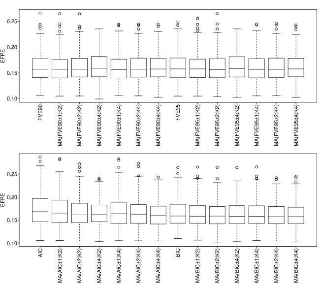
Figure 1: Boxplots of EFPE in simulation design I with $\tau=0.5$. FVE90, FVE with $\gamma=0.90$; FVE95, FVE with $\gamma=0.95$; MA(FVE90$\pm\alpha$, $K\beta$), model averaging method with $\widehat{J}_{n}$ determined by FVE90, with $d=\alpha$, and with weights selected by $\mathrm{CV}_{K=\beta}$; MA(FVE95$\pm\alpha$, $K\beta$), MA(AIC$\pm\alpha$, $K\beta$), and MA(BIC$\pm\alpha$, $K\beta$) have similar definitions.

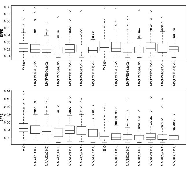
Figure 2: Boxplots of EFPE in simulation design I with $\tau=0.05$. FVE90, FVE with $\gamma=0.90$; FVE95, FVE with $\gamma=0.95$; MA(FVE90$\pm\alpha$, $K\beta$), model averaging method with $\widehat{J}_{n}$ determined by FVE90, with $d=\alpha$, and with weights selected by $\mathrm{CV}_{K=\beta}$; MA(FVE95$\pm\alpha$, $K\beta$), MA(AIC$\pm\alpha$, $K\beta$), and MA(BIC$\pm\alpha$, $K\beta$) have similar definitions.

Next, we compare the proposed model averaging prediction with the other six model averaging and selection methods. We choose $d$-divergence model averaging with $d=4$ coupled with the FVE(0.90) criterion as our model averaging method. We consider $n=100,200,400$ and $\tau=0.5,0.05$, and $K$ is fixed to be 4. In each simulation setting, we normalize the EFPEs of the other six methods by a division of the EFPE of our method. The results are presented in Figure 3. The performance of different methods becomes more similar when $R^{2}$ is large. When $\tau=0.5$, no method clearly denominates the others. Our method is the best in most cases for $n=100,200$. The performances of AIC and BIC seem to be the worst. When $\tau=0.05$, it is clear that our method significantly dominates all the other six methods, and SBIC and FVE(0.90) seem to be the second and third best, respectively when $R^{2}\leq 0.5$. The reason why our method has more advantages than other methods for extreme quantile cases may be that the data at extreme quantiles are usually sparse, the prediction for extreme quantiles is more challenging, and model averaging can address this challenge by using more information from more models. To further show this performance comprehensively, we conduct additional simulation studies with $\tau=0.2$ and $0.1$. The results are displayed in Figure LABEL:fig:normFPE_suppl in the Supplementary Material. From Figures 3 and LABEL:fig:normFPE_suppl, the advantage of model averaging over the other six methods increases as $\tau$ decreases. Overall, the simulation study illustrates the advantage of model averaging over model selection in terms of prediction for extreme quantiles.

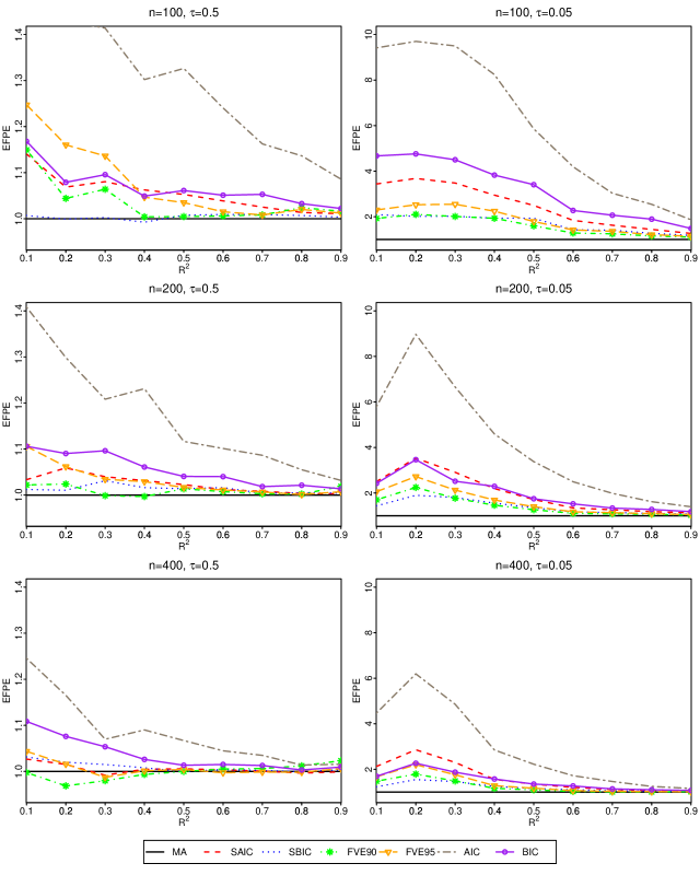
Figure 3: Normalized EFPE in simulation design I for $\tau=0.5$ and $0.05$. MA denotes MA(FVE90$\pm 4$, $K4$).

5.2 Simulation Design II

We consider the same simulation design as that in Subsection 5.1 except for $J_{\max}$, $b^{[1]}(t)$, $a^{[2]}$, and $b^{[2]}(t)$. Specifically, we set $J_{\max}=8$, $b^{[1]}(t)=\sum_{j=1}^{3}j^{-1}\phi_{j}(t)$, $a^{[2]}=2\sum_{j=1}^{3}j^{-1.5}\kappa_{j}^{1/2}$, and $b^{[2]}(t)=\sum_{j=1}^{3}j^{-1.5}\phi_{j}(t)$. The candidate set $\mathcal{J}$ is fixed to be $\{0,1,\ldots,6\}$. Accordingly, the true models are $J^{*}=3,4,5$, or 6, which are included in the candidate models with the candidate set $\mathcal{J}$.

We first evaluate the finite sample performance of the proposed model averaging prediction in the scenario with true candidate models. As in Subsection 5.1, we compare it with the other six model averaging and selection methods by computing the excess final prediction errors. We set $K=4$ and consider $n=100,200,400$ and $\tau=0.5,0.05$. In each simulation setting, we normalize the EFPEs of the other six methods by a division of the EFPE of our method. The results are presented in Figure 4. The performance of different methods becomes more similar when $R^{2}$ is large. When $\tau=0.5$, the performance of our method is the best in some cases (e.g., $R^{2}=0.1,0.4,0.5$) for $n=100$, while our method has no advantage for $n=200,400$. When $\tau=0.05$, our method significantly outperforms the other six methods when $R^{2}\leq 0.6$. To further illustrate the advantage of our method in terms of prediction for extreme quantiles, we conduct additional simulation studies with $\tau=0.2$ and $0.1$. The results are displayed in Figure LABEL:fig:mise_suppl in the Supplementary Material. From Figures 4 and LABEL:fig:mise_suppl, the advantage of our method over the other six methods increases as $\tau$ decreases. This illustrates that even when there is at least one true model in the set of candidate models, our method leads to smaller EFPEs compared with the other six methods for extreme quantiles.

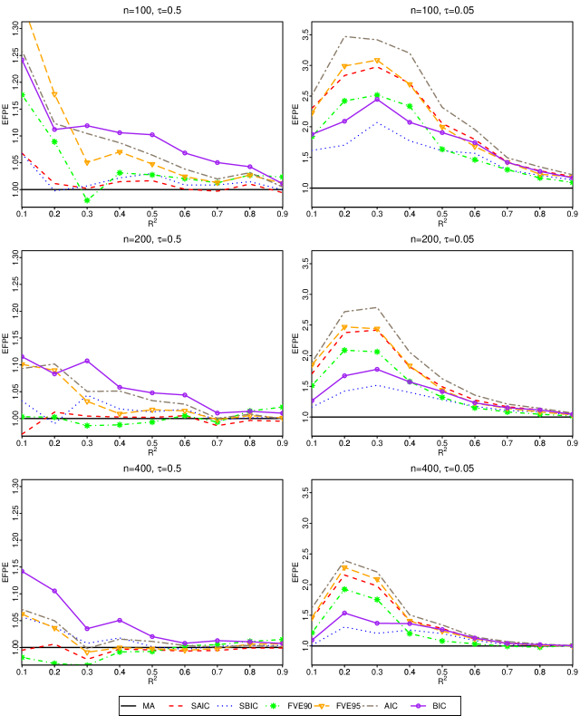
Figure 4: Normalized EFPE in simulation design II for $\tau=0.5$ and $0.05$. MA denotes MA(FVE90$\pm 4$, $K4$).

Next, we verify the consistency of $\widehat{b}_{\widehat{\mathbf{w}}}(t)$ in Theorem 2. We do this by computing the mean integrated squared error (MISE) based on 200 replications. Specifically, the MISE of our estimator is computed as

$$\mathrm{MISE}={1\over 200}\sum_{r=1}^{200}\int_{0}^{1}\left\{\widehat{b}_{\widehat{\mathbf{w}}}(t)^{(r)}-b(t)\right\}^{2}\,dt,$$

where $\widehat{b}_{\widehat{\mathbf{w}}}(t)^{(r)}$ denotes the model averaging estimator of $b(t)$ in the $r$th replication. We set $K=4$ and consider $n=50,100,300,500,700,900,1100$, $R^{2}=0.1,0.5,0.9$, and $\tau=0.5,0.05$. Figure 5 plots MISE against $n$ for each combination of $R^{2}$ and $\tau$. These plots show that as $n$ increases, the MISE of $\widehat{b}_{\widehat{\mathbf{w}}}(t)$ decreases to zero, which reflects the consistency of $\widehat{b}_{\widehat{\mathbf{w}}}(t)$. In addition, we observe that the MISE increases as $R^{2}$ increases. This is not counterintuitive since $\theta$ and $b(t)$ become larger as $R^{2}$ becomes larger. We also compare the performance of $\widehat{b}_{\widehat{\mathbf{w}}}(t)$ with the other six methods, and the results are presented in Section LABEL:sec:simsty of the Supplementary Material for saving space.

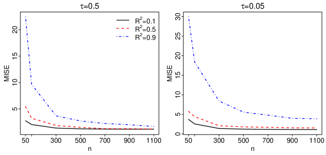
Figure 5: MISE of $\widehat{b}_{\widehat{\mathbf{w}}}(t)$ with $\tau=0.5$ (left) and $\tau=0.05$ (right) under simulation design II.

6 Real Data Analysis

We demonstrate the performance of the proposed model averaging prediction through data on the price of the Bitcoin cryptocurrency. The data set was collected from January 1, 2012 and January 8, 2018 on the exchange platform Bitstamp. We use our method to, based on hourly log-returns of the price of Bitcoin on a given day, predict the $\tau$th quantile of the maximum hourly log-return of Bitcoin price the next day. To reduce the temporal dependence existing in the data, as in Girard et al., (2022), we construct our sample of data by keeping a gap of one day between observations. Specifically, in the $i$th sample $(Y_{i},X_{i})$, the functional covariate $X_{i}$ is the curve of hourly log-returns on day $2i-1$ and the scalar response $Y_{i}$ is the maximum hourly log-return on day $2i$. After deleting missing data, $n=917$ samples are kept in the study. The left panel of Figure 6 provides hourly log-returns of Bitcoin price, and the right panel plots the histogram of maximum hourly log-return of Bitcoin price. Obviously the distribution of maximum hourly log-return is highly right skewed; hence a simple statistic like sample mean cannot adequately describe the (conditional) distribution of $Y_{i}$ given $X_{i}$. We randomly sample 70% of samples as the training data to build the FLQR model and use the remaining 30% of samples as the test data to evaluate the prediction performance. To better assess prediction accuracy, we repeat this $B=200$ times based on random partitions of the data set.

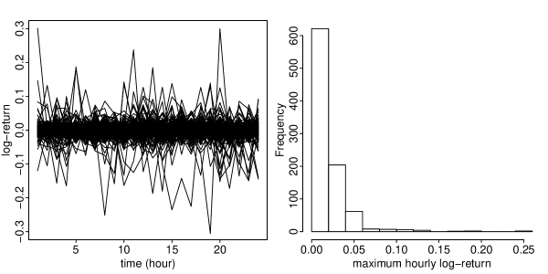
Figure 6: Financial data on the price of Bitcoin. Left: hourly log-returns of Bitcoin price. Right: histogram of the maximum hourly log-return of Bitcoin price.

We consider the $\tau$th quantile prediction with $\tau=0.5$, $0.05$, and $0.01$. To perform prediction using model averaging, we choose the $d$-divergence model averaging described in Subsection 3.3, where $d=0$, 2, 4, 8, 10, 16, 22 and $\widehat{J}_{n}$ is selected by FVE(0.90), FVE(0.95), AIC, and BIC. Table 1 summarizes the averages and standard errors of $\widehat{J}_{n}$, where we can see that BIC selects the smallest number of principal components. We then obtain the optimal weights through the $K$-fold cross-validation, where $K=2$, $4$, and $10$.

Table 1: Results for financial data on the price of Bitcoin. Averages and standard errors (in parentheses) of $\widehat{J}_{n}$ selected by AIC, BIC, FVE(0.90), and FVE(0.95) across the 200 random partitions.

	AIC	BIC	FVE(0.90)	FVE(0.95)
$\tau=0.5$	15.160(5.831)	0.910(1.085)	17.345(0.477)	19.875(0.332)
$\tau=0.05$	14.670(5.360)	2.055(1.911)	17.335(0.473)	19.870(0.337)
$\tau=0.01$	17.545(3.950)	6.820(2.625)	17.290(0.466)	19.865(0.343)

To evaluate each method, we calculate the final prediction error, which are calculated as

$$\mathrm{FPE}(\mathbf{w})={1\over\lfloor 0.3n\rfloor B}\sum_{r=1}^{B}\sum_{i=1}^{\lfloor 0.3n\rfloor}\rho_{\tau}\left(Y_{0,i}^{(r)}-\widehat{Q}_{\tau}(X_{0,i}^{(r)},\mathbf{w})^{(r)}\right),$$

where $\{(Y_{0,i}^{(r)},X_{0,i}^{(r)})\}_{i=1}^{\lfloor 0.3n\rfloor}$ is the test data and $\widehat{Q}_{\tau}(\cdot,\mathbf{w})^{(r)}$ denotes the prediction based on the training data in the $r$th partition. By (3.2), the above FPE also measures the EFPE. Figure 7 illustrates the final prediction errors for $K=2$. For saving space, the all results for $K=2$, $4$, and $10$ are summarized in Figure LABEL:fig:bitcoin_all in the Supplementary Material, which suggest that the performance depends little on $K$. Note that the result of $d=0$ corresponds to that of model selection with $\widehat{J}_{n}$. Table 1 and Figure 7 suggest that for each $\tau$, the FLQR model requires a small number of principal components since the model selected by BIC yields a relatively small prediction error, and the model averaging approaches only slightly reduce it. The results using FVE(0.90), FVE(0.95), and AIC have large prediction errors since they overestimate the numbers of principal components, but these results are much improved when using model averaging with $d=10$ or larger. The data example demonstrates that model averaging improves the prediction performance and can protect against potential prediction loss caused by a single selection criterion.

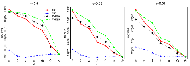
Figure 7: Results for financial data on the price of Bitcoin. Line charts for the $\text{FPEs}\times 100$ with $\tau=0.5$ (left), $\tau=0.05$ (middle), and $\tau=0.01$ (right), where $K=2$.

Finally, we compare our method with the other six model averaging and selection methods described in Section 5. We fix $K=2$ and choose $\mathcal{J}$ in Subsection 3.3 with $d=8$ and $\widehat{J}_{n}$ selected by BIC as the candidate set. The boxplots of FPEs based on the seven methods are displayed in Figure 8. The results demonstrate that our method has the best performance for $\tau=0.05,0.01$. Once again, these outcomes highlight the advantages of our method, especially for extreme quantiles.

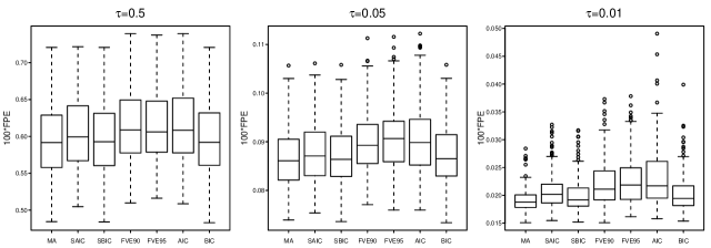
Figure 8: Boxplots of the $\text{FPEs}\times 100$ for financial data on the price of Bitcoin. MA denotes MA(BIC$\pm 8$, $K2$).

7 Discussion

This paper has developed a $K$-fold cross-validation model averaging for the FLQR model. When there is no true model included in the set of candidate models, the weight vector chosen by our method is asymptotically optimal in terms of minimizing the excess final prediction error, whereas when there is at least one true model included, the model averaging parameter estimates are consistent. Our simulations indicate that the proposed method outperforms the other model averaging and selection methods, especially for extreme quantiles. We apply the proposed method to a financial data on the price of Bitcoin.

There are some open questions for future research. First, it is of interest to improve the convergence rate for $\widehat{a}_{\widehat{\mathbf{w}}}$ and $\widehat{b}_{\widehat{\mathbf{w}}}(t)$ in Theorem 2. Second, while we proposed several choices of candidate models and compared their finite sample performances, a theoretical comparison of these choices is still lacking and needs to be done in the future. Another possible research direction is the asymptotic behavior of the selected weights. It is worth noting that Zhang and Liu, (2019) have studied this issue for jackknife model averaging in linear regression, but its application to linear quantile regression remains unknown. Finally, an interesting extension for future studies would be to develop model averaging prediction and estimation for a partial FLQR model (Yao et al.,, 2017).

Supplementary Material

Supplementary material related to this article can be found online. It contains the detailed derivation of the last equality of Equation (3.2), proofs of Theorems 1 and 2, a simulation study continued from Section 5, and additional figures in Sections 5 and 6.

References

- Ando and Li, (2014) Ando, T. and Li, K.-C. (2014). A model-averaging approach for high-dimensional regression. Journal of the American Statistical Association, 109(505):254–265.
- Buckland et al., (1997) Buckland, S. T., Burnham, K. P., and Augustin, N. H. (1997). Model selection: An integral part of inference. Biometrics, 53(2):603–618.
- Cai and Hall, (2006) Cai, T. T. and Hall, P. (2006). Prediction in functional linear regression. The Annals of Statistics, 34(5):2159–2179.
- Cardot et al., (2005) Cardot, H., Crambes, C., and Sarda, P. (2005). Quantile regression when the covariates are functions. Journal of Nonparametric Statistics, 17(7):841–856.
- Chen and Müller, (2012) Chen, K. and Müller, H.-G. (2012). Conditional quantile analysis when covariates are functions, with application to growth data. Journal of the Royal Statistical Society: Series B, 74(1):67–89.
- Cheng and Hansen, (2015) Cheng, X. and Hansen, B. E. (2015). Forecasting with factor-augmented regression: A frequentist model averaging approach. Journal of Econometrics, 186(2):280–293.
- Cuevas, (2014) Cuevas, A. (2014). A partial overview of the theory of statistics with functional data. Journal of Statistical Planning and Inference, 147:1–23.
- Ferraty et al., (2005) Ferraty, F., Rabhi, A., and Vieu, P. (2005). Conditional quantiles for dependent functional data with application to the climatic El Niño phenomenon. Sankhyā, 67(2):378–398.
- Ferraty and Vieu, (2006) Ferraty, F. and Vieu, P. (2006). Nonparametric Functional Data Analysis: Theory and Practice. Springer, New York.
- Gao et al., (2016) Gao, Y., Zhang, X., Wang, S., and Zou, G. (2016). Model averaging based on leave-subject-out cross-validation. Journal of Econometrics, 192(1):139–151.
- Giessing and He, (2019) Giessing, A. and He, X. (2019). On the predictive risk in misspecified quantile regression. Journal of Econometrics, 213(1):235–260.
- Girard et al., (2022) Girard, S., Stupfler, G., and Usseglio-Carleve, A. (2022). Functional estimation of extreme conditional expectiles. Econometrics and Statistics, 21:131–158.
- Hansen and Racine, (2012) Hansen, B. E. and Racine, J. S. (2012). Jackknife model averaging. Journal of Econometrics, 167(1):38–46.
- Horváth and Kokoszka, (2012) Horváth, L. and Kokoszka, P. (2012). Inference for Functional Data with Applications. Springer, New York.
- Hsing and Eubank, (2015) Hsing, T. and Eubank, R. L. (2015). Theoretical Foundations of Functional Data Analysis, with an Introduction to Linear Operators. Wiley, Chichester.
- Kato, (2012) Kato, K. (2012). Estimation in functional linear quantile regression. The Annals of Statistics, 40(6):3108–3136.
- Knight, (1998) Knight, K. (1998). Limiting distributions for regression estimators under general conditions. The Annals of Statistics, 26(2):755–770.
- Koenker, (2005) Koenker, R. (2005). Quantile Regression. Cambridge University Press, Cambridge.
- Koenker and Bassett, (1978) Koenker, R. and Bassett, G. (1978). Regression quantiles. Econometrica, 46(1):33–50.
- Li et al., (2022) Li, M., Wang, K., Maity, A., and Staicu, A.-M. (2022). Inference in functional linear quantile regression. Journal of Multivariate Analysis, 190:104985.
- Li and Hsing, (2010) Li, Y. and Hsing, T. (2010). Uniform convergence rates for nonparametric regression and principal component analysis in functional/longitudinal data. The Annals of Statistics, 38(6):3321–3351.
- Li et al., (2010) Li, Y., Wang, N., and Carroll, R. J. (2010). Generalized functional linear models with semiparametric single-index interactions. Journal of the American Statistical Association, 105(490):621–633.
- Li et al., (2013) Li, Y., Wang, N., and Carroll, R. J. (2013). Selecting the number of principal components in functional data. Journal of the American Statistical Association, 108(504):1284–1294.
- Liu, (2015) Liu, C.-A. (2015). Distribution theory of the least squares averaging estimator. Journal of Econometrics, 186(1):142–159.
- Liu and Okui, (2013) Liu, Q. and Okui, R. (2013). Heteroscedasticity-robust model averaging. The Econometrics Journal, 16(3):463–472.
- Lu and Su, (2015) Lu, X. and Su, L. (2015). Jackknife model averaging for quantile regressions. Journal of Econometrics, 188(1):40–58.
- Ma et al., (2019) Ma, H., Li, T., Zhu, H., and Zhu, Z. (2019). Quantile regression for functional partially linear model in ultra-high dimensions. Computational Statistics & Data Analysis, 129:135–147.
- Magnus et al., (2010) Magnus, J. R., Powell, O., and Prüfer, P. (2010). A comparison of two model averaging techniques with an application to growth empirics. Journal of Econometrics, 154(2):139–153.
- Morris, (2015) Morris, J. S. (2015). Functional regression. Annual Review of Statistics and Its Application, 2:321–359.
- Müller and Stadtmüller, (2005) Müller, H.-G. and Stadtmüller, U. (2005). Generalized functional linear models. The Annals of Statistics, 33(2):774–805.
- Peng and Yang, (2022) Peng, J. and Yang, Y. (2022). On improvability of model selection by model averaging. Journal of Econometrics, 229(2):246–262.
- Ramsay and Silverman, (2005) Ramsay, J. O. and Silverman, B. W. (2005). Functional Data Analysis. Springer, New York, 2nd edition.
- Sang et al., (2022) Sang, P., Shang, Z., and Du, P. (2022). Statistical inference for functional linear quantile regression. arXiv preprint arXiv:2202.11747.
- Wang et al., (2016) Wang, J.-L., Chiou, J.-M., and Müller, H.-G. (2016). Functional data analysis. Annual Review of Statistics and Its Application, 3:257–295.
- Wang et al., (2023) Wang, M., Zhang, X., Wan, A. T., You, K., and Zou, G. (2023). Jackknife model averaging for high-dimensional quantile regression. Biometrics, 79(1):178–189.
- (36) Yao, F., Müller, H.-G., and Wang, J.-L. (2005a). Functional data analysis for sparse longitudinal data. Journal of the American Statistical Association, 100(470):577–590.
- (37) Yao, F., Müller, H.-G., and Wang, J.-L. (2005b). Functional linear regression analysis for longitudinal data. The Annals of Statistics, 33(6):2873–2903.
- Yao et al., (2017) Yao, F., Sue-Chee, S., and Fan, W. (2017). Regularized partially functional quantile regression. Journal of Multivariate Analysis, 156:39–56.
- Yuan and Yang, (2005) Yuan, Z. and Yang, Y. (2005). Combining linear regression models: When and how? Journal of the American Statistical Association, 100(472):1202–1214.
- Zhang and Zou, (2020) Zhang, H. and Zou, G. (2020). Cross-validation model averaging for generalized functional linear model. Econometrics, 8(1):7.
- Zhang, (2013) Zhang, J.-T. (2013). Analysis of Variance for Functional Data. Chapman & Hall, London.
- Zhang et al., (2018) Zhang, X., Chiou, J.-M., and Ma, Y. (2018). Functional prediction through averaging estimated functional linear regression models. Biometrika, 105(4):945–962.
- Zhang and Liu, (2019) Zhang, X. and Liu, C.-A. (2019). Inference after model averaging in linear regression models. Econometric Theory, 35(4):816–841.
- Zhang et al., (2013) Zhang, X., Wan, A. T., and Zou, G. (2013). Model averaging by jackknife criterion in models with dependent data. Journal of Econometrics, 174(2):82–94.
- Zhang and Wang, (2016) Zhang, X. and Wang, J.-L. (2016). From sparse to dense functional data and beyond. The Annals of Statistics, 44(5):2281–2321.