Quantifying the information lost in optimal covariance matrix cleaning

Abstract

In this work, we examine the prevalent use of Frobenius error minimization in covariance matrix cleaning. Currently, minimizing the Frobenius error offers a limited interpretation within information theory. To better understand this relationship, we focus on the Kullback-Leibler divergence as a measure of the information lost by the optimal estimators. Our analysis centers on rotationally invariant estimators for data following an inverse Wishart population covariance matrix, and we derive an analytical expression for their Kullback-Leibler divergence. Due to the intricate nature of the calculations, we use genetic programming regressors paired with human intuition. Ultimately, we establish a more defined link between the Frobenius error and information theory, showing that the former corresponds to a first-order expansion term of the Kullback-Leibler divergence.

Keywords Random Matrix Theory  $\cdot$ Covariance Matrix Estimation $\cdot$ Genetic Regressor Programming  $\cdot$ High-Dimension Statistics  $\cdot$ Information theory

1 Introduction

Dependence characterization in multivariate statistics heavily relies on covariance matrix estimation, which accordingly is a tool of great importance in many areas such as physics [1], neuroscience [2], and finance [3]. However, the sample covariance is remarkably noisy when the number of features is of the same order as the number of data points [4]. This situation is a frequent issue in many applications. For example, data on neural brain connections contains a large number of connections (features) but has small sample sizes [2, 5]. In finance, constructing a well-diversified portfolio requires many assets (features). In contrast, rapid shifts in financial market dependencies can only be captured by short calibration windows [6, 7]. These are just a select few examples, with many other fields also confronting this issue.

Numerous techniques have been developed to improve the estimation of noisy covariance matrices. Eigenvalue clipping [3] and linear shrinkage [7, 8] laid the groundwork in this area. Building upon these early works, a major improvement was the introduction of nonlinear shrinkage (NLS), initially proposed by Ledoit and Péché [9], and further expanded by Ledoit and Wolf [10, 11]. These methods, which are extensively reviewed in [12, 13], primarily originate from or can be understood within the framework of random matrix theory. Machine learning techniques have also been explored for enhancing covariance matrix estimation. Techniques such as validation or cross-validation offer numerical solutions to the NLS problem for enhancing the estimator performances [14, 15]. Alongside, orthogonal approaches like hierarchical clustering [16] and boosting methods [17] have independently emerged as effective methods in this domain. Generally speaking, applying constraints stabilizes the estimated covariance matrix, reducing its noise [12]. Notable examples include methods based on factor models [18, 19, 20] and Bayesian estimation. The latter uses priors to effectively model the population covariance matrix [21, 22].

All these methods aim to reduce the noise in estimated covariance matrices. Yet, questions often arise about what these methods actually optimize and, more crucially, what they ideally should optimize. While the latter question is problem-specific, a make-do with good enough methods often prevails. For example, to minimize the variance of a portfolio, computations on the inverse covariance matrix are necessary. Nonetheless, employing NLS [9] on the covariance matrix itself is deemed acceptable as it minimizes the square distance between the filtered and the true matrix, i.e., the Frobenious error on the covariance matrix. Expectantly, in a realistic context characterized by finite sample size and time variability, minimizing the Frobenious error is not equivalent to minimizing the variance of a portfolio [23]. Despite this, working with the Frobenious error is sometimes the only way to obtain analytical results.

More generally speaking, the Frobenius error lacks a clear interpretation when approaching the problem from an information theory perspective. Instead, the Kullback-Leibler (KL) divergence quantifies, by definition, the information lost when approximating the true distribution with an inferred one. The use of the KL divergence as a performance metric for evaluating filtered covariance matrix estimators was initially investigated in Ref. [24, 25, 26]. They highlighted that the expected KL divergence is independent of the population (true) eigenvectors when the data is generated using Gaussian multivariate noise [25]. This unique attribute, alongside its capacity to measure information loss, earmarks the KL divergence as a valuable tool, especially in complex scenarios where eigenvectors are non-trivial. Despite its benefits, the application of KL divergence is limited in existing literature, probably because of its analytical challenges.

We achieved further progress in applying information theory to covariance matrix cleaning. Specifically, we analytically measured the KL divergence of optimal estimators. Given the ambiguity surrounding the “optimal” estimator, our investigation narrows its focus to the Rotationally Invariant Estimators (RIE) class. These estimators modify the eigenvalues of sample covariance matrices while maintaining the sample eigenvectors. In this simple setting, an optimal RIE is known as the Oracle estimator if it minimizes the Frobenius error. Interestingly, the Oracle estimator also minimizes the KL divergence for infinite sample sizes [27] as both cost functions have the same minimum. However, with a realistic finite sample size, opting to minimize the Frobenius norm over the KL divergence results in notable discrepancies.

To simplify our estimation problem, which involves computing the KL for the Oracle estimator, we focus on data distributed according to the inverse Wishart distribution. This serves as a starting point, and while it offers some analytical accessibility, it is by no means a limitation. The inverse Wishart distribution is one of the few for which analytic results are relatively easy to obtain. For example, the optimal RIE estimator is the linear shrinkage [28]. Despite its simplicity, this distribution can approximate the eigenvalue distributions observed in real-world applications [28, 29]. Nevertheless, deriving the analytical expression of the KL divergence remains a challenge. As a shortcut, we employ Genetic Programming Regressors (GPR), a machine learning tool adept at solving symbolic regression problems [30, 31]. Operating through a tree representation of equations, it uses crossover and mutation operators to evolve potential solution populations based on Darwinian selection principles. After analyzing the GPR results, we employed human intuition to identify an incomplete series expansion within its output. Recognizing this allowed us to extend this partial sum to an infinite one, successfully obtaining the complete formula for the KL divergence of the optimal RIE in the inverse Wishart case.

The paper is organized as follows: in Section 2, we set the definitions; in Section 3, we derive analytically the KL divergence for sample covariance matrices; in Section 4, we apply GPR to compute the KL divergence to the more complex case of the filtered covariance matrix, and finally, in Section 5, we link the KL divergence to the Frobenius error.

2 Definitions

2.1 Kullback-Leibler Divergence

The KL divergence, also known as relative entropy, measures how one probability distribution diverges from a second, expected probability distribution. Given probability measures $P$ and $Q$ over a set $\mathcal{X}$, the KL divergence is formally defined as:

$$\textrm{KL}(P||Q):=\int_{\mathcal{X}}\left(\log\frac{P}{Q}\right)dP=\mathcal{E}\left[\log\left(\frac{P(x;{\bf C})}{Q(x;{\bf S})}\right)\right]_{P(x;{\bf C})}.$$ (1)

Conceptually, the KL divergence quantifies the “distance” between the two probability measures $P$ and $Q$. However, it is important to note that the KL divergence is not a true distance metric as it is not symmetric, as $\textrm{KL}(P||Q)\neq\textrm{KL}(Q||P)$ in general.

In this context, the KL divergence represents the average logarithmic difference between the probabilities $P$ and $Q$, where the average is taken using the probabilities $P$. Consequently, it provides an estimate of the expected amount of information (in bits, for logarithm base 2, or nats, for natural logarithm) lost when $Q$ is used to approximate $P$.

In the case of multivariate normal variables with true population covariance $\bm{C}$ and estimator $\bm{S}$, the KL divergence simplifies to

$$\textrm{KL}(\bm{C}||\bm{S})=\frac{1}{2}\left(\textrm{Tr}\left(\bm{S}^{-1}\bm{C}\right)+\log\left(\frac{\det(\bm{S})}{\det(\bm{C})}\right)-n\right).$$ (2)

This work focuses on a normalized version of the KL divergence. By dividing the KL divergence by the dimension of the covariance matrix $n$, we obtain a scaled measure of the divergence, which is particularly useful for high-dimensional problems:

$$\overline{\textrm{KL}}(\bm{C}||\bm{S})=\frac{\textrm{KL}(\bm{C}||\bm{S})}{n}.$$ (3)

This normalized KL divergence provides a more interpretable measure of the information loss per dimension when the estimator $\bm{S}$ is used to approximate the true population covariance $\bm{C}$.

2.2 Populations, Samples, and Oracle Estimator

Let $n\in\mathbb{N}^{*}$ and $p>0$. Let us define $q^{*}=\frac{p}{1+p}$ and $t^{*}=\lfloor\frac{n}{q^{*}}\rfloor$. Let us consider $(\bm{m}_{i})_{1\leq i\leq t^{*}}$ iid vectors of $\mathbb{R}^{n}$ such that $\bm{m}_{1}\sim\mathcal{N}(0,\bm{\Sigma})$. Since we focus on the white case, $\bm{\Sigma}=\bm{\mathds{1}}$. We then define $\bm{M}=(\bm{m}_{1},...,\bm{m}_{t^{*}})\in\mathbb{R}^{n\times t^{*}}$. Then

$$\bm{W}_{q^{*}}=\frac{1}{t^{*}}\bm{MM}^{\dagger}$$ (4)

the following matrix is Wishart $(n,q^{*})$ and

$$\bm{\mathcal{W}}^{-1}_{np}=(1-q^{*})\bm{W}^{-1}$$ (5)

is an Inverse Wishart $(n,p)$. The constant of $(1-q^{*})$ is added so that the expected value of the normalized trace of an Inverse Wishart is equal to $1$.

The Inverse Wishart distribution displays a spread-out distribution of the eigenvalues when $p>0$ and becomes marked when $p$ is very large (and therefore $q^{*}$ approaches one); such behavior cannot be achieved with a simpler Wishart matrix. In addition, the eigenvectors of a white Wishart matrix are distributed according to the Haar measure on the orthogonal group [32].

The associated data matrix $\bm{X}$, of dimensions $n\times t$, is generated from a centered multivariate normal distribution with population covariance matrix $\bm{C}:=\bm{\mathcal{W}}^{-1}_{np}$. Following this, after removing the average of each column of $\bm{X}$, the sample covariance matrix is defined as

$$\bm{E}=\frac{1}{t}\bm{XX}^{\dagger},$$ (6)

with $q:=\frac{n}{t}$ the ratio between the size of the matrix and the number of observations.

This sample covariance matrix $\bm{E}$ is decomposed spectrally as

$$\bm{E}=\bm{V\Lambda V}^{\dagger},$$ (7)

where $\bm{V}$ is the matrix of eigenvectors and $\bm{\Lambda}$ is the diagonal matrix of eigenvalues. From this spectral decomposition, we can extract the Oracle eigenvalues as

$$\bm{\Lambda}_{O}=\textrm{diag}\left(\bm{V}^{\dagger}\bm{CV}\right),$$ (8)

where the operator $\textrm{diag}(\bullet)$ nullifies the off-diagonal elements of the matrix.

With the Oracle eigenvalues $\bm{\Lambda}_{O}$ in hand, we define the Oracle estimator $\bm{\Xi}(\bm{\Lambda}_{O})$ as

$$\bm{\Xi}(\bm{\Lambda}_{O}):=\bm{V\Lambda}_{O}\bm{V}^{\dagger}.$$ (9)

This Oracle estimator represents an idealized estimator that is aware of the true population covariance. $\bm{\Xi}(\bm{\Lambda}_{O})$ is the Rotational Invariant Estimator (RIE) that minimizes the Frobenius norm distance with the population matrix $\bm{C}$ [9, 28, 27].

Furthermore, in the case of multivariate normal or infinite multivariate t-students variables, it has been proved [27] that $\bm{\Xi}(\bm{\Lambda}_{O})$ is also the RIE that minimizes the KL divergence $\textrm{KL}(\bm{C}||\bm{\Xi}(\bm{\Lambda}))$. This finding implies that the Oracle estimator, derived from the inverse Wishart population covariance matrix is, in some idealized context, optimal for minimizing both the Frobenius norm and the KL divergence. Therefore, it is the proper tool for covariance matrix estimation in high-dimensional settings.

3 Quantifying Information Loss for Sample Covariances

In this section, we quantify analytically the expected loss of information when the population matrix $\bm{C}$ is approximated by the sample estimator $\bm{E}$.

For the sake of generality, we consider $\bm{C}\in\mathbb{R}^{n\times n}$ a generic positive defined population covariance matrix, i.e., not necessarily a white inverse Wishart, and $\bm{E}$, the sample covariance, obtained from $\bm{X}\in\mathbb{R}^{n\times t}$ with $t>n$ multinomial variables with population matrix $\bf C$.

In the limit of large $n$, this expected information loss, as measured by the normalized KL divergence, is given by

$$\mathcal{\bm{E}}[\overline{\textrm{KL}}(\bm{C}||\bm{E})]=\frac{1-q}{2q}\log\left(\frac{1}{1-q}\right)+\frac{1}{2(1-q)}-1.$$ (10)

Let us briefly explain where this equation comes from. Firstly, the normalized KL is defined as

$$\mathcal{E}[\overline{\textrm{KL}}(\bm{C}||\bm{E})]=\frac{1}{2}\mathcal{E}\left[\tau(\bm{E^{-1}C})-1+\frac{1}{n}\log\left(\frac{\det(\bm{E})}{\det(\bm{C})}\right)\right]$$ (11)

where $\tau(\bullet)=\frac{1}{n}Tr(\bullet)$ is the normalized trace.

By noticing that $\bm{E}=\sqrt{\bm{C}}\bm{W}_{q}\sqrt{\bm{C}}$ where $\bm{W}_{q}$ is a white Wishart generated by $t=\lfloor\frac{n}{q}\rfloor$ observations, which is independent of $\bm{C}$, our expression simplifies to

$$\mathcal{E}[\overline{\textrm{KL}}(\bm{C}||\bm{E})]=\frac{1}{2}\mathcal{E}\left[\tau(\bm{W}_{q}^{-1})-1+\frac{1}{n}\log(\det(\bm{W}_{q}))\right].$$ (12)

We can already notice that the KL does not depend on the choice of the population matrix when the observations are generated by a Gaussian multiplicative distribution.

The first term is known [28]:

$$\mathcal{E}[\tau(\bm{W}_{q}^{-1})]=\frac{1}{1-q}.$$ (13)

To compute the second term, we can use the fact that the spectral density of a white Wishart follows for Marčenko-Pastur in the asymptotic limit ($n,t\rightarrow\infty$ with $\frac{n}{t}\rightarrow q$) and were able to compute it using Mathematica [33], which yields

$$\mathcal{E}\left[\frac{1}{n}\log(\det(\bm{W}_{q}))\right]=\frac{1-q}{q}\log\left(\frac{1}{1-q}\right)-1.$$ (14)

The above equation provides a measure of how much information, on average, is lost when the population covariance matrix $\bm{C}$ is approximated by the sample covariance matrix $\bm{E}$.

Furthermore, suppose we are interested in comparing the loss of information between two matrices, $\bm{E}_{\textrm{in}}$ and $\bm{E}_{\textrm{out}}$, both derived from the same population covariance $\bm{C}$ but with different parameters $q_{\textrm{in}}$ and $q_{\textrm{out}}$. The corresponding loss of information is given by

$$\mathcal{E}[\overline{\textrm{KL}}(\bm{E}_{\textrm{out}}||\bm{E}_{\textrm{in}})]=\frac{1-q_{\textrm{in}}}{2q_{\textrm{in}}}\log\left(\frac{1}{1-q_{\textrm{in}}}\right)-\frac{1-q_{\textrm{out}}}{2q_{\textrm{out}}}\log\left(\frac{1}{1-q_{\textrm{out}}}\right)+\frac{1}{2(1-q_{\textrm{in}})}-\frac{1}{2}.$$ (15)

This equation provides a means of assessing the relative loss of information when using different sample covariance matrices to approximate the same population covariance matrix.

It is a consequence of Eq. (10), let us briefly explain why

$$\mathcal{E}[\overline{\textrm{KL}}(\bm{E}_{\textrm{out}}||\bm{E}_{\textrm{in}})] =\frac{1}{2}\mathcal{E}\left[\tau(\bm{W}^{-1}_{\textrm{in}}\bm{W}_{\textrm{out}})-1+\frac{1}{n}\log\left(\frac{\det(\bm{E}_{\textrm{out}})}{\det(\bm{E}_{\textrm{in}})}\right)\right]$$ (16)

$$=\frac{1}{2}\mathcal{E}\left[\tau(\bm{E}^{-1}_{\textrm{in}}\bm{E}_{\textrm{out}})-1+\frac{1}{n}\log\left(\det(\bm{W}_{\textrm{in}}\right)-\frac{1}{n}\log(\det(\bm{W}_{\textrm{out}}))\right].$$ (17)

Using the fact that the white Wisharts $\bm{W}_{\textrm{in}}$ and $\bm{W}_{\textrm{out}}$ are asymptotically free in the large limit and the moments of the log Marcenko-Pastur distribution, we obtain

$$\mathcal{E}[\overline{\textrm{KL}}(\bm{E}_{\textrm{out}}||\bm{E}_{\textrm{in}})] =\frac{1}{2}\left(\frac{1}{1-q_{\textrm{in}}}-1+\frac{1-q_{\textrm{in}}}{q_{\textrm{in}}}\log\left(\frac{1}{1-q_{\textrm{out}}}\right)-1-\frac{1-q_{\textrm{out}}}{q_{\textrm{out}}}\log\left(\frac{1}{1-q_{\textrm{out}}}\right)+1\right)$$ (18)

$$=\frac{1}{2(1-q_{\textrm{in}})}+\frac{1-q_{\textrm{in}}}{2q_{\textrm{in}}}\log\left(\frac{1}{1-q_{\textrm{out}}}\right)-\frac{1-q_{\textrm{out}}}{2q_{\textrm{out}}}\log\left(\frac{1}{1-q_{\textrm{out}}}\right)-\frac{1}{2}$$ (19)

While the expected KL divergence in the finite sample size regime is also known [25], it involves sums over digamma functions, which are not conducive for analytical computations.

It is worth noting that these results are applicable to any population covariance matrix and, thus, not restricted to the Wishart distribution. This broad applicability renders our findings useful in a wide range of practical scenarios beyond the scope of this work.

4 Kullback-Leibler Divergence for the Oracle of an Inverse Wishart

4.1 Inherent Mathematical Challenges for Analytical Derivation

The process of optimally deriving the KL divergence of a RIE that converges to the Oracle for an inverse Wishart matrix presents a variety of mathematical challenges [28].

For the white inverse Wishart prior, it is known that the optimal RIE corresponds to a linear shrinkage of the sample covariance [28] and is given by

$$\bm{\Xi}(\bm{\Lambda}_{O})=r(\bm{E}-\bm{\mathds{1}})+\bm{\mathds{1}},$$ (20)

where

$$r=\frac{np}{n(p+q)-pq}.$$ (21)

Subsequently, the KL divergence related to this estimator is given by

$$\textrm{KL}(\bm{C}||\bm{\Xi}(\bm{\Lambda}_{O}))=\frac{1}{2}\left(\textrm{Tr}\left(\bm{\Xi}^{-1}(\bm{\Lambda}_{O})C\right)+\sum_{i=1}^{n}\left(\log\Lambda^{O}_{i}-\log\zeta_{i}\right)-n\right).$$ (22)

Here, $\zeta_{i}$ denotes the eigenvalues of the population matrix. The determination of the expected value in the above equation requires multiple approximations. For instance, obtaining the expected value of the logarithm necessitates a Taylor expansion due to the nonlinearity of the logarithmic function. Furthermore, the calculation of the trace correlation needs intricate knowledge of the interdependence among the eigenvalues of the sample estimator.

These mathematical complexities underline the inherent challenge in obtaining an analytical solution for the KL divergence in the case of the Oracle of a white inverse Wishart. In essence, the interplay of nonlinearities, random variables, and dependencies presents considerable obstacles to the derivation of an analytical solution. Therefore, we seek a novel approach to tackle this problem, which we explore in the following sections.

4.2 Symbolic Machine Learning

In order to derive the expected value of the normalized KL divergence for an arbitrary white inverse Wishart matrix $\bm{\mathcal{W}}^{-1}_{np}$ in the large $n$ regime, we implemented a symbolic machine learning approach. This involved sampling $5,000$ Wishart matrices with randomly chosen parameters $q^{*}\in(0,1)$ and $n=1,000$, and subsequently extracting sample covariances $\bm{E}$ from these matrices with random $q\in(0,1)$. For each pair of matrices, we computed the Oracle estimator $\bm{\Xi}(\bm{\Lambda}_{O})$.

Our approach relied on a genetic symbolic regressor [34]. We initiated the process with a population of $50,000$ potential solutions, set the parsimony coefficient to $10^{-4}$, and allowed for $40$ generation rounds. All other parameters were left at their default settings. A preliminary analysis of the simulation data suggested that we should use the parameters $q$ and $r$ (as defined in Eq. (21)) as input for the regressor, with the goal of minimizing the mean square error of the simulated normalized KL divergence obtained from Eqs. (2) and (3).

Because of the tendency of genetic algorithms to become entrapped in local minima if not adequately tuned, we ran a total of four independent rounds. From these, we identified a generic term for the normalized KL divergence

$$\mathcal{E}[\overline{\textrm{KL}}(\bm{\mathcal{W}}^{-1}_{np}||\bm{\Xi}(\bm{\Lambda}_{O}))]\approx\frac{1}{4}rq-\left(\frac{1}{4}\ rq\right)^{2}.$$ (23)

This equation bears a resemblance to a second-order Taylor expansion. Considering the large $n$ limit of

$$\lim_{n\to\infty}rq=\frac{q^{*}q}{q^{*}+q-q^{*}q}.$$ (24)

Eq. (23) can be transformed into

$$\mathcal{E}[\overline{\textrm{KL}}(\bm{\mathcal{W}}^{-1}_{np}||\bm{\Xi}(\bm{\Lambda}_{O}))]\approx\frac{1}{4}\frac{q^{*}q}{q^{*}+q-q^{*}q}-\left(\frac{1}{4}\frac{q^{*}q}{q^{*}+q-q^{*}q}\right)^{2}.$$ (25)

To validate our assumption, we performed a second round of tests, this time expanding the range of $q^{*}\in(0,1)$ and $q\in(0,7)$. It’s important to note that when $q>1$, the sample matrix $E$ will be singular, but not the Oracle $\bm{\Xi}(\bm{\Lambda}_{O})$. Our analysis of this new data set revealed a discrepancy regarding the prediction of (25).

We attempted to expand Eq. (25) into a suitable progression:

$$\mathcal{E}[\overline{\textrm{KL}}(\bm{\mathcal{W}}^{-1}_{np}||\bm{\Xi}(\bm{\Lambda}_{O}))]=\sum_{k=1}^{\infty}(-1)^{k-1}\left(\frac{1}{4}\frac{q^{*}q}{q^{*}+q-q^{*}q}\right)^{k},$$ (26)

which yielded an exceptional match with the predictions as the approximation order increased, as depicted in Fig. 1.

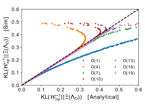
Figure 1: Comparison of the convergence of the series for different orders of approximation of Eq. (26) with parameters $n=1000$, $q^{*}\in(0,1)$ and $q\in(0,7)$.

Moreover, it is here possible to recognize the Taylor-expansion of the function $x\rightarrow\frac{1}{1+x}$

$$\mathcal{E}[\overline{\textrm{KL}}(\bm{\mathcal{W}}^{-1}_{np}||\bm{\Xi}(\bm{\Lambda}_{O}))]=\frac{1}{4}rq\sum_{k=0}^{\infty}(-1)^{k}\left(\frac{1}{4}rq\right)^{k}=\frac{1}{4}rq\frac{1}{1+\frac{1}{4}rq}.$$ (27)

Finally, by replacing $r$ by its value in the high dimension limit, we obtain

$$\mathcal{E}[\overline{\textrm{KL}}(\bm{\mathcal{W}}^{-1}_{np}||\bm{\Xi}(\bm{\Lambda}_{O}))]=\frac{pq}{4p+4q+pq},$$ (28)

which converges if and only if

$$rq=\frac{q^{*}q}{q^{*}+q-q^{*}q}<4.$$ (29)

Let us remind that the shrinkage coefficient $r$ necessarily lies in $[0,1]$ interval; therefore, the divergence can only occur when $q>4$, which means that the number of features should be at least $4$ times larger than the number of observations.

The left panel of Fig. 2 shows strong agreement with Eq. (25). The right panel of Fig. 2 showcases the convergence region defined by Eq. (29), with two asymptotic values $q^{*}=0.8$ and $q=4$.

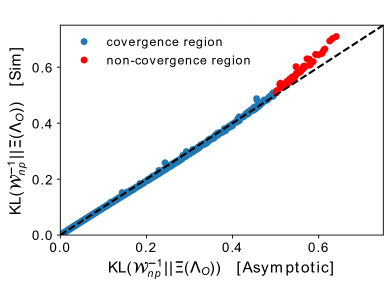
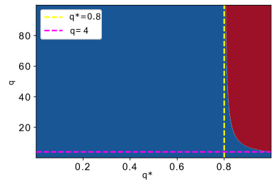
Figure 2: The left panel shows the agreement of the asymptotic equation (25) for parameters $n=1000$, $q^{*}\in(0,1)$ and $q\in(0,7)$; the right panel shows the convergence region of (29); in the red region, the inequality is not respected.

5 Analysis of the Frobenius Error

In the preceding sections, we have extensively analyzed the KL divergence in the context of the optimal linear shrinkage estimator. However, a substantial part of the existing literature focuses on the Frobenius error, another important metric for the evaluation of the performance of estimators. While both the KL divergence and Frobenius error are key in measuring the discrepancies between the estimated and true covariance matrices, they provide different perspectives and may lead to varying conclusions. Therefore, in order to ensure a comprehensive understanding of the linear shrinkage estimator, it is crucial to scrutinize its performance in terms of the Frobenius error as well.

Notably, we show that in the case of the white inverse Wishart distribution, a direct relationship exists between the KL divergence and the Frobenius error, thereby providing a unifying perspective that bridges these two important measures. This analysis will facilitate the comparison of our results with those of previous studies that predominantly focus on the Frobenius error, broadening the overall understanding of the linear shrinkage estimator in the process.

Given our population matrix $\bm{C}$ and the established assumption that it follows a white inverse Wishart distribution with parameter $p$, we can write the Frobenius Error of the Oracle as

$$\overline{\textrm{Frob}}((\bm{C}||\bm{\Xi}(\bm{\Lambda}_{O}))=\tau((\bm{\Xi}(\bm{\Lambda}_{O})-\bm{C})^{2})\hskip 8.53581pt\mbox{where}\hskip 2.84526pt\tau\hskip 2.84526pt\mbox{is the notmalized trace.}$$ (30)

This follows directly from the definition of the Frobenius norm and the fact that the optimal linear shrinkage is equal to the Oracle when estimating a population matrix using the sample covariance $\bm{E}$. Also, it is known that the expected value of the Frobenius error of estimation of a white inverse Wishart is the following [28, 35]

$$\mathcal{E}[\overline{\textrm{Frob}}((\bm{C}||\bm{\Xi}(\bm{\Lambda}_{O}))]=(1-r)^{2}p+qr^{2}.$$ (31)

Given that $r=\frac{p}{p+q}$ in the large limit, we finally obtain

$$\mathcal{E}[\overline{\textrm{Frob}}((\bm{C}||\bm{\Xi}(\bm{\Lambda}_{O}))]=\frac{pq}{p+q}.$$ (32)

Importantly, we note that if $p$ or $q$ are small,

$$\mathcal{E}[\overline{\textrm{KL}}(\bm{C}||\bm{\Xi}(\bm{\Lambda}_{O}))]\sim\frac{1}{4}\mathcal{E}[\overline{\textrm{Frob}}((\bm{C}||\bm{\Xi}(\bm{\Lambda}_{O})))].$$ (33)

This shows a clear relationship between the Frobenius error and the KL divergence in the case of a white inverse Wishart population matrix, a key point in our analysis. From the Taylor-Expansion of the KL divergence (eq. (23)), we can understand where the $\frac{1}{4}$ factor term comes from, as we notice that the first-order term of the expected KL, $\frac{1}{4}rq$, coincides exactly with $\frac{1}{4}$ of the expected Frobenius error

$$\mathcal{E}[\overline{\textrm{KL}}(\bm{\mathcal{W}}^{-1}_{np}||\bm{\Xi}(\bm{\Lambda}_{O}))]=\sum_{k=1}^{\infty}(-1)^{k-1}\left(\frac{1}{4}rq\right)^{k}=\sum_{k=1}^{\infty}(-1)^{k-1}\left(\frac{1}{4}\mathcal{E}[\overline{\textrm{Frob}}(\bm{C}||\bm{\Xi}(\bm{\Lambda}_{O})])\right)^{k}.$$ (34)

As a consequence, in the case of a white inverse Wishart population matrix, the expected Frobenius error of estimation is proportional to the first-order approximation of the KL divergence. We point out that while the Frobenius error is always finite, the KL divergence can be infinite at the same time. Therefore it helps detect when all the information is lost by the estimation.

6 Conclusions

In this work, we presented a novel method for computing the analytical expected value of the KL divergence between a population covariance matrix and its optimal estimator, specifically for an inverse Wishart matrix in a high-dimensional setting. This computation is pertinent in fields like statistical analysis and machine learning, where understanding the information loss during population covariance approximation is crucial.

Our findings show that the expected KL divergence can be derived from a convergent series expansion. The convergence of this expansion was observed to be condition-dependent, suggesting avenues for further exploration. Additionally, by comparing the Frobenius error of estimation between the Oracle and the population matrix, we observed that the Frobenius error corresponds to a quarter of the first-order term of the KL divergence.

Instead of a strictly mathematical approach, often hindered by technical limitations, we used a machine learning-based strategy employing symbolic regression through a genetic algorithm. This strategy facilitated the derivation of an explicit expression for the KL divergence, surmounting analytical computation challenges. The application of machine learning in this scenario underscores its utility in tackling complex mathematical problems, especially when conventional mathematical approaches fall short. However, it also accentuates the necessity of meticulous tuning and validation of machine learning models to evade local minima traps and ensure reliable predictions.

Potential future research could extend our methodology to different types of matrices or distributions, scrutinize the limitations and possible enhancements of the symbolic regression approach, and delve into other machine learning techniques applicable to analogous problems.

Acknowledgments

We want to thank Damien Challet for particularly useful discussions and advice which helped improve the paper. This work was performed using HPC resources from the “Mésocentre” computing center of CentraleSupélec and École Normale Supérieure Paris-Saclay supported by CNRS and Région Île-de-France (http://mesocentre.centralesupelec.fr/).

Funding Disclosure

This research did not receive any specific grant from funding agencies in the public, commercial, or not-for-profit sectors.

References

- [1] Ioan Andricioaei and Martin Karplus. On the calculation of entropy from covariance matrices of the atomic fluctuations. The Journal of Chemical Physics, 115(14):6289–6292, 2001.
- [2] Rui Meng, Fan Yang, and Won Hwa Kim. Dynamic covariance estimation via predictive wishart process with an application on brain connectivity estimation. Computational Statistics & Data Analysis, 185:107763, 2023.
- [3] Laurent Laloux, Pierre Cizeau, Jean-Philippe Bouchaud, and Marc Potters. Noise dressing of financial correlation matrices. Physical Review Letters, 83(7):1467, 1999.
- [4] Olivier Ledoit and Michael Wolf. Honey, i shrunk the sample covariance matrix. The Journal of Portfolio Management Summer, 30(4):110–119, 2004.
- [5] Nicolas Honnorat and Mohamad Habes. Covariance shrinkage can assess and improve functional connectomes. NeuroImage, 256:119229, 2022.
- [6] Richard O Michaud. The markowitz optimization enigma: Is ‘optimized’optimal? Financial analysts journal, 45(1):31–42, 1989.
- [7] Olivier Ledoit and Michael Wolf. The power of (non-)linear shrinking: A review and guide to covariance matrix estimation. Journal of Financial Econometrics, 20, 05 2019.
- [8] Anestis Touloumis. Nonparametric stein-type shrinkage covariance matrix estimators in high-dimensional settings. Computational Statistics & Data Analysis, 83:251–261, 2015.
- [9] Olivier Ledoit and Sandrine Péché. Eigenvectors of some large sample covariance matrix ensembles. Probability Theory and Related Fields, 151(1-2):233–264, 2011.
- [10] Olivier Ledoit and Michael Wolf. Nonlinear shrinkage estimation of large-dimensional covariance matrices. The Annals of Statistics, 40(2):1024 – 1060, 2012.
- [11] Olivier Ledoit and Michael Wolf. Direct nonlinear shrinkage estimation of large-dimensional covariance matrices. Technical report, Working Paper, 2017.
- [12] Joël Bun, Jean-Philippe Bouchaud, and Marc Potters. Cleaning large correlation matrices: tools from random matrix theory. Physics Reports, 666:1–109, 2017.
- [13] Olivier Ledoit and Michael Wolf. The power of (non-) linear shrinking: A review and guide to covariance matrix estimation. Journal of Financial Econometrics, 20(1):187–218, 2022.
- [14] Michael W Browne. Cross-validation methods. Journal of mathematical psychology, 44(1):108–132, 2000.
- [15] Daniel Bartz. Cross-validation based nonlinear shrinkage. arXiv preprint arXiv:1611.00798, 2016.
- [16] Christian Bongiorno and Damien Challet. Covariance matrix filtering with bootstrapped hierarchies. PloS one, 16(1):e0245092, 2021.
- [17] Christian Bongiorno and Damien Challet. Reactive global minimum variance portfolios with k-bahc covariance cleaning. The European Journal of Finance, 28(13-15):1344–1360, 2022.
- [18] Eugene F Fama and Kenneth R French. Common risk factors in the returns on stocks and bonds. Journal of financial economics, 33(1):3–56, 1993.
- [19] Gianluca De Nard, Olivier Ledoit, and Michael Wolf. Factor models for portfolio selection in large dimensions: The good, the better and the ugly. Journal of Financial Econometrics, 19(2):236–257, 2021.
- [20] Jianqing Fan, Yingying Fan, and Jinchi Lv. High dimensional covariance matrix estimation using a factor model. Journal of Econometrics, 147(1):186–197, 2008.
- [21] John Barnard, Robert McCulloch, and Xiao-Li Meng. Modeling covariance matrices in terms of standard deviations and correlations, with application to shrinkage. Statistica Sinica, pages 1281–1311, 2000.
- [22] Mathilde Bouriga and Olivier Féron. Estimation of covariance matrices based on hierarchical inverse-wishart priors. Journal of Statistical Planning and Inference, 143(4):795–808, 2013.
- [23] Christian Bongiorno and Damien Challet. Non-linear shrinkage of the price return covariance matrix is far from optimal for portfolio optimization. Finance Research Letters, 52:103383, 2023.
- [24] Michele Tumminello, Fabrizio Lillo, and Rosario Nunzio Mantegna. Shrinkage and spectral filtering of correlation matrices: a comparison via the kullback-leibler distance. arXiv preprint arXiv:0710.0576, 2007.
- [25] Michele Tumminello, Fabrizio Lillo, and Rosario N Mantegna. Kullback-leibler distance as a measure of the information filtered from multivariate data. Physical Review E, 76(3):031123, 2007.
- [26] Jérémie Bigot and Charles Deledalle. Low-rank matrix denoising for count data using unbiased kullback-leibler risk estimation. Computational Statistics & Data Analysis, 169:107423, 2022.
- [27] Christian Bongiorno and Marco Berritta. Kullback-leibler divergence of optimal roational inveriant estimators for heavy tail distributions. unpublished, unpublished.
- [28] Marc Potters and Jean-Philippe Bouchaud. A First Course in Random Matrix Theory. Cambridge University Press, 2020.
- [29] Rebecca M Turner, Clara P Domínguez-Islas, Dan Jackson, Kirsty M Rhodes, and Ian R White. Incorporating external evidence on between-trial heterogeneity in network meta-analysis. Statistics in medicine, 38(8):1321–1335, 2019.
- [30] John R Koza. Genetic programming as a means for programming computers by natural selection. Statistics and computing, 4:87–112, 1994.
- [31] John R Koza. What is genetic programming (gp). How Genetic Programming Works, 2007.
- [32] Ali Bouferroum. Eigenvectors of sample covariance matrices: Universality of global fluctuations. arXiv preprint arXiv:1306.4277, 2013.
- [33] Wolfram Research, Inc. Mathematica, Version 13.1. Champaign, IL, 2022.
- [34] Trevor Stephens. Introduction to gp—gplearn 0.4. 2 documentation. URL https://gplearn. readthedocs. io/en/stable/intro. html. https://gplearn. readthedocs. io/en/stable/intro. html, 2016.
- [35] Lamia Lamrani. Risk management of financial portfolios using tools from random matrix theory. Master thesis report for ENSTA Paris. Unpublished, page 17, 2021.