On the negative-result experiments
in quantum mechanics

Abstract

We comment on the so-called negative-result experiments (also known as null measurements, interaction-free measurements, and so on) in quantum mechanics (QM), in the light of the new general understanding of the quantum-measurement processes, proposed recently. All experiments of this kind (null-measurements) can be understood as improper measurements with an intentionally biased detector set up, which introduces exclusion or selection of certain events. The prediction on the state of a microscopic system under study based on a null measurement, is sometimes dramatically described as “wave-function collapse without any microsystem-detector interactions”. Though certainly correct, such a prediction is just a consequence of the standard QM laws, not different from the situation in the so-called state-preparation procedure. Another closely related concept is the (first-class or) repeatable measurements. The verification of the prediction made by a null-measurement requires eventually a standard unbiased measurement involving the microsystem-macroscopic detector interactions, which are nonadiabatic, irreversible processes of signal amplification.

Keywords:   Particles, Quantum measurement, Null measurement, Wave-function collapse

1 Introduction

A typical quantum-mechanical measurement process involves an interaction between a microscopic quantum system with a macroscopic experimental device, which is capable of faithfully capturing the quantum state of the microscopic system - object of the “measurement” - and of recording the result in the form of a classical state of matter. The process typically involves a non-adiabatic, irreversible process of signal amplification (such as a chain ionization and fixture of images on a photographic film). Critical discussions on earlier attempts for constructing a theory of measurements can be found in [1]; many original papers are collected in [2]. See also [3, 4]. Quantum measurement processes have been analyzed recently, with a few new key observations [5, 6].

Such a physical characterization of a quantum measurement was challenged by a series of gedanken (as well as real) experiments [7, 8] of particular kind, in which some negative-result (or null) measurement, hence without any microsystem-macroscopic-device interactions typical of the standard quantum measurements, allows one to acquire a nontrivial information on the quantum state of the system under study. The predicted state, $|\psi^{\prime}\rangle$, is necessarily a restriction of the original wave function $|\psi\rangle$. This fact was somewhat dramaticaly expressed as “an interaction-free measurement leading to a wave-function collapse”. These negative-result-experiment arguments have been presented, and believed by some, as counter-examples to the physical characterization of the quantum measurement processes, i.e., non-adiabatic, irreversible processes involving micro system - macroscopic device interactions.

The aim of this short note is twofold. The first is to review the characteristics of a typical quantum-measurement processes, based on a few novel observations made recently [5, 6, 9]. The second is to give a simple, more sober interpretation of these null measurements: they all correspond to specific, biased detector set-ups which select or exclude certain possible events. The prediction made on the quantum state after a null-measurement, certainly correct, is just a consequence of the standard quantum mechanical laws: they do not in any way disprove the physical picture of a typical quantum measurement process. Indeed, verification of the predictions made by a null-measurement on the system being studied, eventually requires a proper, unbiased quantum measurement, involving microsystem-macroscopic-device interactions.

Even though the main subject of this note [7, 8] is rather an old one, and has been discussed extensively [1], it touched some of the most subtle aspects of the interpretations of the quantum mechanical predictions. It is thus not entirely pointless today, perhaps, to revisit the essential aspects of these negative-result experiments, to ensure that our understanding of the QM laws be crystal clear.

2 Solution of the quantum-measurement problem in a nutshell

A measurement of a quantity $F$, done on a quantum state $\psi$

$$|\psi\rangle=\sum_{n}c_{n}|n\rangle\;,\qquad\sum_{n}|c_{n}|^{2}=1\;,$$ (2.1)

where $|n\rangle$ is the eigenstate of $F$ with eigenvalue, $f_{n}$, used to be schematized as

$$|\psi\rangle\otimes|\Phi_{0}\rangle\otimes|Env_{0}\rangle = \left(\sum_{n}c_{n}|n\rangle\right)\otimes|\Phi_{0}\rangle\otimes|Env_{0}\rangle$$ (2.2)

$$\longrightarrow \sum_{n}c_{n}|n\rangle\otimes|\Phi_{n}\rangle\otimes|Env_{0}\rangle$$ (2.3)

$$\longrightarrow \sum_{n}c_{n}|n\rangle\otimes|\Phi_{n}\rangle\otimes|Env_{n}\rangle\;,$$ (2.4)

where $|\Phi_{n}\rangle$ represents the detector state, with has recorded the result $F=f_{n}$ and $|Env\rangle$ stands for everything else, the state of the experimentalist and the rest of the world. The index $0$ indicates a neutral state, whereas the index $n$ stands for the measurement result, $F=f_{n}$. Such a formula is found in many textbooks of quantum mechanics (QM), and (basically) in all past discussions [1, 2].

Actually, the formulae (2.2)-(2.4) are incorrect in several accounts [5, 6].

(i) First, the factorized form for the wave function expressed by the symbol $\otimes$ in the state after the measurement , is not valid. In general, in the aftermath of a measurement the microscopic system gets entangled with the device and with the environment, typically in an uncontrolled manner , even though the information about its original state is faithfully recorded by the detector.

(ii) Secondly, the experimental device, $|\Phi\rangle$, typically a macroscopic body at finite temperatures, and entangled with the rest of the world (environment), is itself in a decohered, mixed state [10]-[16],[9]. This is so even before the measurement, let alone after the measurement. This means that the expression (2.3) should not be considered as a pure state (a coherent superposition): it is a mixture .

Taking these points into account, it was proposed [5] that the detector-environment entangled state be denoted as $|\Phi;Env\rangle$. The typical measurement process thus looks more like

$$|\psi\rangle\otimes|\Phi_{0};Env_{0}\rangle = \left(\sum_{n}c_{n}|n\rangle\right)\otimes|\Phi_{0};Env_{0}\rangle\,,\qquad{\rm(before)}$$ (2.5)

$$\longrightarrow \sum_{n}c_{n}\,|{\tilde{\Phi}}_{n};Env_{0}\rangle\,,\qquad{\rm(after)}$$ (2.6)

$$\longrightarrow \sum_{n}c_{n}\,|{\tilde{\Phi}}_{n};Env_{n}\rangle\,,\qquad{\rm(later)}\;,$$ (2.7)

where $|{\tilde{\Phi}}_{n};Env_{0}\rangle$ with the symbol ${\tilde{\Phi}}_{n}$ stands for the microsystem-detector entangled state (see [5] for more discussion) with a macroscopic marking of the recording, $F=f_{n}$.

The essential features of the process, (2.5) $\to$ (2.6), are the following .

(a)

Each term in (2.6) containing $|{\tilde{\Phi}}_{n};Env_{0}\rangle$ is a complicated mixed state (point (ii) above), representing the microsystem-detector-environment entangled state (point (i) above), with a well-defined macroscopic marker of the measurement result, $F=f_{n}$. It is an eigenstate of the operator $F$. Namely,

$$F\,|n\rangle = f_{n}\,|n\rangle$$ (2.8)

$$\to\qquad F\,|{\tilde{\Phi}}_{n};Env_{0}\rangle = f_{n}|{\tilde{\Phi}}_{n};Env_{0}\rangle\,.$$ (2.9)

The relation between (2.8) and (2.9) defines a good, faithful measurement.

(b)

A key observation [5] is that, reflecting the pointlike nature of the fundamental entities of our world, each measurement process is a spacetime pointlike event (or triggered by one). This entails that the wave functions corresponding to the different terms in (2.6) have no overlapping spacetime supports. Thus, not only the orthonormality

$$\langle{\tilde{\Phi}}_{m};Env_{0}|{\tilde{\Phi}}_{n};Env_{0}\rangle=\delta_{mn}\,,$$ (2.10)

holds, but also a dynamical diagonalization

$$\langle{\tilde{\Phi}}_{m};Env_{0}|G|{\tilde{\Phi}}_{n};Env_{0}\rangle=G_{n}\,\delta_{mn}\,.$$ (2.11)

occurs for any local operator $G$. Note that $G_{n}$ in (2.11) is defined by (2.11) itself: it is unrelated to the eigenvalues of the operator $G$ in the isolated microscopic system before the experiment.

The diagonalization (2.11) is of utmost importance.

Before the measurement, in the state (2.5), the expectation value of a generic quantity $G$ is given by

$$\{\langle\Phi_{0};Env_{0}|\otimes\langle\psi|\}G\{|\psi\rangle\otimes|\Phi_{0};Env_{0}\rangle\}=\langle\psi|G|\psi\rangle=\sum_{m,n}G_{mn}c_{m}^{*}c_{n}\equiv\mathop{Tr}\nolimits\rho^{(0)}G\;,$$ (2.12)

($G_{mn}\equiv\langle m|G|n\rangle$) meaning that the system is described by a density matrix

$$\rho^{(0)}_{nm}=c_{n}c_{m}^{*}\;,$$ (2.13)

i.e., by the pure state, $|\psi\rangle=\sum_{n}c_{n}|n\rangle.$ For $G=F$, the variable whose eigenstates are taken as the basis $\{|n\rangle\}$, one finds of course the standard formula

$$\langle\psi|F|\psi\rangle=\sum_{n}f_{n}|c_{n}|^{2}\;.$$ (2.14)

After the measurement, according to (2.11) the expectation value of a generic variable $G$ taken in the “state” (2.6), is given (by using (2.11)) by

$$\left(\sum_{n}c_{m}^{*}\,\langle{\tilde{\Phi}}_{m};Env_{0}|\right)\,G\,\left(\sum_{n}c_{n}\,|{\tilde{\Phi}}_{n};Env_{0}\rangle\right)=\sum_{n}|c_{n}|^{2}G_{n}\;.$$ (2.15)

That this holds for any operator $G$ means that the density matrix of the system has been effectively reduced to a diagonal form

$$\rho^{(0)}\stackrel{{\scriptstyle(measurement)}}{{\Longrightarrow}}\rho^{(1)}=\left(\begin{array}[]{ccccc}|c_{1}|^{2}&&&&\\ &|c_{2}|^{2}&&&\\ &&\ddots&&\\ &&&|c_{n}|^{2}&\\ &&&&\ddots\end{array}\right)\;.$$ (2.16)

By paraphrasing the “environment-induced superselection rule” [1], we may call (2.16) the measurement-induced superselection rule.

(c)

The fact that the wave functions of the different terms in (2.6) have no overlapping spacetime support means that the aftermath of each measurement event is a single term in (2.6) , that is, the time evolution in each single measurement   is,

$$\left(\sum_{n}c_{n}|n\rangle\right)\otimes|\Phi_{0};Env\rangle\Longrightarrow|{\tilde{\Phi}}_{m};Env\rangle\;:$$ (2.17)

i.e., with a single term present the instant after the measurement (e.g., with $F=f_{m}$). (2.17) is often (improperly) described as a “wave-function collapse”.

(d)

A second crucial consequence of our description of the measurement process, (2.5), (2.6), concerns the repeated measurements. For the measurement of the quantity $F$, it follows from (2.9), (2.10) and (2.15) that the expectation value is given by

$$\left(\sum_{n}c_{m}^{*}\,\langle{\tilde{\Phi}}_{m};Env_{0}|\right)\,F\,\left(\sum_{n}c_{n}\,|{\tilde{\Phi}}_{n};Env_{0}\rangle\right)=\sum_{n}|c_{n}|^{2}f_{n}\;,$$ (2.18)

where $f_{n}$ are the eigenvalues of $F$. This means that the relative frequency for finding the result, $F=f_{n}$, has been found to be given by

$${\cal P}_{n}=|c_{n}|^{2}\;.$$ (2.19)

The derivation of the “wave-function collapse” (2.17) and of the formula for the relative frequency (2.19), amount to the solution of the quantum-measurement problem.

2.1 A secret key

An alert reader must have noticed the following subtlety. We affirmed that each of the microsystem-detector-environment entangled state $|{\tilde{\Phi}}_{n};Env_{0}\rangle$ is a complicated mixed state, involving the myriad of microscopic processes, such as the scattering of air molecules against the $\sim O(10^{25})$ atoms and molecules composing the detector, the emission of the infrared photons from the latter, and so on. Nevertheless, we used it as an ordinary wave function (i.e., a pure state), to evaluate the expectation values, (2.15), (2.18). Is it consistent?

Actually here lies a secret key in the whole discussion. What might not be widely appreciated is the fact that there are no differences of principle between the concepts of the pure and mixed states. Consider any (pure) quantum state $\Psi(\{{\bf\xi}_{i}\},\,\{{\bf\chi}_{k}\})$ where ${\bf\xi}_{i}\equiv({\bf r}_{i},s_{i})$ and ${\bf\chi}_{k}\equiv({\bf r}^{\prime}_{k},s^{\prime}_{k})$ are the position and spin component of the particles composing the whole system. We (the physicists) are assumed to have access only to the subsystem ($A$) containing the degrees of freedom $\{{\bf\xi}_{i}\}$. The rest of the world ($B$) described by $\{{\bf\chi}_{k}\}$ is off-limit. By introducing an orthonormal (ON) set of states describing the system $A$, $\{|n\rangle^{(A)}\}$, and expanding the coefficient in ON states of $B$, $\{|N\rangle^{(B)}\}$, a generic state has the form,

$$|\Psi\rangle=\sum_{n,N}c_{n,N}\,|n\rangle^{(A)}|N\rangle^{(B)}\;.$$ (2.20)

The expectation value of any variable $G$ pertinent to $A$, is then

$$\langle\Psi|G|\Psi\rangle=\mathop{Tr}\nolimits{\bf G}{\rho}\;,\qquad{\bf G}_{mn}=\langle m|G|n\rangle\;,\quad\rho_{nm}=\sum_{N}c_{n,N}c_{m,N}^{*}$$ (2.21)

where $\rho$ is the density matrix. It is perfectly correct however to use the wave function (2.20), or (2.6), e.g., in (2.15) or in (2.18), when the sum over the system $B$ is indeed implied in the calculation .

To sum up, the concept of a mixed state (versus a pure state) is a relative one, depending on which part of the world ($A$) is accessible to us. The ignorance about the rest of the universe ($B$) is parametrized by the density matrix. More interestingly, two (or more) groups of physicists studying a common event such as a multiparticle decay, located in spacetime regions which are spacelikely separated, might find apparently paradoxical outcomes involving various quantum correlations. These phenomena of “quantum nonlocality”, however as fascinating and mysterious they might continue to appeal to human mind, are today fully understood. The peculiar “subjectivity” of the quantum-mechanical laws also hinges upon these circumstances.

2.2 A remark

One of the characteristics (or requirements) of a proper quantum measurement, which every experimentalists know well, is that the device must not have any bias, i.e., it should be equally effective to register all possible outcomes, $f_{n}$. For, if it were not so, the experimental average for the frequency times various possible results would not match the theoretical prediction, (2.19), even after many repeated measurements.

An exception occurs when there are only two possible outcomes, either $F=f_{1}$ or $F=f_{2}$. In this case, the device which is capable of measuring only one of the possible results, e.g., $f_{1}$ (the so-called yes-no experiment) is sufficient to give unbiased measurement results. Event by event, the detection of $f_{1}$ (yes) means the wave function collapse (2.17) with $F=f_{1}$; the non detection of $f_{1}$ (no) implies that the state is $|\psi\rangle=|2\rangle$, even if the measurement $F=f_{2}$ has not yet been actually done. The negative-result experiments to be reviewed below rely on an analogous logic.

3 Negative-result experiments

In this section a few well-known examples of the negative-result experiments are reviewed and their essential features critically analyzed.

3.1 Renninger

A pair of collections of particle detectors, each covering one of the hemispheres, surround a radioactive nucleus in the center, which emits an $\alpha$ particle, e.g., in S-wave. If one of the shells does not observe $\alpha$, its wave function has been “collapsed to the other hemisphere”, without any interactions between the $\alpha$ particle and the experimental device!

To make the puzzle look sharper, the detectors in the second hemisphere (call $\Phi^{(lower)}$) may be set at a radius much larger than the first. If the half-life-time of the nucleus is $\tau$, the nucleus has most likely decayed ($\alpha$ has been emitted) by the time $t=30\tau$ . If the second detector is set at the distance

$$R>30c\tau\;,$$ (3.1)

then by the time $t=30\tau$, if the first detector has not detected $\alpha$, then most likely it is still travelling towards the lower-hemisphere. So it might appear as if “the wave function had collapsed”, without any particle-detector interactions having taken place. The “paradox” is only apparent, and its origin can be traced to the misconception that the wave-function collapse is a sort of real physical process in itself, as noted already.

The metastable nucleus which $\alpha$-decays in an $S$ state, can be expressed by

$$|\Psi\rangle=|\Psi^{(0)}(t)\rangle+|\Psi^{\prime}(t)\rangle|\alpha\rangle\;,$$ (3.2)

At the time $t=30\tau$ the nucleus has most certainly decayed, so let us concentrate on the second term of (3.2). The $\alpha$ particle is described by an S-wave function ,

$$|\Psi\rangle=\sum_{i}c_{i}|i\rangle\;,$$ (3.3)

where $i=1,2,\ldots N$, $N\gg 1$, represent the uniformly discretized cells of the $4\pi$ solid angle. The S-wave nature of the wave function means that

$$\forall i\qquad c_{i}=\frac{1}{\sqrt{N}}\;.$$ (3.4)

This is simply a discretized version of the $S$-wave wave function,

$$\Psi({\bf r})=f(r)\sim\frac{e^{ikr}}{r}\;,$$ (3.5)

independent of the angular variables. The standard measurement of the angular distribution is done with

$$|\psi\rangle\otimes|\Phi_{0}\rangle=\sum_{i}c_{i}|i\rangle\otimes|\Phi_{0}\rangle\;.$$ (3.6)

where the detector $\Phi_{0}$ is uniformly sensitive over the $4\pi$ solid angle. It should not have any bias as to which angular direction the particle is eventually measured.

The experimental set-up by Renninger, instead, has a nonuniform $\Phi_{0}$. Namely,

$$|\psi\rangle|\Phi_{0}\rangle=\sum_{i=1}^{N/2}c_{i}|i\rangle\otimes|\Phi_{0}^{(upper)}\rangle+\sum_{i=N/2+1}^{N}c_{i}|i\rangle\otimes|\Phi_{0}^{(lower)}\rangle\;.$$ (3.7)

where $\Phi_{0}^{(upper)}$ and $\Phi_{0}^{(lower)}$ are the first and second groups of detectors at the upper and lower hemispheres, respectively. The detector $\Phi_{0}^{(upper)}$ ($\Phi_{0}^{(lower)}$) is insensitive to the $\alpha$ particle flying towards the lower (upper) hemisphere, thus the cross terms such as $\sum_{i=1}^{N/2}c_{i}|i\rangle\otimes|\Phi_{0}^{(lower)}\rangle$ are absent.

In the case (3.1) the two detectors are such that up to $t=30\tau$, the lower detector is insensitive to the $\alpha$ particle, i.e., is not able to detect it. Only the first is sensitive, and only to the $\alpha$ particle travelling towards the upper hemisphere.

If the experiment is repeated, half of the times the detector $\Phi_{0}^{(upper)}$ will record $\alpha$ at time $t\leq 30\tau$, and the other half of the times it will not. This is what this particularly biased detector will produce, in accordance with the QM prediction.

In a second type of events, where the first detector $\Phi_{0}^{(upper)}$ does not detect the $\alpha$ particle (“the negative-result measurement”), it is correct for us to infer that the wave function is reduced to the scond term of (3.7),

$$|\psi\rangle|\Phi_{0}\rangle\to\sum_{i=N/2+1}^{N}c_{i}|i\rangle\otimes|\Phi_{0}^{(lower)}\rangle\;.$$ (3.8)

In these events the $\alpha$ particle will be detected by $\Phi_{0}^{(lower)}$ at a later time,

$$t\sim\frac{R}{c}\gg 30\tau\;,$$ (3.9)

as will be eventually verified by the standard $\alpha$ - $\Phi_{0}^{(lower)}$ detector interactions.

The negative-result experiment such as this could look somewhat paradoxical. A phrase such as “for us to infer that …” might indeed appear to indicate that the “wave function collapse,” $|\psi\rangle\to\sum_{i=N/2+1}^{N}|i\rangle\,,$ has been caused by human mind - the realization of the non-detection fact. The wave-function collapse, so it might seem, does not need any microsystem-macroscopic device interactions as those assumed in [18, 19]. These questions were at the center of ardent debates, partially reignited by Renninger’s work (see for example, [20], [21]).

What happens actually in the Renninger experiment is that, in each decay event, the $\alpha$ particle is emitted either towards the upper hemisphere or towards the lower hemisphere. With the same relative frequencies, if the experiment is repeated. That is all.

The aim of revisiting these old, and after all simple, issues nonetheless, was to illustrate how the wrong wordings and the misconception about the “wave-function-collapse” have led to nonexistent, and hence unsolvable, problems in the past discussions on QM.

3.1.1 State preparation

The deduction (3.8) in the case of Renninger’s negative-result experiment, is not essentially different from the preparation of a collimated atomic beam, by using two successive slits, such that the particles which have passed both slits have a more or less well-defined momentum direction, so that one can predict that the particle, left freely propagating, will be detected in the direction of a straight line connecting the two successive slits, within some error (taking into account the diffraction effects).

The analogy may be made even closer, by making the upper detector $\Phi^{(upper)}$ of Renninger cover 99 % of the $4\pi$ solid angle, leaving a small hole in the south-pole direction. Then in the very rare event (one in $100$) in which $\Phi^{(upper)}$ has not recorded $\alpha$, it can be predicted that the $\alpha$ will be detected in the direction of the south-pole direction by $\Phi^{(lower)}$, later. Instead of the beam preparation by using two slits, here one uses just one slit and the selection of the (non-observation, null-measurement) event.

3.1.2 $\alpha$ particle tracks in a cloud chamber

Renninger’s process brings us back to one of the oldest “puzzles” in QM: why does an $\alpha$ particle emitted by a metastable nucleus, described by a spherically symmetric wave function, (3.5), produce each an (almost) straight-line track, instead of a sequence of ionization blots distributed all over $4\pi$ angular directions? The answer has been given by a standard perturbation analysis made by Mott [22], and we are not here to discuss it anew.

The reason why we brought up this historical issue here, in spite of little direct logical connection with the negative-experiment problems, is this. The observation of an $\alpha$ particle track in a Wilson chamber is a quantum measurement of the angular distribution of its momentum. It is a measurement of intermediate type, between the general one ((2.6) and (2.17)), and the repeatable experiments ((3.15) and (3.16) below). In the latter, special type of experiments, the state of the microsystem under study remains factorized and intact as a pure state: the measurement process can be used as a state preparation.

In the former, more general type of measurements, the microscopic system gets entangled with the device and with the environment in the process, and the information about its quantum state gets lost completely, in general, after the measurement event (see (2.17)).

An $\alpha$ particle track in a cloud chamber starts when $\alpha$ hits the first atom, ionizing it. The $\alpha$- electron scattering process is a spacetime pointlike event, triggering the measurement event. The state of the $\alpha$ particle is only slightly affected by the $\alpha$-electron scattering. The large mass ratio, $m_{\alpha}/m_{e}\sim 8000$, means that the momentum of the $\alpha$ particle is almost unaffected by the $\alpha$-electron scattering, as is obvious from kinematics and as explicitly verified by a concrete QM calculations [22], as it proceeds along an almost straight path, hitting and ionizing a sequence of atoms on its way.

In conclusion, the explanation of the (apparent) wave function collapse, (2.17), i.e., that a measurement process is effectively a spacetime local event, is valid also in the intermediate type of measurements, such as the Mott process, momentum measurements by using the magnetic fields, particle tracks in the vertex detectors, and so on.

3.2 Elitzur-Vaidman bomb tester

A more sophisticated, amusing set-up is the so-called Elitzur-Vaidman bomb tester experiment [8]. A single photon is sent to Mach-Zehnder interferometry. See Fig. 1.

A bomb which is either real or fake, is introduced in the lower path. After the passage through the first half mirror (the lower left corner in Fig. 1) the original right moving photon $|1\rangle$ is converted to the superposition

$$|1\rangle\to|\gamma\rangle=\frac{1}{\sqrt{2}}(|1\rangle+i|2\rangle)\;,$$ (3.10)

where $|2\rangle$ is the wave packet of the photon (reflected and) moving upwards .

In the case the bomb is a fake , the photon (3.10) goes through the two fully-silvered mirrors (at the upper-left and lower-right corners of Fig. 1), and is in the linear superposition,

$$|\gamma^{\prime}\rangle=\frac{1}{\sqrt{2}}(i|2\rangle-|1\rangle)\;,$$ (3.11)

before entering the second half-silvered, beam splitter (in the upper right corner in Fig. 1). Going through it, the wave packet $|1\rangle$ gets transformed as in (3.10), whereas $|2\rangle$ goes into the state,

$$|2\rangle\to|\gamma^{\prime\prime}\rangle=\frac{1}{\sqrt{2}}(i|1\rangle+|2\rangle)\;.$$ (3.12)

Substituting (3.10) and (3.12) into (3.11), we see that the state of the photon after the final beam splitter is

$$|\gamma^{\prime\prime\prime}\rangle=-|1\rangle\;,$$ (3.13)

which is purely right-moving. Due to the interference effects the $|2\rangle$ component coming from the two terms of the original split-photon state (3.10), has canceled . Only the detector $D_{1}$ is triggered (the photon detected) by $|\gamma^{\prime\prime\prime}\rangle$, accordingly.

In the case it is a real one, the bomb is a detector inserted in the lower, horizontal section. It is a quantum measurement device to measure the state of the photon in $|\gamma\rangle$, (3.10). It is however a biased detector, capable of registering only the photon travelling in the lower path, $|1\rangle$ . There are two possible outcomes for each incident photon: either detection (explosion), or non detection (no explosion). In the first case, the photon simply gets lost, and neither the detector $D_{1}$ nor $D_{2}$ will register the photon.

In the second case - a sort of null measurement - the wave function (3.10) is reduced as

$$|\gamma\rangle\to|2\rangle\;,$$ (3.14)

in each such event. The photon gets then reflected by the mirror at the upper-left corner ($|2\rangle\to i|1\rangle$), and arriving at the final beam splitter, gets transformed again as in (3.10). It is detected by detector $D_{1}$ half of the times, and by $D_{2}$ the other half of times, if the experiment is repeated.

In conclusion, detection of the photon by detector $D_{2}$ implies that the bomb is real. The interesting point is that we know that this is so, but we know also that it has not exploded, i.e., the photon has not interacted with the bomb.

Even though the phenomenon might look quite remarkable, and is certainly not expected in classical physics, everything follows from the standard QM laws. If any, as emphasized by Elitzur and Vaidman themselves [8], this process is interesting as a particular, peculiar manifestation of quantum nonlocality. The situation here might look rather different from the more familiar examples of quantum nonlocality associated with entangled pairs of photons, electrons, etc. Actually, quantum nonlocality manifests itself whenever a microscopic system is in a pure quantum state with wave function having spatial support of a macroscopic extension ((3.10) here). As noted in [5], quantum nonlocality is due to the absence in QM of any fundamental constant with the dimension of a length.

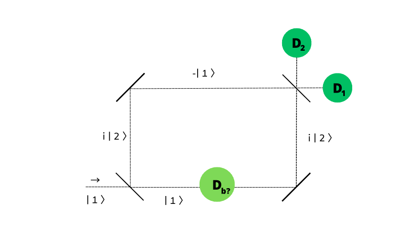
Figure 1: Elitsur-Vaidman bomb-tester experiment. The photon enters from the lower left corner to a Mach-Zehnder interferometry. The detection of the photon at the detector $D_{2}$ implies that the bomb is real, but that the photon has not interacted with the bomb.

3.3 Modified Stern-Gerlach set-up

The process (3.14) - the negative-result event - can also be regarded as a particular realization of the so-called repeatable experiment. A repeatable measurement is an exceptional class of experiments in which the microscopic system under study remains factorized (and intact) after the measurement, i.e., as

$$\left(\sum_{n}c_{n}|n\rangle\right)\otimes|\Phi_{0}\rangle\longrightarrow\sum_{n}c_{n}|n\rangle\otimes|\Phi_{n}\rangle\;,$$ (3.15)

or focusing on a single experiment with the result, $F=f_{m}$,

$$\left(\sum_{n}c_{n}|n\rangle\right)\to|m\rangle\;.$$ (3.16)

A simple example of the repeatable measurement is a variation of the Stern-Gerlach (SG) experiment. In the standard SG set-up (Fig. 2), an incoming beam of spin $\frac{1}{2}$ atom (e.g., $A_{g}$), travelling in the $\hat{x}$ direction, is sent into a region of inhomogeneous magnetic field, ${\bf B}=(0,0,f(z))$ with a strong gradient, $\partial f(z)/dz\neq 0$. The incident wave packet, is divided into two,

$$|\psi\rangle=c_{1}|\!\uparrow\rangle+c_{2}|\!\downarrow\rangle\;,\qquad|c_{1}|^{2}+|c_{2}|^{2}=1\;,$$ (3.17)

with the spin-up wave packet $|\!\!\uparrow\rangle$ is deflected upwards and the spin down component $|\!\!\downarrow\rangle$ downwards, as the atom proceeds towards $\hat{x}$ direction. On the screen they leave the two groups of blots whose intensities (the numbers of atoms) are proportional to $|c_{1}|^{2}:|c_{2}|^{2}$ after many atoms have been registered.

In a possible variation of the Stern-Gerlach set-up (Fig. 3), a detector $D$ is inserted in the region where the lower wave packet passes [21]. The screen behind the region of the inhomogeneous magnetic field is eliminated. $D$ is analogous to the set of detectors in the upper-hemisphere in Renninger’s set-up: it is a biased detector, capable of capturing and recording only the atoms in the spin-down state. For each single incident atom, $D$ either registers it (yes) or does not (no). In the first case, the spin has been measured to be in the state $s_{z}=-\tfrac{1}{2}$, but the atom itself gets lost in the complicated atom-detector interactions.

In the negative answer case (null measurement), no atom-detector interactions have taken place; nonetheless its spin state is determined to be $s_{z}=+\tfrac{1}{2}$. The atom is in the pure $|\!\!\uparrow\rangle$ state, and it can be used as the initial condition for subsequent analyses, for instance, with another SG set-ups with the magnets oriented in another direction, etc.

The whole discussion can be readily generalized to the case of atoms with spin $1$, $\tfrac{3}{2}$, etc. by appropriately enlarging the set of detectors, so as to extract and prepare the state of any chosen spin state $|s_{z}=m\rangle$, through interaction-free, null measurements.

The modified SG set-up we considered in this section can thus be seen as a simple, prototype version of Renninger’s negative-result experiment [21], as an example of the repeatable measurement, or as a typical “state preparation” process, illustrating well the fact that these three concepts are closely related to each other .

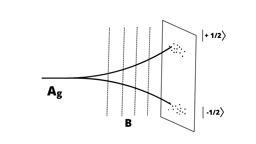
Figure 2: The standard SG set-up

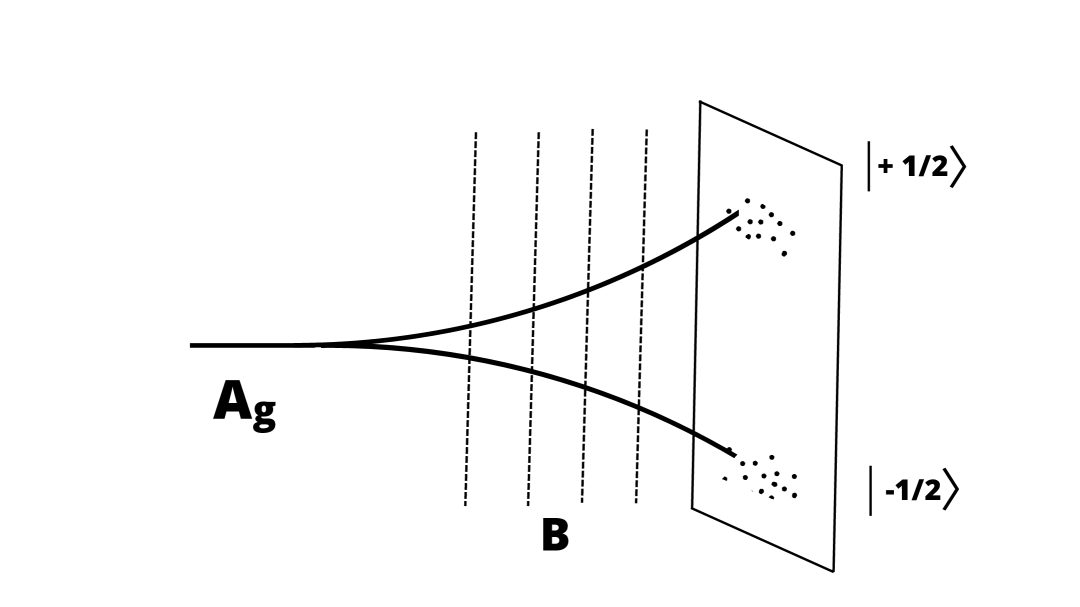
Figure 3: The modified SG set-up

4 Reflections

It is essential, in all negative-result experiments discussed in Sec. 3, that a very weak flux of the incident particles is used, such that processes with a single incident $\alpha$ particle, a photon, or an atom, are studied. Also, the experimental control must be good enough so that the expected time of arrival of each particle at the (biased) detector, is known with a reasonable precision. The reason is that, if it were not so, the non observation of certain event would not lead to any useful conclusion, as e.g., the particle may not yet have arrived, or has already passed, or is unknown when it will arrive, and so on.

In other words, an ideal null-measurement is a spacetime local event, albeit a virtual (i.e., missed) one . It represents the other side of the same medal of the standard quantum measurement processes each of which is a local spacetime event at its core [5]. This latter fact is the origin of the apparent “wave-function collapse”, as reviewed in Sec. 2.

Another important reflection is that the discussions of Sec. 3 illustrate nicely the well known fact about QM, i.e., that the wave-like behavior (the superposition, quantum nonlocality and interference) is the property of each single particle (the $\alpha$ particle, the photon and the atom discussed here, or the electron in Tonomura’s double-slit experiment [23]), and not due to a collective motion of, or correlation among, the particles in the beam.

The catchphrase “wave-particle duality” was used historically to describe the apparently schizophrenic behavior of the electrons, photons and atoms. In hindsight, though, this familiar expression left space for ambiguity and misunderstanding. For instance, it is an entirely different story that a large number of identical bosons form collective wavelike motions, such as the classical electromagnetic waves (light), or Bose-Einstein condensed cold atoms which are described in terms of a macroscopic wave function. So are all macroscopic quantum phenomena such as superconductivity and superfluidity, quantum Hall effects, and so on.

The wave-particle duality, a core idea of QM, is the property of each single quantum particle .

A last consideration: in this work we took it for granted that the $\alpha$ particle, the photon, and the silver atom, are all quantum particles. But what if a large molecule such as $C_{70}$ is used instead? Is it still a quantum particle? See [14, 24] for significant developments in our understanding of these questions.

The quest to grasp the very essential factors which can tell quantum-mechanical particles (the elementary particles, atomic nuclei, atoms, small molecules, etc.) from classical ones (the center of mass of isolated macroscopic bodies at finite body temperatures), leads us to the concept of Quantum Ratio [9].

References

- [1] E. Joos, H. D. Zeh, C. Kiefer, D. Giulini, J. Kupsch, I. O. Stamatescu, “Decoherence and the Appearance of a Classical World in Quantum Theory”, Springer, 2002.
- [2] J. A. Wheeler, W. H. Zurek, “Quantum Theory and Measurement”, Princeton NJ: Princeton University Press (1983).
- [3] J. S. Bell, “Speakable and unspeakable in quantum mechanics”, Cambridge University Press (1987).
- [4] A. Peres, “Quantum Theory: Concepts and Methods”, Dordrecht/Boston/London: Kluwer (1995).
- [5] K. Konishi, “Quantum fluctuations, particles and entanglement: a discussion towards the solution of the quantum measurement problems,” Int. Journ. Mod. Phys. A 37 (2022) 2250113 [arXiv:2111.14723 [quant-ph]].
- [6] K. Konishi, “Quantum fluctuations, particles and entanglement: solving the quantum measurement problems,” J. Phys. Conf. Ser. 2533, no.1, 012009 (2023) doi:10.1088/1742-6596/2533/1/012009 [arXiv:2302.08892 [quant-ph]].
- [7] M. Renninger, “Messungen ohne Störung des Meßobjekts”, Zeitschrift für Physik, 158 417 (1960).
- [8] A. C. Elitzur, L. Vaidman, ”Quantum mechanical interaction-free measurements”, Foundations of Physics. 23 (7): 987 (1993).
- [9] K. Konishi, “Newton’s equations from quantum mechanics for a macroscopic body in the vacuum”, Int. Journ. Mod. Phys. A 38 (2023) 2350080 [arXiv:2209.07318 [quant-ph]].
- [10] E. Joos and H. D. Zeh, “The emergence of classical properties through interaction with the environment”, Z. Phys. B 59, 223-243 (1985).
- [11] W. H. Zurek, “Decoherence and the Transition from Quantum to Classical”, Physics Today 44, 10, 36 (1991); https://doi.org/10.1063/1.881293.
- [12] M. Tegmark, “Apparent wave function collapse caused by scattering,” Found. Phys. Lett. 6, 571 (1993) doi:10.1007/BF00662807 [arXiv:gr-qc/9310032 [gr-qc]].
- [13] W. H. Zurek, “Decoherence, einselection, and the quantum origins of the classical,” Rev. Mod. Phys. 75, 715-775 (2003) doi:10.1103/RevModPhys.75.715 [arXiv:quant-ph/0105127 [quant-ph]].
- [14] L. Hackermüller, K. Hornberger, B. Brezger, A. Zeilinger, M. Arndt, “Decoherence of matter waves by thermal emission of radiation”, Nature, 427, (2004) 711. arXiv:quant-ph/0402146.
- [15] J. F. Clauser and S. Li, “Talbot-vonLau atom interferometry with cold slow potassium,” Phys. Rev. A 49, no.4, R2213-R2216 (1994) doi:10.1103/physreva.49.r2213.
- [16] K. Hansen and E. E. B. Campbell, “Thermal radiation from small particles”, Phys. Rev. E 58 (1998), 5477.
- [17] D. Frauchiger, R. Renner, “Quantum theory cannot consistently describe the use of itself”, Nature Communications Vol. 9, Article number: 3711 (2018).
- [18] A. Daneri, A. Loinger, and G. M. Prosperi, “Quantum theory of measurement and ergodic conditions”, Nuclear Physics, 33 (1962) 297.
- [19] L. Rosenfeld, “The Measuring Processes in Quantum Mechanics”, Supp. Prog. Theor. Phys., Commemoration Issue for the 30th Anniversary of the Meson Theory by Dr. H. Yukawa (1965), 222.
- [20] J. M. Jauch, E. P. Wigner, M. M. Yanase, “Some Comments Concerning Measurements in Quantum Mechanics”, Il Nuovo Cimento, Vol. XLVIII, B (1967) 144.
- [21] A. Loinger, “Comments on a recent paper concerning the quantum theory of measurement”, Nucl. Phys. A 108 (1968) 245.
- [22] N. F. Mott, “The wave mechanics of -decay tracks”, Proc. Roy. Soc. London A126 79 (1929).
- [23] A. Tonomura, J. Endo, T. Matsuda, T. Kawasaki and H. Ezawa, “Dimonstration of single-electron buildup of interference pattern”, American Journal of Physics 57, (1989) 117.
- [24] M. Arndt and K. Hornberger, “Testing the limits of quantum mechanical superpositions”, Nature Physics 10 271-277 (2014), [arXiv:1410.0270v1 [quant-ph]].